Modern Physics, 3rd Edition - Jimmy The Lecturer · MODERN PHYSICS Third edition Kenneth S. Krane...
37
MODERN PHYSICS Third edition Kenneth S. Krane DEPARTMENT OF PHYSICS OREGON STATE UNIVERSITY JOHN WILEY & SONS, INC
Transcript of Modern Physics, 3rd Edition - Jimmy The Lecturer · MODERN PHYSICS Third edition Kenneth S. Krane...
MODERNPHYSICS
Third edition
K e n n e t h S. K r a n eD E P A R T M E N T O F P H Y S I C S
O R E G O N S T A T E U N I V E R S I T Y
JOHN WILEY & SONS, INC

Chapter 5THE SCHRODINGER EQUATION
Quantum mechanics provides a mathematical framework in which the description of aprocess often includes different and possibly contradictory outcomes. A favorite illustrationof that situation is the case of Schrodinger’s cat. The cat is confined in a chamber with aradioactive atom, the decay of which will trigger the release of poison from a vial. Becausewe don’t know exactly when that decay will occur, until an observation of the condition ofthe cat is made the quantum-mechanical description of the cat must include both ‘‘cat alive’’and ‘‘cat dead’’ components.
134 Chapter 5 | The Schrodinger Equation
The future behavior of a particle in a classical (nonrelativistic, nonquantum)situation may be predicted with absolute certainty using Newton’s laws. If aparticle interacts with its environment through a known force �F (which mightbe associated with a potential energy U), we can do the mathematics necessaryto solve Newton’s second law, �F = d�p/dt (a second-order, linear differentialequation), and find the particle’s location �r(t) and velocity �v(t) at all future timest. The mathematics may be difficult, and in fact it may not be possible to solve theequations in closed form (in which case an approximate solution can be obtainedwith the help of a computer). Aside from any such mathematical difficulties, thephysics of the problem consists of writing down the original equation �F = d�p/dtand interpreting its solutions �r(t) and �v(t). For example, a satellite or planetmoving under the influence of a 1/r2 gravitational force can be shown, after theequations have been solved, to follow exactly an elliptical path.
In the case of nonrelativistic quantum physics, the basic equation to be solvedis a second-order differential equation known as the Schrodinger equation. LikeNewton’s laws, the Schrodinger equation is written for a particle interacting withits environment, although we describe the interaction in terms of the potentialenergy rather than the force. Unlike Newton’s laws, the Schrodinger equationdoes not give the trajectory of the particle; instead, its solution gives the wavefunction of the particle, which carries information about the particle’s wavelikebehavior. In this chapter we introduce the Schrodinger equation, obtain some of itssolutions for certain potential energies, and learn how to interpret those solutions.
5.1 BEHAVIOR OF A WAVE AT A BOUNDARY
In studying wave motion, we often must analyze what occurs when a wavemoves from one region or medium to a different region or medium in which theproperties of the wave may change. For example, when a light wave moves fromair into glass, its wavelength and the amplitude of its electric field both decrease.At every such boundary, a portion of the incident wave intensity is transmittedinto the second medium and a portion is reflected back into the first medium.
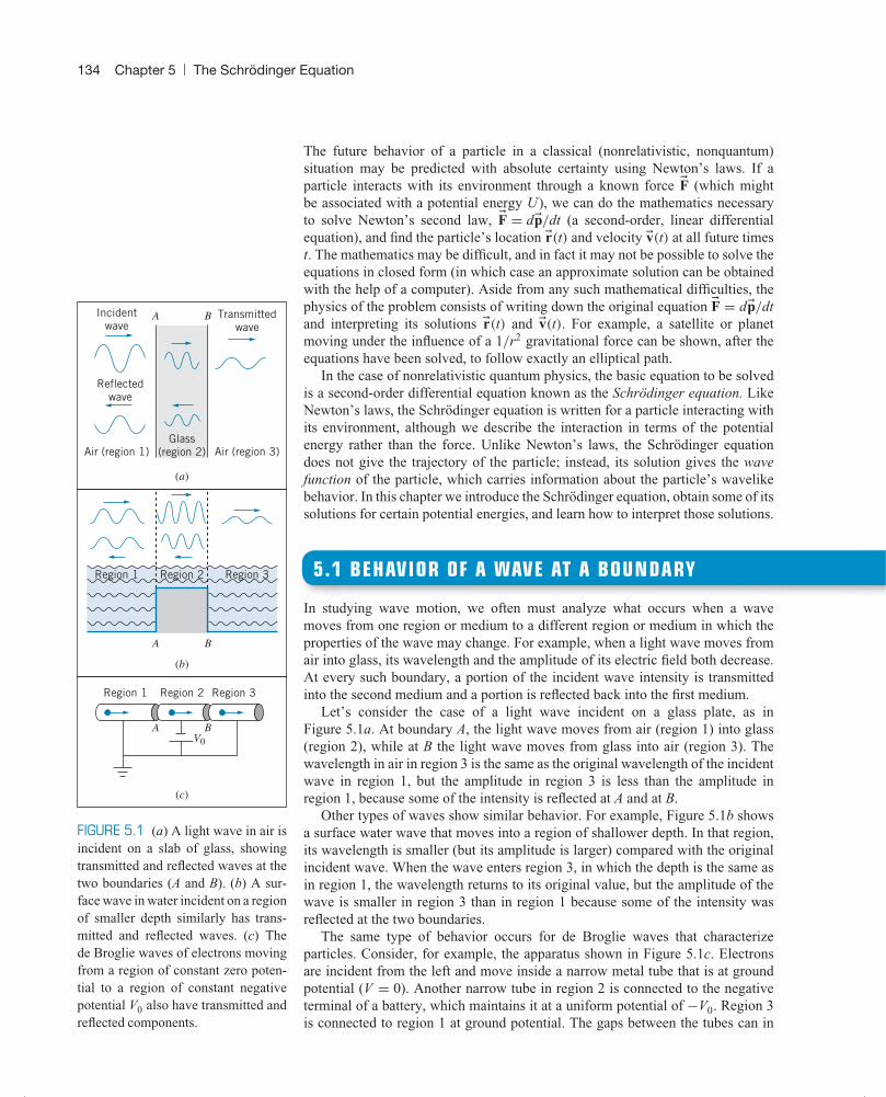
Let’s consider the case of a light wave incident on a glass plate, as inFigure 5.1a. At boundary A, the light wave moves from air (region 1) into glass(region 2), while at B the light wave moves from glass into air (region 3). Thewavelength in air in region 3 is the same as the original wavelength of the incidentwave in region 1, but the amplitude in region 3 is less than the amplitude inregion 1, because some of the intensity is reflected at A and at B.
(a)
(b)
(c)
Incidentwave
Reflectedwave
Air (region 1) Air (region 3)
Region 3Region 2Region 1
Region 3
V0
Region 2Region 1
Transmittedwave
Glass(region 2)
A B
A B
A B
FIGURE 5.1 (a) A light wave in air isincident on a slab of glass, showingtransmitted and reflected waves at thetwo boundaries (A and B). (b) A sur-face wave in water incident on a regionof smaller depth similarly has trans-mitted and reflected waves. (c) Thede Broglie waves of electrons movingfrom a region of constant zero poten-tial to a region of constant negativepotential V0 also have transmitted andreflected components.
Other types of waves show similar behavior. For example, Figure 5.1b showsa surface water wave that moves into a region of shallower depth. In that region,its wavelength is smaller (but its amplitude is larger) compared with the originalincident wave. When the wave enters region 3, in which the depth is the same asin region 1, the wavelength returns to its original value, but the amplitude of thewave is smaller in region 3 than in region 1 because some of the intensity wasreflected at the two boundaries.
The same type of behavior occurs for de Broglie waves that characterizeparticles. Consider, for example, the apparatus shown in Figure 5.1c. Electronsare incident from the left and move inside a narrow metal tube that is at groundpotential (V = 0). Another narrow tube in region 2 is connected to the negativeterminal of a battery, which maintains it at a uniform potential of −V0. Region 3is connected to region 1 at ground potential. The gaps between the tubes can in

5.1 | Behavior of a Wave at a Boundary 135
principle be made so small that we can regard the changes in potential at A and B asoccurring suddenly. In region 1, the electrons have kinetic energy K, momentump = √
2mK, and de Broglie wavelength λ = h/p. In region 2, the potential energyfor the electrons is U = qV = (−e)(−V0) = +eV0. We assume that the originalkinetic energy of the electrons in region 1 is greater than eV0, so that the electronsmove into region 2 with a smaller kinetic energy (equal to K − eV0), a smallermomentum, and thus a greater wavelength. When the electrons move from region2 into region 3, they gain back the lost kinetic energy and move with their originalkinetic energy K and thus with their original wavelength. As in the case of thelight wave or the water wave, the amplitude of the de Broglie wave in region 3is smaller than in region 1, meaning that the current of electrons in region 3 issmaller than the incident current, because some of the electrons are reflected atthe boundaries at A and B.
We can thus identify a total of 5 waves moving in the three regions: (1) a wavemoving to the right in region 1 (the incident wave); (2) a wave moving to the leftin region 1 (representing the net combination of waves reflected from boundary Aplus waves reflected from boundary B and then transmitted through boundary Aback into region 1); (3) a wave moving to the right in region 2 (representing wavestransmitted through boundary A plus waves reflected at B and then reflected againat A); (4) a wave moving to the left in region 2 (waves reflected at B); and (5)a wave moving to the right in region 3 (the transmitted waves at boundary B).Because we are assuming that waves are incident from region 1, it is not possibleto have a wave moving to the left in region 3.
Penetration of the Reflected WaveAnother property of classical waves that carries over into quantum waves ispenetration of a totally reflected wave into a forbidden region. When a lightwave is completely reflected from a boundary, an exponentially decreasing wavecalled the evanescent wave penetrates into the second medium. Because 100%of the light wave intensity is reflected, the evanescent wave carries no energyand so cannot be directly observed in the second medium. But if we make thesecond medium very thin (perhaps equal to a few wavelengths of light) the lightwave can emerge on the opposite side of the second medium. We’ll discuss thisphenomenon in more detail at the end of this chapter.
The same effect occurs with de Broglie waves. Suppose we increase the batteryvoltage in Figure 5.1c so that the potential energy in region 2 (equal to eV0)is greater than the initial kinetic energy in region 1. The electrons do not haveenough energy to enter region 2 (they would have negative kinetic there) and soall electrons are reflected back into region 1.
Like light waves, de Broglie waves can also penetrate into the forbidden regionwith exponentially decreasing amplitudes. However, because de Broglie wavesare associated with the motion of electrons, that means that electrons must alsopenetrate a short distance into the forbidden region. The electrons cannot bedirectly observed in that region, because they have negative kinetic energy there.Nor can we do any experiment that would reveal their “real” existence in theforbidden region, such as measuring the speed of their passage through that regionor detecting the magnetic field that their motion might produce.
One explanation for the penetration of the electrons into the forbidden regionrelies on the uncertainty principle—because we can’t know exactly the energy ofthe incident electrons, we can’t say with certainty that they don’t have enoughkinetic energy to penetrate into the forbidden region. For short enough time �t, the

136 Chapter 5 | The Schrodinger Equation
energy uncertainty �E ∼ −h/�t might allow the electron to travel a short distanceinto the forbidden region, but this extra energy does not “belong to” the electronin any permanent sense. Later in this chapter we’ll discuss a more mathematicalapproach to this explanation of penetration into the forbidden region.
Continuity at the Boundaries
When a wave such as a light wave or a water wave crosses a boundary as inFigure 5.1, the mathematical function that describes the wave must have twoproperties at each boundary:
1. The wave function must be continuous.2. The slope of the wave function must be continuous, except when the boundary
height is infinite.
Figure 5.2a shows a discontinuous wave function; the wave displacementchanges suddenly at a single location. This type of behavior is not allowed.Figure 5.2b shows a continuous wave function (there are no gaps) with adiscontinuous slope. This type of behavior is also not allowed, unless theboundary is of infinite height. Figures 5.2c, d show how two sine curves and anexponential and a sine can be joined so that both the function and the slope arecontinuous.
(b)
(a)
(c)
(d)
FIGURE 5.2 (a) A discontinuouswave. (b) A continuous wave witha discontinuous slope. (c) Two sinewaves join smoothly. (d) A sine waveand an exponential join smoothly.
Across any non-infinite boundary, the wave must be smooth—no gaps in thefunction and no sharp changes in slope. When we solve for the mathematicalform of a wave function, there are usually undetermined parameters, such asthe amplitude and phase of the wave. In order to make the wave smooth atthe boundary, we obtain the values of those coefficients by applying the twoboundary conditions to make the function and its slope continuous. For example,at boundary A in Figure 5.1, we first evaluate the total wave function in region 1at A and set it equal to the wave function in region 2 at A. This guarantees that thetotal wave function is continuous at A. We then take the derivative of the wavefunction in region 1, evaluate it at A, and set that equal to the derivative of thewave function in region 2 evaluated at A. This step makes the slope in region 1match the slope in region 2 at boundary A. These two steps give us two equationsrelating the parameters of the waves and allow us to find relationships betweenthe amplitudes and phases of the waves in regions 1 and 2. The process mustbe repeated at every boundary, such as at B in Figure 5.1 to match the waves inregions 2 and 3.
We can understand the exception to the continuity of the slope for infiniteboundaries with an example from classical physics. Imagine a ball dropped froma height y = H above a stretched rubber sheet at y = 0. The ball falls freelyunder gravity until it strikes the sheet, which we assume behaves like an elasticspring. The sheet stretches as the ball is brought to rest, after which the restoringforce propels the ball upward. The motion of the ball might be represented byFigure 5.3. Above the sheet (y > 0) the motion is represented by parabolas, andwhile the ball is in contact with the sheet (y < 0) the motion is described by sinecurves. Note how the curves join smoothly at y = 0, and note how both y(t) andits derivative v(t) are continuous.
Sine
Parabola
t
y(t)
v(t)
H
0
0t
FIGURE 5.3 The position and veloc-ity of a ball dropped from a heightH above a springlike rubber sheet aty = 0.
On the other hand, imagine a ball hitting a steel surface, which we assume to beperfectly rigid. The ball rebounds elastically, and at the instant it is in contact withthe surface its velocity reverses direction. The motion of the ball is represented
5.1 | Behavior of a Wave at a Boundary 137
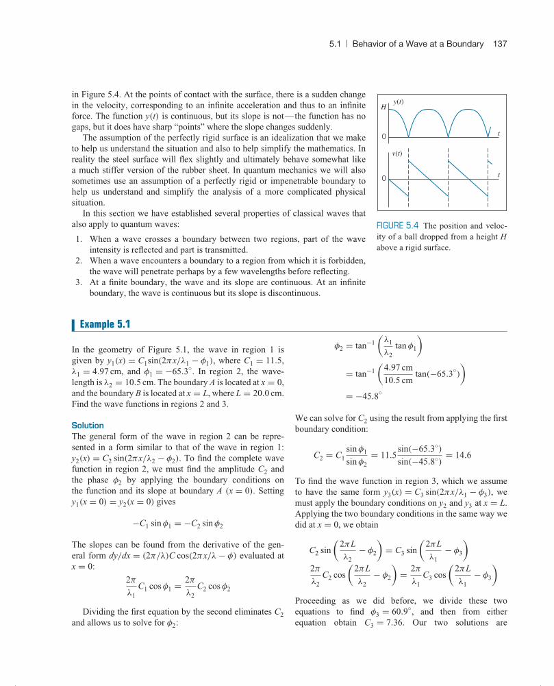
in Figure 5.4. At the points of contact with the surface, there is a sudden changein the velocity, corresponding to an infinite acceleration and thus to an infiniteforce. The function y(t) is continuous, but its slope is not—the function has nogaps, but it does have sharp “points” where the slope changes suddenly.
The assumption of the perfectly rigid surface is an idealization that we maketo help us understand the situation and also to help simplify the mathematics. Inreality the steel surface will flex slightly and ultimately behave somewhat likea much stiffer version of the rubber sheet. In quantum mechanics we will alsosometimes use an assumption of a perfectly rigid or impenetrable boundary tohelp us understand and simplify the analysis of a more complicated physicalsituation.
t
y(t)
v(t)
H
0
0 t
FIGURE 5.4 The position and veloc-ity of a ball dropped from a height Habove a rigid surface.
In this section we have established several properties of classical waves thatalso apply to quantum waves:
1. When a wave crosses a boundary between two regions, part of the waveintensity is reflected and part is transmitted.
2. When a wave encounters a boundary to a region from which it is forbidden,the wave will penetrate perhaps by a few wavelengths before reflecting.
3. At a finite boundary, the wave and its slope are continuous. At an infiniteboundary, the wave is continuous but its slope is discontinuous.
Example 5.1
In the geometry of Figure 5.1, the wave in region 1 isgiven by y1(x) = C1sin(2πx/λ1 − φ1), where C1 = 11.5,λ1 = 4.97 cm, and φ1 = −65.3◦. In region 2, the wave-length is λ2 = 10.5 cm. The boundary A is located at x = 0,and the boundary B is located at x = L, where L = 20.0 cm.Find the wave functions in regions 2 and 3.
SolutionThe general form of the wave in region 2 can be repre-sented in a form similar to that of the wave in region 1:y2(x) = C2 sin(2πx/λ2 − φ2). To find the complete wavefunction in region 2, we must find the amplitude C2 andthe phase φ2 by applying the boundary conditions onthe function and its slope at boundary A (x = 0). Settingy1(x = 0) = y2(x = 0) gives
−C1 sin φ1 = −C2 sin φ2
The slopes can be found from the derivative of the gen-eral form dy/dx = (2π/λ)C cos(2πx/λ − φ) evaluated atx = 0:
2π
λ1C1 cos φ1 = 2π
λ2C2 cos φ2
Dividing the first equation by the second eliminates C2and allows us to solve for φ2:
φ2 = tan−1
(λ1
λ2tan φ1
)
= tan−1
(4.97 cm
10.5 cmtan(−65.3◦
)
)
= −45.8◦
We can solve for C2 using the result from applying the firstboundary condition:
C2 = C1sin φ1
sin φ2= 11.5
sin(−65.3◦)
sin(−45.8◦)= 14.6
To find the wave function in region 3, which we assumeto have the same form y3(x) = C3 sin(2πx/λ1 − φ3), wemust apply the boundary conditions on y2 and y3 at x = L.Applying the two boundary conditions in the same way wedid at x = 0, we obtain
C2 sin
(2πL
λ2− φ2
)= C3 sin
(2πL
λ1− φ3
)2π
λ2C2 cos
(2πL
λ2− φ2
)= 2π
λ1C3 cos
(2πL
λ1− φ3
)
Proceeding as we did before, we divide these twoequations to find φ3 = 60.9◦, and then from eitherequation obtain C3 = 7.36. Our two solutions are

138 Chapter 5 | The Schrodinger Equation
then y2(x) = 14.6 sin (2πx/10.5 + 45.8◦) and y3(x) =
7.36 sin(2πx/4.97 + 14.6◦), with x measured in cm.
Figure 5.5 shows the wave in all three regions. Notehow the waves join smoothly at the boundaries.
How is it possible that the amplitude of y2 can be greaterthan the amplitude of y1? Keep in mind that y1 representsthe total wave in region 1, which includes the incident waveand the reflected wave. Depending on the phase differencebetween them, when the incident and reflected waves areadded to obtain y1, the amplitude of the resultant can besmaller than the amplitude of either wave.
10
10
−10
−10 20 30
FIGURE 5.5 Example 5.1.
5.2 CONFINING A PARTICLE
A free particle (that is, a particle on which no forces act anywhere) is by definitionnot confined, so it can be located anywhere. It has, as we discussed in Chapter 4,a definite wavelength, momentum, and energy (for which we can choose anyvalue).
A confined particle, on the other hand, is represented by a wave packet thatmakes it likely to be found only in a region of space of size �x. We constructsuch a wave packet by adding together different sine or cosine waves to obtainthe desired mathematical shape.
In quantum mechanics, we often want to analyze the behavior of confinedparticles, for example an electron that is attached to a specific atom or molecule.We’ll consider the properties of atomic electrons beginning in Chapter 6, but fornow let’s look at a simpler problem: an electron moving in one dimension andconfined by a series of electric fields. Figure 5.6 shows how the apparatus ofFigure 5.1c might be modified for this purpose. The center section is grounded(so that V = 0) and the two side sections are connected to batteries so that theyare at potentials of −V0 relative to the center section. As before, we assume thatthe gaps between the center section and the side sections can be made as narrowas possible, so we can regard the potential energy as changing instantaneously atthe boundaries A and B. This arrangement is often called a potential energy well.
(a)
(b)
U = U0
U = 0
V0V0
A B
L
FIGURE 5.6 (a) Apparatus for con-fining an electron to the center regionof length L. (b) The potential energyof an electron in this apparatus.
The potential energy of an electron in this situation is then 0 in the centersection and U0 = qV = (−e)(−V0) = +eV0 in the two side sections as shown inFigure 5.6. To confine the electron, we want to consider cases in which it movesin the center section with a kinetic energy K that is less than U0. For example, theelectron might have a kinetic energy of 5 eV in the center section, and the sidesections might have potential energies of 10 eV. The electron thus does not haveenough energy to “climb” the potential energy hill between the center section andthe side sections, and (at least from the classical point of view) the electron isconfined to the center section.
We’ll discuss the full solution to this problem later in this chapter, but for nowlet’s simplify even further and consider the case of an infinitely high potentialenergy barrier at A and B. This is a good approximation to the situation inwhich the kinetic energy of the electron in the center section is much smallerthan the potential energy supplied by the batteries. In this case the penetration

5.2 | Confining a Particle 139
into the forbidden region, which we discussed in Section 5.1, cannot occur. Theprobability to find the electron in either of the side regions is therefore preciselyzero everywhere in those regions, and thus the wave amplitude is zero everywherein those regions, including at the boundaries (locations A and B). For the wavefunction to be continuous, the wave function in the center section must havevalues of zero at A and B.
Of all the possible waves that might be used to describe the particle in thiscenter section, the continuity condition restricts us to waves that have zeroamplitude at the boundaries. Some of those waves are illustrated in Figure 5.7.Note that the wave function is continuous, but its slope is not (there are sharppoints in the function at locations A and B). This is an example of the exceptionto the second boundary condition—the slope may be discontinuous at an infinitebarrier.
L = ½λ
L = λ3 2
L = 2λ
L = λ
A B
A B
A B
A B
FIGURE 5.7 Some possible wavesthat might be used to describe an elec-tron confined by an infinite potentialenergy barrier to a region of length L.
In contrast to the free particle for which the wavelength could have any value,only certain values of the wavelength are allowed. The de Broglie relationship thentells us that only certain values of the momentum are allowed, and consequentlyonly certain values of the energy are allowed. The energy is not a continuousvariable, free to take on any arbitrary value; instead, the energy is a discretevariable that is restricted to a certain set of values. This is known as quantizationof energy.
You can see directly from Figure 5.7 that the allowed wavelengths are2L, L, 2L/3, . . ., where L is the length of the center section. We can write thesewavelengths as
λn = 2L
nn = 1, 2, 3, . . . (5.1)
This set of wavelengths is identical to the wavelengths of the classical problemof standing waves on a string stretched between two points. From the de Broglierelationship λ = h/p we obtain
pn = nh
2L(5.2)
The energy of the particle in the center section is only kinetic energy p2/2m,and so
En = n2 h2
8mL2(5.3)
These are the allowed or quantized values of the energy of the electron.A wave packet describing the electron in this region must be a combination of
waves with the allowed values of the wavelengths. However, it is not necessaryto construct a wave packet from a combination of waves to describe this confinedparticle. Even a single one of these waves represents the confined particle, becausethe wave function must be zero in the forbidden regions. So the waveforms shownin Figure 5.7 can represent wave packets of this confined electron, each wavepacket consisting of only a single wave.
The appearance of energy quantization accompanies every attempt to confinea particle to a finite region of space. Quantization of energy is one of the principalfeatures of the quantum theory, and studying the quantized energy levels ofsystems (such as by observing the energies of emitted photons) is an importanttechnique of experimental physics that gives us information about the propertiesof atoms and nuclei.

140 Chapter 5 | The Schrodinger Equation
Applying the Uncertainty Principleto a Confined ParticleIn Chapter 4 we constructed wave packets and showed how the uncertaintyprinciple related the size of the wave packet to the range of wavelengths thatwas used in its construction. Let’s now see how the Heisenberg uncertaintyrelationships apply in the case of a confined particle.
In the arrangement of Figure 5.6 (with infinitely high barriers on each side),the particle is known to be somewhere in the center section of the apparatus, andthus �x ∼ L is a reasonable estimate of the uncertainty in its location. To find theuncertainty in its momentum, we use the rigorous definition of uncertainty givenin Eq. 4.15: �px = √
(p2x)av − (px,av)
2 . The particle moving in the center sectioncan be considered to be moving to the left or to the right with equal probability(just as the classical standing-wave problem can be analyzed as the superpositionof identical waves moving to the left and to the right). Thus px,av = 0. If theparticle is moving with a momentum given by Eq. 5.2, p2
x = (nh/L)2 and so�px = nh/L. Combining the uncertainties in position and momentum, we have
�x�px ∼ Lnh
L= nh (5.4)
The product of the uncertainties is certainly greater than −h/2, and so the resultof confining the particle is entirely consistent with the Heisenberg uncertaintyrelationship. Note that even the smallest possible value of the product of theuncertainties (which is obtained for n = 1) is still much larger than the minimumvalue given by the uncertainty principle.
Later in this chapter, we will use a more rigorous way to evaluate the uncertaintyin position using a formula similar to Eq. 4.15 to find the uncertainty in position,and we will find that the result does not differ very much from the estimateof Eq. 5.4.
5.3 THE SCHRODINGER EQUATION
The differential equation whose solution gives us the wave behavior of particles iscalled the Schrodinger equation. It was developed in 1926 by Austrian physicistErwin Schrodinger. The equation cannot be derived from any previous lawsor postulates; like Newton’s equations of motion or Maxwell’s equations ofelectromagnetism, it is a new and independent result whose correctness canbe determined only by comparing its predictions with experimental results.For nonrelativistic motion, the Schrodinger equation gives results that correctlyaccount for observations at the atomic and subatomic level.
Erwin Schrodinger (1887–1961, Aus-tria). Although he disagreed with theprobabilistic interpretation that waslater given to his work, he devel-oped the mathematical theory of wavemechanics that for the first time per-mitted the wave behavior of physicalsystems to be calculated.
We can justify the form of the Schrodinger equation by examining the solutionexpected for the free particle, which should give a wave whose shape at anyparticular time, specified by the wave function ψ(x), is that of a simple deBroglie wave, such as ψ(x) = A sin kx, where A is the amplitude of the wave andk = 2π/λ. If we are looking for a differential equation, then we need to take somederivatives:
dψ
dx= kA cos kx,
d2ψ
dx2= −k2A sin kx = −k2ψ(x)

5.3 | The Schrodinger Equation 141
Note that the second derivative gives the original function again. With the kineticenergy K = p2/2m = (h/λ)2/2m = −h2k2/2m, we can then write
d2ψ
dx2= −k2ψ(x) = −2m
−h2Kψ(x) = −2m
−h2(E − U)ψ(x)
where E = K + U is the nonrelativistic total energy of the particle. For a freeparticle, U = 0 so E = K; however, we are using the free particle solution to tryto extend to the more general case in which there is a potential energy U(x). Theequation then becomes
−−h2
2m
d2ψ
dx2+ U(x)ψ(x) = Eψ(x) (5.5)
Equation 5.5 is the time-independent Schrodinger equation for one-dimensionalmotion.
The solution to Eq. 5.5 gives the shape of the wave at time t = 0. Themathematical function that describes a one-dimensional traveling wave mustinvolve both x and t. This wave is represented by the function (x,t):
(x,t) = ψ(x)e−iωt (5.6)
The time dependence is given by the complex exponential function e−iωt withω = E/−h. (You can find a few useful formulas involving complex numbers inAppendix B.) We’ll discuss the time-dependent part later in this chapter. For now,we’ll concentrate on the time-independent function ψ(x).
We assume that we know the potential energy U(x), and we wish to obtain thewave function ψ(x) and the energy E for that potential energy. This is a generalexample of a type of problem known as an eigenvalue problem; we find that it ispossible to obtain solutions to the equation only for particular values of E, whichare known as the energy eigenvalues.
The general procedure for solving the Schrodinger equation is as follows:
1. Begin by writing Eq. 5.5 with the appropriate U(x). Note that if the potentialenergy changes discontinuously [U(x) may be represented by a discontinuousfunction; ψ(x) may not], we may need to write different equations for differentregions of space. Examples of this sort are given in Section 5.4.
2. Using general mathematical techniques suited to the form of the equation, finda mathematical function ψ(x) that is a solution to the differential equation.Because there is no one specific technique for solving differential equations,we will study several examples to learn how to find solutions.
3. In general, several solutions may be found. By applying boundary conditionssome of these may be eliminated and some arbitrary constants may bedetermined. It is generally the application of the boundary conditions thatselects out the allowed energies.
4. If you are seeking solutions for a potential energy that changes discontinuously,you must apply the continuity conditions on ψ(x) (and usually on dψ/dx) atthe boundary between different regions.
Because the Schrodinger equation is linear, any constant multiplying a solutionis also a solution. The method to determine the amplitude of the wave function isdiscussed in the next section.

142 Chapter 5 | The Schrodinger Equation
|ψ (x)|2
dx
x1 x2
FIGURE 5.8 The probability to findthe particle in a small region of widthdx is equal to the area of the strip underthe |ψ(x)|2 curve. The total probabilityto find the particle between x1 and x2 isthe sum of the areas of the strips, equalto the integral between those limits.
Probabilities and NormalizationThe remaining steps in the procedure for applying the Schrodinger recipe dependon the physical interpretation of the solution to the differential equation. Ouroriginal goal in solving the Schrodinger equation was to obtain the wave propertiesof the particle. What does the amplitude of ψ(x) represent, and what is the physicalvariable that is waving? It is certainly not a displacement, as in the case of a waterwave or a wave on a stretched piano wire, nor is it a pressure wave, as in the caseof sound. It is a very different kind of wave, whose squared absolute amplitudegives the probability for finding the particle in a given region of space.
If we define P(x) as the probability density (probability per unit length, in onedimension), then according to the Schrodinger recipe
P(x) dx = |ψ(x)|2 dx (5.7)
as indicated in Figure 5.8. In Eq. 5.7, |ψ(x)|2 dx gives the probability to find theparticle in the interval dx at x (that is, between x and x + dx).∗ Because the wavefunction ψ(x) might be a complex function, it is necessary to square its absolutemagnitude to make sure that the probability is a positive real number.
The squared magnitude of the general time-dependent wave function(Eq. 5.6) is:
| (x,t)|2 = |ψ(x)|2|e−iωt|2 = |ψ(x)|2 (5.8)
where the last step can be taken because the magnitude of the time-dependentfactor is 1. For this reason, the probability density associated with a solution tothe Schrodinger equation (for any allowed value of E) is independent of time.These special quantum states are called stationary states.
This interpretation of |ψ(x)|2 helps us to understand the continuity conditionof ψ(x). We must not allow the probability to change discontinuously, but, likeany well-behaved wave, the probability to locate the particle varies smoothly andcontinuously.
This interpretation of ψ(x) now permits us to complete the Schrodinger recipeand to illustrate how to use the wave function to calculate quantities that we canmeasure in the laboratory. Steps 1 through 4 were given previously; the recipecontinues:
5. For a wave function describing a single particle, the probability summed overall locations must give 100%—that is, the particle must be located somewherebetween x = −∞ and x = +∞. The probability to find the particle in a smallinterval was given in Eq. 5.7. The total probability to find the particle in allsuch intervals must be exactly 1:∫ +∞
−∞|ψ(x)|2 dx = 1 (5.9)
The Schrodinger equation is linear, which means that if ψ(x) is a solutionthen any constant times ψ(x) is also a solution. For the probability to be ameaningful concept, this constant must be chosen so that Eq. 5.9 is satisfied.
∗It is not correct to speak of “the probability to find the particle at the point x.” A single point is amathematical abstraction with no physical dimension. The probability of finding a particle at a pointis zero, but there can be a nonzero probability of finding the particle in an interval.

5.3 | The Schrodinger Equation 143
A wave function with its multiplicative constant chosen in this way is said tobe normalized, and Eq. 5.9 is known as the normalization condition.
6. Because the solution to the Schrodinger equation represents a probability,any solution that becomes infinite must be discarded—it makes no senseto have an infinite probability to find a particle in any interval. In practice,we “discard” a solution by setting its multiplicative constant equal to zero.For example, if the mathematical solution to the differential equation yieldsψ(x) = Aekx + Be−kx for the entire region x > 0, then we must require A = 0for the solution to be physically meaningful; otherwise |ψ(x)|2 would becomeinfinite as x goes to infinity. On the other hand, if this solution is to be validin the entire region x < 0, then we must set B = 0. However, if the solution isto be valid only in a small portion of the range of x—say, 0 < x < L—thenwe cannot set either A = 0 or B = 0.
7. Suppose the interval between two points x1 and x2 is divided into a series ofinfinitesimal intervals of width dx (Figure 5.8). To find the total probability forthe particle to be located between x1 and x2, which we represent as P(x1: x2),we calculate the sum of all the probabilities P(x) dx in each interval dx. Thissum can be expressed as an integral:
P(x1: x2) =∫ x2
x1
P(x) dx =∫ x2
x1
|ψ(x)|2 dx (5.10)
If the wave function has been properly normalized, Eq. 5.10 will always yielda probability that lies between 0 and 1.
8. Because we can no longer speak with certainty about the position of theparticle, we can no longer guarantee the outcome of a single measurement ofany physical quantity that depends on its position. Instead, we can find theaverage outcome of a large number of measurements. For example, supposewe wish to find the average location of a particle by measuring its coordinatex. From a large number of measurements, we find the value x1 a certainnumber of times n1, x2 a number of times n2, etc., and in the usual way wecan find the average value
xav = n1x1 + n2x2 + · · ·n1 + n2 + · · · =
∑nixi∑ni
(5.11)
The number of times ni that we measure each xi is proportional to theprobability P(xi)dx to find the particle in the interval dx at xi. Making thissubstitution and changing the sums to integrals, we have
xav =
∫ +∞
−∞P(x)x dx∫ +∞
−∞P(x) dx
=∫ +∞
−∞|ψ(x)|2x dx (5.12)
where the last step can be made if the wave function is normalized, in whichcase the denominator of Eq. 5.12 is equal to one.
By analogy, the average value of any function of x can be found:
[f (x)]av =∫ +∞
−∞P(x)f (x) dx =
∫ +∞
−∞|ψ(x)|2f (x) dx (5.13)
Average values calculated according to Eq. 5.12 or 5.13 are known asexpectation values.

144 Chapter 5 | The Schrodinger Equation
5.4 APPLICATIONS OF THE SCHRODINGEREQUATION
Solutions for Constant Potential EnergyFirst let’s examine the solutions to the Schrodinger equation for the special caseof a constant potential energy, equal to U0. Then Eq. 5.5 becomes
−−h2
2m
d2ψ
dx2+ U0ψ(x) = Eψ(x) (5.14)
or (assuming for now that E > U0)
d2ψ
dx2= −k2ψ(x) with k =
√2m(E − U0)
−h2(5.15)
The parameter k in this equation is equal to the wave number 2π/λ.The solution to Eq. 5.15 is a function of x that, when differentiated twice, gives
back the original function multiplied by the negative constant −k2. The functionthat has this property is sin kx or cos kx. The most general solution to the equation is
ψ(x) = A sin kx + B cos kx (5.16)
The constants A and B must be determined by applying the continuity andnormalization requirements. We can demonstrate that Eq. 5.16 satisfies Eq. 5.15by taking two derivatives:
dψ
dx= kA cos kx − kB sin kx
d2ψ
dx2= −k2A sin kx − k2B cos kx = −k2(A sin kx + B cos kx) = −k2ψ(x)
so the original equation is indeed satisfied.To analyze the penetration of a particle into a forbidden region, we must
consider the case in which the energy E of the particle is smaller than the potentialenergy U0. For this case we can rewrite Eq. 5.14 as
d2ψ
dx2= k′2ψ(x) with k′ =
√2m(U0 − E)
−h2(5.17)
In this case the general solution in the forbidden regions is
ψ(x) = Aek′x + Be−k′x (5.18)
Once again, we can demonstrate that Eq. 5.18 is a solution of Eq. 5.17 by takingtwo derivatives:
dψ
dx= k′Aek′x − k′Be−k′x
d2ψ
dx2= k′2Aek′x + k′2Be−k′x = k′2(Aek′x + Be−k′x) = k′2ψ(x)
We will use Eqs. 5.16 and 5.18 as our solutions to the Schrodinger equation forconstant potential energy in the allowed (E > U0) and forbidden (E < U0) regions.

5.4 | Applications of the Schrodinger Equation 145
The Free ParticleFor a free particle, the force is zero and so the potential energy is constant. Wemay choose any value for that constant, so for convenience we’ll choose U0 = 0.The solution is given by Eq. 5.16, ψ(x) = A sin kx + B cos kx. The energy of theparticle is
E =−h2k2
2m(5.19)
Our solution has placed no restrictions on k, so the energy is permitted to haveany value (in the language of quantum physics, we say that the energy is not quan-tized). We note that Eq. 5.19 is the kinetic energy of a particle with momentump = −hk or, equivalently, p = h/λ. This is as we would have expected, becausethe free particle can be represented by a de Broglie wave with any wavelength.
Solving for A and B presents some difficulties because the normalizationintegral, Eq. 5.9, cannot be evaluated from −∞ to +∞ for this wave function.We therefore cannot determine probabilities for the free particle from the wavefunction of Eq. 5.16.
It is also instructive to write the wave function in terms of complex exponentials,using sin kx = (eikx − e−ikx)/2i and cos kx = (eikx + e−ikx)/2:
ψ(x) = A
(eikx − e−ikx
2i
)+ B
(eikx + e−ikx
2
)= A′eikx + B′e−ikx (5.20)
where A′ = A/2i + B/2 and B′ = −A/2i + B/2. To interpret this solution in termsof waves we form the complete time-dependent wave function using Eq. 5.6:
(x,t) = (A′eikx + B′e−ikx)e−iωt = A′ei(kx−ωt) + B′e−i(kx+ωt) (5.21)
The dependence of the first term on kx − ωt identifies this term as representinga wave moving to the right (in the positive x direction) with amplitude A′, andthe second term involving kx + ωt represents a wave moving to the left (in thenegative x direction) with amplitude B′.
If we want the wave to represent a beam of particles moving in the +x direction,then we must set B′ = 0. The probability density associated with this wave isthen, according to Eq. 5.7,
P(x) = |ψ(x)|2 = |A′|2eikxe−ikx = |A′|2 (5.22)
The probability density is constant, meaning the particles are equally likely to befound anywhere along the x axis. This is consistent with our discussion of the free-particle de Broglie wave in Chapter 4—a wave of precisely defined wavelengthextends from x = −∞ to x = +∞ and thus gives a completely unlocalizedparticle.
Infinite Potential Energy WellNow we’ll consider the formal solution to the problem we discussed in Section 5.2:a particle is trapped in the region between x = 0 and x = L by infinitely highpotential energy barriers. Imagine an apparatus like that of Figure 5.6, in which theparticle moves freely in this region and makes elastic collisions with the perfectlyrigid barriers that confine it. This problem is sometimes called “a particle in abox.” For now we’ll assume that the particle moves in only one dimension; laterwe’ll expand to two and three dimensions.

146 Chapter 5 | The Schrodinger Equation
The potential energy may be expressed as:
U(x) = 0 0 ≤ x ≤ L
= ∞ x < 0, x > L (5.23)
The potential energy is shown in Figure 5.9. We are free to choose any constantvalue for U in the region 0 ≤ x ≤ L; we choose it to be zero for convenience.
U = ∞
To ∞ To ∞
U = ∞U = 0
x = 0 x = L
FIGURE 5.9 The potential energy of aparticle that moves freely (U = 0) inthe region 0 ≤ x ≤ L but is completelyexcluded (U = ∞) from the regionsx < 0 and x > L.
Because the potential energy is different in the regions inside and outside thewell, we must find separate solutions in each region. We can analyze the outsideregion in either of two ways. If we examine Eq. 5.5 for the region outside the well,we find that the only way to keep the equation from becoming meaningless whenU → ∞ is to require ψ = 0, so that Uψ will not become infinite. Alternatively,we can go back to the original statement of the problem. If the walls at theboundaries of the well are perfectly rigid, the particle must always be in the well,and the probability for finding it outside must be zero. To make the probabilityzero everywhere outside the well, we must make ψ = 0 everywhere outside. Thuswe have
ψ(x) = 0 x < 0, x > L (5.24)
The Schrodinger equation for 0 ≤ x ≤ L, when U(x) = 0, is identical with Eq. 5.14with U0 = 0 and has the same solution:
ψ(x) = A sin kx + B cos kx 0 ≤ x ≤ L (5.25)
with
k =√
2mE−h2
(5.26)
Our solution is not yet complete, for we have not evaluated A or B, nor havewe found the allowed values of the energy E. To do this, we must apply therequirement that ψ(x) is continuous across any boundary. In this case, we requirethat our solutions for x < 0 and x > 0 match up at x = 0; similarly, the solutionsfor x > L and x < L must match at x = L.
Let us begin at x = 0. At x < 0, we have found that ψ = 0, and so we must setψ(x) of Eq. 5.25 to zero at x = 0.
ψ(0) = A sin 0 + B cos 0 = 0 (5.27)
which gives B = 0. Because ψ = 0 for x > L, the second boundary condition isψ(L) = 0, so
ψ(L) = A sin kL + B cos kL = 0 (5.28)
We have already found B = 0, so we must now have A sin kL = 0. EitherA = 0, in which case ψ = 0 everywhere, ψ2 = 0 everywhere, and there is noparticle (a meaningless solution) or else sin kL = 0, which is true only whenkL = π , 2π , 3π , . . ., or
kL = nπ n = 1, 2, 3, . . . (5.29)

5.4 | Applications of the Schrodinger Equation 147
With k = 2π/λ, we have λ = 2L/n; this is identical with the result obtained inintroductory mechanics for the wavelengths of the standing waves in a string oflength L fixed at both ends, which we already obtained in Section 5.2 (Eq. 5.1).Thus the solution to the Schrodinger equation for a particle trapped in a linearregion of length L is a series of standing de Broglie waves! Not all wavelengthsare permitted; only certain values, determined from Eq. 5.29, may occur.
n = 1
n = 2
n = 3
n = 4 E4 = 16E0
E3 = 9E0
E2 = 4E0
E1 = E0
FIGURE 5.10 The first four energylevels in a one-dimensional infinitepotential energy well.
From Eq. 5.26 we find that, because only certain values of k are permitted byEq. 5.29, only certain values of E may occur— the energy is quantized! SolvingEq. 5.29 for k and substituting into Eq. 5.26, we obtain
En =−h2k2
2m=
−h2π2n2
2mL2= h2n2
8mL2n = 1, 2, 3, . . . (5.30)
For convenience, let E0 = −h2π2/2mL2 = h2/8mL2; this unit of energy isdetermined by the mass of the particle and the width of the well. Then En = n2E0,and the only allowed energies for the particle are E0, 4E0, 9E0, 16E0, etc. Allintermediate values, such as 3E0 or 6.2E0, are forbidden. Figure 5.10 shows theallowed energy levels. The lowest energy state, for which n = 1, is known as theground state, and the states with higher energies (n > 1) are known as excitedstates.
Because the energy is purely kinetic in this case, our result means that onlycertain speeds are permitted for the particle. This is very different from the caseof the classical trapped particle, in which the particle can be given any initialvelocity and will move forever, back and forth, at the same speed. In the quantumcase, this is not possible; only certain initial speeds can result in sustained states ofmotion; these special conditions represent the “stationary states.” Average valuescalculated according to Eq. 5.13 likewise do not change with time.
From one energy state, the particle can make jumps or transitions to anotherenergy state by absorbing or releasing an amount of energy equal to the energydifference between the two states. By absorbing energy the particle will move toa higher energy state, and by releasing energy it moves to a lower energy state.A similar effect occurs for electrons in atoms, in which the absorbed or releasedenergy is usually in the form of a photon of visible light or other electromagneticradiation. For example, from the state with n = 3 (E3 = 9E0), the particle mightabsorb an energy of �E = 7E0 and jump upward to the n = 4 state (E4 = 16E0)or might release energy of �E = 5E0 and jump downward to the n = 2 state(E2 = 4E0).
Example 5.2
An electron is trapped in a one-dimensional region of length1.00 × 10−10 m (a typical atomic diameter). (a) Find theenergies of the ground state and first two excited states.(b) How much energy must be supplied to excite the elec-tron from the ground state to the second excited state?(c) From the second excited state, the electron drops downto the first excited state. How much energy is released in thisprocess?
Solution(a) The basic quantity of energy needed for thiscalculation is
E0 = h2
8mL2= (hc)2
8mc2L2
= (1240 eV · nm)2
8(511, 000 eV)(0.100 nm)2= 37.6 eV

148 Chapter 5 | The Schrodinger Equation
With En = n2E0, we can find the energy of the states:
n = 1 : E1 = E0 = 37.6 eV
n = 2 : E2 = 4E0 = 150.4 eV
n = 3 : E3 = 9E0 = 338.4 eV
(b) The energy difference between the ground state andthe second excited state is
�E = E3 − E1 = 338.4 eV − 37.6 eV = 300.8 eV
This is the energy that must be absorbed for the electron tomake this jump.(c) The energy difference between the second and firstexcited states is
�E = E3 − E2 = 338.4 eV − 150.4 eV = 188.0 eV
This is the energy that is released when the electron makesthis jump.
To complete the solution for ψ(x), we must determine the constant A by usingthe normalization condition given in Eq. 5.9,
∫ +∞−∞ |ψ(x)|2dx = 1. The integrand
is zero in the regions −∞ < x ≤ 0 and L ≤ x < +∞, so all that remains is∫ L
0A2 sin2 nπx
Ldx = 1 (5.31)
from which we find A =√
2/L. The complete wave function for 0 ≤ x ≤ L isthen
ψn(x) =√
2
Lsin
nπx
Ln = 1, 2, 3, . . . (5.32)
In Figure 5.11, the wave functions and probability densities ψ2 are illustrated forthe lowest several states.
In the ground state, the particle has the greatest probability to be found nearthe middle of the well (x = L/2), and the probability falls off to zero betweenthe center and the sides of the well. This is very different from the behaviorof a classical particle—a classical particle moving at constant speed would befound with equal probability at every location inside the well. The quantumparticle also has constant speed but yet is still found with differing probabilityat various locations in the well. It is the wave nature of the quantum particle thatis responsible for this very nonclassical behavior.
x = 0
n = 1 n = 3
n = 2 n = 4
x = L
x = 0 x = L x = 0 x = L
x = 0 x = L
FIGURE 5.11 The wave functions (solid lines) and probability densities (shaded regions) of the first fourstates in the one-dimensional infinite potential energy well.

5.4 | Applications of the Schrodinger Equation 149
Another example of nonclassical behavior occurs for the first excited state.The probability density has a maximum at x = L/4 and another maximum atx = 3L/4. Between the two maxima, there is zero probability to find the particlein the center of the well at x = L/2. How can the particle travel from x = L/4 tox = 3L/4 without ever being at x = L/2? Of course, no classical particle couldbehave in such a way, but it is a common behavior for waves. For example,the first overtone of a vibrating string has a node at its midpoint and antinodes(vibrational maxima) at the 1/4 and 3/4 locations.
The calculation of probabilities and average values is illustrated by thefollowing examples.
Example 5.3
Consider again an electron trapped in a one-dimensionalregion of length 1.00 × 10⁻¹⁰ m = 0.100 nm. (a) In theground state, what is the probability of finding the electronin the region from x = 0.0090 nm to 0.0110 nm? (b) In thefirst excited state, what is the probability of finding theelectron between x = 0 and x = 0.025 nm?
Solution(a) When the interval is small, it is often simpler touse Eq. 5.7 to find the probability, instead of usingthe integration method. The width of the small inter-val is dx = 0.0110 nm − 0.0090 nm = 0.0020 nm. Evalu-ating the wave function at the midpoint of the interval(x = 0.0100 nm), we can use the n = 1 wave function withEq. 5.7 to find
P(x) dx = |ψ1(x)|2 dx = 2
Lsin2 πx
Ldx
= 2
0.100 nmsin2 π(0.0100 nm)
0.100 nm(0.002 nm)
= 0.0038 = 0.38%
(b) For this wide interval, we must use the integrationmethod to find the probability:
P(x1: x2) =∫ x2
x1
|ψ2(x)|2 dx
= 2
L
∫ x2
x1
sin2 2πx
Ldx
=(
x
L− 1
4πsin
4πx
L
)∣∣∣∣x2
x1
Evaluating this expression using the limits x1 = 0 andx2 = 0.025 nm gives a probability of 0.25 or 25%. Thisresult is of course what we would expect by inspection ofthe graph of ψ2 for n = 2 in Figure 5.11. The interval fromx = 0 to x = L/4 contains 25% of the total area under theψ2 curve.
Example 5.4
Show that the average value of x is L/2, independent of thequantum state.
SolutionWe use Eq. 5.12; because ψ = 0 except for 0 ≤ x ≤ L, thelimits of integration are 0 and L:
xav =∫ L
0|ψ(x)|2x dx = 2
L
∫ L
0sin2 nπx
Lx dx
This can be integrated by parts or found in integral tables;the result is
xav = L
2
Note that, as required, this result is independent of n. Thusa measurement of the average position of the particle yieldsno information about its quantum state.

150 Chapter 5 | The Schrodinger Equation
Let’s now look at how the uncertainty principle applies to the motion of thistrapped particle. By solving Problems 34 and 35, you will find that the uncertaintiesin position and momentum for a particle in an infinite potential well are �x =L√
1/12 − 1/2π2n2 and �p = hn/2L. The product of the uncertainties is
�x�p = hn
2
√1
12− 1
2π2n2= h
2
√n2
12− 1
2π2
Clearly the product of the uncertainties grows as n grows. The minimum valueoccurs for n = 1, in which case �x�p = 0.090h = 0.57−h. The ground staterepresents a fairly “compact” wave packet, but it is somewhat less compact thanthe minimum possible limit of 0.50−h (Eq. 4.10). You can see from Figure 5.11how the wave becomes less compact (spreads out more) as n increases. Even forn = 2, the product of the uncertainties grows quickly to 1.67−h.
Finite Potential Energy WellBecause the infinite potential energy well is an idealization of a technique forconfining a particle, we should examine the solution when the barriers at thesides of the well are finite rather than infinite. The potential energy well can bedescribed by
U(x) = 0 0 ≤ x ≤ L
= U0 x < 0, x > L (5.33)
and is sketched in Figure 5.12. We look for solutions in which the particle isconfined to this well, and thus the energies that we deduce for the particle mustbe less than U0.
x = 0 x = L
U = U0 U = U0
U = 0
FIGURE 5.12 The potential energy ofa particle that is confined to the region0 ≤ x ≤ L by finite barriers U0 at x =0 and x = L.
The solution in the center region (between x = 0 and x = L) is exactly thesame as it was for the infinite well (Eq. 5.25):
ψ(x) = A sin kx + B cos kx (0 ≤ x ≤ L) (5.34)
although the values that we deduced previously for the coefficients A and B arenot valid in this calculation. The region x < 0 is an example of a situation inwhich the energy E of the particle is less than the potential energy U0, and so wemust use the solution in the form of Eq. 5.18, ψ(x) = Cek′x + De−k′x with k′ givenin Eq. 5.17. This region includes x = −∞, for which the term with the coefficientD becomes infinite. Because we cannot allow the probability to become infinite,we must discard this term by setting D = 0. The solution for x < 0 is then
ψ(x) = Cek′x (x < 0) (5.35)
In the region x > L, the energy E is once again smaller than U0, and so the solution isalso in the form of Eq. 5.18, ψ(x) = Fek′x + Ge−k′x. Here the region now includesx = +∞, for which the term with the coefficient F would become infinite. Wemust prevent that possibility by setting F = 0, so the solution in this region is
ψ(x) = Ge−k′x (x > L) (5.36)
We now have 4 coefficients to determine (A, B, C, G) along with the energy E.For this determination, we have 4 equations from the boundary conditions (thecontinuity of both ψ and dψ/dx at both x = 0 and x = L) and one equation

5.4 | Applications of the Schrodinger Equation 151
from the normalization condition. As you might imagine, solving 5 equationsin 5 unknowns presents a straightforward but very tedious algebraic challenge.Moreover, the resulting solution for the energy values cannot be obtained interms of a direct equation such as Eq. 5.30, but instead must be found numericallyby solving a transcendental equation. The result is a series of increasing energyvalues, but the number of energy values is finite rather than infinite, because theenergy cannot be allowed to exceed the value of U0.
n = 1
n = 2
n = 3
n = 4 E4 = 375 eV
U0 = 400 eV
E3 = 227 eV
E2 = 104 eV
E1 = 26 eV
FIGURE 5.13 The energy levels in apotential energy well of depth 400 eV.There are only four energy states inthis well.
As we did for the infinite potential energy well in Example 5.2, let’s consider awell of width L = 0.100 nm. We’ll choose the depth of the well to be U0 = 400 eV.Applying the boundary conditions at x = 0 and x = L, we can eliminate all of thecoefficients and find an equation that involves only k and k′ (both of which dependon the energy E). Solving that equation numerically, we find four possible valuesof the energy: E1 = 26 eV, E2 = 104 eV, E3 = 227 eV, E4 = 375 eV. Here thesubscript just numbers the energy values, starting at the ground state; there is nosimple functional dependence of the energies on the quantum number n as therewas for the infinite well. The allowed energy levels are shown in Figure 5.13.
The probability densities (square of the wave functions) for these four states areshown in Figure 5.14. In some ways they are similar to the probability densities inthe infinite well—note that each state has n maxima in its probability density, justlike the infinite well (see Figure 5.11). Unlike the infinite well, these probabilitydensities show the property of penetration into the classically forbidden region.Look carefully at the continuity of the wave function and its slope at x = 0 andx = L; see how smoothly the sine and cosine function inside the well joins theexponentials in the forbidden regions.
The energy levels of the finite well are smaller than those of the infinite well ofthe same width (38 eV, 150 eV, 338 eV, 602 eV), and the differences increase aswe go to higher states. This is consistent with the uncertainty principle—becauseof the penetration into the forbidden region, �x is larger for the finite well andthus �px must be smaller. As a result, the kinetic energies are smaller for thefinite well. From Figure 5.14 we see that the penetration distance increases as wego up in energy, so the difference between �x for the finite well and the infinitewell increases and the energy discrepancy also increases.
−0.1 0 0.1 0.2
n = 1
x (nm) x (nm)
x (nm) x (nm)−0.1 0 0.1 0.2
n = 2
−0.1 0 0.1 0.2
n = 3
−0.1 0 0.1 0.2
n = 4
FIGURE 5.14 The probability densities of the four states in the one-dimensional potential energy well of width0.100 nm and depth 400 eV.

152 Chapter 5 | The Schrodinger Equation
For an energy close to the top of the well such as E4, a smaller uncertainty�E is necessary to reach the top of the well, giving a larger �t ∼ −h/�E andthus a larger penetration distance. At the bottom of the well, the state E1 requiresmuch more energy to reach the top of the well and thus needs a much larger �E;the smaller resulting �t gives a smaller penetration distance into the forbiddenregion.
Two-Dimensional Infinite PotentialEnergy Well
When we extend the previous calculation to two and three dimensions, theprincipal features of the solution remain the same, but an important new featureis introduced. In this section we show how this occurs; this new feature, knownas degeneracy, will turn out to be very important in our study of atomic physics.
To begin with, we need a Schrodinger equation that is valid in more than onedimension; our previous version, Eq. 5.5, included only one spatial dimension. Ifthe potential energy is a function of x and y, we expect that ψ also depends onboth x and y, and the derivatives with respect to x must be replaced by derivativeswith respect to x and y. In two dimensions, we then have∗
−−h2
2m
(∂2ψ(x, y)
∂x2+ ∂2ψ(x, y)
∂y2
)+ U(x, y)ψ(x, y) = Eψ(x, y) (5.37)
The two-dimensional potential energy well is:
U(x, y) = 0 0 ≤ x ≤ L; 0 ≤ y ≤ L
= ∞ otherwise (5.38)
The particle is confined by infinitely high barriers to the square region with thevertices (x, y) = (0, 0), (L, 0), (L, L), (0, L), as shown in Figure 5.15. A classicalanalog might be a small disk sliding without friction on a tabletop and collidingelastically with walls at x = 0, x = L, y = 0, and y = L. (For simplicity, we havemade the allowed region square; we could have made it rectangular by settingU = 0 when 0 ≤ x ≤ a and 0 ≤ y ≤ b.)
U = ∞
U = ∞
U = 0
xx = L
y = L
y
FIGURE 5.15 A particle moves freelyin the two-dimensional region 0 <
x < L, 0 < y < L, but encounters infi-nite barriers beyond that region.
Solving partial differential equations requires a technique more involved thanwe need to consider, so we will not give the details of the solution. We suspectthat, as in the previous case, ψ(x, y) = 0 outside the allowed region, in order tomake the probability zero there. Inside the well, we consider solutions that areseparable; that is, our function of x and y can be expressed as the product of onefunction that depends only on x and another that depends only on y:
ψ(x, y) = f (x)g(y) (5.39)
where the functions f and g are similar to Eq. 5.16:
f (x) = A sin kxx + B cos kxx, g(y) = C sin kyy + D cos kyy (5.40)
∗The first two terms on the left side of this equation require partial derivatives; for well-behavedfunctions, these involve taking the derivative with respect to one variable while keeping the otherconstant. Thus if f (x, y) = x2 + xy + y2, then ∂f /∂x = 2x + y and ∂f /∂y = x + 2y.

5.4 | Applications of the Schrodinger Equation 153
The wave number k of the one-dimensional problem has become the separatewave numbers kx for f (x) and ky for g(y). We show later how these are related.(See also Problem 18 at the end of this chapter.)
The continuity condition on ψ(x, y) requires that the solutions inside andoutside match at the boundary. Because ψ = 0 everywhere outside, the continuitycondition then requires that ψ = 0 everywhere on the boundary. That is,
ψ(0, y) = 0 and ψ(L, y) = 0 for all y
ψ(x, 0) = 0 and ψ(x, L) = 0 for all x
In analogy with the one-dimensional problem, the condition at x = 0 givesf (0) = 0, which requires B = 0 in Eq. 5.40. Similarly, the condition at y = 0gives g(0) = 0, which requires D = 0. The condition f (L) = 0 requires thatsin kxL = 0, and thus that kxL be an integer multiple of π ; the condition g(L) = 0similarly requires that kyL be an integer multiple of π . These two integers do notnecessarily need to be the same, so we call them nx and ny. Making all thesesubstitutions into Eq. 5.39, we obtain
ψ(x, y) = A′ sinnxπx
Lsin
nyπy
L(5.41)
where we have combined A and C into A′. The coefficient A′ is once again foundby the normalization condition, which in two dimensions becomes∫∫
ψ2dx dy = 1 (5.42)
For our case this gives∫ L
0dy
∫ L
0A′2 sin2 nxπx
Lsin2
nyπy
Ldx = 1 (5.43)
from which follows
A′ = 2
L(5.44)
(The solutions to this problem, which are standing de Broglie waves on a two-dimensional surface, are similar to the solutions of the classical problem of thevibrations of a stretched membrane such as a drumhead.)
Finally, we can substitute our solution for ψ(x, y) back into Eq. 5.41 to find theenergy:
E =−h2π2
2mL2(n2
x + n2y) = h2
8mL2(n2
x + n2y) (5.45)
Compare this result with Eq. 5.30. Once again we let E0 = −h2π2/2mL2 = h2/8mL2
so that E = E0(n2x + n2
y). In Figure 5.16 the energies of the excited states are shown.You can see how different the energies are from those of the one-dimensionalcase shown in Figure 5.10.
(5,2) or (2,5)29E0
(5,1) or (1,5)26E0
(4,3) or (3,4)25E0
(4,2) or (2,4)20E0
(3,3)18E0
(4,1) or (1,4)17E0
(3,2) or (2,3)13E0
(3,1) or (1,3)10E0
(2,2)8E0
(2,1) or (1,2)5E0
(1,1)2E0
(nx,ny)E = 0
FIGURE 5.16 The lower permittedenergy levels of a particle confined toan infinite two-dimensional potentialenergy well.
Figure 5.17 shows the probability density ψ2 for several different combinationsof the quantum numbers nx and ny. The probability has maxima and minima, justlike the probability in the one-dimensional problem. For example, if we gave

154 Chapter 5 | The Schrodinger Equation
2E0 5E0 10E0
5E0 8E0 13E0
10E0 13E0 18E0
(1,1) (2,1) (3,1)
(1,2) (2,2) (3,2)
(1,3) (2,3) (3,3)
y x
FIGURE 5.17 The probability density for some of the lower energy levels of a particle confined to the infinitetwo-dimensional potential energy well. The individual plots are labeled with the quantum numbers (nx, ny) andwith the value of the energy E.
the particle an energy of 8E0 and then made a large number of measurementsof its position, we would expect to find it most often near the four points(x, y) = (L/4, L/4), (L/4, 3L/4), (3L/4, L/4) and (3L/4, 3L/4); we expect neverto find it near x = L/2 or y = L/2. The shape of the probability density tells ussomething about the quantum numbers and therefore about the energy. Thus if wemeasured the probability density and found six maxima, as shown in Figure 5.17,we would deduce that the particle had an energy of 13E0 with nx = 2 and ny = 3,or else nx = 3, ny = 2.
Recently it has become possible to photograph the probability densities ofelectrons confined in a two-dimensional region. The tip of an electron microscopewas used to place 48 individual iron atoms on a metal surface in a ring or“corral” of radius 7.13 nm that formed the walls of a potential well, as shown inFigure 5.18. Inside the ring, the waves of probability density for electrons trappedin the potential well are clearly visible. The potential well is circular, rather thansquare, but otherwise the analysis follows the procedures described in this section;when the Schrodinger equation is solved in cylindrical polar coordinates with thepotential energy for a circular well, the calculated probability density gives a closematch with the observed one. These beautiful results are a dramatic confirmationof the wave functions obtained for the two-dimensional potential energy well.
FIGURE 5.18 A ring of iron atomson a copper surface forms a “corral”within which the probability densityof trapped electrons is clearly visi-ble. This image was obtained witha scanning tunneling electron micro-scope. (Image originally created byIBM Corporation.)
Degeneracy Occasionally it happens that two different sets of quantum num-bers nx and ny have exactly the same energy. This situation is known as degeneracy,and the energy levels are said to be degenerate. For example, the energy levelat E = 13E0 is degenerate, because both nx = 2, ny = 3 and nx = 3, ny = 2 have

5.5 | The Simple Harmonic Oscillator 155
50E0
50E0
(5,5)(1,7)
FIGURE 5.19 Two very different probability densities with exactly the same energy.
E = 13E0. This degeneracy arises from interchanging nx and ny (which is thesame as interchanging the x and y axes), so the probability distributions in thetwo cases are not very different. However, consider the state with E = 50E0, forwhich there are three sets of quantum numbers: nx = 7, ny = 1; nx = 1, ny = 7;and nx = 5, ny = 5. The first two sets of quantum numbers result from the inter-change of nx and ny and so have similar probability distributions, but the thirdrepresents a very different state of motion, as shown in Figure 5.19. The levelat E = 13E0 is said to be two-fold degenerate, while the level at E = 50E0 isthree-fold degenerate; we could also say that one level has a degeneracy of 2,while the other has a degeneracy of 3.
Degeneracy occurs in general whenever a system is labeled by two or morequantum numbers; as we have seen in the above calculation, different combinationsof quantum numbers often can give the same value of the energy. The numberof different quantum numbers required by a given physical problem turns outto be exactly equal to the number of dimensions in which the problem isbeing solved—one-dimensional problems need only one quantum number, two-dimensional problems need two, and so forth. When we get to three dimensions,as in Problem 19 at the end of this chapter and especially in the hydrogen atom inChapter 7, we find that the effects of degeneracy become more significant; in thecase of atomic physics, the degeneracy is a major contributor to the structure andproperties of atoms.
5.5 THE SIMPLE HARMONIC OSCILLATOR
Another situation that can be analyzed using the Schrodinger equation is theone-dimensional simple harmonic oscillator. The classical oscillator is an objectof mass m attached to a spring of force constant k. The spring exerts a restoringforce F = −kx on the object, where x is the displacement from its equilibriumposition. Using Newton’s laws, we can analyze the oscillator and show that it hasa (circular or angular) frequency ω0 = √
k/m and a period T = 2π√
m/k. Themaximum distance of the oscillating object from its equilibrium position is x0,the amplitude of the oscillation. The oscillator has its maximum kinetic energy atx = 0; its kinetic energy vanishes at the turning points x = ±x0. At the turningpoints the oscillator comes to rest for an instant and then reverses its direction ofmotion. The motion is, of course, confined to the region −x0 ≤ x ≤ +x0.

156 Chapter 5 | The Schrodinger Equation
Why analyze the motion of such a system using quantum mechanics? Althoughwe never find in nature an example of a one-dimensional quantum oscillator, thereare systems that behave approximately as one—a vibrating diatomic molecule,for example. In fact, any system in a smoothly varying potential energy well nearits minimum behaves approximately like a simple harmonic oscillator.
A force F = −kx has the associated potential energy U = 12 kx2, and so we
have the Schrodinger equation:
−−h2
2m
d2ψ
dx2+ 1
2kx2ψ = Eψ (5.46)
(Because we are working in one dimension, U and ψ are functions only of x.)There are no boundaries between different regions of potential energy here, sothe wave function must fall to zero for both x → +∞ and x → −∞. The simplestfunction that satisfies these conditions, which turns out to be the correct groundstate wave function, is ψ(x) = Ae−ax2
. The constant a and the energy E can befound by substituting this function into Eq. 5.46. We begin by evaluating d2ψ/dx2.
dψ
dx= −2ax(Ae−ax2
)
d2ψ
dx2= −2a(Ae−ax2
) − 2ax(−2ax)Ae−ax2 = (−2a + 4a2x2)Ae−ax2
Substituting into Eq. 5.46 and canceling the common factor Ae−ax2yields
−h2a
m− 2a2−h2
mx2 + 1
2kx2 = E (5.47)
Equation 5.47 is not an equation to be solved for x, because we are looking fora solution that is valid for any x, not just for one specific value. In order for thisto hold for any x, the coefficients of x2 must cancel and the remaining constantsmust be equal. (That is, consider the equation bx2 = c. It will be true for any andall x only if both b = 0 and c = 0.) Thus
−2a2−h2
m+ 1
2k = 0 and
−h2a
m= E (5.48)
which yield
a =√
km
2−hand E = 1
2−h√
k/m (5.49)
We can also write the energy in terms of the classical frequency ω0 = √k/m as
E = 1
2−hω0 (5.50)
The coefficient A is found from the normalization condition (see Problem 20 at theend of the chapter). The result, which is valid only for this ground-state wave func-tion, is A = (mω0/
−hπ)1/4. The complete wave function of the ground state is then
ψ(x) =(mω0
−hπ
)1/4e−(
√km/2−h)x2
(5.51)
|ψ |2
−x0 +x0 x0
FIGURE 5.20 The probability densityfor the ground state of the simple har-monic oscillator. The classical turningpoints are at x = ±x0.
The probability density for this wave function is illustrated in Figure 5.20. Notethat, as in the case of the finite potential energy well, the probability density canpenetrate into the forbidden region beyond the classical turning points at x = ±x0(in this region the potential energy is greater than E).

5.5 | The Simple Harmonic Oscillator 157
n = 1
n = 2
n = 3
n = 0 E = ħω012
U = kx212
E = ħω032
E = ħω052
E = ħω072
FIGURE 5.21 Energy levels of thesimple harmonic oscillator. Note thatthe levels have equal spacings andthat the distance between the classicalturning points increases with energy.
The solution we have found corresponds only to the ground state of theoscillator. The general solution is of the form ψn(x) = Afn(x)e
−ax2, where fn(x) is
a polynomial in which the highest power of x is xn. The corresponding energies are
En =(
n + 1
2
)−hω0 n = 0, 1, 2, . . . (5.52)
These levels are shown in Figure 5.21. Note that they are uniformly spaced,in contrast to the one-dimensional infinite potential energy well. Probabilitydensities are shown in Figure 5.22. All of the solutions have the property ofpenetration of probability density into the forbidden region beyond the classicalturning points. The probability density oscillates, somewhat like a sine wave,between the turning points, and decreases like e−ax2
to zero beyond the turningpoints. Note the great similarity between the probability densities for the quantumoscillator and those of the finite potential energy well (Figure 5.14).
A sequence of vibrational excited states similar to Figure 5.21 is commonlyfound in diatomic molecules such as HCl (see Chapter 9). The spacing betweenthe states is typically 0.1–1 eV; the states are observed when photons (in theinfrared region of the spectrum) are emitted or absorbed as the molecule jumpsfrom one state to another. A similar sequence is observed in nuclei, where thespacing is 0.1–1 MeV and the radiations are in the gamma-ray region of thespectrum.
x0
x0
x0
x0
n = 0
n = 3
n = 2
n = 1
FIGURE 5.22 Probability densities for the simple harmonic oscillator. Note how the distance between the classicalturning points (marked by the short vertical lines) increases with energy. Compare with the probability densities forthe finite potential energy well (Figure 5.14).
Example 5.5
An electron is bound to a region of space by a springlikeforce with an effective spring constant of k = 95.7 eV/nm2.(a) What is its ground-state energy? (b) How much energymust be absorbed for the electron to jump from the groundstate to the second excited state?
Solution(a) The ground-state energy is
E = 1
2−hω0 = 1
2−h
√k
m= 1
2−hc
√k
mc2
= 1
2(197 eV · nm)
√95.7 eV/nm2
0.511 × 10⁶ eV
= 1.35 eV
(b) The difference between adjacent energy levels is−hω0 = 2.70 eV for all energy levels, so the energy thatmust be absorbed to go from the ground state to the secondexcited state is �E = 2 × 2.70 eV = 5.40 eV.

158 Chapter 5 | The Schrodinger Equation
Example 5.6
For the electron of Example 5.5 in its ground state, whatis the probability to find it in a narrow interval of width0.004 nm located halfway between the equilibrium positionand the classical turning point?
SolutionFirst we need to find the location of the turning point. Atthe classical turning points x = ±x0, the kinetic energy iszero and so the total energy is all potential. Thus E = 1
2 kx20,
and so
x0 =√
2E
k=
√2(1.35 eV)
95.7 eV/nm2= 0.168 nm
Evaluating the parameters of the wave function Ae−ax2(the
normalization constant A and the exponential coefficienta), we have
A =(mω0
−hπ
)1/4 =(
mc2−hω0−h2c2π
)1/4
=(
(0.511 × 10⁶ eV)(2.70 eV)
(197 eV · nm)2π
)1/4
= 1.83 nm−1/2
a =√
km
2−h=
√kmc2
2−hc
=√
(95.7 eV/nm2)(0.511 × 106 eV)
2(197 eV · nm)
= 17.74 nm−2
The probability in the interval dx = 0.004 nm at x = x0/2= 0.084 nm is then
P(x) dx = |ψ(x)|2 dx = A2e−2ax2dx
= (1.83 nm−1/2)2e−2(17.74 nm−2)(0.084 nm)2(0.004 nm)
= 0.0104 = 1.04%
As we did in the case of the infinite potential energy well, let’s look at theapplication of the uncertainty principle to the wave packet represented by theharmonic oscillator. Using the results of Problems 22 and 23 for the uncertaintiesin position and momentum for the ground state of the oscillator, �x = √−h/2m ω0and �p = √−hω0m/2, the product of the uncertainties is �x�p = −h/2. This is theminimum possible value for this product, according to Eq. 4.10. The ground stateof the oscillator thus represents the most “compact” wave packet in which theproduct of the uncertainties has its smallest value. You can see from Figure 5.22that the excited states of the oscillator are much less compact (more spread out)than the ground state.
5.6 STEPS AND BARRIERS
In this general type of problem, we analyze what happens when a particle moving(again in one dimension) in a region of constant potential energy suddenly movesinto a region of different, but also constant, potential energy. We will not discussin detail the solutions to these problems, but the methods of solution of each areso similar that we can outline the steps to take in the solution. In this discussion,we let E be the (fixed) total energy of the particle and U0 will be the value ofthe constant potential energy. In these calculations, the particle is not confined,so the energy is not quantized—we are free to choose any value for the particleenergy.

5.6 | Steps and Barriers 159
Potential Energy Step, E > UO
Consider the potential energy step shown in Figure 5.23:
U(x) = 0 x < 0
= U0 x ≥ 0 (5.53)
x = 0
U0
E = K
E − U0 = K
E
FIGURE 5.23 A step of height U0.Particles are incident from the left withenergy E. The kinetic energy is equalto E in the region x < 0 and is reducedto E − U0 in the region x > 0.
If the total energy E of the particle is greater than U0, then we can write thesolutions to the Schrodinger equation in the two regions based on the generalform of Eq. 5.16:
ψ0(x) = A sin k0x + B cos k0x k0 =√
2mE−h2
x < 0 (5.54a)
ψ1(x) = C sin k1x + D cos k1x k1 =√
2m−h2
(E − U0) x > 0 (5.54b)
Relationships among the four coefficients, A, B, C, and D, may be found byapplying the condition that ψ(x) and ψ ′(x) = dψ/dx must be continuous at theboundary; thus ψ0(0) = ψ1(0) and ψ ′
0(0) = ψ ′1(0). A typical solution might look
like Figure 5.24. Note the smooth transition between the solutions at x = 0, whichresults from applying the continuity conditions.
The coefficients A, B, C, and D are in general complex, so to visualize thecomplete wave we need both the real and imaginary parts of ψ . We can use theequation eiθ = cos θ + i sin θ to transform these solutions from sines and cosinesto complex exponentials:
ψ0(x) = A′eik0x + B′e−ik0x x < 0 (5.55a)
ψ1(x) = C′eik1x + D′e−ik1x x > 0 (5.55b)
The coefficients A′, B′, C′, D′ can be found from the coefficients A, B, C, D. Thetime dependent wave functions are obtained by multiplying each term by e−iωt,which gives
0(x,t) = A′ei(k0x−ωt) + B′e−i(k0x+ωt) (5.56a)
1(x,t) = C′ei(k1x−ωt) + D′e−i(k1x+ωt) (5.56b)
(a)
Im(ψ )
Re(ψ )
Im(ψ )
Re(ψ )
(b)
|ψ |2 |ψ |2
FIGURE 5.24 Wave function for electrons incident from the left on a potential energy step forE > U0. The probability density and the real and imaginary parts of the wavefunction are shown for(a) t = 0 and (b) t = 1/4 period. The vertical line marks the location of the step.

160 Chapter 5 | The Schrodinger Equation
We can then make the following identification of the component waves, recallingthat (kx − ωt) is the phase of a wave moving in the positive x direction, while(kx + ωt) is the phase of a wave moving in the negative x direction, andassuming that the squared magnitude of each coefficient gives the intensity ofthe corresponding component wave. In the region x < 0, Eq. 5.56a describesthe superposition of a wave ei(k0x−ωt) of intensity |A′|2 moving in the positive xdirection (from −∞ to 0) and a wave e−i(k0x+ωt) of intensity |B′|2 moving in thenegative x direction. Suppose we had intended our solution to describe particlesthat are incident from the left on this step. Then |A′|2 gives the intensity of theincident wave (more exactly, the de Broglie wave describing the incident beam ofparticles) and |B′|2 gives the intensity of the reflected wave. The ratio |B′|2/|A′|2tells us the reflected fraction of the incident wave intensity.
In the region x > 0, Eq. 5.56b describes the transmitted wave ei(k1x−ωt) ofintensity |C′|2 moving to the right and a wave e−i(k1x+ωt) of intensity |D′|2 movingto the left. If particles are incident from −∞, it is not possible to have particles inthe region x > 0 moving to the left, so in this particular experimental situation weare justified in setting D′ to zero.
Figure 5.24a shows that the probability density has the same value everywherein the region x > 0. You can see this immediately from Eq. 5.56b with D′ = 0;taking the squared magnitude of the remaining term gives a constant result,independent of x and t. This is consistent with what we expect for the de Brogliewave of free particles; the particles can be found anywhere in the region x > 0with equal probability.
In the region x < 0, the incident and reflected waves combine to produce astanding wave, for which the probability density has fixed maxima and minima.The probability density in this region does not vary with time, as suggested by theplots for the two different times (t = 0 and t = 1/4 period) shown in Figure 5.24.
To illustrate the propagation of the de Broglie wave, it is instructive alsoto plot the real and imaginary parts of the wave function, which are shown inFigure 5.24. Here you can see the change in wavelength (corresponding to thechange in kinetic energy or momentum) in crossing the step. You can also seesomething of the time dependence—the wave propagates in both regions, but itdoes so in a way that the real and imaginary parts combine to give a probabilitydensity that remains unchanged in time.
Potential Energy Step, E < UO
If the energy of the particle is less than the height of the potential energy step,then the solution in the region x > 0 is of the form of Eq. 5.18:
ψ0(x) = A sin k0x + B cos k0x k0 =√
2mE−h2
x < 0 (5.57a)
ψ1(x) = Cek1x + De−k1x k1 =√
2m−h2
(U0 − E) x > 0 (5.57b)
We set C = 0 to keep ψ1(x) from becoming infinite as x → ∞, and we applythe boundary conditions on ψ(x) and ψ ′(x) at x = 0. The resulting solution isshown in Figure 5.25. The probability density for x > 0 shows penetration into theclassically forbidden region. All particles are reflected from the barrier; that is, ifwe write 0(x,t) in the form of Equation 5.56a, then we must have |A′| = |B′|,indicating that the waves moving to the right (the incident wave) and to the left(the reflected wave) in the region x < 0 have equal amplitudes.

5.6 | Steps and Barriers 161
(b)(a)
Im(ψ )
Re(ψ )
Im(ψ )
Re(ψ )
|ψ |2 |ψ |2
FIGURE 5.25 Wave function for electrons incident from the left on a potential energy step forE < U0. The probability density and the real and imaginary parts of the wavefunction are shownfor (a) t = 0 and (b) t = 1/4 period. The vertical line marks the location of the step.
Figure 5.25 shows the probability density at two different times, illustrating thatthe probability density does not change with time. In the region x < 0 we againhave standing waves with fixed maxima and minima. Viewing the real and imag-inary parts at two different times (t = 0 and t = 1/4 period) shows that the waveis propagating, even though the probability density does not change with time.
Penetration into the forbidden region is associated with the wave nature of theparticle and also with the uncertainty in the particle’s energy or location. Theprobability density in the x > 0 region is |ψ1|2, which according to Eq. 5.57b isproportional to e−2k1x. If we define a representative penetration distance �x to bethe distance over which the probability drops by 1/e, then e−2k1�x = e−1 and so
�x = 1
2k1= 1
2
−h√2m(U0 − E)
(5.58)
To be able to enter the region with x > 0, the particle must gain an energyof at least U0 − E in order to get over the potential energy step; it must inaddition gain some kinetic energy if it is to move in the region x > 0. Of course,it is a violation of conservation of energy for the particle to spontaneously gainany amount of energy, but according to the uncertainty relationship �E�t ∼ −hconservation of energy does not apply at times smaller than �t except to withinan amount �E ∼ −h/�t. That is, if the particle “borrows” an amount of energy�E and “returns” the borrowed energy within a time �t ∼ −h/�E, we observerswill still believe energy is conserved. Suppose the particle borrows an energysufficient to give it a kinetic energy of K in the forbidden region. How far into theforbidden region does the particle penetrate?
The “borrowed” energy is (U0 − E) + K; the energy (U0 − E) gets the particleto the top of the step, and the extra kinetic energy K gives it its motion. Theenergy must be returned within a time
�t =−h
U0 − E + K(5.59)
The particle moves with speed v = √2K/m, and so the distance it can travel is
�x = 1
2v�t = 1
2
√2K
m
−h
U0 − E + K(5.60)
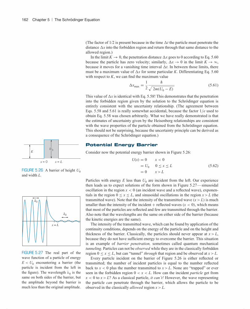
162 Chapter 5 | The Schrodinger Equation
(The factor of 1/2 is present because in the time �t the particle must penetrate thedistance �x into the forbidden region and return through that same distance to theallowed region.)
x = Lx = 0
U0E
FIGURE 5.26 A barrier of height U0
and width L.
In the limit K → 0, the penetration distance �x goes to 0 according to Eq. 5.60because the particle has zero velocity; similarly, �x → 0 in the limit K → ∞,because it moves for a vanishing time interval �t. In between those limits, theremust be a maximum value of �x for some particular K. Differentiating Eq. 5.60with respect to K, we can find the maximum value
�xmax = 1
2
−h√2m(U0 − E)
(5.61)
This value of �x is identical with Eq. 5.58! This demonstrates that the penetrationinto the forbidden region given by the solution to the Schrodinger equation isentirely consistent with the uncertainty relationship. (The agreement betweenEqs. 5.58 and 5.61 is really somewhat accidental, because the factor 1/e used toobtain Eq. 5.58 was chosen arbitrarily. What we have really demonstrated is thatthe estimates of uncertainty given by the Heisenberg relationships are consistentwith the wave properties of the particle obtained from the Schrodinger equation.This should not be surprising, because the uncertainty principle can be derived asa consequence of the Schrodinger equation.)
Potential Energy BarrierConsider now the potential energy barrier shown in Figure 5.26:
U(x) = 0 x < 0
= U0 0 ≤ x ≤ L (5.62)
= 0 x > L
Particles with energy E less than U0 are incident from the left. Our experiencethen leads us to expect solutions of the form shown in Figure 5.27—sinusoidaloscillation in the region x < 0 (an incident wave and a reflected wave), exponen-tials in the region 0 ≤ x ≤ L, and sinusoidal oscillations in the region x > L (thetransmitted wave). Note that the intensity of the transmitted wave (x > L) is muchsmaller than the intensity of the incident + reflected waves (x < 0), which meansthat most of the particles are reflected and few are transmitted through the barrier.Also note that the wavelengths are the same on either side of the barrier (becausethe kinetic energies are the same).
x = L
λ0
λ0
FIGURE 5.27 The real part of thewave function of a particle of energyE < U0 encountering a barrier (theparticle is incident from the left inthe figure). The wavelength λ0 is thesame on both sides of the barrier, butthe amplitude beyond the barrier ismuch less than the original amplitude.
The intensity of the transmitted wave, which can be found by application of thecontinuity conditions, depends on the energy of the particle and on the height andthickness of the barrier. Classically, the particles should never appear at x > L,because they do not have sufficient energy to overcome the barrier. This situationis an example of barrier penetration, sometimes called quantum mechanicaltunneling. Particles can not be observed while they are in the classically forbiddenregion 0 ≤ x ≤ L, but can “tunnel” through that region and be observed at x > L.
Every particle incident on the barrier of Figure 5.26 is either reflected ortransmitted; the number of incident particles is equal to the number reflectedback to x < 0 plus the number transmitted to x > L. None are “trapped” or everseen in the forbidden region 0 < x < L. How can the incident particle get fromx < 0 to x > L? As a classical particle, it can’t! However, the wave representingthe particle can penetrate through the barrier, which allows the particle to beobserved in the classically allowed region x > L.

5.6 | Steps and Barriers 163
(b)(a)
GlassAir
FIGURE 5.28 (a) Total internal reflection of light waves at a glass-airboundary. (b) Frustrated total internal reflection. The thicker the airgap, the smaller the probability to penetrate. Note that the light beamdoes not appear in the gap.
This phenomenon of penetration of a forbidden region is a well-known propertyof classical waves. Quantum physics provides a new aspect to this phenomenon byassociating a particle with the wave, and thus allowing a particle to pass througha classically forbidden region. An example of the penetration effect for classicalwaves occurs for total internal reflection∗ of light waves. Figure 5.28a shows alight beam in glass incident on a boundary with air. The beam is totally reflectedin the glass. However, if a second piece of glass is brought close to the first, asin Figure 5.28b, the beam can appear in the second piece of glass. This effect iscalled frustrated total internal reflection. The intensity of the beam in the secondpiece, represented by the widths of the arrows in Figure 5.28b, decreases rapidlyas the thickness of the gap increases.
Just like our unobservable quantum wave, which penetrates a few wavelengthsinto the forbidden region, an unobservable light wave of exponentially decreasingamplitude, the evanescent wave, penetrates into the air even when the light waveundergoes total reflection in the glass. The evanescent wave carries no energyaway from the interface, so it cannot be directly observed in the air, but it can beobserved in another medium such as a second piece of glass placed close to thefirst. Evanescent waves have applications in microscopy, where they enable theproduction of images of individual molecules. (a)
Attractivenuclear potential
Repulsive Coulombpotential
Energy of alphaparticleE
(b)
FIGURE 5.29 (a) A nuclear poten-tial energy barrier is penetrated byan alpha particle of energy E. (b) Arepresentation of the real part of thewave function of the alpha particle.The probability to penetrate the bar-rier depends strongly on the energy ofthe alpha particle.
Although the potential energy barrier of Figure 5.26 is rather artificial, thereare many practical examples of quantum tunneling:
1. Alpha Decay. An atomic nucleus consists of protons and neutrons in aconstant state of motion; occasionally these particles form themselves into anaggregate of two protons and two neutrons, called an alpha particle. In oneform of radioactive decay, the nucleus can emit an alpha particle, which canbe detected in the laboratory. However, in order to escape from the nucleusthe alpha particle must penetrate a barrier of the form shown in Figure 5.29.The probability for the alpha particle to penetrate the barrier, and be detectedin the laboratory, can be computed based on the energy of the alpha particle
∗Total internal reflection occurs when a light beam is incident on a boundary between two substances,such as glass and air, from the side with the higher index of refraction. If the angle of incidence insidethe glass exceeds a certain critical value, the light beam is totally reflected back into the glass.

164 Chapter 5 | The Schrodinger Equation
and the height and thickness of the barrier. The decay probability can bemeasured in the laboratory, and it is found to be in excellent agreement withthe value obtained from a quantum-mechanical calculation based on barrierpenetration.
2. Ammonia Inversion. Figure 5.30 is a representation of the ammonia moleculeNH3. If we were to try to move the nitrogen atom along the axis of the molecule,toward the plane of the hydrogen atoms, we find repulsion caused by the threehydrogen atoms, which produces a potential energy of the form shown inFigure 5.31. According to classical mechanics, unless we give the nitrogenatom sufficient energy, it should not be able to surmount the barrier and appearon the other side of the plane of hydrogens. According to quantum mechanics,the nitrogen can tunnel through the barrier and appear on the other side of themolecule. In fact, the nitrogen atom actually tunnels back and forth with afrequency in excess of 1010 oscillations per second.
3. The Tunnel Diode. A tunnel diode is an electronic device that uses thephenomenon of tunneling. Schematically, the potential energy of an electronin a tunnel diode can be represented by Figure 5.32. The current that flowsthrough the device is produced by electrons tunneling through the barrier.The rate of tunneling, and therefore the current, can be regulated merely bychanging the height of the barrier, which can be done with an applied voltage.
H
H H
N
FIGURE 5.30 A schematic dia-gram of the ammonia molecule.The Coulomb repulsion of thethree hydrogens establishes a bar-rier against the nitrogen atommoving to a symmetric position(shown in dashed lines) on theopposite side of the plane ofhydrogens.
0Distance from plane of hydrogens
Pot
enti
al e
nerg
yof
nit
roge
n
Equilibriumpositions
Groundstate
energy
Potentialenergybarrier
FIGURE 5.31 The potential en-ergy seen by the nitrogen atomin an ammonia molecule. Thenitrogen can penetrate the barrierand move from one equilibriumposition to another.
Energy ofelectrons
Barrier heightdetermined byapplied voltage
FIGURE 5.32 The potentialenergy barrier seen by an elec-tron in a tunnel diode. Theconductivity of the device isdetermined by the electron’sprobability to penetrate the bar-rier, which depends on theheight of the barrier.

Chapter Summary 165
This can be done rapidly, so that switching frequencies in excess of 109 Hzcan be obtained. Ordinary semiconductor diodes depend on the diffusion ofelectrons across a junction, and therefore operate on much longer time scales(that is, at lower frequencies).
4. The Scanning Tunneling Microscope. Images of individual atoms on thesurface of materials (such as Figure 5.18) can be made with the scanningtunneling microscope. Electrons are trapped in a surface by a potential energybarrier (the work function of the material). When a needlelike probe is placedwithin about 1 nm of the surface (Figure 5.33), electrons can tunnel throughthe barrier between the surface and the probe and produce a current that canbe recorded in an external circuit. The current is very sensitive to the width ofthe barrier (the distance from the probe to the surface). In practice, a feedbackmechanism keeps the current constant by moving the tip up and down. Themotion of the tip gives a map of the surface that reveals details smallerthan 0.01 nm, about 1/100 the diameter of an atom! For the development ofthe scanning tunneling microscope, Gerd Binnig and Heinrich Rohrer wereawarded the 1986 Nobel Prize in physics.
Path ofprobe tip
Probe
Electroncloud
Atomon
surface
FIGURE 5.33 In a scanning tunnel-ing microscope, a needlelike probe isscanned over a surface. The probe ismoved vertically so that the distancebetween the probe and the surfaceremains constant as the probe scanslaterally.
Chapter Summary
Section
Time-independentSchrodingerequation
−−h2
2m
d2ψ
dx2+ U(x)ψ(x) = Eψ(x) 5.3
Time-dependentSchrodingerequation
(x, t) = ψ(x)e−iωt 5.3
Probability density P(x) = |ψ(x)|2 5.3
Normalizationcondition
∫ +∞−∞ |ψ(x)|2 dx = 1 5.3
Probability ininterval x1 to x2
P(x1: x2) = ∫ x2x1
|ψ(x)|2 dx 5.3
Average orexpectation valueof f (x)
[f (x)]av = ∫ +∞−∞ |ψ(x)|2f (x) dx 5.3
Constant potentialenergy, E > U0
ψ(x) = A sin kx + B cos kx,
k = √2m(E − U0)/
−h2
5.4
Constant potentialenergy, E < U0
ψ(x) = Aek′x + Be−k′x,
k′ = √2m(U0 − E)/−h2
5.4
Section
Infinite potentialenergy well
ψn(x) =√
2
Lsin
nπx
L,
En = h2n2
8mL2(n = 1, 2, 3, . . .)
5.4
Two-dimensionalinfinite well
ψ(x, y) = 2
Lsin
nxπx
Lsin
nyπy
L
E = h2
8mL2(n2
x + n2y)
5.4
Simple harmonicoscillator groundstate
ψ(x) = (mω0/−hπ)1/4 e−(
√km/2−h)x2
5.5
Simple harmonicoscillator energies
En = (n + 12 )−hω0 (n = 0, 1, 2, . . .) 5.5
Potential energystep, E > U0
ψ0(x < 0) = A sin k0x + B cos k0xψ1(x > 0) = C sin k1x + D cos k1x
5.6
Potential energystep, E < U0
ψ0(x < 0) = A sin k0x + B cos k0xψ1(x > 0) = Cek1x + De−k1x
5.6

166 Chapter 5 | The Schrodinger Equation
Questions
1. Newton’s laws can be solved to give the future behavior ofa particle. In what sense does the Schrodinger equation alsodo this? In what sense does it not?
2. Why is it important for a wave function to be normalized? Isan unnormalized wave function a solution to the Schrodingerequation?
3. What is the physical meaning of∫ +∞−∞ |ψ |2dx = 1 ?
4. What are the dimensions of ψ(x)? Of ψ(x, y)?5. None of the following are permitted as solutions of the
Schrodinger equation. Give the reasons in each case.
(a) ψ(x) = A cos kx x < 0ψ(x) = B sin kx x > 0
(b) ψ(x) = Ax−1e−kx − L ≤ x ≤ L(c) ψ(x) = A sin−1 kx(d) ψ(x) = A tan kx x > 0
6. What happens to the probability density in the infinite wellwhen n → ∞? Is this consistent with classical physics?
7. How would the solution to the infinite potential energy wellbe different if the well extended from x = x0 to x = x0 + L,where x0 is a nonzero value of x? Would any of the measur-able properties be different?
8. How would the solution to the one-dimensional infinitepotential energy well be different if the potential energywere not zero for 0 ≤ x ≤ L but instead had a constant valueU0? What would be the energies of the excited states? Whatwould be the wavelengths of the standing de Broglie waves?Sketch the behavior of the lowest two wave functions.
9. Assuming a pendulum to behave like a quantum oscilla-tor, what are the energy differences between the quantum
states of a pendulum of length 1 m? Are such differencesobservable?
10. For the potential energy barrier (Figure 5.26), is the wave-length for x > L the same as the wavelength for x < 0? Isthe amplitude the same?
11. Suppose particles were incident on the potential energy stepfrom the positive x direction. Which of the four coefficientsof Eq. 5.56 would be set to zero? Why?
12. The energies of the excited states of the systems we have dis-cussed in this chapter have been exact—there is no energyuncertainty. What does this suggest about the lifetime ofparticles in those excited states? Left on its own, will aparticle ever make transitions from one state to another?
13. Explain how the behavior of a particle in a one-dimensionalinfinite well can be considered in terms of standing deBroglie waves.
14. How would you design an experiment to observe barrierpenetration with sound waves? What range of thicknesseswould you choose for the barrier?
15. If U0 were negative in Figure 5.26, how would the wavefunctions appear for E > 0?
16. Does Eq. 5.2 imply that we know the momentum of theparticle exactly? If so, what does the uncertainty principleindicate about our knowledge of its location? How can youreconcile this with our knowledge that the particle must bein the well?
17. Do sharp boundaries and discontinuous jumps of potentialenergy occur in nature? If not, how would our analysis ofpotential energy steps and barriers be different?
Problems
5.1 Behavior of a Wave at a Boundary
1. A ball falls from rest at a height H above a lake. Let y = 0at the surface of the lake. As it falls, it experiences a gravi-tational force −mg. When it enters the water, it experiencesa buoyant force B so the net force in the water is B − mg.(a) Write expressions for v(t) and y(t) while the ball is fallingin air. (b) In the water, let v2(t) = at + b and y2(t) = 1
2 at2 +bt + c where a = (B − mg)/m. Use the continuity condi-tions at the surface of the water to find the constants b and c.
2. A wave has the form y = A cos(2πx/λ + π/3) when x < 0.For x > 0, the wavelength is λ/2. By applying continuityconditions at x = 0, find the amplitude (in terms of A) andphase of the wave in the region x > 0. Sketch the wave,showing both x < 0 and x > 0.
5.2 Confining a Particle
3. The lowest energy of a particle in an infinite one-dimensionalwell is 4.4 eV. If the width of the well is doubled, what is itslowest energy?
4. An electron is trapped in an infinite well of width 0.120 nm.What are the three longest wavelengths permitted for theelectron’s de Broglie waves?
5. An electron is trapped in a one-dimensional region of width0.050 nm. Find the three smallest possible values allowedfor the energy of the electron.
6. What is the minimum energy of a neutron (mc2 = 940 MeV)confined to a region of space of nuclear dimensions(1.0 × 10⁻¹⁴ m)?

Problems 167
5.3 The Schrodinger Equation
7. In the region 0 ≤ x ≤ a, a particle is described bythe wave function ψ1(x) = −b(x2 − a2). In the regiona ≤ x ≤ w, its wave function is ψ2(x) = (x − d)2 − c. Forx ≥ w, ψ3(x) = 0. (a) By applying the continuity conditionsat x = a, find c and d in terms of a and b. (b) Find w in terms ofa and b.
8. A particle is described by the wave functionψ(x) = b(a2 − x2) for −a ≤ x ≤ +a and ψ(x) = 0 forx ≤ −a and x ≥ +a, where a and b are positive real con-stants. (a) Using the normalization condition, find b in termsof a. (b) What is the probability to find the particle atx = +a/2 in a small interval of width 0.010a? (c) What isthe probability for the particle to be found between x = +a/2and x = +a?
9. In a certain region of space, a particle is described by thewave function ψ(x) = Cxe−bx where C and b are real con-stants. By substituting into the Schrodinger equation, findthe potential energy in this region and also find the energy ofthe particle. (Hint: Your solution must give an energy thatis a constant everywhere in this region, independent of x.)
10. A particle is represented by the following wave function:
ψ(x) = 0 x < −L/2
= C(2x/L + 1) − L/2 < x < 0
= C(−2x/L + 1) 0 < x < +L/2
= 0 x >+L/2
(a) Use the normalization condition to find C. (b) Eval-uate the probability to find the particle in an interval ofwidth 0.010L at x = L/4 (that is, between x = 0.245L andx = 0.255L. (No integral is necessary for this calculation.)(c) Evaluate the probability to find the particle betweenx = 0 and x = +L/4. (d) Find the average value of x andthe rms value of x: xrms = √
(x2)av.
5.4 Applications of the Schrodinger Equation
11. A particle in an infinite well is in the ground state with anenergy of 1.26 eV. How much energy must be added to theparticle to reach the second excited state (n = 3)? The thirdexcited state (n = 4)?
12. An electron is trapped in an infinitely deep one-dimensionalwell of width 0.251 nm. Initially the electron occupies then = 4 state. (a) Suppose the electron jumps to the groundstate with the accompanying emission of a photon. Whatis the energy of the photon? (b) Find the energies of otherphotons that might be emitted if the electron takes otherpaths between the n = 4 state and the ground state.
13. Show that Eq. 5.31 gives the value A =√
2/L.14. A particle is trapped in an infinite one-dimensional well
of width L. If the particle is in its ground state, evaluatethe probability to find the particle (a) between x = 0 and
x = L/3; (b) between x = L/3 and x = 2L/3; (c) betweenx = 2L/3 and x = L.
15. A particle is confined between rigid walls separated by adistance L = 0.189 nm. The particle is in the second excitedstate (n = 3). Evaluate the probability to find the particle inan interval of width 1.00 pm located at: (a) x = 0.188 nm;(b) x = 0.031 nm; (c) x = 0.079 nm. (Hint: No integra-tions are required for this problem; use Eq. 5.7 directly.)What would be the corresponding results for a classicalparticle?
16. What is the next level (above E = 50E0) of the two-dimensional particle in a box in which the degeneracyis greater than 2?
17. A particle is confined to a two-dimensional box of length Land width 2L. The energy values are E = (−h2π2/2mL2)(n2
x +n2
y/4). Find the two lowest degenerate levels.18. Show by direct substitution that Eq. 5.39 gives a solution to
the two-dimensional Schrodinger equation, Eq. 5.37. Findthe relationship between kx, ky, and E.
19. A particle is confined to a three-dimensional region ofspace of dimensions L by L by L. The energy levelsare (−h2π2/2mL2)(n2
x + n2y + n2
z ), where nx, ny, and nz areintegers ≥ 1. Sketch an energy level diagram, showing theenergies, quantum numbers, and degeneracies for the lowest10 energy levels.
5.5 The Simple Harmonic Oscillator
20. Using the normalization condition, show that the constant Ahas the value (mω0/
−hπ)1/4 for the one-dimensional simpleharmonic oscillator in its ground state.
21. (a) At the classical turning points ±x0 of the simple harmonicoscillator, K = 0 and so E = U . From this relationship, showthat x0 = (−hω0/k)1/2 for an oscillator in its ground state.(b) Find the turning points in the first and second excitedstates.
22. Use the ground-state wave function of the simple harmonicoscillator to find xav, (x2)av, and �x. Use the normalizationconstant A = (mω0/
−hπ)1/4.23. (a) Using a symmetry argument rather than a calculation,
determine the value of pav for a simple harmonic oscillator.(b) Conservation of energy for the harmonic oscillator canbe used to relate p2 to x2. Use this relation, along withthe value of (x2)av from Problem 22, to find (p2)av for theoscillator in its ground state. (c) Using the results of parts aand b, show that �p = √−hω0m/2.
24. The ground state energy of an oscillating electron is 1.24 eV.How much energy must be added to the electron to move itto the second excited state? The fourth excited state?
25. Compare the probabilities for an oscillating particle in itsground state to be found in a small interval of width dx atthe center of the well and at the classical turning points.

168 Chapter 5 | The Schrodinger Equation
5.6 Steps and Barriers
26. Find the value of K at which Eq. 5.60 has its maximumvalue, and show that Eq. 5.61 is the maximum value of �x.
27. For a particle with energy E < U0 incident on the potentialenergy step, use ψ0 and ψ1 from Eqs. 5.57, and evaluate theconstants B and D in terms of A by applying the boundaryconditions at x = 0.
28. Using the wave functions of Eq. 5.55 for the potential energystep, apply the boundary conditions of ψ and dψ/dx to findB′ and C′ in terms of A′, for the potential step when particlesare incident from the negative x direction. Evaluate the ratios|B′|2/|A′|2 and |C′|2/|A′|2 and interpret.
29. (a) Write down the wave functions for the three regionsof the potential energy barrier (Figure 5.26) for E < U0.You will need six coefficients in all. Use complex expo-nential notation. (b) Use the boundary conditions at x = 0and at x = L to find four relationships among the six coeffi-cients. (Do not try to solve these relationships.) (c) Supposeparticles are incident on the barrier from the left. Whichcoefficient should be set to zero? Why?
30. Repeat Problem 29 for the potential energy barrier whenE > U0, and sketch a representative probability density thatshows several cycles of the wave function. In your sketch,make sure the amplitude and wavelength in each regionaccurately describe the situation.
General Problems
31. An electron is trapped in a one-dimensional well of width0.132 nm. The electron is in the n = 10 state. (a) Whatis the energy of the electron? (b) What is the uncertaintyin its momentum? (Hint: Use Eq. 4.10.) (c) What is theuncertainty in its position? How do these results change asn → ∞? Is this consistent with classical behavior?
32. Sketch the form of a possible solution to the Schrodingerequation for each of the potential energies shown inFigure 5.34. The potential energies go to infinity at theboundaries. In each case show several cycles of the wavefunction. In your sketches, pay attention to the continu-ity conditions (where applicable) and to changes in thewavelength and amplitude.
33. Show that the average value of x2 in the one-dimensionalinfinite potential energy well is L2(1/3 − 1/2n2π2).
34. Use the result of Problem 33 to show that, for the infi-nite one-dimensional well, defining �x = √
(x2)av − (xav)2
gives �x = L√
1/12 − 1/2π2n2.35. (a) In the infinite one-dimensional well, what is
pav? (Use a symmetry argument.) (b) What is (p2)av? [Hint:
What is (p2/2m)av?] (c) Defining �p = √(p2)av − (pav)
2,show that �p = hn/2L.
E
E
E
FIGURE 5.34 Problem 32.
36. The first excited state of the harmonic oscillator has a wavefunction of the form ψ(x) = Axe−ax2
. Follow the methodoutlined in Section 5.5 to find a and the energy E. Find theconstant A from the normalization condition.
37. Using the normalization constant A from Problem 20 andthe value of a from Eq. 5.49, evaluate the probability tofind an oscillator in the ground state beyond the classicalturning points ±x0. This problem cannot be solved in closed,analytic form. Develop an approximate, numerical methodusing a graph, calculator, or computer. Assume an elec-tron bound to an atomic-sized region (x0 = 0.1 nm) with aneffective force constant of 1.0 eV/nm2.
38. A two-dimensional harmonic oscillator has energy E =−hω0(nx + ny + 1), where nx and ny are integers beginningwith zero. (a) Justify this result based on the energy ofthe one-dimensional oscillator. (b) Sketch an energy-leveldiagram similar to Figure 5.21, showing the lowest 4 energylevels. For each level, show the value of E (in units of−hω0), the quantum numbers nx and ny, and the degener-acy. (c) Show that the degeneracy of each level is equal tonx + ny + 1.