Modern Database Systems - Lecture 02

Modern Database Systems Lecture 2

Aristides Gionis Michael Mathioudakis

T.A.: Orestis Kostakis

Spring 2016

logistics

2

• assignment 1 is up • cowbook available at learning center beta, otakaari 1 x •  if you do not have access to the lab, provide Aalto username or email today!! •  if you do not have access at mycourses, i will post material (slides and assignments) also at http://michalis.co/moderndb/

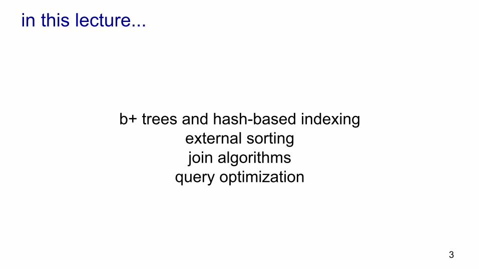
in this lecture...

b+ trees and hash-based indexing external sorting join algorithms

query optimization

3

b+ trees

b+ trees

5

leaf nodes contain data-entries

sequentially linked each node stored in one page

data entries can be any one of the three alternative types type 1: data records; type 2: (k, rid); type 3: (k, rids)

at least 50% capacity - except for root!

non-leaf nodes index entries

used to direct search

in the examples that follow... alternative 2 is used

all nodes have between d and 2d key entries d is the order of the tree

b+ trees

6



P 0 K 1 P 1 K 2 P 2 K m P m

k* < K1 K1 ≤ k* < K2 Km ≤ k*


sequentially linked

closer look at non-leaf nodes

search key values pointers

b+ trees

7

most widely used index

search and updates at logFN cost (cost = pages I/O) F = fanout (num of pointers per index node); N = num of leaf pages

efficient equality and range queries




sequentially linked

example b+ tree - search

search begins at root, and key comparisons direct it to a leaf search for 5*; search for all data entries >= 24*

root

17 24 30

2* 3* 5* 7* 14* 16* 19* 20* 22* 24* 27* 29* 33* 34* 38* 39*

13

8

inserting a data entry

1.  find correct leaf L 2.  place data entry onto L

a.  if L has enough space, done! b.  else must split L into L and L2

•  redistribute entries evenly •  copy up the middle key to parent of L •  insert entry pointing to L2 to parent of L

9

the above happens recursively when index nodes are split, push up middle key

splits grow the tree

root split increases height

example b+ tree

insert 8*

root

17 24 30

2* 3* 5* 7* 14* 16* 19* 20* 22* 24* 27* 29* 33* 34* 38* 39*

13

10

middle key is copied up (and continues to appear in the leaf)

split!

5

≥ 5 < 5

5 24 30

17

13

middle key is pushed up

≥ 17 < 17 split parent node!

L

2* 3* 5* 7* 8*

L L2

example b+ tree

insert 8*

root

17 24 30

2* 3* 5* 7* 14* 16* 19* 20* 22* 24* 27* 29* 33* 34* 38* 39*

13

11

2* 3*

17

24 30

14* 16* 19* 20* 22* 24* 27* 29* 33* 34* 38* 39*

13 5

7* 5* 8*

deleting a data entry

12

inverse of insertion

re-distribute entries & (maybe) merge nodes

vs split nodes & re-distribute entries

when nodes are less than half-full

when nodes overflow

remove data entry add data entry vs

deletion insertion

b+ trees in practice typical order d = 100, fill-factor = 67%

average fan-out 133

typical capacities: for height 4: 1334 = 312,900,700 records

for height 3: 1333 = 2,352,637 records

can often hold top levels in main memory level 1: 1 page = 8KBytes

level 2: 133 pages = 1MByte level 3: 17,689 pages = 133 MBytes

13

hash-based indexes

hash-based index

the index supports equality queries does not support range queries static and dynamic variants exist 15

data entries organized in M buckets bucket = a collection of pages

the data entry for record

with search key value key is assigned to bucket

h(key) mod M

hash function h(key) e.g., h(key) = α key + β

h(key) mod M

key h

0

1

2

M-1

...

buckets

static hashing

number of buckets is fixed

start with one page per bucket

allocated sequentially, never de-allocated can use overflow pages

16

h(key) mod M

key h

0

1

2

M-1

...

buckets

static hashing

drawback long overflow chains can degrade performance

dynamic hashing techniques

adapt index to data size extendible and linear hashing

17

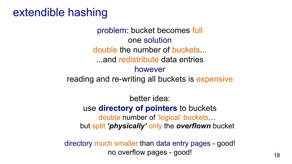
extendible hashing problem: bucket becomes full

one solution double the number of buckets... ...and redistribute data entries

however reading and re-writing all buckets is expensive

better idea:

use directory of pointers to buckets double number of ‘logical’ buckets…

but split ‘physically’ only the overflown bucket

directory much smaller than data entry pages - good! no overflow pages - good! 18

example

2

2

2

2

local depth

2

global depth

directory

00011011

data entries

bucket A

bucket B

bucket C

bucket D

4* 12* 32* 16*

1* 5* 21* 13*

10*

15* 7* 19*

directory is array of size M = 4 = 22

to find bucket for r, take last 2 # bits of h(r) h(r) = key

e.g., if h(r) = 5 = binary 101

it is in bucket pointed to by 01

global depth = 2 = min. bits enough to enumerate buckets

local depth

= min bits to identify individual bucket = 2

19

insertion

2

2

2

2

local depth

2

global depth

directory

00011011

data entries

bucket A

bucket B

bucket C

bucket D

4* 12* 32* 16*

1* 5* 21* 13*

10*

15* 7* 19*

try to insert entry to corresponding bucket

if necessary, double the directory i.e., when for split bucket local depth > global depth

20

when directory doubles, increase global depth +1

if bucket is full, increase +1 local depth

and split bucket (allocate new bucket, re-distribute)

example insert record with h(r) = 20 = binary 10100 è bucket A

split bucket A ! allocate new page,

redistribute according to modulo 2M = 8

3 least significant bits

we’ll have more than 4 buckets now,

so double the directory!

00011011

2

2

2

2

2

local depth

global depth

directory

bucket A

bucket B

bucket C

bucket D

data entries

4* 12* 32* 16*

1* 5* 21* 13*

10*

15* 7* 19*

21

global depth

2

example

3

2

2

2

2

2

local depth 3

2

2

2

3

directory

001

4* 12* 20* bucket A2split image of A

000

010011

bucket A

bucket B

bucket C

bucket D

32* 16*

1* 5* 21* 13*

10*

15* 7* 19*

100101110111

22

split bucket A and redistribute entries

update local depth double the directory update global depth

update pointers

notes

20 = binary 10100 last 2 bits (00) tell us r belongs in A or A2

last 3 bits needed to tell which

global depth of directory number of bits enough to determine which bucket any entry belongs to

local depth of a bucket number of bits enough to determine if an entry belongs to this bucket

when does bucket split cause directory doubling? before insert, local depth of bucket = global depth

23

example

34* 12* 20* bucket A2

000001010011

3

3

2

2

2

local depth

global depth

directory

bucket A

bucket B

bucket C

bucket D

32* 16*

1* 5* 21* 13*

10*

15* 7* 19*

100101110111

insert h(r) = 17

split bucket B

000001010011

3 3

global depth

directory

bucket B1* 17*

100101110111

3bucket B25* 21* 13*

24

other buckets not shown

comments on extendible hashing if directory fits in memory,

equality query answered in one disk access answered = retrieve rid

directory grows in spurts

if hash values are skewed, it might grow large

delete: reverse algorithm empty bucket can be merged with its ‘split image’

when can the directory be halved? when all directory elements point to same bucket as their ‘split image’

25

indexes in SQL

create index

CREATE INDEX indexbON students (age, grade)USING BTREE;

CREATE INDEX indexhON students (age, grade)USING HASH;

DROP INDEX indexhON student;

27

28

external sorting

the sorting problem setting

a relation R, stored over N disk pages 3≤B<N pages available in memory (buffer pages)

task

sort records of R and store result on disk sort by a function of record field values f(r)

why

application need records ordered part of join implementation (soon...)

29

sorting with 3 buffer pages

2 phases

30

1

2

N

input relation R

N p

ages

sto

red

on d

isk

output sorted R

f(r)

N pages stored on disk

buffer (memory used by dbms)

sorting with 3 buffer pages - first phase

31

1

2

N

input relation R

N p

ages

sto

red

on d

isk

pass 0: output N runs run: sorted sub-file

after first phase: one run is one page how: load one page at a time,

sort it in-memory, output to disk

run #1

run #2

run #N

only 1 buffer page needed for first phase

output N runs

run #1

...

run #N/2

sorting with 3 buffer pages - second phase

32

input relation R

N p

ages

sto

red

on d

isk

run #1

run #2

run #(N-1)

run #N

pass 1,2,...: halve the runs how: scan pairs of runs, each in own page,

merge in-memory into a new run, output to disk

input page 1

input page 2

output page


output half runs

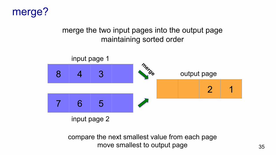
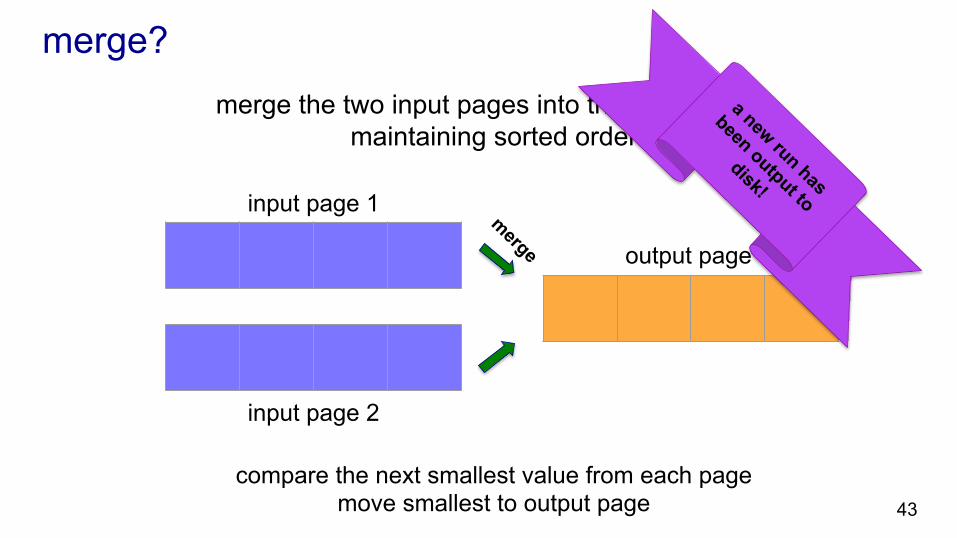
merge?

33

input page 1

input page 2

output page 8 4 3 1

7 6 5 2

merge the two sorted input pages into the output page

maintaining sorted order

compare the next smallest value from each page move smallest to output page

values f(r)

merge?

34

input page 1

input page 2

output page 8 4 3

7 6 5 2 1

merge the two input pages into the output page maintaining sorted order


merge?

35

input page 1

input page 2

output page 8 4 3

7 6 5 2 1



merge?

36

input page 1

input page 2

output page 8 4

7 6 5 3 2 1



merge?

37

input page 1

input page 2

output page 8

7 6 5 4 3 2 1



output page is full, what do we do?

write it to disk!

merge?

38

input page 1

input page 2

output page 8

7 6 5



merge?

39

input page 1

input page 2

output page 8

7 6 5



merge?

40

input page 1

input page 2

output page 8

7 6 5



merge?

41

input page 1

input page 2

output page 8

7 6 5



input page is empty! what do we do?

if the input run has more pages, load

next one

merge?

42

input page 1

input page 2

output page

8 7 6 5



merge?

43

input page 1

input page 2

output page



sorting with 3 buffer pages - second phase

44

input relation R

N p

ages

sto

red

on d

isk N

pages stored on disk

run #1

run #2

run #(N-1)

run #N

pass 1,2,...: halve the runs after log2N passes...

we are done!

input page 1

input page 2

output page

output sorted R

f(r)

sorting with B buffer pages

45

1

2

N

input relation R

N p

ages

sto

red

on d

isk

output sorted R

f(r)


page #B

page #1

page #2

page #(B-1)

same approach

...

sorting with B buffer pages - first phase

46

1

2

N

input relation R

N p

ages

sto

red

on d

isk

output sorted R


...

pass 0: output [N/B] runs how: load R to memory in chunks

of B pages, sort in-memory, output to disk

run #1

run #2

run #[N/B]

page #B

page #1

page #2

page #(B-1)

sorting with B buffer pages - second phase

47

input relation R

N p

ages

sto

red

on d

isk

output sorted R

f(r)


output page

pass 1,2,...: merge runs in groups of B-1

...

input page #1

input page #2

input page #(B-1)

run #1

run #2

run #[N/B]

sorting with B buffer pages

48

1

2

N

input relation R

N p

ages

sto

red

on d

isk

output sorted R

f(r)


output page

how many passes in total? let N1 = [N/B]

total number of passes = 1 + [logB-1(N1)]

...

input page #1

input page #2

input page #(B-1)

phase 1 phase 2

sorting with B buffer

49

1

2

N

input relation R

N p

ages

sto

red

on d

isk

output sorted R

f(r)


output page

how many pages I/O per pass?

...

input page #1

input page #2

input page #(B-1)

2N: N input, N output

sql joins

50

joins

so far, we have seen queries that operate on a single relation

but we can also have queries that

combine information from two or more relations

51

joins

sid name username age

53666 Sam Jones jones 22

53688 Alice Smith smith 22

53650 Jon Edwards jon 23

students

sid points grade

53666 92 A

53650 65 C

dbcourse

52

SELECT * FROM students S, dbcourse C WHERE S.sid = C.sid

what does this compute?

S.sid S.name S.username C.age C.sid C.points C.grade

53666 Sam Jones jones 22 53666 92 A

53650 Jon Edwards jon 23 53650 65 C

joins

53


S record #1 C record #1



... ...




... ...

intuitively... take all pairs of records from S and C

(the “cross product” S x C)

keep only records that satisfy WHERE condition

joins

54





... ...




... ...



(the “cross product” S x C)

output join result

S S.sid=C.sid C

joins

55




(the “cross product” S x C) S record #1 C record #2


output join result

S S.sid=C.sid C

expensive to materialize!

in what follows...

algorithms to compute joins without materializing cross product

56


assuming WHERE condition is equality condition as in the example

assumption is not essential, though

join algorithms

57

the join problem

input relation R: M pages on disk, pR records per page relation S: N pages on disk, pS records per page

M ≤ N

output

58

R R.a=S.b S

if there is enough memory...

load both relations in memory

59

R

S

M pages

N pages

output pages

in-memory for each record r in R for each record s in S if r.a = s.b: store (r, s) in output pages output

I/O cost (ignoring final output cost)

M + N pages

not necessarily to disk

we only have to scan each relation once

output

page-oriented simple nested loops join

60

1 input page output page

join using 3 memory (buffer) pages

R

S

1 input page

for each page P of R for each page Q of S compute P join Q; store in output page

output

I/O cost (pages) M + M * N

outer relation

inner relation

R is scanned once S is scanned M times

block nested loops join

61

B - 2 input pages output page

join using B memory (buffer) pages

R

S

1 input page

for each block P of (B-2) pages of R for each page Q of S compute P join Q; store in output page

output

I/O cost (pages) M + [M/(B-2)] * N

outer relation

inner relation

R is scanned once S is scanned M/(B-2) times

index nested loop join relation S has an index on the join attribute

use one page to make a pass over R use index to retrieve only matching records of S

62

1 input page output page

R

S

1 input page

output

outer relation

inner relation

for each record r of R for each record s of S with s.b = r.a // query index add (r,s) to output

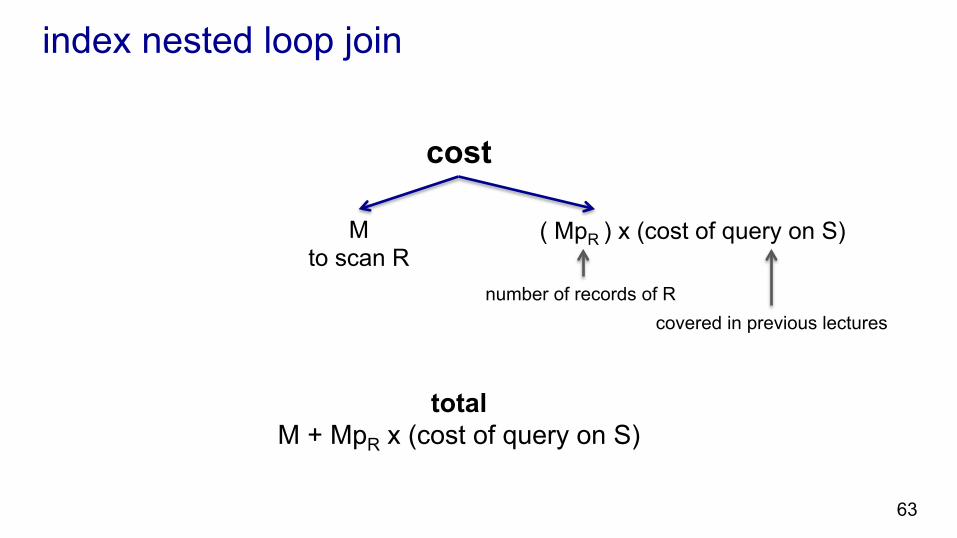
index nested loop join

cost

63

M to scan R

( MpR ) x (cost of query on S)

number of records of R covered in previous lectures

total M + MpR x (cost of query on S)

sort-merge join

two phases sort and merge

sort

R and S on the join attribute using external sort algorithm

cost O(nlogn), n: number of relation pages

merge sorted R and S

64

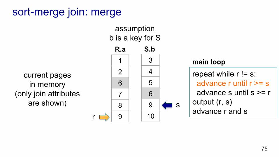
sort-merge join: merge

65

sorted R

sorted S

1 input page

output page

1 input page

output

(B - 3) other buffer pages


66

1 2 6 7 8 9

current pages in memory

(only join attributes are shown)

3 4 5 6 9

10

R.a S.b r s main loop

repeat while r != s: advance r until r >= s advance s until s >= r output (r, s) advance r and s

assumption b is a key for S


67

1 2 6 7 8 9



3 4 5 6 9

10

R.a S.b

r s main loop




68

1 2 6 7 8 9



3 4 5 6 9

10

R.a S.b

r

s main loop




69

1 2 6 7 8 9



3 4 5 6 9

10

R.a S.b

r s

main loop




70

1 2 6 7 8 9



3 4 5 6 9

10

R.a S.b

r s

main loop




71

1 2 6 7 8 9



3 4 5 6 9

10

R.a S.b

r s

main loop




72

1 2 6 7 8 9



3 4 5 6 9

10

R.a S.b

r s


main loop



73

1 2 6 7 8 9



3 4 5 6 9

10

R.a S.b

r s


main loop



74

1 2 6 7 8 9



3 4 5 6 9

10

R.a S.b

r s


main loop



75

1 2 6 7 8 9



3 4 5 6 9

10

R.a S.b

r s


main loop



76

1 2 6 7 8 9



3 4 5 6 9

10

R.a S.b

r s


main loop



77

13 14 15 17 19 23



3 4 5 6 9

10

R.a S.b r


main loop


s

new page for R!


78

13 14 15 17 19 23



3 4 5 6 9

10

R.a S.b r


main loop


s

cost for merge M + N


79

13 14 15 17 19 23



3 4 5 6 9

10

R.a S.b r


main loop


s

cost for merge M + N

what if this assumption does not hold?


80

sorted R sorted S

the pages of sorted R and S

join attribute is not key

on either relation


81

sorted R sorted S



on either relation

parts of R and S with same join attribute value

must output cross product of these parts

R.a = 15

R.a = 20

S.b = 15

S.b = 20


82

sorted R sorted S



on either relation

modify algorithm to perform join over these areas e.g., page-oriented simple nested loops

R.a = 15

R.a = 20

S.b = 15

S.b = 20 for that algorithm, worst case cost

is M + MN

two phases partition and probe

partition

each relation into partitions using the same hash function

on the join attribute

probe join the corresponding partitions

83

hash join

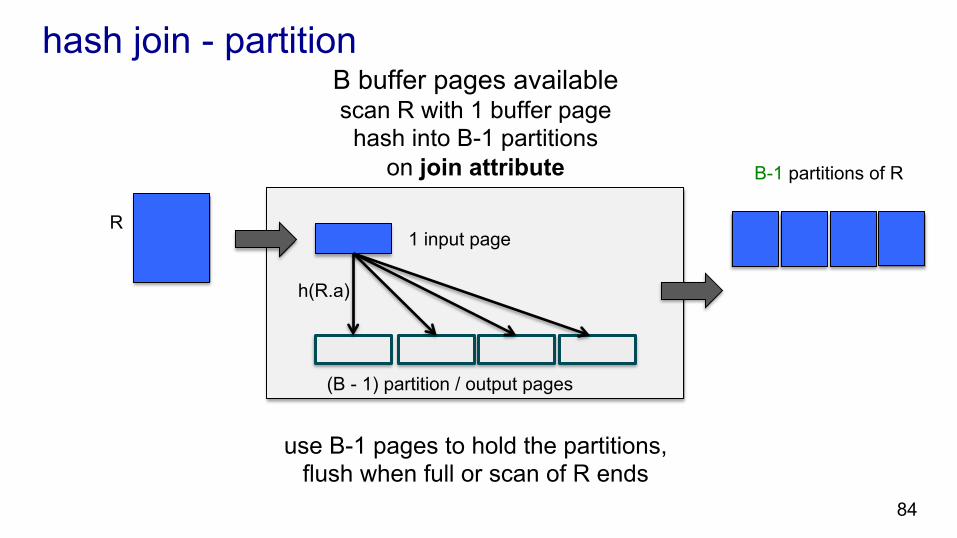
hash join - partition

84

1 input page

(B - 1) partition / output pages

h(R.a)

R

B-1 partitions of R

use B-1 pages to hold the partitions, flush when full or scan of R ends

B buffer pages available scan R with 1 buffer page hash into B-1 partitions

on join attribute

hash join - partition

85

1 input page

(B - 1) partition / output pages

h(S.b)

S

B-1 partitions of R

B-1 partitions of S

B buffer pages available scan S with 1 buffer page hash into B-1 partitions

on join attribute

use B-1 pages to hold the partitions, flush when full or scan of S ends

hash join - probe

86

B-2 input pages

output page

1 input page

output

k-th partition of R

k-th partition of S

B buffer pages available load k-th partition of R into memory

(assuming it fits in B-2 pages)

scan k-th partition of S one page at a time; for each record of S, probe the partition

of R for matching records; store matches in output page;

flush when full or done

holds when size of each partition fits in B-2 pages

approximately B-2 > M / (B - 1)

B > √M

variant re-partition the partition of

R in-memory with hash function h2,

probe using h2

hash join cost

87

partition phase read and write each relation once

2M + 2N

probing phase read each partition once (final output cost ignored)

M + N

total 3M + 3N

a few words on query optimization

88

query optimization

once we submit a query the dbms is responsible for

efficient computation

the same query can be executed in many ways

each is an ‘execution plan’ or ‘query evaluation plan’

89

example select *from studentswhere sid = 100

90

students

σsid = 100

(scan)

(on-the-fly)

execution plan

annotated relational algebra tree

access path how we retrieve data from the relation: scan or index?

algorithm used by operator

students

σsid = 100

(b+ tree index stud_btree on sid)

(query index stud_btree)

another execution plan

example select *from students S, dbcourse Cwhere S.sid = C.sid

91

students S (scan)

execution plan

C.sid = S.sid

dbcourse C (scan)

(block-nested -loops)

another execution plan

students S (index stud_btree)

C.sid = S.sid

dbcourse C (scan)

(index-nested-loops)

which plan to choose?

dbms estimates cost for a number of execution plans (not all possible plans, necessarily!)

the estimates follow the cost analysis

we presented earlier

dbms picks the execution plan with minimum estimated cost

92

summary

93

summary •  commonly used indexes •  B+ tree

•  most commonly used •  supports efficient equation and range queries

•  hash-based indexes • extendible hashing uses directory, not overflow pages

•  external sorting •  joins •  query optimization

94

tutorial

next week

95

references ●  “cowbook”, database management systems, by ramakrishnan and gehrke ●  “elmasri”, fundamentals of database systems, elmasri and navathe ●  other database textbooks

96

credits some slides based on material from database management systems, by ramakrishnan and gehrke

backup slides

97

b+ tree - deletion

98

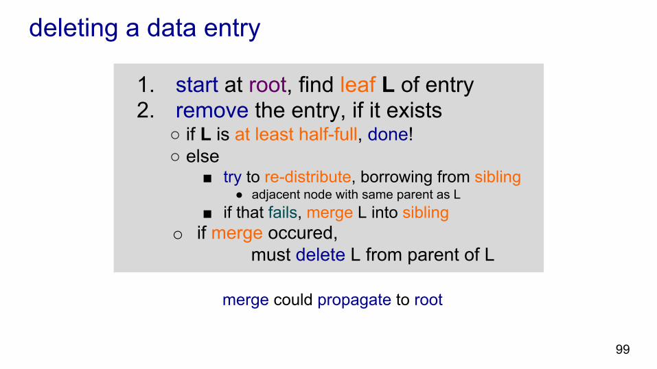
deleting a data entry

1.  start at root, find leaf L of entry 2.  remove the entry, if it exists

○  if L is at least half-full, done! ○ else

■  try to re-distribute, borrowing from sibling ●  adjacent node with same parent as L

■  if that fails, merge L into sibling o  if merge occured,

must delete L from parent of L

99

merge could propagate to root

example b+ tree

delete 19* 2* 3*

root 17

24 30

14* 16* 19* 20* 22* 24* 27* 29* 33* 34* 38* 39*

13 5

7* 5* 8*

100

2* 3*

17

24 30

14* 16* 20* 22* 24* 27* 29* 33* 34* 38* 39*

13 5

7* 5* 8*

example b+ tree

delete 20* 2* 3*

root 17

24 30

14* 16* 20* 22* 24* 27* 29* 33* 34* 38* 39*

13 5

7* 5* 8*

101

2* 3*

17

24 30

14* 16* 22* 24* 27* 29* 33* 34* 38* 39*

13 5

7* 5* 8*

occupancy below 50%, redistribute!

example b+ tree

delete 20* 2* 3*

root 17

24 30

14* 16* 20* 22* 24* 27* 29* 33* 34* 38* 39*

13 5

7* 5* 8*

102

2* 3*

17

27 30

14* 16* 22* 27* 29* 33* 34* 38* 39*

13 5

7* 5* 8*

occupancy below 50%, redistribute!

24*

middle key is copied up!

example b+ tree

delete 24* 2* 3*

root 17

27 30

14* 16* 22* 24* 27* 29* 33* 34* 38* 39*

13 5

7* 5* 8*

103 occupancy below 50%, merge!

2* 3*

17

27 30

14* 16* 22* 27* 29* 33* 34* 38* 39*

13 5

7* 5* 8*

example b+ tree

delete 24* 2* 3*

root 17

27 30

14* 16* 22* 24* 27* 29* 33* 34* 38* 39*

13 5

7* 5* 8*

104 occupancy below 50%, merge!

2* 3*

17

27 30

14* 16* 22* 27* 29* 33* 34* 38* 39*

13 5

7* 5* 8*

delete from parent! reverse of copying up

example b+ tree

delete 24* 2* 3*

root 17

27 30

14* 16* 22* 24* 27* 29* 33* 34* 38* 39*

13 5

7* 5* 8*

105

2* 3*

17

30

14* 16* 22* 27* 29* 33* 34* 38* 39*

13 5

7* 5* 8*


example b+ tree

delete 24* 2* 3*

root 17

27 30

14* 16* 22* 24* 27* 29* 33* 34* 38* 39*

13 5

7* 5* 8*

106

2* 3*

17

30

14* 16* 22* 27* 29* 33* 34* 38* 39*

13 5

7* 5* 8*


example b+ tree

delete 24* 2* 3*

root 17

27 30

14* 16* 22* 24* 27* 29* 33* 34* 38* 39*

13 5

7* 5* 8*

107

2* 3*

17

30

14* 16* 22* 27* 29* 33* 34* 38* 39*

13 5

7* 5* 8*

merge children of root! reverse of pushing up

example b+ tree

delete 24* 2* 3*

root 17

27 30

14* 16* 22* 24* 27* 29* 33* 34* 38* 39*

13 5

7* 5* 8*

108

2* 3*

17 30

14* 16* 22* 27* 29* 33* 34* 38* 39*

13 5

7* 5* 8*

merge children of root! reverse of pushing up

example b+ tree

delete 24* 2* 3*

root 17

27 30

14* 16* 22* 24* 27* 29* 33* 34* 38* 39*

13 5

7* 5* 8*

109

2* 3* 7* 14* 16* 22* 27* 29* 33* 34* 38* 39* 5* 8*

30 13 5 17

example b+ tree

13 5 17 20

22

30

14* 16* 17* 18* 20* 33* 34* 38* 39* 22* 27* 29* 21* 7* 5* 8* 3* 2*

during deletion of 24* -- different example

110

left child of root has many entries (full)

can redistribute entries of index nodes pushing through root splitting entry

example b+ tree

13 5

17

20 22 30

14* 16* 17* 18* 20* 33* 34* 38* 39* 22* 27* 29* 21* 7* 5* 8* 3* 2*

during deletion of 24* -- different example

111

left child of root has many entries (full)

can redistribute entries of index nodes pushing through root splitting entry

example b+ tree

13 5

17

20 22 30

14* 16* 17* 18* 20* 33* 34* 38* 39* 22* 27* 29* 21* 7* 5* 8* 3* 2*

112

linear hashing

113

linear hashing

dynamic hashing uses overflow pages; no directory

splits a bucket in round-robin fashion when an overflow occurs

M = 2level: number of buckets at beginning of round pointer next ∈ [0, M) points at next bucket to split

already next - 1 ‘split-image’ buckets appended to original M

114

linear hashing to allocate entries, use

H0(key) = h(key) mod M, or H1(key) = h(key) mod 2M

i.e., level or level+1 least significant bits of h(key)

to allocate bucket for key first use H0(key)

if H0(key) is less than next then it refers to a split bucket

use H1(key) to determine if it refers to original or its split image

115

linear hashing in the middle of a round...

M buckets that existed at the beginning of this round; this is the range of H0

bucket to be split next buckets already split in this round

split image buckets created through splitting of other buckets in this round

if H0(key) is in this range, then must use H1(key) to decide if entry is in split image bucket

> is a directory necessary? 116

linear hashing inserts insert

find bucket by applying H0 / H1 and insert if there is space

if bucket to insert into is full:

add overflow page, insert data entry, split next bucket and increment next

since buckets are split round-robin, long overflow chains don’t develop!

117

example - insert h(r) = 43 on split, H1 is used to redistribute entries

H0

this is for illustration only!

M=4

00

01

10

11

000

001

010

011

actual contents of the linear hashing file

next=0 PRIMARY

PAGES

44* 36* 32*

25* 9* 5*

14* 18* 10* 30*

31* 35* 11* 7*

00

01

10

11

000

001

010

011

next=1

PRIMARY PAGES

44* 36*

32*

25* 9* 5*

14* 18* 10* 30*

31* 35* 11* 7*

OVERFLOW PAGES

43*

00 100

H1 H0 H1

118

Modern Database Systems - Lecture 02

Education

Transcript of Modern Database Systems - Lecture 02