Modern Applied Statistics with S-Plus - Department of ... · 16 Spatial Statistics 89 ... Kernel...
113
Statistics Complements to Modern Applied Statistics with S-Plus Second edition by W. N. Venables and B. D. Ripley Springer (1997). ISBN 0-387-98214-0 17 February 1999 These complements have been produced to supplement the second edition of MASS. They will be updated from time to time. The definitive source is http://www.stats.ox.ac.uk/pub/MASS2/ . c W. N. Venables and B. D. Ripley 1997, 1998, 1999. A licence is granted for personal study and classroom use. Redistribution in any other form is prohibited. Selectable links are in this colour. Selectable URLs are in this colour.
-
Upload
truongcong -
Category
Documents
-
view
213 -
download
0
Transcript of Modern Applied Statistics with S-Plus - Department of ... · 16 Spatial Statistics 89 ... Kernel...

Statistics Complements to
Modern AppliedStatistics with S-Plus
Second edition
by
W. N. Venables and B. D. RipleySpringer (1997). ISBN 0-387-98214-0
17 February 1999
These complements have been produced to supplement the second edition ofMASS. They will be updated from time to time. The definitive source ishttp://www.stats.ox.ac.uk/pub/MASS2/ .
c© W. N. Venables and B. D. Ripley 1997, 1998, 1999. A licence is granted forpersonal study and classroom use. Redistribution in any other form is prohibited.
Selectable links are in this colour.Selectable URLs are in this colour.

i
Introduction
These complements are made available on-line to supplement the book makinguse of extensions to S-PLUS in user-contributed library sections.
The general convention is that material here should be thought of as followingthe material in the chapter in the book, so that new sections are numbered followingthe last section of the chapter, and figures and equations here are numberedfollowing on from those in the book.
All the libraries mentioned are available for Unix and for Windows. Compiledversions for Windows (for both S-PLUS 3.x and 4.x) are available from either ofthe URLs
http://www.stats.ox.ac.uk/pub/SWin/http://lib.stat.cmu.edu/DOS/S/SWin/
Most of the Unix sources are available at
http://lib.stat.cmu.edu/S/
and more specific information is given for the exceptions where these are intro-duced.
There are separate Complements documents for programming and for S-PLUS 4.xavailable from http://www.stats.ox.ac.uk/pub/MASS2/.

ii
Contents
Introduction i
5 Distributions and Data Summaries 1
5.5 Density estimation . . . . . . . . . . . . . . . . . . . . . . . . . 1
5.6 Bootstrap and permutation methods . . . . . . . . . . . . . . . . 8
7 Generalized Linear Models 12
7.1 Functions for generalized linear modelling . . . . . . . . . . . . . 12
7.3 Poisson models . . . . . . . . . . . . . . . . . . . . . . . . . . . 12
7.5 Gamma models . . . . . . . . . . . . . . . . . . . . . . . . . . . 18
9 Non-linear Models 22
9.4 Confidence intervals for parameters . . . . . . . . . . . . . . . . 22
10 Random and Mixed Effects 24
10.3 Linear mixed effects models . . . . . . . . . . . . . . . . . . . . 24
10.4 Non-linear mixed effects models . . . . . . . . . . . . . . . . . . 30
10.5 Using lme with autocorrelated data . . . . . . . . . . . . . . . . 35
11 Modern Regression 37
11.1 Additive models and scatterplot smoothers . . . . . . . . . . . . . 37
11.2 Projection-pursuit regression . . . . . . . . . . . . . . . . . . . . 44
11.4 Neural networks . . . . . . . . . . . . . . . . . . . . . . . . . . . 49
12 Survival Analysis 55
12.1 Estimators of survival curves . . . . . . . . . . . . . . . . . . . . 55
12.6 Non-parametric models with covariates . . . . . . . . . . . . . . 57
13 Multivariate Analysis 62
13.3 Discriminant analysis . . . . . . . . . . . . . . . . . . . . . . . . 62
13.5 Factor analysis . . . . . . . . . . . . . . . . . . . . . . . . . . . 65

Contents iii
14 Tree-based Methods 67
14.4 Library RPart . . . . . . . . . . . . . . . . . . . . . . . . . . . . 67
14.5 Tree-structured survival analysis . . . . . . . . . . . . . . . . . . 79
15 Time Series 86
15.1 Second-order summaries . . . . . . . . . . . . . . . . . . . . . . 86
16 Spatial Statistics 89
16.3 Module S+SPATIALSTATS . . . . . . . . . . . . . . . . . . . . . . 89
17 Classification 93
17.3 Forensic glass . . . . . . . . . . . . . . . . . . . . . . . . . . . . 93
17.4 Cross-validation . . . . . . . . . . . . . . . . . . . . . . . . . . . 101
References 103
Index 106

1
Chapter 5
Distributions and Data Summaries
5.5 Density estimation
Simonoff (1996) provides an excellent overview of methods for both smoothingand density estimation. Bowman & Azzalini (1997) concentrate on providingan introduction to kernel-based methods, with an easy-to-use S-PLUS librarysm 1 This has the unusual ability to compute and plot kernel density estimates ofthree-dimensional and spherical data.
Kernel density estimation is a rather simple and usual rapid procedure (al-though bandwidth selection need not be). More recently there have been a numberof alternative approaches which use very much greater amounts of computation.
Spline fitting to log-densities
There are several closely-related proposals2 to use a univariate density estimatorof the form
f(y) = exp g(y; θ) (5.7)
for a parametric family g(·; θ) of smooth functions, most often splines. The fitcriterion is maximum likelihood, possibly with a smoothness penalty. The ad-vantages of (5.7) is that it automatically provides a non-negative density estimate,and that it may be more natural to consider ‘smoothness’ on a relative rather thanabsolute scale. It is necessary to ensure that the estimated density has unit mass,and this is most conveniently done by taking
f(y) = exp g(y; θ)/∫
exp g(y; θ) dy (5.8)
The library logspline 3 by Charles Kooperberg implements one variant onthis theme by Kooperberg & Stone (1992), although a later version described inStone et al. (1997) is promised to replace it. This uses a cubic spline for g in(5.8), with smoothness controlled not by a penalty (as in smoothing splines) but
1 available from http://www.stats.gla.ac.uk/~adrian/sm andhttp://www.stat.unipd.it/dip/homes/azzalini/SW/Splus/sm.
2 see Simonoff (1996, pp. 67–70, 90–92) for others.3 logsplin on Windows.

5.5 Density estimation 2
by the number of knots selected. There is an AIC-like penalty; the number of theknots is chosen to maximize
n∑i=1
g(yi; θ) − n log∫
exp g(y; θ) dy − a× number of parameters (5.9)
The default value of a is log n (sometimes known as BIC) but this can be setas an argument of logspline.fit . A Newton method is used to maximize thelog-likelihood given the knot positions. The initial knots are selected at quantilesof the data and then deleted one at a time using the Wald criterion for significance.Finally, (5.9) is used to choose one of the knot sequences considered.
eruptions
1 2 3 4 5 6
0.0
0.2
0.4
0.6
0.8
1.0
bootstrap samples of median
3.7 3.8 3.9 4.0 4.1 4.2
05
1015
20
• ••
••
• • •
•
• • • •
• • •• • •• •
• • •
•
• • • •
• • •
Figure 5.12: Histograms and logspline density plots of (left) the Old Faithful eruptionsdata and (right) bootstrap samples of the median of that dataset. Compare with Figures 5.8(on page 182), Figure 9.4 (page 288) and Figure 5.11 (page 188).
We first try out our two running examples:
library(logspline) # logsplin on Windowsattach(faithful)faithful.ls <- logspline.fit(eruptions, lbound=0)x <- seq(1, 6, len=200)truehist(eruptions, nbins=15, xlim=c(1,6), ymax=1.0)lines(x, dlogspline(x, faithful.ls))detach()
truehist(tperm, xlab="diff")tperm.ls <- logspline.fit(tperm)x <- seq(-5, 5, len=200)lines(x, dlogspline(x, tperm.ls))
sres <- c(sort(tperm), 5); yres <- (0:1024)/1024plot(sres, yres, type="S", xlab="diff", ylab="cdf")lines(x, plogspline(x, tperm.ls))
par(pty="s")x <- c(0.0005, seq(0.001, 0.999, 0.001), 0.9995)plot( qt(x, 9), qlogspline(x, tperm.ls),
xlab="Quantiles of t on 9 df", ylab="Fitted quantiles",type="l", xlim=c(-5, 5), ylim=c(-5, 5))
points( qt(ppoints(tperm), 9), sort(tperm) )

5.5 Density estimation 3
The functions dlogspline , plogspline and qlogspline compute the den-sity, CDF and quantiles of the fitted density, so the final plot is a QQ-plot of thedata and the fitted density against the t9 density. The final plot shows that thet9 density is a better fit in the tails; the logspline density estimate always hasexponential tails. (The function logspline.plot will make a simple plot of thedensity, CDF or hazard estimate.)
diff-4 -2 0 2 4
0.0
0.1
0.2
0.3
0.4
diff
cdf
-4 -2 0 2 4
0.0
0.2
0.4
0.6
0.8
1.0
Quantiles of t on 9df
Fitt
ed q
uant
iles
-4 -2 0 2 4
-4-2
02
4
••
•••••
•••••••••••••••••••••••
•••••••••••••••••••••••••••••••••••••••••••••••••••••
••••••••••••••••••••••••••••••••••••••••••••••••
••••••••••••••••••••••••••••••••••••••••••••••••••••••••
•••••••••••••••••••••••••••••••••••••••••••••••••••••••
•••••••••••••••••••••••••••••••••••••••••••••••••••••••••••••
•••••••••••••••••••••••••••••••••
•••••••
••
•
Figure 5.13: Plots of the logspline density estimate of the permutation dataset tperm .The three panels show the histogram with superimposed density estimate, the empiricaland fitted CDFs and QQ–plots of the data and the fitted density against the conventional t9distribution.
We can also explore density plots of the bootstrapped median values frompage 187 (which we recall actually has a discrete distribution).
truehist(res, nbins=nclass.FD(res), ymax=20)x <- seq(3.7, 4.2, len=1000)res.ls <- logspline.fit(res)lines(x, dlogspline(x, res.ls))points(res.ls$knots, dlogspline(res.ls$knots, res.ls))res.ls <- logspline.fit(res, penalty=2)lines(x, dlogspline(x, res.ls), lty=3)points(res.ls$knots, dlogspline(res.ls$knots, res.ls))
Changing the penalty a to the AIC value of 2 has a small effect. The dots showwhere the knots have been placed. (The function logspline.summary showsdetails of the selection of the number of knots.)
The results for the galaxies data are also instructive.
x <- seq(8000, 35000, 200)plot(x, dlogspline(x, logspline.fit(galaxies)), type="l",
xlab="velocity of galaxy", ylab="density")lines(density(galaxies, n=200, window="gaussian",
width=width.SJ(galaxies)), lty=3)
Maximum-likelihood methods and hence logspline.fit can easily handlecensored data (see page 55).

5.5 Density estimation 4
velocity of galaxy
dens
ity
10000 15000 20000 25000 30000 35000
0.0
0.00
005
0.00
010
0.00
015
0.00
020
0.00
025
0.00
030
Figure 5.14: Logspline (solid line) and kernel density (dashed) estimates for the galaxiesdata. The bandwidth of the kernel estimate was chosen by width.SJ .
Local polynomial density estimation
The local regression approach of loess can be extended to local likelihoodestimation and hence used for density estimation. One implementation is thefunction locpoly in library KernSmooth 4. This uses a fine grid of bins on thex axis and applies a local polynomial smoother to the counts of the binned data.
Loader (1997) introduces his implementation in the locfit package; thetheory for density estimation is in Loader (1996). The default is that log f(y) isfitted by a quadratic polynomial: to estimate the density at x we maximize
n∑i=1
K(
yi−xb
)g(yi; θ(x)) − n log
∫K
(y−x
b
)exp g(y; θ(x)) dy
that is, (5.9) localized near x , and with a quadratic polynomial model for g(y; θ) .The function K is controlled by the argument kern ; by default it is the tricubicfunction used by loess ; kern="gauss" gives a Gaussian kernel with bandwidth2.5 times5 the standard deviation. The documentation with the package is sparse:the Web site
http://cm.bell-labs.com/stat/project/locfit
has the sources and a number of on-line documents from which the details herewere gleaned.
We can use locfit on the eruptions data by
4 ksmooth on Windows. The current Unix sources are athttp://www.biostat.harvard.edu/~mwand
5 density and hence our account in Chapter 5 uses 4× .
5.5 Density estimation 5
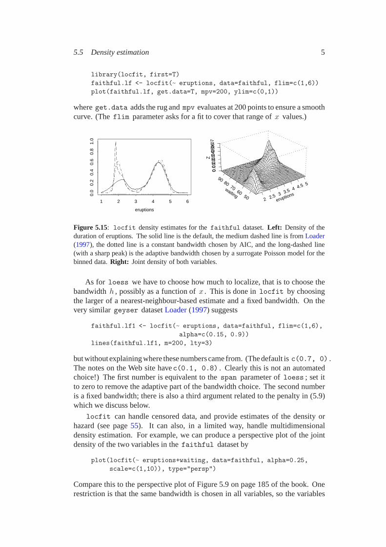
library(locfit, first=T)faithful.lf <- locfit(~ eruptions, data=faithful, flim=c(1,6))plot(faithful.lf, get.data=T, mpv=200, ylim=c(0,1))
where get.data adds the rug and mpv evaluates at 200 points to ensure a smoothcurve. (The flim parameter asks for a fit to cover that range of x values.)
eruptions
1 2 3 4 5 6
0.0
0.2
0.4
0.6
0.8
1.0
2 2.5 3 3.5 4 4.5 5
eruptions5060
7080
90
waiting
00.0
10.020.
030.0
40.05 0
.060.07
Z
Figure 5.15: locfit density estimates for the faithful dataset. Left: Density of theduration of eruptions. The solid line is the default, the medium dashed line is from Loader(1997), the dotted line is a constant bandwidth chosen by AIC, and the long-dashed line(with a sharp peak) is the adaptive bandwidth chosen by a surrogate Poisson model for thebinned data. Right: Joint density of both variables.
As for loess we have to choose how much to localize, that is to choose thebandwidth h , possibly as a function of x . This is done in locfit by choosingthe larger of a nearest-neighbour-based estimate and a fixed bandwidth. On thevery similar geyser dataset Loader (1997) suggests
faithful.lf1 <- locfit(~ eruptions, data=faithful, flim=c(1,6),alpha=c(0.15, 0.9))
lines(faithful.lf1, m=200, lty=3)
but without explaining where these numbers came from. (The default is c(0.7, 0) .The notes on the Web site havec(0.1, 0.8) . Clearly this is not an automatedchoice!) The first number is equivalent to the span parameter of loess ; set itto zero to remove the adaptive part of the bandwidth choice. The second numberis a fixed bandwidth; there is also a third argument related to the penalty in (5.9)which we discuss below.
locfit can handle censored data, and provide estimates of the density orhazard (see page 55). It can also, in a limited way, handle multidimensionaldensity estimation. For example, we can produce a perspective plot of the jointdensity of the two variables in the faithful dataset by
plot(locfit(~ eruptions+waiting, data=faithful, alpha=0.25,scale=c(1,10)), type="persp")
Compare this to the perspective plot of Figure 5.9 on page 185 of the book. Onerestriction is that the same bandwidth is chosen in all variables, so the variables

5.5 Density estimation 6
need to be rescaled6 to a scale on which such a bandwidth would be acceptable.(Setting scale=0 forces such a scale to be chosen.) The default is to use aspherically symmetric kernel, but kt="prod" chooses a product kernel.
Bandwidth selection
Loader advocates a local version of AIC for bandwidth selection. For a constantbandwidth he gives a function akaike . We use this for a gaussian kernel withstandard deviation h ∈ (0.1, 0.6) , remembering that density has 4 times andlocfit 2.5 times the standard error as the ‘bandwidth’ for a Gaussian kernel.
akaike <- function(formula, alpha, pen=2, ...){
m <- nrow(alpha); ll <- numeric(m); vr <- numeric(m)for(i in 1:m) {fit <- locfit(formula, alpha=alpha[i,], ...)ll[i] <- fit$dp["lk"]; vr[i] <- fit$dp["t0"]
}cbind(alpha=alpha, LogLik=ll, df=vr, AIC=-2*ll+pen*vr)
}attach(faithful)akaike( ~ eruptions,
alpha = cbind(0, 2.5 * seq( 0.1, 0.6, by = 0.05)),ev = "data", kern = "gauss")
LogLik df AIC[1,] 0 0.250 -249.8242 21.410054 542.4684[2,] 0 0.375 -255.1024 14.860509 539.9258[3,] 0 0.500 -258.1887 11.261502 538.9003[4,] 0 0.625 -259.1892 9.056460 536.4914[5,] 0 0.750 -258.8195 7.655461 532.9498[6,] 0 0.875 -257.7784 6.704812 528.9664[7,] 0 1.000 -256.5723 6.015671 525.1760[8,] 0 1.125 -255.8101 5.493791 522.6078[9,] 0 1.250 -256.2696 5.088088 522.7155
[10,] 0 1.375 -258.7174 4.764574 526.9640[11,] 0 1.500 -263.6509 4.497959 536.2977
The df term is the local version of the number of parameters. This suggestsh ≈ 0.48 , which we can fit by
fit <- locfit(~ eruptions, alpha = c(0, 1.2), flim = c(1, 6),kern = "gauss", ev = "grid", mg = 200)
lines(fit, m=200, lty=2)
The parameter ev controls where the fitted density is evaluated (and interpolationfrom these points is used for prediction). To find the AIC we evaluate at the datapoints, whereas for plotting we evaluate at a grid of mg points. The m argument oflines.locfit is equivalent to mpv , controlling the number of points at whichthe curve is plotted.
6 without this the computational shortcuts used by locfit fail in this example

5.5 Density estimation 7
Loader (1995) suggests an alternative approach, which is to bin the data andtreat the counts as independent Poisson variates (which they are not, but as forsurrogate Poisson GLMs this gives the correct likelihood). We can then use alocal log-linear model to smooth the counts, and allow its bandwidth to be chosenlocally by minimizing the local AIC.
erupt.bin <- data.frame(duration=seq(1.6, 5.1, by=0.05),count=hist(eruptions, breaks=seq(1.575, 5.125, by=0.05),
plot=F)$counts)fit2 <- locfit(count ~ duration, data=erupt.bin,
weights=rep(272*0.05, 71),alpha=c(0, 0, 2), family="poisson")
lines(fit2, m=200, lty=4)
This seems to be the most successful approach.
We can also consider the galaxies data.
plot(locfit(~ galaxies, flim=c(8000, 35000)),get.data=T, ylim=c(0, 0.0003), mpv=200)
akaike( ~ galaxies,alpha=cbind(seq( 0.15, 0.7, 0.05), 0),ev="data", kern="gauss")
[1,] 0.15 0 -763.8799 22.344750 1572.449[2,] 0.20 0 -769.8116 17.432047 1574.487[3,] 0.25 0 -772.8257 14.899450 1575.450[4,] 0.30 0 -773.0860 13.101204 1572.374[5,] 0.35 0 -773.8923 11.804248 1571.393[6,] 0.40 0 -774.1579 10.487591 1569.291[7,] 0.45 0 -774.7961 9.467591 1568.527[8,] 0.50 0 -776.1849 8.304028 1568.978[9,] 0.55 0 -776.7574 7.741446 1568.998
[10,] 0.60 0 -778.5080 7.316588 1571.649[11,] 0.65 0 -779.3692 6.922880 1572.584[12,] 0.70 0 -780.3391 6.610473 1573.899
fit <- locfit(~ galaxies, alpha=0.45, flim=c(8000, 35000),kern="gauss", ev="grid", mg=200)
lines(fit, m=200, lty=2)
galaxies.bin <- data.frame(velocity=seq(8000, 35000, 500),count=hist(galaxies, breaks=seq(7750, 35250, 500),
plot=F)$counts)fit2 <- locfit(count ~ velocity, data=galaxies.bin,
weights=rep(82*500, nrow(galaxies.bin)),alpha=c(0, 0, 2), family="poisson")
lines(fit2, m=200, lty=3)
Here the choice by local AIC of an adaptive bandwidth fails to work well, andseems very sensitive to the rounding used.
5.6 Bootstrap and permutation methods 8
galaxies
dens
ity
10000 15000 20000 25000 30000 35000
0.0
0.00
005
0.00
010
0.00
015
0.00
020
0.00
025
0.00
030
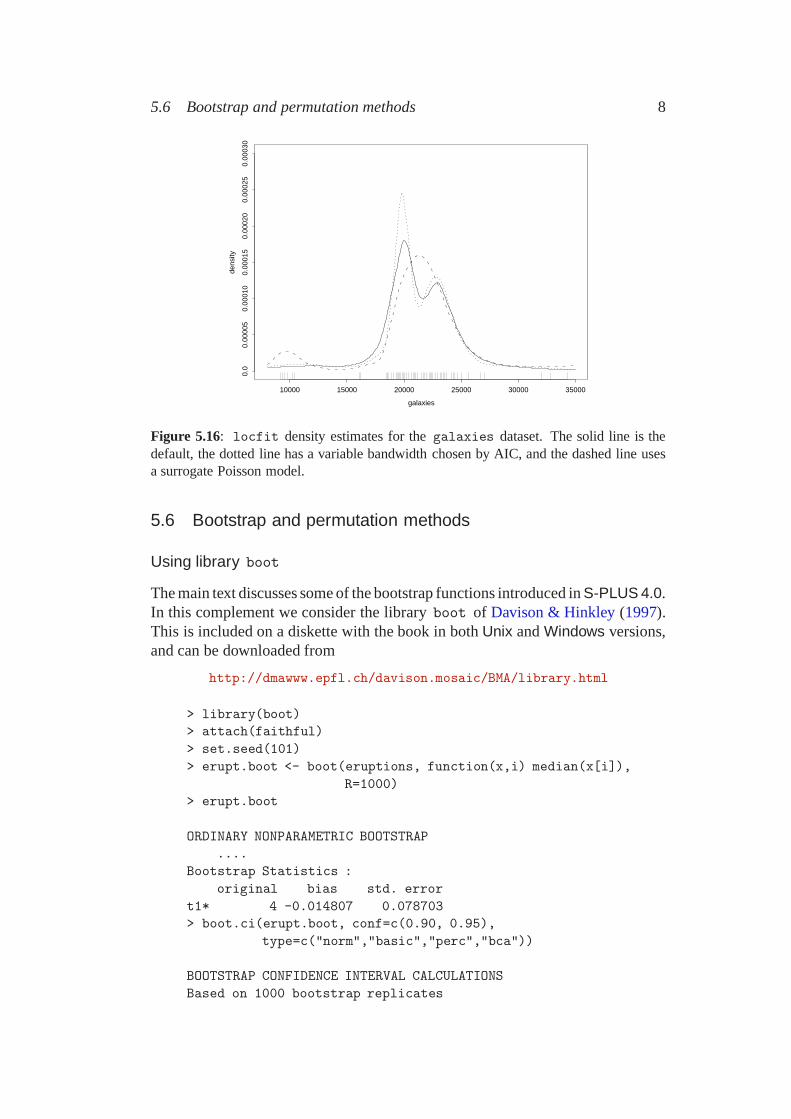
Figure 5.16: locfit density estimates for the galaxies dataset. The solid line is thedefault, the dotted line has a variable bandwidth chosen by AIC, and the dashed line usesa surrogate Poisson model.
5.6 Bootstrap and permutation methods
Using library boot
The main text discusses some of the bootstrap functions introduced in S-PLUS 4.0.In this complement we consider the library boot of Davison & Hinkley (1997).This is included on a diskette with the book in both Unix and Windows versions,and can be downloaded from
http://dmawww.epfl.ch/davison.mosaic/BMA/library.html
> library(boot)> attach(faithful)> set.seed(101)> erupt.boot <- boot(eruptions, function(x,i) median(x[i]),
R=1000)> erupt.boot
ORDINARY NONPARAMETRIC BOOTSTRAP....
Bootstrap Statistics :original bias std. error
t1* 4 -0.014807 0.078703> boot.ci(erupt.boot, conf=c(0.90, 0.95),
type=c("norm","basic","perc","bca"))
BOOTSTRAP CONFIDENCE INTERVAL CALCULATIONSBased on 1000 bootstrap replicates

5.6 Bootstrap and permutation methods 9
Intervals :Level Normal Basic90% ( 3.885, 4.144 ) ( 3.908, 4.167 )95% ( 3.861, 4.169 ) ( 3.892, 4.167 )
Level Percentile BCa90% ( 3.833, 4.092 ) ( 3.825, 4.083 )95% ( 3.833, 4.108 ) ( 3.759, 4.083 )Calculations and Intervals on Original ScaleSome BCa intervals may be unstable
Note that the results are similar to those using bootstrap , but not identical asthe random numbers are used in a different way. In this particular example theBCa confidence intervals are very slow to calculate.
Davison & Hinkley’s function boot is much more general than bootstrapin that it allows many other types of bootstrap sampling. What is commonlyknown as the bootstrap (random sampling with replacement from the originaldataset) is the default but boot can also perform a parametric bootstrap (sam-pling from a fitted distribution specified by argument ran.gen ), and stratified,weighted, balanced, antithetic and permutational sampling. Functions censbootand tsboot implement various forms of the bootstrap that have been suggestedfor right-censored data and time series respectively.
The function boot.ci calculates confidence intervals of one or more offive types, the first-order normal approximation, the percentile bootstrap interval(that found from the percentiles of the bootstrap distribution), the basic bootstrapinterval (the percentile interval reflected about the estimate) and the BCa correctionto the basic interval. Finally, it can calculate a studentized bootstrap interval (abasic bootstrap interval applied to a studentized statistic), and compute intervalson a transformed scale.
We also consider bootstrapping residuals from a non-linear regression onpp. 281–2. We can repeat that analysis with library boot by a very small changeto the function storm.bf . The bootstrapping here took about 90 seconds, theconfidence interval calculations about 5 seconds each. (The times for bootstrapunder 4.x are very similar.)
> storm.fm <- nls(Time ~ b*Viscosity/(Wt - c), stormer,start = c(b=29.401, c=2.2183))
> storm.bf <- function(rs, ind) {assign("Tim", fitted(storm.fm) + rs[ind], frame = 1)nls(Tim ~ (b * Viscosity)/(Wt - c), stormer,
start = coef(storm.fm))$parameters}
> rs <- scale(resid(storm.fm), scale = F)> storm.boot <- boot(rs, storm.bf, R = 1000)> storm.boot
....Bootstrap Statistics :
original bias std. error

5.6 Bootstrap and permutation methods 10
t1* 28.7156 0.71178 0.84350t2* 2.4799 -0.29007 0.60765
> boot.ci(storm.boot, index=1,type=c("norm", "basic", "perc", "bca"))
....Intervals :Level Normal Basic95% (26.35, 29.66 ) (26.29, 29.63 )Level Percentile BCa95% (27.80, 31.14 ) (27.10, 29.66 )Calculations and Intervals on Original ScaleWarning : BCa Intervals used Extreme QuantilesSome BCa intervals may be unstable
> boot.ci(storm.boot, index=2,type=c("norm", "basic", "perc", "bca"))
....Intervals :Level Normal Basic95% ( 1.579, 3.961 ) ( 1.632, 4.111 )Level Percentile BCa95% ( 0.848, 3.328 ) ( 1.588, 3.802 )Calculations and Intervals on Original ScaleSome BCa intervals may be unstable
The index parameter selects which of the components of the statistic are ofinterest. In this example it looks as if the percentile interval has a considerablebias. For reference, BCa intervals from the bootstrap output are given inSection 9.4 of these complements.
Using library bootstra
Another, older, set of bootstrap functions written by Rob Tibshirani accompaniesEfron & Tibshirani (1993). This is usually installed as library section bootstrapon a Unix machine but as bootstra on a Windows machine7. This too has afunction bootstrap to perform the bootstrap sampling, and other functions tofind bootstrap confidence intervals which similar code to bootstrap internally.This S code is written less efficiently than that in 4.x or boot , and should be usedwith care to avoid using excessive amounts of memory.
There is little advantage in using this function bootstrap for simple bootstrapsampling, as there are no special tools to analyse its results.
> library(bootstra)> attach(faithful)> set.seed(101)> erupt.boot <- bootstrap(eruptions, 1000, median)
7 since S-PLUS 3.x for Windows can only use MSDOS 8+3 filenames.

5.6 Bootstrap and permutation methods 11
> mean(erupt.boot$thetastar - median(eruptions))[1] -0.014807> sqrt(var(erupt.boot$thetastar))[1] 0.078703
However, the function bootstrap also incorporates the ‘jackknife after boot-strap’ technique.
set.seed(101)erupt.boot2 <- bootstrap(eruptions, 1000, median, func=mean)At least one jackknife influence value for func(theta) is
undefinedIncrease nboot and try again
As this code was already using 25 Mb of memory, this is not practicable advice.This library has functions bcanon and boott to compute BCa and studen-
tized confidence limits, but the first fails on this example.
set.seed(101)boott(eruptions, median, perc=c(0.025, 0.05, 0.95, 0.975))$confpoints:
0.025 0.05 0.95 0.975[1,] 3.7925 3.8485 4.1219 4.1351
We can also consider the Stormer viscometer data from Section 9.4. Therewe bootstrap residuals, so cannot use the jackknife directly and hence bcanon(which tries to evaluate the function on vectors of size n − 1 ) fails. We can useboott , but it is slow (15 minutes), especially so as the bootstrapping has to berun separately for each component of the parameter.
storm.bf1 <- function(rs) {assign("Tim", fitted(storm.fm) + rs, frame = 1)nls(Tim ~ (b * Viscosity)/(Wt - c), stormer,
start = coef(storm.fm))$parameters[1]}
storm.bf2 <- function(rs) {assign("Tim", fitted(storm.fm) + rs, frame = 1)nls(Tim ~ (b * Viscosity)/(Wt - c), stormer,
start = coef(storm.fm))$parameters[2]}
set.seed(101)boott(rs, storm.bf1, perc=c(0.025, 0.05, 0.95, 0.975))$confpoints:
0.025 0.05 0.95 0.975[1,] 26.434 26.825 29.228 29.336set.seed(101)boott(rs, storm.bf2, perc=c(0.025, 0.05, 0.95, 0.975))$confpoints:
0.025 0.05 0.95 0.975[1,] 1.8939 2.0168 3.6694 3.8459

12
Chapter 7
Generalized Linear Models
7.1 Functions for generalized linear modelling
Estimation of the dispersion parameter ϕ
We saw on page 226 that an approximately unbiased estimator of the dispersionparameter ϕ is
ϕ =DM
n− p
This is not, however, the estimator used by summary.glm , which is the sum ofsquares of the Pearson residuals divided by the residual degrees of freedom. Thus
ϕ =1
n− p
∑i
(yi − µi)2
V (µi)/Ai(7.11)
where V (µ) is the variance function. (Here p is the number of linearly inde-pendent parameters.) Note that ϕ = ϕ for the Gaussian family, but in generaldiffers.
The estimate of dispersion is only used to compute the estimated standard er-rors of the coefficients, and only for the binomial and Poisson families if summaryis called with argument dispersion=0 . We explore further the estimation of thedispersion parameter for a Gamma family in Section 7.5.
7.3 Poisson models
Log-linear models with formulae and data frames
The standard function loglin fits a log-linear model to frequency data by iter-ative proportional scaling, which can be more computationally efficient than thesurrogate Poisson model approach, particularly for very large frequency arrays.However, it has several limitations.

7.3 Poisson models 13
• It can only handle categorical predictor variables, and the frequencies mustbe given as a complete multiway frequency table. Missing cells (or structuralzeros) can be handled. Note that this is not a necessary restriction; the moregeneral algorithm developed in Darroch & Ratcliff (1972) can handle bothquantitative and categorical predictors.
• It cannot discover redundancies in the underlying model matrix. Hence ifthere are missing cells loglin may report an incorrect number of error de-grees of freedom. This restriction is difficult to overcome without explicitlyconstructing the model matrix, something that iterative proportional scalingalgorithms are designed to avoid.
• Deviances and fitted values are the main products of the algorithm. If theinput frequency array has no missing cells and none with zero fitted values,constrained parameter estimates relative to a complete dummy variablemodel matrix are available, but their standard errors are not.
Nevertheless it is an important and useful fitting algorithm for very large frequencytables.
The algorithm is based on the score equations for Poisson data with the naturallog link. That is, the mean vector, µ , must have the appropriate multiplicativestructure and satisfy
XT y = XT µ
where X is the model matrix. With purely categorical predictors this implies thatthe arrays of observed frequencies and of the fitted values have identical marginaltotals. Hence it is sufficient to specify the margins over which frequency and fittedvalues must have the same totals. For example, for a three-way frequency table,Fr , the ‘no three-factor-interaction’ model may be specified by
loglin(Fr, list(c(1,2), c(1,3), c(2,3)))
where the second argument specifies that all two-way faces must have the samemarginal totals. If Fr has a dimnames attribute with named components themarginal faces may be specified using these names, so if we set
names(dimnames(Fr)) <- c("A", "B", "C")
we could specify the no three-factor-interaction model as
loglin(Fr, list(c("A","B"), c("A","C"), c("B","C")))
Note that if the c(1,2) -face is specified then all faces marginal to it—the firstand second dimensions and the entire array—also have equal frequency and fittedvalue totals. These redundant faces may also be specified, although this may slowdown the algorithm slightly.
The function loglm in the MASS library is designed to make calls to loglineasier by allowing the fixed margins to be specified by an S formula and thefrequencies to be specified either as an array or as a vector in, for example, a dataframe. In the latter case the frequency array will be constructed before calling

7.3 Poisson models 14
loglin . If the frequencies are specified as an array, the formula has an emptyleft-hand side and the right-hand side specifies the fixed marginal totals. Thus theprevious example could be handled by calling either
loglm(~ (1 + 2 + 3)^2, Fr)
or, if the dimnames are present,
loglm(~ (A + B + C)^2, Fr)
Note that the dimensions of the array may always be referred to by number usingthe same convention as loglin , and that any multiplicative-like term connectingthe faces, such as 1:2 , 1*2 or even 1/2 , simply implies ‘the c(1,2) -face’. Inconstructing the call to loglin , loglm finds and uses only the minimal set ofmarginal totals which must agree, so it does not matter if (as here) the formulaspecifies some redundant margins.
Let us consider the detergent brand preference study on page 238–242 ofChapter 7, which is a four-way contingency table. We can fit the final modelspecified as a GLM on page 240 using the same formula in a call to loglm .
> detg.ll <- loglm(Fr ~ Brand*M.user*Temp + M.user*Temp*Soft,data=detg)
> detg.ll....
Statistics:X^2 df P(> X^2)
Likelihood Ratio 5.6561 8 0.68570Pearson 5.6500 8 0.68637
This call to loglm actually constructs the iterative proportional scaling fit vialoglin shown as detg.ips on page 241.
For another example, consider the Minnesota school leavers’ data of 1938.The frequencies are held in the data frame minn38 , but this is easily convertedinto a complete frequency array.
> sapply(minn38, function(x) length(levels(x)))hs phs fol sex f3 4 7 2 0
> minn38a <- array(0, c(3,4,7,2), lapply(minn38[, -5], levels))> minn38a[data.matrix(minn38[, -5])] <- minn38$f> minn38.fm <- loglm(~ 1 + 2 + 3 + 4, minn38a)> minn38.fm1 <- update(minn38.fm, ~.^2)> minn38.fm2 <- update(minn38.fm, ~.^3)
This uses numeric labels for the variables (dimensions) and fits complete 1–, 2–and 3–factor interaction models. Since this way of constructing the array alsosupplies names for the dimnames attribute, we could have specified the firstmodel as
minn38.fm <- loglm(~ hs + phs + fol + sex, minn38a)

7.3 Poisson models 15
and subsequent updates would have carried the names forward. The advantagewould have that later output will carry the informative names rather than thenumeric labels. The object resulting from a call to loglm carries class loglm ,for which methods for the generic functions summary , print , anova , coef ,deviance , fitted , residuals and update are provided.
The print method displays the object in a succinct way.
> minn38.fm....
Statistics:X^2 df P(> X^2)
Likelihood Ratio 3711.9 155 0Pearson 4161.6 155 0
The default behaviour for the summary method is to give almost the sameoutput, but with the argument fitted=T this will also give tables of observedand expected frequencies. For example
> summary(minn38.fm2, fitted=T)Re-fitting to find fitted valuesFormula:~ 1 + 2 + 3 + 4 + 1:2 + 1:3 + 1:4 + 2:3 + 2:4 + 3:4 +
1:2:3 + 1:2:4 + 1:3:4 + 2:3:4
Statistics:X^2 df P(> X^2)
Likelihood Ratio 47.745 36 0.091137Pearson 47.184 36 0.100486
Observed (Expected):
, , F1, FC E N O
L 53 ( 49.5) 13 ( 16.6) 7 ( 7.6) 76 ( 75.4)M 163 (163.6) 28 ( 25.8) 30 ( 29.1) 118 (120.5)U 309 (311.9) 38 ( 36.6) 17 ( 17.3) 89 ( 87.2)
, , F2, FC E N O
L 36 ( 31.5) 11 ( 13.9) 16 ( 13.2) 111 (115.4)M 116 (112.8) 53 ( 47.8) 41 ( 42.6) 214 (220.8)U 225 (232.7) 68 ( 70.3) 49 ( 50.2) 210 (198.8)
....
The model will be re-fitted unless fit=T was specified on the original call tologlm .
We can compare the models by likelihood-ratio tests using
> anova(minn38.fm, minn38.fm1, minn38.fm2)LR tests for hierarchical log-linear models

7.3 Poisson models 16
Model 1:~ 1 + 2 + 3 + 4
Model 2:~ 1 + 2 + 3 + 4 + 1:2 + 1:3 + 1:4 + 2:3 + 2:4 + 3:4
Model 3:~ 1 + 2 + 3 + 4 + 1:2 + 1:3 + 1:4 + 2:3 + 2:4 + 3:4
+ 1:2:3 + 1:2:4 + 1:3:4 + 2:3:4Deviance df Delta(Dev) Delta(df) P(> Delta(Dev))
Model 1 3711.915 155Model 2 220.043 108 3491.873 47 0.00000Model 3 47.745 36 172.298 72 0.00000
Saturated 0.000 0 47.745 36 0.09114
The tail areas refer to the approximate chi-squared distribution under the nullhypothesis. In this instance only the final model appears near reasonable as adescription of the data.
The function loglm is generic with method dispatch based on the secondargument (data ) rather than the first. It has a method for objects of classcrosstabs which is the natural way of tabulating frequencies, particularly forfactors held in data frames. For example the Cars93 data frame has informationon 93 models of car released in the USA in 1993. Two factors are Type andOrigin .
> attach(Cars93)> levels(Type)[1] "Compact" "Large" "Midsize" "Small" "Sporty" "Van"> levels(Origin)[1] "Import" "Local"> detach()
We could check the (unlikely) hypothesis that the proportions of each type ofvehicle are the same for imported and locally manufactured cars using
> form <- ~ Type + Origin> loglm(form, crosstabs(form, Cars93))
....Statistics:
X^2 df P(> X^2)Likelihood Ratio 18.362 5 0.0025255
Pearson 14.080 5 0.0151101
The Minnesota school leavers’ example could be handled without explicitlyconstructing the array of frequencies by the call
minn38.fm <- loglm(f ~ ., minn38, fit = T)
Note that arguments to loglin may be specified on the call to loglm . The extraargument, fit=T , is not needed here but if supplied will cause the fitted values(and by default the frequencies as well) to be saved as an array in the fitted modelobject. Note that the customary abbreviation, ‘. ’, may be used to specify ‘all

7.3 Poisson models 17
other factors in the data frame joined by + ’. (This is not possible if the data aregiven as an array of frequencies.)
The Quine absenteeism data is an example of a four-way classification withunequal numbers of observations in each cell including some completely empty.The maximum number of observations in any one cell is 11. In cases like this thefrequencies will be held as a five-way array with the last dimension, conventionallylabelled .Within. , playing no part in the fitted models. Empty cells in the five-way array are handled as structural zeros. The result will be a fitted log-linearmodel with correct deviance, but with residual degrees of freedom is sometimesincorrect.
> quine.loglm <- loglm(Days ~ .^3, quine)> quine.glm <- glm(Days ~ .^3, poisson, quine)> c(loglm = deviance(quine.loglm), glm = deviance(quine.glm))loglm glm1181 1181
> c(loglm = quine.loglm$df, glm = quine.glm$df)loglm glm117 120
Notice that (unlike loglin ) loglm does subtract one degree of freedom forstructural zeros, but is unable to detect the extra three degrees of freedom thatresult from redundancies in the model matrix.
How loglm works
The function loglm must be able to convert numeric labels in formulae to a form inwhich they can be parsed correctly. This operation is done by a recursive functioncalled denumerate which converts a numeric label 2 , say, to the identifier .v2 .
> denumeratefunction(object) UseMethod("denumerate")> denumerate.formulafunction(x){
if(length(x) == 1) {if(mode(x) == "numeric" || (mode(x) == "name" &&any(substring(x, 1, 1) == as.character(1:9))))x <- as.name(paste(".v", x, sep = ""))
}else {x[[2]] <- Recall(x[[2]])if(length(x) == 3 && x[[1]] != as.name("^"))x[[3]] <- Recall(x[[3]])
}x
}

7.5 Gamma models 18
It is not intended to be called directly by the user, but if it is, unless the object givento it is a formula it will issue a (somewhat cryptic) error message. This is oneintended side-effect of making the function generic. The function renumerateis similar and converts the encoded identifiers to numeric labels. These functionsprovide examples of how operations on the language itself are possible and notparticularly difficult.
7.5 Gamma models
The role of dispersion parameter ϕ in the theory and practice of GLMs is oftenconfusing (and not just in notation as pointed out on page 226). For a Gaussianfamily with identity link the moment estimator used for ϕ is the usually unbiasedmodification of the maximum likelihood estimator (see equations (7.6) and (7.7)).For binomial and Poisson families we usually take ϕ = 1 , and when we allow ϕto vary it is almost always as an ad hoc adjustment for over-dispersion which doesnot correspond precisely to any family of error distributions. (Of course, for thePoisson family the negative binomial family introduced in Section 7.4 provides aparametric alternative way of modelling over-dispersion.)
The situation for the Gamma family is rather different. This is a parametricfamily which can be fitted by maximum likelihood, including its shape parameterα . Elsewhere we have taken its density as
log f(y) = α log λ+ (α− 1) log y − λy − log Γ(α)
so the mean is µ = α/λ . If we re-parametrize by (µ, α) we obtain
log f(y) = α(−y/µ − log µ) + α log y + α logα − log y − log Γ(α)
Comparing this with the general form in equation (7.1) (on page 223) we seethat the canonical link is θ = 1/µ and ϕ = 1/α is the dispersion parameter.For fixed ϕ , fitting by glm gives the maximum likelihood estimates of theparameters in the linear predictor, but ϕ is estimated from the sum of squaresof the deviance residuals, which need not be similar to the maximum likelihoodestimator. Note that ϕ is used to estimate the standard errors for the parameters inthe linear predictor, so appreciable differences in the estimate can have practicalsignificance.
Some authors (notably McCullagh & Nelder (1989, pp. 295–6)) have arguedagainst the maximum likelihood estimator of ϕ . The MLE is the solution to
2n [logα − ψ(α)] = D
where ψ = Γ′/Γ is the digamma function and D is the residual deviance. Thenthe customary estimator of ϕ = 1/α is D/(n−p) and the MLE is approximately1
1 for large α

7.5 Gamma models 19
D(6 + D)/(6 + 2D) where D = D/n . Both the customary estimator (7.7) andthe MLE are based on the residual deviance
D = −2∑
i
[log(yi/µi) − (yi − µi)/µi]
and this is very sensitive to small values of yi . Another argument is that if thegamma GLM is being used as a model for distributions with a constant coefficientof variation, the MLE is inconsistent for the true coefficient of variation exceptat the gamma family. These arguments are equally compelling for the customaryestimate; McCullagh & Nelder prefer the moment estimator
σ2 = 1n−p
∑[(yi − µi)/µi]
2 (7.12)
for the coefficient of variation σ2 which equals ϕ under the gamma model. Thiscoincides with ϕ as quoted by summary.glm (see (7.11) on page 12).
The functions glm.shape and glm.dispersion in library MASS computethe MLEs of α and ϕ respectively from a fitted Gamma glm object. We illustratethese with an example on clotting times of blood taken from McCullagh & Nelder(1989, pp. 300–2).
> clotting <- data.frame(u = c(5,10,15,20,30,40,60,80,100),lot1 = c(118,58,42,35,27,25,21,19,18),lot2 = c(69,35,26,21,18,16,13,12,12) )
> clot1 <- glm(lot1 ~ log(u), data=clotting, family=Gamma)> summary(clot1, cor=F)Coefficients:
Value Std. Error t value(Intercept) -0.016554 0.00092754 -17.848
log(u) 0.015343 0.00041496 36.975
(Dispersion Parameter for Gamma family taken to be 0.00245 )
> clot1$deviance/clot1$df.residual[1] 0.00239> gamma.dispersion(clot1)[1] 0.0018583
> clot2 <- glm(lot2 ~ log(u), data=clotting, family=Gamma)> summary(clot2, cor=F)Coefficients:
Value Std. Error t value(Intercept) -0.023908 0.00132645 -18.024
log(u) 0.023599 0.00057678 40.915
(Dispersion Parameter for Gamma family taken to be 0.00181 )
> clot2$deviance/clot2$df.residual

7.5 Gamma models 20
[1] 0.0018103> gamma.dispersion(clot2)[1] 0.0014076
The differences here are enough to affect the standard errors, but the shape pa-rameter of the gamma distribution is so large that we have effectively a normaldistribution with constant coefficient of variation.
These functions may also be used for a quasi family with variance propor-tional to mean squared. We illustrate this on the quine dataset.
> gm <- glm(Days + 0.1 ~ Age*Eth*Sex*Lrn,quasi(link=log, variance=mu^2), data=quine)
> summary(gm, cor=F)Coefficients: (4 not defined because of singularities)
Value Std. Error t valueValue Std. Error t value
(Intercept) 3.06105 0.39152 7.818410AgeF1 -0.61870 0.52528 -1.177863AgeF2 -2.31911 0.87546 -2.649018AgeF3 -0.37623 0.47055 -0.799564
....
(Dispersion Parameter for Quasi-likelihood family takento be 0.61315 )
Null Deviance: 190.4 on 145 degrees of freedomResidual Deviance: 128.36 on 118 degrees of freedom
> gamma.shape(gm, verbose=T)Initial estimate: 1.0603Iter. 1 Alpha: 1.23840774338543Iter. 2 Alpha: 1.27699745778205Iter. 3 Alpha: 1.27834332265501Iter. 4 Alpha: 1.27834485787226
Alpha: 1.27834SE: 0.13452
> summary(gm, dispersion = gamma.dispersion(gm), cor=F)Coefficients: (4 not defined because of singularities)
Value Std. Error t value(Intercept) 3.06105 0.44223 6.921890
AgeF1 -0.61870 0.59331 -1.042800AgeF2 -2.31911 0.98885 -2.345261AgeF3 -0.37623 0.53149 -0.707880
....
In this example the McCullagh–Nelder preferred estimate is given by
> sum((residuals(gm, type="resp")/fitted(gm))^2/gm$df.residual)[1] 0.61347

7.5 Gamma models 21
which is the same as the estimate returned by summary.glm , whereas (7.7) gives
> gm$deviance/gm$df.residual[1] 1.0878> gamma.dispersion(gm)[1] 0.78226
There will also be differences between deviance tests and the AIC used bystep.glm and likelihood-ratio tests and the exact AIC. Making the necessarymodifications is left as an exercise for the reader.

22
Chapter 9
Non-linear Models
9.4 Confidence intervals for parameters
Bootstrapping
In this example the empirical percentile intervals appear biased, especially thatfor c . Running a different simulation gives
> storm.boot <- bootstrap(rs, storm.bf, seed=101, B=1000)> summary(storm.boot)
....Summary Statistics:
Observed Bias Mean SEb 28.72 0.6821 29.398 0.8304c 2.48 -0.2506 2.229 0.6090
Empirical Percentiles:2.5% 5% 95% 97.5%
b 27.6406 27.989 30.734 30.91c 0.9906 1.238 3.224 3.43
BCa Percentiles:2.5% 5% 95% 97.5%
b 26.616 26.661 29.433 29.681c 1.532 1.724 3.618 3.958
Correlation of Replicates:b c
b 1.0000 -0.9193c -0.9193 1.0000
Note that there will be warnings that indicate that the use of jackknifing in thisproblem is unreliable, so the BCa intervals are not to be trusted.
A ‘jackknife after bootstrap’ analysis confirms that the bootstrap estimates ofthe bias in the least-squares estimates is indicative but not statistically significant.

9.4 Confidence intervals for parameters 23
> jack.after.bootstrap(storm.boot, "Bias")....
Functional of Bootstrap Distribution of Parameters:Func SE.Func
b 0.6821 0.5084c -0.2506 0.2168
Observations with Large Influence on Functional:$b:
b6 -2.371
An alternative approach using the library boot of Davison & Hinkley (1997)is given in Section 5.6 of these Complements.

24
Chapter 10
Random and Mixed Effects
The account in the text used version 2.1 of the nlme software contained inS-PLUS 3.4, 4.0, 4.5 and 5.0. A near-final release of version 3.0 (written byPinheiro and Bates) is now available from
http://nlme.stat.wisc.edu
for both Unix and Windows versions of S-PLUS 3.x and 4.x, and it is planned thatthis will be incorporated into forthcoming releases of S-PLUS. In this chapter wediscuss the changes need to make our examples work with version 3.0, and alsoexplore some analyses which were not straightforward in earlier versions.
The main innovation in nlme version 3.0 is support of multilevel randomeffects; however much of the system has been rewritten and the user interfacere-designed. The new system needs to override the old one, so use
library(nlme3, first=T) # or whatever name is used locally
if the library has been downloaded and added.
10.3 Linear mixed effects models
The main change is how the ‘clusters’ are specified, which now has to allowmultilevel random effects and is usually done by conditioning the formula in therandom argument in a very similar way to Trellis formulae.
The method of estimation (REML or maximum likelihood) is specified by theargument method rather than est.method .
Making these changes to the gasoline data petrol example gives
> Petrol <- petrol> Petrol[, 2:5] <- scale(as.matrix(Petrol[, 2:5]), scale = F)> pet3.lme <- lme(Y ~ SG + VP + V10 + EP,
random = ~ 1 | No, data = Petrol)> summary(pet3.lme)Linear mixed-effects model fit by REMLData: Petrol
AIC BIC logLik

10.3 Linear mixed effects models 25
166.38 175.45 -76.191
Random effects:Formula: ~ 1 | No
(Intercept) ResidualStdDev: 1.4447 1.8722
Fixed effects: Y ~ SG + VP + V10 + EPValue Std.Error DF t-value p-value
(Intercept) 19.707 0.56827 21 34.679 <.0001SG 0.219 0.14694 6 1.493 0.1860VP 0.546 0.52052 6 1.049 0.3347V10 -0.154 0.03996 6 -3.860 0.0084EP 0.157 0.00559 21 28.128 <.0001
....
Note a change in value of BIC (which is no longer qualified as ‘restricted’) andthe changes in the printed output for the fixed effects.
> pet3.lme <- update(pet3.lme, method = "ML")> summary(pet3.lme)Linear mixed-effects model fit by maximum likelihoodData: Petrol
AIC BIC logLik149.38 159.64 -67.692
Random effects:Formula: ~ 1 | No
(Intercept) ResidualStdDev: 0.92889 1.8273
Fixed effects: Y ~ SG + VP + V10 + EPValue Std.Error DF t-value p-value
(Intercept) 19.694 0.47815 21 41.188 <.0001SG 0.221 0.12282 6 1.802 0.1216VP 0.549 0.44076 6 1.246 0.2590V10 -0.153 0.03417 6 -4.469 0.0042EP 0.156 0.00587 21 26.620 <.0001
....> pet4.lme <- update(pet3.lme, fixed = Y ~ V10 + EP)> anova(pet4.lme, pet3.lme)
Model df AIC BIC logLik Test Lik.Ratiopet4.lme 1 5 149.61 156.94 -69.806pet3.lme 2 7 149.38 159.64 -67.692 1 vs. 2 4.2285
p-valuepet4.lmepet3.lme 0.1207> coef(pet4.lme)
(Intercept) V10 EPA 21.054 -0.21081 0.15759

10.3 Linear mixed effects models 26
....> pet5.lme <- update(pet4.lme, random = ~ 1 + EP | No)> anova(pet4.lme, pet5.lme)
Model df AIC BIC logLik Test Lik.Ratiopet4.lme 1 5 149.61 156.94 -69.806pet5.lme 2 7 153.61 163.87 -69.805 1 vs. 2 0.0025194
p-valuepet4.lmepet5.lme 0.9987
It is possible to handle the oats example as in the text, but this is mostnaturally handled by making use of multilevel random effects.
> options(contrasts = c("contr.treatment", "contr.poly"))> oats.lme <- lme(Y ~ N + V, random = ~1 | B/V, data=oats)> summary(oats.lme)Data: oats
AIC BIC logLik586.07 605.78 -284.03
Random effects:Formula: ~ 1 | B
(Intercept)StdDev: 14.645
Formula: ~ 1 | V %in% B(Intercept) Residual
StdDev: 10.473 12.75
Fixed effects: Y ~ N + VValue Std.Error DF t-value p-value
(Intercept) 79.917 8.2203 51 9.722 <.0001N0.2cwt 19.500 4.2500 51 4.588 <.0001N0.4cwt 34.833 4.2500 51 8.196 <.0001N0.6cwt 44.000 4.2500 51 10.353 <.0001
VMarvellous 5.292 7.0789 10 0.748 0.4720VVictory -6.875 7.0789 10 -0.971 0.3544....
Number of Observations: 72Number of Groups:B V %in% B6 18
Notice that we specify multilevel random effects as a nested model in exactly thesame way as a Error term in a aov model.
The approach via specifying a covariance structure still works: two equivalentspecifications are given by
oats$sp <- model.matrix(~ V - 1, oats)oats1.lme <- lme(Y ~ N + V, oats,

10.3 Linear mixed effects models 27
random = list(B = pdBlocked(list(~1, pdIdent(~sp-1)))))summary(oats1.lme)oats2.lme <- lme(Y ~ N + V,
random = reStruct(~ V - 1 | B, "pdCompSymm"),data = oats)
summary(oats2.lme)
It should be clear that these are less than obvious, and we are grateful to DrPinheiro for elucidating the precise forms needed.
The multilevel approach allows us to handle easily the cooperative trial by
lme(Conc ~ 1, random = ~1 | Lab/Bat, data = coop,subset = Spc=="S1")
Linear mixed-effects model fit by REMLData: coopSubset: Spc == "S1"Log-restricted-likelihood: 21.022Fixed: Conc ~ 1
(Intercept)0.50806
Random effects:Formula: ~ 1 | Lab
(Intercept)StdDev: 0.24529
Formula: ~ 1 | Bat %in% Lab(Intercept) Residual
StdDev: 0.073267 0.079355
Number of Observations: 36Number of Groups:Lab Bat %in% Lab6 18
which agrees with the raov analysis.
Sitka spruce example
There is a problem with the analysis of this example in the text: we misunder-stood the meaning of the correlation model fitted which was in fact in units ofthe meaurement number, not days. We first consider an analysis without serialcorrelation.
> sitka.lme <- lme(size ~ treat*ordered(Time),random = ~1 | tree, data = Sitka)
> summary(sitka.lme)Linear mixed-effects model fit by REMLData: Sitka
AIC BIC logLik

10.3 Linear mixed effects models 28
79.901 127.34 -27.95
Random effects:Formula: ~ 1 | tree
(Intercept) ResidualStdDev: 0.61011 0.16105
Fixed effects: size ~ treat * ordered(Time)Value Std.Error DF t-value p-value
(Intercept) 4.9851 0.12287 308 40.572 <.0001treat -0.2112 0.14861 77 -1.421 0.1594
ordered(Time).L 1.1971 0.03221 308 37.166 <.0001ordered(Time).Q -0.1341 0.03221 308 -4.162 <.0001ordered(Time).C -0.0409 0.03221 308 -1.268 0.2056
ordered(Time) ^ 4 -0.0273 0.03221 308 -0.848 0.3974treatordered(Time).L -0.1786 0.03896 308 -4.583 <.0001treatordered(Time).Q -0.0264 0.03896 308 -0.679 0.4977treatordered(Time).C -0.0142 0.03896 308 -0.366 0.7148
treatordered(Time) ^ 4 0.0124 0.03896 308 0.318 0.7504....
> attach(Sitka)> Sitka$treatslope <- Time * (treat=="ozone")> detach()> sitka.lme2 <- update(sitka.lme,
fixed = size ~ ordered(Time) + treat + treatslope)> summary(sitka.lme2)Linear mixed-effects model fit by REMLData: Sitka
AIC BIC logLik69.269 104.92 -25.635
Random effects:Formula: ~ 1 | tree
(Intercept) ResidualStdDev: 0.61015 0.1604
Fixed effects: size ~ ordered(Time) + treat + treatslopeValue Std.Error DF t-value p-value
(Intercept) 4.9851 0.12287 311 40.572 <.0001ordered(Time).L 1.1976 0.03204 311 37.372 <.0001ordered(Time).Q -0.1455 0.01810 311 -8.037 <.0001ordered(Time).C -0.0506 0.01805 311 -2.804 0.0054
ordered(Time) ^ 4 -0.0167 0.01805 311 -0.926 0.3549treat 0.2217 0.17561 77 1.262 0.2107
treatslope -0.0021 0.00046 311 -4.626 <.0001....
Note that although the model is different, the conclusions are very similar.Predictions and fitted values are specified somewhat differently in the later
version of lme . The random effects are now specified by level, with the ‘popula-

10.3 Linear mixed effects models 29
tion’ values at level 0 and the BLUPs used up to the level specified (which defaultsto the innermost level). Thus we can examine the fitted mean values by
> fitted(sitka.lme2, level = 0)[1:5]1 1 1 1 1
4.0606 4.4709 4.8427 5.1789 5.3167> fitted(sitka.lme2, level = 0)[301:305]
61 61 61 61 614.164 4.6213 5.0509 5.4427 5.6467
The names tell us that these correspond to trees 1 and 61, but at level 0 are thesame for all the trees in a treatment group.
We can specify a correlation structure by
lme(size ~ treat*ordered(Time), random = ~1 | tree,data = Sitka, corr = corCAR1(, ~Time | tree))
but this will not converge properly (the reported correlation coefficient is 0.2 ,the default starting value). If we give it a better initial value it does converge:
> sitka.lme <-lme(size ~ treat*ordered(Time), random = ~1 | tree,
data = Sitka, corr = corCAR1(0.9, ~Time | tree))> summary(sitka.lme)Correlation Structure: Continuous AR(1)Parameter estimate(s):
Phi0.9989
Fixed effects: size ~ treat * ordered(Time)Value Std.Error DF t-value p-value
(Intercept) 4.9851 0.12636 308 39.452 <.0001treat -0.2112 0.15284 77 -1.382 0.1711
ordered(Time).L 1.1971 0.04907 308 24.396 <.0001ordered(Time).Q -0.1341 0.02642 308 -5.073 <.0001ordered(Time).C -0.0409 0.01979 308 -2.065 0.0398
ordered(Time) ^ 4 -0.0273 0.01673 308 -1.632 0.1037treatordered(Time).L -0.1786 0.05935 308 -3.009 0.0028treatordered(Time).Q -0.0264 0.03196 308 -0.827 0.4086treatordered(Time).C -0.0142 0.02394 308 -0.595 0.5521
treatordered(Time) ^ 4 0.0124 0.02023 308 0.613 0.5403
Note that the specification of the correlation structures has altered: see the helpon corClasses for the current form.
The specification of a systematic component to the variances1has also altered,now using the weights argument; see the help on varClasses .
1 mentioned on pages 310 and 312 but not used in our examples

10.4 Non-linear mixed effects models 30
10.4 Non-linear mixed effects models
The changes needed to use nlme are similar to those for lme : specify the‘clusters’ by conditioning the random effects formulae, use 1 rather than . is theformulae, and the method is specified by method , still defaulting to maximumlikelihood.
For the sitka data we first fit without a correlation structure.
> options(contrasts = c("contr.treatment", "contr.poly"))> sitka.nlme <- nlme(size ~ A + B * (1 - exp(-(Time-100)/C)),
fixed = list(A ~ treat, B ~ treat, C ~ 1),random = A + B ~ 1 | tree, data = Sitka,start = list(fixed = c(2, 0, 4, 0, 100)),method = "ML", verbose = T)
> summary(sitka.nlme)Nonlinear mixed-effects model fit by maximum likelihoodModel: size ~ A + B * (1 - exp( - (Time - 100)/C))
Data: SitkaAIC BIC logLik
-96.275 -60.465 57.138
Random effects:Formula: list(A ~ 1, B ~ 1)Level: treeStructure: General positive-definite
StdDev CorrA.(Intercept) 0.83561 A.(IntB.(Intercept) 0.81954 -0.69
Residual 0.10297
Fixed effects: list(A ~ treat, B ~ treat, C ~ 1)Value Std.Error DF t-value p-value
A.(Intercept) 2.304 0.1995 312 11.547 <.0001A.treat 0.175 0.2117 312 0.826 0.4096
B.(Intercept) 3.921 0.1808 312 21.687 <.0001B.treat -0.564 0.2156 312 -2.618 0.0093
C 81.769 4.7270 312 17.299 <.0001....
> sitka.nlme2 <- update(sitka.nlme,fixed = list(A ~ 1, B ~ 1, C ~ 1),start = list(fixed=c(2.3, 3.9, 79)))
> summary(sitka.nlme2)Nonlinear mixed-effects model fit by maximum likelihoodModel: size ~ A + B * (1 - exp( - (Time - 100)/C))
Data: SitkaAIC BIC logLik
-91.588 -63.736 52.794....

10.4 Non-linear mixed effects models 31
Fixed effects: list(A ~ 1, B ~ 1, C ~ 1)Value Std.Error DF t-value p-value
A 2.421 0.1312 314 18.462 <.0001B 3.536 0.1079 314 32.775 <.0001C 81.658 4.6906 314 17.409 <.0001
....> anova(sitka.nlme2, sitka.nlme)
Model df AIC BIC logLik Test Lik.Ratiositka.nlme2 1 7 -91.588 -63.736 52.794sitka.nlme 2 9 -96.275 -60.465 57.138 1 vs. 2 8.6869
p-valuesitka.nlme2sitka.nlme 0.013
We can now allow a correlation, and do get sensible results:
> sitka.nlme3 <- update(sitka.nlme,corr = corCAR1(0.9, ~Time | tree))
> summary(sitka.nlme3)Nonlinear mixed-effects model fit by maximum likelihoodModel: size ~ A + B * (1 - exp( - (Time - 100)/C))
Data: SitkaAIC BIC logLik
-104.5 -64.715 62.252
Random effects:Formula: list(A ~ 1, B ~ 1)Level: treeStructure: General positive-definite
StdDev CorrA.(Intercept) 0.81602 A.(IntB.(Intercept) 0.76069 -0.674
Residual 0.13068
Correlation Structure: Continuous AR(1)Parameter estimate(s):
Phi0.96751
Fixed effects: list(A ~ treat, B ~ treat, C ~ 1)Value Std.Error DF t-value p-value
A.(Intercept) 2.313 0.2052 312 11.271 <.0001A.treat 0.171 0.2144 312 0.796 0.4267
B.(Intercept) 3.892 0.1813 312 21.466 <.0001B.treat -0.564 0.2162 312 -2.607 0.0096
C 80.901 5.2920 312 15.288 <.0001
This does correspond to a correlation of 0.9675126.5 ≈ 0.4 at the average spacingbetween observations.

10.4 Non-linear mixed effects models 32
Blood pressure in rabbits
There have been considerable changes in self-starting nls models which are alsoincorporated in the nlme library. We make use of the supplied self-starting modelSSfpl .
> R.nlsList <- nlsList(BPchange ~ SSfpl(log(Dose), A, B, ld50, scal) | Run,data = Rabbit)
> M1 <- coef(R.nlsList)> M1
A B ld50 scalC1 1.8095 34.787 3.5610 0.30918C2 1.4840 29.683 4.0382 0.27792C3 1.5994 23.759 3.8581 0.26935C4 1.4077 34.198 3.8426 0.30502C5 1.4146 19.023 3.5374 0.22890M1 1.1295 41.817 4.4688 0.41052M2 1.3676 28.612 4.6049 0.18381M3 NA NA NA NAM4 1.9063 24.148 4.7032 0.26616M5 NA NA NA NA> fixed.effects(R.nlsList)
A B ld50 scal1.5148 29.504 4.0768 0.28136
This is essentially as before, but the roles of A and B are reversed. The rest ofthe preliminary analysis is unchanged.
> R.nls <- nls(BPchange ~ A[Run] + (B - A[Run])/(1 + exp((log(Dose) - ld50[Run])/scal)), data = Rabbit,start = list(A=rep(29.5, 10), B=1.5, ld50=rep(4.1, 10),
scal=0.28))> b <- as.vector(coef(R.nls))> M2 <- cbind(b[1:10], b[11], b[12:21], b[22])> dimnames(M2) <- dimnames(M1)> M2
A B ld50 scalC1 34.351 1.6515 3.5481 0.27383C2 29.646 1.6515 4.0417 0.27383C3 23.804 1.6515 3.8613 0.27383C4 33.876 1.6515 3.8468 0.27383C5 19.335 1.6515 3.5630 0.27383M1 37.592 1.6515 4.3883 0.27383M2 30.682 1.6515 4.6632 0.27383M3 27.672 1.6515 4.2249 0.27383M4 24.276 1.6515 4.6994 0.27383M5 21.402 1.6515 4.7547 0.27383
Using this as an initial object for nlme fails, as the fitting process fails.We can fit nlme models to the separate treatment groups by

10.4 Non-linear mixed effects models 33
Fpl <- deriv(~ A + (B-A)/(1 + exp((log(d) - ld50)/th)),c("A","B","ld50","th"), function(d, A, B, ld50, th) {})
c1 <- fixed.effects(R.nlsList); c1[2:1] <- c1[1:2]Rc.nlme <- nlme(BPchange ~ Fpl(Dose, A, B, ld50, th),
fixed = list(A ~ 1, B ~ 1, ld50 ~ 1, th ~ 1),random = A + ld50 ~ 1 | Animal, data = Rabbit,subset = Treatment=="Control",start = list(fixed=c1))
Rm.nlme <- update(Rc.nlme, subset = Treatment=="MDL")
> Rc.nlmeNonlinear mixed-effects model fit by maximum likelihood
Model: BPchange ~ Fpl(Dose, A, B, ld50, th)Data: RabbitSubset: Treatment == "Control"Log-likelihood: -66.502Fixed: list(A ~ 1, B ~ 1, ld50 ~ 1, th ~ 1)
A B ld50 th28.332 1.5134 3.7744 0.28957
Random effects:Formula: list(A ~ 1, ld50 ~ 1)Level: AnimalStructure: General positive-definite
StdDev CorrA 5.76889 A
ld50 0.17953 0.112Residual 1.36735
> Rm.nlmeNonlinear mixed-effects model fit by maximum likelihood
Model: BPchange ~ Fpl(Dose, A, B, ld50, th)Data: RabbitSubset: Treatment == "MDL"Log-likelihood: -65.422Fixed: list(A ~ 1, B ~ 1, ld50 ~ 1, th ~ 1)
A B ld50 th27.521 1.7839 4.5257 0.24236
Random effects:Formula: list(A ~ 1, ld50 ~ 1)Level: AnimalStructure: General positive-definite
StdDev CorrA 5.36549 A
ld50 0.18999 -0.594Residual 1.44172
We can now combine the groups. As we have a means to handle multilevelrandom effects, we will make use of them.

10.4 Non-linear mixed effects models 34
> options(contrasts=c("contr.treatment", "contr.poly"))> c1 <- c(28, 1.6, 4.1, 0.27, 0)> R.nlme1 <- nlme(BPchange ~ Fpl(Dose, A, B, ld50, th),> fixed = list(A ~ Treatment, B ~ Treatment,
ld50 ~ Treatment, th ~ Treatment),random = A + ld50 ~ 1 | Animal/Run, data = Rabbit,start = list(fixed=c1[c(1,5,2,5,3,5,4,5)]))
> summary(R.nlme1)Nonlinear mixed-effects model fit by maximum likelihood
Model: BPchange ~ Fpl(Dose, A, B, ld50, th)Data: Rabbit
AIC BIC logLik292.63 324.04 -131.31
Random effects:Formula: list(A ~ 1, ld50 ~ 1)Level: AnimalStructure: General positive-definite
StdDev CorrA.(Intercept) 4.6063 A.(Int
ld50.(Intercept) 0.0626 -0.166
Formula: list(A ~ 1, ld50 ~ 1)Level: Run %in% AnimalStructure: General positive-definite
StdDev CorrA.(Intercept) 3.2489 A.(Int
ld50.(Intercept) 0.1707 -0.348Residual 1.4113
Fixed effects: list(A ~ Treatment, B ~ Treatment,ld50 ~ Treatment, th ~ Treatment)Value Std.Error DF t-value p-value
A.(Intercept) 28.326 2.7802 43 10.188 <.0001A.Treatment -0.727 2.5184 43 -0.288 0.7744
B.(Intercept) 1.525 0.5155 43 2.958 0.0050B.Treatment 0.261 0.6460 43 0.405 0.6877
ld50.(Intercept) 3.778 0.0955 43 39.579 <.0001ld50.Treatment 0.747 0.1286 43 5.809 <.0001th.(Intercept) 0.290 0.0323 43 8.957 <.0001th.Treatment -0.047 0.0459 43 -1.020 0.3135
> R.nlme2 <- update(R.nlme1,fixed = list(A ~ 1, B ~ 1, ld50 ~ Treatment, th ~ 1),start = list(fixed=c1[c(1:3,5,4)]))
> anova(R.nlme2, R.nlme1)Model df AIC BIC logLik Test Lik.Ratio
R.nlme2 1 12 287.29 312.43 -131.65R.nlme1 2 15 292.63 324.04 -131.31 1 vs. 2 0.66905> summary(R.nlme2)

10.5 Using lme with autocorrelated data 35
Random effects:Formula: list(A ~ 1, ld50 ~ 1)Level: AnimalStructure: General positive-definite
StdDev CorrA 4.668022 A
ld50.(Intercept) 0.072652 -0.116
Formula: list(A ~ 1, ld50 ~ 1)Level: Run %in% AnimalStructure: General positive-definite
StdDev CorrA 3.15072 A
ld50.(Intercept) 0.17128 -0.376Residual 1.42791
Fixed effects: list(A ~ 1, B ~ 1, ld50 ~ Treatment, th ~ 1)Value Std.Error DF t-value p-value
A 28.170 2.4909 46 11.309 <.0001B 1.667 0.3069 46 5.433 <.0001
ld50.(Intercept) 3.779 0.0921 46 41.036 <.0001ld50.Treatment 0.759 0.1217 46 6.233 <.0001
th 0.271 0.0226 46 11.964 <.0001
The results differ in detail, but the conclusions are the same. Finally, we can plotby
xyplot(BPchange ~ log(Dose) | Animal * Treatment, Rabbit,xlab = "log(Dose) of Phenylbiguanide",ylab = "Change in blood pressure (mm Hg)",subscripts = T, aspect = "xy", panel =
function(x, y, subscripts) {panel.grid()panel.xyplot(x, y)sp <- spline(x, fitted(R.nlme2)[subscripts])panel.xyplot(sp$x, sp$y, type="l")
})
10.5 Using lme with autocorrelated data
We also used lme in Section 15.6 to fit regressions with autocorrelated data. Thisis most easily done by the new function gls in the nlme library.
> beav2.gls <- gls(temp ~ activ, data = beav2,corr = corAR1(), method = "ML")
> summary(beav2.gls)....
Correlation Structure: AR(1)

10.5 Using lme with autocorrelated data 36
Parameter estimate(s):Phi
0.87318
Coefficients:Value Std.Error t-value p-value
(Intercept) 37.19 0.11 328.75 0activ 0.61 0.11 5.65 0
> summary(update(beav2.gls, subset=6:100))....
Correlation Structure: AR(1)Parameter estimate(s):
Phi0.83803
Fixed effects: temp ~ activValue Std.Error DF t-value p-value
(Intercept) 37.25 0.1 93 386.68 0activ 0.60 0.1 93 6.07 0
Here REML is the default method, as for lme .

37
Chapter 11
Modern Regression
11.1 Additive models and scatterplot smoothers
Scatterplot smoothing
Simonoff (1996) provides an excellent overview of methods for smoothing whereasBowman & Azzalini (1997) concentrate on providing an introduction to the kernelapproach, with an easy-to-use S-PLUS library sm 1. They concentrate on using alocal linear smoother implemented in their function sm.regression , which canproduce smooth functions of one or two covariates.
The methods expounded by Wand & Jones (1995) are implemented in Wand’slibrary KernSmooth 2. We can apply their local polynomial smoother to thesimulated motorcycle example by
library(KernSmooth) # ksmooth on Windowsattach(mcycle)plot(times, accel)lines(locpoly(times, accel, bandwidth=dpill(times,accel)))lines(locpoly(times, accel, bandwidth=dpill(times,accel),
degree=2), lty=3)detach()
This applies first a local linear and then a local quadratic fit. The bandwidth ischosen by the method of Ruppert et al. (1995).
The package locfit (Loader, 1997) also uses local polynomial fitting, ofone or more covariates. The documentation with the package is sparse: the Website http://cm.bell-labs.com/stat/project/locfit has the sources3 anda number of on-line documents, including some analyses of the mcycle dataset.A simple analysis is
library(locfit, first=T)fit <- locfit(accel ~ times, alpha = 0.3, data=mcycle)plot(fit, se.fit=T, get.data=T)
1 available from http://www.stats.gla.ac.uk/~adrian/sm andhttp://www.stat.unipd.it/dip/homes/azzalini/SW/Splus/sm.
2 ksmooth on Windows. The current Unix sources are athttp://www.biostat.harvard.edu/~mwand
3 for Unix; our port to Windows is later and more complete than that there.

11.1 Additive models and scatterplot smoothers 38
times
acce
l
10 20 30 40 50
-100
-50
050
ooooo ooooooooooooooooooooooooooooo
oooo
oo
o
ooooo
o
o
ooooo
o
o
oo
oooo
ooooo
ooo
oooo
ooo
o
o
o
o
oo
ooo
o
oo
o
o
o
o
ooo
o
o
o
o
o
o
o
oo
o
oo
ooooo
o
o
o
oo
ooooo
ooo
oo
oooo
o
times
acce
l
10 20 30 40 50
-100
050
100
ooooo ooooooooooooooooooooooooooooo
oooo
oo
o
ooooo
o
o
ooooo
o
o
oo
oooo
ooooo
oooooooooo
o
o
o
o
oo
ooo
o
oo
o
o
o
o
ooo
o
o
o
o
o
o
o
oo
o
oo
ooooo
o
o
o
ooooooo
ooo
ooo
ooo
o
••••• ••••••••••••• ••••••••••••••••
••••
••
•
•••••
•
•
•••••
•
•
••
••••
•••••
•••
••••
•••
•
•
•
•
••
•••
•
••
•
•
•
•
•••
•
•
•
•
•
•
•
••
•
••
• ••••
•
•
•
••
•••• •
•••
••
••••
•
times
acce
l
10 20 30 40 50
-100
-50
050
Figure 11.11: Smooths by local polynomial fits of the mcycle data. The bottom is bylocpoly , with a local linear (solid line) and local quadratic (dashed line) model. Thetop row are by locfit with an assumed constant variance (left) and estimated variance(right). The dashed lines are ± a standard error.
where the value of α was chosen by trial-and-error. We could use local AIC to setthe bandwidth, but as Figure 11.1 or 11.11 show, an assumption of constant noisevariance is not tenable. So we need a smooth estimate of the noise variance. Asimple idea is to under-smooth slightly, fit a smooth curve to the squared residualsand use this for a variance estimate. However, this proves to be far too low at thebeginning, so we increase it somewhat to avoid choosing the bandwidth to fit thefirst few observations.
fit2 <- locfit(accel ~ times, ev="data", alpha=0.2, data=mcycle)y <- resid(fit2)fit3 <- locfit(log(y^2) ~ times, deg=1, alpha=1, ev="data",
data=mcycle)va <- pmax(exp(fitted(fit3)), 20)fit <- locfit(accel ~ times, alpha=c(0,0,2), weights=1/va,
ev="grid", mg=200, data=mcycle)plot(fit, se.fit=T, get.data=T)
The degree of smoothness chosen is rather sensitive to the precise variance estimateused.
Fitting additive models
Other ways to fit additive models in S-PLUS are available from the contributionsof users. These are generally more ambitious than gam and step.gam in their

11.1 Additive models and scatterplot smoothers 39
choice of terms and the degree of smoothness of each term, and by relying heavilyon compiled code can be very substantially faster. All of these methods can fit tomultiple responses (by using the total sum of squares as the fit criterion).
Library mda of Hastie and Tibshirani provides functions bruto and mars .The method BRUTO is described in Hastie & Tibshirani (1990); it fits additivemodels with smooth functions selected by smoothing splines and will choosebetween a smooth function, a linear term or omitting the variable altogether.The function mars implements the MARS method of Friedman (1991) brieflymentioned on page 341 of the book. By default this is an additive method, fittingsplines of order 1 (piecewise linear functions) to each variable; again the numberof pieces is selected by the program so that variables can be entered linearly,non-linearly or not at all.
The library polymars of Kooperberg and O’Connor implements a restrictedform of MARS (for example, allowing only pairwise interactions) suggested byKooperberg et al. (1997).
An example: the cpus data
As a running example for various types of non-linear regression we considerthe data frame cpus (Ein-Dor & Feldmesser, 1987) which contains computerperformance data on mainframe cpus described on page 419 of the book. Werandomly select 100 examples for fitting the models and test the performance onthe remaining 109 examples. (This is related to but not identical to the experimentsin Ripley, 1994a.) We use a linear model as a benchmark.
set.seed(123)cpus0 <- cpus[, 2:8] # excludes names, authors’ predictionsfor(i in 1:3) cpus0[,i] <- log10(cpus0[,i])samp <- sample(1:209, 100)cpus.lm <- lm(log10(perf) ~ ., data=cpus0[samp,])test <- function(fit)
sqrt(sum((log10(cpus0[-samp, "perf"]) -predict(fit, cpus0[-samp,]))^2)/109)
test(cpus.lm)[1] 0.21295
cpus.lm2 <- step(cpus.lm, trace=F)cpus.lm2$anova
Initial Model:log10(perf) ~ syct + mmin + mmax + cach + chmin + chmax
Final Model:log10(perf) ~ mmin + mmax + cach + chmin + chmax
Step Df Deviance Resid. Df Resid. Dev AIC1 93 3.2108 3.69422 - syct 1 0.013177 94 3.2240 3.6383

11.1 Additive models and scatterplot smoothers 40
test(cpus.lm2)[1] 0.21271
Now we consider BRUTO and MARS models. These need matrices (ratherthan formulae and data frames) as inputs.
Xin <- as.matrix(cpus0[samp,1:6])library(mda)test2 <- function(fit) {
Xp <- as.matrix(cpus0[-samp,1:6])sqrt(sum((log10(cpus0[-samp, "perf"]) -
predict(fit, Xp))^2)/109)}cpus.bruto <- bruto(Xin, log10(cpus0[samp,7]))test2(cpus.bruto)[1] 0.21336
cpus.bruto$type[1] excluded smooth linear smooth smooth linearcpus.bruto$dfsyct mmin mmax cach chmin chmax
0 1.5191 1 1.0578 1.1698 1
# examine the fitted functionspar(mfrow=c(3,2))Xp <- matrix(sapply(cpus0[samp, 1:6], mean), 100, 6, byrow=T)for(i in 1:6) {
xr <- sapply(cpus0, range)Xp1 <- Xp; Xp1[,i] <- seq(xr[1,i], xr[2,i], len=100)Xf <- predict(cpus.bruto, Xp1)plot(Xp1[ ,i], Xf, xlab=names(cpus0)[i], ylab="", type="l")
}
The result (not shown) indicates that the non-linear terms have a very slightcurvature, as might be expected from the equivalent degrees of freedom that arereported.
We can use mars to fit a piecewise linear model with additive terms.
cpus.mars <- mars(Xin, log10(cpus0[samp,7]))showcuts <- function(obj){
tmp <- obj$cuts[obj$sel, ]dimnames(tmp) <- list(NULL, dimnames(Xin)[[2]])tmp
}> showcuts(cpus.mars)
syct mmin mmax cach chmin chmax[1,] 0 0.0000 0.0000 0 0 0[2,] 0 0.0000 3.6021 0 0 0

11.1 Additive models and scatterplot smoothers 41
[3,] 0 0.0000 3.6021 0 0 0[4,] 0 3.1761 0.0000 0 0 0[5,] 0 0.0000 0.0000 0 8 0[6,] 0 0.0000 0.0000 0 0 0> test2(cpus.mars)[1] 0.21366# examine the fitted functionsXp <- matrix(sapply(cpus0[samp, 1:6], mean), 100, 6, byrow=T)for(i in 1:6) {
xr <- sapply(cpus0, range)Xp1 <- Xp; Xp1[,i] <- seq(xr[1,i], xr[2,i], len=100)Xf <- predict(cpus.mars, Xp1)plot(Xp1[ ,i], Xf, xlab=names(cpus0)[i], ylab="", type="l")
}> cpus.mars2 <- mars(Xin, log10(cpus0[samp,7]), degree=2)> showcuts(cpus.mars2)
syct mmin mmax cach chmin chmax[1,] 0 0.0000 0.0000 0 0 0[2,] 0 0.0000 3.6021 0 0 0[3,] 0 1.9823 3.6021 0 0 0[4,] 0 0.0000 0.0000 16 8 0[5,] 0 0.0000 0.0000 0 0 0> test2(cpus.mars2)[1] 0.21495> cpus.mars6 <- mars(Xin, log10(cpus0[samp,7]), degree=6)> showcuts(cpus.mars6)
syct mmin mmax cach chmin chmax[1,] 0.0000 0.0000 0.0000 0 0 0[2,] 0.0000 1.9823 3.6021 0 0 0[3,] 0.0000 0.0000 0.0000 16 8 0[4,] 0.0000 0.0000 0.0000 16 8 0[5,] 0.0000 0.0000 3.6990 0 8 0[6,] 2.3979 0.0000 0.0000 16 8 0[7,] 2.3979 0.0000 3.6990 16 8 0[8,] 0.0000 0.0000 0.0000 0 0 0> test2(cpus.mars6)[1] 0.20604
Allowing pairwise interaction terms (by degree=2 ) or allowing arbitrary inter-actions make little difference to the effectiveness of the predictions.
We can use these results to indicate a possible scope for step.gam . This wasnot covered in the main text, as we have found it to be too slow for routine use.It fits a series of gam models, at each stage selecting one term from a list. Herewe allow each variable to be dropped, entered linearly or taken as a smooth termwith 2 or 4 (equivalent) degrees of freedom.
cpus.gam <- gam(log10(perf) ~ ., data=cpus0[samp, ])cpus.gam2 <- step.gam(cpus.gam, scope=list(
"syct" = ~ 1 + syct + s(syct, 2) + s(syct),"mmin" = ~ 1 + mmin + s(mmin, 2) + s(mmin),

11.1 Additive models and scatterplot smoothers 42
syct1.5 2.0 2.5 3.0
1.4
1.6
1.8
2.0
2.2
mmin2.0 2.5 3.0 3.5 4.0 4.5
1.8
1.9
2.0
2.1
mmax2.0 2.5 3.0 3.5 4.0 4.5
1.0
1.5
2.0
cach0 50 100 150 200 250
1.8
1.9
2.0
2.1
2.2
2.3
chmin0 10 20 30 40 501.
601.
651.
701.
751.
801.
85
chmax0 50 100 150
1.4
1.6
1.8
2.0
2.2
Figure 11.12: Plots of the additive functions used by cpus.mars .
"mmax" = ~ 1 + mmax + s(mmax, 2) + s(mmax),"cach" = ~ 1 + cach + s(cach, 2) + s(cach),"chmin" = ~ 1 + chmin + s(chmin, 2) + s(chmin),"chmax" = ~ 1 + chmax + s(chmax, 2) + s(chmax)
))> print(cpus.gam2$anova, digits=3)
Initial Model:log10(perf) ~ syct + mmin + mmax + cach + chmin + chmax
Final Model:log10(perf) ~ s(mmin, 2) + mmax + s(cach, 2) + s(chmax, 2)
Scale: 0.034525
From To Df Deviance Resid. Df Resid. Dev AIC1 93 3.21 3.692 mmin s(mmin, 2) -1 -0.160 92 3.05 3.603 syct 1 0.019 93 3.07 3.554 cach s(cach, 2) -1 -0.115 92 2.95 3.515 chmax s(chmax, 2) -1 -0.095 91 2.86 3.486 chmin 1 0.055 92 2.91 3.47> test(cpus.gam2)[1] 0.20377

11.1 Additive models and scatterplot smoothers 43
This gives a result similar to that of BRUTO. We could include pairwise interactionterms using lo , but this will not allow any extrapolation and so prediction of ourtest set will fail.
For comparison, the regression tree procedure of Chapter 14 will give
cpus.ltr <- tree(log10(perf) ~ ., data=cpus0[samp,])plot(cv.tree(cpus.ltr,, prune.tree))cpus.ltr1 <- prune.tree(cpus.ltr, best=10)test(cpus.ltr1)[1] 0.24126
Other methods are considered later in this chapter.
Local likelihood models
Local likelihood provides a different way to extend models such as GLMs touse smooth functions of the covariates. In the local likelihood approach theprediction at x is made by fitting a fully parametric model to the observationsin a neighbourhood of x . More formally, a weighted likelihood is used, wherethe weight for observation i is a decreasing function of the ‘distance’ of xi fromx . (We have already seen this approach for density estimation.) Note that in thisapproach we are compelled to have predictions which are a smooth function of allthe covariates jointly and so it is only suitable for a small number of covariates,usually not more than two. In principle the computational load will be daunting,but this is reduced (as in loess ) by evaluating the prediction at a judiciouslychosen set of points and interpolating.
The library sm of Bowman & Azzalini (1997) implements this approach fora single covariate in functions sm.logit (a Binomial log-linear model) andsm.poisson (a Poisson log-linear model). For example, we can consider theeffect of the mother’s age on the probability of a low birthweight in the datasetbirthwt by
library(sm)attach(birthwt)sm.logit(age, low, h=5, display="se")detach()
Here the bandwidth h is the standard deviation of the Gaussian kernel used.
Library locfit provides a function locfit with much greater flexibility.It can fit Gaussian, binomial, Poisson, gamma and negative binomial GLMs withidentity, log, logit, inverse and square root links and one or more (in practice,two or three) covariates, and choose the bandwidth based on the k = αn nearestneighbours or fixed or chosen by a local AIC criterion (as we saw for a Poissonmodel on page 7). We can try this for the joint response to age and lwt inbirthwt .

11.2 Projection-pursuit regression 44
age
Pr{
low
}
15 20 25 30 35 40 45
0.0
0.2
0.4
0.6
0.8
1.0
age
lwt
15 20 25 30 35 40 45
100
150
200
250
0.1
0.1
0.1
0.20.30.40.5 0.5 0.5
o
o
o oo
oo
o
oo
o
o
o
ooo
oo o o
o
o
oo
o
o
o
o
o
o
o
o
o
oo
o
o
o
oo
o
o
o
oo
o
o
ooo
o
oo o
o
o
o oo
oo
o
o
o
o
o
o
o
oo
o
o
oo
o
o
o
o
o
o oo
o
o
o
ooo
o
o
o o
oo
o
o
o
ooo
o
o
o
o
o
o
oo
o
o
ooo
o
o
o o
o
o oo
o
o ooo
o
o
o
o
o
o
oo
o
o
o
o
o
o
o
o
o
o
o
o
oo
o
oo
oo o
o
ooo
o
o
o
o oo
o
o
o
oo
o
o
oo
oo
o
o
o
oo
oo
o
o
Figure 11.13: Probability of low birthweight in dataset birthwt . Left: Against mother’sage, by sm.logit , with pointwise confidence intervals shown by dashed lines. Right:Against mother’s age and last weight, by locfit .
library(locfit, first=T)bwt.lf <- locfit(low ~ age+lwt, data=birthwt, family="binomial",
deg=1, scale=0, alpha=c(0,0,2))plot(bwt.lf, get.data=T)
Note that the use of scale=0 is essential as in density estimation. We chosea local linear fit as the data are few and quadratic fitting (the default) has littletheoretical advantage over linear fitting.
As a second example, consider the dataset Pima.tr of diabetes on 200 PimaIndians. Previous studies (Wahba et al., 1995; Ripley, 1996) have suggested thatthe two continuous variables glu (plasma glucose level) and bmi (body massindex) have the most discriminatory effect. We consider a local logistic regressionon these two variables
pima.lf <- locfit(I(type=="Yes") ~ glu + bmi, data=Pima.tr,family="binomial", scale=0, alpha=c(0,0,2))
par(mfrow=c(1,2), pty="s")plot(pima.lf, get.data=T); plot(pima.lf, type="persp")
shown in Figure 11.14.
11.2 Projection-pursuit regression
An alternative way to fit projection pursuit regression models is to use BDR’slibrary ppr 4 which is (like ppreg ) based on the SMART program described inFriedman (1984). This provides a formula-based interface and the ability to usesmoothing splines (based on the code for smooth.spline ) for the smoothing ofthe ridge functions.
We can demonstrate this on the rock example.
4 Available from www.stats.ox.ac.uk in directory /pub/S (Unix) and /pub/SWin (Windows).

11.2 Projection-pursuit regression 45
glu
bmi
60 80 100 120 140 160 180 200
2025
3035
4045
0.2
0.2
0.40.40.6
0.8o
o
o
o
o
oo
o
o
o o
o o
o
o
o
o
o
o
oo
o
o
o
o
o
o
o
o
o
o
oo
o
o
o
o
o
o
o
o
o o
o
ooo
o
o
o
o
o o
o
o o
o
o
o
o
o
o
o
o
o
o
o
o
o
oo
oo
o
o
o
o
oo
o
oo
o
o
o
o
o
o
o
o
o
o
o
o o
o
o
oo
o
o
o
o
oo
o
o
oo
o
o
o
o
o
o
o
o
o
o o
o
o
o
o
o
o
o o
oo
o
o
o
o
o
o
o o
o
o
o
oo
o
o
o
o
oo
o
oo
o
o
o
o
o
oo
o
o
o
o
o o
o
o
o
oo
o
oo
oo
oo
oo
o
o
o
o
o
oo
o
o
o
o
o
oo
o
oo
oo
o o
60 80 100 120 140 160180
glu2025
3035
4045
bmi
00.
20.4
0.6
0.8
1Z
Figure 11.14: Plots of the probability surface fitted to the Pima.tr dataset by locfitusing a local logistic regression.
> library(ppr)> attach(rock)> rock1 <- data.frame(area=area/10000, peri=peri/10000,
shape=shape, perm=perm)> detach()> rock.ppr <- ppr(log(perm) ~ area + peri + shape, data=rock1,
nterms=2, max.terms=5)> rock.pprCall:ppr.formula(formula = log(perm) ~ area + peri +
shape, data = rock1, nterms = 2, max.terms = 5)
Goodness of fit:2 terms 3 terms 4 terms 5 terms11.2196 7.1895 6.4565 5.8592
This essentially reproduces the fit on page 332 of the book (on a different OS; bothppreg and ppr are very sensitive to the order and precision of calculations). Thesummary method gives a little more information.
> summary(rock.ppr)Call:ppr.formula(formula = log(perm) ~ area + peri +
shape, data = rock1, nterms = 2, max.terms = 5)
Goodness of fit:2 terms 3 terms 4 terms 5 terms11.2196 7.1895 6.4565 5.8592
Projection direction vectors:term 1 term 2
area 0.319492 0.435617

11.2 Projection-pursuit regression 46
•••••••
•••••
•• •••• • • • • ••
•
•••••
••••
•• • ••• • ••••
•
•
term 1-0.15 -0.10 -0.05 0.0 0.05 0.10 0.15
-1.5
-1.0
-0.5
0.0
0.5
1.0
••
•
•
••
•
••• ••• •• •••• ••• • • ••
••••
••
••• • •• • • ••• • •
•
term 20.0 0.1 0.2 0.3
-3-2
-10
1
•• • •••••• •• • •••
•••• •• • •
••• •••
••• • •• •••
• ••••• • • •
term 1-0.10 -0.05 0.0 0.05 0.10 0.15 0.20
-1.5
-1.0
-0.5
0.0
0.5
1.0
1.5
••••
••
•
••••••
• •• •••••••• • •••••• • •••
••••••• ••
••
•
term 2-0.10 -0.05 0.0 0.05 0.10 0.15 0.20
-3-2
-10
••• ••••
••• • •• •••••
• •• • •
••••••••
• • •••••• •
••• •• ••
term 1-0.10 -0.05 0.0 0.05 0.10 0.15 0.20
-10
1
•
•••
•••
••••••
••••• ••••••••••••• • ••••••••• •
•
•
•
•
term 2-0.10 -0.05 0.0 0.05 0.10 0.15 0.20
-4-3
-2-1
0
Figure 11.15: Plots of the ridge functions for three 2-term projection pursuit regressionsfitted to the rock dataset. The top two fits used supsmu , whereas the bottom fit usedsmoothing splines.
peri -0.945544 -0.866757shape 0.062226 0.242839
Coefficients of ridge terms:term 1 term 2
1.00638 0.72915
The added information is the direction vectors αk and the coefficients βij in
Yi = αi0 +M∑
j=1
βijfj(αTj X) + ε (11.10)
Note that this is the extension of (11.5) to multiple responses, and so we separatethe scalings from the smooth functions fj (which are scaled to have zero meanand unit variance over the projections of the dataset).
We can examine the fitted functions fj by
par(mfrow=c(3,2))plot(rock.ppr)plot(update(rock.ppr, bass=5))plot(update(rock.ppr, sm.method="gcv", gcvpen=2))
We first increase the amount of smoothing in the ‘super smoother’ supsmu to fita smoother function, and then change to using a smoothing spline with smooth-

11.2 Projection-pursuit regression 47
ness chosen by GCV (generalized cross-validation) with an increased complexitypenalty. We can then examine the details of this fit by
rock.ppr2 <- update(rock.ppr, sm.method="gcv", gcvpen=2)summary(rock.ppr2)
....
Goodness of fit:2 terms 3 terms 4 terms 5 terms21.335 21.669 21.615 0.000
Projection direction vectors:term 1 term 2
area 0.31407 0.42179peri -0.94203 -0.86766
shape 0.11803 -0.26317
Coefficients of ridge terms:term 1 term 2
0.87673 0.21402
Equivalent df for ridge terms:term 1 term 2
2 3.06
This fit is substantially slower since the effort put into choosing the amount ofsmoothing is much greater. Note that here only two effective terms could befound, and that area and peri dominate. We can arrange to view the surfacefor a typical value of shape .
summary(rock1) # to find the ranges of the variablesXp <- expand.grid(area=seq(0.1,1.2,0.05),
peri=seq(0,0.5,0.02), shape=0.2)trellis.device()rock.grid <- cbind(Xp,fit=predict(rock.ppr2, Xp))wireframe(fit ~ area+peri, rock.grid, screen=list(z=160,x=-60),
aspect=c(1,0.5), drape=T)
An example: the cpus data
We can also consider the cpus test problem. Our experience suggests thatsmoothing the terms rather more that the default for supsmu is a good idea.
cpus.ppr <- ppr(log10(perf) ~ ., data=cpus0[samp,],nterms=2, max.terms=10, bass=5)
> cpus.pprCall:ppr.formula(formula = log10(perf) ~ ., data = cpus0[samp, ],
nterms = 2, max.terms = 10, bass = 5)

11.2 Projection-pursuit regression 48
area
fit
fit
Figure 11.16: A two-dimensional fitted section of a projection pursuit regression surfacefitted to the rock data. Compare this with Figure 11.5. Note that the prediction extendsthe ridge functions as constant beyond the fitted functions, hence the planar regions shown.For display on paper we set drape=F .
Goodness of fit:2 terms 3 terms 4 terms 5 terms 6 terms 7 terms 8 terms2.70334 2.37041 1.96751 1.56136 1.45629 1.06552 0.871659 terms 10 terms0.81152 0.73181
cpus.ppr <- ppr(log10(perf) ~ ., data=cpus0[samp,],nterms=7, max.terms=10, bass=5)
test(cpus.ppr)[1] 0.18809> ppr(log10(perf) ~ ., data=cpus0[samp,],
nterms=2, max.terms=10, sm.method="spline")Goodness of fit:2 terms 3 terms 4 terms 5 terms 6 terms 7 terms 8 terms2.6218 2.2941 2.2842 1.8223 1.7465 1.4952 1.38579 terms 10 terms1.3276 1.2924
> cpus.ppr2 <- ppr(log10(perf) ~ ., data=cpus0[samp,],nterms=5, max.terms=10, sm.method="spline")
> test(cpus.ppr2)[1] 0.19201> cpus.ppr3 <- ppr(log10(perf) ~ ., data=cpus0[samp,],
nterms=3, max.terms=10, sm.method="spline")> test(cpus.ppr3)[1] 0.20901
In these experiments projection pursuit regression outperformed all the additivemodels, but not by much. A different S-PLUS platform gave similar results but adifferent ranking of the smoothing methods.

11.4 Neural networks 49
Are these results actually better than those for the linear model? We can testwhether the prediction errors are smaller on the test set by a paired statistical test:as it is moot whether to use the absolute error or squared error, and neither is closeto normally distributed, we use a rank test.
res1 <- log10(cpus0[-samp, "perf"]) -predict(cpus.lm, cpus0[-samp,])
res2 <- log10(cpus0[-samp, "perf"]) -predict(cpus.ppr2, cpus0[-samp,])
> wilcox.test(res1^2, res2^2, paired=T, alternative="greater")
Wilcoxon signed-rank test
data: res1^2 and res2^2signed-rank normal statistic with correction Z = 0.8979,
p-value = 0.1846
Remember there is a selection effect here: we have tested one of the best fits wefound. Much larger reductions in the prediction variance are needed for statistical(or practical) significance.
11.4 Neural networks
In this complement we provide more details of the functions in the current versionof library nnet . This has both enhanced functionality and improvements in theoutput.
Using formulae with nnet
Since the book was written we have made nnet into a generic function, with adefault method nnet.default that reproduces the previous behaviour. There isa new logical argument Hess that adds a call to nnet.Hess from within the callto nnet , with the Hessian contained in the Hessian component of the returnedobject.
The method nnet.formula provides an additional way to specify the networkthat may combine more easily with other model-based procedures. The interface issimilar to that of the multinom function (which fits multiple logistic regressionsvia a call to nnet.default ), but has less specialized print and summarymethods. The formula should be of the form
type ~ var1 + var2 + ...
where interactions are allowed on the right-hand side but will not normally beuseful. The response variable is normally a factor, but it could also be a vector ormatrix. (Vector and matrices are passed unchanged to nnet.default .) Responsefactors are treated in one of two ways, after having any unused levels removed.If the reduced factor has just two levels, nnet.default is called with y as the

11.4 Neural networks 50
indicator function of the second level, and with entropy=T . If there are morethan two levels, y is set to the indicator matrix of the factor (in which each rowis zero except in the column for the level which occurred) and softmax is used.These are sensible defaults when (as is usual) the neural network is being used anon-linear logistic discriminant.
We can use a formula to simplify slightly the specification of the example onpage 340 of the book.
attach(rock)rock1 <- data.frame(perm, area=area1, peri=peri1, shape)rock.nn1 <- nnet(log(perm) ~ area + peri + shape, data=rock1,
size=3, decay=1e-3, linout=T, skip=T, maxit=1000)summary(rock.nn1)sum((log(perm) - predict(rock.nn1))^2)detach(rock)
Neural nets specified by a formula will most often be used for prediction.If the response is a factor, the default return value from predict.nnet is thepredicted probabilities for each class (or of one of the classes if there are only two).However, the option type="class" returns the class with the highest predictedprobability.
This form makes it easier to view the fitted surface for the rock dataset. Wecan use essentially the same code as we used for the fits by ppr .
Xp <- expand.grid(area=seq(0.1,1.2,0.05),peri=seq(0,0.5,0.02), shape=0.2)
trellis.device()rock.grid <- cbind(Xp,fit=predict(rock.nn1, Xp))wireframe(fit ~ area + peri, rock.grid, screen=list(z=160,x=-60),
aspect=c(1,0.5), drape=T)
Multiple logistic regression and discrimination
The function multinom is a wrapper function that uses nnet.default to fit amultiple logistic regression. There was once a separate library multinom , butthis has been merged with library nnet in the libraries for the second edition.
There are close similarities between nnet.formula and multinom , butmultinom adds the class multinom to the object it returns and has specializedmethods for the generic functions print , summary , predict , coef , vcov ,add1 , drop1 and extractAIC 5.
The model is specified by a formula. The response can be either a matrixgiving the number of occurrences of each class at that particular x value, or (morecommonly) a factor giving the observed class. The right-hand side specifies thedesign matrix in the usual way. If the response Y is a factor with just two levels,the model fitted is
logitp(Y = 1 |X = x) = βT x
5 the method-dependent part of stepAIC .

11.4 Neural networks 51
This is a logistic regression, and is fitted as a neural network with skip-layerconnections and no units in the hidden layer. There is a potential problem in thatboth the bias unit and an intercept in x may provide an intercept term: this isavoided by constraining the bias coefficient to be zero. The entropy measure of fitis used; this is equivalent to maximizing the likelihood.
For a factor response with more that two levels or a matrix response the modelfitted is
logp(Y = c |X = x)p(Y = 1 |X = x)
= βTc x
where β1 ≡ 0 . Once again the parameters are chosen by maximum likelihood.(This is achieved by using the softmax option of nnet.default .)
Approximate standard errors of the coefficients are found for vcov.multinomand summary.multinom by inverting the Hessian of the (negative) log-likelihoodat the maximum likelihood estimator.
It is possible to add weight decay by setting a non-zero value for decayon the call to multinom . Beware that because the coefficients for class one areconstrained to be zero, this has a rather asymmetric effect (unlike nnet.formula )and that the quoted standard errors are no longer appropriate. Using weight decayhas an effect closely analogous to ridge regression, and will often produce betterpredictions than using stepwise selection of the variables.
In all these problems the measure of fit is convex, so there is a unique globalminimum. This is attained at a single point unless there is collinearity in theexplanatory variables or the minimum occurs at infinity (which can occur if theclasses are partially or completely linearly separable).
Internal details of nnet.default
The C code on which nnet.default is based is quite general and can in fact beused for networks with an arbitrary pattern of feed-forwardconnections. Internallythe nodes are numbered so that all connections are from lower to higher numbers;the bias unit has number 0, the inputs numbers 1 to m , say, and the output units arethe highest-numbered units. The code in summary.nnet shows how to ‘unpack’the connections. These are stored in vectors, so the weights are stored in a singlevector. The connections are sorted by their destination so that all connections tounit i precede those to unit i + 1 . The vector conn gives the source unit, andnconn is an index vector for the first connection to that destination. An examplewill make this clearer:
> rock.nn$nconn[1] 0 0 0 0 0 4 8 12 19> rock.nn$conn[1] 0 1 2 3 0 1 2 3 0 1 2 3 0 4 5 6 1 2 3
> summary(rock.nn)a 3-3-1 network with 19 weightsoptions were - skip-layer connections linear output unitsdecay=0.001

11.4 Neural networks 52
b->h1 i1->h1 i2->h1 i3->h14.47 -11.16 15.31 -8.78b->h2 i1->h2 i2->h2 i3->h29.15 -14.68 18.45 -22.93b->h3 i1->h3 i2->h3 i3->h31.22 -9.80 7.10 -3.77b->o h1->o h2->o h3->o i1->o i2->o i3->o8.78 -16.06 8.63 9.66 -1.99 -4.15 1.65
Unit 0 is the bias ("b"), units 1 to 3 are the inputs, 4 to 6 the hidden units and 7 theoutput. The vectors conn and nconn follow the C indexing convention, startingwith zero. Thus unit h1 (4) has connections from units 0, 1, 2 and 3. The vectornconn has a final element giving the total number of connections.
These connection vectors are normally constructed by the function add.net ;this automatically adds a connection to a bias unit whenever a unit gets its firstincoming connection.
An example: the cpus data
To use the nnet software effectively it is essential to scale the problem. Apreliminary run with a linear model demonstrates that we get essentially the sameresults as the conventional approach to linear models.
attach(cpus0)cpus1 <- data.frame(syct=syct-2, mmin=mmin-3, mmax=mmax-4,cach=cach/256, chmin=chmin/100, chmax=chmax/100, perf=perf)detach()
test <- function(fit)sqrt(sum((log10(cpus1[-samp, "perf"]) -
predict(fit, cpus1[-samp,]))^2)/109)cpus.nn1 <- nnet(log10(perf) ~ ., data=cpus1[samp,], linout=T,
skip=T, size=0)test(cpus.nn1)[1] 0.21295
We now consider adding non-linear terms to the model.
cpus.nn2 <- nnet(log10(perf) ~ ., data=cpus1[samp,], linout=T,skip=T, size=4, decay=0.01, maxit=1000)
final value 2.369581test(cpus.nn2)[1] 0.21132cpus.nn3 <- nnet(log10(perf) ~ ., data=cpus1[samp,], linout=T,
skip=T, size=10, decay=0.01, maxit=1000)final value 2.338387test(cpus.nn3)[1] 0.21068cpus.nn4 <- nnet(log10(perf) ~ ., data=cpus1[samp,], linout=T,
skip=T, size=25, decay=0.01, maxit=1000)

11.4 Neural networks 53
final value 2.339850test(cpus.nn4)[1] 0.23
This demonstrates that the degree of fit is almost completely controlled by theamount of weight decay rather than the number of hidden units (provided thereare sufficient). We have to be able to choose the amount of weight decay withoutlooking at the test set. To do so we borrow the ideas of Chapter 17, by usingcross-validation and by averaging across multiple fits.
CVnn.cpus <- function(formula, data=cpus1[samp, ],size = c(0, 4, 4, 10, 10),lambda = c(0, rep(c(0.003, 0.01), 2)),nreps = 5, nifold = 10, ...)
{CVnn1 <- function(formula, data, nreps=1, ri, ...){truth <- log10(data$perf)res <- numeric(length(truth))cat(" fold")for (i in sort(unique(ri))) {cat(" ", i, sep="")for(rep in 1:nreps) {learn <- nnet(formula, data[ri !=i,], trace=F, ...)res[ri == i] <- res[ri == i] +
predict(learn, data[ri == i,])}
}cat("\n")sum((truth - res/nreps)^2)
}choice <- numeric(length(lambda))ri <- sample(nifold, nrow(data), replace=T)for(j in seq(along=lambda)) {cat(" size =", size[j], "decay =", lambda[j], "\n")choice[j] <- CVnn1(formula, data, nreps=nreps, ri=ri,
size=size[j], decay=lambda[j], ...)}
cbind(size=size, decay=lambda, fit=sqrt(choice/100))}CVnn.cpus(log10(perf) ~ ., data=cpus1[samp,],
linout=T, skip=T, maxit=1000)size decay fit
[1,] 0 0.000 0.19746[2,] 4 0.003 0.23297[3,] 4 0.010 0.20404[4,] 10 0.003 0.22803[5,] 10 0.010 0.20130

11.4 Neural networks 54
This took around 6 Mb and 15 minutes on the PC. The cross-validated resultsseem rather insensitive to the choice of model. We show how to use one of thenon-linear models, even though non-linearity does not seem justified.
testnn <- function(nreps=1, ...){
res <- numeric(109)cat(" rep")for (i in 1:nreps) {cat(" ", i, sep="")fit <- nnet(log10(perf) ~ ., data=cpus1[samp,],
trace=F, linout=T, ...)res <- res + predict(fit, cpus1[-samp,])
}cat("\n")sqrt(sum((log10(cpus1[-samp, "perf"]) - res/nreps)^2)/109)
}testnn(nreps=5, skip=T, maxit=1000, size=10, decay=0.01)[1] 0.20638

55
Chapter 12
Survival Analysis
12.1 Estimators of survival curves
In the text we concentrated on wholly non-parametric estimators of the survivorfunction S and cumulative hazard H ; the resulting estimators were not smooth,indeed discontinuous. There are analogues of density estimation for survival datain which we seek smooth estimates of the survival function S , the density f or(especially) the hazard function h . There seem no current S-PLUS implementa-tions of the kernel-based approaches (Wand & Jones, 1995, §6.2.3, 6.3).
Likelihood-based approaches
Censoring is easy to incorporate in maximum-likelihoodestimation; the likelihoodis given by (12.1) on page 344. One approach to using a smooth estimator isto fit a very flexible parametric family and show the density / hazard / survivorfunction evaluated at the maximum likelihood estimate. This is the approach ofthe logspline library that we considered in Chapter 5 of these complements.Consider the gehan dataset.
library(logspline) # logsplin on Windowsg1 <- gehan[gehan$treat=="control",]g2 <- gehan[gehan$treat=="6-MP",]logspline.plot(
logspline.fit(uncensored=g1[g1$cens==1,"time"],right=g1[g1$cens==0,"time"], lbound=0),
what="s", xlim=c(0,35))g2.ls <- logspline.fit(uncensored=g2[g2$cens==1,"time"],
right=g2[g2$cens==0,"time"], lbound=0)xx <- seq(0, 35, len=100)lines(xx, 1 - plogspline(xx, g2.ls), lty=3)
As there is no function for plotting lines, we have to add the second group byhand. Small changes allow us to plot the density or hazard function.
Once again there is a local likelihood approach (see, for example Hjort, 1997)to hazard estimation, in which the terms are weighted by their proximity to t .

12.1 Estimators of survival curves 56
0 10 20 30
0.0
0.2
0.4
0.6
0.8
1.0
time
haza
rd
0 10 20 30
0.0
0.05
0.10
0.15
0.20
0.25
0.30
Figure 12.1: Smooth survival (left, by logspline.fit) and hazard (right, by locfit )fits to the gehan dataset. The solid line indicates the control group, the dashed line thatreceiving 6-MP.
The full log-likelihood is
∑ti:δi=1
logh(ti) −∑
i
∫ ti
0
h(u) du
and we insert weighting terms as before. This is implemented in Loader’s librarylocfit : using a locally polynomial (by default quadratic) hazard.
library(locfit, first=T)plot(locfit( ~ time, cens=1-cens, data=g1, family="hazard",
alpha=0.5, xlim=c(0, 1e10)),xlim=c(0, 35), ylim=c(0, 0.3))
lines(locfit( ~ time, cens=1-cens, data=g2, family="hazard",alpha=0.5, xlim=c(0, 1e10)), lty=3)
The xlim=c(0, 1e10) argument sets a lower bound (only) on the support of thedensity.
Both there approaches can have difficulties in the right tail of the distribution,where uncensored observations may be rare. The right tail of a distribution fitted bylogspline.fit necessarily is exponential beyond the last observation. In HEFT(Hazard Estimation with Flexible Tails; Kooperberg et al., 1995a). a cubic splinemodel is used for the log hazard, but with two additional terms θ1 log t/(t + c)and θ2 log(t+ c) where c is the upper quartile for the uncensored data. Then thespace of fitted hazards includes the functions
h(t) = eθ0tθ1(t+ c)θ2−θ1
which includes the Weibull family and the Pareto density
f(t) =bcb
(t+ c)b+1
for given c . Thus there is some hope that the tail behaviour can be capturedwithin this parametric family. This is implemented in function heft.fit inlibrary heft . To illustrate this, let us consider the whole of the Australian AIDSdataset Aids .

12.6 Non-parametric models with covariates 57
0 500 1000 1500 2000 2500
0.0
0.2
0.4
0.6
0.8
1.0
0 500 1000 1500 2000 2500
0.0
0.00
050.
0010
0.00
15
Figure 12.2: Survivor curve and hazard fitted to Aids by heft.fit .
library(heft)attach(Aids2)aids.heft <- heft.fit(death-diag+0.9, status=="D")heft.summary(aids.heft)par(mfrow=c(2,2))heft.plot(aids.heft, what="s", ylim=c(0,1))heft.plot(aids.heft)
This is rather slow (20 seconds). The sharp rise at 0 of the hazard reflects thesmall number of patients diagnosed at death. Note that this is the marginal hazardand its shape need not be at all similar to the hazard fitted in a (parametric or Cox)proportional hazards model.
12.6 Non-parametric models with covariates
There have been a number of approaches to model the effect of covariates onsurvival without a parametric model. Perhaps the simplest is a localized versionof the Kaplan-Meier estimator
S(t |x) =∏
ti6t,δi=1
[1 − w(xi − x)∑
j∈R(ti)w(xj − x)
]
which includes observations with weights depending on the proximity of theircovariates to x . This does not smooth the survivor function, but the functionsm.survival in library sm (Bowman & Azzalini, 1997) plots quantiles as afunction of x by smoothing the inverse of the survival curve and computingquartiles of the smoothed fit. Following them, we can plot the median survivaltime after transplantation in the Stanford heart transplant data heart by
library(sm)attach(heart[heart$transplant==1,])sm.survival(age+48, log10(stop - start), event, h=5, p=0.50)detach()

12.6 Non-parametric models with covariates 58
0
100
200
300
td
20
30
40
50
60
Age
00.
005
0.01
0.01
50.
02Z
500
1000
1500
Time30
40
50
60
Age
00.
005
0.01
0.01
50.
02H
azar
d R
ate
Figure 12.3: Smooth hazard functions (in days) as a function of age post-transplantation inthe Stanford heart-transplant study. Left: by locfit and right: by hazcov using localscoring.
This shows some evidence of a decline with age, which can also be seen in theCox analysis.
The local likelhood approach easily generalizes to localizing in covariate spacetoo: in locfit this is requested by adding covariate terms to the right-hand-sideof the formula.
library(locfit)attach(heart[heart$transplant==1,])td <- stop - start; Age <- age+48plot(locfit(~ td + Age, cens=1-event, scale=0,alpha=0.5,
xlim=list(td=c(0,1e10)), flim=list(td=c(0,365))),type="persp")
Gray (1996, 1994) takes a similar but less formal approach, using loess tosmooth a discretized version of the problem. This is implemented in his functionhazcov in library hazcov . First the data are grouped on the covariate values,using quantiles of the marginal distributions or factor levels. Then time is dividedinto intervals and the number of events and total follow-up time computed foreach interval for each covariate combination. In the default method describedin the 1996 paper, the numbers of events and the follow-up totals are separatelysmoothed using loess function, and the hazard estimate formed by taking ratios.We can try this by
library(hazcov)heart.hc <- hazcov(Surv(td, event) ~ Age, span=0.5)plot(heart.hc)persp.hazcov(Hazard.Rate ~ Time*Age, heart.hc)
The loess span was chosen by guesswork. Gray describes an approximateversion of Cp to help select the span which we can use by
heart.50 <- hazcov(Surv(td, event) ~ Age, span=0.5,trace.hat="exact")
for(alpha in seq(0.1, 1, 0.1))

12.6 Non-parametric models with covariates 59
{heart.tmp <- hazcov(Surv(td, event) ~ Age, span=alpha,
trace.hat="exact")print(wcp(heart.tmp, heart.50))
}
This indicates a minimum at α = 0.2 , but very little difference over the range[0.2, 0.5] .
The alternative method (Gray, 1994: ‘local scoring’ invoked by ls=T ), thecounts are viewed a independent Poisson variates with mean total follow-up timeshazard, and a local log-linear Poisson GLM is fitted by IWLS, using loess tosmooth the log-hazard estimates.
heart.hc <- hazcov(Surv(td, event) ~ Age, span=0.5, ls=T)plot(heart.hc)persp.hazcov(Hazard.Rate ~ Time*Age, heart.hc)
Spline approaches
HARE (HAzard Rate Estimation; Kooperberg et al., 1995a) fits a linear tensor-spline model for the log hazard function conditional on covariates, that is log h(t |x) =η(t, x; θ) is a MARS-like function of (t, x) jointly. The fitting procedure is sim-ilar to that for logspline and lspec : an initial set of knots is chosen, thelog-likelihood is maximized given the knots by a Newton algorithm, and knotsand terms are added and deleted in a stepwise fashion. Finally, the model returnedis that amongst those considered that maximizes a penalized likelihood (by defaultwith penalty logn times the number of parameters).
It remains to describe just what structures are allowed for η(t, x) . This isa linear combination of linear spline basis functions and their pairwise products,that is a linear combination of terms like c, t, (t− c)+, xj , (xj − c)+, txj , (txj −c)+, xjxk, (xjxk − c)+ where the c are generic constants. The product termsare restricted to products of simple terms already in the model, and wherever anon-linear term occurs, that term also occurs with the non-linear term replaced bya linear term in the same variable. Thus this is just a MARS model in the p + 1variables restricted to pairwise interactions.
The model for the hazard function will be a proportional hazards model if(and only if) there are no products between t and covariate terms. In any caseit has a rather restricted ability to model non-constant hazard functions, and itis recommended to transform time to make the marginal distribution close toexponential (with constant hazard) before applying HARE.
HARE is implemented in library hare by function hare.fit . The papercontains an analysis of the dataset cancer.vet which we can reproduce by
# VA is constructed on page 363> attach(VA)> library(HARE)> options(contrasts=c("contr.treatment", "contr.poly"))

12.6 Non-parametric models with covariates 60
> VAx <- model.matrix( ~ treat+age+Karn+cell+prior, VA)[,-1]> VA.hare <- hare.fit(stime, status, VAx)> hare.summary(VA.hare)
....the present optimal number of dimensions is 9.penalty(AIC) was the default: BIC=log(samplesize): log(137)=4.92
dim1 dim2 beta SE WaldConstant -9.83e+00 2.26e+00 -4.35Co-3 linear 2.50e-01 1.08e-01 2.31Co-5 linear 2.43e+00 4.72e-01 5.15Co-4 linear -1.39e+00 6.35e-01 -2.20Time 1.56e+02 Co-5 linear -1.25e-02 4.50e-03 -2.77Time 1.56e+02 2.45e-02 5.84e-03 4.20Co-3 2.00e+01 -2.60e-01 1.08e-01 -2.41Co-3 linear Co-4 linear 3.87e-02 1.12e-02 3.46Time 1.56e+02 Co-3 linear -4.33e-04 9.58e-05 -4.52
0 200 400 600 800 1000
0.00
40.
006
0.00
80.
010
HEFT-transformed
Wei
bull-
tran
sfor
med
0 1 2 3 4 5
01
23
45
Figure 12.4: The marginal distribution of lifetime in the cancer.vet dataset. Left:Hazard as fitted by heft.fit . Right: Time as transformed by the distribution fitted byheft.fit and by a fitted Weibull distribution.
We found that an exponential model for the residual hazard was adequate,but Kooperberg et al. (1995a) explore the marginal distribution by HEFT andconclude that the time-scale could usefully be transformed. They used
library(HEFT)VA.heft <- heft.fit(stime, status, leftlog=0)heft.plot(VA.heft, what="h")nstime <- -log(1 - pheft(stime, VA.heft))
In fact the transformation used is close to that from fitting a Weibull distribution
survreg(Surv(stime, status) ~ 1, data=VA)....
Coefficients:(Intercept)
4.793146

12.6 Non-parametric models with covariates 61
Dispersion (scale) = 1.173592
plot(sort(nstime),-log(1-pweibull(sort(stime), 1/1.1736, exp(4.973))),type="l", xlab="HEFT-transformed", ylab="Weibull-transformed")
It does seem undesirable to ignore the highly significant covariate effects in makingsuch a transformation; this is illustrated in this example by the change in theWeibull shape parameter from 1.174 to 0.928 (foot of page 364) on fitting linearterms in the survival regression model.
Having transformed time, we can re-fit the model.
> VA.hare2 <- hare.fit(nstime, status, VAx)hare.summary(VA.hare2)the present optimal number of dimensions is 10.penalty(AIC) was the default: BIC=log(samplesize): log(137)=4.92
dim1 dim2 beta SE WaldConstant -7.06e+00 2.60e+00 -2.72Co-3 linear 2.72e-01 1.10e-01 2.47Co-5 linear 5.54e+00 1.15e+00 4.81Time 2.67e+00 2.24e+00 6.22e-01 3.60Time 2.67e+00 Co-5 linear -2.00e+00 5.40e-01 -3.70Time 2.67e+00 Co-3 linear -4.21e-02 9.54e-03 -4.42Co-4 linear -1.16e+00 6.53e-01 -1.77Co-3 8.50e+01 -2.73e-01 1.17e-01 -2.33Co-3 linear Co-4 linear 3.39e-02 1.15e-02 2.94Co-3 2.00e+01 -2.31e-01 1.08e-01 -2.13
Allowing for the time transformation, the fitted model is quite similar. Covariate3 is the Karnofsky score, and 4 and 5 are the contrasts of cell type adeno and smallwith squamous. It is not desirable to have a variable selection process that is sodependent on the coding of the factor covariates.
This example was used to illustrate the advantages of HARE / HEFT method-ology by their authors, but seems rather to show up its limitations. We havealready seen that the marginal transformation of time is quite different from thatsuggested for the conditional distribution. In our analysis via Cox proportionalhazards models we found support for models with interactions where the maineffects are not significant (such models will never be found by a forward selectionprocedure such as used by HARE) and the suspicion of time-dependence of suchinteractions (which would need a time cross covariate cross covariate interactionwhich HARE excludes).

62
Chapter 13
Multivariate Analysis
13.3 Discriminant analysis
Correspondence analysis (continued)
There are many ways to look at correspondence analysis and corresponding plots,and as Gower & Hand (1996, p. 183) point out1
‘It is important that any published graphics make it clear just which of these,or other, representations is being represented.’
We considered correspondence analysis for an r × c table N = (nij) via the
singular value decomposition of D−1/2r (N/n)D−1/2
c = UΛV T where n =n·· , Dr =
√diag(ni·/n) and Dc =
√diag(n·j/n) . We dropped the first
component which corresponds to columns of one; we can now eliminate thiscomponent by considering nij/n − (ni·/n)(n·j/n) ; we then have the singular-value decomposition of
Xij =nij/n− (ni·/n)(n·j/n)√
(ni·/n)(n·j/n)=nij − n ri cjn√ri cj
where ri = ni·/n and cj = n·j/n are the proportions in each row and column.
One view is to see∑
s
∣∣Xis−Xjs
∣∣2 as a squared ‘distance’ from row i to columnj .
In this form the simple correspondence analysis corresponds to selecting thefirst singular value and left and right singular vectors of Xij and rescaling by
D−1/2r and D
−1/2c respectively2. Can we make use of the subsequent singular
values? In what Gower & Hand call ‘classical CA’ we consider A = D−1/2r UΛ
and B = D−1/2c V Λ . Then the first columns of A and B are what we have
termed the row and column scores scaled by ρ , the first canonical correlation.More generally, we can see distances between the rows of A as approximating(in the χ2 -distance) the distances between the row profiles (rows rescaled to unit
1 although they neglect to follow their own advice; for example their figures 4.2 and 9.1 have noaxes and no indication of what precisely has been plotted.
2 and that is how the code now works.

13.3 Discriminant analysis 63
-0.4 -0.2 0.0 0.2 0.4 0.6
-0.4
-0.2
0.0
0.2
0.4
0.6
blue
light
medium
dark
-0.5 0.0 0.5 1.0
-0.5
0.0
0.5
1.0
F
R
M
D
B
symmetric
-1 0 1 2
-10
12
bluelight
medium
dark
-1 0 1 2
-10
12
F
R
M
D
B
rows
-1.5 -1.0 -0.5 0.0 0.5 1.0 1.5
-1.5
-1.0
-0.5
0.0
0.5
1.0
1.5
blue
light
medium
dark
-1.5 -1.0 -0.5 0.0 0.5 1.0 1.5
-1.5
-1.0
-0.5
0.0
0.5
1.0
1.5
FR
M
D
B
columns
Figure 13.15: Three variants of correspondence analysis plots from Fisher’s data on peoplein Caithness.
sum) of the the table N , and analogously for the rows of B and the columnprofiles.
Classical CA plots the first two columns of A and B on the same fig-ure. This is a form of a biplot and is obtained with our software by plotting acorrespondence analysis object with nf > 2 or as the default for the methodbiplot.correspondence . Note that this is not a standard biplot as the innerproducts
ABT = D−1/2r UΛ2V TD−1/2
c
have no simple interpretation. This is sometimes known as a ‘symmetric’ plot.
Other authors (for example Greenacre, 1992) advocate ‘asymmetric’ plots.The asymmetric plot for the rows is a plot of the first two columns of A with thecolumn labels plotted at the first two columns of Γ = D
−1/2c V ; the corresponding
plot for the columns has columns plotted at B and row labels at Φ = D−1/2r U .
The most direct interpretation for the row plot is that
A = D−1r NΓ
so A is a plot of the row profiles (the rows normalized to sum to one) asconvex combinations of the column vertices given by Γ . The asymmetricplots are produced by giving plot or biplot argument type="rows" ortype="columns" .
By default corresp only retains one-dimensional row and column scores;then plot.corresp plots these scores and indicates the size of the entries in thetable by the area of circles. The two-dimensional forms of the plot are shown inFigure 13.15 for Fisher’s data on people from Caithness. These were produced by
caith <- read.table("Fisher.dat")dimnames(caith)[[2]] <- c("F", "R", "M", "D", "B")par(mfcol=c(1,3))plot(corresp(caith, nf=2)); title("symmetric")plot(corresp(caith, nf=2), type="rows"); title("rows")plot(corresp(caith, nf=2), type="col"); title("columns")

13.3 Discriminant analysis 64
Note that the symmetric plot (left) has the row points from the asymmetric rowplot (middle) and the column points from the asymmetric column plot (right)superimposed on the same plot (but with different scales).
Multiple correspondence analysis
Multiple correspondence analysis (MCA) is (confusingly!) a method for visual-izing the joint properties ofp > 2 categorical variables that does not reduce tocorrespondence analysis (CA) for p = 2 , although the methods are closely related(see, for example, Gower & Hand, 1996, §10.2).
Suppose we have n observations on the p factors with ` total levels. ConsiderG , the n × ` indicator matrix whose rows give the levels of each factor for eachobservation. Then all the row sums are p . MCA is often (Greenacre, 1992)defined as CA applied to the table G , that is the singular-value decomposition ofD
−1/2r (G/
∑ij gij)D
−1/2c = UΛV T . Note that Dr = pI since all the row sums
are p , and∑
ij gij = np , so this amounts to the SVD of p−1/2GD−1/2c /pn 3
An alternative point of view is that MCA is a principal components analysisof the data matrix X = G(pDc)−1/2 ; with PCA it is usual to centre the data butit transpires that the largest singular value is one and the corresponding singularvectors account for the means of the variables. Thus a simple plot for MCA is toplot the first two principal components of X . It will not be appropriate to addaxes for the columns of X as the possible values are only {0, 1} , but it is usualto add the positions of 1 on each of these axes, and label these by the factor level.(The ‘axis’ points are plotted at the appropriate row of (pDc)−1/2V .) The pointplotted for each observation is the vector sum of the ‘axis’ points for the levelstaken of each of the factors. Gower and Hand seem to prefer (e.g. their figure4.2) to rescale the plotted points by p , so they are plotted at the centroid of theirlevels. This is exactly the asymmetric row plot of the CA of G , apart from anoverall scale factor of p
√n .
We can apply this to the example of Gower & Hand (1996, p. 75) by
farms.mca <- mca(farms, abbrev=T) # Use levels as namesplot(farms.mca, cex=rep(0.7,2))
Sometimes it is desired to add rows or factors to an MCA plot. Addingrows is easy: the observations are placed at the centroid of the ‘axis’ points forlevels that are observed. Adding factors (so-called supplementary variables) isless obvious. The ‘axis’ points are plotted at the rows of (pDc)−1/2V . SinceUΛV T = X = G(pDc)−1/2 , V = (pDc)−1/2GTUΛ−1 and
(pDc)−1/2V = (pDc)−1GTUΛ−1
This tells us that the ‘axis’ points can be found by taking the appropriate column ofG , scaling to total 1/p and then taking inner products with the second and thirdcolumns of UΛ−1 . This procedure can be applied to supplementary variablesand so provides a way to add them to the plot. The predict method for class"mca" allows rows or supplementary variables to be added to an MCA plot.
3 Gower & Hand (1996) omit the divisor pn .

13.5 Factor analysis 65
13.5 Factor analysis
Rotation of principal components
The usual aim of both PCA and factor analysis studies is to find an interpretablesmaller set of new variables that explain the original variables. Factor rota-tion is a very appealing way to achieve interpretability, and it can also be ap-plied in the space of the first m principal components. The S-PLUS functionrotate.princomp applies rotation to the output of a princomp analysis. Forexample, if we varimax rotate the first two principal components of ir.pca(page 383 of the text) we find
> loadings(rotate(ir.pca, n=2))Comp. 1 Comp. 2 Comp. 3 Comp. 4
Sepal.L 0.596 0.324 0.709 0.191Sepal.W 0.935 -0.331Petal.L 0.569 -0.102 -0.219 -0.786Petal.W 0.560 -0.583 0.580
Note that only the first two components have been rotated, although all four aredisplayed.
It is important to consider normalization carefully when applying rotation toa principal component analysis, which is not scale-invariant.
(a) Using argument cor=T to princomp ensures that the original variables arerescaled to unit variance when the principal components (PCs) are selected.
(b) The ‘loadings’ matrix given by princomp is the orthogonal matrix V whichtransforms the variables X to the principal components Z = XV , so X =ZV T . This is not the usual loadings matrix considered for rotation in principalcomponent analysis (Basilevsky, 1994, p. 258), although it is sometimes used(Jolliffe, 1986, §7.4). The loadings of a factor analysis correspond to a set offactors of unit variance; normalizing the principal components to unit variancecorresponds to X = Z∗AT for A = V Λ and Z∗ = ZΛ−1 . where (as onpage 304) Λ denotes the diagonal matrix of singular values. The matrix A isknown as the correlation loadings. since Aij is the correlation between thei th variable and the j th PC (provided the variables were normalized to unitvariance). Orthogonal rotations of Z∗ remain uncorrelated and correspondto orthogonal rotations of the correlation loadings.
(c) The S-PLUS default for rotations such as varimax is to normalize the loadingsas at (13.8) so the sum of squares for each row (variable) is one. Thus(standardized) variables which are fitted poorly by the first m PCs are giventhe same weight as those which are fitted well. This seems undesirable forPCs (Basilevsky, 1994, p. 264), so it seems preferable not to normalize.
Taking these points into account we have

13.5 Factor analysis 66
> A <- loadings(ir.pca) %*% diag(ir.pca$sdev)> dimnames(A)[[2]] <- names(ir.pca$sdev)> B <- rotate(A[, 1:2], normalize=F)$rmat> print.loadings(B)
Comp. 1 Comp. 2Sepal.L 0.963Sepal.W -0.153 0.981Petal.L 0.924 -0.350Petal.W 0.910 -0.342
which does have a clear interpretation as dividing the variables into two nearlydisjoint groups. It does seem that one common use of rotation in both principalcomponent and factor analysis is to cluster the original variables, which can ofcourse also be done by a cluster analysis of XT .

67
Chapter 14
Tree-based Methods
14.4 Library RPart
The library section rpart by Beth Atkinson and Terry Therneau (Therneau & Atkinson,1997) provides an alternative to tree for tree-based methods in S-PLUS whichis both more and less flexible: the original code is available from statlib . Wedescribe here the version released in March 19981.
The underlying philosophy of rpart (which stands for Recursive Partitioning)is slightly different from that of tree , and is closer to that of Breiman et al.(1984) and the CART program. There is one function, rpart , that both growsand computes where to prune a tree; although there is a function prune.rpart itmerely further prunes the tree at points already determined by the call to rpart ,which has itself done some pruning. It is also possible to print a pruned treeby giving a pruning parameter to print.rpart . Note that (by default) rpartruns a 10-fold cross-validation akin to cv.tree and the results are stored in therpart object to allow the user to choose the degree of pruning at a later stage.
The rpart system was designed to be easily extended to new types of re-sponses. At present it has the following types, selected by the argument method .
"anova" A regression tree, with the impurity criterion the reduction in sum ofsquares on creating a binary split of the data at that node. The criterionR(T ) used for pruning is the mean square error of the predictions of thetree on the current dataset (that is, the residual mean square).
"class" A classification tree, with a categorical or factor response and defaultimpurity criterion the Gini index (p. 418). The deviance-based approachtaken by tree corresponds to the ‘entropy’ or ‘information’ index, selectedby the argument parms=list(split="information") . The pruningcriterion R(T ) is the predicted loss, normally the error rate. (Note that thedefault for prune.tree , deviance-based pruning, is not available.)
"poisson" in which the response is the number of events Ni in a specifiedduration ti of observation. Deviance-based criteria are used to splitting
1 Available from http://www.stats.ox.ac.uk/pub/S/rpart.sh.gz (Unix) and the usual lo-cations for Windows

14.4 Library RPart 68
and for pruning, assuming a Poisson-distributed number of events withmean λtti where the rate depends on the node t . The response is specifiedas either a two-column matrix of (Ni, ti) or just a vector of Ni (in whichcase the time intervals are taken to be of unit length for all observations).
"exp" A survival tree in which the response must be a survival object, normallygenerated by Surv . This is a variant of the "poisson" method. Supposethat an exponential distribution was appropriate for the survival times. Thenby the duality between views of a Poisson process the observed number ofevents (0 or 1) in the duration to censoring or death can be taken to be Poissondistributed, and the "poisson" method will give the correct likelihood. Ingeneral the exponential distribution is not appropriate, but it can perhapsbe made so by non-linearly transforming time by the cumulative hazardfunction, and this is done estimating the cumulative hazard from the data2.This gives a proportional hazards model with the baseline hazard fixed asthe estimated marginal hazard.
If the method argument is missing an appropriate type is inferred from theresponse variable in the formula.
It will be helpful to consider a few examples. First we consider a regressiontree for the cpus data, then a classification tree for the iris data. The precisemeaning of the argument cp is explained later; it is proportional to α in thecost-complexity measure.
> library(Rpart)> set.seed(123)> cpus.rp <- rpart(log10(perf) ~ ., cpus[ ,2:8], cp=1e-3)> cpus.rpnode), split, n, deviance, yval
* denotes terminal node
1) root 209 43.000 1.82) cach<27 143 12.000 1.54) mmax<6100 78 3.900 1.48) mmax<1750 12 0.780 1.1 *9) mmax>1750 66 1.900 1.418) mmax<2500 17 0.570 1.3 *19) mmax>2500 49 1.100 1.538) chmax<4.5 14 0.350 1.4 *39) chmax>4.5 35 0.570 1.578) syct<110 9 0.077 1.4 *79) syct>110 26 0.390 1.5 *
5) mmax>6100 65 4.000 1.710) syct>360 7 0.130 1.3 *11) syct<360 58 2.500 1.8
2 Note that this transformation is of the marginal distribution of survival times, although an expo-nential distribution would normally be assumed for the distribution conditional on the covariates. Thisis the same criticism as we saw for the HARE / HEFT methodology. RPart follows LeBlanc & Crowley(1992) in this ‘one-step’ approach.

14.4 Library RPart 69
22) chmin<5.5 46 1.200 1.744) cach<0.5 11 0.200 1.5 *45) cach>0.5 35 0.620 1.890) chmin>1.5 15 0.260 1.7 *91) chmin<1.5 20 0.260 1.8182) mmax<14000 13 0.088 1.8 *183) mmax>14000 7 0.110 1.9 *
23) chmin>5.5 12 0.550 2.0 *3) cach>27 66 7.600 2.26) mmax<28000 41 2.300 2.112) cach<96.5 34 1.600 2.024) mmax<11240 14 0.420 1.8 *25) mmax>11240 20 0.380 2.150) chmax<14 10 0.078 2.0 *51) chmax>14 10 0.120 2.2 *
13) cach>96.5 7 0.170 2.3 *7) mmax>28000 25 1.500 2.614) cach<56 7 0.069 2.3 *15) cach>56 18 0.650 2.7 *
> ird <- data.frame(rbind(iris[,,1], iris[,,2],iris[,,3]),Species=c(rep("s",50), rep("c",50), rep("v",50)))
> ir.rp <- rpart(Species ~ ., data=ird, method="class", cp=1e-3)> ir.rpnode), split, n, loss, yval, (yprob)
* denotes terminal node
1) root 150 100 c ( 0.33 0.33 0.33 )2) Petal.L.>2.45 100 50 c ( 0.50 0.00 0.50 )4) Petal.W.<1.75 54 5 c ( 0.91 0.00 0.092 ) *5) Petal.W.>1.75 46 1 v ( 0.02 0.00 0.98 ) *
3) Petal.L.<2.45 50 0 s ( 0.00 1.00 0.00 ) *
The output from the print method is very similar to that from print.tree ,although the deviance is omitted for classification trees (only). The tree for thecpus data is larger than that shown in Figure 14.6; the tree for the iris data isone node smaller than that shown in Figure 14.5. (Note that neither rpart treehas yet been pruned to final size.)
We can now consider pruning by using printcp to print out the informationstored in the rpart object.
> printcp(cpus.rp)
Regression tree:rpart(formula = log10(perf) ~ ., data = cpus[, 2:8], cp = 0.001)
Variables actually used in tree construction:[1] cach chmax chmin mmax syct

14.4 Library RPart 70
Root node error: 43.1/209 = 0.206
CP nsplit rel error xerror xstd1 0.54927 0 1.000 1.005 0.09722 0.08934 1 0.451 0.480 0.04873 0.03282 3 0.274 0.322 0.03224 0.02692 4 0.241 0.306 0.03065 0.01856 5 0.214 0.278 0.02946 0.00946 9 0.147 0.288 0.03237 0.00548 10 0.138 0.247 0.02898 0.00440 12 0.127 0.245 0.02879 0.00229 13 0.123 0.242 0.0284
10 0.00141 15 0.118 0.240 0.028211 0.00100 16 0.117 0.238 0.0279
The columns xerror and xstd are random, depending on the random partitionused in the cross-validation. We can see the same output graphically (Figure 14.10)by a call to plotcp .
plotcp(cpus.rp)
•
•
• •• •
• • • • •
cp
X-v
al R
elat
ive
Err
or0.
20.
40.
60.
81.
01.
2
Inf 0.22 0.054 0.03 0.022 0.013 0.0072 0.0049 0.0032 0.0018 0.0012
1 2 4 5 6 10 11 13 14 16 17size of tree
Figure 14.10: Plot by plotcp of the rpart object cpus.rp1 .
We first need to explain the complexity parameter cp ; this is just the cost-complexity parameter α divided by the number R(T∅) for the root tree3. A10-fold cross-validation has been done within rpart to compute the entries4
xerror and xstd ; the complexity parameter may then be chosen to minimizexerror . An alternative procedure is to use the 1-SE rule, the largest value withxerror within one standard deviation of the minimum. In this case the 1-SE rule
3 thus for most measures of fit the complexity parameter lies in [0, 1] .4 all the errors are scaled so the root tree has error R(T∅) scaled to one.

14.4 Library RPart 71
gives 0.238 + 0.0279 , so we choose line 7, a tree with 10 splits and hence 11leaves5. We can examine this by
> print(cpus.rp, cp=0.006, digits=3)node), split, n, deviance, yval
* denotes terminal node
1) root 209 43.1000 1.752) cach<27 143 11.8000 1.524) mmax<6100 78 3.8900 1.378) mmax<1750 12 0.7840 1.09 *9) mmax>1750 66 1.9500 1.43 *
5) mmax>6100 65 4.0500 1.7010) syct>360 7 0.1290 1.28 *11) syct<360 58 2.5000 1.7622) chmin<5.5 46 1.2300 1.7044) cach<0.5 11 0.2020 1.53 *45) cach>0.5 35 0.6160 1.75 *
23) chmin>5.5 12 0.5510 1.97 *3) cach>27 66 7.6400 2.256) mmax<28000 41 2.3400 2.0612) cach<96.5 34 1.5900 2.0124) mmax<11240 14 0.4250 1.83 *25) mmax>11240 20 0.3830 2.14 *
13) cach>96.5 7 0.1720 2.32 *7) mmax>28000 25 1.5200 2.5614) cach<56 7 0.0693 2.27 *15) cach>56 18 0.6540 2.67 *
# or> cpus.rp1 <- prune(cpus.rp, cp=0.006)> plot(cpus.rp1, branch=0.4, uniform=T)> text(cpus.rp1, digits=3)
The plot is shown in Figure 14.11.
The function xpred.rpart runs a V -fold cross-validation separately andreturns the cross-validation predictions, so can be used to study cross-validationin more detail.
For the iris data we have
> printcp(ir.rp)....
Variables actually used in tree construction:[1] Petal.L. Petal.W.
Root node error: 100/150 = 0.66667
CP nsplit rel error xerror xstd
5 The number of leaves is always one more than the number of splits.

14.4 Library RPart 72
|cach<27
mmax<6100
mmax<1750 syct>360
chmin<5.5
cach<0.5
mmax<28000
cach<96.5
mmax<11240
cach<56
1.09 1.43 1.28
1.53 1.75
1.97 1.83 2.14
2.32 2.27 2.67
Figure 14.11: Plot of the rpart object cpus.rp1 .
1 0.500 0 1.00 1.13 0.05282 0.440 1 0.50 0.58 0.05963 0.001 2 0.06 0.12 0.0332
which suggests no pruning, but that too small a tree has been grown since xerrorhas not reached its minimum.
The summary method, summary.rpart , produces much more output thatsummary.tree :
> summary(ir.rp)Call:rpart(formula = Species ~ ., data = ird, method = "class",
cp = 0.001)
CP nsplit rel error xerror xstd1 0.500 0 1.00 1.13 0.0532 0.440 1 0.50 0.58 0.0603 0.001 2 0.06 0.12 0.033
Node number 1: 150 observations, complexity param=0.5predicted class= c expected loss= 0.67
class counts: 50 50 50probabilities: 0.33 0.33 0.33
left son=2 (100 obs) right son=3 (50 obs)Primary splits:
Petal.L. < 2.5 to the right, improve=50, (0 missing)Petal.W. < 0.8 to the right, improve=50, (0 missing)Sepal.L. < 5.4 to the left, improve=34, (0 missing)Sepal.W. < 3.3 to the left, improve=19, (0 missing)
Surrogate splits:Petal.W. < 0.8 to the right, agree=1.00, (0 split)Sepal.L. < 5.4 to the right, agree=0.92, (0 split)Sepal.W. < 3.3 to the left, agree=0.83, (0 split)
Node number 2: 100 observations, complexity param=0.44

14.4 Library RPart 73
predicted class= c expected loss= 0.5class counts: 50 0 50probabilities: 0.5 0.0 0.5
left son=4 (54 obs) right son=5 (46 obs)Primary splits:
Petal.W. < 1.8 to the left, improve=39.0, (0 missing)Petal.L. < 4.8 to the left, improve=37.0, (0 missing)Sepal.L. < 6.1 to the left, improve=11.0, (0 missing)Sepal.W. < 2.5 to the left, improve= 3.6, (0 missing)
Surrogate splits:Petal.L. < 4.8 to the left, agree=0.91, (0 split)Sepal.L. < 6.1 to the left, agree=0.73, (0 split)Sepal.W. < 3 to the left, agree=0.67, (0 split)
Node number 3: 50 observationspredicted class= s expected loss= 0
class counts: 0 50 0probabilities: 0 1 0
Node number 4: 54 observationspredicted class= c expected loss= 0.093
class counts: 49 0 5probabilities: 0.91 0.00 0.09
Node number 5: 46 observationspredicted class= v expected loss= 0.022
class counts: 1 0 45probabilities: 0.02 0.00 0.98
The initial table is that given by printcp . The summary method gives the top few(default up to five) splits and their reduction in impurity, plus up to five surrogates,splits on other variables with a high agreement with the chosen split. (These canbe used to handle missing values if desired. See the subsection on ‘missing values’below.) In this case the limit on tree growth is the restriction on the size of childnodes (which by default must cover at least seven cases).
The output from summary.rpart can be voluminous. Two arguments canhelp: as with print.rpart the argument cp effectively prunes the tree beforeanalysis, and the argument file allows the output to be redirected to a file (viasink ).
Fine control
The function rpart.control is usually used to collect together arguments forthe control parameter of rpart just as for tree , although the defaults differ.The parameter minsplit is like minsize giving the smallest node that will beconsidered for a split: this defaults to 20. Parameter minbucket is like mincut ,the minimum number of observations in a daughter node, which defaults to 7(minsplit /3, rounded up).

14.4 Library RPart 74
The analogue of the parameter mindev of tree.control is the parametercp which defaults to 0.01. If a split does not result in a branch Tt with R(Tt) atleast cp×|Tt|×R(T∅) it is not considered further. This is a form of ‘pre-pruning’;the tree presented has been pruned to this value and the knowledge that this willhappen can be used to stop tree growth6. In many of our examples the minimumof xerror occurs for values of cp less than 0.01, so we choose a smaller value.
Parameters maxcompete and maxsurrogate gives the number of good at-tributes and surrogates that are retained. Set maxsurrogate to zero if it is knownthat missing values will not be encountered.
The number of cross-validations is controlled by parameter xval , default 10.This can be set to zero at early stages of exploration, since this will produce a verysignificant speedup.
Note that these parameters may also be passed directly to rpart . For examplefor the iris data we have
> ir.rp1 <- rpart(Species ~ ., ird, cp=0, minsplit=5,maxsurrogate=0)
> printcp(ir.rp1)....
Root node error: 100/150 = 0.667
CP nsplit rel error xerror xstd1 0.50 0 1.00 1.18 0.05022 0.44 1 0.50 0.63 0.06043 0.02 2 0.06 0.08 0.02754 0.01 3 0.04 0.08 0.02755 0.00 4 0.03 0.07 0.0258
> print(ir.rp1, cp=0.015)node), split, n, loss, yval, (yprob)
* denotes terminal node
1) root 150 100 c ( 0.33 0.33 0.33 )2) Petal.L.>2.45 100 50 c ( 0.50 0.00 0.50 )4) Petal.W.<1.75 54 5 c ( 0.91 0.00 0.09 )8) Petal.L.<4.95 48 1 c ( 0.98 0.00 0.02 ) *9) Petal.L.>4.95 6 2 v ( 0.33 0.00 0.67 ) *
5) Petal.W.>1.75 46 1 v ( 0.02 0.00 0.98 ) *3) Petal.L.<2.45 50 0 s ( 0.00 1.00 0.00 ) *
which suggests a tree with 4 leaves as in Figure 14.5.
Survival data
Now let us try a survival example: we return to the VA cancer dataset cancer.vetwe considered in Chapter 12.
6 If R(Tt) > 0 , splits of nodes with R(t) < cpR(T∅) will always be pruned.

14.4 Library RPart 75
•
•
••
••
••
•
cp
X-v
al R
elat
ive
Err
or0.
60.
81.
01.
2
Inf 0.13 0.056 0.035 0.026 0.02 0.018 0.014 0.012
1 2 3 4 6 8 9 10 11size of tree
Figure 14.12: Plot by plotcp of the rpart object VA.rp .
> set.seed(123)> VA.rp <- rpart(Surv(stime, status) ~ ., data=VA, minsplit=10)> plotcp(VA.rp)> printcp(VA.rp)
....Root node error: 158/137 = 1.15
CP nsplit rel error xerror xstd1 0.1923 0 1.000 1.014 0.10342 0.0829 1 0.808 0.830 0.10713 0.0380 2 0.725 0.766 0.10674 0.0319 3 0.687 0.787 0.11025 0.0210 5 0.623 0.820 0.10456 0.0189 7 0.581 0.848 0.10607 0.0164 8 0.562 0.828 0.09828 0.0123 9 0.546 0.809 0.09669 0.0110 10 0.533 0.825 0.0999
> print(VA.rp, cp=0.09)node), split, n, deviance, yval
* denotes terminal node
1) root 137 160 1.02) Karn>45 99 81 0.8 *3) Karn<45 38 46 2.5 *
Here yval is the relative hazard rate for that node; we have a proportional hazardsmodel and this is the estimated proportional factor.
In our experience it is common for tree-based methods to find little structure incancer prognosis datasets: what structure there is depends on subtle interactions

14.4 Library RPart 76
between covariates.
Plots
There are plot methods for use on a standard S-PLUS graphics device (plot.rpartand tree.rpart ), plus a method for post 7 for plots in POSTSCRIPT. Note thatunlike post.tree , post.rpart is just a wrapper for calls to plot.rpart andtext.rpart on a postscript device.
The function plot.rpart has a wide range of options to choose the layoutof the plotted tree. Let us consider some examples8.
plot(VA.rp, branch=0.2); text(VA.rp, digits=3)post(VA.rp, horizontal=F, pointsize=8)
The argument branch controls the slope of the branches: 1 gives those in the styleof plot.tree and 0.2 (close to) the style of post.tree . Arguments uniformand compress control whether the spacing reflects the importance of the fits (bydefault it does) and whether a compact style is used. The call to tree.rpartmay have additional arguments all which gives the value at all nodes (not justthe leaves) and use.n which if true gives the numbers of cases reaching the node(and for classification trees the number of errors, for survival trees the number ofuncensored values)
|Karn>45
cell:ad
age>40.5
age<64.5diag.time<3.5
age>49.5prior:b
diag.time>8.5
Karn>55
Karn>77.5
diag.time<10.5
age>54.5
treat:a
0.361
0.356 0.7560.904
0.8231.300 0.862
1.050 1.6803.120
1.050 2.740
3.520
4.330
|
Karn>45
cell:ad
age>40.5
age<64.5
diag.time<3.5
age>49.5
prior:b
diag.time>8.5
Karn>55
Karn>77.5
diag.time<10.5
age>54.5
treat:a
Karn<45
cell:bc
age<40.5
age>64.5
diag.time>3.5
age<49.5
prior:a
diag.time<8.5
Karn<55
Karn<77.5
diag.time>10.5
age<54.5
treat:b
1.0000128/137
0.801091/99
0.592546/51
0.554841/46
0.478827/31
0.36116/8
0.548721/23
0.479715/17
0.35657/9
0.75558/8
0.90426/6
0.823114/15
1.30005/5
1.259045/48
0.861611/12
1.483034/36
1.372031/33
1.045012/13
1.683019/20
3.12103/3
2.509037/38
2.057027/28
1.703020/21
1.04808/9
2.737012/12
3.51707/7
4.335010/10
Endpoint = Surv(stime, status)
Figure 14.13: Plots of VA.rp . The left plot is from plot.rpart and text.rpart , theright from post.rpart .
The function snip.rpart works in a very similar way to snip.tree toallow interactive pruning of plotted trees.
Further examples
We can re-analyse the two remaining examples from Chapter 14.7 and the generic function: only post.tree exists in S-PLUS8 Using S-PLUS 3.3 under Windows it will be necessary to set the filename argument, as the
default filename, VA.rp.ps , is not a legal MS-DOS name.

14.4 Library RPart 77
Forensic glass
set.seed(123)fgl.rp <- rpart(type ~ ., fgl, cp=0.001)plotcp(fgl.rp)printcp(fgl.rp)
Classification tree:rpart(formula = type ~ ., data = fgl, cp = 0.001)
Variables actually used in tree construction:[1] Al Ba Ca Fe Mg Na RI
Root node error: 138/214 = 0.645
CP nsplit rel error xerror xstd1 0.2065 0 1.000 1.000 0.05072 0.0725 2 0.587 0.594 0.05153 0.0580 3 0.514 0.587 0.05144 0.0362 4 0.457 0.551 0.05075 0.0326 5 0.420 0.536 0.05046 0.0109 7 0.355 0.478 0.04907 0.0010 9 0.333 0.500 0.0495> print(fgl.rp, cp=0.02)node), split, n, loss, yval, (yprob)
* denotes terminal node
1) root 214 140 WinNF ( 0.33 0.36 0.07 0.06 0.04 0.14 )2) Ba<0.335 185 110 WinNF ( 0.37 0.41 0.09 0.06 0.04 0.01 )4) Al<1.42 113 50 WinF ( 0.56 0.27 0.12 0.00 0.02 0.01 )8) Ca<10.48 101 38 WinF ( 0.62 0.21 0.13 0.00 0.02 0.02 )16) RI>-0.93 85 25 WinF ( 0.71 0.20 0.07 0.00 0.01 0.01)32) Mg<3.865 77 18 WinF ( 0.77 0.14 0.06 0.00 0.01 0.0 1 ) *33) Mg>3.865 8 2 WinNF ( 0.12 0.75 0.12 0.00 0.00 0.0 0 ) *
17) RI<-0.93 16 9 Veh ( 0.19 0.25 0.44 0.00 0.06 0.06 ) *9) Ca>10.48 12 2 WinNF ( 0.00 0.83 0.00 0.08 0.08 0.00 ) *
5) Al>1.42 72 28 WinNF ( 0.08 0.61 0.05 0.15 0.08 0.01 )10) Mg>2.26 52 11 WinNF ( 0.12 0.79 0.07 0.00 0.01 0.00 ) *11) Mg<2.26 20 9 Con ( 0.00 0.15 0.00 0.55 0.25 0.05 )22) Na<13.495 12 1 Con ( 0.00 0.08 0.00 0.92 0.00 0.00) *23) Na>13.495 8 3 Tabl ( 0.00 0.25 0.00 0.00 0.62 0.12) *
3) Ba>0.335 29 3 Head ( 0.03 0.03 0.00 0.03 0.00 0.90 ) *
This suggests a tree of size 8, plotted in
fgl.rp2 <- prune(fgl.rp, cp=0.02)plot(fgl.rp2); text(fgl.rp2)
Low birth weights
This is a fairly small dataset, so the sequence of splits is sensitive to the preciseminimum splits allowed. We can come close to copying tree by

14.4 Library RPart 78
set.seed(123)bwt.rp <- rpart(low ~ ., bwt, cp=0.001, minsplit=10,
minbucket=5)plotcp(bwt.rp)
which (on this cross-validation run) suggests that no split at all is best. This tree isgrown using the Gini criterion, and differs slightly from that grown using entropy;we can get the same splits as tree (but to different depths) by
bwt.rp2 <- rpart(low ~ ., bwt, cp=0.0, xval=0, minsplit=10,minbucket=5, parms=list(split="information"))
Missing data
If the control parameter maxsurrogate is positive (and the parameter usesurrogatehas not been altered), the surrogates are used to handle missing cases both in train-ing and in prediction (including cross-validation to choose the complexity). Eachof the surrogate splits is examined in turn, and if the variable is available that splitis used to decide whether to send the case left or right. If no surrogate is availableor none can be used, the case is sent with the majority unless usesurrogate< 2 when it is left at the node.
The default na.action during training is na.rpart , which excludes casesonly if the response or all the explanatory variables are missing. (This looks like asub-optimal choice, as cases with missing response are useful for finding surrogatevariables.)
When missing values are encountered in considering a split they are ignoredand the probabilities and impurity measures are calculated from the non-missingvalues of that variable. Surrogate splits are then used to allocate the missing casesto the daughter nodes.
Surrogate splits are chosen to match as well as possible the primary split(viewed as a binary classification), and retained provided they send at least twocases down each branch, and agree as well as the rule of following the majority.The measure of agreement is the number of cases that are sent the same way,possibly after swapping ‘left’ and ‘right’ for the surrogate. (As far as we can tell,missing values on the surrogate are ignored, so this measure is biased towardssurrogate variables with few missing values.)
Losses and priors
In a classification problem it is quite common to assign losses Lij of declaringclass j when class i is true, and for these to differ from the default choice ofLij = I(j = i) . How to make optimal decisions when losses are present isdiscussed in detail in Ripley (1996, Chapter 2). In principle there is a cleanseparation; we find the posterior probabilities p(c |x) and use these to choose theclass that minimizes the expected conditional loss
∑i Lij p(i |x) . In practice we
have to estimate the posterior probabilities, and where we concentrate our effortdepends on the use to which they will be put.
14.5 Tree-structured survival analysis 79
A similar argument applies to priors. Sometimes we know that the training setis unrepresentative of the target population (medical studies will often have too fewnormal patients, for example), and it is easy to adjust the posterior probabilitiesto take account of this (Ripley, 1996, p. 59). There are strong arguments with justtwo classes (given in that reference) for a form of weighted fitting with unequallosses that corresponds to adjusting the prior.
Ideally the target prior probabilities and the losses should be used to chooseboth the splits in the tree and its complexity. However, rpart just uses losses inchoosing the splits, although it appears to use priors in the definition of R(T ) andhence in the pruning phase. The formal definition of R(T ) =
∑t pt
∑c ptcLc,Ct
where the sum is over leaves t , and the declared class Ct is chosen to minimizedthe expected loss at that node. Of course pt is estimated by nt/n , the proportionof cases reaching that node, and ptc is usually estimated by ntc/nt , the proportionof class c cases reaching that node. However, if we have a specified prior (πc) ,we estimate ptc by ptc = [πcntc/n·c]
/ ∑i[πinti/n·i] . We leave the reader
to check that with no specified prior and the zero-one loss, R(T ) becomes theoverall error rate, number of misclassifications divided by n .
A prior is specified by a vector of length the number of classes as componentprior of the list argument parms . A loss matrix can be specified by componentloss of this list: the prior is then taken to be
πi
∑j Lij∑
i,j πiLij
14.5 Tree-structured survival analysis
Survival data are usually continuous, but are characterized by the possibilityof censored observations. There have been various approaches to extendingregression trees to survival data in which the prediction at each leaf is a survivaldistribution.
The deviance approach needs a common survival distribution with just oneparameter (say the mean) varying between nodes. As the survival distributionhas otherwise to be known completely, we would need to take, for example, aWeibull distribution with a specific α . Thus this approach has most often beenused with an exponential distribution (it goes back at least to Ciampi et al., 1987and is expounded in detail by Davis & Anderson, 1989). This is related to theapproach of the rpart library described in the previous section.
Another family of approaches has been via impurity indices, which we recallmeasure the decrease in impurity on splitting the node under consideration. Thiscan be replaced by a ‘goodness-of-split’ criterion measuring the difference insurvival distribution in the two candidate daughter nodes. In regression treesthe reduction in sum of squares can be seen as a goodness-of-split criterion, but amore natural candidate might be the unpooled (Welch) t -test between the samplespassed to the two daughters. Given this change of viewpoint we can replace the

14.5 Tree-structured survival analysis 80
t -test by a test which takes censoring into account and is perhaps more appropriatefor the typical shape of survival curves. The split selected at a node is then thecandidate split with the most significant test of difference.
Library tssa
This approach is outlined by Segal (1988), who considers a family of statistics in-troduced by Tarone & Ware (1977) which includes the log-rank (Mantel-Haenszel)and Gehan tests and Prentice’s generalization of the Wilcoxon test. His approachis implemented in the tssa library of Segal and Wager. This uses tssa as themain function, and generates objects of class "tssa" which inherits from class"tree" . A member of the family of test statistics is selected by the argumentchoice . Splitting continues until there are maxnodes nodes (default 50) or noleaf has as many as minbuc cases (default 30) and a proportion at least propn(default 15%) of uncensored cases.
We consider the VA lung cancer data of Section 12.4. Since tssa cannotcurrently handle multi-level factors, we have to omit the variable cell .
> library(tssa, first=T)> VA.tssa <- tssa(stime ~ treat + age + Karn + diag.time + prior,
status, data=VA, minbuc=10)> VA.tssanode), split, (n, failures), km-median, split-statistic
* denotes terminal node, choice is Mantel-Haenzel
1) root (137,128) 76.5 6.672) Karn<45 (38,37) 19.5 2.714) diag.time<10.5 (28,27) 21.0 2.088) age<62.5 (14,13) 18.0 *9) age>62.5 (14,14) 33.0 *
5) diag.time>10.5 (10,10) 8.0 *3) Karn>45 (99,91) 110.5 2.746) Karn<82.5 (90,84) 104.0 2.2212) age<67.5 (74,69) 111.5 1.3424) prior<1.5 (50,48) 104.0 1.5548) age<59 (24,23) 110.0 1.2296) age<46.5 (13,13) 99.0 *97) age>46.5 (11,10) 127.0 *
49) age>59 (26,25) 95.0 0.9198) diag.time<3.5 (11,11) 91.0 *99) diag.time>3.5 (15,14) 98.5 *
25) prior>1.5 (24,21) 139.5 1.1050) treat<1.5 (14,13) 122.0 *51) treat>1.5 (10,8) 145.5 *
13) age>67.5 (16,15) 72.0 *7) Karn>82.5 (9,7) 234.5 *
> summary(VA.tssa)Survival tree:

14.5 Tree-structured survival analysis 81
tssa(formula = stime ~ treat + age + Karn + diag.time + prior,delta = status, data = VA, minbuc = 10)
Number of terminal nodes: 11> tree.screens()> plot(VA.tssa)> text(VA.tssa)> km.tssa(VA.tssa)> close.screen(all=T)
It can be helpful to examine more than just the mean at each node; the functionkm.tssa will plot the Kaplan-Meier estimates of survival curves for the twodaughters of a non-terminal node. Interactive exploration9 shows that there is
|Karn<45
diag.time<10.5
age<62.5
Karn<82.5
age<67.5
prior<1.5
age<59
age<46.5 diag.time<3.5
treat<1.5
13 / 14 14 / 14
10 / 10
13 / 13 10 / 11 11 / 11 14 / 15
13 / 14 8 / 10
15 / 16
7 / 9
8 9
5
96 9798 99
50 51
13
7
1
2
4
3
6
12
24
48 49
25
8 9
5
96 9798 99
50 51
13
7
1
2
4
3
6
12
24
48 49
25
0 200 400 600 800 1000
0.0
0.4
0.8
12 13
Figure 14.14: Tree fitted by tssa to the cancer.vet dataset. The bottom screen showsthe output from km.tssa when node 6 was selected.
very little difference in survival between nodes at (Figure 14.14) or below node 6.
The change from a goodness-of-fit to a goodness-of-split view is not helpfulfor pruning a tree. Segal (1988) replaced optimizing a measure of the fit of thetree (as in cost-complexity pruning) with a stepwise approach.
(i) Grow a very large tree.
(ii) Assign to each non-terminal node the largest split statistic in the subtreerooted at that node. (This can be done in a single upwards pass on the tree.)
9 this relies on erase.screen which is broken in S-PLUS 4.0; it ‘erases’ by overplotting with apolygon filled with colour 0 which is no longer the background colour, and is normally transparent.
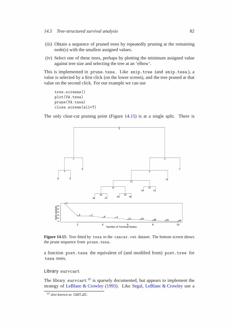
14.5 Tree-structured survival analysis 82
(iii) Obtain a sequence of pruned trees by repeatedly pruning at the remainingnode(s) with the smallest assigned values.
(iv) Select one of these trees, perhaps by plotting the minimum assigned valueagainst tree size and selecting the tree at an ‘elbow’.
This is implemented in prune.tssa . Like snip.tree (and snip.tssa ), avalue is selected by a first click (on the lower screen), and the tree pruned at thatvalue on the second click. For our example we can use
tree.screens()plot(VA.tssa)prune(VA.tssa)close.screen(all=T)
The only clear-cut pruning point (Figure 14.15) is at a single split. There is
|
8 9
5
96 9798 99
50 51
13
7
1
2
4
3
6
12
24
48 49
25
•••••••
••
•
Number of Terminal Nodes
Spl
it-st
atis
tic
2 4 6 8 10
12
34
56
492548241246
23
1
Figure 14.15: Tree fitted by tssa to the cancer.vet dataset. The bottom screen showsthe prune sequence from prune.tssa .
a function post.tssa the equivalent of (and modified from) post.tree fortssa trees.
Library survcart
The library survcart 10 is sparsely documented, but appears to implement thestrategy of LeBlanc & Crowley (1993). Like Segal, LeBlanc & Crowley use a
10 also known as CART SD .

14.5 Tree-structured survival analysis 83
goodness of split criterion for growing the tree, in this case the log-rank statisticwith some adjustment for selecting the maximal statistic over all possible splits ofcontinuous variables. However, the pruning strategy differs from tssa . Associateto each non-terminal node the goodness-of-split statistic G(`) , taking G to be zeroat the terminal nodes. Then LeBlanc & Crowley apply cost-complexity pruningto the measure of fit
R(T ) = −∑`∈T
G(`)
This is not a sum over cases, but as it is defined additively over branches thestandard pruning algorithm (Breiman et al., 1984; Ripley, 1996) is still justified.(The ‘deviance’ quoted by prune.survtree is
∑`G(`) .) The measure of fit
can be computed on a validation set based down the optimally pruned tree sequence(Tr) , but as it is not a measure of performance there is no justification for thenchoosing the best fit; indeed R(T ) decreases monotonically as the tree is grown,since G(`) > 0 . The suggestion of LeBlanc & Crowley is to choose the pruningminimizing Rα(T ) on the validation set for α ∈ [2, 4] . (LeBlanc & Crowleyalso discuss using bootstrapping to bias-correct R(T ) computed on the trainingset prior to pruning.)
Library survcart can be very memory-hungry: it comes with an informativedemonstration that needs over 50Mb11 of virtual memory to run.
We can try our VA cancer example by
library(survcart, first=T)VA.st <- survtree(stime ~ treat + age + Karn + diag.time +
cell + prior,data=VA, status, fact.flag=c(F,T,T,T,F,F))
plot(prune.survtree(VA.st))
The argument fact.flag says which variables should be regarded as not factorsand included in the adjustment of the log-rank statistic for continuous variates(although a factor with many levels will give rise to very many more possiblesplits). The ‘deviance’ is −R(Tk) − αk(|Tk| − 1) !
We can reserve a validation set and use this for pruning by
set.seed(123); tr <- sample(nrow(VA), 90)VA1 <- VA[tr,]; VA2 <- VA[-tr,]VA.st1 <- update(VA.st, data=VA1)VA.st1.pr <- prune.survtree(VA.st1, newdata=VA2,
zensor.newdata=VA2$status)VA.st1.pr$size:[1] 12 11 10 9 8 5 4 3 2 1 0
$dev:[1] 36.6986 36.0633 35.1245 24.2267 24.2514 13.5163[7] 15.7134 15.5296 -16.7492 -8.2354 0.0000
11 on each of S-PLUS 3.3 for Windows and on Sun Solaris; over 100Mb on S-PLUS 4.0 forWindows

14.5 Tree-structured survival analysis 84
$k:[1] 0.000000 0.033653 0.048377 0.709060 0.733988 2.595874[7] 2.692954 3.346168 12.984497 13.469285 19.090138
Note that the size is the number of splits, one less than the number of leaves. Weneed to convert this to a split-complexity measure:
attach(VA.st1.pr)dev <- dev + k*size> dev - 2*size[1] 12.6986 14.4335 15.6082 12.6082 14.1233 16.4956 18.4853[8] 19.5681 5.2198 3.2339 0.0000
> dev - 4*size[1] -11.3014 -7.5665 -4.3918 -5.3918 -1.8767 6.4956[7] 10.4853 13.5681 1.2198 1.2339 0.0000
detach()
which suggests a tree with three splits
> prune(VA.st1, k=4)
1) root 90 192) cell:2,3 49 134) prior:0 40 0 *5) prior:10 9 0 *
3) cell:1,4 41 136) Karn<45 8 0 *7) Karn>45 33 0 *
Note how the selection penalty on continuous variables such as Karn reducestheir prominence.
We can explore the spread of predictions over splits in a manner similar tokm.tssa by picking values of k in
VA.st.tmp <- prune.survtree(VA.st, k=2)plot(surv.fit(VA$stime, VA$status, factor(VA.st.tmp$where)))
This shows the Kaplan-Meier estimates of survival at all the leaves, and by succes-sively reducing k we can see when the range of variation is no longer essentiallycovered.
The function graph.survtree allows various aspects of the tree model tobe plotted. The following call plots the median survival by node
graph.survtree(prune(VA.st, k=3.5), VA$stime, VA$status,xtile=0.5, interactive=F)
but it can also show the survival probability at a fixed time.
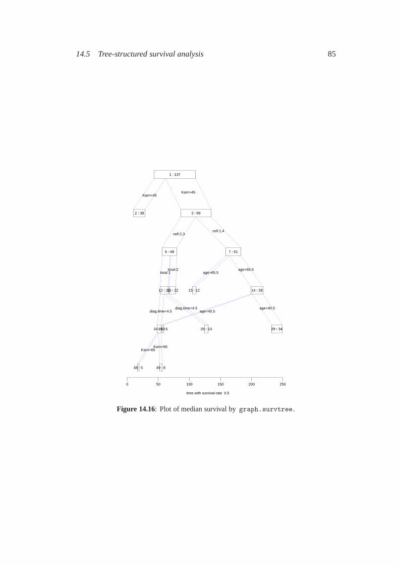
14.5 Tree-structured survival analysis 85
.
. .
.
.
.
. .
.
.
.
.
. .
.
time with survival-rate 0.5
0 50 100 150 200 250
1 : 137
2 : 38 3 : 99
6 : 48
12 : 26
24 : 13
48 : 5 49 : 8
25 : 13
13 : 22
7 : 51
14 : 39
28 : 5 29 : 34
15 : 12
Karn<45Karn>45
cell:2,3cell:1,4
treat:1treat:2
diag.time<4.5diag.time>4.5
Karn<65Karn>65
age>65.5age<65.5
age<40.5age>40.5
Figure 14.16: Plot of median survival by graph.survtree .

86
Chapter 15
Time Series
15.1 Second-order summaries
Spectral analysis
The most common approach to estimating a spectral density is to use a kernelsmoother, as implemented by spectrum , but there are alternatives, includingthe use of fitted high-order AR processes (page 448). One promising line is touse some of the alternative methods of estimating a probability density functionfunction, since a spectral density is just a finite multiple of a pdf.
The library lspec by Charles Kooperberg implements the logspline approachdescribed in Section 5.5 of these complements. Its application to spectral esti-mation is described in Kooperberg et al. (1995b); note that it is able to estimatemixed spectra that have purely periodic components. We will illustrate this byestimating the spectra of our running examples lh and deaths as well as theaccdeaths and nottem series.
For lh we have
> library(lspec)> lh.ls <- lspec.fit(lh)> lspec.summary(lh.ls)Logspline Spectral Estimation=============================The fit was obtained by the command:lspec.fit(data = lh)A spline with 3 knots, was fitted; there were no lines in the model.The log-likelihood of the model was 60.25 which corresponds to anAIC value of -110.96 .
The program went though 1 updown cycles, and reached a stablesolution. Both penalty (AIC) and minmass were the defaultvalues. For penalty this was log(n)=log( 24 )= 3.18 (as in BIC)and for minmass this was 0.0329. The locations of the knots were:1.178 2.749 3.142
> lspec.plot(lh.ls, log="y")> lspec.plot(lh.ls, what="p")

15.1 Second-order summaries 87
0.0 0.5 1.0 1.5 2.0 2.5 3.0
0.01
0.05
-3 -2 -1 0 1 2 3
0.0
0.10
0.20
0.30
Figure 15.25: Spectral density (left) and cumulative spectral distribution function (right)for the series lh computed by library lspec .
(Figure 15.25). Note that rather different conventions are used for the spectrum,which is taken to run over (−π, π] rather than in cycles, and the amplitude is givenin the normal units, not decibels. The spectral density and cumulative spectrumcan be found by dlspec and plspec respectively.
deaths.ls <- lspec.fit(deaths)lspec.plot(deaths.ls, log="y", main="deaths")lspec.plot(deaths.ls, what="p")accdeaths.ls <- lspec.fit(accdeaths)lspec.plot(accdeaths.ls, log="y", main="accdeaths")lspec.plot(accdeaths.ls, what="p")nott.ls <- lspec.fit(window(nottem, end=c(1936,12)))lspec.plot(nott.ls, log="y", main="nottem")lspec.plot(nott.ls, what="p")
(Figure 15.26). Note how lspec.fit finds the discrete component at frequencyπ/12 in all three cases, but is fooled by harmonics in the last two. We canallow lspec.fit to fit more discrete components by reducing the value of itsargument minmass (whose default can be found from lspec.summary ). In theaccdeaths example we can pick up all but one of the harmonics by
lspec.plot(lspec.fit(accdeaths, minmass=7000), log="y")lspec.plot(lspec.fit(accdeaths, minmass=1000), log="y")
but reducing minmass introduces discrete components at non-harmonic frequen-cies (Figure 15.27).
The functions clspec and rlspec compute the autocovariance (or autocor-relation) sequence corresponding to the fitted spectrum and simulate a Gaussiantime series with the fitted spectrum respectively.

15.1 Second-order summaries 88
deaths
0.0 0.5 1.0 1.5 2.0 2.5 3.0
5000
6000
7000
9000
2000
0
•
-3 -2 -1 0 1 2 3
010
0000
2000
0030
0000
accdeaths
0.0 0.5 1.0 1.5 2.0 2.5 3.0
5000
1000
050
0001
0000
050
0000
•
-3 -2 -1 0 1 2 3
020
0000
4000
0060
0000
8000
00
nottem
0.0 0.5 1.0 1.5 2.0 2.5 3.0
0.5
1.0
5.0
•
-3 -2 -1 0 1 2 3
020
4060
Figure 15.26: Spectral density (top) and cumulative spectral distribution function (bottom)for the series deaths , accdeaths and nottem .
0.0 0.5 1.0 1.5 2.0 2.5 3.0
5000
1000
050
0001
0000
050
0000
•
0.0 0.5 1.0 1.5 2.0 2.5 3.0
5000
1000
050
0001
0000
050
0000
•
• •
•
0.0 0.5 1.0 1.5 2.0 2.5 3.0
5000
1000
050
000
1000
0050
0000
•
• •• • • •
Figure 15.27: Spectra for nottem with minmass as (left to right) 77 000, 7000 and 1000.

89
Chapter 16
Spatial Statistics
16.3 Module S+SPATIALSTATS
The first release of the S-PLUS module S+SPATIALSTATS was released in mid-1996. That has a comprehensive manual (published as Kaluzny & Vega, 1997),which we do not aim to duplicate, but rather to show how our examples inChapter 16 can be done using S+SPATIALSTATS.
The module S+SPATIALSTATS is attached and made operational by
module(spatial)
which we will assume has been done. Unfortunately the name is the same as ourlibrary (as are some of the function names); modules take priority over libraries.
Kriging
The kriging functions use a slight extension of the model formula language. Thefunction loc is used to specify the two spatial coordinates of the points, whichare used to find the covariance matrix in kriging. Universal kriging is specified byadding other terms to form a linear model. Thus we can specify the model usedin the bottom row of Figure 16.5 by
> topo.kr <- krige(z ~ loc(x, y) + x + y + x^2 + x*y + y^2,data=topo, covfun=exp.cov, range=0.7, sill=770)
> topo.kr....
Coefficients:constant x y x^2 xy y^2
808.3 -12.896 -64.486 62.137 1.6332 6.3442....
> prsurf <- predict(topo.kr, se.fit = T,grid = list(x=c(0, 6.5, 50), y=c(0, 6.5, 50)))
> topo.plt1 <- contourplot(fit ~ x*y, data=prsurf, pretty=F,at=seq(700, 1000, 25), aspect=1,panel = function(...){
panel.contourplot(...)points(topo)

16.3 Module S+SPATIALSTATS 90
})> topo.plt2 <- contourplot(se.fit ~ x*y, data=prsurf, pretty=F,
at=c(20, 25), aspect=1)> print(topo.plt1, split=c(1,1,2,1), more=T)> print(topo.plt2, split=c(2,1,2,1))
(The sill value is explained below.) We can of course obtain a least-squarestrend surface by giving a covariance function that drops to zero immediately, forexample exp.cov with range = 0 , but there seems no simple way to obtain atrend surface fitted by GLS. The predict method for krige objects takes eithera newdata argument or a grid argument as used here. The grid argumentmust be a list with two components with names matching those given to locand specifying the minimum, maximum and number of points. (This is passed toexpand.grid to compute a data frame for newdata .)
Analogues of the fits shown in Figure 16.6 may be obtained by
topo.kr2 <- krige(z ~ loc(x, y) + x + y + x^2 + x*y + y^2,data = topo, covfun = gauss.cov,range = 1, sill = 600, nugget = 100)
topo.kr3 <- krige(z ~ loc(x, y), data = topo,covfun = gauss.cov, range = 2, sill = 6500, nugget = 100)
Various functions are provided to fit variograms and correlograms. We startby fitting a variogram to the original data.
topo.var <- variogram(z ~ loc(x, y), data=topo)model.variogram(topo.var, gauss.vgram, range=2,
sill=6500, nugget=100)
The function model.variogram plots the variogram object (which may alsobe plotted directly) and draws a theoretical variogram. It then prompts the userto alter the parameters of the variogram to obtain a good fit by eye. It thiscase range = 3.5 seems indicated. The parametrization is that nugget is theincrement at the origin, and sill is the change over the range of increase of thevariogram. (In geostatistical circles the sum of ‘nugget’ and ‘sill’ is called thesill.) Thus the alph of our covariance functions is nugget/(sill + nugget) .
There are functions correlogram and covariogram which can be used inthe same way (including with model.variogram ).
topo.cov <- covariogram(z ~ loc(x, y), data=topo)model.variogram(topo.cov, gauss.cov, range=2,
sill=4000, nugget=2000)
We can now explain how we chose the the parameters of the exponentialcovariance in the first plot. An object of class "krige" contains residuals, so wecan use
topo.ls <- krige(z ~ loc(x, y) + x + y + x^2 + x*y + y^2,data=topo, covfun=exp.cov, range=0)
topo.res <- residuals(topo.ls)topo.var <- variogram(topo.res ~ loc(x, y), data=topo)model.variogram(topo.var, exp.vgram, range=1, sill=1000)

16.3 Module S+SPATIALSTATS 91
0
2000
4000
6000
80000
0 1 2 3 4
90
0 1 2 3 4
distance
gam
ma
0
500
1000
1500
0
0 1 2 3 4
90
0 1 2 3 4
distance
gam
ma
Figure 16.10: Directional variograms for the topo dataset. The top pair is for the rawdata, the bottom pair of residuals from a quadratic trend surface. The left plots are verticalvariograms, the right plots are horizontal ones. (The strip coverage is misleading, onlyshowing the positive part of the angular tolerance.)
This suggests a sill of about 800. The kriging predictions do not depend on thesill, and our spatial library relies on this to work throughout with correlogramsand to fit the overall scale factor when plotting the standard errors. Knowledge ofour code allowed us to read off the value 770. It would be a good idea to repeatthe forming of the residuals, this time from the GLS trend surface. We can choosethe covariogram for the Gaussian case in the same way.
topo.var <- covariogram(topo.res ~ loc(x, y), data=topo)model.variogram(topo.var, gauss.cov, range=1, sill=210,
nugget=90)
Spatial anisotropy
The geostatistical functions in S+SPATIALSTATS have considerable support forstudying anisotropy of smooth spatial surfaces, and to correct for geometricalanisotropy (anisotropy which can be removed by ‘squeezing’ the plot in somedirection). The function loc has two additional parameters angle and ratioto remove geometrical anisotropy. The functions variogram , correlogram andcovariogram all allow multiple plots for pairs of distances in angular sectors.For example
plot(variogram(z ~ loc(x, y), data=topo, azimuth = c(0, 90),tol.azimuth = 45), aspect=0.7, layout=c(2,1))
plot(variogram(topo.res ~ loc(x, y), data=topo,

16.3 Module S+SPATIALSTATS 92
azimuth = c(0, 90), tol.azimuth = 45),aspect=0.7, layout=c(2,1))
They show vertical and horizontal variograms (for pairs within a tolerance of±45◦ ) of the raw topo data and then the residuals from the quadratic trendsurface. (As these produce and print Trellis plots, none of the normal ways toput two plots on one page are possible and Figure 16.10 is assembled from twoS-PLUS plots.)
Point process functions
Spatial point patterns are objects of class "spp" , with constructor function spp .We can convert our pines.dat to a spp object by
library(spatial) # our library, for next line only.pines <- data.frame(ppinit("pines.dat")[c("x", "y")])pines <- spp(pines, "x", "y", bbox(c(0,9.6), c(0, 10)), drop=T)attributes(pines)$class:[1] "spp" "data.frame"$coords:[1] "x" "y"$boundary:$boundary$x:[1] 0.0 0.0 9.6 9.6$boundary$y:[1] 10 0 0 10
An object of class "spp" is a data frame with two attributes, "coords" declareswhich columns give the spatial coordinates, and "boundary" which gives theboundary of a polygon within which the pattern was observed. (This defaults tothe bounding rectangle aligned with the axes, but the use of that is not advisable.)
We can reproduce Figure 16.8 quite closely by
par(pty = "s", mfrow=c(2,2))plot(pines, boundary = T)Lhat(pines, maxdist = 5)Lenv(pines, 25, process = "binomial", maxdist=5)Lhat(pines, maxdist =1.5)Lenv(pines, 100, process = "Strauss", maxdist = 1.5,
cpar = 0.2, radius = 0.7)
As this code shows, Lenv can simulate from several point process models: itdoes so by calling the function make.pattern whose functionality is equivalentto that of our functions Psim , SSI and Strauss plus certain Poisson clusterprocesses.
There is no way to estimate parameters of point process models in the currentrelease of S+SPATIALSTATS, but it does have functions Fhat and Ghat to usenearest neighbour methods, and function intensity to estimate the intensityfunction of a heterogeneous point process. (This is closely related to bivariatedensity estimation.)

93
Chapter 17
Classification
17.3 Forensic glass
Neural networks
The recently-added method nnet.formula allows us to write some generalfunctions for testing neural network models by V -fold cross-validation. First were-scale the dataset so the inputs have range [0, 1] .
fgl1 <- lapply(fgl[, 1:9], function(x){r <- range(x); (x-r[1])/diff(r)})
fgl1 <- data.frame(fgl1, type=fgl$type)
Then we can experiment with multiple logistic regressions.
res.multinom <- CVtest(function(x, ...) multinom(type ~ ., fgl1[x,], ...),function(obj, x) predict(obj, fgl1[x, ],type="class"),maxit=1000, trace=F)
con(fgl$type, res.multinom)
We can now use a modest amount of weight decay as ‘ridge regression’, to reducethe effects of any irrelevant inputs.
res.mult2 <- CVtest(function(x, ...) multinom(type ~ ., fgl1[x,], ...),function(obj, x) predict(obj, fgl1[x, ], type="class"),maxit=1000, trace=F, decay=1e-3)
> con(fgl$type, res.mult2)....
error rate = 36.45 %
and also try out subset selection by
res.mult3 <- CVtest(function(xsamp, ...) {assign("xsamp", xsamp, frame=1)obj <- multinom(type ~ ., fgl1[xsamp,], trace=F, ...)stepAIC(obj)

17.3 Forensic glass 94
},function(obj, x) predict(obj, fgl1[x, ],type="class"),maxit=1000, decay=1e-3)
> con(fgl$type, res.mult3)....
error rate = 41.12 %
In our runs the variables RI , Na , Mg , Al and Si were retained in all 10 folds,and Ca in all but one, the only one in which K and Ba were retained.
It is straightforward to fit a fully specified neural network in the same way.
res.nn <- CVtest(function(x, ...) nnet(type ~ ., fgl1[x,], ...),function(obj, x) predict(obj, fgl1[x, ], type="class"),maxit=1000, size=6, decay=0.01, trace=F )
> con(fgl$type, res.nn)....
error rate = 29.91 %
We will, however, want to average across several fits
CVnn <- function(nreps=1, ...){
res <- matrix(0, 214, 6)dimnames(res) <- list(NULL, levels(fgl$type))for (i in sort(unique(rand))) {cat("fold ",i,"\n", sep="")for(rep in 1:nreps) {learn <- nnet(type ~ ., fgl1[rand !=i,], trace=F, ...)res[rand == i,] <- res[rand == i,] +predict(learn, fgl1[rand==i,])
}}max.col(res/nreps)
}> res.nn <- CVnn(maxit=1000, size=6, decay=0.01)> con(fgl$type, res.nn)
....error rate = 29.44 %
and to choose the number of hidden units and the amount of weight decay by aninner cross-validation. To do so we wrote fairly general function that can easilybe used or modified to suit other problems.
CVnn2 <- function(formula, data,size = rep(6,2), lambda = c(0.001, 0.01),nreps = 1, nifold = 5, verbose = 99, ...)
{CVnn1 <- function(formula, data, nreps=1, ri, verbose, ...){truth <- data[,deparse(formula[[2]])]

17.3 Forensic glass 95
res <- matrix(0, nrow(data), length(levels(truth)))if(verbose > 20) cat(" inner fold")for (i in sort(unique(ri))) {if(verbose > 20) cat(" ", i, sep="")for(rep in 1:nreps) {learn <- nnet(formula, data[ri !=i,], trace=F, ...)res[ri == i,] <- res[ri == i,] +predict(learn, data[ri == i,])
}}if(verbose > 20) cat("\n")sum(unclass(truth) != max.col(res/nreps))
}truth <- data[,deparse(formula[[2]])]res <- matrix(0, nrow(data), length(levels(truth)))choice <- numeric(length(lambda))for (i in sort(unique(rand))) {if(verbose > 0) cat("fold ", i,"\n", sep="")ri <- sample(nifold, sum(rand!=i), replace=T)for(j in seq(along=lambda)) {if(verbose > 10)cat(" size =", size[j], "decay =", lambda[j], "\n")
choice[j] <- CVnn1(formula, data[rand != i,], nreps=nreps,ri=ri, size=size[j], decay=lambda[j],verbose=verbose, ...)
}decay <- lambda[which.is.max(-choice)]csize <- size[which.is.max(-choice)]if(verbose > 5) cat(" #errors:", choice, " ")if(verbose > 1) cat("chosen size = ", csize,
" decay = ", decay, "\n", sep="")for(rep in 1:nreps) {learn <- nnet(formula, data[rand != i,], trace=F,
size=csize, decay=decay, ...)res[rand == i,] <- res[rand == i,] +
predict(learn, data[rand == i,])}
}factor(levels(truth)[max.col(res/nreps)],
levels = levels(truth))}> res.nn2 <- CVnn2(type ~ ., fgl1, skip=T, maxit=500, nreps=10)> con(fgl$type, res.nn2)
WinF WinNF Veh Con Tabl HeadWinF 57 10 3 0 0 0
WinNF 16 51 3 4 2 0Veh 8 3 6 0 0 0Con 0 3 0 9 0 1
Tabl 0 1 0 1 5 2Head 0 3 0 1 0 25

17.3 Forensic glass 96
error rate = 28.5 %
This fits a neural network 1000 times, and so is fairly slow (6 hours on the PC)and memory-intensive (about 20 Mb).
This code chooses between neural nets on the basis of their cross-validatederror rate. An alternative is to use logarithmic scoring, which is equivalent tofinding the deviance on the validation set. Rather than count 0 if the predictedclass is correct and 1 otherwise, we count − log p(c |x) for the true class c . Wecan easily code this variant by replacing the line
sum(unclass(truth) != max.col(res/nreps))
by
sum(-log(res[cbind(seq(along=truth),unclass(truth))]/nreps))
Learning vector quantization
For LVQ as for k -nearest neighbour methods we have to select a suitable metric.The following experiments used Euclidean distance on the original variables, butthe rescaled variables or Mahalanobis distance could also be tried.
cd0 <- lvqinit(fgl0, fgl$type, prior=rep(1,6)/6,k=3)cd1 <- olvq1(fgl0, fgl$type, cd0)con(fgl$type, lvqtest(cd1, fgl0))
We set an even prior over the classes as otherwise there are too few representativesof the smaller classes. Our initialization code follows Kohonen’s in selecting thenumber of representatives: in this problem 24 points are selected, four from eachclass.
CV.lvq <- function(){
res <- fgl$typefor(i in sort(unique(rand))) {cat("doing fold",i,"\n")cd0 <- lvqinit(fgl0[rand != i,], fgl$type[rand != i],
prior=rep(1,6)/6, k=3)cd1 <- olvq1(fgl0[rand != i,], fgl$type[rand != i], cd0)cd1 <- lvq3(fgl0[rand != i,], fgl$type[rand != i],
cd1, niter=10000)res[rand == i] <- lvqtest(cd1, fgl0[rand == i,])
}res
}con(fgl$type, CV.lvq())
WinF WinNF Veh Con Tabl HeadWinF 59 10 1 0 0 0
WinNF 10 61 1 2 2 0Veh 6 8 3 0 0 0

17.3 Forensic glass 97
Con 0 2 0 6 2 3Tabl 0 0 0 2 7 0Head 3 2 0 1 1 22
error rate = 26.17 %
# Try Mahalanobis distancefgl0 <- scale(princomp(fgl[,-10])$scores)con(fgl$type, CV.lvq())
....error rate = 35.05 %
The initialization is random, so your results are likely to differ.
Additive and tensor-spline models
The additive models discussed in Section 11.1 of these complements can alsobe used for classification problems. Three approaches to using a flexible familyg(x; θ) of functions for classification are discussed in Ripley (1996, Chapter 4),and we can use each of them for this problem.
Least-squares fitting to indicator functions
In this approach the K classes generate an N ×K indicator matrix Y , which isregressed on the flexible family. The indicator matrix can easily be generated bythe function class.ind in library nnet . Thus we can use BRUTO by
library(mda); library(nnet)levs <- levels(fgl$type)fgl.bruto <- bruto(fgl[, 1:9], class.ind(fgl$type))bruto.class <- max.col(predict(fgl.bruto, as.matrix(fgl[, 1:9])))con(fgl$type, factor(levs[bruto.class], levels=levs))
In this approach it is conventional to classify by predicting the class whose indicatoris nearest to the vector prediction: elementary algebra shows that this is the sameas choosing the largest of the predictions.
To obtain comparable results we need to use cross-validation.
res.bruto <- CVtest(function(xsamp, ...)bruto(fgl[xsamp, 1:9], class.ind(fgl$type)[xsamp,], ...),
function(obj, x)factor(levs[max.col(predict(obj,
as.matrix(fgl[x, 1:9])))], levels=levs))con(fgl$type, res.bruto)
....error rate = 34.11 %
Class Veh was never selected.Almost exactly the same code can be used with MARS. We try additive
models, then pairwise and then general tensor products.

17.3 Forensic glass 98
res.mars <- CVtest(function(xsamp, ...)mars(as.matrix(fgl[xsamp, 1:9]),
class.ind(fgl$type)[xsamp,], ...),function(obj, x)factor(levs[max.col(predict(obj,
as.matrix(fgl[x, 1:9])))], levels=levs))con(fgl$type, res.mars)
....error rate = 35.98 %
res.mars2 <- CVtest(degree=2,function(xsamp, ...)mars(as.matrix(fgl[xsamp, 1:9]),
class.ind(fgl$type)[xsamp,], ...),function(obj, x)factor(levs[max.col(predict(obj,
as.matrix(fgl[x, 1:9])))], levels=levs))con(fgl$type, res.mars2)
....error rate = 33.64 %
res.mars9 <- CVtest(degree=9,function(xsamp, ...)mars(as.matrix(fgl[xsamp, 1:9]),
class.ind(fgl$type)[xsamp,], ...),function(obj, x)factor(levs[max.col(predict(obj,
as.matrix(fgl[x, 1:9])))], levels=levs))con(fgl$type, res.mars9)
....error rate = 34.11 %
The library polymars of Kooperberg and O’Connor implements a restrictiveform of MARS (for example, allowing only pairwise interations) suggested byKooperberg et al. (1997), but will automatically generate the necessary indicatorfunctions.
Prediction followed by linear discriminant analysis
Breiman & Ihaka (1984) had an idea to use a flexible family within linear discrim-inant analysis. This was picked up by Hastie et al. (1994) and Ripley (1994b); afull explanation of the connections is given in Ripley (1996). The idea amounts tousing a least-squares prediction as above, but using linear discriminant analysis onthe outputs, rather than choosing the largest output. Hastie et al. call this ‘flexiblediscriminant analysis’.

17.3 Forensic glass 99
The function fda in library mda can be used to implement this procedure.This does use formulae.
library(mda)res.bruto.fda <- CVtest(method=bruto,
function(xsamp, ...)fda(type ~ ., data=fgl[xsamp,], ...),
function(obj, x) predict(obj, fgl[x, ]))con(fgl$type, res.bruto.fda)
....error rate = 34.58 %
res.mars.fda <- CVtest(method=mars,function(xsamp, ...)fda(type ~ ., data=fgl[xsamp,], ...),
function(obj, x) predict(obj, fgl[x, ]))con(fgl$type, res.mars.fda)
....error rate = 35.51 %
res.mars2.fda <- CVtest(method=mars, degree=2,function(xsamp, ...)fda(type ~ ., data=fgl[xsamp,], ...),
function(obj, x) predict(obj, fgl[x, ]))con(fgl$type, res.mars2.fda)
....error rate = 38.32 %
res.mars9.fda <- CVtest(method=mars, degree=9,function(xsamp, ...)fda(type ~ ., data=fgl[xsamp,], ...),
function(obj, x) predict(obj, fgl[x, ]))con(fgl$type, res.mars9.fda)
....error rate = 34.58 %
Non-linear logistic discrimination
The third approach is a non-linear logistic model, that is
p(C = c |X = x) =exp gc(x; θ)∑i exp gi(x; θ)
(17.2)
This is the approach taken by nnet with argument softmax=T . Note that thereis some redundancy in (17.2) since the fitted probabilities depend only on thedifferences between the coordinates of g .
Library polyclass 1 by Charles Kooperberg fits (17.2) by additive models1 polyclas on Windows.

17.3 Forensic glass 100
with linear splines and can also include pairwise interactions. (Thus its space ofnon-linear functions is the same as that used by MARS with degree=2 .) Theredundancy is resolved by taking gK ≡ 0 . The methodology is described in moredetail by Kooperberg et al. (1997) and Stone et al. (1997).
Fits using the polyclass library can be very slow. In the following codewe reduce the maximum dimension of model fitted to achieve a more reasonableresponse time (about 2 minutes) after monitoring some preliminary runs (withparameter silent=F ).
library(polyclass)res.polycl <- CVtest(maxdim=50,
function(xsamp, ...)poly.fit(unclass(fgl$type)[xsamp],
as.matrix(fgl[xsamp, 1:9]), ...),function(obj, x)factor(levs[max.col(ppoly(fit=obj,
cov=as.matrix(fgl[x, 1:9])))],levels=levs)
)con(fgl$type, res.polycl)
....error rate = 34.58 %
By default poly.fit uses a penalty on the number of terms used, in a similar wayto logspline . If the argument cv is set to V it uses V -fold cross-validationto choose the complexity.
res.polycl2 <- CVtest(maxdim=50, cv=10, seed=123,function(xsamp, ...)poly.fit(unclass(fgl$type)[xsamp],
as.matrix(fgl[xsamp, 1:9]), ...),function(obj, x)factor(levs[max.col(ppoly(fit=obj,
cov=as.matrix(fgl[x, 1:9])))],levels=levs)
)con(fgl$type, res.polycl2)
....error rate = 31.78 %
This fit took 17 minutes on the PC. The answer depends on the random partition;this is selected by the seed parameter (see the help page for the details).
The function poly.summary provides extensive information on a fitted poly-class model, and poly.beta and poly.plot plots aspects of the model.
Mixture discriminant analysis
‘Mixture discriminant analysis’ (Hastie & Tibshirani, 1996) is a variant on plug-inlinear discriminant analysis in which a mixture of normals is fitted to each class,

17.4 Cross-validation 101
all normals having a common covariance matrix. This can be fitted by the functionmda in library mda . We chose varying numbers of components depending on theprevalence of each class. The initialization is random, so your results may differ.
library(class) # needed for the initializationres.mda <- CVtest(subclasses=c(6,6,3,3,2,4),
function(xsamp, ...)mda(type ~ ., data=fgl[xsamp,], ...),
function(obj, x) predict(obj, fgl[x, ]))con(fgl$type, res.mda)
....error rate = 30.84 %
This took about 4 minutes.
17.4 Cross-validation
We have several uses of V-fold cross-validation in this chapter, as well as inselecting the complexity parameter when pruning classification trees. The codegiven on page 493 is reasonably general, and can be used for cross-validation ofany procedure with a fitting function and a predict method that returns a relativelysimple result (such as a classifcation factor or a matrix of probabilities. We canuse something like
rand <- sample(V, nrow(data), replace=T)CVtest <- function(fitfn, predfn, ...){
res <- data$responsefor (i in sort(unique(rand))) {
cat("fold ",i,"\n", sep="")learn <- fitfn(rand != i, ...)res[rand == i] <- predfn(learn, rand==i)NULL
}res
}
(We added a NULL at the end of the loop as in sp 3.x this can help in minimizingmemory usage.) For example, to find cross-validated posterior probabilities forlinear discriminant anaysis of the iris data we would use
ir <- rbind(iris[,,1], iris[,,2], iris[,,3])ir.species <- c(rep("s",50), rep("c",50), rep("v",50))V <- 10rand <- sample(V, nrow(ir), replace=T)CVtest <- function(fitfn, predfn, ...){
res <- matrix(nrow=nrow(ir), ncol=3)

17.4 Cross-validation 102
for (i in sort(unique(rand))) {cat("fold ",i,"\n", sep="")learn <- fitfn(rand != i, ...)res[rand == i,] <- predfn(learn, rand==i)NULL
}res
}res.lda <- CVtest(
function(x, ...) lda(ir.species, ir, subset=x, ...),function(obj, x) predict(obj, ir[x, , drop=F])$post )
)
In general such cross-validated results can be quite variable, and we say for theuse of cross-validation with classification trees, it can be helpful to average theresults across a several different random partitions if CPU time permits.
What may not be obvious is that exactly the same code can be used for theearlier technique of leave-one-out cross-validation: just use
rand <- 1:nrow(ir)
Leave-one-out cross-validation is not generally to be recommended: it has con-siderable disadvantages, principally in giving highly-variable results and for somefitting procedures in not making a sufficient perturbation to the problem, for exam-ple when variable selection is used. Nevertheless, it may be of historical interest,and as for programming exercise we have added an argument CV=T to both ldaand qda that invokes the fast updating formulae given2 in Ripley (1996, p. 100).
Leave-one-out cross-validation is of much greater interest for a nearest-neighbourclassifier. The function knn.cv in library class implements this in the straight-forward way (by removing to considering each point when searching for its neigh-bours).
2 see its Errata for typographical corrections

103
References
Basilevsky, A. (1994) Statistical Factor Analysis and Related Methods. New York: JohnWiley and Sons. 65
Bowman, A. and Azzalini, A. (1997) Applied Smoothing Techniques for Data Analysis:The Kernel Approach with S-Plus Illustrations. Oxford: Oxford University Press. 1,37, 43, 57
Breiman, L., Friedman, J. H., Olshen, R. A. and Stone, C. J. (1984) Classification andRegression Trees. Monterey: Wadsworth and Brooks/Cole. 67, 83
Breiman, L. and Ihaka, R. (1984) Nonlinear discriminant analysis via ACE and scaling.Technical Report 40, Dept of Statistics, University of California, Berkeley. 98
Ciampi, A., Chang, C.-H., Hogg, S. and McKinney, S. (1987) Recursive partitioning: aversatile method for exploratory data analysis in biostatistics. In Biostatistics, eds I. B.McNeil and G. J. Umphrey, pp. 23–50. New York: Reidel. 79
Darroch, J. N. and Ratcliff, D. (1972) Generalized iterative scaling for log-linear models.Annals of Mathematical Statistics 43, 1470–1480. 13
Davis, R. and Anderson, J. (1989) Exponential survival trees. Statistics in Medicine 8,947–961. 79
Davison, A. C. and Hinkley, D. V. (1997) Bootstrap Methods and Their Application.Cambridge: Cambridge University Press. 8, 9, 23
Efron, B. and Tibshirani, R. (1993) An Introduction to the Bootstrap. New York: Chapmanand Hall. 10
Ein-Dor, P. and Feldmesser, J. (1987) Attributes of the performance of central processingunits: A relative performance prediction model. Communications of the ACM 30,308–317. 39
Friedman, J. H. (1984) SMART user’s guide. Technical Report 1, Laboratory for Compu-tational Statistics, Dept of Statistics, Stanford University. 44
Friedman, J. H. (1991) Multivariate adaptive regression splines (with discussion). Annalsof Statistics 19, 1–141. 39
Gower, J. C. and Hand, D. J. (1996) Biplots. London: Chapman & Hall. 62, 64
Gray, R. J. (1994) Hazard estimation with covariates: algorithms for di-rect estimation, local scoring and backfitting. Technical Report 784Z,Dana-Farber Cancer Institute, Division of Biostatistics. [ Available fromftp://farber.harvard.edu/stats/gray/784Z.ps.Z ]. 58, 59
Gray, R. J. (1996) Hazard rate regression using ordinary nonparametric regressionsmoothers. J. Comp. Graph. Statist. 5, 190–207. 58
Greenacre, M. (1992) Correspondence analysis in medical research. Statistical Methods inMedical Research 1, 97–117. 63, 64
Hastie, T. and Tibshirani, R. (1996) Discriminant analysis by Gaussian mixtures. Journalof the Royal Statistical Society series B 58, 158–176. 100

References 104
Hastie, T., Tibshirani, R. and Buja, A. (1994) Flexible discriminant analysis by optimalscoring. Journal of the American Statistical Association 89, 1255–1270. 98
Hastie, T. J. and Tibshirani, R. J. (1990) Generalized Additive Models. London: Chapmanand Hall. 39
Hjort, N. L. (1997) Dynamic likelihood hazard rate estimation. Biometrika 84, xxx–xxx.55
Jolliffe, I. T. (1986) Principal Component Analysis. New York: Springer-Verlag. 65
Kaluzny, S. and Vega, S. C. (1997) S+SPATIALSTATS. New York: Springer-Verlag. 89
Kooperberg, C., Bose, S. and Stone, C. J. (1997) Polychotomous regression. Journal of theAmerican Statistical Association 92, 117–127. 39, 98, 100
Kooperberg, C. and Stone, C. J. (1992) Logspline density estimation for censored data.Journal of Computational and Graphical Statistics 1, 301–328. 1
Kooperberg, C., Stone, C. J. and Truong, Y. K. (1995a) Hazard regression. J. Amer. Statist.Assoc. 90, 78–94. 56, 59, 60
Kooperberg, C., Stone, C. J. and Truong, Y. K. (1995b) Logspline estimation for a possiblemixed spectral distribution. Journal of Time Series Analysis 16, 359–388. 86
LeBlanc, M. and Crowley, J. (1992) Relative risk trees for censored survival data. Biometrics48, 411–425. 68
LeBlanc, M. and Crowley, J. (1993) Survival trees by goodness of split. Journal of theAmerican Statistical Association 88, 857–867. 82, 83
Loader, C. R. (1995) Old faithful erupts: Bandwidth selection reviewed. Tech-nical Report 95.9, Bell Laboratories, Murray Hill, NJ. [ Available fromhttp://cm.bell-labs.com/stat/doc/95.9.ps ]. 7
Loader, C. R. (1996) Local likelihood density estimation. Annals of Statistics 24, 1602–1618. 4
Loader, C. R. (1997) Locfit: An introduction. Statistical Computing and Graphics Newslet-ter [Available from http://cm.bell-labs.com/stat/project/locfit]. 4, 5, 37
McCullagh, P. and Nelder, J. A. (1989) Generalized Linear Models. Second Edition.London: Chapman and Hall. 18, 19
Ripley, B. D. (1994a) Neural networks and flexible regression and discrimination. InStatistics and Images 2, ed. K. V. Mardia, volume 2 of Advances in Applied Statistics,pp. 39–57. Abingdon: Carfax. 39
Ripley, B. D. (1994b) Neural networks and related methods for classification (with discus-sion). Journal of the Royal Statistical Society series B 56, 409–456. 98
Ripley, B. D. (1996) Pattern Recognition and Neural Networks. Cambridge: CambridgeUniversity Press. 44, 78, 79, 83, 97, 98, 102
Ruppert, D., Sheather, S. J. and Wand, M. P. (1995) An effective bandwidth selector forlocal least squares regression. Journal of the American Statistical Association 90,1257–1270. 37
Segal, M. R. (1988) Regression trees for censored data. Biometrics 44, 35–47. 80, 81, 82
Simonoff, J. S. (1996) Smoothing Methods in Statistics. New York: Springer. 1, 37
Stone, C. J., Hansen, M., Kooperberg, C. and Truong, Y. K. (1997) Polynomial splines andtheir tensor products in extended linear modelling. Annals of Statistics 25, 1371–1470.1, 100
Tarone, R. E. and Ware, J. (1977) On distribution-free tests for the equality of survivaldistributions. Biometrika 64, 156–160. 80

References 105
Therneau, T. M. and Atkinson, E. J. (1997) An introduction to recursive partitioning usingthe RPART routines. Technical report, Mayo Foundation. [Distributed in PostScriptwith the RPART package.]. 67
Wahba, G., Gu, C., Wang, Y. and Chappell, R. (1995) Soft classification a.k.a. risk es-timation via penalized log likelihood and smoothing spline analysis of variance. InThe Mathematics of Generalization, ed. D. H. Wolpert, pp. 331–359. Reading, MA:Addison-Wesley. 44
Wand, M. P. and Jones, M. C. (1995) Kernel Smoothing. Chapman & Hall. 37, 55

106
Index
Entries in this font are names of S objects.
accdeaths, see Datasetsadditive models, 37, 97–100Aids, see Datasets
BCa confidence intervals, 9bcanon, 11BIC, 25biplot, 63biplot.correspondence, 63birthwt, see Datasetsboot, 8–10boot.ci, 8, 9bootstrap, 8, 22
parametric, 9bootstrap, 9–11boott, 11bruto, 39, 40
cancer.vet, see DatasetsCars93, see Datasetscensboot, 9class.ind, 97clspec, 87coop, see DatasetscorClasses, 29correlogram, 90correlogram, 90, 91corresp, 63correspondence analysis, 62
multiple, 64plots, 63
covariogram, 90, 91cpus, see Datasetscross-validation, 93, 94, 101
leave-one-out, 102crosstabs, 16cv.tree, 67
Datasetsaccdeaths, 86–88
Aids, 56, 57birthwt, 43, 44cancer.vet, 59, 60, 74, 81, 82Cars93, 16coop, 27cpus, 39, 47, 68, 69deaths, 86, 88faithful, 2, 5fgl, 93galaxies, 3, 4, 7, 8gehan, 55, 56heart, 57iris, 68, 69, 74, 101lh, 86, 87mcycle, 37, 38minn38, 14nottem, 88oats, 26petrol, 24Pima, 44quine, 17, 20rock, 45, 46, 48–50sitka, 27, 30topo, 89, 91, 92
deaths, see Datasetsdensity estimation
local polynomial, 4–7logspline, 1–3
denumerate, 17digamma function, 18discriminant analysis
flexible, 98mixture, 100
dispersion parameter, 18dlogspline, 3dlspec, 87
erase.screen, 81expand.grid, 90experiments

Index 107
split-plot, 26
faithful, see Datasetsfda, 98fgl, see DatasetsFhat, 92flexible discriminant analysis, 98forensic glass, 93
galaxies, see Datasetsgam, 41gamma family, 18gehan, see Datasetsgeneralized linear models
gamma family, 18Ghat, 92glm.dispersion, 19glm.shape, 19gls, 35graph.survtree, 84, 85
hare.fit, 59hazcov, 58heart, see Datasetsheft.fit, 56, 57, 60
iris, 71iris, see Datasetsiterative proportional scaling, 12
km.tssa, 81, 84knn.cv, 102krige, 89kriging, 89
learning vector quantization, 96Lenv, 92library
boot, 8, 9, 23bootstra, 10class, 102hare, 59hazcov, 58heft, 56KernSmooth, 4, 37ksmooth, 4, 37locfit, 4, 37, 43, 56logspline, 1, 55lspec, 86, 87MASS, 13, 19
mda, 39, 98, 100multinom, 50nlme, 24, 32, 35nnet, 49, 50, 97polyclass, 99, 100polymars, 39, 98ppr, 45rpart, 67, 79sm, 1, 37, 43, 57survcart, 82, 83tssa, 80
linear mixed effects models, 24–29lme, 24–29, 35, 36loadings, 65
correlation, 65loc, 89, 91locfit, 4–8, 38, 43, 44, 56, 58locpoly, 4, 38loess, 43, 58log-linear models, 12logarithmic scoring, 96logistic regression, 93loglin, 12–14, 16, 17loglm, 13–17logspline.fit, 2, 3, 56logspline.plot, 3logspline.summary, 3lspec.fit, 86, 87lspec.plot, 86lspec.summary, 87LVQ, 96
mars, 39, 40mca, 64mcycle, see Datasetsmda, 100minn38, see Datasetsmixed effects models
linear, 24–29non-linear, 30–35
mixture discriminant analysis, 100model formulae, 89model.variogram, 90multinom, 49, 50
na.rpart, 78nearest-neighbour, 102neural networks, 49, 93nlme, 30, 32nls, 32

Index 108
nnet, 49, 52, 99nnet.default, 49, 51nnet.formula, 49–51, 93nnet.Hess, 49non-linear mixed effects models, 30–
35non-linear models
self-starting, 32nottem, see Datasets
oats, see Datasets
petrol, see DatasetsPima, see Datasetsplogspline, 3plot.corresp, 63plot.rpart, 76plotcp, 70, 75plspec, 87point processes, 92Poisson log-linear model, 12poly.beta, 100poly.fit, 100poly.plot, 100poly.summary, 100polyclass models, 100post, 76post.rpart, 76post.tree, 76post.tssa, 82ppreg, 45predict, 90princomp, 65print.tree, 69printcp, 69, 73projection pursuit
regression, 45prune.rpart, 67prune.survtree, 83prune.tree, 67prune.tssa, 82
qlogspline, 3quine, see Datasets
random effects, 24–35multilevel, 26, 33
regressionprojection-pursuit, 45
REML, 24
renumerate, 18rlspec, 87rock, see Datasetsrotate.princomp, 65rotation
in principal components, 65rpart, 67, 70, 74, 79rpart.control, 73
S+SPATIALSTATS, 89–92scatterplot smoothers, 37sitka, see Datasetssm.logit, 43, 44sm.poisson, 43sm.regression, 37sm.survival, 57snip.rpart, 76spectral analysis, 86, 87spectrum, 86splines, 1–3, 39, 45, 86, 87, 97–100split-plot experiments, 26spp, 92SSfpl, 32step.gam, 41summary.glm, 12, 19summary.rpart, 73supsmu, 46Surv, 68survival analysis
tree-structured, 79–83
time seriesspectral analysis, 86, 87
topo, see Datasetstree, 67, 73tree.rpart, 76trees, 67
in survival analysis, 68, 74, 75, 79–83
pruning, 67, 73, 81–83tsboot, 9tssa, 80–82
Unix, i, 4, 8, 10, 24, 37, 67
VA, see Datasets, cancer.vetvarClasses, 29variance components, 24–35variogram, 90variogram, 91

Index 109
vcov.multinom, 51vector quantization
learning, 96
Windows, i, 1, 4, 8, 10, 24, 37, 67, 76,83, 99
xpred.rpart, 71