Models of money based on imperfect monitoring and pairwise ...
32
Models of money based on imperfect monitoring and pairwise meetings: policy implications Neil Wallace Penn State University May 2017
Transcript of Models of money based on imperfect monitoring and pairwise ...

Models of money based on imperfect monitoring and pairwise meetings:policy implications
Neil Wallace
Penn State University
May 2017
Why do we want models in monetary economics?
• address policy questions (normative economics)
• explain observations that seem puzzling or paradoxical (positive (?)economics)
Today’s talk is mainly about policy questions

Two pillars of modern monetary economics
• imperfect monitoring (necessary for money to be essential)
— asymmetric information in the form of private histories
— costly record-keeping (why use poker chips?)
• pairwise meetings (not necessary for money to be essential)
— have to be justifed in other ways

Three roles of pairwise meetings
• have always appeared in descriptions of double-coincidence problems
“Since occasions where two persons can just satisfy each other’sdesires are rarely met, a material was chosen to serve as a generalmedium of exchange.” (Paulus, a 2nd century Roman jurist)
• helps rationalize the asymmetric-information foundation for imperfectmonitoring
• deals with puzzles that models of centralized trade seem unable toaddress

Study good policies in three kinds of settings
• no-monitoring and currency is the only asset
• no-monitoring, but with currency and higher return assets
• some monitoring and currency is the only asset

Shi 1995 and Trejos-Wright 1995
• discrete time with nonatomic measure of people
• each maximizes expected discounted utility with discount factor β
• pairwise meetings at random: a person is a consumer with prob 1/Kand is a producer with prob 1/K; integer K ≥ 2
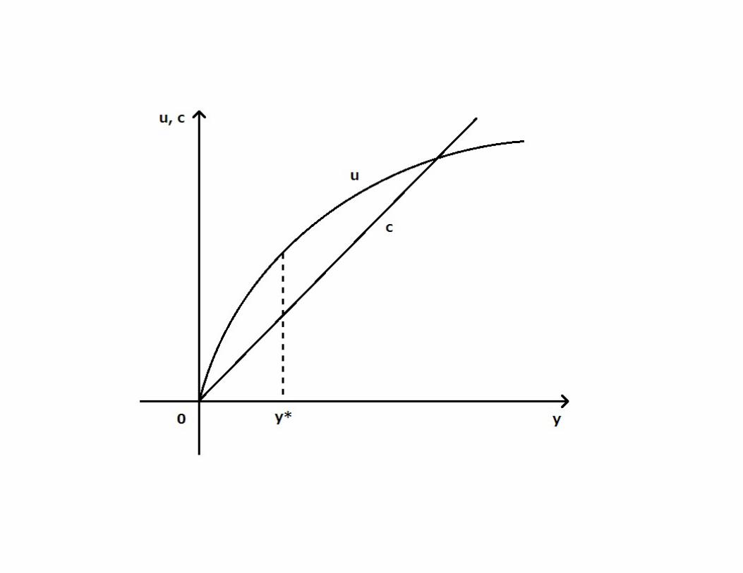
• period utility: consumer u(y); producer −c(y);
• no commitment: let y be maximum production under perfect moni-toring and let y∗ = argmax[u(y) − c(y)] > 0; perfect-monitoringoptimum is min{y, y∗} in every single-coincidence meeting
• no-monitoring

Extensions of Shi 1995 and Trejos-Wright 1995
• they studied the model with money holdings in {0, 1}
— the distribution of money is unaffected by trades
— there is no scope for transfers of money
• first two applications: abandon their limitation on asset holdings, butassume that asset holdings in meetings are common knowledge
• third application: keeps the {0, 1} restriction on asset holdings, butgeneralize the no-monitoring assumption
— some exogenous fraction of people are perfectly monitored and therest not at all (see Cavalcanti-Wallace 1999)

Ex ante optima from among implementable allocations
For each model, find the allocation that maximizes ex ante representative-agent discounted utility subject to two main restrictions:
• the allocation is a steady state
• the allocation is in the pairwise core for each meeting
Ex ante means before initial assets holdings are assigned and before type(monitored or not-monitored) is determined

Wataru Nozawa and Hoonsik Yang (unpublished, part of Yang’s 2016Ph.D. dissertation)
Consider Trejos-Wright 1995 with individual money holdings in {0, 1, 2, ..., B}and no explicit taxation
Sequence of actions:
• state of the economy is a distribution over {0, 1, 2, ..., B}, denoted π
• then pairwise meetings at random and trade with lotteries
• then (probabilistic ) transfers: non-negative and weakly increasing ina person’s money holding
• then inflation modeled as probabilistic iid loss δ (disintegration) ofeach unit of money held
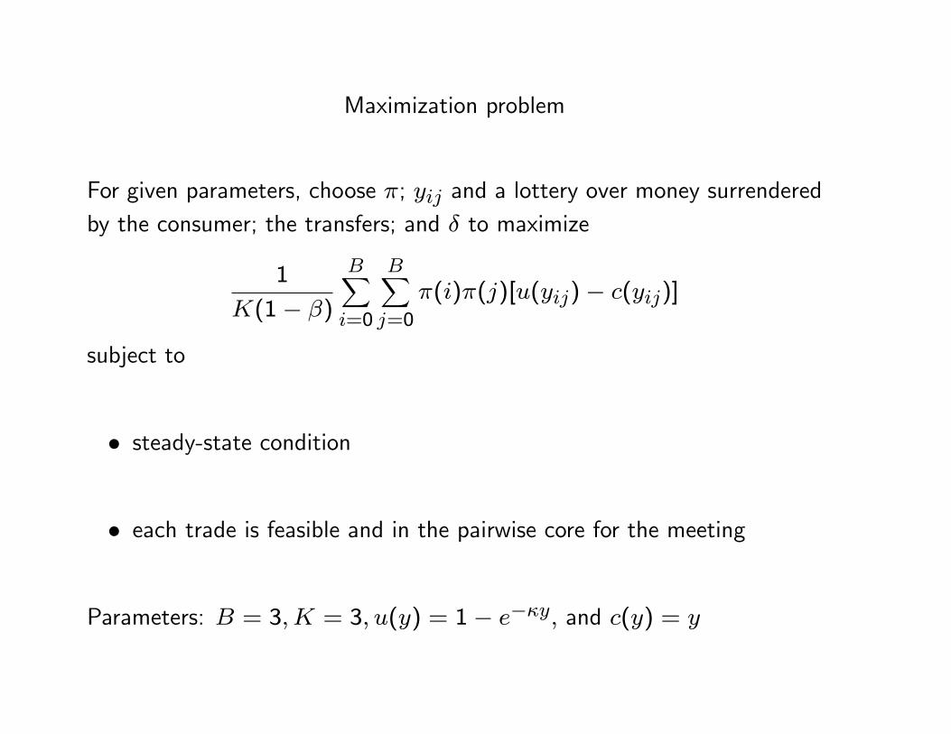
Maximization problem
For given parameters, choose π; yij and a lottery over money surrenderedby the consumer; the transfers; and δ to maximize
1
K(1− β)
B∑i=0
B∑j=0
π(i)π(j)[u(yij)− c(yij)]
subject to
• steady-state condition
• each trade is feasible and in the pairwise core for the meeting
Parameters: B = 3,K = 3, u(y) = 1− e−κy, and c(y) = y

Table 1. Optimal prob (%) of a unit transfer: the top number isfor those with 0 or 1, the bottom number is for those with 2
κ \ β .15 .2 .25 .3 .35 .4 .5 .6 .7 .8
2000
072
073
074
00
3.53.5
3.13.1
13.013.0
11.411.4
00
15 -00
065
067
067
00
00
5.35.3
2.82.8
00
12 - -00
059
061
00
00
2.12.1
00
00
10 - - -00
055
056
00
00
00
00
8 - - - -00
047
00
00
00
00
6 - - - - -00
038
00
00
00
5 - - - - - -00
00
00
00
4 - - - - - - -00.6
00
00
3 - - - - - - - -00.9
00
Lesson
Optimal policy is not simple
• even for this very simple model, the best policy is very dependent onthe parameters
The best policy ranges from paying substantial interest on large holdingsof money to giving lump-sum transfers– very different policies
• the former spreads out the distribution of money holdings, while thelatter compresses it

Coexistence of money and higher return assets
Hicks (1935): coexistence is the main challenge for monetary theory
• For Hicks, assuming a demand for money or putting money in theutility function are nonsenses
• Hicks proposed transaction costs (which we ought to regard as anothernonsense)
Cash-in-advance (CIA) did not exist when Hicks wrote
• Whether it gives rise to coexistence depends on your equilibrium notion

Individual defection or defection by the pair in each meeting
With individual defection, CIA is implementable
• each person choose from {yes, no} as response to a planner suggestedtrade
With defection by pairs, it, generally, is not
Tao Zhu and I (JET, 2007) took as our challenge getting coexistence whileallowing cooperative defection of the pair in each meeting

The partial equilibrium setting (strictly increasing and concavecontinuation value of nominal wealth)
Stage 1: portfolio choice
• government offers one-period discount bonds at a given price
• people with only money choose a portfolio
• (in the general equilibrium, interest is financed by money-creation)
Stage 2. Trejos-Wright (1995) with general portfolios of money and bonds

Stage-2 pairwise meetings
Bonds and money are perfect substitutes in terms of their payoffs at thestart of the next date
Therefore, pairwise-core outcomes are defined as a set of pairs: output ina meeting and the amount of wealth transferred
There are many pairwise-core outcomes: they range from giving all thegains-from-trade to the consumer to giving all to the producer
That allows us to reward buyers with a lot of money and, thereby, givespeople an incentive to leave stage-1 with some money

Comments
Role of pairwise trade (nondegenerate pairwise core)
Multiplicity (the favored assets could be money, bonds, or neither)
Welfare: can it be beneficial to have coexistence?
• Hu and Rocheteau (JET 2013)
— uses a version of Lagos-Wright (2005) with capital and money
— helps avoid over-accumulation of capital
• Hoonsik Yang (unpublished, part of his 2016 Ph.D. dissertation)
— works with examples in the Zhu-Wallace setting and the followingallowable portfolios: (0, 0), (1, 0), (2, 0) and (0, 1), (1, 1), (0, 2)
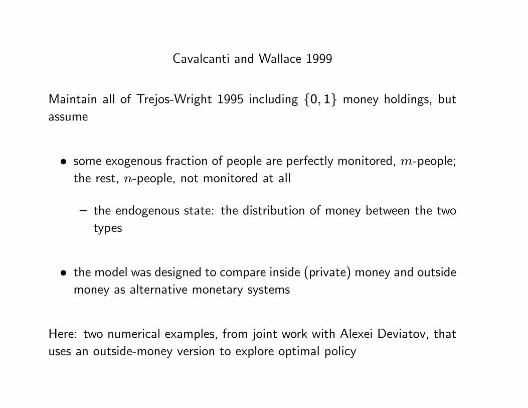
Cavalcanti and Wallace 1999
Maintain all of Trejos-Wright 1995 including {0, 1} money holdings, butassume
• some exogenous fraction of people are perfectly monitored, m-people;the rest, n-people, not monitored at all
— the endogenous state: the distribution of money between the twotypes
• the model was designed to compare inside (private) money and outsidemoney as alternative monetary systems
Here: two numerical examples, from joint work with Alexei Deviatov, thatuses an outside-money version to explore optimal policy

Monitoring and punishment
• ex ante identical people, but
— fraction α become permanently monitored (m-people)
— rest are permanently nonmonitored (n-people)
• for m-people, histories (and money holdings) are common knowledge
• for n-people, they are private
• monitored status and consumer/producer status are common knowl-edge
• only punishment is individual m→ n
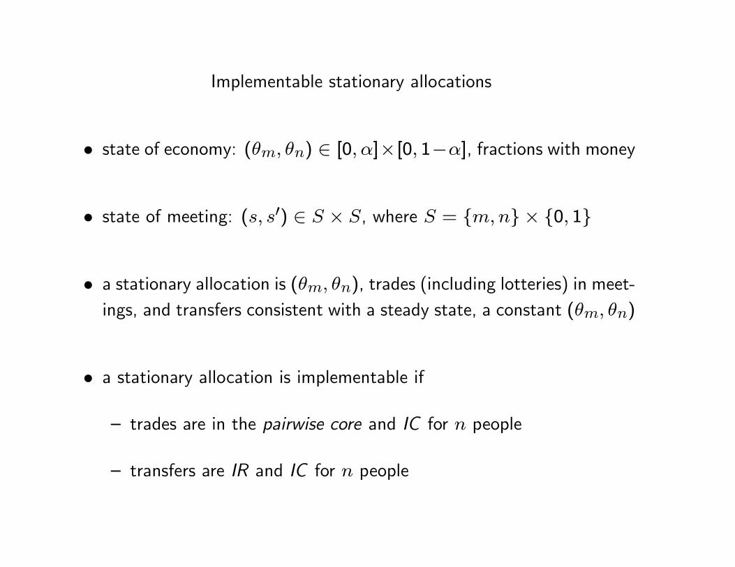
Implementable stationary allocations
• state of economy: (θm, θn) ∈ [0, α]×[0, 1−α], fractions with money
• state of meeting: (s, s′) ∈ S × S, where S = {m,n} × {0, 1}
• a stationary allocation is (θm, θn), trades (including lotteries) in meet-ings, and transfers consistent with a steady state, a constant (θm, θn)
• a stationary allocation is implementable if
— trades are in the pairwise core and IC for n people
— transfers are IR and IC for n people

The planner
Choose a stationary and implementable allocation to maximize ex anteexpected utility before initial s is realized for each person
• ex ante expected utility is proportional to∑s∈S
∑s′∈S
πsπs′[u(yss′)− c(yss′)]
where yss′ is output in the (s, s′) meeting and
(πm1, πm0, πn1, πn0) = (θm, α− θm, θn, 1− α− θn)
• first-best is proportional to u(y∗)−c(y∗), where y∗ = argmax[u(y)−c(y)]

Example 1: Optimal inflation (Deviatov and Wallace 2010; workingpaper)
• inflation: a person who ends trade with money loses it with someprobability
• parameters: u(y) = 1−e−10y, c(y) = y,K = 3, β = .59, α = 1/4;
— arbitrary except for β; high enough so that if α = 1, thenmin{y, y∗} =y∗; low enough so that if α = 0, then optimal (y, θn)� (y∗, 1/2),where y is output in trade meetings

The optimum
• welfare equal to 34% of first best
• all m-people start each date with money (θm = α)
• 24% of n-people start with money (θn = .24(1− α))
• 16% inflation rate
• transfers to m people, none to n people
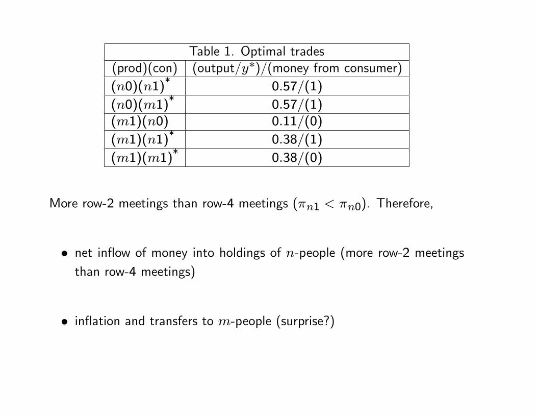
Table 1. Optimal trades(prod)(con) (output/y∗)/(money from consumer)(n0)(n1)* 0.57/(1)
(n0)(m1)* 0.57/(1)(m1)(n0) 0.11/(0)
(m1)(n1)* 0.38/(1)
(m1)(m1)* 0.38/(0)
More row-2 meetings than row-4 meetings (πn1 < πn0). Therefore,
• net inflow of money into holdings of n-people (more row-2 meetingsthan row-4 meetings)
• inflation and transfers to m-people (surprise?)
Similar inside-money result is in Deviatov and Wallace (RED 2014)
Inside money is different because money is issuer-specific
An m person defects without useful money
Transfers not needed, but the optimum has spending by m people thatexceeds earnings at each date, which produces inflation (surprise?)

Example 2. Optimal seasonal policy (Deviatov and Wallace JME 2009)
Same model except: a seasonal and zero average inflation is imposed
Parameters: α = 1/4, K = 3, u(y) = 2y1/2, β = .95, and
ct(y) =
{y/(0.80) if t is odd (winter)y/(1.25) if t is even (summer)
First date is odd (winter)
Implementable allocations: same except allowed to be two-date periodic
• If α = 1, then the first-best is implementable
• If α = 0, then the optimum is (yt, θnt) = (y∗t , 1/2) and welfare equalto 1/4 of first-best welfare

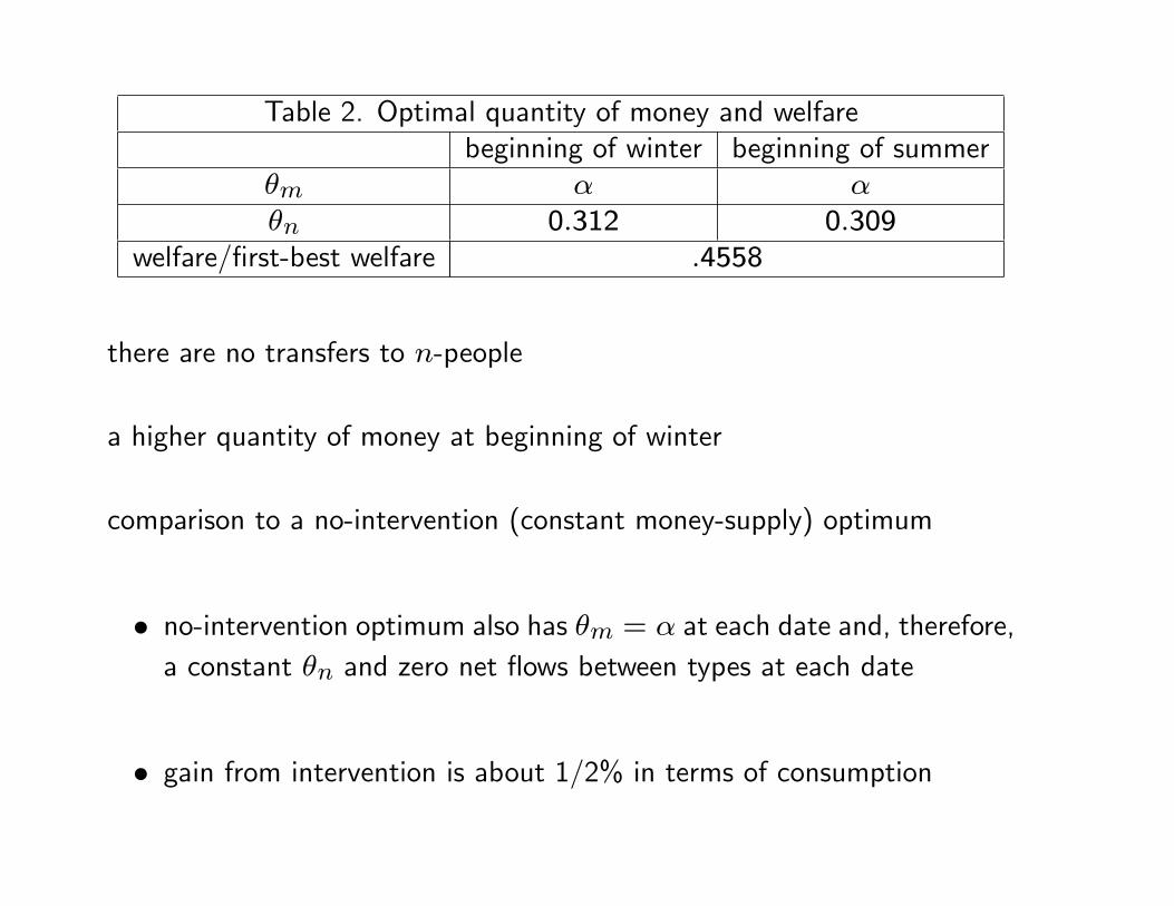
Table 2. Optimal quantity of money and welfarebeginning of winter beginning of summer
θm α αθn 0.312 0.309
welfare/first-best welfare .4558
there are no transfers to n-people
a higher quantity of money at beginning of winter
comparison to a no-intervention (constant money-supply) optimum
• no-intervention optimum also has θm = α at each date and, therefore,a constant θn and zero net flows between types at each date
• gain from intervention is about 1/2% in terms of consumption

Table 3. Optimal tradesmeeting (output/y∗t )/(money transferred)
(prod)(con) winter summer(n0)(n1) 0.95/(1.00) 0.95/(1.00)(n0)(m1) 0.85∗/(0.51) 0.78∗/(0.78)(m1)(n0) 0.16/(0) 0.17/(0)
(m1)(n1) 1.18†/(0.81) 0.84∗†/(1.00)(m1)(m1) 1.00/(0) 0.84∗/(0)
• net outflow from holdings of n people in winter, matching net inflowin summer
• m-people surrender money at beginning of summer and receive anexactly offsetting transfer at beginning of winter
— interpretation as planner loans: zero-interest loans to m-peopleat beginning of winter with repayment at beginning of summer(surprise and explanation?)
What can we learn from a few numerical examples?
They are consistent with the following related conclusions:
• if you know the model, then intervention is optimal
• even the qualitative nature of optimal intervention is not obvious
• optimal intervention depends on all the details
May need more examples to make those conclusions convincing
Concluding remarks
Somewhat standard view: judge a model not by the observations thatinspired it, but by its other implications that were not known when themodel was formulated. In that sense, the above applications are a tributeto the Shi and Trejos-Wright models.
Possible extensions:
• what if people in a meeting can hide assets
• nonstationary allocations and time consistent policy
• a large finite number of agents rather than a continuum