Models of Commodity Transfer - UCOP
55
UNIVERSITY OF CALIFORNIA DIVISION OF AGRICULTURAL. SCIENCES GIANNINI FOUNDATION OF AGRICULTURAL ECONOMICS Models of Con1modity Transfer Duran Bell, Jr. Giannini Foundation Monograph Number 20 • October, 1967 CALIFORNIA AGRICULTURAL EXPERIMENT STATION
Transcript of Models of Commodity Transfer - UCOP
UNIVERSITY OF CALIFORNIA DIVISION OF AGRICULTURAL. SCIENCES GIANNINI FOUNDATION OF AGRICULTURAL ECONOMICS
Models of Con1modity Transfer
Duran Bell, Jr.
Giannini Foundation Monograph Number 20 • October, 1967
CALIFORNIA AGRICULTURAL EXPERIMENT STATION

The purpose of this study was the development of mathematical models from which an industry, acting through a central decision unit, could determine each week the optimal quantity of its product to ship to the domestic market.
Interest in this topic has been stimulated by commodity transfer problems in the lemon industry. The lemon industry, which operates under a Federal Marketing Order, has desired for some time a means of increasing the effectiveness of its shipping policies in raising and stabliziog incomes of lemon growers. However, the task is made difficult by the existence of random and unanticipated short-run shifts in the level of demand (of wholesalers) for fresh lemons. lo this study these random elements were taken into account and the lemon transfer problem was examined as a stochastic process.
The monograph briefly discusses the lemon industry, a number of introductory transfer models and, then, focuses attention upon a class of stochastic models called "multi-stage." lo these models, "stages" are defined as disjoint and contiguous intervals of time in which certain kinds of decisions may be made with respect to the shipping quantity of a particular "period."
The multi-stage models are monopoly models of a peculiar sort: the firm is assumed to possess complete control over the marketing of the industry's product but no control over the level of production. It is further assumed that the firm seeks to minimize its expected net losses and that the demand function for its product is subject to short-run random disturbances. lo each successive stage of a shipping period, additional information about these disturbance terms becomes available and this information may be used to develop an "optimal" adjustment to an earlier shipping decision. The direction which the adjustment may take during any stage is predetermined and depends upon the "name" of that stage. Moreover, the unit cost of making an adjustment progressively increases from stage to stage. Hence, decisions made in earlier stages are made in the face of greater ignorance of demand but at lower unit costs of transfer.
The objective of a multi-stage model is to find, for each stage and for every element of the information set, a shipping policy which is optimal, optimal in the sense of posing a loss minimizing balance between the lower shipping cost and greater risk associated with early decisions and the higher shipping cost and smaller risk associated with later decisions.
THE AUTHOR:
Duran Bell, Jr., is Assistant Professor of Economics, University of California, Irvine. This study was developed by the author while on appointment as Research Assistant in the Department of Agricultural Economics, University of California, Berkeley.
Duran Bell, Jr.
Models of Commodity Transfer1
INTRODUCTION
The nature of mathematical models
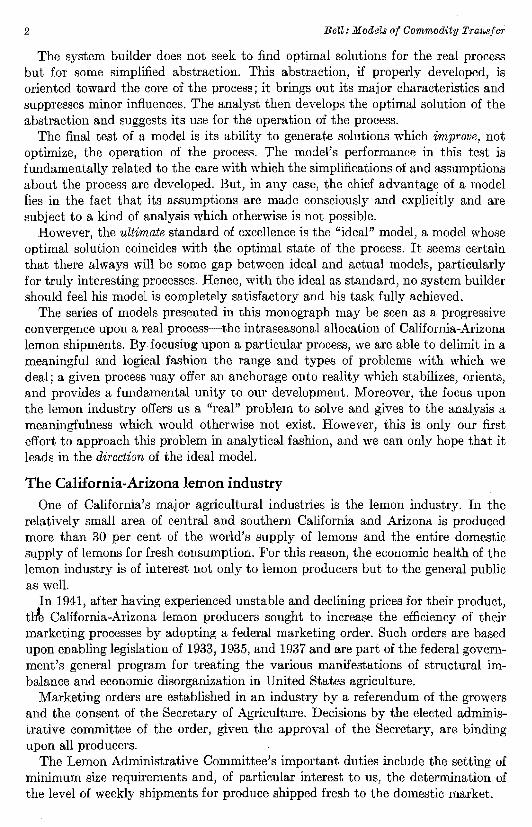
In recent years, a new field of study-"operational research"-is concerning itself with problems of making "optimal" decisions with respect to such practical business problems as determining proper levels of inventory, finding the best number of cashiers for a retail store, the best route for a delivery truck, and others. Although these problems have always found some sort of solution, it has been only in the past 20 years that they have been the focus of academic work. Mathematicians, mathematical economists, statisticians, industrial engineers, and "management experts" have joined in an effort to give a systematic treatment to a broad range of practical business and logistic problems.
Operations research is primarily oriented toward the optimization of "systems," theoretical abstractions, and simplifications of real processes. Within these systems, the technical and technological problems are generally assumed to be handled efficiently and the interest of the analyst is in developing a "system," or "model," from which he may discover ways of improving the operation of the process.
When management makes decisions, a great variety of factors may enter into its consideration and influence in some way its decisions, including its competitors, stockholders, self-pride, particular suppliers, and perhaps even the wife of the president. But the "system builder" who allows himself to succumb to such diverse considerations is doomed to defeat. He must seek to reduce the problem to its essential factors and preserve a reasonable relationship between them. In so doing, he hopes to be able to subject the problem to mathematically rigorous and logical analysis.
The ability of traditional management to recognize the many details of a process often leads to its undoing. Without a method of systematically simplifying the process, and without an analytical· procedure for dealing with selected factors, management often becomes overwhelmed by the complexities of a process, satisfied to "muddle through," to use "rules of thumb," or hunches. The result is that traditional management, while looking at a great many factors, actually nmy use very few of them in decision making and then may use them poorly.
1 Submitted for publication October 21, 1966.
In this publication, for technical reasons, superscripts and subscripts in mathematical formulas are sometimes printed next to each other instead of on top of each other. For instance:
ea* is used instead of e:; or S(f) H is used instead of S~-i'
[ l J
2 Bell: Models of Commodity Transfer
The system builder does not seek to find optimal solutions for the real process but for some simplified abstraction. This abstraction, if properly developed, is oriented toward the core of the process; it brings out its major characteristics and suppresses minor influences. The analyst then develops the optimal solution of the abstraction and suggests its use for the operation of the process.
The final test of a model is its ability to generate solutions which improve, not optimize, the operation of the process. The model's performance in this test is fundamentally related to the care with which the simplifications of and assumptions about the process are developed. But, in any case, the chief advantage of a model Hes in the fact that its assumptions are made consciously and explicitly and are subject to a kind of analysis which otherwise is not possible.
However, the ultimate standard of excellence is the "ideal" model, a model whose optimal solution coincides with the optimal state of the process. It seems certain that there always will be some gap between ideal and actual models, particularly for truly interesting processes. Hence, with the ideal as standard, no system builder should feel his model is completely satisfactory and his task fully achieved.
The series of models presented in this monograph may be seen as a progressive convergence upon a real process-the intraseasonal allocation of California-Arizona lemon shipments. By focusing upon a particular process, we are able to delimit in a meaningful and logical fashion the range and types of problems with which we deal; a given process may offer an anchorage onto reality which stabilizes, orients, and provides a fundamental unity to our development. Moreover, the focus upon the lemon industry offers us a "real" problem to solve and gives to the analysis a meaningfulness which would otherwise not exist. However, this is only our first effort to approach this problem in analytical fashion, and we can only hope that it leads in the direction of the ideal model.
The California-Arizona lemon industry One of California's major agricultural industries is the lemon industry. In the
relatively small area of central and southern California and Arizona is produced more than 30 per cent of the world's supply of lemons and the entire domestic supply of lemons for fresh consumption. For this reason, the economic health of the lemon industry is of interest not only to lemon producers but to the general public as well.
In 1941, after having experienced unstable and declining prices for their product, tl:!e California-Arizona lemon producers sought to increase the efficiency of their marketing processes by adopting a federal marketing order. Such orders are based upon enabling legislation of 1933, 1935, and 1937 and are part of the federal government's general program for treating the various manifestations of structural imbalance and economic disorganization in United States agriculture.
Marketing orders are established in an industry by a referendum of the growers and the consent of the Secretary of Agriculture. Decisions by the elected administrative committee of the order, given the approval of the Secretary, are binding upon all producers.
The Lemon Administrative Committee's important duties include the setting of minimum size requirements and, of particular interest to us, the determination of the level of weekly shipments for produce shipped fresh to the domestic market.
3 MONOGRAPH • No. 20 • October, 1967
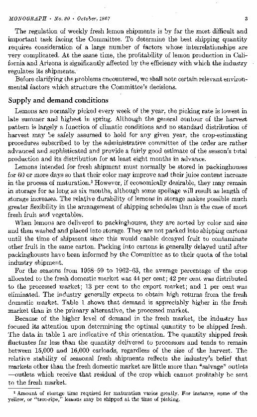
The regulation of weekly fresh lemon shipments is by far the most difficult and important task facing the Committee. To determine the best shipping quantity requires consideration of a large number of factors whose interrelationships are very complicated. At the same time, the profitability of lemon production in California and Arizona is significantly affected by the efficiency with which the industry regulates its shipments.
Before clarifying the problems encountered, we shall note certain relevant environmental factors which structure the Committee's decisions.
Supply and demand conditions
Lemons are normally picked every week of the year, the picking rate is lowest in late summer and highest in spring. Although the general contour of the harvest pattern is largely a function of climatic conditions and no standard distribution of harvest may be safely assumed to hold for any given year, the crop-estimating procedures subscribed to by the administrative committee of the order are rather advanced and sophisticated and provide a fairly good estimate of the season's total production and its distribution for at least eight months in advance.
Lemons intended for fresh shipment must normally be stored in packinghouses for 60 or more days so that their color may improve and their juice content increase in the process of maturation.2 However, if economically desirable, they may remain in storage for as long as six months, although some spoilage will result as length of storage increases. The relative durability of lemons in storage makes possible much greater :flexibility in the arrangement of shipping schedules than is the case of most fresh fruit and vegetables.
When lemons are delivered to packinghouses, they are sorted by color and size and then washed and placed into storage. They are not packed into shipping cartons until the time of shipment since this would enable decayed fruit to contaminate other fruit in the same carton. Packing into cartons is generally delayed until after packinghouses have been informed by the Committee as to their quota of the total industry shipment.
For the seasons from 1958-59 to 1962-63, the average percentage of the crop allocated to the fresh domestic market was 44 per cent; 42 per cent was distributed to the processed market; 13 per cent to the export market; and 1 per cent was eliminated. The industry generally expects to obtain high returns from the fresh domestic market. Table 1 shows that demand is appreciably higher in the fresh market than in the primary alternative, the processed market.
Because of the higher level of demand in the fresh market, the industry has focused its attention upon determining the optimal quantity to be shipped fresh. The data in table 1 are indicative of this orientation. The quantity shipped fresh :fluctuates far less than the quantity delivered to processors and tends to· remain between 15,000 and 16,000 carloads, regardless of the size of the harvest. The relative stability of seasonal fresh shipments reflects the industry's belief that markets other than the fresh domestic market are little more than "salvage" outlets -outlets which receive that residual of the crop which cannot profitably be sent to the fresh market.
2 Amount of storage time required for maturation varies greatly. For instance, some of the yellow, or "tree-ripe," lemons may be shipped at the time of picking.

4 Bell: Models of Commo!Uty Tranisfer
TABLE 1
ON-TREE PRICES AND CARLOADS SHIPPED OF FRESH AND PROCESSED LEMONS: CALIFORNIA, 195~56 TO 1962---63
Season Ou-tree price
F""'h
Shipped
! Processed
On-tree price Shipped
dollars per packed equivalent box carloads dollars per packer' carloadsequivalent baz
1955-56. . . . . . . . . . . . . . . . . . .. .. . . . 1956--57. .. .. . . . .. .. . . . . .. . . . . . . . . 1957-58....................... 1958-59..... .... . ... . . . . . .... . .. . 1959-IJO........ . . . .. .. . . . . . . . . . 1960-61.......................... 1961-62...... ... .. .. . .. . . . . . . . . . . . 1962-63 .. . . .. . . . . . . . . .. .. . . . .. . ..
3. 28 2 .45 2.24 2.64 2.53 2.34 2.49 3 . 60
16,041 15,978 15,352 15,598 15,063 15,025 15, 258
0.38 8,906 0.12 13,390 0.20 H,332
-0.38• 18,782 -0.32• 18,517
0.14 9,572 0.08 16, 064 0.28
l •The appearance of negative prices results from the fact that on-tree prices are roughly equivalent to f.o.b. prices
minus unit costs of picking, packing, and hauling~ SOURCES:
Cols. 1 and 3: Sunkist Growers, 1964 Supplement, Btatistir.al Information on the Citrus Fruit Industry (Los Angeles, 1964), p. 19.
Cols. 2 and 4: Lemon Administrative Committee, Annual Report (Los Angeles, 1961··1963), p. 8.
The merits of treating the nonfresh domestic markets as salvage outlets were examined by Hoos and Kuznets (1962) and, earlier, by Hoos and Seltzer (1952), who showed through statistical analysis that the quantity shipped to processors may exert a strong influence upon the seasonal average price in the fresh market. This evidence indicates that the industry should determine an optimal balance between fresh and processed utilization.
The study (Hoos and Kuznets, 1962) utilized the methods of multiple regression analysis and was based upon available time series data. Its objective was to explain variations in seasonal average prices and, presumably, the results could be useful in aiding the lemon industry to determine the percentage of the crop which should be allocated to the fresh market. But analyses based upon seasonal or monthly data do not provide the information which is necessary for the efficient allocation of the seasonal fresh shipment quota (however determined) among the many weeks of the season. 'Yet, these studies do indicate two factors which one may expect to hold in the
case of weekly price variations: (1) that demand for fresh lemons is inelastic within the range of prevailing prices and (2) that average daily temperature during the spring and summer months exerts a strong positive influence on the level of demand.
The inelasticity of demand implies that prices are relatively sensitive to changes in the quantity of lemons sold and that the total revenue to growers from the sale of some quantity decreases with the increase in that quantity. The consequence is that the economic profitability of lemon sales is sensitive to "errors" in the determination of the quantity to be shipi:;ed.
On the other hand, the importance of temperature implies that errors will be made more frequently because current methods of forecasting temperature lead frequently to predicted temperatures which vary widely from the actual.
5 MONOGRAPH • No. 20 • October, 1967
The existence of these two factors, then, requires that the determination of shipments be done carefully and with due regard for the risks which result from incomplete information with respect to demand.
The "Objective Function" and procedure of the Committee
According to the Committee's marketing policy for the 1963---04 lemon crop, dated November 13, 1963, " ... it shall be the policy of the Committee to recommend the shipment of the maximum quantity of lemons in the fresh fruit market that can be sold at prices which will return the highest possible overall return within the parity provision of the Agricultural Marketing Agreement Act of 1937, as amended, consistent with the best interests of the industry."
This statement of policy, in spite of an apparent internal contradiction, appears to establish profit maximization as the Committee's objective. But, apparently, its effort to act upon this criterion tends to be confined to its decisions with respect to the overall allocation of the season's production.
OncP- the Committee has established the quantity to be shipped fresh, it has maintained a practice of scheduling weekly shipments in such a way that (1) prices will be maintained at an "acceptable" level and (2) the weekly shipments will, in aggregate, approximate the previously determined seasonal objective. 3
In actual practice, this weekly allocation policy approaches, or implies, an objective which might be described as "maximizing output under a price constraint." However, it appears that their use of this policy, or objective function, on a weekly basis is imposed upon them by the difficulty of implementing the more desirable objective of maximizing returns to growers (given the season's quantity goal).
The intraseasonal objective function presently used in the lemon industry is one which is easier to make operational by rules-of-thumb than is the maximization criterion. And it may be impossible to seek revenue maximization as a goal in the absence of an explicit analytical procedure for determining the shipping quantities.
The administrative procedure
To enable the various sales organizations to consummate order agreements with buyers, the Committee always announces a preliminary (maximal) industry shipping quantity one week in advance. Then, on Tuesday of the week of shipment, at which time the Committee normally meets, the Committee is free to recommend an increase in that quantity by any positive amount in view of hitherto unavailable information with respect to current supply and/or demand conditions. 4
The nonnegativity of this last-minute adjustment is based upon the fact that the sale of much of the fruit is arranged by contract during the week prior to the week of shipment; moreover, many downward adjustments would create administrative and other problems for the packinghouses."
a The seasonal goal is not fixed and rigid throughout the season but is subject to reevaluation and alteration during the year.
4 Actually, the Committee is able to increase the maximal shipping quantity at any time prior to (approximately) ll :00 a.m. on Thursday of the effective week. This time restriction results from the requirement that the industry's decision be recorded in the Federal Register.
6 The Committee merely sets maximal levels of shipment for each shipper, and shippers may, individually, elect to ship less than their maximum. Their actual shipment, however, i:s generally close to the Committee's quota.
6 Bell: ModrJls of Commodity Transfer
However, even during the week of the shipment, the demand conditions that the shipped fruit will face are quite uncertain. About 50 per cent of the fresh carloads are sent to Chicago and New England and transit time for such shipments, if made direct, is about six or seven days; shipments to Dallas or Seattle, on the other hand, require much less time. For all geographical areas, the quantity weighted average transit time is about five days. Moreover, shipments of a given week may depart on any day of that week. This means that the Committee must anticipate demand conditions for about two weeks in advance at the time that the initial shipping quantity is determined and about one week in advance when a possible upward adjustment in that quantity is considered. Hence, it could hardly be expected that the Committee would be able to determine shipments without making mistakes.
The objective and framework of this study With the lemon transfer problem as our principal focus, we shall attempt to pro
gress from a class of simple, deterministic transfer models to a class of stochastic sequential decision models. Our ultimate objective is the development of a theoretical model of the lemon transfer problem which is capable of incorporating efficiently most of the relevant quantifiable information which the Committee possesses, or is able to possess, .at the time it makes its decisions. The discussion, however, is general and the significance of the model is in no way restricted to a particular industry.
We begin with .a number of introductory transfer models. The value of presenting these models is twofold: (1) It enables us to introduce various aspects of transfer problems, both gradually and clearly, and (2) it will help clarify the place of the "multistage" models within a general class of problems.
Then, we develop and discuss sequential decision multistage models. Our objective is to find optimal solutions to problems in which it is possible for a firm to be flexible with respect to transfer decisions, that is, when the firm is able to alter its decisions given better information with respect to supply and/or demand conditions.
Introductory Models
At present, almost no literature on shipping models per se exists. Almost all of the work which relates to shipping problems has been oriented toward "inventory" processes in which the shipping problem is analyzed from the receiver's, not the silnder's, point of view. It is likely that this neglect of shipping models results in large part from the fact that the firms which the researchers wish to serve usually pursue manufacturing operations and wholesale or retail trade. In most of these situations, it may safely be assumed that the selling price of the commodity in question is fixed and known with certainty, and that most shipments are made in response to orders from customers. Seldom does the manufacturer or the wholesaler need to be concerned with the rate of shipment as a decision variable because this rate is exogenously determined (for the :fixed price); his concern is more likely to rest with the determination of the optimal level of inventory from which this .demand is satisfied.
For most agricultural commodities, however, the fresh-product price is not
7 MONOGRAPH • No. 20 • October, 1gfJ7
administratively fixed; and any agency that seeks to direct the shipping policy for the industry must face a demand curve-a relation between price and quantitynot simply an exogenous rate of demand. Moreover, only a fraction of the quantity shipped is likely to be in response to direct orders from buyers. Hence, the rate of product exit from inventory becomes a crucial decision variable.
Although the absence of administratively fixed prices in agriculture precludes the direct and effective use of most inventory models for agricultural shipping processes, inventory models are concerned with many of the same variables and with similar cost factors. For this reason, there is much we may learn about shipping systems through the analysis of inventory systems. 6
The nature of transfer systems
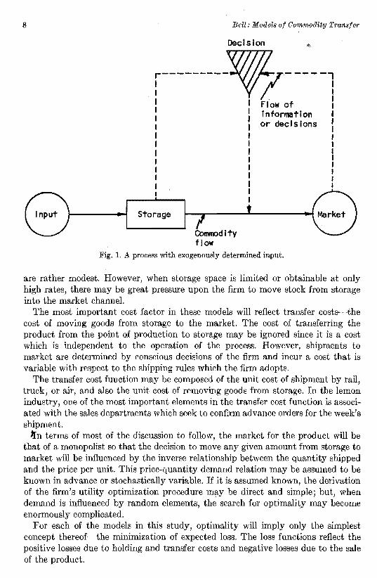
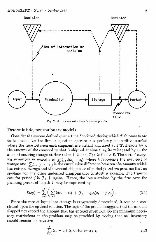
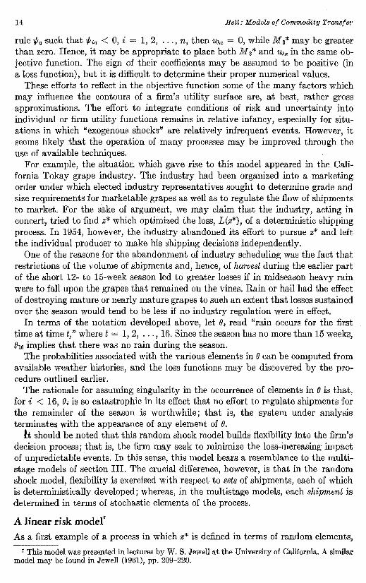
The transfer systems to·be considered in this study possess only one decision variable, the rate of product exit from inventory; and it is assumed that the objective of the firm is to minimize the (expected) value of its net financial loss where both the levels of consumer demand and the rate of product entry into inventory are exogenously determined. A picture of such a system is provided by figure 1.
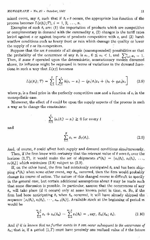
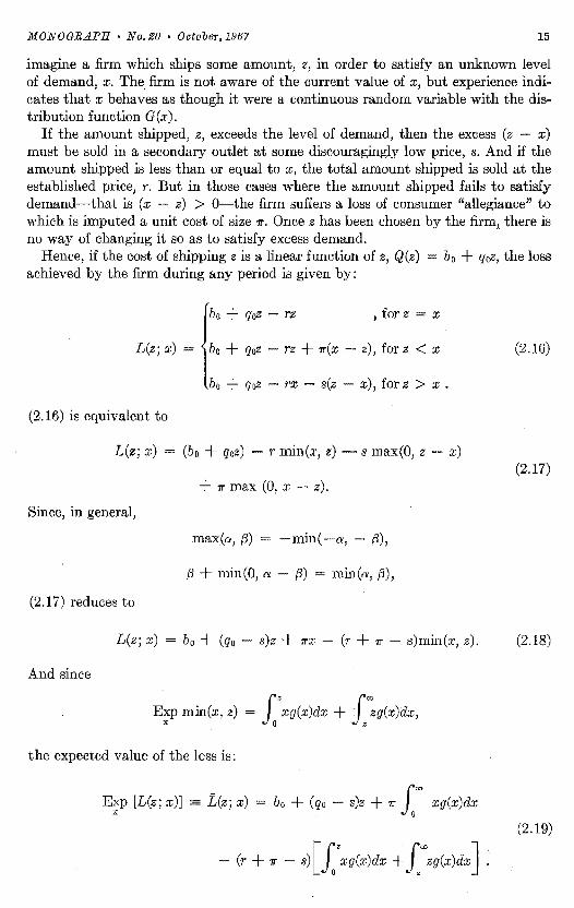
A system which may be encountered more often is shown in figure 2. In this case, the rate of flow into storage is determined by a production decision so that the process has two decision points. This kind of process is typical of manufacturing operations. Frequently, a manufacturing firm contains many points of storage for separate components of a product or for a given component at various stages of completion. The analysis of this process, however, may be impossible if both decision points are attacked simultaneously. A feasible approach is the following: Isolate that part of the system which contains the transfer process and find for all possible rates of production the best rate of shipment, i.e., treat the rate of production as an exogenous variable; then, find the best rate of production, given the corresponding optimal shipping rules. This reduces the total process to two subprocesses, one of which is the focus of this study.
So, we may state more correctly that the rate of input into storage is exogenous to the system under investigation but not necessarily independent of decisions by the firm.
Once produced, the product will be assumed to move immediately into storage. There are many possible characteristics of the storage facility which could be recognized: limited storage space, stochastically variable storage capacity, a multitude of storage units at various distances from the source of production or with distinctly different charges per unit of storage, situations where some of the product may bypass storage altogether, etc.
Although certain capacity limitations will be introduced into some of the models of this chapter, the storage unit will generally be undefined in both dimension and space. The central characteristic of storage, for our purpose, will be the unit cost per period to the shipping firm of holding the product in storage.
The factors which enter into the determination of the cost of holding may include not only the rental price of storage space but also costs because of spoilage, pilferage, taxation, insurance, etc. In the case of the lemon industry, variable storage costs
6 For a good introduction to inventory analysis, see Hadley and Whitin (1963).
8 Bell: Models of Commodity Transfer
Decision
r---------~- --- -: ' IFlow of 1
Information I or decisions I
I I I I I I I I
Storage
Commodity flow
Fig. 1. A process with exogenously determined input.
are rather modest. However, when storage space is limited or obtainable at only high rates, there may be great pressure upon the firm to move stock from storage into the market channel.
The most important cost factor in these models will reflect transfer costs·-the cost of moving goods from storage to the market. The cost of transferring the product from the point of production to storage may be ignored since it is a cost which is independent to the operation of the process. However, shipments to market are determined by conscious decisions of the firm and incur a cost that is variable with respect to the shipping rules which the firm adopts.
The transfer cost function may be composed of the unit cost of shipment by rail, truck, or air, and also the unit cost of removing goods from storage. In the lemon industry, one of the most important elements in the transfer cost function is associated with the sales departments which seek to confirm advance orders for the week's shipment.
JJ:n terms of most of the discussion to follow, the market for the product will be that of a monopolist so that the decision to move any given amount from storage to market will be influenced by the inverse relationship between the quantity shipped and the price per unit. This price-quantity demand relation may be assumed to be known in advance or stochastically variable. If it is assumed known, the derivation of the firm's utility optimization procedure may be direct and simple; but, when demand is influenced by random elements, the search for optimality may become enormously complicated.
For each of the models in this study, optimality will imply only the simplest concept thereof-the minimization of expected loss. The loss functions reflect the positive losses due to holding and transfer costs and negative losses due to the sale of the product.
9 MONOGRAPH • No. 20 • October, 196'1
Decision Decision
w-------------------\. /v-, :low of Information or 'y'
decision T : I / I
I I I I I I I
Production Storage
Comrrodity flow
Fig. 2. A process with two decision points.
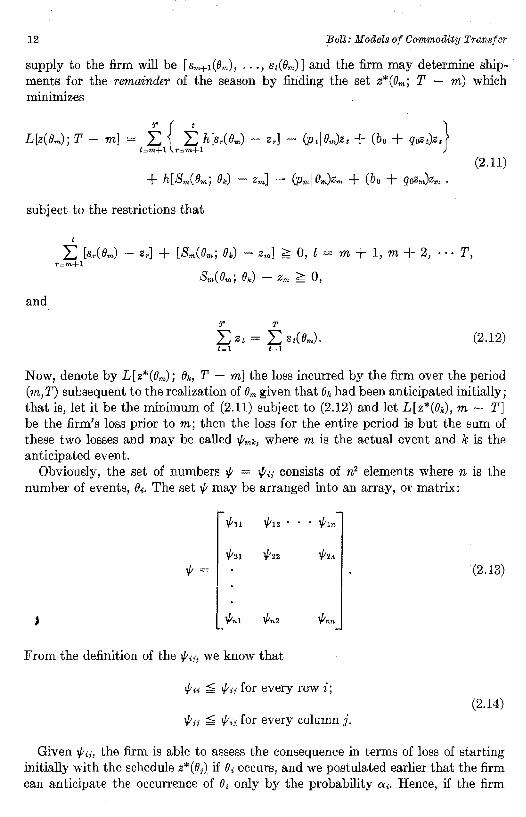
Deterministic, nonstationary models
Consider the system defined over a time "horizon" during which T shipments are to be made. Let the firm in question operate in a perfectly competitive market where the time between each shipment is constant and fixed at 1/T. Denote by Zt the amount of the commodity that is shipped at time t; Pt, its price; and by St, the amount entering storage at time t; t = 1, 2, · · ·, T; z ~ O; s > 0. The cost of carrying inventory in period j is .L:L 1 h(st - Zt), where h represents the unit cost of storage and .L:L (st - Zt) is the cumulative difference between the amount which has entered storage and the amount shipped as of period j; and we presume that no spoilage nor any other undesired disappearance of stock is possible. The transfer cost for period j is (bo + q0zf)Zf . Hence, the loss sustained by the firm over the planning period of length T may be expressed by
L(z;t) = ~ ( t h(sr - Zr) + (bo + qiizt)Zt - P~t) . (2.1)
Since the rate of input into storage is exogenously determined, it acts as a constraint upon the optimal solution. The logic of the problem suggests that the amount shipped not exceed the amount that has entered inventory. So the minimum necessary restrictions on the problem may be provided by stating that net inventory should remain nonnegative
L t
(sr - Zr) ~ 0, for every t, (2.2) r~l

10 Bell: Models of Commodity Transfe1·
and that the season's supply, S, be sold
.T T
LZt = L St= s. (2.3) t-1 t- 1
Expansion of (2.1) yields
T
L(z;t) = L [h(1' + 1 - t)(si - Zi) + (bo + qoZt)Zi - PtZi] (2.4) t-1
which, upon eliminating the s1 as exogenously determined, reduces to
T
G(z;t) = L [qoZ~ + (bo Pt)Zt - h(T + 1 - t)Zi] . (2.5) t-1
G(z;t) is a rather simple quadratic objective function, subject to linear constraints, the minimum of which may be easily determined by available techniques.
Now, suppose that the commodity, z, were perishable in storage so that any item which remains in storage for a duration longer thank may be assumed to be decayed and of no economic value, then it would be desirable to add an additional restriction which has the effect of precluding the shipment of decayed goods. Such a restriction may be satisfied if we require that
j j
L (st - z1) ;;£ L St, for j k + I, k + 2, · · · , T, t-1 j-k+l
or equivalently
j-k j
L St;;£ L Zt. (2.6) !- l l-1
Within the linear and nonlinear programming framework, we are free to alter not only the constraints but the objective function as well. Consider the case of a marketing monopoly, such as an agricultural marketing order, where the level of production and the rate of input into storage are exogenously determined and the deJJ.and curve facing the firm is given by
Pt = a - /3Zt + 'YYt , with f3 > 0 and Yt is any time dependent variable. Then, the variable loss function, G(z ;t), corresponding to (2.5) becomes
G(z ;t) = f, {z~(!3 + qo) Zt[(cx + 'YYD + h(T + 1) - (ht+ bo)]} (2.7) t-1 ...
Deterministic systems under random exogenous shock
Suppose that some multiperiodic shipping system, viewed as a deterministic process, operates under the threat or promise of some strong exogenously deter
11 MONOGRAPH • No. 20 • Ootober, 1967
mined event, say e, such that if (Ji E () occurs, the appropriate loss function of the process becomes L(z(e;) ;T), i = 1, 2, ... , n.
Examples of such (Ji are: (1) the importation of products which are competitive or complementary in demand with the commodity z, (2) changes in the tariff rates levied against z or against imports of products competitive with z, and (3) harsh weather conditions such as heavy frost or rain which damage the quality or lower the supply of z or its competitors.
Suppose that the set () consists of all simple (uncompounded) possibilities so that the probablity of the occurrence of any e, is a;, 0 ~ ai < 1, and .L:1= 1 a; 1. Then, if some () operated upon the deterministic, nonstationary models discussed above, its influence might be expressed in terms of variations in the demand functions in such a way that L(z ;t) becomes
T [ t L(z(e,); T) = ~ ,~ h(sr (2.8)
where p 1 is a fixed price in the perfectly comi;etitive case and a function of Zt in the monopolistic case.
Moreover, the effect of () could be upon the supply aspects of the process in such a way as to change the constraints:
t
L (sr(e,) - Zr) ~ 0 for every t '=l
and
T
L Zt = Sr(O;). (2.9) . t-1
And, of course, e could affect both supply and demand conditions simultaneously. Then, if the firm knew with certainty that the relevant value of Owere ek over the
horizon (1,T), it would make the set of shipments z*(ek) [z 1(8k), z2(ek), •.. , Z1·(81r)] which minimizes (2.8) subject to (2.9).
If, on the other hand, the firm had mistakenly anticipated ()k and has been shipping z*(Bk) when some other event, say Om, occurred, then the firm would probably change its course of action. The nature of this changed course is difficult to specify in the general case, but certain additional assumptions about () may be made such that some discussion is possible. In particular, assume that the occurrences of any Om will take place (if it occurs) only at some known point in time, m. So, if the firm had been anticipating ()k when Om occurred, it will have already shipped the sequence [z1(0k), z2(ek), · · ·, Zm-1(8k)]. Available stock at the beginning of period m would be
m-1 m-1
L St +Sm( Om) - L Zi(Bk) = , say, Sm(Omj ek). (2.10) t= 1 t= 1
And if it is known that no further events in () can occur subsequent to the occurrence of em; that is, if a period (1,T) must have precisely one realized value of() the future
12 Bell: Models of Commodity Transfer
supply to the firm will be [Sm+1(0m), ... , s1(e,,,)] and the firm may determine ship-· ments for the remainder of the season by finding the set z*(em; T - m) which minimizes
(2.11)
subject to the restrictions that
t
L [sr(Om) - Zr] + [Sm( Om; Oi.) Zm] ;;; 0, t = m + 1, m + 2, · · · T, T=m+I
and
T T
L Zt = L 8t(Om)• (2.12) 1-1 t~l
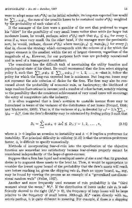
Now, denote by L[z*(O,,,); ek, T - m] the loss incurred by the firm over the period (m, T) subsequent to the realization of em given that ek had been anticipated initially; that is, let it be the minimum of (2.11) subject to (2.12) and let L[z*(ek), m - T] be the firm's loss prior to m; then the loss for the entire period is but the sum of these two losses and may be called 1/lmk, where m is the actual event and k is thr. anticipated event.
Obviously, the set of numbers if; if;.;; consists of n2 elements where n is the number of events, e._ The set if; may be arranged into an array, or matrix:
1/112 • 1/11n,~,, 1/121 1/122 1/1211
iJ; = . (2.13)
, l;., 1/ln2 1/lrm
From the definition of the 1/l;i, we know that
1/;u, ~ 1/l;i for every row i; (2.14)
1/lii ~ 1/;;; for every column j.
Given 1/;;;, the firm is able to assess the consequence in terms of loss of starting initially with the schedule z*(ei) if O; occurs, and we postulated earlier that the firm can anticipate the occurrence of O; only by the probability a;. Hence, if the firm
13 MONOGRAPH • No. 20 • October, 1967
were to adopt some set z*(lh) as its initial schedule, its long-run expected loss would be .L:~~ 1 aii{;;k, the sum of the possible losses to be sustained under z*(Bk) weighted by the probability of each value of 8.
If the manager of the firm were a gambler of the sort that preferred to wager his "shirt" for the possibility of very small losses rather than settle for larger but moderate losses, he would, perhaps, select z*(8 0 ) such that i/;00 ;;;;; l/;;>, for every i, even if a 0 were very small. On the other hand, if the manager were the pessimistic sort, he would, perhaps, choose z*(8p) where max;(i/;;, p) ;;;;; max;(l/;;, 3) for every j; that is, choose the strategy which corresponds with the column of l/; for which the largest element is the smallest within the set of largest elements, regardless of the magnitude of ap. However, for our purposes both men are probably nonrational and in need of a management consultant.
The consultant has the difficult task of ascertaining the utility function and psychological state of his client. He could recommend that the firm select shipping policy k, such that L~~ 1a;l/J;k ;;;;; L~= 1 a;l/J;ii j = 1, 2, ... , n-that is, follow the policy for which the long-run expected loss is minimum. But long-run losses may not represent the sole criterion of choice for the firm. The firm may also be concerned about the probability of economic ruin, or bankruptcy; the likelihood of large random fluctuations in income; and a number of other factors, notably relating to the possibility that the consistent achievement of very small losses will encourage the entry of competitors into the industry.
It is often suggested that a firm's aversion to unstable income flows may be formulated in terms of the variance of the distribution of net losses (Freund, 1956; and Markowitz, 1960). That is, if the variance of l/J;k is denoted by uk2 = l/n .L:'L1 •
(l/lik if/k)2, then the firm's disutility may be minimized by finding policy k such that
" D1c = L a11/lik + l1u~ ;;;;; Dh j 1, 2, ... , n, (2.15)
i=l
where A > 0 implies an aversion to instability and A < 0 implies a preference for instability. The principal difficulty in utilizing (2.15) is that the aversion-preference factor, A, is difficult to specify numerically.
Methods of incorporating fear-of-ruin into the specification of the objective function are somewhat less satisfactory because fear-of-ruin properly cannot be considered independently of the hope-of-great-success.
Suppose that a firm has liquid and semiliquid assets of size a and that its grandest desire is to augment these assets to the level A.a. Then, it would be appropriate to consider the lowest upper bound of the probability that the firm's assets will reach zero before reaching A.a, given the shipping rule i/;i.. Such an upper bound, U?.a, say, may be found by viewing the process as an example of a "generalized one-dimensional random walk" (Feller, 1957).
Another and more frequently used measure of ruin probability is the "third moment about the mean," JJ!fs*. If the distribution of losses under rule l/Jk is sufficiently skewed to the right (Ms* > O), the frequency of large losses will be large relative to the frequency of small losses. Although Ms* varies directly with UAa,
ceteris paribus, it is quite different in meaning. For example, if there is a shipping
14 Bel!: Models of ComrtWdity Transfer
rule if;q such that fiq < 0, i 1, 2, ... , n, then uxa = 0, while M3* may .be greater than zero. Hence, it may be appropriate to place both M 3 * and u~a in the same objective function. The sign of their coefficients may be assumed to be positive (in a loss function), but it is difficult to determine their proper numerical values.
These efforts to reflect in the objective function some of the many factors which may influence the contours of a firm's utility surface are, at best, rather gross approximations. The effort to integrate conditions of risk and uncertainty into individual or firm utility functions remains in relative infancy, especially for situations in which "exogenous shocks" are relatively infrequent events. However, it seems likely that the operation of many processes may be improved through the use of available techniques.
For example, the situation which gave rise to this model appeared in the California Tokay grape industry. The industry had been organized into a marketing order under which elected industry representatives sought to determine grade and size requirements for marketable grapes as well as to regulate the flow of shipments to market. For the sake of argument, we may claim that the industry, acting in concert, tried to find z* which optimized the loss, L(z*), of a deterministic shipping process. In 1954, however, the industry abandoned its effort to pursue z* and left the individual producer to make his shipping decisions independently.
One of the reasons for the abandonment of industry scheduling was the fact that restrictions of the volume of shipments and, hence, of harvest during the earlier part of the short 12- to 15-week season led to greater losses if in midseason heavy rain were to fall upon the grapes that remained on the vines. Rain or hail had the effect of destroying mature or nearly mature grapes to such an extent that losses sustained over the season would tend to be less if no industry regulation were in effect.
In terms of the notation developed above, let e1 read "rain occurs for the first time at time t," where t 1, 2, ... , 16. Since the season has no more than 15 weeks, 016 implies that there was no rain during the season.
The probabilities associated with the various elements in ecan be computed from available weather histories, and the loss functions may be discovered by the procedure outlined earlier.
The rationale for assuming singularity in the occurrence of elements in e is that, for i < 16, o, is so catastrophic in its effect that no effort to regulate shipments for the remainder of the season is worthwhile; that is, the system under analysis terminates with the appearance of any element of 8.
it should be noted that this random shock model builds flexibility into the firm's decision process; that is, the firm may seek to minimize the loss-increasing impact of unpredictable events. In this sense, this model bears a resemblance to the multistage models of section III. The crucial difference, however, is that in the random shock model, flexibility is exercised with respect to sets of shipments, each of which is deterministically developed; whereas, in the multistage models, each shipment is determined in terms of stochastic elements of the process.
A linear risk model' As a first example of a process in which z* is defined in terms of random elements,
7 This model was presented in lectures by W. S. Jewell at the University of California. A similar model may be found in Jewell (1961), pp. 209-220.
15 MONOGRAPH • No. 20 • October, 1967 .
imagine a firm which ships some amount, z, in order to satisfy an unknown level of demand, x. The. firm is not aware of the current value of x, but experience indicates that x behaves as though it were a continuous random variable with the distribution function G(x).
If the amount shipped, z, exceeds the level of demand, then the excess (z - x) must be sold in a secondary outlet at some discouragingly low price, s. And if the amount shipped is less than or equal to x, the total amount shipped is sold at the established price, r. But in those cases where the amount shipped fails to satisfy demand-that is (x - z) > 0-the firm suffers a loss of consumer "allegiance" to which is imputed a unit cost of size 7r. Once z has been chosen by the firm, there is no way of changing it so as to satisfy excess demand.
Hence, if the cost of shipping z is a linear function of z, Q(z) = b0 + q0z, the loss achieved by the firm during any period is given by:
bo + qoZ - rz , for z x
L(z; x) bo + qoz rz + 7r(X - z), for z < x (2.16)
ba + qriZ rx - s(z x), for z > x •l(2.16) is equivalent to
L(z; x) = (bo + qoz) - r min(x, z) s max(O, z - x) (2.17)
+ 7r JlliLX (0, X - z).
Since, in general,
max(a, J3) = -min( -a, - fl),
f3 + min(O, a /3) = min(a, {3),
(2.17) reduces to
L(z; x) = bo + (qo s)z + 7rX - (r + 7r - s)min(x, z). (2.18)
And since
Exp min(x, z) = (zxg(x)dx + f· :g(x)dx, x zJ0
the expected value of the loss is:
Exp [L(z; x)] == L(z; x) bo + (qo s)z + 7r i"" xg(x)dxx
(2.19)
(r + 7r - s) [i'xg(x)dx +fmzg(x)dxJ
Bell: Moaels of Comrrwdity Transfer
Then we define z = z* to be the best value of z in the sense that it minimizes the expected loss (2.19). It may be determined by finding z for which the derivative of (2.19) with respect to z equals zero and where the second derivative of (2.19) is greater than zero (at the point z z*):
L'(z; x) (qo - s) - (r + 7r s) f"" g(x)dx 0. z
(2.20) L"(z; x) = (r + 7r s)g(z) > 0.
Rearrangement of the elements of (2.20) yields
(qo - s)f"" g(x)dx = [1 - G(z*)] (r + 7r - s)
or,
G(z*) = 1 - (qo - s) • (2.21)(r + 7r - s)
Given the cost and revenue functions as well as the distribution function, G, (2.21) fully describes the solution to the problem. The solution, however, clearly requires that 0 ;;;;; (qo - s)/(r + 7r s) ;;;;; 1, or, equivalently, s ;;;;; q0 ;;;;; (r + 7r).
For example, suppose that a wholesaler delivers only one brand of a single commodity, Brand X, to a retail outlet and the retailer receives other brands of the commodity in addition. If the wholesaler ships too little, consumers may develop a preference for some other brand; if he ships too much, the excess must be retransported and sold in a special outlet at reduced prices.
Let the price of Brand X be 30 cents per unit; the transport cost for both the initial and salvage shipments, 10 cents per unit; the salvage price, net of shipping costs, 9 cents per unit; and the penalty for depletion, 1 cent per unit. Thus, q0 =
.10 r = .30, 7r = .01, and s .09
* - (10 9) G(z ) - 1 - ( + 1 _ ) - 0.955.30 9J
Now, if the function G(x) were a uniform distribution,
G(x) = (x 50), for 50,:;; x,:;; 100,50
the best value of z would be 97.75 or 98 units. The expected loss sustained by the firm by shipping z* = 98 units per period is b0 $14.76 per period.
Note that if this were a deterministic case wherein demand were known to be x, where x equals 75 units per period, the loss per period would be (b0 - $15.00), a

17 MONOGRAPH • No. 20 • October, 1967
difference of 24 cents per period. Hence, the existence of risk increases the quantity shipped relative to x and increases expected losses.
Multistage Risk Models
In many publications in operations analysis, the term "stage" refers to a "period," and the terms are used interchangeably. In this study, however, a period refers to a segment of time for which a given demand or cost function is relevant, and a stage is a segment of time within a period during which a given shipping decision is relevant. In the models discussed so far in this monograph, stage and period have been coincident.
The remainder of our discussion will deal with multistage stochastic models. It will be assumed that there exist within each shipping period at least two distinct decision stages where the earlier decisions take place under greater ignorance of demand conditions than do later decisions but where the cost of implementing these decisions is higher in later stages.
Fundamentally, the models deal with the problem of "flexibility" where the objective is to determine the loss-minimizing decision of a certain stage, given the possibility of some kind of reconsideration of that decision at a later stage.
Adapting the Jewell linear risk model
The Jewell linear risk model discussed above describes a one-stage process wherein the shipper was forced to lose sales if z, the quantity shipped, was less than the amount demanded, x, and had to sell excesses in the amount shipped (z - x), at some salvage price, s, s ~ 0.
We pose now a case in which sales are not necessarily lost if z < x. Suppose that a firm ships a commodity under stationary conditions, such that the shipping period can be partitioned into two distinct, nonoverlapping stages. In stage 1, the number of units of the commodity to be demanded by consumers is known only by some probability distribution, G(x), while in stage 2, demand is known with certainty.
The problem is to determine z, the amount to ship during stage 1 when the cost of shipment is lower in stage 1 and when a choice of z > x forces the firm to sell the difference (z x) at some lower price, S(z - x).
Let I. x denote the level of final demand. 2. p be the regular price of the commodity. 3. Qa(z) and Qi(x - z) be the total cost of shipping during stages 1 and 2,
respectively. Then the net loss to the firm from the operation of this system in one period is
given by:
Qo(z) - (z - )xS(z - x) - px, for x ~ z L(z, x) (3.1){
Qo(z) + Qi(x - z) - px, for x > z.
18 Bell: Models of Commodity Troosfer
The expected loss is:
L(z, x) Qo(z) - i"(z x)S(z x)g(x)dx
(3.2)
We may find the best z = z* by differentiating (3.2) with respect to z and setting the derivative equal to zero:
L'(z, x) = Q~(z) - Q1(0)g(z) + f °"Q~(x - z)g(x)dx•
(3.3)
- iTs(z - x) + (z - x)S'(z x)] g(x)dx = O.
A sufficient condition for z* as found in (3.3) to be a true minimum is that L"(z, x) > O; that is,
Q~'(z) - [ Q1(0)g (z) + Q;(O)g(z)] + J°"Q;'(x - z)g(x)dx - S(O)g(x) z
(3.4)
- iT2s'(z - x) + (z - x)S"(z - x)]g(x)dx > 0.
The nature of the general result (3.3) may be brought into sharper relief by a few less general examples.
Example 1.-Suppose that (all coefficients positive): 1. Qo(z) = bo + qoz. 2. Qi(x - z) = bi + qi(x - z), bo < bi and qo < qi. 3. S(z - x) = s.
Then (3.3) becomes
L'(z, x) = (q1 - s)G(z) - b1g(z) - (qi qo) = 0. (3.5), Observation of (3.5) discloses that (q1 s)G(z*) - (q1 - qo) E;:: 0. We know that
G(z*) ~ 1; hence (q1 - s) E;:: (q1 - qo), with the result that (qo - s) E;:: 0. Thus, we have certain requirements on the cost functions: q1 > q0 ~ s > 0. If q0 < s, the firm could profitably ship an infinite amount each time period, obtaining from every unit a positive net reward. In this case, the problem loses meaning. Equally meaningless would be the case where the regular price of the commodity failed to cover transfer cost. The indifference of z* to values of p depends on p > qi. The same holds for example 2.
Example 2.-Suppose that the relevant functions in L(z, x) are the same as specified in example 1, except that S(z x) = p - s(z x), where pis the regular price and s is a fixed coefficient greater than zero. Then
19 MONOGRAPH • No. 20 • October, 1967
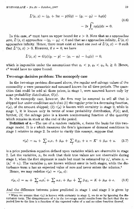
L'(z, x) = (qi + 2-sz p)G(z) - (qi (3.6)
2s J>g(x)dx = 0.
In this case, z* must have an upper bound for s > 0. Note that as z approaches zero, L'(z, x) approaches -(qi qo) < 0 and that as z approaches infinity, L'(z, x) approaches infinity. Hence, there must exist at least one root of L'(z, x) = 0 such that L"(z, x) > 0. However, if s = O, we have
L'(z, x) G(z)(qi 0,
which is impossible under the assumptions that qi < p, qo < qi, bi G; 0. Hence, z* would have no upper bound.
Two-stage decision problem: The monopoly case
In the two-stage problem discussed above, the regular and salvage values of the commodity x were parametric and assumed known for all time periods. The quantities that could be sold at those prices, in stage 1, were assumed known only by some probability distribution, G(x).
In the monopoly case, however, the firm may be assumed to sell all that is shipped but under conditions such that (1) the regular price is a decreasing function, r(µ.), of the amount shipped; (2) r(µ.) is known with certainty in stage 2, while in stage 1, it is known only in terms of some probability distribution, F(e); and, further, (3) the salvage price is a known nonincreasing function of the quantity which remains in stock at the end of the period.
Definition of e.-The use of a random variable, e, forms the basis for this twostage model. It is e which measures the firm's ignorance of demand conditions in stage 1 relative to stage 2. In order to clarify this concept, suppose that
r(µ.) = ao + L a;;~i + f3oµ. + L fliYi + u = K' + fJo.u + u. (3.7) i j
is a price prediction equation defined upon variables which are observable in stage 2. Let the variables, X;, be such that their true values are not observable during stage 1, when the first shipment is made but must be estimated by x/, where x; = (x;' + vi). The variables Yi are known without error in both stages, while the disturbance term u has an expected value of zero and hever enters the solution.8
Hence, we may redefine r(µ.) = r(µ., e):
K + f3oµ. + e. (3.8)
And the dift'erence between prices predicted in stage 1 and stage 2 is given by 8 When we assume that r(µ) is known with certainty in stage 2, we do so by ignoring the dis
turbance term. The disappearance of u in the two-stage model results from the fact. that the expected foss to the firm is a function of the expected value of u and no other function thereof.·
20 BelL: Models of Commodity Transfer
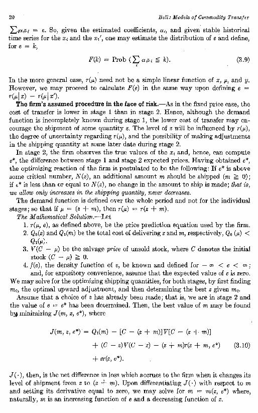
L:iaiVi = e. So, given the estimated coefficients, a;, and given stable historical time series for the Xi and the xl, one may estimate the distribution of e and define, fore = k,
F(k) Prob (l::: a,vi ~ k). (3.9) i
In the more general case, r(µ) need not be a simple linear function of x, µ, and y. However, we may proceed to calculate F(e) in the same way upon defining e =
r(µI x) r(µi x1).
The firm's assumed procedure in the face of risk.-As in the fixed price case, the cost of transfer is lower in stage 1 than in stage 2. Hence, although the demand function is incompletely known during stage 1, the lower cost of transfer may encourage the shipment of some quantity z. The level of z will be influenced by r(µ), the degree of uncertainty regarding r(µ), and the possibility of making adjustments in the shipping quantity at some later date during stage 2.
In stage 2, the firm observes the true values of the X; and, hence, can compute e*, the difference between stage 1 and stage 2 expected prices. Having obtained e*, the optimizing reaction of the firm is postulated to be the following: If e* is above some critical number, N(z), an additional amount m should be shipped (m ;?; 0); if e* is less than or equal to N(z), no change in the amount to ship is made; that is, we allow only increases in the shipping quantity, never decreases.
The demand function is defined over the whole period and not for the individual stages; so that ifµ = (z + m), then r(µ) = r(z + m).
The Mathematical Solution.-Let 1. r(µ, e), as defined above, be the price prediction equation used by the firm. 2. Q0 (z) and Qi(m) be the total cost of delivering z and m, respectively, Q0 (µ) <
Qi(µ). 3. V(C µ) be the salvage price of unsold stock, where C denotes the initial
stock (C - µ) ;?; 0. 4. f(e), the density function of e, be known and defined for - < e < m;CtJ
and, for expository convenience, assume that the expected value of e is zero. We may solve for the optimizing shipping quantities, for both stages, by first finding m 0, the optimal upward adjustment, and then determining the best z given m 0•
Assume that a choice of z has already been made; that is, we are in stage 2 and the value of e e* has been determined. Then, the best value of m may be found bjJ minimizing J(m, z, e*), where
J(m, z, e*) ·= Qi(m) [C (z + m)]V[C - (z + m)]
+ (C - z)V(C - z) - (z + m)r(z + m, e*) (3.10)
+ zr(z, e*).
J( ·),then, is the net difference in loss which accrues to the firm when it changes its level of shipment from z to (z + m). Upon differentiating J( ·) with respect tom and setting its derivative equal to zero, we may solve for m = m(z, e*) where, naturally, mis an increasing function of e and.a decreasing function of z.
21 MONOGRAPH • No. 20 • October, 1967
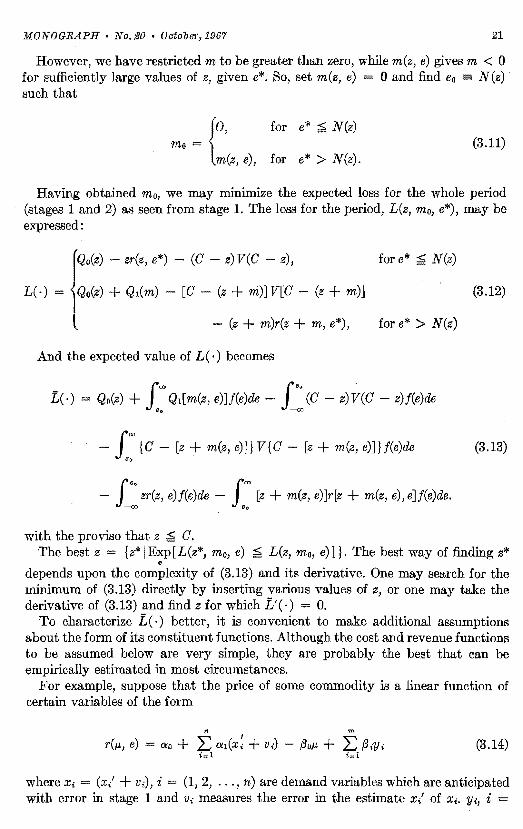
However, we have restricted m to be greater than zero, while m(z, e) gives m < 0 for sufficiently large values of z, given e*. So, set m(z, e) = 0 and find e0 N(z) such that
o, for e* ~ N(z) (3.11){mo = m(z, e), for e* > N(z).
Having obtained m0, we may minimize the expected loss for the whole period (stages 1 and 2) as seen from stage 1. The loss for the period, L(z, mo, e*), may be expressed:
rQo(z) - zr(z, e*) - (C - z) V(C z), fore* ~ N(z)
L( ·) = iQo(z) + Q1(m) - [C (z + ni)] V[C - (z + m)] (3.12)
l - (z + m)r(z + m, e*), fore* > N(z)
And the expected value of L( ·) becomes
L( ·) = Qo(z) + f"' Qi[m(z, e)]f(e)de - f •· (C z) V(C - z)f(e)de e, -oo
- J°" {C - [z + m(z, e)]) V{C - [z + m(z, e)]}f(e)de (3.13).. -f •· zr(z, e)f(e)de - f"' [z + m(z, e)]r[z + m(z, e), e]f(e)de.
---00 ••
with the proviso that z ~ C. The best z = {z*IExp[L(z*, m0, e) ~ L(z, m0, e)] ). The best way of finding z*
c
depends upon the complexity of (3.13) and its derivative. One may search for the minimum of (3.13) directly by inserting various values of z, or one may take the derivative of (3.13) and find z for which L'( ·) = 0.
To characterize L( ·) better, it is convenient to make additional assumptions about the form of its constituent functions. Although the cost and revenue functions to be assumed below are very simple, they are probably the best that can be empirically estimated in most circumstances.
For example, suppose that the price of some commodity is a linear function of certain variables of the form
r(µ, e) = ao + L n
a:i(x: + Vi) (3.14) i=l
where x; = (xl + v;), i (1, 2, ... , n) are demand variables which are anticipated with error in stage 1 and Vi measures the error in the estimate xl of x,. y;, i =
22 Bell: Models ofComm-0dity Tr(J,nsfer
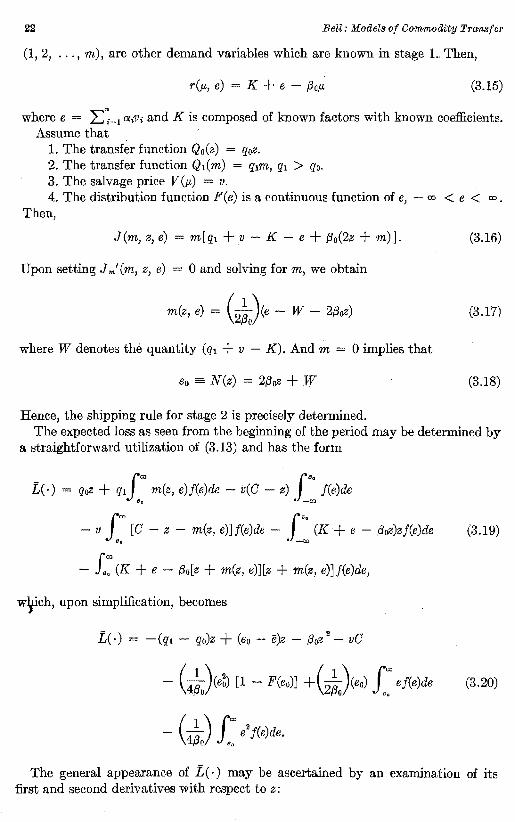
(1, 2, ... , m), are other demand variables which are known in stage L Then,
r(µ, e) = K + e - f3oµ (3.15)
where e = I::_1 rx;V; and K is composed of known factors with known coefficients. Assume that
1. The transfer function Qo(z) = qoZ. 2. The transfer function Qi(m) = qim, q1 > qo. 3. The salvage price V (µ) = v. 4. The distribution function F(e) is a continuous function of e, - oo < e < oo.
Then,
J(m, z, e) m[q1 + v - K - e + f3o(2z + m)]. (3.16)
Upon setting Jm 1(m, z, e) = 0 and solving form, we obtain
m(z, e) = C~)(e - W - 2f3oZ) (3.17)
where W denotes the quantity (q1 + v - K). And m = 0 implies that
eo = N(z) = 2{3oZ + W (3.18)
Hence, the shipping rule for stage 2 is precisely determined. The expected loss as seen from the beginning of the period may be determined by
a straightforward utilization of (3.13) and has the form
LC·) qoZ + qifco m(z, e)f(e)de .. - v(C z) J•· f(e)de --OJ
v f"" [C.. z - m(z, e)]f(e)de J.. (K + e --OJ
- (3oZ)zf(e)de (3.19)
- J.~ (K + e - f3o[z + m(z, e)]lz + m(z, e)] f(e)de,
wjich, upon simplification, becomes
L(-) = -(qi - qo)z + (eo - e)z - f3oz 2 vC
- C~J(e~) [l - F(eo)] +(2~)(eo) f~ ej(e)de (3.20)
2-C~) f~ e f(e)de.
The general appearance of L( ·) may be ascertained by an examination of its :first and second derivatives with respect to z:

23 MONOGR.t{PH • No. 20 • October, 1967
J"' ef(e)de, (3.21)
and
L"(·) = e~F(eo).
L'(.)
The minimum of L( ·) occurs at a value of z for which L'( ·) = 0, and L"( ·) > 0. Now, if we make the logically necessary assumption that F[e0(z)] ,..,., 0 when z = 0, it follows that as z approaches 0, L'( ·) approaches -(qi"- q0) < 0 and that as z
. approaches infinity, L'( ·) aproaches infinity. Hence, L'( ·) must possess at least one root. Moreover, since L"( ·) ~ O, L1
( ·) is a monotonically nondecreasing function of z and, therefore, may possess at most one real root. This simple root defines z*. So, in searching for the minimum of L( · ), it is sufficient to find any z0
such that
L(z0 + "A, m0, e) > L(zO, mo, e) < L(z0 "A, mo, e)
for arbitrarily small "A. 9
For computational convenience, if w is any normally distributed variable with a zero mean and a known variance u2
, it possesses the density function
- 1 _,,,' 12/f(w) - ---e uy2'11"
for oo < w < m and has the convenient property that
and
(These equivalences are proven in Hadley and Whitin, 1963, p. 144.) Upon utilizing (3.22) in further simplifying the expression for the loss function
given by (3.20), we obtain
L(·) = -(qi - qo)z + eoZ - (3oZ2
- vC
(3.22)
(3.23)
Since both F(eo/u) and f(eo/u) are easily obtained from published tables, (3.23) offers itself well for numerical computations.
9 For a numerical example of the two-stage model, see page 36, "An Example of the Dynamic Two-Stage Model."
24 Bell: Models of Commodity Transfer
Characteristics of the two-stage model
Equation (3.20) reduces further to
L(·) qoZ + {3oZ2 - v(C - z) - Kz + M(z)
where
M(z) = -C~)e~[l - F(ea)] + (2~)eo f~ef(e)de C~) f~e2f(e)de . (3.24)
Note that M(z) contains all of the random elements of L( ·)and that the remainder of L( ·) is nothing more than the net loss function for the riskless situation. Moreover, M(z) may be shown to be the advantage, as a function of z, of the existence of stage 2.
Proof: Assume that there is no stage 1; that is, the firm always waits until it has observed e* before making its single shipping decision for the period. Then, the firm's actual net loss for any period is given by
H(m) = qim - v(C - m) - (K + e* - f3om)m (3.25)
and the optimal, loss-minimizing policy is to ship m*, such that
H'(m*) q1 + v - K e* + 2f3om* = 0
and
m* = (_!_)(e* - W) (3.26)2f3o
where W (q1 + v - K).
If m* is constrained to be nonnegative, then m* 0 fore ~ Wand the expected value of H(m*) is.
H(m*) = (2~)(q1 + v). f.ce W)j(e)de vC
00 00
2
, - C~) J. (K + e)(e - W)f(e)de + C~) J. (e - W) f(e)d<
(3.27)
-C~)w2[1 F(W)] + (2~) W _£:f(e)de vC
C~) f.00
e2f(e)de.
Now, note that eo = = M(O) ! Q.E.D.2f3oz + W, so that W= eo(O), and 11(m)
25 MONOGRAPH • No. 20 • October,1967
In the riskless case, the optimal shipping quantity, z0*, is that which minimizes
Lc(z) qoZ - v(C - z) - (K - /3oZ)z (3.28)
and zo* must satisfy
(3.29)
In the case of risk, however, the optimal shipping quantity, z,*, say, is that which satisfies the condition that
where
00 1
M (z) = f ef(e)de - eo[l F(eo)J • (3.30)., Now, -Lc'(z) is the marginal net revenue function for the riskless case, and,
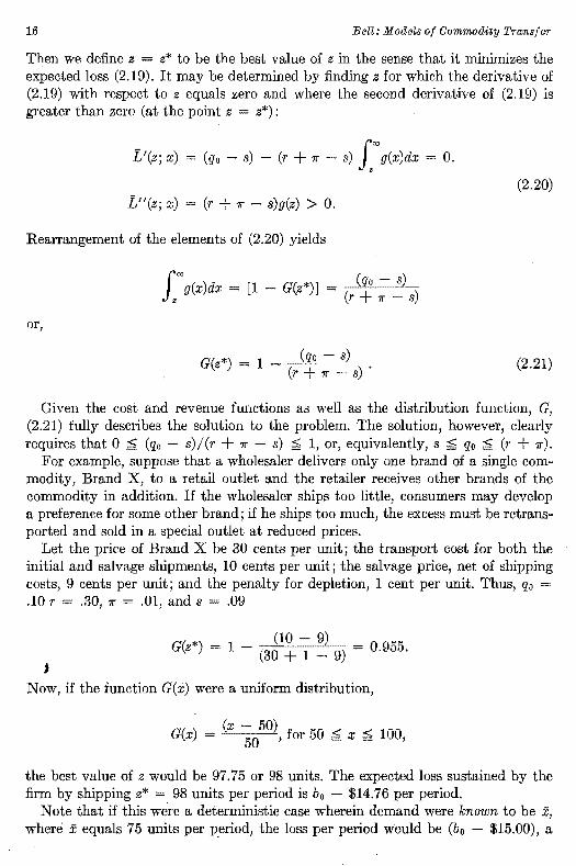
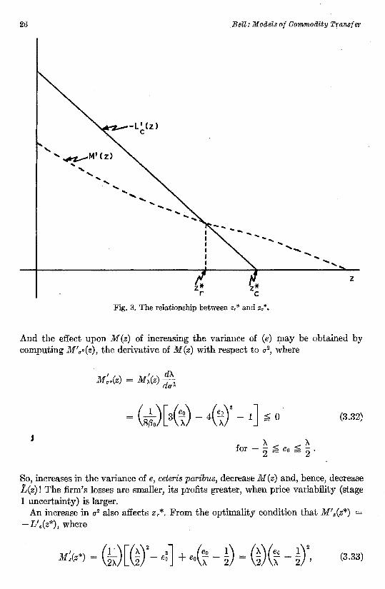
given the rather simple functions which we have been employing, - Le' (z) is a line of slope -(2/30), with K (q0 + v) as an intercept. The general appearance of M'(z) may be deduced from the fact that M"(z) = -2/30 (1 - F(e0)) and that lim M'(z) = O; M'(z) must, in general, decrease at a decreasing rate approaching•-oo zero asymptotically. Moreover, M"(z) ~ -2/30, where the equality holds only for F(e 0) = 0. Hence, if the intercept of M'(z) is below that of -Lc'(z), then, M'(z) =
-L/(z) for some positive value of z, and, of course, this intersection defines z,*. See figure 3.
The effect of variations in q1.-Assume that F(eo) = O, for z 0, so that M 1(O) = -e0(0) = K (ql + v). Then the intercept of M 1(z) will be less than that of -L/(z) by the amount (ql qo). Hence, if ql;;;;; q0, then z,* = O; and, as (ql - qo) grows larger, the intercept of M1 (z) falls and z,* increases. And since
-[1 - F(eo)] ~ 0,
we know that increases in q1 decrease the slope of M'(z) for every z for which F(e 0) < 1 and do so to an extent which is inversely related to the size of z.
The effect of variations in the variance of e.-Because it is difficult to indicate precisely the effect upon M(z) of variations in the variance of e, we shall confine ourselves to investigating the particular casef(e) = 1/).., for -X/2 ~ e ~ "J../2.
If f(e) l/X, then
M() = + eo._ (3.31)(i)(eo3
z 4f3o 3").. 4
2fi Bell: Models of Commodity Transfer
..... '~M1 (z) ... ..... .... ........ .... .... .... .....
.... ........
- ...... ..... .... _ ..... ... ........
z
Fig. 3. The relationship between e,* and z.*.
And the effect upon M(z) of increasing the variance of (e) may be obtained by computing M'~·(z), the derivative of M(z) with respect to (f
2, where
(3.32)
J A< <~for 2 = eo = 2.
So, increases in the variance of e, ceteris paribus, decrease M(z) and, hence, decrease L(z) I The firm's losses are smaller, its profits greater, when price variability (stage 1 uncertainty) is larger.
An increase in a2 also affects Zr*· From the optimality condition that M'.(z*) = - L'c(z*), where
(3.33)
27 MONOGRAPH • No. 20 • October, 1967
we obtain
(3.34)zt = (2~) [ K - (qo + v) - ~(~ - ~YJ and
3 eo I < A.< < A. ( 2X/3o)[(i )
2 - 4J = O, for - 2 = 60 = 2 · (3.35)
Hence, an increase in o-2 reduces the optimal z,* and, consequently, increases the frequency and size of stage 2 adjustments.
The desirability of price variability.-Since M;(z) is a non-negative function which approaches zero (perhaps) asymptotically10 as z approaches infinity and since lim M(z) is clearly zero, we know that M(z) is a monotonically increasing, non.....,, positive function of z and that when M.'(z) 0, M(z) ,....., 0. Hence, if M/(z0* ,..., -Lc'(zc*) so that z,* ,....., zc*, then we know that M(z.*) = 0. And if M.'(0) = -Lc'(O), that is, if the point of intersection in figure 3.1 is for z = O, then M(z,*) H(m). See equation (3.27).
Now, recall that M(z) was said to be the advantage (as a function of z) of the existence of stage 2. By this we meant that for any z which is selected in stage 1, M(z) measures the additional reduction of net loss which may accrue to the firm if, in stage 2, it is possible to make an upward adjustment of size m* = [I/(2J3o)] (e - e0).
-0../2.) 0 0./2)
1 (- --)
860
M I u2(z)
I I
I I I I I I I / I /I /I / I /I / I "/l ,
----- ---............ II """ '\"' ....... _ ....._, I ..-*"'-..... ,....,,. ,,, M1,,,'' (z)
,,,.,,. a2
,,' ,,"
,"' "' _.... ,,,,,,,"'
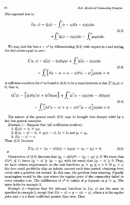
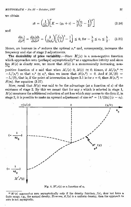
Fig. 4. M'.•(z) as a function of eo.
io 1111(z) approaches zero asymptotically only if the density function, f(e), does not have a finite range, e.g., the normal density. However, if f(e) is a uniform density, then the approach to zero is not asymptotic.
28 Bell: Models of Commodity Transfer
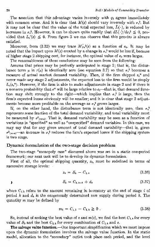
The assertion that this advantage varies inversely with qi agrees immediately with common sense. And it is clear that M(z) should vary inversely with a-.2. But it may not be clear that the value of the total expected loss, L( · ), is reduced by increases in a-.2. However, it can be shown quite readily that dL(·)/du 0
2 ~ 0, provided that Lc'(z) ~ 0. From figure 3 we can observe that this proviso is always satisfied.
Moreover, from (3.32) we may trace M~.2(z) as a function of e0• It may be noted that the impact upon M(z) created by a change in ul- would be less if, because of higher stage 2 shipping cost, for instance, the optimal value of e0 were larger.
The reasonableness of these conclusions may be seen from the following: Assume that prices may be perfectly anticipated in stage 2; that is, the distur
bance term µ in r(µ) is identically zero (see equation 3. 7) so that a •2 becomes a measure of actual market demand variability. Then, if the firm shipped zc* and never made any stage 2 adjustments, the expected loss to the firm would be simply Lhc*). However, if the firm is able to make adjustments in stage 2 and if there is a nonzero probability that e* will be large relative to e0-that is, that demand function may shift strongly to the right-which implies that u •2 is large, then the firm's expected losses obviously will be smaller; and it is clear that stage 2 adjustments become more profitable on the average as u •2 grows larger.
If, on the other hand, the disturbance term is not identically zero, then a •2 .
represents some fraction of the total demand variability, and total variability must be measured by u2 ce+uJ· That is, demand variability may be seen as a function of variations in "specified" as well as "unspecified" demand variables. In this case, we may say that for any given amount of total demand variability-that is, given a 2ce+u)-an increase in u.2 reduces the firm's expected losses if the shipping system is two stage.
Dynamic formulation of the two-stage decision problem The two-stage "monopoly case" discussed above was set in a static one-period
framework; our next task will be to develop its dynamic formulation. First of all, the optimal shipping quantity, zk, must be redefined in terms of
successive storage levels:
(3.36)
, (3.37)
where Ci, k refers to the amount remaining in inventory at the end of stage i of period k and dk is the exogenously determined new supply during period le. The quantity m may be defined by
(3.38)
So, instead of seeking the best value of z and m(z), we find the best Cl. 1r for every value of Sk and the best Cz k for every combination of Cu and e.
The salvage value function.-One important simplification which we must impose upon the dynamic formulation involves the salvage value function. In the static model, allocation to the "secondary" outlet took place each period, and the level
29 MONOGRAPH • No. 20 • October, 1967
of stock was always reduced to zero. For the dynamic case, however, such a procedure is suboptimal since stock carried over from one period may be used in the priority outlet during the next period. The consequence is that there are now three decisions to be made during any period: a choice of z, m(z) and s[z, m(z)], say, where s( ·) is the amount sent to the secondary outlet during the period. The result is that the "static" two-stage problem leads to a three-stage dynamic problem.
One of the simplest ways of maintaining the two-stage characteristics of the dynamic process is to place all of the salvage operation at the end of the season. The result would be that each period is two stage and the last period would have a loss function of the same form as that observed in the static models.
However, relegating all salvage to the last period-period t- forces the model to carry, on the average, a higher level of inventory than the real process if in the actual process salvage is distributed throughout the season. This distortion of the average level of inventories may be sufficient to destroy the usefulness of the model if "holding cost" is included as a significant factor.
Although the cost of holding produce in storage is an important cost element in many shipping processes, this is our first occasion to mention holding cost since our discussion of deterministic systems. The omission of this factor in the static versioas of the multistage decision problems was based upon the implicit assumption thnt such. cost was insignificant because of the meagerness of the unit cost itself or because of the relative briefness of the shipping period, or both.
In the dynamic case, however, we face the possibility of having to carry large levels of inventory over relatively long spans of time, and it is proper to reconsider the cost-of-holding factor.
If it is desired to recognize the cost of holding, it is probably best to completely eliminate from the system that part of the crop which is destined for the salvage outlet. One method of doing this would be to predetermine, perhaps by use of a deterministic model, the quantity which will be delivered to salvage and the intraseasonal distribution thereof and subtract those quantities from the dk. In this way we may prevent the appearance of any exaggerated storage levels in the model.
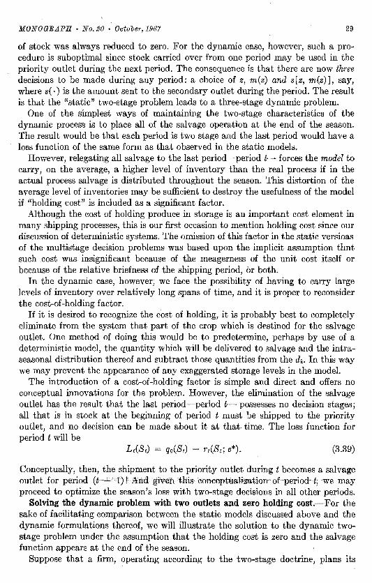
The introduction of a cost-of-holding factor is simple and direct and offers no conceptual innovations for the problem. However, the elimination of the salvage outlet has the result that the last period-period t- possesses no decision stages; all that is in stock at the beginning of period t must be shipped to the priority outlet, and no decision can be made about it at that time. The loss function for period t will be
(3.39)
Conceptually, then, the shipment to the priority outlet during t becomes a salvage outlet for period (t·.;.;;. 1)!' And given this conceptualization· of·period- t; ·we may proceed to optimize the season's loss with two-stage decisions in all other periods.
Solving the dynamic problem with two outlets and zero holding cost.-For the sake of facilitating comparison between the static models discussed above and the dynamic formulations thereof, we will illustrate the solution to the dynamic twostage problem under the assumption that the holding cost is zero and the salvage function appears at the end of the season.
Suppose that a firm, operating according to the two-stage doctrine, plans its
30 Bell: Models of Commodity Transfer
shipping pattern over a horizon of t periods. For each period t - j, there exists a loss function-Lt-i( ·)-such that for at least one period-say, the t-pth periodLt-i( ·) ~ Lt-p( · ). That is, assume that the system does not possess stationarity. Then, the firm must find a sequence of functions, C2, t-i = C0t-i and Ci, t-i = wi, t-i(St-i); j = 0, 1, 2, ... , t. This set of functions will define an optimal policy if it minimizes
1/;o, t = :ELo Exp Lt-iC1, t-i, C2, t-i; St-i, e) - V(C2, t) . (3.40) e
The expected loss for each period, Lt-i( · ), has the same form as the loss in the one-period model; but, with the difference noted above, the salvage-value function operates only upon the last period.
Hence, for any period other than .the very last, Lt-l ·) is given by
Qo(St-i - C1, t) + f'° Qi(C1, t-i - C~-i)f(e)de.. (3.41)
- f'° (St-i - C~-i)rt-iSt-i - de-i, e)f(e)de • .. And the loss sustained during period t is of the same form as (3.41) but with the addition of the salvage-value function
V(Ct) = J•• C1,1V(C1,1)f(e)de + f'° C~V(C~)f(e)de. (3.41a) -co ••
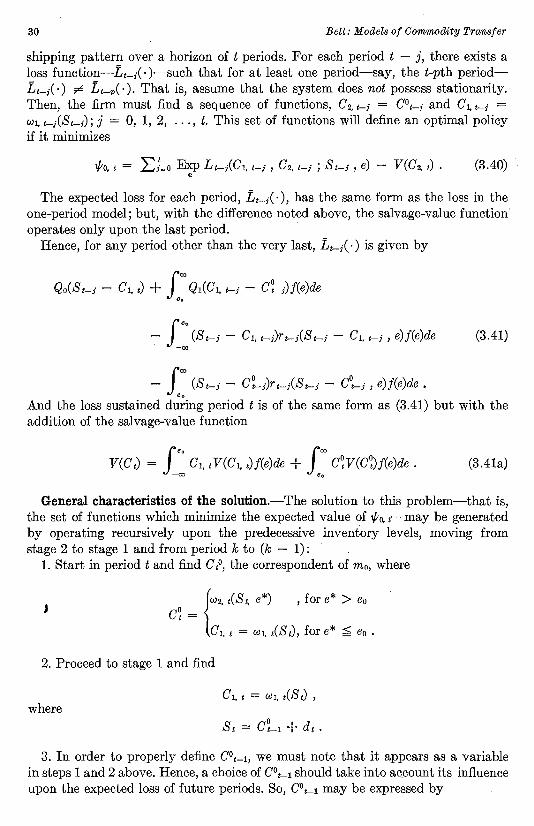
General characteristics of the solution.-The solution to this problem-that is, the set of functions which minimize the expected value of 1/;o, t-may be generated by operating recursively upon the predecessive inventory levels, moving from stage 2 to stage 1 and from period k to (k - 1):
1. Start in period t and find Ct0, the correspondent of mo, where
{w2, 1(S t, e*) , fore* > e0 J 0
Ct= C1, t = w1, 1(S1), fore* ~ eo .
2. Proceed to stage 1 and find
where
3. In order to properly define C01_1, we must note that it appears as a variable
in steps 1 and 2 above. Hence, a choice of C0t-I should take into account its influence
upon the expected loss of future periods. So, C01_ 1 may be expressed by
31 MONOGJJd.PH • No. 20 • October, 1967
{w2, 1-1(w1, t(S1); S1-1, e*), fore*> e0 0
Ct-1 = w1. t-i(S i-1) , fore* ~ eo •
4. Continue this procedure until period (O) is reached. Having reached j 0, one will have found for every time period and each stage a function defined upon the stock level of that period which provides the optimal level of carryover. Hence, if we are in period k, we may observe the true value of Sk and obtain a numerical value for the optimal Ci. k·
The exact solution of a special case In following the procedure outlined above, one may seek the various minima by
tracing the total loss function directly, or one may take the derivative of 1/li., with respect to each level of carryover. Utilization of the total loss function provides the most practicable route to solution; however, in order to give a general characterization of the solution we are forced to use the derivatives. ·
The characterization of the problem which we present below is rather simple and direct, but this simplicity comes at great cost: we are forced to consider w;, k(Sk) for a restricted range of Sk, and the transfer function for stage I must be of the simple linear form which has been used heretofore; that is, Q0(z) must be q0z.
The restriction of the range of Sk is to Bk-sufficiently-large such that neither stage I nor stage 2 shipments will ever be effectively constrained by the storage level. And Qo(µ) must be kept simple in order to make it possible for the optimal rule of any period to be expressed as a function of eo, 1 alone. The impact and importance of these restrictions will be made clearer as we proceed.
In this example, the only function which differs from those used earlier is the salvage-value function.
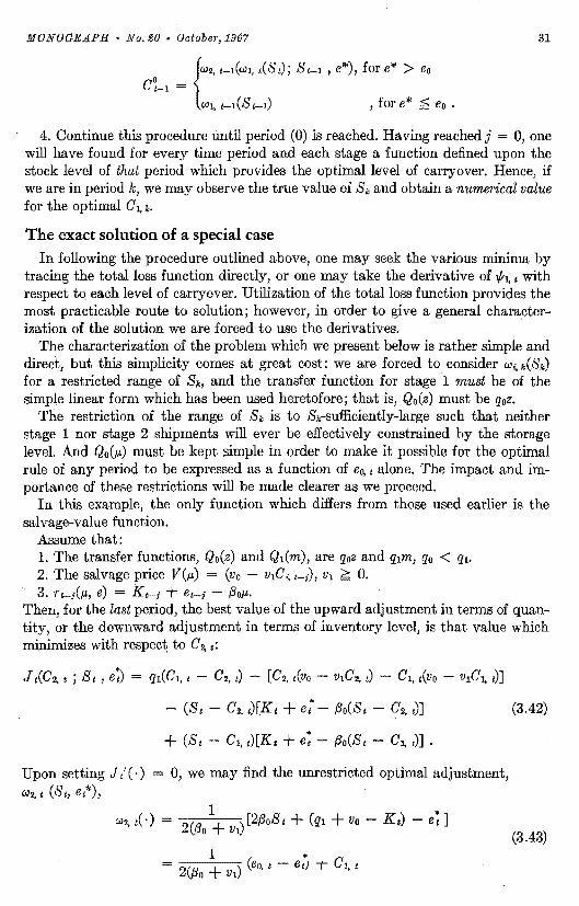
Assume that: 1. The transfer functions, Qo(z) and Q1(m), are qoz and qim, q0 < q1• 2. The salvage price V(µ) (vo - v1C~t-i), v1 ~ 0. 3. ri-i(µ, e) = Kt-f + ei-f - f3oµ.
Then, for the last period, the best value of the upward adjustment in terms of quantity, or the downward adjustment in terms of inventory level, is that value which minimizes with respec~ to C2. t:
- (Si (3.42)
Upon setting J /( ·) O, we may find the unrestricted optimal adjustment, w2. t (St, e1*),
(3.43)
32 Bell: Models of Commodity Transfer
where (3.44)
So, the actual adjustment will be
Now, we proceed to stage 1 of period t and derive C*i. t = w1, 1(St). The optimal C1• 1 is the level of carryover which minimizes L1(C1, 1; S,), where
- (St - C1, t)[K1 - /3o(St - C1, t)] + 2(/0~ ) ("' ef(e)de (3.45) o V1 Jeo, t
L1( ·) possesses a global minimum where
L;( ·) = (q1 - qo) - e~. 1F(eo, 1) - 1: ef(e)de = 0 . (3.46) eo, t
Equation (3.46) is a function of e*0• t alone. Hence, given an initial storage level, 81, it is sufficient to find the value of C1, 1, which satisfies (3.44); call that value C*1, 1•
Of course, C*1, t must be greater than zero; it must be large enough to accommodate the largest probable stage 2 adjustment. These conditions imply that the value of S, must be above some lower bound if equations (3.45) and (3.46) are to be meaningful. The lower bound of the set of admissable S 1, to be called "St'Il ," will be determined below, see page 35. But in the meantime, we will simply remember that our discussion depends ultimately upon the specification of S/f!. So, given e*o. 1 from (3.46), we know that C*1, 1, the optimal stage 1 adjustment, is a function of S 1 alone. From (3.44) we obtain
J c~. t 2(fto ~ v1) ~oSt + (q1 +Vo - Kt) e~.} • (3.47)
Given the C*t, 1 and e*o, 1, the value of the expected optimal loss for period t, say Liw(Si), may be defined for any St ~ S/Il. The derivative of L1w(S1), with respect to S 1 is one of the most significant elements of the multiperiodic process. It is this derivative which relates each period to its successor; it takes on the role of the salvage value function for earlier periods.
- I 2 * * L1w(S 1) = (1 - B 1) [eo, t - (q1 - qo)] - (vo - 2v1C1, 1) (3.48) where
B = dC~. t _ /30 (3.49)t - dS t - /30 + V1
33 MONOGRAPH • No. 20.• October, 1967
Period (t - 1). - We may define Ji-n( · ), where J t-n( · ), for any n > O, is identical in form to J,(·), except that V(µ) is replaced by Liw(S1); and since 8 1 = (C2, 1-1 + di), the derivative of Liw(St) with respect to C2, i-1 is L/w(Si) as defined in (3.48). Hence,
dJ~-1(.) - • - [K1-1 - qr + e1-1 - 2/30(81-1 - C2. 1-1)]
dC2, t-1
(3.50) +(1 - B 1)
2[e~. i - (q1 - qo)] Vo + 2v1C;, t = 0 .
And given (3.49), we know that C*1, tis a linear function of 81, for 8 1 > S(B, so that a scalar, A 1*, can be defined such that
(3.51)
• /30 (= At+ r:i + C2, t-1 +di)./"O V1
By employing (3.51) with (3.50), we obtain (for e*i-1 $;; eo, 1-1)
/30 + V1 { s KC2, t-1 = 2/3o({Jo + 2vi) 2/3o 1-1 - t-1
(3.52)
V12 • • }- (/3o + v ) 2 [eo, t - (q1 - qo)] + Vo - 2v1(A t + B t d2) . 1
In order to find the optimal rule for stage 1, we construct the function Li-1( ·) which is identical in form to (3.41) with the addition of L1UJ(C1, t-1). The derivative L' 1_ 1 ( • ), can be shown to have the same form as L/( ·):
f<D
- ' * *L 1-1( ·) = (q1 - qo) - ea, 1-1F(eo, 1-1) - * ef(e)de = 0 . (3.53) tlo, e-1
Hence, if F(e) is the same for periods t and t 1, then e*o, 1-1 = e*o. 1; and C*1 1-1
is the level of carryover which satisfied (3.52) when e* t-1 = e*0, 1-i and, consequently C2, t-I = Ci, t-1=
(3.55)
34 Bell: Models of Commod-ity Transfer
Finally,
(3.56) + (1
where
B _ dC~. 1-1 (3.57)t-i - dSi-1
and
c~. 1
,. f3o [( " f3o + V1 ) J = At+ f3o +Vi At-1 + f3o + 2v
1 81-1 + dt (3.58)
* .. f3o At+ f3 + (A1-1 + dt) + (3 + 2 81-1.
O V1 o V1
The remaining periods.-At this point it is possible to observe the pattern which the various functions are assuming. The only factor which produces any distinction between the loss functions of different periods is to be found in the expression for the derivative of the optimal loss, L1-iw(S1-n). The behavior of L11_,,w(St-n) is indicated in (3.56). Simple induction indicates that
n
[e; - (qi - qo)] :E }=O
where {3 0 + (n + l)v1 is the denominator of Bt-n [see (3.57) and (3.51)] and
c~. t = (3.60), [see equation (3.58)].
Careful examination of the process of deriving L1-1( ·) indicates that
L1-n( ·) = (q1 - qo) - eo, t-n F(eo, 1-n) - f~ ef(e)de eo, C-11
holds for all n, so that e*o, 1 = e*o, t-n provided that the distribution function, F(e), is the same for all periods.
Given that e*o, 1-n = e0*, it is possible to generate optimal stage 1 transfer rules
0
35 MONOGRAPH • No. 20 • October, 1967
over the entire horizon. An expression for C*i. 1_,. can be found for all n, t > n ~ 0 by use of (3.54):
Ki-n) - e;J (3.61)
where
Bt-.. (3.62)f3o + (n + l)v1
and
(3.63)
n-1 2 * ~ V1+ [eo - (q1 - qo)] L.J [{3 + ( · + l) ]2 ·
i=O 0 J 1!1
Or, if we rewrite (3.61) in order to isolate certain elements
n-1
c;, t-n = Bi-nSt--n + H(n) - Bt-n L:-~--,- (A~-i + dt+H). (3.64) j-0
Equation (3.64) makes clear the fact that the solution of the multiperiodic process may be reduced to the problem of determining the values of A *i-;, J = 0, 1, 2, ... , t. These values may be determined quite simply through a recursive iterative pro
. cedure. Note that the numerical solution for C*i. t-n, given some initial storage level, say S0
1_,,,., requires nothing more than the values of the basic parameters and the values of the A*t-i> J = 1, 2, ... , n - L Given these values, C*i. t-n(S0t-n) is immediate. Moreover, A *t-i may be quickly determined as the value of the intercept (on the "y" axis) of the line with slope Bt-i through C*i. t-i(S0H) (see figure 5, page 39). Finally, the stage 2 adjustment can easily be expressed as
(3.65)
where
V t--n( ·) - K t-n) . (3.66)
The determination of SEF! i-,,.-Having completed the derivation of rules which are optimal for the system which maintains St-n ~ srn i-n, n = 0, 1, 2, ... , t, it is easy to determine Sffi t-n·
The most obvious requirement for S© t-n is that it be sufficiently large to prevent C*z t-n from becoming negative. Let em denote the largest probable value of e for
36 Bell: Models of Commodity Transfer
which F(e) > 0. Then, the first requirement for St--n ;:;;;; S 63 t-n follows from (3.65):
0 ;;;;;; (2~)B1-n(e~ em) + ~. 1-n, n = 0, 1, 2, ... , t
or
0 ;;;;;; (2/Jo1)B 1-n(eo.. - e,,,) + A
. t-n + B t-nS t-n • (3.67)
The more complex requirement on S 63 "--"is a consequence of the dynamic process. Given the transfer rules and given the exogenous storage input series, di-ii we must require that St--n be large enough to insure that there will be no supply deficiencies in future periods. This criterion may be handled by an elaboration of (3.60).
Observe that (3.60) offers a relationship between St-n and C*i, t· The lowest permissible C*i. H (for any j) is [ 1/(2.Bo) JBt-i(en eo*); hence, S!JJ t-n must satisfy
1 ) • ~ .Bo( B 1(em - eo) ;;;;;; ~ r.i + . (A t-i + d1+1-1)2{3o) 1-0 {JO JV1
(3.68)
.Bo Ell
+.Bo+ (n + I)v1 St-'":·
It is possible for St-n to satisfy (3.67) and (3.68) and still fail to be large enough to insure C*2, t--k 6 0, for some k, 0 < k < n. To handle this case, it is sufficient to find the analog of (3.60) for C*i, t-k, k 6 0
• ~ .Bo + kv1 • )Ci, t--k = L... f3 + . (A t-1 + d1+1-f
i-k o JV1
(3.69) .Bo + lcvi EfJ
+.Bo +(n + l)vi St-n, k = 0, 1, 2, · · · , n.
Now note that (3.69) holds for all k, n 6 le 6 0. Further, if we add the stage 2 condition to (3.69), we will have specified sufficient conditions for St-i ;:;;;; Sffi t-i: ,
0;;;;;; (2~0))B1-k(e~ em)+ :t .Bo+ jvi (A~-i + di-+1-1)
(3.70) .Bo + kvi sfF!
+ f3o + (n + l)v1 t--n
for n ;:;;;; k ;:;;;; 0. Equation (3.70) says that sm t-n is the storage level just large enough to com
pensate for any future deficiency in future supply. If the di+i-;, j ;;;;;; n are rather large, then it is likely that SfJJ t-n will be defined by its "own period" conditions (3.67). But if the dt+l-i are decreased (ceteris paribus), SEil t--n will tend to become effectively constrained by some future period condition.
37 MONOGRAPH • No. 20 • October, 196'7
An interesting property of (3.70) is the declining sensitivity of the condition, C*2, t-i ~ 0, to changes in St-n as (n j) increases. Hence, if the system is to avoid greatly exaggerated values of sei t-n, for large n, the dr.+l-i should be such that sei t-n will tend to be defined by the own-period conditions.
An example of the dynamic two-stage model Assume that
1. Stage I and stage 2 transfer costs qo and q1 are 2 and 4, respectively.
2. The salvage value function is (2 .IC;, 1-;)Ci, t-i·
3. The slope of the demand function is 0.2, with intercepts, Kt-i, at 40, 30, and 50 in periods t, t - 1, and t 2, respectively.
4. At the beginning of each period, 100 additional units come into storage; i.e., dt = dt--1 dt--2 100.
5. And the random variable, e, has a normal distribution with an expected value of zero and a variance equal to two.
Period t.-From equation (3.46) we know that the optimal value of e0 must satisfy
And by trial and error, we find that e*0 = 1.84. Now we know from (3.44) that
e~ = 2{3(S t C~. 1) or
1.84 = .4(S t a;, 1) - .2a;, t + (4 + 2 - 40)
and if Si 200 and 200 ~ sei1, then
c;. 1(200) = 73.6 .
From (3.51) or (3.60) one can find G*i, t for every S 1 ~ seit since all other G*1. 1
lie on the line with slope fJo/(fJo + v1) = 2/3 which passes through 73.6 (see figure 5 below):
• '· 6l2G1, t = -59.8 + 381, for S1eS1.
Period t - 1.-Since e*o,t = e*o,t-n, for all n, we know from (3.54) or (3.61) that
C~. t--1 = 2.5 (~) [.4S t-I + (4 + 64 - 30) - 1.84] .
Hence, if we assume that S1_1 = 200 and that 200 ~ sei t--1, then we may solve directly for G*i, 1-1, obtaining
c~. 1-1(200) = 99.o .
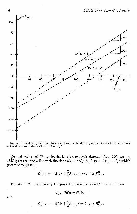
38 Bell: Models of Commodity Transfer
100
BO
60
40
20
0
-20
-40
-60
-80
-100
20 40
,, ....
,, ....,,
....,, ....,,
,, ....
100
....
"" ....
,,
/ 120/ 140 160 180,,,,
.... .... st .-J
,, ,, ....
,, / ....
er. , t-·J
/
,, / ,,,,,,
Fig. 5. Optimal carry-over as a function of St-1. (The dotted portion of each function is nonoptimal and associated withs,_; ;:;;; S®t-;.)
To find values of C*1, 1-1 for initial storage levels different from 200, we use (3.-h2); that is, find a line with the slope ({30 + nv1)/[f30 + (n + l)vi] = 3/4 which passes through 99.0
c~. 1-1 51.0 + ~S1-1, for S1-1 ~ S~i.
Period t - 2.-By following the procedure used for period t 2, we obtain
c~. 1-2(200) = 63.04 and
~ 4 9 Ci. 1-2 = -97.0 + 581-2, for S1-2 ~ Si-2.
39 MONOGRAPH • No. 20 • October, 1967
S(JJ t-n·-The set of admissible S1_,,, has not yet been delineated for the above example.
Since e is a normal variate with a zero mean and a variance equal to two, the maximal value of e for whichf(e) > 0 may be assumed to be less than 10, say, 9.84.
Then, by employing (3.69), we find that SEl'! 1 = 109.5; SEl'! 1-1 = 88.2; and Sffi 1-2 =
142.25. (These values of SEl'! H correspond to the boundary derived when j n in (3.69) for each n. This is a result, however, of the fact that the d 1_,. is fairly large.)
· The definition of e in a dynamic framework
We initially defined e for the static model. In that case, we were able to confine ourselves to price anticipations of only one period. Recall that we said: e = r(µlx) r(µ Ix'), where x is known in stage 2 and only its predicted value x' is known in stage 1. In the dynamic problem, however, e must be defined for all future periods as well, in spite of the fact that x/ may not be known until period t.
The escape from this dilemma is simple, uncontrived, and illustrative of the information seeking aspects of the model:
If we are in period t j, and x/ is not known, then it is sufficient to utilize any unbiased estimate of xi' and therewith solve for the optimal policy of the (t-j)th period. Then, if in period (t - j + 1) we possess a better estimator .of x/, we should solve for the (t j + l)th policy using this better estimator, and so on.
In general, if we are willing to recompute the entire dynamic solution during each shipping period, starting from period t, we are able to interject into the process any available quantifiable demand and supply information about any present or future period.
The only asymmetry in this procedure is that f(e) should never be defined in terIDB of, say, x", the predictor of x'. To do so would force the distribution of e of future periods to have a larger variance than otherwise, overstate the degree of ignorance possessed in stage 1 relative to stage 2 of future periods, and thereby overstate the probability that in future periods there will be a strictly positive µpward adjustment in stage 2. This, in turn, would understate the expected economic loss over the remainder of the season. 11
Unless the investigator has some definite reason for experimenting with distributions one which are defined upon successive approximations of x', it is probably better to definef(e1) from e1 = r1(µlx) r1(µlx') even before x/ is directly observable.
A three-stage decision problem
Consider an extension of the two-stage system of the following sort: Let the shipping stages and shipping decisions be the same as in the two-stage problem, except that once the quantity (z + m), m $:;; 0 and z > O, has reached its final destination, it is possible for the shippers to withhold from sale any percentage of
11 In our characterization of the two-stage model [see equation (3.32)], we found that d [L(.)] / da2 ~ 0.

40 Bell: Models of Commodity Transfer
the shipped quantity, in view of additional information with respect to demand, if to do so appears to minimize the loss of the period's operation.
Such a system may be realized by assuming the 'existence of a third distinct, nonoverlapping stage in which a quantity X, /.. 2 0, may be shipped, depending upon the observed value of some random variable u where u has a definition similar to that of e.
Let the unit cost of transfer in stage 3 be % q2 < 0, Iq2 / > q1 > qo; and assume that the variable u has a known distribution function G(u). Otherwise, let us retain the assumptions with respect to revenue and cost functions which were employed in the monoperiodic two-stage problem.
Optimization in the third stage.-Suppose that we start in stage 3 subsequent to the selection ofµ = (z + m) and the observation of both e* and u*. Then if minimization of the period's loss requires the withholding of some amount, -/.., from sale, /..will be determined as the value which minimizes H(µ,X,u) where
H(µ, X, u) = q2X - {v[C - (µ + X)] - v(C ~ µ)}
(3.71)
- {[K + e* + u - f3o(µ. + X)](µ + /..) - (K + e* + u - f3oµ)µ} •
To find the best X, we take the derivative of H with respect to /.. and set it equal to zero, obtaining
X(µ., e', u) = C~)(u + e' - U - 2(30µ) (3.72)
where U (q2 + v - K) and /..(µ, e*, u) represents an unrestricted (in sign) adjustment in the shipping quantity. However, if /.. is restricted to be nonpositive, then (3.72) is relevant only for u 2 uo, where
Uo = 2(3o/l + U - e* (3.73)
and the actual adjustment in the third stage is
, 0 , for U ~ Uo
Xo = (3.74){ /..(µ, e*, u), for u < uo.
Optimization in the second stage. To find mo, the optimal adjustment in stage 2, we must find the minimum of some function, J(µ, X, e*, u), with respect to m. This function will be conceptually the same as H, except that we must now consider four possibilities: m 0, /.. O; m O, /.. < O; m > 0, /.. = O; m > 0, /.. < O, and
Prob(XIX < 0) = fu" g(u)du . __,,,

41 MONOGRAPH • No. 20 • October, 196'!
It is important to note that if m = 0, uo is a function of z and not of (z + m), m ~ 0. Hence, in expressing the expected loss for the period as it appears in stage 2, the definition of u0 must vary, corresponding to different assumptions with respect to m. Let uo(µ) and u 0(z) represent these two definitions of u 0 and, similarly, let 'A(µ, e, u) and 'A(z, e, u) represent 'A(·).
Then, the net loss expected in stage 2 is given by:
Ju,(µ) f°' J(µ,'A, e", u) = qim + q2 'A(µ, e, u)g(u)du - v(C µ)g(u)du
-ro '" (µ)
Ju,(µ)
- -oo v[C - (µ + 'A)]g(u)du
(3.75)
- fco [K + e + u - f3o(µ)](µ)g(u)du u, (µ)
Ju,(µ)
- __,,, [K + e + u - f3o(µ + 'A)](µ + 'A)g(u)du
+ I(z, 'A, e, u)
where I(z, 'A, e, u) is composed of those factors in J( ·) which are not variable with respect to m:
I(z, 'A, e, u) = f'"' r(z, e, u)(z)g(u)du + fco v(C - z)g(u)du u, (z) u, (z)
(3.76)+ f~ C•l v[C (z + 'A)]g(u)du
u,(z)
+ r(z + 'A, e, u)(z + 'A)g(u)du •J-,,,
The behavior of J( ·) as a function of m may be determined by examining its first and second derivatives with respect to m:
J'( ·) = (q2 - qi) + uo[l G(uo)] - fen ug(u)du (3.77) u,
and
J"(·) u;(l - G(uo)] . (3.78)
Since the elements of (3.78) are greater than or equal to zero, we may conclude that J'( ·) is a monotonically nondecreasing function of u 0 (µ) and asymptotically approaches an upper bound, (q2 - qi). Hence, it is similar to an inversion of L'( ·) of the two-stage problem which asymptotically approaches - (q1 - q0) as a lower bound as e0 decreases (see figure 6).

L'C·>, two-stage mode
'J'C·>, three-stage model
Fig. 6. Comparison of the derivatives of L'O of the two-stage model and J1(·) of the three
stage model.
43 MONOGRAPH • No. 20 • October, 196?'
]'( ·) possesses only one root. The value of (z + m) evaluated at that root may be expressed as some function of e, say,
µ = (z + m) = P(e;K, q1,v).
So that, in general, if z has already been determined in some earlier stage,
m(z, e) + P(e; K, qi, v) (3. 79)
where m(z, e) is the unrestricted shipping adjustment for stage 2. If we are constrained by the process to allow only upward adjustments in m, it
is necessary to find the value of e-say, e0-such that mis zero fore ~ e0• Clearly, this eo may be defined by values of e for which z = P(e; K, q, v).
Hence, our rule for stage 2 may be defined. If m 0 is the amount actually shipped in stage 2,
O , for e* ~ eo mo= {
m(z, e), fore*> eo.
Optlmization in the first stage.-In stage 1, a value of z (our first guess about the best shipping quantity) must be obtained. Rationally, this guess should be made with full recognition of future possibilities. That is, we should take explicit account of the fact that the amount actually sold during the period may be composed of three components: z, m, and A.
Recall that A is assumed to be nonpositive and is strictly negative only for u* < u 0 and that m is nonnegative, taking strictly positive values if and only if e* > eo. So that if e and u are independent random variables, the probability that both A. and mare zero is given by the joint probability,
f "" J."' g(u)f(e)dude . -m Uo
The loss function for the period, L(µ., A., e, u), must be composed of all of the relevant cost and revenue functions and their associated probabilities. Since we have the four possibilities, m E;; 0, A ~ 0, the function L takes the following form when m =A.= 0,
qoZ f "' J."' g(u)f(e)dude - v(C - z) J"• J."" g(u)f(e)dude --ca Uo ---co 'Uo
-f "' I."" r(z, e, it)zg(u)f(e)dude -o:i u(]
when m > 0, A < O,
qoz f"' Ju, g(u)f(e)dude + g1 f"' Ju, m(z, e)g(u)f(e)dude eo -co IJo -m
44 Bell: Models of Commo&ity Transfe-r
+ q2 f"' f" 0
>..(µ, e, u)g(u)f(e)dude v(C - z) f"' fu, g(u)f(e)dude •• -ro e, -ro
+ v f'° f"' (m + A.)g(u)f(e)dude - f'° f"• r(µ + A., e, u)(µ + A.)g(u)f(e)dude eo -.....en eD -oo
and similar expressions describe the other two possibilities. Upon summing these expressions and simplifying, we obtain
L(·) = qoZ - v(C - z) (K - (3oZ)z
+ (q1 + v) f'"' m(z, e)f(e)de + (q2 + v) f"' fu, >..(µ, e, u)g(u)f(e)dude e., -----o::i -ro
- f"'.. [K + e - f3o(2z + m)m]f(e)de (3.80)
I:f~~ [K + e + u - f3o(2z + >..)>..]g(u)f(e)dude
+ f'° [' 2f3om(z, e)X(µ, e, u)g(u)f(e)dude. •• -co
Unfortunately (3.80) is not so easily characterized as the loss functions discussed above. Note that its first derivative is
L'(·) = (q1 qo) + F(eo)(q1 + v K + 2fJoz)
+ f"' e[l - G(uo)]f(e)de e,
(3.81)
[q2 + v - K + 2(3oZ) J~ J~ g(u)f(e)dude , +I: f~ ug(u)f(e)dude.
Since L"( ·)is difficult to evaluate, definite characterization of (3.81) does not seem possible; however, we can see that as z approaches zero, 12 L' (·) approaches - (q1
qo) and as z approaches plus infinity, L'( ·) approaches (q2 - qo). From the structure of the problem, we may infer that - (qi - qo) < 0 is a lower bound of l/(·) and (q2 - q0) > 0 is the upper bound, both of which are approached asymptotically, (remember that q2 < 0). If we assume further that l/( ·) possesses only one real root, then its graph could have the appearance of figure 7, p. 45. However,
12 Assume that F[e 0(z)] = 0 and G[u0(µ)] O, when z = µ O.
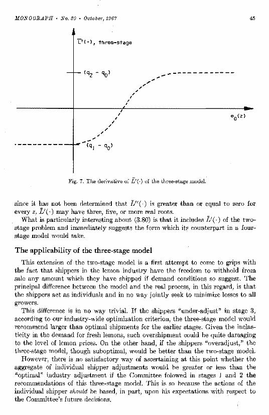
45 MONOGRAPH • No. 20 • October, 1967
L'<·>, three-stage
.... .... ------------,,.." ....
," " , , I
,, ,,/
"" " "
" ... (q, - qo>
Fig. 7. The derivative of L'(-) of the three-stage model.
since it has not been determined that L"(·) is greater than or equal to zero for every z, L'( ·) may have three, five, or more real roots.
What is particularly interesting about (3.80) is that it includes L' (·) of the twostage problem and immediately suggests the form which its counterpart in a fourstage model would take.
The applicability of the three-stage model
This extension of the two-stage model is a first attempt to come to grips with the fact that shippers in the lemon industry have the freedom to withhold from sale any amount which they have shipped if demand conditions so suggest. The principal difference between the model and the real process, in this regard, is that the shippers act as individuals and in no way jointly seek to minimize losses to all growers.
This difference is in no way trivial. If the shippers "under-adjust" in stage 3, according to our industry-wide optimization criterion, the three-stage model would recommend larger than optimal shipments for the earlier stages. Given the inelasticity in the demand for fresh lemons, such overshipment could be quite damaging to the level of lemon prices. On the other hand, if the shippers "overadjust," the three-stage model, though suboptimal, would be better than the two-stage model.
However, there is no satisfactory way of ascertaining at this point whether the aggregate of individual shipper adjustments would be greater or less than the "optimal" industry adjustment if the Committee folowed in stages 1 and 2 the recommendations of this three-stage model. This is so because the actions of the individual shipper should be based, in part, upon his expectations with respect to the Committee's future decisions.

46 Bell: Models of Commoaity Transfer
In any case, we cannot definitely say at this point which model is best for the lemon industry. But if we must err, we should err on the conservative side and utilize the rules provided by the two-stage model.
A Procedure for Applying the Two-Stage Dynamic Model.to the Lemon Industry
The multistage models rest fundamentally upon. the concept of the random variable e and u in the three-stage model and the assumption that the cost of shipping or handling is higher in later stages than in earlier stages of a given period. It is with the aid of these factors that we are able to demonstrate a rational basis for the existence of a multistage shipping system. Stated simply, the two-stage model provides a formula by which one may determine an optimal balance between the risk of overshipping in stage 1 and the higher cost of shipping in stage 2; a similar but more complicated balancing mechanism operates in the three-stage model.
As we indicated earlier, our objective has been to provide a method of determining weekly shipping quantities which minimizes the expected loss to the packinghouses, that is, which minimizes transfer cost minus gross revenue. And we mentioned that the Committee has not in the past based its weekly allocation decisions upon the criterion of profit maximization but, instead, has sought to ship as much as possible under a price constraint.
The difference between these two approaches may be great indeed. Within the framework of the Committee's present decision criteria, the existence of "two stages" is independent of considerations of risk! Essentially, the Committee makes an estimate of the maximum quantity which can be shipped at "acceptable" prices and, then, if during the week of shipment various packinghouses or sales departments are able to demonstrate that they can sell an additional amount and still obtain acceptable prices, the Committee will consider, and perhaps grant, an increase in the maximal industry shipping quantity.
The transfer functions
Given its procedure, the Committee need not be concerned with the difference in shipping cost for the two stages and, in point of fact, has not been particularly aware of any such difference.
However, we know that such a difference must exist, for otherwise, the industry woAld not announce shipments one week in advance. The major problem is that the difference, [Qi(µ) Q0(,u)], to use our standard notation, is probably nonmeasurable. The basis of this nonmeasurability is that Q1(,u) is influenced by (1) the subjective as well as the pecuniary costs associated with the altering of production and work schedules within the packinghouses and (2) the loss in sales department efficiency associated with uncertainty with respect to weekly shipping quantities. Furthermore, Q1 (,u) must measure packinghouse and sales department costs associated with levels of stage 2 shipments which have never been approached in past experience.
The nonmeasurability of Qi(,u) should not be cause for alarm, however, because the structure of the model is such that we may impute to it a logically proper and operationally useful value.
47 MONOGRAPH • No. 20 • October, 1967
First of all, the function Q0(µ)-the packing and handling cost function for stage I-has been developed, using the economic-engineering approach, by Goueli (1964). He found that the average cost of packing was a decreasing function of the rate of pack per unit of time and, also, a decreasing function of the size of plant, ceteris paribus.
However, the average cost of transfer in stage 2 may be expected to be an increasing function of the rate of pack, say, Qi(m) Co + qim2, so that we need to find some method of estimating qi.
Now, we mentioned earlier that e and [Qi(µ) - Qo(µ)] > 0 form jointly the fundamental basis of the system. For, if Qi(µ) Qo(µ), there would be no disadvantage associated with having to wait until stage 2 in order to observe the factor e*, and nothing would ever be shipped in stage I. At the other extreme, as Qi(µ) approaches infinity, stage 2 vanishes from the system.
Furthermore, as Qi(µ) grows larger, the industry's total expected loss (neglecting the cost of shipping) must decrease, ceteris paribus, because of the increased likelihood of overshipment in stage 1 and the increased reluctance to make stage 2 adjustments.
So, if the distribution of e,Qo(µ) and the revenue function may be estimated and assumed given, then the relative frequency of m > 0, the average size of m, and the level of expected total loss will be functions of q1 alone.
Hence, we may assert that the "true" value of q1 is the scalar for which the industry's seasonal marginal revenue as a function of qi is equal to the industry's marginal subjective cost of shipment over the season as a function of the number and size of stage 2 shipments (which is a function of qi). In other words, qi is a "dummy" factor which has no real meaning in itself but which must be given the smallest value for which the rewards of making it smaller in terms of total expected loss are not more than compensated by the subjective and pecuniary cost of the increased number, and size of stage 2 shipments.
To find the best qi, we simply calculate the expected optimal loss and generate the expected number and size of stage 2 shipments for the various values of q1 by direct machine simulation of the system and then allow the Committee to decide which q1 yields the most acceptable results. If, initially, the Committee's choice of qi proves in practice to be unsatisfactory, a new choice may be made at any point in the season. Given the subjective and nonmeasurable factors involved in qi, this parameter must ultimately be determined by the Committee.
Since changes in q1 have the effect of changing both the frequency and size of stage 2 shipments, it may be useful to separate q1 into two components-say, qi' and qi"- where q1' is the shipment cost which enters into the computation of e0
and determines the size of (z + m) while qi" is the shipping cost which enters only the stage I loss function and influences the size of z. In this way, we may vary the frequency of strictly positive stage 2 shipments without exaggerating the actual unit cost of shipment, q1•
The salvage value function Since the two-stage model was developed for the purpose of finding the optimal
allocation over time of some predetermined seasonal quota, the model must be so constructed and its parameters so specified that the probability is high that the
48 Bell: Models of Commodity Transfer
prescriptions of the model will lead toward the satisfaction of that goal. The simplest and most direct way of forcing the system to "unload" its supply (so as to achieve the seasonal goal) is to use the salvage value function as a "penalty" function. That is, let V(C - µ) be a nonpositive, nonincreasing function of (C - µ). Then, V(C - µ)becomes a kind of shadow price which reflects the cost of shipping the predetermined seasonal tot'al as opposed to simply minimizing short-run losses over the season without terminal constraint.
The parameters of V(C µ) may be found by the same simulation process that enables us to find the best qi" or qi'.
The price prediction equation
Although thus far we have studied the problem of statistical estimation in only the most cursory manner, it is clear that the development of an equation based upon weekly data which satisfies certain a priori assumptions with respect to the size and sign of the coefficients requires the most meticulous care. 13 Clearly, the results obtained by our preliminary analysis are unsatisfactory. However, we present them so that the reader may, if he so desires, gain from them some insight into the nature of the statistical problems involved.
A useful analysis would probably require the investigation in detail of those short-run, "shift" factors which can be shown to influence wholesaler demand for fresh lemons and perhaps there should be a separate analysis for each marketing region. But to say more about the nature of a demand study of this sort would be premature, and we hope that efforts to probe further into this question may soon be made.
It is possible that an efficient price prediction equation of the type required by the model cannot be developed because there may be no way of determining the nature of the short-run shifts which influence the relationship between price and the quantity sold.
The minimum level of efficiency which the price prediction equation must display is difficult to define without logical circularity. If it may be assumed that the model is one which, given some price prediction equation, is capable of improving the operation of the process, then an equation which displays the lower bound of efficiency may be defined as one which produces results from the model which are no better than those which the industry obtains without the use of the model. Hence, there may be a set of efficient price prediction equations. It should be enlphasized that this criterion of efficiency does not require that the forecast derived from an efficient equation possess a smaller error on the average than forecasts which the industry may develop through the use of experts who carefully examine factors from week to week without the use of equations.
Concluding remarks In the two- and three-stage models, the marketing firm was assumed to be
monopolist which possesses little or no control over the amount that it had to sell
1a For instance, if the equation includes lagged prices, their coefficients should be positive and less than unity; if temperature is used as a factor, its coefficient should be positive; if the quantity sold is a factor, its coefficient should be negative and in or near the set of numbers for which demand would be inelastic, and so on.

49 MONOGRAPH • No. 20 • October, 1967
within its time horizon. It was further assumed that the commodity in question was indefinitely storable or at least was capable of surviving storage over a number of periods.
This set of assumptions tends to restrict the applicability of the multistage models to a relatively small number of agricultural industries and, of those industries, the California-Arizona lemon industry may be the only one which presently possesses the required structural and institutional arrangements.
However, the two- and three-stage models possess considerable flexibility. The most fundamental elements of this flexibility stem from the possibility of making meaningful alterations in the dummy parameters, q1" and v, but an investigator may also make successive improvements in other specifications, introduce additional specifications, and thereby adapt the model more completely to a particular problem.
At the cost of greatly increasing the computer time necessary for the problem, it would be possible to introduce probability distributions for the weekly harvest estimates and the x", the predictors of x'. Moreover, the harvest pattern, the dt-h
could be artificially but systematically distorted so as to minimize administrative difficulties which may arise when consideration of only the overall harvest pattern tends to greatly disadvantage some producers relative to others.
In these and other ways, it should be possible to adapt the multistage models to real processes so that they may prove to be useful tools with which to analyze and improve the operation of a number of commodity transfer processes.
ACKNOWLEDGMENTS
The author should like to express appreciation to George M. Kuznets, Professor of Agricultural Economics, Berkeley, for his invaluable suggestions and encouragement; to the reviewers, especially Irving J. Hoch; and to the Department of Agricultural Economics for financial assistance.
BIBLIOGRAPHY
ALTSCHUL, E. B., and E. BISER 1948. The validity of unique mathematical models in science. Philosophy of Science (15):
265-81. ARROW, KENNETH J.
1951A. Alternative approaches to the theory of choice in risk-taking situations. Econometrica, 19(4); 404--37.
1951n. Social choice and individual values. Cowles Commission for Research in Economics Monograph No. 12. New York: Jqhn Wiley & Sons, Inc.
ARROW, KENNETH J., THEODORE HARRIS, and JACOB MARSCHAK 1951. Optimal invent-Ory policy. Econometrica, 19(3) :250-72.
ARRow, KENNETH J., SAMUEL KARLIN, and HERBERT ScARF 1958. Studies in the mathematical theory of inventory and production. Stanford University
Press, California. BADIER, P., G. NAHoN, and B. RoY
1963. Stockage et exportation des cereales francaises (example d'application de la programmation dynamique). Metra, 2(1).
BAUMOL, WILLIAM J. 1961. Economic theory and operations analysis. Englewood Cliffs, N. J.: Prentice-Hall, Inc.
50 Bell: Models of Commodity Transfer
BLACK, DUNCAN 1948A. The decisions of a committee using a special majority. Econometrica, 16(3) :245-61. 1948B. The elasticity of committee decisions with an altering size of majority. Econometrica,
16(3) :262-70. 1948c. On the rationale of group decision-making. Jour. of Political Economy, 56(1) :22--34.
BRENNAN, MICHAEL J. 1959. A model of seasonal inventories. Econometrica, 27 (2) :228-44.
BROWN, R. G. 1962. Smoothing, forecasting and prediction of discrete time series. Englewood, N. J.: Prentice
Hall, Inc. CARTER, C. F., G. P. MEREDITH, and G. L. S. SHACKLE
1957. Uncertainty and business decisions. University Press of Liverpool, England. CHA:aNEs, A., and W. W. CooPER
1961. Management models and industrial applications of linear programming, I. New York: John Wiley & Sons, Inc.
CHERNOFF, HEIUfAN 1954. Rational selection of decision functions. Econometrica, 22(4) :422-43.
CHUltCHMAN, c. w. 1961. Prediction and optimal decision. Englewood, N. J.: Prentice-Hall, Inc.
CHURCHMAN, C. W., R. L. AcKOFF, and E. L. AaNOFF 1957. Introduction to operations research. New York: John Wiley & Sons, Inc.
CoOMBS, C. H., and DAVID BEAltDSLEE 1954. On decision-making under uncertainty. In: Thrall, R. M., et al., Decision processes.
Chapter 17. New York: John Wiley & Sons, Inc. DANIEL, K. H.
1961. A delivery-lag inventory model with emergency. Institute of Engineering Research ORC 172-13. University of California, Berkeley.
DORFMAN, ROBERT 1951. Application of linear programming to the theory of the firm. University of California
Press, Berkeley. DORFMAN, ROBERT, PAUL A. SAMUELSON, and RoBEltT M. Soww
1958. Linear programming and economic analysis. New York: McGraw-Hill Book Co., Inc. FELLE:a, W.
1957. An introduction to probability theory and it.'l applications, I. New York: John Wiley & Sons, Inc.
FREUND, R. J. 1956. The introduction of risk into a programming model. Econometrica, 24(3) :253-63.
Goon, I. J. 1952. Rational decisions. Jour. of the Royal Statistical Society, Series B (Methodological),
14(1) :107-14. GouELI, AHMED A. M.
1964. Economic planning of production and marketing facilities. Unpub. Ph.D. dissertation. University of California, Berkeley.
HADLEY, GEORGE and T. M. WHITIN 1963. Analysis of inventory systems. Englewood Cliffs, N. J.: Prentice-Hall, Inc.
Hoos, SrnNEY and GEORGE M. KuzNETS 1962. Impacts of lemon products imports on domestic lemon markets. Giannini Foundation j Res. Rept. 254. University of California, Berkeley.
Hoos, S., and R. E. SELTZER 1952. Lemons and lemon products, changing economic relationships. California Agric. Expt.
Sta. Bull. 729. HURIWICZ, L.
1946. Theory of the firm and of investment. Econometrica, 14(2) :109-36. JEWELL, WILLIAM s.
1961. A linear risk model. Operational Research Quarterly, 12(4):209-20. KA:aLIN, SAMUEL
1959. Mathematical methods and theory in games, programming, and economics, I. Reading, Mass.: Addison-Wesley Publishing Company, Inc.
KUZNETS, GEORGE M. 1963. Theory and quantitative research. Jour. of Farm Economics, 45(5) :1393-1400.
KuzNETS, GEORGE M., and S. Hoos 1962. Impacts of lemon products on domestic lemon markets. Giannini Foundation Res. Rept.
254, University of California, Berkeley.
51 MONOGRAPH • No. 20 • October, 196'?"
LEMON ADMINISTRATIVE COMMITTEE 1960-1964. Annual Report. Los Angeles, California. 1958-1962. Weekly Newsletter. Los Angeles, California.
LUTZ, F., and V. LUTZ 1951. Theory of investment of the firm. Princeton University Press, New Jersey.
MARKOWITZ, H. M. 1960. Portfolio selection. New York: John Wiley & Sons, Inc.
MARSCHACK, JACOB 1950. Rational behavior, uncertain prospects, and measurable utility. Econometrica, 18(2):
111-41. MILLS, E. S.
1962. Price, output and inventory policy. New York: John Wiley & Sons, Inc. MODIGLIANI, FRANCO and FRANZE. HOHN
1955. Production planning over time and the nature of the expectation and planning horizon. Econometrica, 23(1) :46--66.
MULLER, R. H. 1944. Verification of short range weather forecasts. American Meteorological Soc., 25.
NASH, J. F. 1950. The bargaining problem. Econometrica, 18(2) :155-62.
01, WALTER Y. 1961. The desirability of price instability under perfect competition. Econometrica, 29(1):
58-64. SAATY, T. L.
1961 Elements of queueing theory. New York: McGraw-Hill Book Co., Inc. SIMON, HERBERT A.
1956. Dynainic programining under uncertainty with a quadratic criterion function. Econometrica, 24(1) :74--81.
SMITHIES, A. 1939. The maxiinization of profits over time with changing cost and demand functions. Econ
ometrica, 7(4):312-18. SUNKIST GROWERS
1964. 1964 supplement, statistical information on the citrus fruit industry. Los Angeles, California.
THRALL, R. M., C.H. CooMBS, and R. L. DAVIS . 1954. Decision processes. New York: John Wiley & Sons, Inc.
TINTNER, GERHARD 1941A. The theory of choice under subjective risk and uncertainty. Econometrica, 9(3 & 4):
298-304. 1941B. The pure theory of production under technological risk and uncertainty. Econometrica,
9(3 & 4):305-12. TISDELL, CLEM
1963. Uncertainty, instability, expected profit. Econometrica, 31(1-2) :243-47. U. S. WEATHER BUREAU
1957-1959. Climatological information, by states. Washington, D.C. 1961. Verification of the Weather Bureau's 30 day outlooks. Tech. Paper 39. Washington, D.C.
VAJDA, s.. 1961. Mathematical programming. Reading, Mass.: Addison-Wesley Publishing Company, Inc.
VAUGH, FREDERICK V., EDGAR L. BURTIS, and A. F. WOLF 1936. The controlled distribution of a crop among independent markets. Quarterly Jour. of
Econoinics, 51(1) :1-41.
2m-10, 67 (H3473) JF
GIANNINI FOUNDATION MONOGRAPHS TO DATE
The first 17 titles in the Giannini Foundation Monograph Series were published in Hilgardia and are listed below. Numbers 18 et seq. are published in the present format. See hack cover for information on obtaining copies.
No. L Major Economic Forces Affecting Agriculture, with Particular Reference to California, by S. V. Ciriacy-Wantrup. (Hilgardia, Volume 18, Number 1, December, 1947) 76 pages.
No. 2. Characteristics of Demand for California Plums, by Jerry Foytik. (Hilgardia, Volume 20, Number 20, April, 1951) 121 pages.
No. 3. Pricing Efficiency in the Manufactured Dairy Products Industry, by James B. Hassler. (Hilgardia, Volume 22, Number 8, August, 1953) 100 pages.
No. 4. Statistical Analysis of Supply Response in Late Spring Potatoes in California, by Chester 0. McCorkle, Jr., and Yair Mundlak. (Hilgardia, Volume 24, Number 16, April, 1956) 39 pages.
No. 5. Economic Efficiency in Plant Operations With Special Reference to the Marketing of California Pears, by B. C. French, L. L. Sammet, and R. G. Bressler. (Hilgardia, Volume 24, Number 19, July, 1956) 179 pages. (Out of print-available on microfilm only.)
No. 6. Soil Variables for Use in Economic Analysis, by David Weeks and J. Herbert Snyder. (Hilgardia, Volume 26, Number 11, April, 1957) 24 pages.
No. 7. Economies of Scale for Evaporated Milk Plants in California, by James N. Boles. (Hilgardia, Volume 27, Number 21, October, 1958) 102 pages.
No. 8. Income, Price, and Yield Variability for Principal California Crops and Cropping Systems, by H. 0. Carter and G. W. Dean. (Hilgardia, Volume 30, Number 6, October, 1960) 44 pages.
No. 9. The Impact of Irrigation on Farm Output in California, by Vernon W. Ruttan. (Hilgardia, Volume 31, Number 4, July, 1961) 43 pages.
No. ID. Interregional Competition in the Frozen Strawberry Industry, by C. C. Dennis and L. L. Sammet. (Hilgardia, Volume 31, Number 15, December, 1961) 113 pages.
No. 11. Econometric Analysis of the Market for California Early Potatoes, by Pinhas Zusman. (Hilgardia, Volume 33, Number 11, December, 1962) 120 pages.
No.12. Orderly Marketing for California' Avocados, by Stephen H. Sosnick. (Hilgardia, Volume 33, Number 14, December, 1962) 70 pages.
No. 13. Regional Location of Cattle Feeding-A Spatial Equilibrium Analysis, by G. A. King and L. F. Schrader. (Hilgardia, Volume 34, Number IO, July, 1963) 86 pages.
No.14. Optimal Cooperative Pools for California Avocados, by Stephen H. Sosnick. (Hilgardia, Volume 35, Number 4, September, 1963) 38 pages.
No. IS. The Economics of Conjunctive Use of Ground and Surface Water, by Oscar R. Burt. (Hilgardia, Volume 36, Number 2, December, 1964) Bl pages.
No. 16. Size and Location Factors Affecting California's Beef Slaughtering Plants, by S. H. Logan and G. A. King. (Hilgardia, Volume 36, Number 4, December, 1964) 50 pages.
No. 17. Interregional Competition in the United States Turkey Industry, by D. Lee Bawden, H. O. Carter, and G. W. Dean. (Hilgardia, Volume 37, Number 13, June, 1966) 95 pages.
No. IB. World Trade in Fresh Oranges: An Analysis of the Effect of European Economic Com· munity Tariff Policies, by Gerald W. Dean and Norman R. Collins. (Giannini Foundation Monograph, January, 1967) 70 pages.
No.19. Conditional Projections of California Economic Growth, by Ivan M. Lee. (Giannini Foundation Monograph, February, 1967) 120 pages.

GIANNINI FOUNDATION MONOGRAPH SERIES
What it is
The Giannini Foundation Monograph Series is comprised of technical research reports relating to the economics of agriculture. The series, introduced in 1967, is published by the California Agricultural Experiment Station. Similar technical economic research studies formerly were published in Hilgardia.
Each Monograph is a separate report of research undertaken in the California Experiment Station by staff members of the Department of Agricultural Economics and the Giannini Foundation of Agricultural Economics in the University of California. Topics covered range from analyses of farm and processing firms to broader problems of interregional resource use and public policy.
The Monographs are written in technical terms with professional economists as the intended audience. No attempt is made to reduce the writing to terms understandable to the layman. Each Monograph carries an abstract on the inside front cover.
Monographs are published at irregular intervals as research is completed and reported.
How to obtain copies
In general, copies will be sent free on request to individuals or organizations. The limit to California residents is 20 titles; the limit to non· residents is 10. There is no distribution through agencies or stores.
A list of available Monographs in the series is published annually and may he obtained by writing to Agricultural Publications (address below). The list also explains how some out-of-print issues, including reports that formerly appeared in Hilgardia, may be obtained on microfilm or as record prints. To obtain the Giannini Foundation Monograph Series regularly, certain minimum qualifications must be met:
As a gift. Some libraries, educational institutions, or agricultural experiment stations may receive Monographs as issued where there is
J a definite need for the material and it will be made available to a con· siderable number of interested economists. Address requests to Agri· cultural Publications. Please give particulars.
As an exchange for similar research material. Address requests to Librarian, Giannini Foundation of Agricultural Economics, University of California, Berkeley, California 94720.
With the exception of communications about exchange agreements (see above), address all correspondence concerning the Giannini Foundation Monograph Series to:
Agricultural Publications University Hall University of California Berkeley, California 94720