Predicting Pattern Tooling and Casting Dimensions for - OSTI
Upload
theijesCategory
view
36download
1
The International Journal Of Engineering And Science (IJES)
|| Volume || 4 || Issue || 4 || Pages || PP.23-36|| 2015 ||
ISSN (e): 2319 – 1813 ISSN (p): 2319 – 1805
www.theijes.com The IJES Page 23
Models for predicting body dimensions needed for furniture
design of junior secondary school one to two students.
1OladapoS.O,
2AkanbiO.G
1Department of Industrial and Production EngineeringUniversity of Ibadan, Nigeria.
2Department of Industrial and Production EngineeringUniversity of Ibadan, Nigeria.
-------------------------------------------------------------ABSTRACT-------------------------------------------------------
Purpose – The purpose of this study was to develop some models that will make use of easy-to-measure
students’ body dimensions to predict difficult, time-consuming and energy-sharping anthropometric dimensions
needed for ergonomic school furniture design for junior secondary school one to two
students.Design/methodology/approach – A total of 160 students aged 11 to 13 years were randomly selected
from eight public secondary schools in Ogbomoso, South West Nigeria. All the dimensions were analyzed using
Microsoft excel sheet 2010 and Design Expert version 6.0.8.The models with no/non-significant lack of fit and
highest coefficient of determinations were selected as the best models for the required predictions.Findings –
The study led to the development of 12 models that utilyzed easy-to-measure dimensions for estimating
necessary anthropometric dimensions for the design of school furniture. The results of the study revealed that
two-third of the anthropometric dimensions exhibited non-linear models.Originality/value – The furniture
industry would find in these models economical, adequate and effective prediction tools.
KEY WORDS:anthropometric dimensions, models, furniture industry.
-------------------------------------------------------------------------------------------------------------------------------------- Date of Submission: 12-March-2015 Date of Accepted: 20-April-2015
--------------------------------------------------------------------------------------------------------------------------------------
I. INTRODUCTION
Furniture has an important role in the maintenance of good sitting posture. Using furniture that
promotes proper posture is more important to children than adult because it is at this young age that sitting
habits are formed (Reis et al., 2012). Bad sitting habits acquired in childhood and/or adolescence are very
difficult to change later in adulthood (Yeats, 1997). Bad sitting habits are not unconnected with bad furniture
design.Bad design of furniture may lead to health and learning problems. Therefore, design of furniture with
proper dimensions is critical to encourage appropriate posture (Straker et al., 2010).
This necessitated the need for complete anthropometric data for each country (Garcia-Acosta and
Lange-Morales, 2007) and based on anthropometric data obtained from the intended users, every country can
design fitting furniture for school children (Molenbroek and Ramaekers, 1996; Oyewole et al., 2010) instead of
a one-size-fits-all philosophy that has been adopted in the industry (Parcells et al., 1999; Adewole and
Olorunnisola, 2010; Niekerk et al., 2013). This will require anthropometric data of the targeted population
which are not ease-to-measure and time consuming. Furthermore, creating anthropometric databases usually
requires considerable resources in terms of workforce, equipment, and funds.It is unlikely that the furniture
industry will be able to rise to these challenges without better tools that can help it to achieve the desired
furniture at minimum labour and time. Hence, the development of some models that will effectively make use of
ease-to-measure dimensions to predict the difficult-to-measure ones needed for the design of school furniture is
required. According to Ismaila et al., (2014), anthropometric regression models have been used in the
development of ergonomic designs of various products and workstations. In fact, You and Ryu (2005) stated
that most of the linear anthropometric regression models use only stature and/or weight to estimate body
dimensions which resulted in unsatisfactory prediction for an anthropometric variable with low correlation (r)
and low coefficient of determination (R2).
Low coefficient of determination is an indication that the model is under fitted, that is, variable(s) that
are really useful is/are not included in the model. This may be due to the fact that most researchers had
concentrated on the economic reason while they had lost sight of adequacy and accuracy of the model.
Therefore, the aim of this study was to develop some models that will make use of easy-to-measure students’
body dimensions to predict difficult, time-consuming and energy-sharping anthropometric dimensions needed
for ergonomic school furniture design.

Models For Predicting Body Dimensions…
www.theijes.com The IJES Page 24
II. METHODOLOGY
A total of 160 students (81 male, 79 female) of those who volunteered to participate in the study were
randomly selected from junior secondary school one to two (J.S.S. 1-J.S.S. 2) in Ogbomoso, Oyo state Nigeria.
They had no physical disabilities and had not participated in such previous study. Their age range is between 11
and 13years. The appropriateness of the sample size was verified using GPower 3.1 software version. The
significant level and effect size that were used are 0.05 and 0.1 (small effect) respectively. The result of the
analysis; sample size 160, number of predictors 4; returned a Power = 0.9753871. Since a power of 0.8 or
greater is considered powerful conventionally, then the result of power analysis of 0.9999993 is adequately
sufficient. However, if too many observations are used, even a trivial effect will be mistakenly detected as a
significant one (High, 2000). By contrast, if too few observations are used, a hypothesis test will be weak and
less convincing. Accordingly, there may be little chance to detect a meaningful effect even when it exists there.
This led to a priori analysis to determine whether the sample size was actually not below or above the needed
number of observation. A power of 95% was employed and the analysis returned a sample size of 132 as
adequate. This justified the sample size of 160 used by the researchers as the resulted difference meant more
power for the research. The demographic stratification parameter employed were levels in schools and
gender. Jeong andPark (1990) had stated that Sex difference in anthropometry is significant for school furniture
design. Measurements were carried out on the right-hand side of the participating students, to the nearest
centimetre while the subjects were wearing light clothing and barefooted.The user’s dimensions were taken and
defined as presented below. They were taken with the use of anthropometer (Model 01290. Lafayette instrument
company, Lafayette Indiana), tape measure, normal chair used by students in school, flat wooden pieces (used as
foot rest to accommodate students of different heights) and a perpendicular wooden angle. The perpendicular
wooden angle was used to fix the elbow at 900 as required for the measurements.
Stature (ST): Measured as vertical distance from floor to crown of head in standing position while the
subject looks straight ahead.
Waist Height, Standing (WH): Measured as vertical distance from floor to the highest point on the
waist in standing position.
Shoulder – grip Length (SL): Measured as horizontal distance from the shoulder to the tip of the
longest finger in standing position.
Lower –arm length (LL): Measured as the horizontal distance from the elbow, when flexed at 900, to
the tip of the longest finger in standing position.
Shoulder breadth (SB): Measured as the maximum horizontal distance across the shoulder in sitting
position.
Knee Height (KH): Measured as vertical distance from the floor or footrest to the uppermost point on
the knee in sitting position with knee flexed at 900.
Elbow Rest Height (EH): Measured as vertical distance from the sitting surface to the bottom of the
right elbow while the elbow was flexed at 900 and shoulder was flexed at 0
0.
Popliteal Height (P): Measured as the vertical distance from the floor or the footrest to the underside of
the thigh immediately behind the knee in the sitting position with knee flexed at 900.
Shoulder Height (SHH): Measured as the vertical distance from the sitting surface to the top of the
shoulder at the acromion position.
Buttock-Popliteal Length (BPL): Measured as the horizontal distance from the rear surface of the
buttock to the internal surface of the knee, or popliteal surface, with the knee flexed at 900.
Hip Width (HW): Measured as maximum horizontal distance across the hips in the sitting position.
The measurement was done thrice and the mean values were used as representing the true values. The
measured data were analyzed using Microsoft excel sheet 2010 and Design Expert version 6.0.8. Descriptive
statistics were reported (mean, minimum, maximum and 5th, 50th and 95th percentiles) to describe the
anthropometric dimensions of subjects.
The dimensions were divided into dependent and independent variables. The dependent variables were the
dimensions needed for school furniture design. This is because they are easy-to-measure and they are KH, EH,
SHH, P, BPL and HW (Parcells, et al., 1999; Agha, et al., 2012). The independent variables were ST, WH, SL,
LL, and SB because they are not easy-to-measure.Second order polynomial response surface model (equation
twenty) was fitted to each of the response variable.
𝑌 = 𝛽° + 𝛽𝑖𝑥𝑖 + 𝛽𝑖𝑗 𝑥𝑖𝑥𝑗 +
𝑘
𝑖<𝑗
𝛽𝑖𝑖
𝑘
𝑖=1
𝑘
𝑖=1
𝑥𝑖2 + 𝜀 …………… (1)
Data were modeled by multiple regression analysis and the statistical significance of the terms was
examined by analysis of variance for each response. The statistical analysis of the data and three dimensional
plotting were performed using Design Expert Software (Stat-Ease 2002). The adequacy of regression model was
checked by lack-of fit test, R2, AdjR
2, Pre R
2, Adeq Precision and F-test (Montgomery 2001). The significance

Models For Predicting Body Dimensions…
www.theijes.com The IJES Page 25
of F value was judged at 95% confidence level. The regression coefficients were then used to make statistical
calculation to generate three-dimensional plots from the regression model.
III. RESULTS. The anthropometric dimensions of the students are presented in tables 1-2.
Table 1: The Mean, Minimum, Maximum and 5th, 50th And 95th Percentiles of J.S.S. 1-J.S.S. 2 Male for each
Anthropometric Measurement (cm).
Table 2The Mean, Minimum, Maximum and 5th, 50th And 95th Percentiles of J.S.S. 1-J.S.S. 2 Female for each
Anthropometric Measurement (cm).
Mean Min Max 5th Percentile 50th Percentile 95th Percentile
ST 152.93 134.00 170.80 142.62 153.40 164.05
WH 89.29 51.70 102.00 80.93 90.00 100.00
SL 70.39 58.70 92.80 64.00 70.00 78.26
LL 44.47 37.70 51.20 40.30 44.50 48.50
SB 26.12 20.10 33.90 22.18 26.20 30.17
KH 49.86 43.00 55.50 46.00 49.80 54.03
EH 17.10 12.00 22.00 13.10 17.00 20.11
P 40.10 34.00 45.10 36.45 40.00 44.25
SHH 47.79 42.00 57.00 42.60 47.50 53.50
BPL 45.98 39.80 51.60 42.07 45.60 50.21
HW 28.46 23.00 34.60 24.61 28.60 31.82
3.1 Models Presentation and Analysis for J.S.S.1-J.S.S.2 Male.
Data Analysis for Response 1: Knee Height
Quadratic model is suggested by the design program for this response to test for its adequacy and to
describe its variation with independent variables. From ANOVA test in table 3, the Model F-value of 154.96
implies the model is significant. There is only a 0.01% chance that a "Model F-Value" this large could occur
due to noise.
Mean Min Max 5th Percentile 50th Percentile
95th
Percentile
ST 147.47 132.80 174.00 135.50 145.90 162.30
WH 87.31 74.10 106.70 75.89 87.35 96.58
SL 67.55 56.40 82.00 60.00 67.00 75.50
LL 42.51 16.50 52.00 37.90 42.50 47.80
SB 25.60 18.10 44.90 20.60 25.60 29.50
KH 48.26 42.40 58.40 43.00 48.20 53.70
EH 16.06 8.20 21.00 12.20 16.20 19.40
P 39.02 33.00 47.30 35.00 38.80 44.10
SHH 45.16 36.30 54.70 39.20 44.80 52.10
BPL 42.62 31.60 51.00 37.30 43.00 49.00
HW 26.10 21.70 32.00 22.50 26.10 30.70
Models For Predicting Body Dimensions…
www.theijes.com The IJES Page 26
Table 3: ANOVA test for KH
Source Sum of
squares
Df Mean square F value P-value
Prob> F
Significant
Model 779.66 5 155.93 154.96 < 0.0001
A 59.43 1 59.43 59.06 < 0.0001
B 9.847*10-5 1 9.847 *10-5 9.785 *10-5 0.9921
A2 12.92 1 12.92 12.84 0.0006
B2 6.50 1 6.50 6.46 0.0131
AB 14.26 1 14.26 14.17 0.0003
Residual 75.47 75 1.01
Cor Total 855.13 80
Values of "Prob> F" less than 0.0500 indicate model terms are significant. In this case A, A2, B2, and
AB are significant model terms. Values greater than 0.1000 indicate the model terms are not significant.
The non-appearance of "Lack of Fit F-value" implies that the model perfectly (100%) fit relative to the
pure error.
Table 4: Post ANOVA Statistics for KH
Std. Dev. 1.00 R-Squared 0.9117
Mean 48.42 Adj R-Squared 0.9059
C.V. 2.07 Pred R-Squared 0.8871
PRESS 96.59 Adeq Precision 56.780
From table 4, the "Pred R-Squared" of 0.8871 is in reasonable agreement with the "Adj R-Squared" of 0.9059.
"Adeq Precision" measures the signal to noise ratio. A ratio greater than 4 is desirable. The ratio of 56.780
indicates an adequate signal. This model can be used to navigate the design space (Montgomery 2001).
In the same manner, other responses were analyzed and the resulted is presented in table 5.
Table 5: Design Summary for J.S.S.1-J.S.S.2 Male
Study type: response surface Experiments: 232
Initial design: historical data Blocks: no blocks
Design model: quadratic
response name Units obs minimum Maximum trans Model
Y1 KH Cm 81 42.40 58.40 None Quadratic
Y2 EH Cm 81 15.04 18.17 None Quadratic
Y3 P Cm 81 33.00 46.02 None Linear
Y4 SHH Cm 81 39.58 53.15 None Quadratic
Y5 BPL Cm 81 37.30 49.82 None Quadratic
Y6 HW Cm 81 22.78 30.65 None Quadratic
3.1.1 Model Equations for J.S.S.1-J.S.S.2 Male
Model equations are given in terms of coded factors and actual factors. Coded factors indicate when the
minimum and maximum values of the factors are represented by -1 and +1 respectively instead of their actual
values.
Response 1: Knee Height
The model in terms of coded factors is given by:
KH = +50.28 +7.52*A +0.010*B +5.64*A2 +3.88*B2 -10.02*A*B……. (2)
The model in terms of actual factors is given by:
KH = +16.92952 -1.08033*ST +2.54894*SL +0.018283*ST2 +0.023711*SL2 -
0.038004*ST*SL……………………………………………… (3)
Response 2: Elbow Height
The model in terms of coded factors is given by:
EH = +16.62 +2.33*A -0.93*B +0.40*A2 +0.16*B2 -0.60*A*B………….. (4)
The model in terms of actual factors is given by:
EH = +6.91606 -0.016823*ST +0.13924*SL +9.34441*10-4*ST2 +9.74561*10-4*SL2 -2.26186*10-3*ST*SL
…………………………………… (5)
Response 3: Popliteal Height
The model in terms of coded factors is given by:

Models For Predicting Body Dimensions…
www.theijes.com The IJES Page 27
P = +40.33 +3.33*A +3.09*B ……………………………………….………….. (6)
The model in terms of actual factors is given by:
P = -1.13642 +0.16147*ST +0.24131*SL ………………………………….. (7)
Response 4: Shoulder Height
The model in terms of coded factors is given by:
SHH = +47.36 +11.30*A -5.27*B +9.12*A2 +9.22*B2 -19.82*A*B…….. (8)
The model in terms of actual factors is given by:
SHH = -31.08688 -0.84157*ST +3.32834*SL +0.021482*ST2 +0.056273*SL2 -
0.075152*ST*SL……………………………………………... (9)
Response 5: Buttock Popliteal Length
The model in terms of coded factors is given by:
BPL = +44.06 +5.65*A +0.57*B +4.92*A2 +4.52*B2 -9.59*A*B………… (10)
The model in terms of actual factors is given by:
BPL = +17.82466 -0.76791*ST +1.80720*SL +0.011599*ST2 +0.027568*SL2 -
0.036361*ST*SL……………………………………………. (11)
Response 6: Hip Width
The model in terms of coded factors is given by:
HW = +26.85 +2.24*A +1.62*B +1.01*A2 +1.14*B2 -2.11*A*B………. (12)
The model in terms of actual factors is given by:
HW = +6.36460 -0.072009*ST +0.38488*SL +2.38982*10-3*ST2 +6.98325*10-3*SL2 -7.98611*10-3*ST*SL
…………………………………. (13)
3.1.2 Diagnostic Test-Normal Plots of Residuals and Predicted vs Actual Plots for J.S.S.1-J.S.S.2 Male
Normal plots of residuals and predicted vs actual Plots do show how precisely the responses are
modeled. If all the points line up nicely and the deviation of points of the responses from normality is
insignificant, then the model is a very good one.
Take KH for example, from figures 1-2 below, it is clearly observed that the developed models are very
good models.
Figure 1: Normal plot of residuals for KH
Figure 2: Predicted vs actual for KH
DESIGN-EXPERT PlotKH
Studentized Residuals
Norma
l % Pro
bability
Normal Plot of Residuals
-2.14 -0.88 0.39 1.65 2.91
1
5
10
20
30
50
70
80
90
95
99
DESIGN-EXPERT PlotKH
Actual
Predic
ted
Predicted vs. Actual
42.25
46.29
50.33
54.36
58.40
42.25 46.29 50.33 54.36 58.40
Models For Predicting Body Dimensions…
www.theijes.com The IJES Page 28
3.1.3 Response Surface Plots Analysis for J.S.S.1-J.S.S.2 Male
To aid visualization of variation in responses with respect to independent variables, series of three
dimensional response surfaces were drawn using Design Expert Software (Stat-Ease 2002).
Response 1: Knee Height
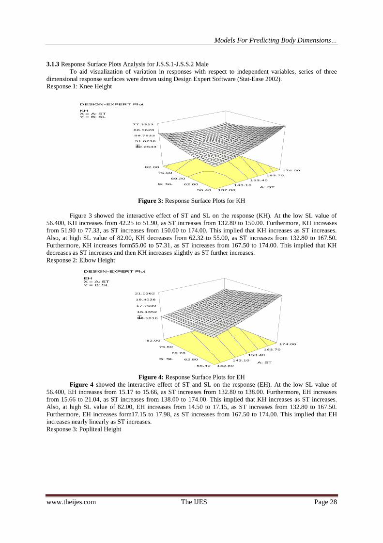
Figure 3: Response Surface Plots for KH
Figure 3 showed the interactive effect of ST and SL on the response (KH). At the low SL value of
56.400, KH increases from 42.25 to 51.90, as ST increases from 132.80 to 150.00. Furthermore, KH increases
from 51.90 to 77.33, as ST increases from 150.00 to 174.00. This implied that KH increases as ST increases.
Also, at high SL value of 82.00, KH decreases from 62.32 to 55.00, as ST increases from 132.80 to 167.50.
Furthermore, KH increases form55.00 to 57.31, as ST increases from 167.50 to 174.00. This implied that KH
decreases as ST increases and then KH increases slightly as ST further increases.
Response 2: Elbow Height
Figure 4: Response Surface Plots for EH
Figure 4 showed the interactive effect of ST and SL on the response (EH). At the low SL value of
56.400, EH increases from 15.17 to 15.66, as ST increases from 132.80 to 138.00. Furthermore, EH increases
from 15.66 to 21.04, as ST increases from 138.00 to 174.00. This implied that KH increases as ST increases.
Also, at high SL value of 82.00, EH increases from 14.50 to 17.15, as ST increases from 132.80 to 167.50.
Furthermore, EH increases form17.15 to 17.98, as ST increases from 167.50 to 174.00. This implied that EH
increases nearly linearly as ST increases.
Response 3: Popliteal Height
DESIGN-EXPERT Plot
KHX = A: STY = B: SL
42.2543
51.0238
59.7933
68.5628
77.3323
KH
132.80
143.10
153.40
163.70
174.00
56.40
62.80
69.20
75.60
82.00
A: ST
B: SL
DESIGN-EXPERT Plot
EHX = A: STY = B: SL
14.5016
16.1352
17.7689
19.4026
21.0362
EH
132.80
143.10
153.40
163.70
174.00
56.40
62.80
69.20
75.60
82.00
A: ST
B: SL

Models For Predicting Body Dimensions…
www.theijes.com The IJES Page 29
Figure 5: Response Surface Plots for P
Figure 5 showed the interactive effect of ST and SL on the response (P). At the low SL value of
56.400, P increases from 33.92 to 35.00, as ST increases from 132.80 to 140.00. Furthermore, P increases from
35.00 to 40.57, as ST increases from 140.00 to 174.00. This implied that P increases as ST increases. Also, at
high SL value of 82.00, P increases from 40.09 to 46.00, as ST increases from 132.80 to 167.50. Furthermore, P
increases from40.09 to 46.75, as ST increases from 167.50 to 174.00. This implied that P increases linearly as
ST increases.
Response 4: Shoulder Height
Figure 6: Response Surface Plots for SHH
Figure 6 showed the interactive effect of ST and SL on the response (SHH). At the low SL value of
56.400, SHH increases from 39.85 to 49.57, as ST increases from 132.80 to 141.85. Furthermore, SHH
increases from 49.57 to 102.09, as ST increases from 141.85 to 174.00. This implied that SHH increases as ST
increases. Also, at high SL value of 82.00, SHH decreases from 68.94 to 50.00, as ST increases from 132.80 to
167.50. Furthermore, SHH increases slightly from 50.00 to 51.91, as ST increases from 167.50 to 174.00. This
implied that SHH decreases as ST increases and then KH increases slightly as ST further increases.
.Response 5: Buttock Popliteal Length
DESIGN-EXPERT Plot
PX = A: STY = B: SL
33.9167
37.1243
40.3318
43.5393
46.7469
P
132.80
143.10
153.40
163.70
174.00
56.40
62.80
69.20
75.60
82.00
A: ST
B: SL
DESIGN-EXPERT Plot
SHHX = A: STY = B: SL
39.4401
55.102
70.7639
86.4258
102.088
SHH
132.80
143.10
153.40
163.70
174.00
56.40
62.80
69.20
75.60
82.00
A: ST
B: SL
Models For Predicting Body Dimensions…
www.theijes.com The IJES Page 30
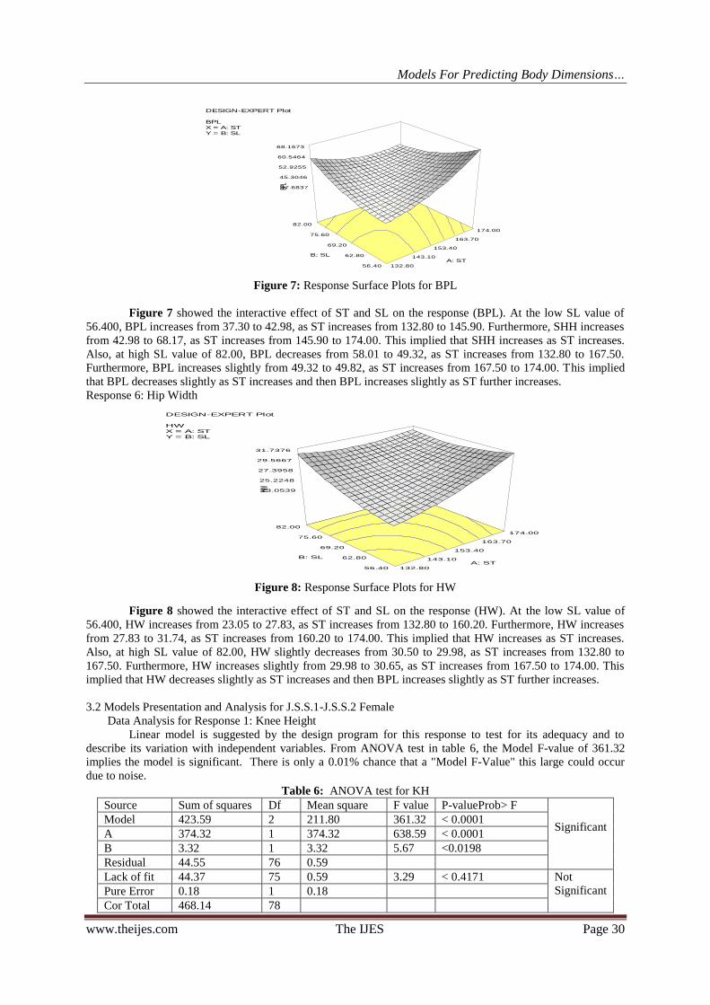
Figure 7: Response Surface Plots for BPL
Figure 7 showed the interactive effect of ST and SL on the response (BPL). At the low SL value of
56.400, BPL increases from 37.30 to 42.98, as ST increases from 132.80 to 145.90. Furthermore, SHH increases
from 42.98 to 68.17, as ST increases from 145.90 to 174.00. This implied that SHH increases as ST increases.
Also, at high SL value of 82.00, BPL decreases from 58.01 to 49.32, as ST increases from 132.80 to 167.50.
Furthermore, BPL increases slightly from 49.32 to 49.82, as ST increases from 167.50 to 174.00. This implied
that BPL decreases slightly as ST increases and then BPL increases slightly as ST further increases.
Response 6: Hip Width
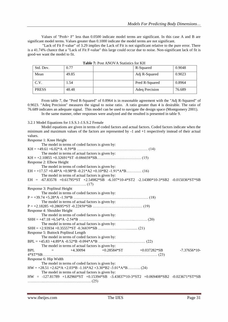
Figure 8: Response Surface Plots for HW
Figure 8 showed the interactive effect of ST and SL on the response (HW). At the low SL value of
56.400, HW increases from 23.05 to 27.83, as ST increases from 132.80 to 160.20. Furthermore, HW increases
from 27.83 to 31.74, as ST increases from 160.20 to 174.00. This implied that HW increases as ST increases.
Also, at high SL value of 82.00, HW slightly decreases from 30.50 to 29.98, as ST increases from 132.80 to
167.50. Furthermore, HW increases slightly from 29.98 to 30.65, as ST increases from 167.50 to 174.00. This
implied that HW decreases slightly as ST increases and then BPL increases slightly as ST further increases.
3.2 Models Presentation and Analysis for J.S.S.1-J.S.S.2 Female
Data Analysis for Response 1: Knee Height
Linear model is suggested by the design program for this response to test for its adequacy and to
describe its variation with independent variables. From ANOVA test in table 6, the Model F-value of 361.32
implies the model is significant. There is only a 0.01% chance that a "Model F-Value" this large could occur
due to noise.
Table 6: ANOVA test for KH
Source Sum of squares Df Mean square F value P-valueProb> F
Significant
Model 423.59 2 211.80 361.32 < 0.0001
A 374.32 1 374.32 638.59 < 0.0001
B 3.32 1 3.32 5.67 <0.0198
Residual 44.55 76 0.59
Lack of fit 44.37 75 0.59 3.29 < 0.4171 Not
Significant Pure Error 0.18 1 0.18
Cor Total 468.14 78
DESIGN-EXPERT Plot
BPLX = A: STY = B: SL
37.6837
45.3046
52.9255
60.5464
68.1673
BPL
132.80
143.10
153.40
163.70
174.00
56.40
62.80
69.20
75.60
82.00
A: ST
B: SL
DESIGN-EXPERT Plot
HWX = A: STY = B: SL
23.0539
25.2248
27.3958
29.5667
31.7376
HW
132.80
143.10
153.40
163.70
174.00
56.40
62.80
69.20
75.60
82.00
A: ST
B: SL
Models For Predicting Body Dimensions…
www.theijes.com The IJES Page 31
Values of "Prob> F" less than 0.0500 indicate model terms are significant. In this case A and B are
significant model terms. Values greater than 0.1000 indicate the model terms are not significant.
"Lack of Fit F-value" of 3.29 implies the Lack of Fit is not significant relative to the pure error. There
is a 41.74% chance that a "Lack of Fit F-value" this large could occur due to noise. Non-significant lack of fit is
good-we want the model to fit.
Table 7: Post ANOVA Statistics for KH
Std. Dev. 0.77 R-Squared 0.9048
Mean 49.85 Adj R-Squared 0.9023
C.V. 1.54 Pred R-Squared 0.8964
PRESS 48.48 Adeq Precision 76.689
From table 7, the "Pred R-Squared" of 0.8964 is in reasonable agreement with the "Adj R-Squared" of
0.9023. "Adeq Precision" measures the signal to noise ratio. A ratio greater than 4 is desirable. The ratio of
76.689 indicates an adequate signal. This model can be used to navigate the design space (Montgomery 2001).
In the same manner, other responses were analyzed and the resulted is presented in table 9.
3.2.1 Model Equations for J.S.S.1-J.S.S.2 Female
Model equations are given in terms of coded factors and actual factors. Coded factors indicate when the
minimum and maximum values of the factors are represented by -1 and +1 respectively instead of their actual
values.
Response 1: Knee Height
The model in terms of coded factors is given by:
KH = +49.61 +6.02*A -0.59*B …………………………………….…………. (14)
The model in terms of actual factors is given by:
KH = +2.10855 +0.32691*ST -0.086038*SB.……………………………. (15)
Response 2: Elbow Height
The model in terms of coded factors is given by:
EH = +17.57 +0.48*A +0.98*B -0.21*A2 +0.10*B2 -1.91*A*B………… (16)
The model in terms of actual factors is given by:
EH = -67.83578 +0.61795*ST +2.54982*SB -6.107*10-4*ST2 -2.14380*10-3*SB2 -0.015036*ST*SB
………………………………………. (17)
Response 3: Popliteal Height
The model in terms of coded factors is given by:
P = +39.74 +5.28*A -1.58*B ……………………………………….…………. (18)
The model in terms of actual factors is given by:
P = +2.18285 +0.28695*ST -0.22858*SB ………………………………… (19)
Response 4: Shoulder Height
The model in terms of coded factors is given by:
SHH = +47.18 +6.54*A -2.54*B ……………………………………..………. (20)
The model in terms of actual factors is given by:
SHH = +2.93934 +0.35557*ST -0.36839*SB ..…………………........... (21)
Response 5: Buttock Popliteal Length
The model in terms of coded factors is given by:
BPL = +45.83 +4.89*A -0.52*B -0.094*A*B ………………….…………… (22)
The model in terms of actual factors is given by:
BPL = +4.30094 +0.28584*ST +0.037282*SB -7.37656*10-
4*ST*SB……………………………………………………………………………… (23)
Response 6: Hip Width
The model in terms of coded factors is given by:
HW = +28.51 +2.62*A +2.03*B -1.16*A2 +3.30*B2 -3.01*A*B………. (24)
The model in terms of actual factors is given by:
HW = -127.81789 +1.82960*ST +0.15394*SB -3.43837*10-3*ST2 +0.069408*SB2 -0.023671*ST*SB
………….………………………………. (25)
Models For Predicting Body Dimensions…
www.theijes.com The IJES Page 32
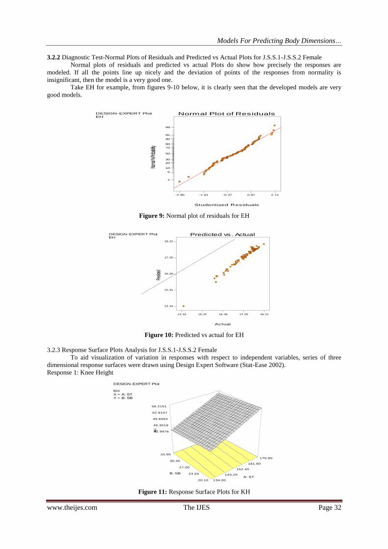
3.2.2 Diagnostic Test-Normal Plots of Residuals and Predicted vs Actual Plots for J.S.S.1-J.S.S.2 Female
Normal plots of residuals and predicted vs actual Plots do show how precisely the responses are
modeled. If all the points line up nicely and the deviation of points of the responses from normality is
insignificant, then the model is a very good one.
Take EH for example, from figures 9-10 below, it is clearly seen that the developed models are very
good models.
Figure 9: Normal plot of residuals for EH
Figure 10: Predicted vs actual for EH
3.2.3 Response Surface Plots Analysis for J.S.S.1-J.S.S.2 Female
To aid visualization of variation in responses with respect to independent variables, series of three
dimensional response surfaces were drawn using Design Expert Software (Stat-Ease 2002).
Response 1: Knee Height
Figure 11: Response Surface Plots for KH
DESIGN-EXPERT PlotEH
Studentized Residuals
Norma
l % Pr
obabili
ty
Normal Plot of Residuals
-2.85 -1.61 -0.37 0.87 2.11
1
5
10
20
30
50
70
80
90
95
99
DESIGN-EXPERT PlotEH
Actual
Predic
ted
Predicted vs. Actual
14.34
15.31
16.28
17.25
18.22
14.34 15.31 16.28 17.25 18.22
DESIGN-EXPERT Plot
KHX = A: STY = B: SB
42.9976
46.3019
49.6063
52.9107
56.2151
KH
134.00
143.20
152.40
161.60
170.80
20.10
23.55
27.00
30.45
33.90
A: ST
B: SB
Models For Predicting Body Dimensions…
www.theijes.com The IJES Page 33
Figure 11showed the interactive effect of ST and SB on the response (KH). At the low SB value of
20.10, KH decreases from 44.18 to 43.40, as ST increases from 134.00 to 137.00. Furthermore, KH increases
from 43.40 to 56.22, as ST increases from 137.00 to 170.80. This implied that KH decreases slightly as ST
increases and later increases as ST increases. The relationship is a linear one. Also, at high SB value of 33.9, KH
increases from 43.00 to 49.94, as ST increases from 134.00 to 155.30. Furthermore, KH increases from 49.94 to
55.03, as ST increases from 155.30 to 170.80. This implied that KH increases as ST increases in a linear
relationship.
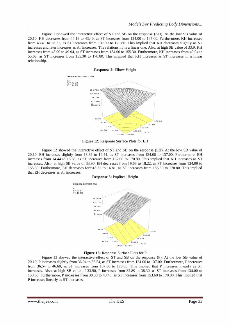
Response 2: Elbow Height
Figure 12: Response Surface Plots for EH
Figure 12 showed the interactive effect of ST and SB on the response (EH). At the low SB value of
20.10, EH increases slightly from 13.89 to 14.44, as ST increases from 134.00 to 137.00. Furthermore, EH
increases from 14.44 to 18.66, as ST increases from 137.00 to 170.80. This implied that KH increases as ST
increases. Also, at high SB value of 33.90, EH decreases from 19.68 to 18.22, as ST increases from 134.00 to
155.30. Furthermore, EH decreases form18.22 to 16.81, as ST increases from 155.30 to 170.80. This implied
that EH decreases as ST increases.
Response 3: Popliteal Height
Figure 13: Response Surface Plots for P
Figure 13 showed the interactive effect of ST and SB on the response (P). At the low SB value of
20.10, P increases slightly from 36.04 to 36.54, as ST increases from 134.00 to 137.00. Furthermore, P increases
from 36.54 to 46.60, as ST increases from 137.00 to 170.80. This implied that P increases linearly as ST
increases. Also, at high SB value of 33.90, P increases from 32.89 to 38.30, as ST increases from 134.00 to
153.60. Furthermore, P increases from 38.30 to 43.45, as ST increases from 153.60 to 170.80. This implied that
P increases linearly as ST increases.
DESIGN-EXPERT Plot
EHX = A: STY = B: SB
13.8913
15.3376
16.784
18.2303
19.6766
EH
134.00
143.20
152.40
161.60
170.80
20.10
23.55
27.00
30.45
33.90
A: ST
B: SB
DESIGN-EXPERT Plot
PX = A: STY = B: SB
32.8855
36.3141
39.7427
43.1713
46.5999
P
134.00
143.20
152.40
161.60
170.80
20.10
23.55
27.00
30.45
33.90
A: ST
B: SB
Models For Predicting Body Dimensions…
www.theijes.com The IJES Page 34
Response 4: Shoulder Height
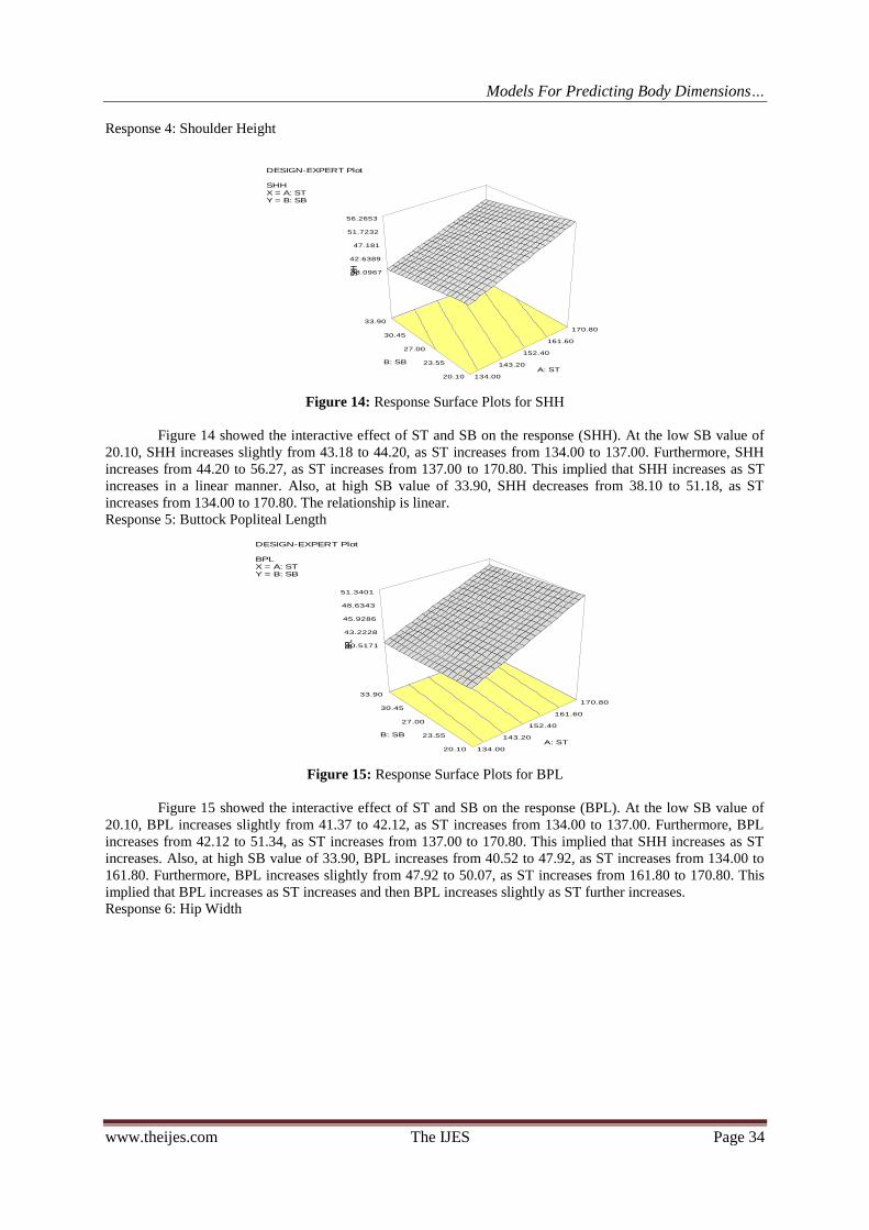
Figure 14: Response Surface Plots for SHH
Figure 14 showed the interactive effect of ST and SB on the response (SHH). At the low SB value of
20.10, SHH increases slightly from 43.18 to 44.20, as ST increases from 134.00 to 137.00. Furthermore, SHH
increases from 44.20 to 56.27, as ST increases from 137.00 to 170.80. This implied that SHH increases as ST
increases in a linear manner. Also, at high SB value of 33.90, SHH decreases from 38.10 to 51.18, as ST
increases from 134.00 to 170.80. The relationship is linear.
Response 5: Buttock Popliteal Length
Figure 15: Response Surface Plots for BPL
Figure 15 showed the interactive effect of ST and SB on the response (BPL). At the low SB value of
20.10, BPL increases slightly from 41.37 to 42.12, as ST increases from 134.00 to 137.00. Furthermore, BPL
increases from 42.12 to 51.34, as ST increases from 137.00 to 170.80. This implied that SHH increases as ST
increases. Also, at high SB value of 33.90, BPL increases from 40.52 to 47.92, as ST increases from 134.00 to
161.80. Furthermore, BPL increases slightly from 47.92 to 50.07, as ST increases from 161.80 to 170.80. This
implied that BPL increases as ST increases and then BPL increases slightly as ST further increases.
Response 6: Hip Width
DESIGN-EXPERT Plot
SHHX = A: STY = B: SB
38.0967
42.6389
47.181
51.7232
56.2653
SHH
134.00
143.20
152.40
161.60
170.80
20.10
23.55
27.00
30.45
33.90
A: ST
B: SB
DESIGN-EXPERT Plot
BPLX = A: STY = B: SB
40.5171
43.2228
45.9286
48.6343
51.3401
BPL
134.00
143.20
152.40
161.60
170.80
20.10
23.55
27.00
30.45
33.90
A: ST
B: SB

Models For Predicting Body Dimensions…
www.theijes.com The IJES Page 35
Figure 16: Response Surface Plots for HW
Figure 16 showed the interactive effect of ST and SB on the response (HW). At the low SB value of
20.10, HW increases slightly from 22.99 to 24.49, as ST increases from 134.00 to 137.00. Furthermore, HW
increases from 24.49 to 34.24, as ST increases from 137.00 to 170.80. This implied that HW increases as ST
increases. Also, at high SB value of 33.90, HW slightly decreases from 33.07 to 33.00 as ST increases from
132.80 to 170.80. This implied that HW decreases slightly as ST increases.
Table 8: Design Summary for J.S.S.1-J.S.S.2 Female
Study type: response surface Experiments: 231
Initial design: historical data Blocks: no blocks
Design model: quadratic
response name Units obs minimum Maximum trans Model
Y1 KH Cm 79 43.40 55.50 None Linear
Y2 EH Cm 79 14.44 18.22 None Quadratic
Y3 P Cm 79 34.77 44.77 None Linear
Y4 SHH Cm 79 41.26 53.29 None Linear
Y5 BPL Cm 79 40.96 50.41 None 2FI
Y6 HW Cm 79 23.88 32.08 None Quadratic
It is worthy of note that two independent variables sufficiently predicted the entire six responses in this
category of students (J.S.S.1-J.S.S.2 male and female). This may not be unconnected with the fact that students
in lower classes had small physique unlike their counterparts in middle and upper classes with well-built
physique.
Table 9: Summary of Co-efficient of Determination (R2) and Co-efficient of Variation (C.V.) of all the
Responses for J.S.S.1-J.S.S.2 Male/ J.S.S.1-J.S.S.2 Female.
Response R-Square Adj. R-Square Pred. R-Square C.V (%)
Male/Female Male/Female Male/Female Male/Female
KH 0.9117/0.9048 0.9059/0.9023 0.8871/0.8964 2.07/1.54
EH 0.9939/0.9789 0.9935/0.9774 0.9925/0.9719 0.34/0.54
P 0.8843/0.9077 0.8813/0.9053 0.8758/0.9024 2.40/1.57
SHH 0.9979/0.9983 0.9977/0.9982 0.9969/0.9981 0.32/0.21
BPL 0.9531/0.9986 0.9499/0.9986 0.9364/0.9984 1.40/0.16
HW 0.9932/0.9952 0.9928/0.9949 0.9874/0.9930 0.51/0.41
IV. DISCUSSIONS
4.1 Efficiencies of the Models. The most common performance measures for the efficiency of predictive models are co-efficient of determination
(R2) and co-efficient of variation (C.V) (Agha, et al., 2012). High value of R2 and low value of C.V are desirable. In this
study, twelve models were developed and the adjusted co-efficient of determination (R2) is greater than 0.85 in all.In general,
all the models showed good predictive ability (efficiency) as can be observed in Table 9. 75% of the models have adjusted
R2 value of over 90% and non-of the models have adjusted R2 value that is less than 85%. This confirmed the validity of the
models.Furthermore, according to Liyana-Pathirana and Shahidi (2005), a high coefficient of variation (CV) demonstrates
that variation in the mean value is large and does not sufficiently generate an acceptable response model. Therefore, CV <
10% has been suggested suitable in predicting the response surface models. From table 6, CV <= 2.40% for all the models.
This implied that the models exhibited very high predictive ability (they are efficient).
DESIGN-EXPERT Plot
HWX = A: STY = B: SB
22.8081
25.6671
28.526
31.385
34.2439
HW
134.00
143.20
152.40
161.60
170.80
20.10
23.55
27.00
30.45
33.90
A: ST
B: SB

Models For Predicting Body Dimensions…
www.theijes.com The IJES Page 36
4.2 Discussions of the Models. Using ergonomic principles, the common anthropometric measurements considered in the design of furniture are
popliteal height for seat height,buttock-popliteal length for seat depth, hip breadth for seat width, shoulder height for
backrest height, elbow height for table height, and knee height for underneath desk height. The current study developed 12
models considered necessary for the design of furniture for J.S.S.1-J.S.S.2 students. While the relationships among
standing height and length dimensions have usually been assumed linear, the present study confirmed that Out of the 12
models developed, 8 of them have non-linear relationships (representing 66.67%). Only 4 models (representing 33.33%)
have linear relationships.Moreover, the present study obtained a higher value of R2 which is 0.8813 and0.9953 compared
with R2_ 0.81 (r _ 0.90) obtained by Castellucciet al. (2010) and 0.844 obtained by Ismaila et al., (2014) for the model for
predicting popliteal height. Also, the value of R2 for EH in the present study is 0.9774 and 0.9935 which is far higher than
0.264 obtained by Agha et al., (2012) and 0.706 obtained by Ismaila et al., (2014). Indeed, Agha et al., (2012) reported that
EH cannot be predicted but rather measured. However, the present study showed otherwise. The performance of the models
developed in this study as compared with the previous ones is presented in table 10.
Table 10: Performance Comparism of the Developed Models with those of Previous Researches. Anthropometric dimensions R2 obtained in this study R2 obtained by Castellucci et al.,
(2012).
R2 obtained by Ismaila et
al., (2014). Min.-Max.
KH 0.9023-0.9059 0.921 0.725
EH 0.9774-0.9935 0.264 0.706
P 0.8813-0.9053 O.721 0.844
SHH 0.9977-0.9982 0.755 0.414
BPL 0.9499-0.9986 0.753 0.416
HW 0.9928-0.9949 Not applicable 0.199
According to Ismaila et al., (2014), it can be very expensive in developing countries to obtain anthropometric data
when needed, and as such, measuring one anthropometric value to determine others would be helpful and affordable.
Although economic reason is important but, at the same time, adequacy and effectiveness of the predictive models cannot be
compromised. The current study took these three factors (economic reason, adequacy and effectiveness) into consideration.
Using two anthropometric dimensions to predict six needed for the design of school furniture, as the case is for students in
J.S.S.1-J.S.S.2, is justifiable in view of the high predictive ability of the models.
V. CONCLUSION Ergonomic design of products and workplaces demands up-to-date anthropometric data which are not readily
available. In fact most practitioners do not know how the data for easily measured body dimensions can be used to estimate
body dimensions that are more difficult to measure. The present study, therefore, proposed 12 models that can be used to
estimate various anthropometric dimensions necessary for the design of furniture for use ofJ.S.S.1-J.S.S.2 students in
Ogbomoso, South Western Nigeria. The furniture industry would find in these models economical, adequate and effective
prediction tools.
REFERENCES [1] Adewole, N.A., Olorunnisola, A.O., (2010), “Characteristics of classroom chairs and desks in use in senior secondary schools in
Ibadan, Oyo State, Nigeria”, Journal of Emerging Trends in Engineering and Applied Sciences (JETEAS), Vol. 1 No. 2, pp 140-144. [2] Agha, S.R., Alnahhal, M.J., (2012), “Neural Network and multiple linear regressions to predict school children dimensions for
Ergonomic school furniture design”, Applied Ergonomics, Vol. 43, pp 979-984.
[3] Garcia – Acosta, G., Lange-Morales, K., (2007), “Definition of sizes for the design of school furniture for Bogota schools based on anthropometric criteria”, Ergonomics, Vol. 50 No. l0, pp 1626–1642.
[4] Ismaila, S.O., Akanbi, O.G., Ngassa, C.N. (2014), "Models for estimating the anthropometric dimensions using standing height for
furniture design", Journal of Engineering, Design and Technology, Vol. 12 No. 3, pp. 336-347. [5] Jeong, B.Y., Park,K.S. (1990), “Sex difference in Anthropometry for school furniture design”, Ergonomics, Vol. 33 No. 12, pp 1511-
1521.
[6] Liyana-Pathirana, C., Shahidi, F. (2005), “Optimization of extraction of phenolic compounds from wheat using response surface methodology”, Food Chem., Vol.93, pp 47-56.
[7] Molenbroek, J., Ramaekers, Y. (1996), “Anthropometric design of a size system for school furniture”, In: Robertson, S.A. (Ed.) 1996
Proceedings of the Annual Conference of the Ergonomics Society: Contemporary Ergonomics, 1996, Taylor and Francis, London, pp. 130–135.
[8] Niekerk, S., Louw, Q.A., Grimmer-Somers,K., Harvey, J. (2013), “The anthropometric match between high school learners of the caps
metropolitan area, Western cape, South Africa and their computer Workstation at school”, Applied Ergonomics, Vol. 44 No. 3, pp 366-371.
[9] Oyewole, S.A., Haight, J.M., Freivalds, A., (2010), “The ergonomic design of classroom furniture/computer work station for first
graders in the elementary school”, International Journal of Industrial Ergonomics, Vol. 40 No. 4, pp 437 – 447. [10] Parcells, C., Manfred,S., Hubbard, R.(1999), “Mismatch of classroom furniture and body dimensions, Empirical findings and health
implications”, Journal of Adolescent Health, Vol. 24 No. 4, pp 265-273.
[11] Reis, P., Moro, A.R., Da, S.J., Paschoarelli, L. Nunes, S.F., Peres, L. (2012), “Anthropometric aspects of body seated in school”. Work, Vol. 41, pp 907-914. DOI: 10.3233/WOR-2012-0262-907.
[12] Straker, L., Maslen, B., Burgress-Limerick, R., Johnson, P., Dennerlein, J. (2010), “Evidence-based guideline for wise use of
computers by children: physical development guidelines”, Ergonomics, Vol. 53 No. 4, pp458-477.
[13] Yeats, B. (1997), “Factors that may influence the postural health of schoolchildren (K-12)”, Work: A Journal of Prevention,
Assessment and Rehabilitation, Vol. 9, pp 45–55.
[14] You, H., Ryu, T. (2005), “Development of a hierarchical estimation method for anthropometric variables”, International Journal of Industrial Ergonomics, Vol. 35 No. 4, pp 331-343.