Modelling Volatility In Financial Time Series

i

Modelling Volatility In Financial Time

Series

By

Bruce Dralle Submitted in fulfillment of the academic

requirements for the degree of

Master of Science

in

Statistics

in the

School of Statistics and Actuarial Sciences

University of KwaZulu-Natal

Pietermaritzburg

2011

ii

Declaration

I, Bruce Dralle declare that

1. The research reported in this dissertation, except where otherwise indicated, is my

original research.

2. This dissertation has not been submitted for any degree or examination at any other

university.

3. This dissertation does not contain other persons’ data, pictures, graphs or other

information, unless specifically acknowledged as being sourced from other persons.

4. This dissertation does not contain other persons' writing, unless specifically

acknowledged as being sourced from other researchers. Where other written sources

have been quoted, then:

a. Their words have been re-written but the general information attributed to them

has been referenced

b. Where their exact words have been used, then their writing has been placed in

italics and inside quotation marks, and referenced.

5. This dissertation does not contain text, graphics or tables copied and pasted from the

Internet, unless specifically acknowledged, and the source being detailed in the

disseration and in the References sections.

…………………………….. .................................. Bruce Dralle Date .............................. ................................. Dr. Shaun Ramroop Date

iii

Acknowledgments

I would like to thank my supervisors, Doctor Shaun Ramroop and Professor Henry Mwambi, for all

their help while working on this dissertation. This work would not have been possible without

their valuable input and advice. Thank you to my friends and family for all the support and

encouragement. I would also like to say thank you to Brenda for your hard work helping me to

correct my English.

iv

Abstract

The objective of this dissertation is to model the volatility of financial time series data using ARCH,

GARCH and stochastic volatility models. It is found that the ARCH and GARCH models are easy to

fit compared to the stochastic volatility models which present problems with respect to the

distributional assumptions that need to be made. For this reason the ARCH and GARCH models

remain more widely used than the stochastic volatility models. The ARCH, GARCH and stochastic

volatility models are fitted to four data sets consisting of daily closing prices of gold mining

companies listed on the Johannesburg stock exchange. The companies are Anglo Gold Ashanti Ltd,

DRD Gold Ltd, Gold Fields Ltd and Harmony Gold Mining Company Ltd. The best fitting ARCH and

GARCH models are identified along with the best error distribution and then diagnostics are

performed to ensure adequacy of the models. It was found throughout that the student-t

distribution was the best error distribution to use for each data set. The results from the stochastic

volatility models were in agreement with those obtained from the ARCH and GARCH models. The

stochastic volatility models are, however, restricted to the form of an AR(1) process due to the

complexities involved in fitting higher order models.

v

Contents

Chapter One ........................................................................................................................................ 1

1 Introduction.................................................................................................................................. 1

Chapter Two ........................................................................................................................................ 4

2 Data Description and Exploration ................................................................................................ 4

2.1 Data Description ........................................................................................................................ 4

2.2 Data Exploration ........................................................................................................................ 4

2.2.1 Anglo Gold Ashanti Ltd ....................................................................................................... 4

2.2.2 DRD Gold Ltd ...................................................................................................................... 8

2.2.3 Gold Fields Ltd .................................................................................................................. 12

2.2.4 Harmony Gold Mining Company Ltd ................................................................................ 16

Chapter Three ................................................................................................................................... 21

3 ARCH and GARCH Models .......................................................................................................... 21

3.1 The ARCH Model ..................................................................................................................... 21

3.1.1 The ARCH(1) Model .......................................................................................................... 21

3.1.2 The ARCH(q) Model .......................................................................................................... 29

3.2 The GARCH Model ................................................................................................................... 31

3.2.1 The GARCH(1,1) Model .................................................................................................... 32

3.2.2 The GARCH(p,q) Model .................................................................................................... 41

3.3 Extensions of the GARCH Model ............................................................................................. 45

3.4 Testing for ARCH ..................................................................................................................... 48

3.5 Model Selection Criteria .......................................................................................................... 49

3.6 Model Diagnostics ................................................................................................................... 50

3.7 Multivariate ARCH and GARCH Models .................................................................................. 50

3.7.1 Multivariate ARCH ............................................................................................................ 51

3.7.2 Multivariate GARCH ......................................................................................................... 52

Chapter Four ..................................................................................................................................... 54

4 Application of ARCH and GARCH Models ................................................................................... 54

4.1 Introduction ......................................................................................................................... 54

4.2 Selecting the Best Model .................................................................................................... 54

vi

4.3 Fitting the Model ................................................................................................................. 54

4.4 Analysis of the Anglo Gold Ashanti Ltd Data ....................................................................... 55

4.5 Analysis of the DRD Gold Ltd Data ...................................................................................... 64

4.6 Analysis of the Gold Fields Ltd Data .................................................................................... 70

4.7 Analysis of the Harmony Gold Mining Company Ltd Data .................................................. 75

Chapter Five ...................................................................................................................................... 81

5 Stochastic Volatility Models ....................................................................................................... 81

5.1 The Stochastic Volatility Model ........................................................................................... 81

5.2 State-Space Models ............................................................................................................. 82

5.3 The Kalman Filter................................................................................................................. 83

5.4 The Kalman Smoother ......................................................................................................... 86

5.5 The Lag One Covariance Smoother ..................................................................................... 87

5.6 Maximum Likelihood Estimation ......................................................................................... 89

5.7 The Expectation Maximization Algorithm ........................................................................... 91

5.8 The Stochastic Volatility Model ........................................................................................... 94

Chapter Six ........................................................................................................................................ 97

6 Application of Stochastic Volatility Models ................................................................................ 97

6.1 Introduction ......................................................................................................................... 97

6.2 Stochastic Volatility Model for the Anglo Gold Ashanti Ltd Data ...................................... 97

6.3 Stochastic Volatility Model for the DRD Gold Ltd Data ....................................................... 98

6.4 Stochastic Volatility Model for the Gold Fields Ltd Data .................................................... 99

6.5 Stochastic Volatility Model for the Harmony Gold Mining Company Ltd Data .................. 99

Chapter Seven ................................................................................................................................. 101

7 Conclusion ................................................................................................................................ 101

Appendix A ...................................................................................................................................... 105

Theorem 1 ................................................................................................................................... 105

Result 1 ........................................................................................................................................ 105

Appendix B ...................................................................................................................................... 107

SAS Code for ARCH and GARCH Models ..................................................................................... 107

Anglo Gold Ashanti GARCH(1,2) Model .................................................................................. 107

vii

DRD Gold GARCH(3,3) Model .................................................................................................. 107

Gold Fields GARCH(1,2) Model ................................................................................................ 108

Harmony Gold Mining Company GARCH(2,1) Model ............................................................. 108

R Code for the Stochastic Volatility Models ................................................................................ 109

Bibliography .................................................................................................................................... 113

viii

List of Tables

Table 1: Anglo Gold Ashanti Preliminary Results ................................................................................ 5

Table 2: Anglo Gold Ashanti Tests for Normality ................................................................................ 5

Table 3: DRD Gold Preliminary Results ............................................................................................... 9

Table 4: DRD Gold Tests for Normality ............................................................................................... 9

Table 5: Gold Fields Preliminary Results ........................................................................................... 13

Table 6: Gold Fields Tests for Normality ........................................................................................... 13

Table 7: Harmony Gold Mining Company Preliminary Results ......................................................... 17

Table 8: Harmony Gold Mining Company Tests for Normality ......................................................... 17

Table 9: Anglo Gold Ashanti Q and LM Tests for ARCH Disturbances ............................................... 55

Table 10: Anglo Gold Ashanti best models based on the three selection criteria ............................ 56

Table 11: Fit Statistics for the ARCH(2) Model .................................................................................. 57

Table 12: Parameter Estimates with Standard Errors and p-values for the ARCH(2) Model ............ 58

Table 13: Fit Statistics for the GARCH(1,1) Model ............................................................................ 59

Table 14: Parameter Estimates with Standard Errors and p-values for the GARCH(1,1) Model ...... 59



Table 17: Fit Statistics for the IGARCH(1,2) Model ........................................................................... 62

Table 18: Anglo Gold Ashanti Testing for ARCH Disturbances after fitting the GARCH(1,2) Model . 63

Table 19: DRD Gold Q and LM Tests for ARCH Disturbances ............................................................ 64

Table 20: DRD Gold best models based on the three selection criteria ........................................... 65

Table 21: Fit Statistics for the GARCH(3,3) ........................................................................................ 66


Table 23: Fit Statistics for the ARCH(3) Model .................................................................................. 67

Table 24: Parameter Estimates with Standard Errors and p-values for the ARCH(3) Model ............ 67

Table 25: DRD Gold Testing for ARCH Disturbances after fitting the GARCH(3,3) Model ................ 69

Table 26: Gold Fields Q and LM Tests for ARCH Disturbances .......................................................... 70

Table 27: Gold Fields best models based on the three selection criteria ......................................... 71



ix

Table 30: Fit Statistics for the IGARCH(1,2) Model ........................................................................... 73

Table 31: Gold Fields Testing for ARCH Disturbances after fitting the GARCH(1,2) Model .............. 74

Table 32: Harmony Gold Mining Company Q and LM Tests for ARCH Disturbances ........................ 75

Table 33: Harmony Gold Mining Company best models based on the three selection criteria ....... 76





Table 38: Harmony Gold Mining Company Testing for ARCH Disturbances after fitting the

GARCH(2,1) Model ............................................................................................................................ 80

Table 39: Parameter Estimates for the Anglo Gold Ashanti Stochastic Volatility Model ................. 98

Table 40: Parameter Estimates for the DRD Gold Stochastic Volatility Model ................................. 98

Table 41: Parameter Estimates for the Gold Fields Stochastic Volatility Model .............................. 99

Table 42: Parameter Estimates for the Harmony Gold Stochastic Volatility Model ....................... 100

x

List of Figures

Figure 1: Anglo Gold Ashanti Daily Closing Price ................................................................................ 6

Figure 2: Histogram of the Daily Return for Anglo Gold Ashanti ........................................................ 6

Figure 3: Anglo Gold Ashanti Daily Return .......................................................................................... 7

Figure 4: Anglo Gold Ashanti Daily Squared Return ............................................................................ 7

Figure 5: ACF and PACF for Anglo Gold Ashanti Daily Return ............................................................. 8

Figure 6: ACF and PACF for Anglo Gold Ashanti Daily Squared Return ............................................... 8

Figure 7: DRD Gold Daily Closing Price .............................................................................................. 10

Figure 8: Histogram of the Daily Return for DRD Gold ..................................................................... 10

Figure 9: DRD Gold Daily Return ....................................................................................................... 11

Figure 10: DRD Gold Daily Squared Return ....................................................................................... 11

Figure 11: ACF and PACF for DRD Gold Daily Return ........................................................................ 12

Figure 12: ACF and PACF for DRD Gold Daily Squared Return .......................................................... 12

Figure 13: Gold Fields Daily Closing Price.......................................................................................... 14

Figure 14: Histogram of Daily Return for Gold Fields ........................................................................ 14

Figure 15: Gold Fields Daily Return ................................................................................................... 15

Figure 16: Gold Fields Daily Squared Return ..................................................................................... 15

Figure 17: ACF and PACF for Gold Fields Daily Return ...................................................................... 16

Figure 18: ACF and PACF for Gold Fields Daily Squared Return ........................................................ 16

Figure 19: Harmony Gold Mining Company Daily Closing Price ....................................................... 18

Figure 20: Histogram of Daily Return for Harmony Gold Mining Company ..................................... 18

Figure 21: Harmony Gold Mining Company Daily Return ................................................................. 19

Figure 22: Harmony Gold Mining Company Daily Squared Return ................................................... 19

Figure 23: ACF and PACF for Harmony Gold Mining Company Daily Return .................................... 20

Figure 24: ACF and PACF for Harmony Gold Mining Company Daily Squared Return ...................... 20

Figure 25: ACF and PACF of Squared Residuals for the Anglo Gold Ashanti AR(8) Model ................ 56

Figure 26: ACF and PACF of Residuals for the GARCH(1,2) Model .................................................... 62

Figure 27: ACF and PACF of Squared Residuals for the GARCH(1,2) Model ..................................... 63

Figure 28: ACF and PACF of Squared Residuals for the DRD Gold AR(1) Model ............................... 65


xi


Figure 31: ACF and PACF of Squared Residuals for the Gold Fields AR(8) Model ............................. 71



Figure 34: ACF and PACF of Squared Residuals for the Harmony Gold Mining Company AR(2) Model

........................................................................................................................................................... 76



1

Chapter One

1 Introduction

Modeling financial time series focuses on the valuation of an asset over time. This is often a

complex and difficult problem due to the number of different series available, including stock

prices, exchange rate data, and interest rates, just to name a few. A further complication is that

the series can often be viewed using different frequencies of observation; this may be every

second, every minute, every hour, every day and so on (Francq & Zakoian, 2010, p. 7). One of the

distinguishing features of financial time series is that they bring about an element of risk or

uncertainty (Tsay, 2005, p. 1). This risk or uncertainty can be crudely measured by the volatility of

an asset. A major problem that is often encountered when modeling financial time series is the

concept of nonstationarity. Nonstationarity occurs when the underlying rules that generate the

time series change on occasion, often without any prior indication that a change is about to

happen. This complicates the modeling process as the traditional autoregressive moving average

(ARMA) models are based on the assumption of stationarity and, therefore, may be unreliable.

Reliable and complementary models are the Autoregressive Conditional Heteroscedastic (ARCH),

Generalized Autoregressive Conditional Heteroscedastic (GARCH) and Stochastic Volatility models.

When dealing with a nonstationary financial time series you are essentially dealing with a high

level of uncertainty and, therefore, maximum risk to your investment (Sherry & Sherry, 2000, p. 6).

The purpose of this study will be the modeling of the volatility of an asset over time. This will be

done using stock price time series data with a daily observation frequency. If we use a model that

depends on constant variance when the series is in actual fact non-constant, then one of the

possible implications would be that our standard error estimates could be incorrect (Brooks, 2008,

p. 386). Therefore, we require models that involve conditional heteroscedasticity.

Heteroscedasticity refers to non-constant variance. The models that involve conditional

heteroscedasticity, that will be used for this study, are the Autoregressive Conditional

Heteroscedastic (ARCH) models which were first introduced by Engle (1982); the Generalized

Autoregressive Conditional Heteroscedastic (GARCH) models, which generalize the ARCH models

of Engle (1982), and were first introduced by Bollerslev (1986); and Stochastic Volatility models

2

(Kim, Shephard, & Chib, 1998). The ARCH family of models are observation driven models,

whereas the Stochastic Volatility models are parameter driven models. Some of the motivations,

apart from the presence of heteroscedasticity, for the use of the ARCH family of models is that

time series of financial asset returns often exhibit volatility clustering and fat tails or leptokurtosis.

Volatility clustering occurs when large changes in an asset's price are typically followed by more

large changes of either sign (positive or negative) and small changes in the price are typically

followed by more small changes again of either sign (positive or negative). This implies that the

current volatility is strongly related to the volatility present in the immediate past (Brooks, 2008,

pp. 386-387; Francq & Zakoian, 2010, p. 9). Leptokurtosis occurs when the distribution of the

return of an asset exhibits fatter tails and is more peaked at zero than that of a standard Gaussian

distribution. Another reason for the use of the ARCH family of models is that financial time series

often exhibit a leverage effect, which is an asymmetry of the impact that the past positive and

negative values have on the current volatility. It is often seen that negative returns (a price

decrease) tend to increase the volatility by a larger amount than a positive return (price increase)

of the same amount (Francq & Zakoian, 2010, pp. 9-10). The ARCH family of models have proved

useful in accounting for the heteroscedasticity, volatility clustering, and leptokurtosis which are

often present in financial time series.

As already stated the alternative to the ARCH family of models, which are observation driven

models, are the parameter driven models where the variance is modeled as an unobserved

component that follows some underlying latent stochastic process. These models are referred to

as Stochastic Volatility (SV) models. It should be noted that it is not the case that the GARCH family

of models are a type of Stochastic Volatility model. They differ in that the GARCH models are

completely deterministic and use all the information that is available up to that of the previous

period. This means that there is no error term in the variance equation of the GARCH model, the

error term appears only in the mean equation. The Stochastic Volatility model includes a second

error term, this error term enters into the conditional variance equation (Brooks, 2008, p. 427).

The Stochastic Volatility models have not been as widely used as the ARCH family of models. One

of the reasons for this is that the likelihood for the Stochastic Volatility models is not easy to

evaluate, which is not the case with the ARCH models (Shimada & Tsukuda, 2005, p. 3). There are

two reasons for the difficulty in estimating the likelihood for Stochastic Volatility models. Firstly,

3

because the variance is modeled as an unobserved component and, secondly the model is non-

Gaussian. This results in the likelihood being complicated and difficult to work with. Another

disadvantage of using Stochastic volatility models is that the estimation process consists of two

stages: parameter estimation and estimation of the latent volatility. Methods that work well for

the parameter estimation may perform poorly when estimating the latent volatility (Mahieu &

Schotman, 1998, pp. 333-334).

The study of volatility has applications in many areas of finance: it plays an important role in

managing risk and aids in the implementation of economic policy by government and private

institutions. Proper risk management and a well implemented economic policy allow for the

maximization of profits for both financial institutions and the individual investor. This leads to a

strengthened economy that can play a significant role in global markets.

4

Chapter Two

2 Data Description and Exploration

2.1 Data Description

Four data sets will be used to investigate the use of ARCH, GARCH and Stochastic Volatility models.

The data sets that have been selected for use are for gold mining companies listed on the

Johannesburg Stock Exchange. The companies selected are Anglo Gold Ashanti Ltd, DRD Gold Ltd,

Gold Fields Ltd and Harmony Gold Mining Company Ltd. The data sets consist of the daily closing

price for each company.

Many financial studies model the return instead of the price, as the return series is often easier to

handle than the original price series and the return also provides a summary that is free of scale

(Tsay, 2005, p. 2). The daily closing price is used to calculate the daily return which is given by

(2.1)

where and are the closing prices at times and , respectively. This is known as the

simple return (Tsay, 2005, p. 3). It is also common to use log returns for analysis. The log return is

given by

(2.2)

(Ruppert, 2004, p. 76). While performing the exploratory analysis for the four data sets, it was

found that the log return had a distribution that was closer to normality than the distribution for

the simple return. For this reason, the log return will be used for the data analysis; the log return

will simply be referred to as the return.

2.2 Data Exploration

2.2.1 Anglo Gold Ashanti Ltd

The data available for AngloGold Ashanti consists of a time series of daily closing prices with 4188

observations from 3 January 1994 to 22 January 2010. A plot of the closing price is presented in

5

Figure 1, where it can be seen that the closing price series shows periods of large price movements

and periods of small price movements. This would suggest that there is some volatility clustering

in the series. The return series consists of 4187 observations because one observation is lost when

calculating the return. Figure 3 shows the plot of daily returns for the series and Figure 4 shows a

plot of the squared returns. From the plots of the returns and squared returns, evidence of

volatility clustering can be seen. Some preliminary results for the return series are given in Table 1.

The results show that the return series has a high kurtosis which suggests that the series is not

normally distributed. This is confirmed by the tests for normality which are given in Table 2 and

from a visual inspection of the histogram of the return shown in Figure 2.

Table 1: Anglo Gold Ashanti Preliminary Results

Anglo Gold Ashanti Preliminary Results

Log Return Squared Log Return

Mean 0.00007 0.0007

Median 0.0000 0.0002

Maximum 0.1756 0.0309

Minimum -0.1233 0.0000

Standard Deviation 0.0260 0.0015

Skewness 0.3977 6.6147

Kurtosis 2.8577 74.7490

Table 2: Anglo Gold Ashanti Tests for Normality

Anglo Gold Ashanti Tests for Normality


Test Statistic p-value Statistic p-value

Kolmogorov-Smirnov 0.0602 <0.010 0.3250 <0.010

Cramer-von Mises 5.9008 <0.005 129.7418 <0.005

Anderson-Darling 32.4484 <0.005 656.0393 <0.005

6

Figure 1: Anglo Gold Ashanti Daily Closing Price

Figure 2: Histogram of the Daily Return for Anglo Gold Ashanti

0

5000

10000

15000

20000

25000

30000

35000

40000

03

-Jan

-94

03

-Jan

-95

03

-Jan

-96

03

-Jan

-97

03

-Jan

-98

03

-Jan

-99

03

-Jan

-00

03

-Jan

-01

03

-Jan

-02

03

-Jan

-03

03

-Jan

-04

03

-Jan

-05

03

-Jan

-06

03

-Jan

-07

03

-Jan

-08

03

-Jan

-09

03

-Jan

-10

Clo

sin

g P

rice

(c)

Date

Anglo Gold Daily Closing Price

7

Figure 3: Anglo Gold Ashanti Daily Return

Figure 4: Anglo Gold Ashanti Daily Squared Return

The autocorrelation (ACF) and partial autocorrelation functions (PACF) for the daily return are

given in Figure 5. The ACF shows that there is some minor serial correlation at lags 1 and 8 while

the PACF has significant spikes at lags 1 and 8.

-0.1500

-0.1000

-0.0500

0.0000

0.0500

0.1000

0.1500

0.2000

0.2500

04

-Jan

-94

04

-Jan

-95

04

-Jan

-96

04

-Jan

-97

04

-Jan

-98

04

-Jan

-99

04

-Jan

-00

04

-Jan

-01

04

-Jan

-02

04

-Jan

-03

04

-Jan

-04

04

-Jan

-05

04

-Jan

-06

04

-Jan

-07

04

-Jan

-08

04

-Jan

-09

04

-Jan

-10

Re

turn

Date

Anglo Gold Daily Return

0.0000

0.0050

0.0100

0.0150

0.0200

0.0250

0.0300

0.0350

0.0400

04

-Jan

-94

04

-Jan

-95

04

-Jan

-96

04

-Jan

-97

04

-Jan

-98

04

-Jan

-99

04

-Jan

-00

04

-Jan

-01

04

-Jan

-02

04

-Jan

-03

04

-Jan

-04

04

-Jan

-05

04

-Jan

-06

04

-Jan

-07

04

-Jan

-08

04

-Jan

-09

04

-Jan

-10

Squ

are

d R

etu

rn

Date

Anglo Gold Daily Squared Return

8

Figure 5: ACF and PACF for Anglo Gold Ashanti Daily Return

Figure 6: ACF and PACF for Anglo Gold Ashanti Daily Squared Return

The autocorrelation (ACF) and partial autocorrelation functions (PACF) for the daily squared return

are given in Figure 6. The ACF and PACF both show significant spikes which indicates the presence

of an ARCH effect.

2.2.2 DRD Gold Ltd

The data available for DRD Gold consists of a time series of daily closing prices with 4186

observations from 3 January 1994 to 22 January 2010. A plot of the daily closing price is presented

in Figure 7. The plot reveals periods of large price movements, as well as periods of small price

movements. This indicates that there may be some volatility clustering in the series. The return

series consists of 4185 observations because one observation is lost when calculating the return.

Figure 9 shows a plot of daily returns and Figure 10 shows a plot of the squared daily returns. The

plots of returns and squared returns show evidence of volatility clustering. Preliminary results for

the return can be found in Table 3 where it is seen that the return has a high kurtosis, along with

9

some negative skewness, which suggests that the return series is not normally distributed. This is

confirmed by the test for normality, as shown in Table 4, and from a visual inspection of the

histogram of the return, shown in Figure 8.

Table 3: DRD Gold Preliminary Results

DRD Gold Preliminary Results


Mean -0.0006 0.0017

Median 0.0000 0.0003

Maximum 0.3316 0.2508

Minimim -0.5008 0.0000


Skewness -0.1823 20.5158

Kurtosis 10.9998 686.7178

Table 4: DRD Gold Tests for Normality

DRD Gold Tests for Normality




Cramer-von Mises 18.5252 <0.005 184.6000 <0.005


10

Figure 7: DRD Gold Daily Closing Price

Figure 8: Histogram of the Daily Return for DRD Gold

0

1000

2000

3000

4000

5000

6000

7000

03

-Jan

-94

03

-Jan

-95

03

-Jan

-96

03

-Jan

-97

03

-Jan

-98

03

-Jan

-99

03

-Jan

-00

03

-Jan

-01

03

-Jan

-02

03

-Jan

-03

03

-Jan

-04

03

-Jan

-05

03

-Jan

-06

03

-Jan

-07

03

-Jan

-08

03

-Jan

-09

03

-Jan

-10

Clo

sin

g P

rice

(c)

Date

DRD Gold Daily Closing Price

11

Figure 9: DRD Gold Daily Return

Figure 10: DRD Gold Daily Squared Return

The autocorrelation (ACF) and partial autocorrelation functions (PACF) for the daily return can be

seen in Figure 11. The ACF shows some minor serial correlation at lags 1 and 17, with the PACF

showing significant spikes at the same lags.

-0.5 -0.4 -0.3 -0.2 -0.1

0 0.1 0.2 0.3 0.4 0.5

04

-Jan

-94

04

-Jan

-95

04

-Jan

-96

04

-Jan

-97

04

-Jan

-98

04

-Jan

-99

04

-Jan

-00

04

-Jan

-01

04

-Jan

-02

04

-Jan

-03

04

-Jan

-04

04

-Jan

-05

04

-Jan

-06

04

-Jan

-07

04

-Jan

-08

04

-Jan

-09

04

-Jan

-10

Re

turn

Date

DRD Gold Daily Return

0 0.02 0.04 0.06 0.08

0.1 0.12 0.14 0.16 0.18

04

-Jan

-94

04

-Jan

-95

04

-Jan

-96

04

-Jan

-97

04

-Jan

-98

04

-Jan

-99

04

-Jan

-00

04

-Jan

-01

04

-Jan

-02

04

-Jan

-03

04

-Jan

-04

04

-Jan

-05

04

-Jan

-06

04

-Jan

-07

04

-Jan

-08

04

-Jan

-09

04

-Jan

-10

Squ

are

d R

etu

rn

Date

DRD Gold Daily Squared Return

12

Figure 11: ACF and PACF for DRD Gold Daily Return

Figure 12: ACF and PACF for DRD Gold Daily Squared Return


are given Figure 12. The ACF shows some minor serial correlation at lags 2, 3, and 4 with the PACF

showing some minor serial correlation at lags 1, 2, and 3. This indicates the presence of an ARCH

effect.

2.2.3 Gold Fields Ltd

The data available for Gold Fields Ltd consists of a time series of daily closing prices with 3123

observations from 2 February 1998 to 22 January 2010. A plot of the closing prices is presented in

Figure 13. The plot shows some periods of low volatility and other periods of high volatility. The

return series consists of 3122 observations because one observation is lost when calculating the

return. Figure 15 shows a plot of the daily return series and Figure 16 shows a plot of the squared

return series. The plots of the return series and the squared return series show some evidence of

volatility clustering. Preliminary results for the return and squared return series can be found in

13

Table 5 where it is seen that the return series has a high kurtosis and some negative skewness

suggesting that the series is not normally distributed. This is confirmed by the tests for normality

which can be seen in Table 6 and from a visual inspection of the histograms of the return shown in

Figure 14.

Table 5: Gold Fields Preliminary Results

Gold Fields Preliminary Results


Mean 0.0003 0.0012

Median 0.0000 0.0003

Maximum 0.2490 0.1885

Minimum -0.4342 0.0000


Skewness -0.1446 28.1367

Kurtosis 11.6058 1141.722

Table 6: Gold Fields Tests for Normality

Gold Fields Tests for Normality


Test Statistic p-value Statistics p-value


Cramer-von Mises 6.0041 <0.005 135.204 <0.005


14

Figure 13: Gold Fields Daily Closing Price

Figure 14: Histogram of Daily Return for Gold Fields

0 2000 4000 6000 8000

10000 12000 14000 16000 18000 20000

02

-Feb

-98

02

-Feb

-99

02

-Feb

-00

02

-Feb

-01

02

-Feb

-02

02

-Feb

-03

02

-Feb

-04

02

-Feb

-05

02

-Feb

-06

02

-Feb

-07

02

-Feb

-08

02

-Feb

-09

Clo

sin

g P

rice

(c)

Date

Gold Fields Daily Closing Price

15

Figure 15: Gold Fields Daily Return

Figure 16: Gold Fields Daily Squared Return


seen in Figure 17. The ACF shows some minor serial correlations at lags 1, 4, 7, and 23, while the

PACF has significant spikes at the same lags.

-0.4

-0.3

-0.2

-0.1

0

0.1

0.2

0.3

0.4

03

-Feb

-98

03

-Feb

-99

03

-Feb

-00

03

-Feb

-01

03

-Feb

-02

03

-Feb

-03

03

-Feb

-04

03

-Feb

-05

03

-Feb

-06

03

-Feb

-07

03

-Feb

-08

03

-Feb

-09

Re

turn

Date

Gold Fields Daily Return

0

0.02

0.04

0.06

0.08

0.1

0.12

0.14

03

-Feb

-98

03

-Feb

-99

03

-Feb

-00

03

-Feb

-01

03

-Feb

-02

03

-Feb

-03

03

-Feb

-04

03

-Feb

-05

03

-Feb

-06

03

-Feb

-07

03

-Feb

-08

03

-Feb

-09

Squ

are

d R

etu

rn

Date

Gold Fields Daily Squared Return

16

Figure 17: ACF and PACF for Gold Fields Daily Return

Figure 18: ACF and PACF for Gold Fields Daily Squared Return


are given Figure 18. The ACF shows some minor serial correlation at lags 2, 4, and 5 with the PACF

showing some minor serial correlation at lags 1, 3, and 5. This indicates the presence of an ARCH

effect.

2.2.4 Harmony Gold Mining Company Ltd

The data available for Harmony Gold Mining Company consists of a time series of closing prices

with 4188 observations from 3 January 1994 to 22 January 2010. A plot of the closing price is

presented in Figure 19. The first half of the series exhibits relatively low volatility whilst the second

half of the series shows an increase in the volatility. The return series consists of 4187

observations because one observation is lost when calculating the return. Figure 21 shows the plot

of daily returns for the series and Figure 22 shows a plot of squared returns. The plot of returns

and squared returns shows some evidence of volatility clustering in the series. Preliminary results

17

for the return and squared return series are given in Table 7, where it can be seen that there is a

high kurtosis and some positive skewness for the return series, which suggests that the series is

not normally distributed. This is confirmed by the tests for normality, where p-values are found to

be less than 0.05, which can be found in Table 8 and from a visual inspection of the histogram of

the return series shown in Figure 20.

Table 7: Harmony Gold Mining Company Preliminary Results

Harmony Gold Mining Company Preliminary Results


Mean 0.00028 0.0010

Median 0.0000 0.0002

Maximum 0.2287 5.2296

Minimum -0.1728 0.0000


Skewness 0.2912 7.5668

Kurtosis 3.9907 90.9873

Table 8: Harmony Gold Mining Company Tests for Normality

Harmony Gold Mining Company Tests for Normality




Cramer-von Mises 11.1683 <0.005 142.4249 <0.005


18

Figure 19: Harmony Gold Mining Company Daily Closing Price

Figure 20: Histogram of Daily Return for Harmony Gold Mining Company

0 2000 4000 6000 8000

10000 12000 14000 16000 18000 20000

03

-Jan

-94

03

-Jan

-95

03

-Jan

-96

03

-Jan

-97

03

-Jan

-98

03

-Jan

-99

03

-Jan

-00

03

-Jan

-01

03

-Jan

-02

03

-Jan

-03

03

-Jan

-04

03

-Jan

-05

03

-Jan

-06

03

-Jan

-07

03

-Jan

-08

03

-Jan

-09

03

-Jan

-10

Clo

sin

g P

rice

(c)

Date

Harmony Gold Mining Company Daily Closing Price

19

Figure 21: Harmony Gold Mining Company Daily Return

Figure 22: Harmony Gold Mining Company Daily Squared Return


seen in Figure 23. The ACF shows some minor serial correlation at lag 1, while the PACF shows

significant spikes at lags 1 and 15.

-0.2 -0.15

-0.1 -0.05

0 0.05

0.1 0.15

0.2 0.25

0.3

04

-Jan

-94

04

-Jan

-95

04

-Jan

-96

04

-Jan

-97

04

-Jan

-98

04

-Jan

-99

04

-Jan

-00

04

-Jan

-01

04

-Jan

-02

04

-Jan

-03

04

-Jan

-04

04

-Jan

-05

04

-Jan

-06

04

-Jan

-07

04

-Jan

-08

04

-Jan

-09

04

-Jan

-10

Re

turn

Date

Harmony Gold Mining Company Daily Return

0

0.01

0.02

0.03

0.04

0.05

0.06

0.07

04

-Jan

-94

04

-Jan

-95

04

-Jan

-96

04

-Jan

-97

04

-Jan

-98

04

-Jan

-99

04

-Jan

-00

04

-Jan

-01

04

-Jan

-02

04

-Jan

-03

04

-Jan

-04

04

-Jan

-05

04

-Jan

-06

04

-Jan

-07

04

-Jan

-08

04

-Jan

-09

04

-Jan

-10

Squ

are

d R

etu

rn

Date

Harmony Gold Mining Company Daily Squared Return

20

Figure 23: ACF and PACF for Harmony Gold Mining Company Daily Return

Figure 24: ACF and PACF for Harmony Gold Mining Company Daily Squared Return


are given Figure 24. The ACF shows many significant spikes with the PACF showing some minor

serial correlation at lags 1, 2, 3, 4, 5, 6 and 7. This indicates the presence of an ARCH effect.

21

Chapter Three

3 ARCH and GARCH Models

Until recently the main focus of economic time series modeling was based on the conditional first

moments. Any dependency on higher moments was treated as nuisance (Bollerslev, Engle, &

Nelson, ARCH Models, 1994, p. 2961). When making use of ARMA models there is an assumption

of stationarity. This implies that we are making the assumption that the time series exhibits a

constant variance, that is that the variance remains constant over time. This assumption is,

however, an unrealistic one because many financial time series are often covariance

nonstationary. There has been an increased focus on the importance of modeling risk and this has

led to the development of models to allow for time varying variances and covariances (Bollerslev,

Engle, & Nelson, ARCH Models, 1994, p. 2961). A class of models that allow for the presence of

time varying variances and covariances are the ARCH family of models which were first introduced

by Engle (1982). The ARCH models were later extended by Bollerslev (1986) to a more general

form, known as GARCH models. ARCH and GARCH models, which are the focus of this chapter,

have been widely used to analyze data on exchange rates and stock prices (Berkes, Horvath, &

Kokoszka, 2003, p. 201) and play an increasingly important role in the management of risk

scenario.

3.1 The ARCH Model

The autoregressive conditional heteroscedastic (ARCH) model was first introduced by Engle (1982)

to model changes in volatility (Shumway & Stoffer, 2006, p. 280). The ARCH model allows for the

conditional error variance present in an ARMA process to depend on the past squared errors (Box,

Jenkins, & Reinsel, 2008, p. 414). This is different from the ARMA process, in which errors are

assumed to be independent. In order to understand the ARCH model it is useful to first look at the

ARCH(1) model and some of the properties associated with it.

3.1.1 The ARCH(1) Model

Let be the return of an asset at time . The return series should be serially uncorrelated or

only have some minor serial correlations at lower orders when the interest is on the study of

volatility. The series should however be dependent. The conditional mean and variance of given

are

22

and

where is the information set or history at time . Now let

where is the in the form of an ARMA model with some explanatory variables given by

(Tsay, 2005, pp. 99-100).

More explanation on ARMA and related models can be found in (Tsay, 2005) and (Box, Jenkins, &

Reinsel, 2008).

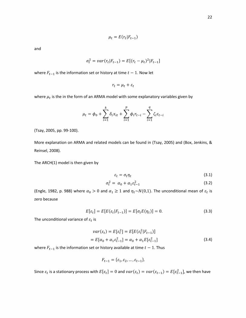
The ARCH(1) model is then given by

(3.1)

(3.2)

(Engle, 1982, p. 988) where and and . The unconditional mean of is

zero because

(3.3)

The unconditional variance of is

(3.4)

where is the information set or history available at time . Thus

Since is a stationary process with and , we then have

23

(3.5)

(Tsay, 2005, p. 105; Shumway & Stoffer, 2006, pp. 281-282).

For the variance of to be positive, we require that . When modeling asset returns, it

is sometimes useful to study the tail behavior of their distribution. To study the tail behavior we

need the fourth moment of to be finite.

If we assume to be normally distributed we have

(3.6)

and

(3.7)

If is fourth-order stationary we have

(3.8)

Solving for

(3.9)

For to be positive, must satisfy the condition

and, therefore,

.

The unconditional kurtosis of is

(3.10)

So for an ARCH(1) process, we need

for the

to exist and the kurtosis of will

always be greater than 3. This shows that the excess kurtosis of is positive and we also see that

24

the tail distribution of is heavier than that of the normal distribution (Talke, 2003, p. 9; Tsay,

2005, p. 105; Shumway & Stoffer, 2006, p. 282).

When using the ARCH and GARCH models it is necessary to consider modeling the squared

residuals, . The reason for this becomes apparent when forecasting using the ARCH model and

will be discussed later in the chapter. When modeling the squared residuals using the ARCH(1)

models, we have

(3.11)

and since

, we have

(3.12)

where

(Talke, 2003, pp. 9-10).

Parameter Estimation for the ARCH(1) Model

Under the assumption of normality we can use the method of maximum likelihood estimation to

estimate the parameters for the ARCH(1) model. The parameters to be estimated are and .

The likelihood, based on the observations , can be written as:

(3.13)

where . The exact form of is complicated. Therefore, it is often easier to

condition on and then to use the conditional likelihood,

(3.14)

to estimate (Francq & Zakoian, 2010, pp. 141-142; Talke, 2003, p. 11). Maximizing the likelihood

is the same as maximizing its logarithm. The log-likelihood is given by

25

(3.15)

The term does not contain any parameters to be estimated and the log-likelihood can

therefore be simplified and written as

(3.16)

We then maximize the log-likelihood recursively with respect to using numerical methods, for

example the Newton-Raphson method and the Fisher Scoring method.

The Newton-Raphson Method

The Newton-Raphson method is used to solve nonlinear equations. It starts with an initial guess

for the solution. A second guess is obtained by approximating the function to be maximized in the

neighborhood of the first guess by a second-degree polynomial and then finding the location of

the maximum value for that polynomial. A third guess is then obtained by approximating the

function to be maximized in the neighborhood of the second guess by another second-degree

polynomial and then finding the location of its maximum. The Newton-Raphson method continues

in this way to obtain a sequence of guesses that converge to the location of the maximum (Agresti,

2002, pp. 143-144).

To determine the value of at which the function is maximized we let

(3.17)

and let be the Hessian matrix with entries

(3.18)

Let be the guess for at step where and let and be and evaluated

at . Each step approximates L near by terms up to second order of its Taylor series

expansion

26

(3.19)

The next guess is obtained by solving for in

(3.20)

If we assume that is nonsingular, then the next guess can be expressed as

(3.21)

The Newton-Raphson method continues until changes in between two successive steps in

the iteration process are small. The maximum likelihood estimator is then the limit of as

(Agresti, 2002, pp. 143-144).

The Fisher Scoring Method

An alternative to the Newton-Raphson method is the Fisher scoring method. The Fisher scoring

method is similar to the Newton-Raphson method, however, instead of using the Hessian matrix

the Fisher scoring method uses its expected value (Agresti, 2002, p. 145).

Let be the matrix with elements evaluated at . The formula for the

Fisher scoring method is then given by

(3.22)

(Agresti, 2002, pp. 145-146).

Maximizing the likelihood is equivalent to maximizing its log-likelihood. So, from the Newton-

Raphson and Fisher scoring methods, we can maximize the log-likelihood (3.16) for the ARCH(1)

model so that the analogue of (3.17) is

(3.23)

and the analogue of (3.18) is

27

(3.24)

From (3.16) we have

28

For the Newton-Raphson method we have from (3.21) that

(3.25)

and for the Fisher Scoring Method we have from (3.22) that

(3.26)

Forecasting with the ARCH(1) Model

To forecast with the ARCH(1) model, we consider the series and then let the step

ahead forecast at forecast origin be denoted by for Then is the minimum

mean square error predictor that minimizes

where is a function of the

observed series and is given by

(3.27)

(Talke, 2003, pp. 13-14). For the ARCH(1) model we have

(3.28)

This is not a useful forecast for the series and it is therefore necessary to forecast the squared

returns . We therefore consider

(3.29)

The one step ahead forecast is then given as

(3.30)

This is the same as the one step ahead forecast given by

(3.31)

29

where and are the conditional maximum likelihood estimates for and respectively

(Tsay, 2005, p. 109; Talke, 2003, p. 14). Forecasts are obtained recursively and, therefore, the two

step ahead forecast is give by

(3.32)

The step ahead forecast is then given by

(3.33)

(Talke, 2003, pp. 14-15; Tsay, 2005, p. 109).

3.1.2 The ARCH(q) Model

The ARCH(q) model is a simple extension of the ARCH(1) model. The ARCH(q) model is given by

(3.34)

(3.35)

where is the sequence of independent and identically distributed random variables with

mean zero and variance one, and for . The must also satisfy some regularity

conditions for the unconditional variances of to be finite.

Estimating the parameters for an ARCH(q) model

Parameters for the ARCH(q) model are estimated by maximizing the likelihood function. Under the

assumption of normality the likelihood function for an ARCH(q) model is given by

30

(3.36)

where and is the joint probability density function of .

Often the conditional likelihood function,

(3.37)

is used because the exact form of is complicated. When using the conditional

likelihood can be evaluated recursively.

The logarithm of the conditional likelihood is easier to use and maximizing the logarithm is

equivalent to maximizing the conditional likelihood. The logarithm of the conditional likelihood is

(3.38)

The log likelihood can be simplified to

(3.39)

since the term does not include any parameters to be estimated. We then evaluate

recursively. Evaluation of the parameters follows the same

process as in the ARCH(1) model discussed above.

Forecasting with the ARCH(q) Model

To forecast with the ARCH(q) model we consider the series and then let the step

ahead forecast at forecast origin be denoted by for .Then is the minimum

mean square error predictor that minimizes

where is a function of the

observed series. Again we need to forecast using the squared errors as the which

is not a useful forecast for the series (Talke, 2003, p. 18). Forecasts are obtained recursively and

the procedure follows that of the forecast for the ARCH(1) model. For the ARCH(q) model at the

forecast origin , the one step ahead forecast of is given by

31

(3.40)

The two step ahead forecast is given by

(3.41)

In general the step ahead forecast of is given by

(3.42)

and, if , then

(Tsay, 2005, p. 109).

Weaknesses of ARCH Models

Along with some of the advantages of the ARCH model which were stated in the previous section

there are also some disadvantages that need to be taken into consideration when using ARCH

models. Firstly, the ARCH model does not distinguish between positive and negative shocks

because it depends on the square of the previous shocks. This means that both positive and

negative shocks are assumed to have the same effect. Secondly, the ARCH model is restrictive.

This can be seen for the ARCH(1) model where

for the fourth moment to exist. For

higher order ARCH models this constraint becomes more complicated. Thirdly, the ARCH model

only provides a way of describing the behavior of the conditional variance. It does not help us in

understanding the causes of this behavior. Finally, the ARCH model often over predicts volatility.

This is because ARCH models respond slowly to large isolated shocks in the series (Tsay, 2005, p.

106).

3.2 The GARCH Model

An extension to the ARCH model is the generalized ARCH or GARCH model developed by Bollerslev

(1986). An advantage of the GARCH model is that it requires fewer parameters than the ARCH

model to adequately describe the data (Tsay, 2005, pp. 114-115). The GARCH model depends on

both the previous shocks and on the previous conditional variance (Talke, 2003, p. 20).

32

3.2.1 The GARCH(1,1) Model

The GARCH(1,1) model is given by

(3.43)

(3.44)

where . For the variance to be positive we need to impose some restrictions on the

parameters. In particular, we need and (Talke, 2003, p. 21). From equation

(3.44) it can be seen that a large value for or

results in a large value for . So a large

value of tends to be followed by another large

. This generates volatility clustering which is

present in financial time series (Tsay, 2005, p. 114).

The GARCH(1,1) model can be rewritten as

(3.45)

where

. This form shows that the process of squared errors follows an ARMA(1,1)

process with uncorrelated (Box, Jenkins, & Reinsel, 2008, p. 417). This form of the model is

useful for determining the properties of the GARCH(1,1) model.

Now,

(3.46)

and

(3.47)

where

is the information set at time . So, is a

martingale difference and, therefore, and for . So, is serially

uncorrelated (Talke, 2003, p. 21).

33

Kurtosis of the GARCH(1,1) Model

If we consider the model given in (3.43) and (3.44) we have

where is the excess kurtosis for . From the above assumptions we have

(3.48)

(Herwartz, 2004, p. 200) and if we assume that exists, then

(3.49)

Taking the square of equation (3.48) we have

(3.50)

Taking the expectation and using (3.48) and (3.49), we then have

(3.51)

subject to and

. Then the excess kurtosis of

is given by

(3.52)

If we assume that is normally distributed, then and we then have

(3.53)

34

This means that for the kurtosis to exist we require

(Talke, 2003, pp.

21-23; Tsay, 2005, pp. 145-146). This shows that like the ARCH model the GARCH model has a tail

distribution that is heavier than that of the normal distribution (Tsay, 2005, p. 114).

Parameter Estimation for the GARCH(1,1) Model

Parameter estimation for the GARCH(1,1) model follows a similar procedure as that for the

ARCH(1) model. One difference, however, is that an initial estimate for the value of the past

conditional variance is required. Bollerslev (1986) suggests using the unconditional variance of

as an initial value for this variance. So we can use

(3.54)

as the estimate for the initial value for the past conditional variance (Talke, 2003, p. 23).


estimate the parameters for the GARCH(1,1) model. The parameters to be estimated are

and . The likelihood can be written as

(3.55)

where . The exact form of

is complicated and it is therefore often

easier to condition on and and then to use the conditional likelihood,

(3.56)

to estimate . Maximizing the likelihood is equivalent to maximizing its logarithm. The conditional

log-likelihood is given by

35

(3.57)

(Francq & Zakoian, 2010, pp. 141-142; Talke, 2003, p. 23). The two methods that can be used to

solve for are the Newton-Raphson and Fisher scoring methods. Once again maximizing the

likelihood is the same as maximizing the log likelihood so then from (3.17) we have

and from (3.18) we have

We can rewrite equation (3.44) in the following way

(3.58)

Using the initial condition given by equation (3.54), we then have

(3.59)

Using the log-likelihood given by (3.57) with given by (3.59), we have the following

40

Using the Newton-Raphson method we have from (3.21),

and using the Fisher scoring method we have from (3.22) that

41

Forecasting with the GARCH(1,1) Model

Forecasting with the GARCH model is similar to forecasting with the ARMA model. If we consider

the GARCH(1,1) model with forecast origin , then the one step ahead forecast is given as

(3.60)

Forecasts are obtained recursively and, for multistep ahead forecasts, we need to use

and to rewrite the equation (3.44) as

(3.61)

When , the equation becomes

(3.62)

The two step ahead forecast at the forecast origin is then given by

(3.63)

since

In general for the step ahead forecast for we have

(3.64)

(Tsay, 2005, p. 115).

3.2.2 The GARCH(p,q) Model

The GARCH(p,q) model extends the GARCH(1,1) model to p and q parameters.

The GARCH(p,q) model is give by

(3.65)

(3.66)

where . For the variance to be positive we need and

and we take for and for (Bollerslev, 1986, p.

42

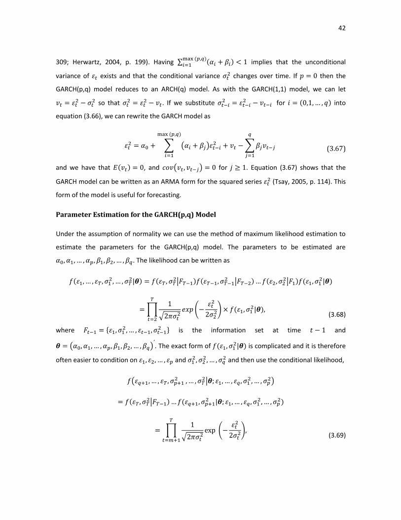
309; Herwartz, 2004, p. 199). Having implies that the unconditional

variance of exists and that the conditional variance changes over time. If then the

GARCH(p,q) model reduces to an ARCH(q) model. As with the GARCH(1,1) model, we can let

so that

. If we substitute

for into

equation (3.66), we can rewrite the GARCH model as

(3.67)

and we have that , and for . Equation (3.67) shows that the

GARCH model can be written as an ARMA form for the squared series (Tsay, 2005, p. 114). This

form of the model is useful for forecasting.

Parameter Estimation for the GARCH(p,q) Model


estimate the parameters for the GARCH(p,q) model. The parameters to be estimated are

. The likelihood can be written as

(3.68)

where

is the information set at time and

. The exact form of

is complicated and it is therefore

often easier to condition on and

and then use the conditional likelihood,

(3.69)

43

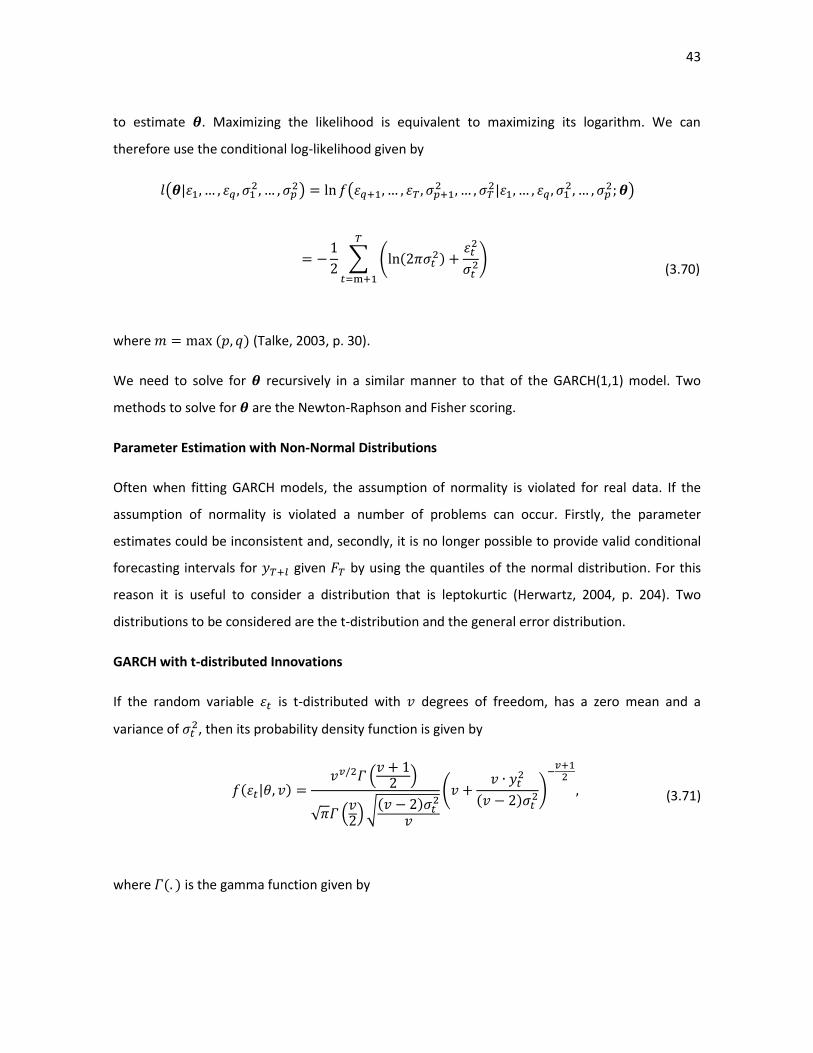
to estimate . Maximizing the likelihood is equivalent to maximizing its logarithm. We can

therefore use the conditional log-likelihood given by

(3.70)

where (Talke, 2003, p. 30).

We need to solve for recursively in a similar manner to that of the GARCH(1,1) model. Two

methods to solve for are the Newton-Raphson and Fisher scoring.

Parameter Estimation with Non-Normal Distributions

Often when fitting GARCH models, the assumption of normality is violated for real data. If the

assumption of normality is violated a number of problems can occur. Firstly, the parameter

estimates could be inconsistent and, secondly, it is no longer possible to provide valid conditional

forecasting intervals for given by using the quantiles of the normal distribution. For this

reason it is useful to consider a distribution that is leptokurtic (Herwartz, 2004, p. 204). Two

distributions to be considered are the t-distribution and the general error distribution.

GARCH with t-distributed Innovations

If the random variable is t-distributed with degrees of freedom, has a zero mean and a

variance of , then its probability density function is given by

(3.71)

where is the gamma function given by

44

(3.72)

The contribution of an observation to the log-likelihood function is given by

(3.73)

where is of the form given by (3.66) (Herwartz, 2004, p. 205). The log-likelihood is maximized in

the same manner as before.

GARCH with Generalized Error Distribution (GED)

A random variable with shape parameter , a mean of zero, and a variance has a probability

density function given by

(3.74)

where is given by

(3.75)

When , the probability density function is equal to the probability density function

and, when , the distribution becomes leptokurtic. The contribution of an observation to the

log-likelihood is given by

(3.76)

(Herwartz, 2004, pp. 205-206). Again, the log-likelihood is maximized as before.

45

Forecasting with the GARCH(p,q) Model

Forecasting with the GARCH model is similar to forecasting with an ARMA model. The forecast is

obtained by taking the conditional expectation. For the GARCH(p,q) model at forecast origin and

using the ARMA form of the model given by equation (3.67) the one step ahead forecast is given

by

(3.77)

where

and

are assumed to be known at time . In general, the

step ahead forecast is given by

(3.78)

where is given recursively by equation (3.78) for ,

for

, for and for (Shumway, 1988, pp. 142-

144; Shumway & Stoffer, 2006, pp. 116-117; Talke, 2003, pp. 30-31).

3.3 Extensions of the GARCH Model

The Integrated GARCH Model

The integrated GARCH (IGARCH) process was designed for the modeling of data that exhibit

persistent changes in volatility. An IGARCH process can either be a non-stationary process or a

stationary process with an infinite variance. A GARCH(p,q) process is stationary with a finite

variance if

(3.79)

If the polynomial in equation (3.67) has a unit root then the GARCH model is an IGARCH model.

The IGARCH model is a unit root GARCH model. The GARCH(p,q) process is called IGARCH if

(3.80)

46

(Ruppert, 2004, p. 377).

The IGARCH(1,1) model can be written as

(3.81)

(3.82)

where is defined as for the GARCH models and . When using the IGARCH model,

the unconditional variance no longer exists (Tsay, 2005, p. 122).

The Exponential GARCH Model

The exponential GARCH (EGARCH) model was first introduced by (Nelson, 1991). The model allows

for asymmetric effects between positive and negative asset returns. The EGARCH model has some

advantages over the GARCH model. Since the has been modeled then

will be positive

even if the model parameters are negative. This means that it's not necessary to impose

constraints on the parameters to force them to be non-negative (Brooks, 2008, p. 406; Ruppert,

2004, p. 383; Tsay, 2005, p. 124). Nelson considered the weighted innovation given by

(3.83)

where and are real constants and and are zero mean independent and

identically distributed sequences with continuous distributions. So, we have then that

. We can see the symmetry of if we rewrite it as

. (3.84)

The asymmetry of the EGARCH model means that if the relationship between the volatility and the

returns is negative then will be negative (Brooks, 2008, p. 406).

The EGARCH(p,q) model can be written as

(3.85)

(3.86)

47

where is a constant, is the back-shift operator, such that . The numerator,

and the denominator,

are polynomials with zeros

outside the unit circle (Tsay, 2005, p. 124).

Alternatively, the model can be written as

(3.87)

When the model is in the form of equation (3.87), we have that a positive contributes

to the log volatility and a negative contributes , where

. Thus the parameter is the leverage effect of (Tsay, 2005, p. 125). The

leverage effect occurs when returns become more volatile as the price decreases (Ruppert, 2004,

p. 384).

The GARCH-M Model

Engle, Lilien, and Robins (1987) first suggested the use of an ARCH-M model, which lets the

conditional variance of the return enter into the conditional mean equation. GARCH models,

however, have become more popular than ARCH models and it is, therefore, more common to

estimate a GARCH-M model (Brooks, 2008, p. 410). The M in GARCH-M stands for GARCH in the

mean. The GARCH-M model is useful when the return depends on its volatility (Tsay, 2005, p. 123).

The GARCH(1,1)-M model can be written as

(3.88)

(3.89)

(3.90)

where and are constants and the parameter is called the risk premium parameter. A positive

implies that the return is positively related to its volatility (Tsay, 2005, p. 123).

48

3.4 Testing for ARCH

To test for conditional heteroscedasticity, or ARCH effect, let be the residuals from the mean

equation for the return series. There are two tests that are commonly used to test for ARCH effect.

The first test makes use of the Ljung-Box statistics which are applied to the series

where the null hypothesis is that the first lags of the autocorrelation function of the series

are zero (Tsay, 2005, p. 101). The Ljung-Box statistic is given by

(3.91)

where is the sample size, is the number of lags, and is the estimate of the

autocorrelation of the squared residuals. is given by

(3.92)

where is the sample mean given by

(3.93)

Under the null hypothesis, is asymptotically distributed as a chi-squared distribution with

degrees of freedom (Box, Jenkins, & Reinsel, 2008, pp. 417-418; McLeod & Li, 1983, pp. 269-271).

The null hypothesis is rejected if , where

is the percentile of a

chi-squared distribution with degrees of freedom (Tsay, 2005, pp. 26-27).

The second test is the Lagrange multiplier test. The Lagrange multiplier test is equivalent to the

statistic for testing for in the regression

(3.94)

for , where is the error term, is a specified integer, and is the sample size

(Engle, 1982, p. 999; Lee, 1991, p. 266). The null hypothesis is then

49

Let

(3.95)

where

(3.96)

is the mean of , and let

(3.97)

where is the least squares residual from the regression in (3.94). Under the null hypothesis we

then have that

(3.98)

is asymptotically distributed as a chi-squared distribution with degrees of freedom. We reject

the null hypothesis if , where

is the upper percentile of a chi-

squared distribution with degrees of freedom, or if the p-value of is less than (Tsay, 2005,

pp. 101-102).

3.5 Model Selection Criteria

One of the difficulties that is often experienced when fitting models to data is that of choosing an

appropriate model. One of the reasons for this difficulty is that there are many different classes of

models to choose from (some of which have been discussed in the previous sections) and, within

each of those classes, there are a number of choices for the order of the model - for example the

choice of and for the GARCH(p,q) models. There are many different criteria that can be used to

aid in choosing the "best" possible model. However, the two most popular are to use the Akaike

information criteria (AIC) or the Bayesian information criteria (BIC). These criteria require the

estimation of a number of models and then the AIC and/or BIC values compared among the

50

estimated models. The model that has the minimum AIC or BIC value is then selected from those

models that have been estimated (Box, Jenkins, & Reinsel, 2008, pp. 211-212). The AIC and BIC are

calculated as follows:

(3.99)

(3.100)

where is the maximum likelihood for the model with parameters and is the size of the

sample. The disadvantage to using the AIC or BIC technique for model selection is that many

models need to be estimated by maximum likelihood, which can be time consuming and

computationally expensive (Box, Jenkins, & Reinsel, 2008, pp. 211-212).

3.6 Model Diagnostics

When the ARCH model has been properly specified then the standardized residuals, given by

(3.101)

form a sequence for independent and identically distributed random variables. The adequacy of

the fitted ARCH model can be checked by examining the series . The Ljung-Box statistics of

and can be used to check the adequacy of the mean equation and to test the validity of the

volatility equation respectively (Francq & Zakoian, 2010, p. 204). The skewness, kurtosis, and QQ-

plot of can be used to check if the distribution assumption is valid (Tsay, 2005, p. 109).

3.7 Multivariate ARCH and GARCH Models

When analyzing time series data it may become apparent that two or more series observed jointly

are dependent on each other. Increases or decreases in volatility in one series may result in

increases or decreases in one or more dependent series. This dependence leads to the extension

of the univariate ARCH and GARCH models to the multivariate case. Thus, we have MGARCH

models (Lutkepohl, 2006, p. 559).

51

3.7.1 Multivariate ARCH

Let be a K-dimensional zero mean, serially uncorrelated, process. The

process might be the residual process of some dynamic model and can be written as

(3.102)

where is a K-dimensional independent and identically distributed white noise, ,

and is the conditional covariance matrix of , given . The matrix,

, is

the symmetric positive definite square root of . The conditional distribution of the 's is of

the form

(3.103)

where . We have a multivariate ARCH(q) process if

(3.104)

where vech is the half vectorization operator which stacks the columns of a square matrix from

the diagonal downwards into a vector. is a

dimensional vector of constants and the

's are

coefficient matrices (Lutkepohl, 2006, p. 563).

The multivariate ARCH model has some technical problems that need to be addressed. One of

these problems is that the parameters need to have restrictions imposed to ensure that the

conditional covariance matrices are all positive definite. A model that ensures this

property is the BEKK model. The model is given by

(3.105)

where the 's are matrices. The are positive definite if

may be written in

product form

where

is a triangular matrix (Engle & Kroner, 1995; Lutkepohl, 2006,

p. 564).

52

3.7.2 Multivariate GARCH

The multivariate GARCH (MGARCH) model is a generalization of the multivariate ARCH model. The

MGARCH(p,q) model is given by

(3.106)

where the 's are fixed

matrices of coefficients (Gourieroux, 1997, p.

106; Lutkepohl, 2006, p. 564). As with the univariate GARCH model it is possible to express the

MGARCH model in the form of a multivariate ARMA (VARMA) form. To express the MGARCH in

VARMA form we let and . By substituting for

the MGARCH model can be written as

(3.107)

where for and for (Lutkepohl, 2006, p. 565).

Parameter Estimation

If in equation (3.101) so that the conditional distribution of given , is Gaussian

then using Bayes' theorem, the joint density function of is

(3.108)

Now, if the are observed values then the log-likelihood function for the MGARCH model given

by (3.106) is then

(3.109)

where is the vector of parameters to be estimated and

(3.110)

53

for . The initial values for are assumed to be known. We then estimate the

parameters by maximizing the log-likelihood using numerical methods. For the existence of a

unique maximum likelihood estimate it is important that an identified unique parameterization is

used. For example, the BEKK form of the model (Lutkepohl, 2006, p. 569).

Testing for ARCH

Before fitting an MGARCH model it is useful to check if there is a presence of ARCH effect in the

residuals. A Lagrange multiplier test can be used and we consider the model

(3.111)

where is a

dimensional matrix, the 's are

coefficient

matrices, and . The hypothesis to be tested is then

Let be the residual covariance estimate based on the model in (3.111) and let be the

corresponding matrix for . The test statistic

(3.112)

is asymptotically

distributed under the null hypothesis (Lutkepohl, 2006, p. 576).

We reject the null hypothesis for p-values less than our chosen significance level.

54

Chapter Four

4 Application of ARCH and GARCH Models

4.1 Introduction

This chapter will focus on the application of the ARCH and GARCH models to the data sets that

were introduced in Chapter 2. Hence, this chapter is a demonstration of theory applied to real

data.

The GARCH models were fitted using the PROC MODEL procedure which is readily available in SAS

software, Version 9.2 of the SAS System for Microsoft Windows. Copyright © 2002-2008 SAS

Institute Inc. SAS and all other SAS Institute Inc. product or service names are registered

trademarks or trademarks of SAS Institute Inc., Carry, NC, USA. Other software packages that can

be used to fit GARCH models include R, GAUSS FANPAC, and EVIEWS just to name a few. We will

focus our attention to fitting the GARCH models using SAS software. Code for selected models is

available in Appendix B.

4.2 Selecting the Best Model

The selection of the best model was based on the criteria of AIC, SBC, and where the smallest

AIC and/or SBC were selected as the best model and the largest was selected as the best

model. Other criteria for model selection were that the iteration procedure that was used to

estimate the model parameters had to converge, the parameter estimates should be significant

and the sum of the parameters and for and should not be larger

than 1.

4.3 Fitting the Model

Before fitting the ARCH and GARCH models, the first step is to remove any autocorrelation that is

present in the mean. This was achieved by fitting autoregressive models to the various data sets

using the number of lags indicated by the ACF and PACF of the return. The plots of the ACF and

PACF for the return of the four data sets used can be found in Chapter 2. Once an appropriate

autoregressive model has been selected we then proceed to fit the ARCH and GARCH models for

the residuals. It should be noted that the ARCH and GARCH models are fitted simultaneously with

the autoregressive model.

55

4.4 Analysis of the Anglo Gold Ashanti Ltd Data

The autoregressive model that was used to remove the autocorrelation present in the mean used

the order of 8. This was the lag suggested by the ACF and PACF in Figure 5. Once an appropriate

autoregressive model has been selected, the next step is to test for any ARCH disturbances using

the Q and LM tests for ARCH. The results of the Q and LM tests for ARCH disturbances can be seen

in Table 9. The Q and LM tests have highly significant p-values up to order 12 which shows that

there is ARCH effect present in the residuals.

Table 9: Anglo Gold Ashanti Q and LM Tests for ARCH Disturbances

Anglo Gold Ashanti Q and LM Tests for ARCH Disturbances

Order Q P-Value LM P-Value

1 159.2643 <0.0001 158.1438 <0.0001

2 264.2351 <0.0001 220.6881 <0.0001

3 327.7895 <0.0001 243.2753 <0.0001

4 404.7278 <0.0001 273.8361 <0.0001

5 461.3582 <0.0001 287.6571 <0.0001

6 522.8423 <0.0001 303.3927 <0.0001

7 548.4602 <0.0001 304.1659 <0.0001

8 596.5273 <0.0001 315.3790 <0.0001

9 628.8250 <0.0001 318.5491 <0.0001

10 650.1320 <0.0001 319.0574 <0.0001

11 677.3369 <0.0001 322.5036 <0.0001

12 706.6635 <0.0001 326.1557 <0.0001

After confirming that there is a significant ARCH effect, the next step is to fit the ARCH and GARCH

models to the data. To select the order for and we need to look at the ACF and PACF for the

squared residuals from the autoregressive model which can be seen in Figure 25.

56

Figure 25: ACF and PACF of Squared Residuals for the Anglo Gold Ashanti AR(8) Model

The ACF shows significant spikes at all lags and the PACF shows significant spikes from lags 1 to 8

and then a significant spike at lag 13. The ACF and PACF suggest that a GARCH(p,q) model would

be appropriate. To investigate this, ARCH(q) and GARCH(p,q) models were fitted where and

were allowed to vary from 1 to 13. The orders for and were also tested using the extensions to

the ARCH and GARCH model that were discussed in Chapter 3. The best models based on the AIC,

SBC and criteria, and the additional requirements of having significant parameter estimates,

are presented in Table 10. The parameter estimates for the three models were made using t-

distributed errors as this showed an improvement in the selection criteria compared to when

normally distributed errors were used.

Table 10: Anglo Gold Ashanti best models based on the three selection criteria

Model AIC SBC

GARCH(1,2) -4.6422 -4.6210 0.0064

GARCH(1,1) -4.6410 -4.6213 0.0063

ARCH(2) -4.5838 -4.6035 0.0069

57

The ARCH(2) Model

The ARCH(2) model was selected based on the highest value. This model also met the

additional criteria for selection in that the algorithm for parameter estimation converged, the sum

was less than 1 and the parameters were significant. The fit statistics for the ARCH(2) model can

be seen in Table 11 and the parameter estimates, along with their standard errors and p-values,

can be seen in Table 12. It can be seen that the sum is approximately 0.1934, which meets the

criteria for selection and it can also be seen that the ARCH terms are highly significant with p-

values less than 0.0001.

Table 11: Fit Statistics for the ARCH(2) Model

AIC -4.5838

SBC -4.6035

0.0069

SSE 2.8178

MSE 0.0007

Log Likelihood 9650.4420

MAE 0.9576

MAPE 61.6188

58

Table 12: Parameter Estimates with Standard Errors and p-values for the ARCH(2) Model

Parameter Estimate Standard Error P-Value

Intercept -0.0007 0.0003 0.0451

AR(1) 0.0552 0.0165 0.0008

AR(2) -0.0162 0.0163 0.3214

AR(3) -0.0144 0.0145 0.3185

AR(4) 0.0166 0.0143 0.2477

AR(5) 0.0018 0.0140 0.8954

AR(6) -0.0033 0.0140 0.8168

AR(7) -0.0227 0.0140 0.1062

AR(8) -0.0315 0.0142 0.0269

0.0003 0.00002 <0.0001

0.1089 0.0177 <0.0001

0.0845 0.0154 <0.0001

Degrees of Freedom 4.4789 0.3640 <0.0001

The GARCH(1,1) Model

The GARCH(1,1) model was the one having the smallest SBC value. The additional criteria for

selection was that the algorithm for parameter estimation should converge, the sum of and

should be less than 1 and the parameters should be significant. The fit statistics for the

GARCH(1,1) model can be found in Table 13 and the parameter estimates along with their

standard error and p-values can be seen in Table 14. It can be seen that the sum of and is

approximately 0.9559 which meets the criteria for selection and it can also be seen that the ARCH

and GARCH terms are highly significant with p-values less than 0.001.

59

Table 13: Fit Statistics for the GARCH(1,1) Model

AIC -4.6410

SBC -4.6213

0.0063

SSE 2.8195

MSE 0.0007


MAE 0.9211

MAPE 61.1245

Table 14: Parameter Estimates with Standard Errors and p-values for the GARCH(1,1) Model


Intercept -0.0008 0.0003 0.0180

AR(1) 0.0610 0.0155 <0.0001

AR(2) -0.0086 0.0163 0.5996

AR(3) -0.0264 0.0153 0.0841

AR(4) 0.0135 0.0158 0.3927

AR(5) 0.0005 0.0177 0.9797

AR(6) -0.0096 0.0151 0.5264

AR(7) -0.0291 0.0148 0.0500

AR(8) -0.0230 0.0151 0.1289

0.000009 0.000003 0.0052

0.0440 0.0088 <0.0001

0.9119 0.0185 <0.0001


60


The GARCH(1,2) Model was selected based on having the smallest AIC value. The additional

criteria for selection were that the algorithm for parameter estimation should converge, the sum

of and should be less than 1 and the parameters should be significant. The fit statistics for

the GARCH(1,2) model can be found in Table 15 and the parameter estimates along with their

standard errors and p-values can be found in Table 16. It can be seen that the sum of and is

approximately 0.9719 which meets the criteria for selection and it can also be seen that the ARCH

and GARCH terms are significant with having a p-value of 0.0081, having a p-value of 0.0004,

having a p-value of 0.0338 and having a p-value less than 0.0001.


AIC -4.6422

SBC -4.6210

0.0064

SSE 2.8193

MSE 0.0007


MAE 0.9195

MAPE 60.5263

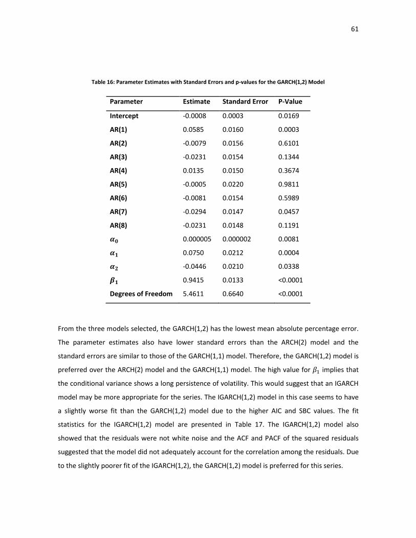
61



Intercept -0.0008 0.0003 0.0169

AR(1) 0.0585 0.0160 0.0003

AR(2) -0.0079 0.0156 0.6101

AR(3) -0.0231 0.0154 0.1344

AR(4) 0.0135 0.0150 0.3674

AR(5) -0.0005 0.0220 0.9811

AR(6) -0.0081 0.0154 0.5989

AR(7) -0.0294 0.0147 0.0457

AR(8) -0.0231 0.0148 0.1191

0.000005 0.000002 0.0081

0.0750 0.0212 0.0004

-0.0446 0.0210 0.0338

0.9415 0.0133 <0.0001


From the three models selected, the GARCH(1,2) has the lowest mean absolute percentage error.

The parameter estimates also have lower standard errors than the ARCH(2) model and the

standard errors are similar to those of the GARCH(1,1) model. Therefore, the GARCH(1,2) model is

preferred over the ARCH(2) model and the GARCH(1,1) model. The high value for implies that

the conditional variance shows a long persistence of volatility. This would suggest that an IGARCH

model may be more appropriate for the series. The IGARCH(1,2) model in this case seems to have

a slightly worse fit than the GARCH(1,2) model due to the higher AIC and SBC values. The fit

statistics for the IGARCH(1,2) model are presented in Table 17. The IGARCH(1,2) model also

showed that the residuals were not white noise and the ACF and PACF of the squared residuals

suggested that the model did not adequately account for the correlation among the residuals. Due

to the slightly poorer fit of the IGARCH(1,2), the GARCH(1,2) model is preferred for this series.

62

Table 17: Fit Statistics for the IGARCH(1,2) Model

AIC -4.6178

SBC -4.5982

0.0068

SSE 2.8182

MSE 0.0007


MAE 0.8086

MAPE 54.2345

Finally, to ensure that the GARCH(1,2) model is adequate we look at the ACF and PACF of the

residuals and the squared residuals and perform the Q and LM tests for ARCH disturbances to

determine if the ARCH effect has been accounted for. The plots of the ACF and PACF of residuals

can be seen in Figure 26. These plots show that the model for the mean is adequate.

Figure 26: ACF and PACF of Residuals for the GARCH(1,2) Model

The plots of the ACF and PACF of squared residuals can be seen in Figure 27. These plots show that

the GARCH(1,2) model adequately accounts for the serial correlation that was present in the

residuals.

63

Figure 27: ACF and PACF of Squared Residuals for the GARCH(1,2) Model

The results of the Q and LM test for ARCH disturbances when the GARCH(1,2) model was used can

be found in Table 18. These results show that there is no longer any significant ARCH effect.

Table 18: Anglo Gold Ashanti Testing for ARCH Disturbances after fitting the GARCH(1,2) Model

Anglo Gold Ashanti Q and LM Tests for ARCH Disturbances After Fitting the GARCH(1,2) Model


1 0.6121 0.4340 0.6670 0.4141

2 3.1411 0.2079 3.0635 0.2162

3 3.6954 0.2963 3.6317 0.3041

4 5.0413 0.2831 4.8761 0.3002

5 5.2328 0.3881 5.0965 0.4042

6 5.2655 0.5102 5.1030 0.5307

7 5.8483 0.5576 5.7247 0.5722

8 5.8543 0.6636 5.7455 0.6757

9 7.5938 0.5755 7.4335 0.5921

10 9.0038 0.5317 8.9403 0.5378

11 9.2260 0.6010 9.1229 0.6105

12 9.4968 0.6600 9.3390 0.6737

64

4.5 Analysis of the DRD Gold Ltd Data

To remove the autocorrelation that was present in the mean an autoregressive model was fitted

with a lag of 1 which was revealed by the ACF and PACF of the return. The ACF and PACF of the

return can be seen in Figure 11. The next step is to test for ARCH disturbances using the Q and LM

tests. The results for the Q and LM tests can be seen in Table 19. The results of the test for ARCH

disturbances show that there is a presence of a significant ARCH effect with p-values less than

0.0001.

Table 19: DRD Gold Q and LM Tests for ARCH Disturbances

DRD Gold Q and LM Tests for ARCH Disturbances


1 19.0408 <0.0001 19.0372 <0.0001

2 34.7043 <0.0001 32.5279 <0.0001

3 47.0399 <0.0001 41.6831 <0.0001

4 51.1761 <0.0001 43.6747 <0.0001

5 52.4679 <0.0001 43.9888 <0.0001

6 53.6468 <0.0001 44.3963 <0.0001

7 55.3334 <0.0001 45.2898 <0.0001

8 59.6821 <0.0001 48.3487 <0.0001

9 61.1163 <0.0001 48.8935 <0.0001

10 62.6868 <0.0001 49.5154 <0.0001

11 63.1498 <0.0001 49.5567 <0.0001

12 64.9216 <0.0001 50.4765 <0.0001

The next step is to fit ARCH and GARCH models to the series. The ACF and PACF of the squared

residuals shown in Figure 28 indicate that the orders for and could range from 1 to 3.

65

Figure 28: ACF and PACF of Squared Residuals for the DRD Gold AR(1) Model

A number of ARCH(q) and GARCH(p,q) models were fitted where both and were allowed to

vary between 1 and 3. The extensions for the ARCH and GARCH models discussed in Chapter 3

were also tested. The best models based on the AIC, SBC, and criteria and the additional

criteria of having significant parameter estimates are presented in Table 20. These models were

fitted using the t-distribution for the errors as this resulted in an improved fit compared to when

normally distributed errors were used.

Table 20: DRD Gold best models based on the three selection criteria

Model AIC SBC

GARCH(3,3) -3.9007 -3.8855 0.0001

ARCH(3) -3.8739 -3.8633 0.0002


The GARCH(3,3) model was selected based on having the smallest AIC and the smallest SBC. The

model also met the additional requirements for selection; these requirements being that the

algorithm for parameter estimation should converge, the sum of and should be less than 1

and the parameters should be significant. The fit statistics for the GARCH(3,3) model can be found

in Table 21 and the parameter estimates along with their standard errors and p-values can be seen

in Table 22. The estimates of the parameters show that the sum of the and terms is

66

approximately 0.7378 which meets the criteria for models selection and the p-values for the

estimates shows significance for all the GARCH terms except for the term, which has a p-value

of 0.6452. Having significance for the majority of the parameters satisfies the requirements for

model selection.

Table 21: Fit Statistics for the GARCH(3,3)

AIC -3.9007

SBC -3.8855

0.0001

SSE 7.1786

MSE 0.0017


MAE 1.1591

MAPE 45.8011



Intercept -0.0013 0.0004 0.0008

AR(1) 0.0084 0.0142 0.5552

0.00003 0.00001 0.0091

0.0630 0.0088 <0.0001

0.0356 0.0069 <0.0001

0.0547 0.0080 <0.0001

-0.1311 0.0197 <0.0001

-0.0132 0.0286 0.6452

0.7288 0.0336 <0.0001


67

The ARCH(3) Model

The ARCH(3) model was selected based on having the largest value. The algorithm for

parameter estimation converged, the sum of the was less than 1 and the parameters were

significant which meets the additional criteria for model selection. The fit statistics for the ARCH(3)

model can be seen in Table 23 and the parameter estimates, along with their standard errors and

p-values, are given in Table 24. The estimates for the parameters shows that the sum of the is

approximately 0.2539, which meets the criteria for model selection. The parameters are also all

significant with p-values <0.0001.

Table 23: Fit Statistics for the ARCH(3) Model

AIC -3.8739

SBC -3.8633

0.0002

SSE 7.1782

MSE 0.0017


MAE 1.1379

MAPE 44.5570

Table 24: Parameter Estimates with Standard Errors and p-values for the ARCH(3) Model


Intercept -0.0015 0.0004 0.0001

AR(1) 0.0145 0.0151 0.3379

0.0003 0.00002 <0.0001

0.0927 0.0148 <0.0001

0.0597 0.0118 <0.0001

0.1015 0.0155 <0.0001

Degrees of Freedom 2.5498 0.1379 <.0001

68

The GARCH(3,3) model and the ARCH(3) model both have goodness of fit statistics that are very

similar, thereby making a choice between the two models difficult. Both models showed that they

have adequately accounted for the presence of any ARCH effect based upon the Q and LM tests

for ARCH effect. When performing diagnostic checks using the ACF and PACF for residuals and

squared residuals, the GARCH(3,3) model had slightly better results than the ARCH(3) model.

Therefore, the GARCH(3,3) model is preferred for this data. The GARCH(3,3) model shows a fairly

high value for which suggests that there is some persistence in the volatility. The plots of the

ACF and PACF of residuals for the GARCH(3,3) model can be seen in Figure 29. These plots show

that the model for the mean is adequate.


The plots of the ACF and PACF of squared residuals can be seen in Figure 30. These plots show that

the GARCH(3,3) model has removed the autocorrelation that was present in the residuals.

69


Finally, the Q and LM tests for ARCH disturbances is performed to confirm that the model has

removed the effect of ARCH. The results are shown in Table 25, where it is seen that the ARCH

effect has been removed.

Table 25: DRD Gold Testing for ARCH Disturbances after fitting the GARCH(3,3) Model

DRD Gold Q and LM Tests for ARCH Disturbances After Fitting the GARCH(3,3) Model


1 0.0967 0.7558 0.0966 0.7560

2 0.1900 0.9094 0.1905 0.9091

3 0.2846 0.9629 0.2865 0.9625

4 0.3634 0.9854 0.3673 0.9851

5 0.4072 0.9951 0.4131 0.9950

6 0.4965 0.9979 0.5054 0.9978

7 0.6076 0.9989 0.6206 0.9989

8 0.6623 0.9996 0.6790 0.9996

9 0.7628 0.9998 0.7849 0.9998

10 0.8049 0.9999 0.8312 0.9999

11 0.8479 1.0000 0.8793 1.0000

12 0.8993 1.0000 0.9365 1.0000

70

4.6 Analysis of the Gold Fields Ltd Data

To remove the autocorrelation that was present in the mean, autoregressive model of order 8 was

fitted to the return series. The next step is to test for ARCH disturbances using the Q and LM tests.

The results for the tests are displayed in Table 26, where it can be seen that there is a significant

ARCH effect with p-values less than 0.0001.

Table 26: Gold Fields Q and LM Tests for ARCH Disturbances

Gold Fields Q and LM Tests for ARCH Disturbances


1 26.4052 <0.0001 26.3904 <0.0001

2 33.8876 <0.0001 31.5257 <0.0001

3 44.7877 <0.0001 39.6443 <0.0001

4 52.8998 <0.0001 44.4776 <0.0001

5 73.4160 <0.0001 59.3077 <0.0001

6 81.6116 <0.0001 62.5790 <0.0001

7 84.5293 <0.0001 63.1511 <0.0001

8 86.9437 <0.0001 63.5969 <0.0001

9 97.1018 <0.0001 69.2363 <0.0001

10 104.1206 <0.0001 71.6462 <0.0001

11 108.2553 <0.0001 72.6694 <0.0001

12 111.2771 <0.0001 73.2931 <0.0001

We next need to select the order for and for the GARCH model. The ACF and PACF of the

squared residuals shown in Figure 31 from the AR(8) model indicate that the order for and

could vary from 1 to 5.

71

Figure 31: ACF and PACF of Squared Residuals for the Gold Fields AR(8) Model

ARCH(q) and GARCH(p,q) models were fitted where and were allowed to vary between 1 and

5. The extensions for the GARCH model discussed in Chapter 3 were also tested. The best model

based on the AIC, SBC, and criteria and the additional requirements of having significant

parameter estimates are presented in Table 27. For the Gold Fields data, the GARCH(1,2) model

had the best AIC, SBC, and values. The model was fitted simultaneously with the autoregressive

model and the t-distribution was used for the errors as this provided better results than when the

normal distribution was used.

Table 27: Gold Fields best models based on the three selection criteria

Model AIC SBC

GARCH(1,2) -4.1958 -4.1687 0.0058


The GARCH(1,2) model met the additional criteria for selection in that the sum of and was

less than 1, the algorithm for parameter estimation converged and the parameter estimates were

significant. The fit statistics for the GARCH(1,2) model can be seen in Table 28 and the parameter

estimates with standard errors and p-values can be found in Table 29. The parameter estimates

for the GARCH(1,2) model are all significant with p-values less than 0.05. It is also noted that the

72

sum of and is approximately 0.9744, which meets the criteria for selection. The high value

for suggests that there is persistence in the volatility for the Gold Fields data.


AIC -4.1958

SBC -4.1687

0.0058

SSE 3.6476

MSE 0.0012


MAE 0.9113

MAPE 45.8793



Intercept -0.0004 0.0005 0.4329

AR(1) 0.0482 0.0188 0.0103

AR(2) -0.0287 0.0176 0.1043

AR(3) -0.0045 0.0221 0.8402

AR(4) 0.0118 0.0174 0.4988

AR(5) 0.0048 0.0188 0.7966

AR(6) 0.0098 0.0180 0.5851

AR(7) -0.0342 0.0175 0.0504

AR(8) -0.0091 0.0200 0.6523

0.00001 0.000002 0.0056

0.0732 0.0192 0.0001

-0.0407 0.0198 0.0401

0.9419 0.0120 <.0001

Degrees of Freedom 5.9644 0.9277 <.0001

73

From the parameter estimates the sum of and is close to 1, which suggests that an

IGARCH(1,2) model might be more appropriate. The IGARCH(1,2) model was fitted to investigate

this and it is seen that the model has a slightly poorer fit than the GARCH(1,2) model. This is shown

by the AIC, SBC, and values. Therefore, the IGARCH(1,2) model will not be considered. The

goodness of fit statistics for the IGARCH(1,2) model can be found in Table 30.

Table 30: Fit Statistics for the IGARCH(1,2) Model

AIC -4.1719

SBC -4.1467

0.0057

SSE 3.6479

MSE 0.0012


MAE 0.8010

MAPE 41.3779

Finally, to ensure that the GARCH(1,2) model is appropriate, we look at the ACF and PACF of the

residuals and squared residuals. The plots of the ACF and PACF for the residuals can be seen in

Figure 32. The two plots show that the model for the mean is satisfactory.


74

The plots of the ACF and PACF of the squared residuals can be seen in Figure 33. The two plots

show that the GARCH(1,2) model has removed the serial correlation that was present and,

therefore, this model is adequate. This is confirmed by the Q and LM tests which show that there

is no longer any ARCH effect. The results for the tests can be found in Table 31.


Table 31: Gold Fields Testing for ARCH Disturbances after fitting the GARCH(1,2) Model

Gold Fields Q and LM Tests for ARCH Disturbances After Fitting the GARCH(1,2) Model


1 0.0006 0.9802 0.0006 0.9808

2 0.1074 0.9477 0.1060 0.9484

3 0.1884 0.9794 0.1845 0.9801

4 0.2618 0.9921 0.2544 0.9926

5 0.2763 0.9981 0.2706 0.9982

6 0.3434 0.9993 0.3415 0.9993

7 0.4337 0.9997 0.4337 0.9997

8 0.7099 0.9995 0.7075 0.9995

9 0.8317 0.9997 0.8244 0.9997

10 0.9712 0.9998 0.9549 0.9999

11 1.1167 0.9999 1.0909 0.9999

12 1.2341 1.0000 1.2000 1.0000

75

4.7 Analysis of the Harmony Gold Mining Company Ltd Data

The ACF and PACF of the return series pointed towards the fact that a lag of 2 be used for the

autoregressive model to remove the autocorrelation present in the mean. The next step is to test

for ARCH disturbances using the Q and LM tests. The results of the test can be seen in Table 32

where the p-values show that there is a significant ARCH effect.

Table 32: Harmony Gold Mining Company Q and LM Tests for ARCH Disturbances

Harmony Gold Mining Company Q and LM Tests for ARCH Disturbances


1 164.2102 <0.0001 163.6975 <0.0001

2 211.4164 <0.0001 183.1611 <0.0001

3 240.2676 <0.0001 193.9065 <0.0001

4 259.5541 <0.0001 199.6437 <0.0001

5 288.2871 <0.0001 212.2479 <0.0001

6 315.9061 <0.0001 221.2664 <0.0001

7 349.1310 <0.0001 232.7901 <0.0001

8 371.9450 <0.0001 237.0479 <0.0001

9 394.2524 <0.0001 241.9868 <0.0001

10 405.9873 <0.0001 242.6749 <0.0001

11 417.5543 <0.0001 244.1003 <0.0001

12 443.6512 <0.0001 252.7311 <0.0001

We next select the orders for and for the ARCH(q) and GARCH(p,q) models. The ACF and PACF

of the squared residuals from the AR(2) model, seen in Figure 34, suggested that orders from 1 to

7 might be useful.

76

Figure 34: ACF and PACF of Squared Residuals for the Harmony Gold Mining Company AR(2) Model

The best models based on the AIC, SBC, and criteria, along with the additional requirements of

having significant parameter estimates, can be seen in Table 33. The parameter estimates for the

two models presented were fitted using the t-distribution for the errors, as this provided better

results than models fitted with the normal distribution.

Table 33: Harmony Gold Mining Company best models based on the three selection criteria

Model AIC SBC

GARCH(2,1) -4.2889 -4.2768 0.0060

GARCH(1,4) -4.2916 -4.2765 0.0060


The GARCH(2,1) model was selected based on having the best SBC value. The model also met the

additional requirements in that the sum of and was less than 1, the parameter estimates

were significant and the algorithm for the estimation of the parameters converged. The fit

statistics for the GARCH(2,1) model can be found in Table 34 and the parameter estimates, along

with their standard errors and p-values, can be seen in Table 35. It can be seen that the sum of

and is approximately 0.9227, which meets the criteria for selection and, in addition the

parameters for the GARCH model, are all significant with p-values less than 0.01.

77


AIC -4.2889

SBC -4.2768

0.0060

SSE 4.2810

MSE 0.0010


MAE 0.9842

MAPE 52.0703



Intercept -0.0008 0.0004 0.0297

AR(1) 0.0637 0.0152 <0.0001

AR(2) -0.0109 0.0141 0.4406

0.00001 0.000004 0.0064

0.0692 0.0102 <0.0001

0.1728 0.0652 0.0081

0.6807 0.0669 <0.0001



The GARCH(1,4) model was selected based on having the best AIC value. The additional

requirements of having convergence of the algorithm for parameter estimations, significant

parameter estimates and the sum of and being less than 1 were also met. The fit statistics for

the GARCH(1,4) can be seen in Table 36 and the parameter estimates, along with their standard

errors and p-values, can be found in Table 37. The parameter estimates for is not significant

with a p-value of 0.0724. The remaining parameter estimates for the GARCH(1,4) model are

78

significant with p-values less than 0.05. The additional criteria for selection has also been met in

that the sum of and is approximately 0.9782.


AIC -4.2916

SBC -4.2765

0.0060

SSE 4.2811

MSE 0.0010


MAE 0.9805

MAPE 51.8924



Intercept -0.0008 0.0004 0.0384

AR(1) 0.0631 0.0155 <0.0001

AR(2) -0.0096 0.0152 0.5263

0.000002 0.000001 0.0724

0.0900 0.0176 <0.0001

-0.0624 0.0227 0.0060

0.0449 0.0204 0.0281

-0.0506 0.0157 0.0013

0.9563 0.0090 <0.0001


Both the GARCH(2,1) and the GARCH(1,4) model have similar MAPE and MAE values and both

have the same value. Therefore, in choosing the final model the more parsimonious model is

selected. Therefore, the GARCH(2,1) model is preferred. The parameter estimate for is

79

relatively large which shows that there is some persistence in the volatility for the Harmony data.

To ensure that the model is adequate, we look at the ACF and PACF of the residuals and the

squared residuals. The ACF and PACF of the residuals can be seen in Figure 35. The plots show that

the autoregressive model has removed any correlation present in the mean.


The plots of the ACF and PACF of the squared residuals can be seen in Figure 36. The plots show

that the GARCH(2,1) has been successful in removing the serial correlation present in the

residuals.


80

As a final test the Q and LM tests for ARCH effect are performed and it is shown that there is no

remaining ARCH effect. Therefore, the GARCH(2,1) model was useful in accounting for the

presence of ARCH effect. The results for the Q and LM tests are displayed in Table 38.

Table 38: Harmony Gold Mining Company Testing for ARCH Disturbances after fitting the GARCH(2,1) Model

Harmony Gold Mining Company Q and LM Tests for ARCH Disturbances


1 0.6834 0.4084 0.6709 0.4127

2 1.0047 0.6051 1.0093 0.6037

3 1.4901 0.6846 1.5110 0.6797

4 3.2648 0.5145 3.3461 0.5017

5 5.9307 0.3130 5.8506 0.3210

6 5.9792 0.4255 5.8932 0.4353

7 6.4816 0.4848 6.3827 0.4958

8 7.2526 0.5096 7.1954 0.5157

9 7.2671 0.6093 7.2412 0.6120

10 9.2587 0.5077 9.2492 0.5086

11 11.2453 0.4229 11.2817 0.4200

12 11.2578 0.5070 11.3005 0.5034

81

Chapter Five

5 Stochastic Volatility Models

An alternative family of models to the ARCH/GARCH family of models for modeling the volatility of

a financial time series are the Stochastic Volatility models. The difference between the

ARCH/GARCH models and the Stochastic Volatility models is that the ARCH models are observation

driven, whereas the Stochastic Volatility models are parameter driven. Stochastic volatility models

model the conditional variance as an unobserved component that follows some underlying latent

stochastic process (Mahieu & Schotman, 1998, p. 333). The conditional variance is modeled by

introducing an error or innovation term to the conditional variance equation of . The resulting

model is called a Stochastic Volatility model. Despite having some theoretical advantages,

Stochastic Volatility models have not been as widely used as the ARCH/GARCH models. This is

mainly due to the fact that, unlike the ARCH/GARCH models, the likelihood is complicated and

often difficult to evaluate (Shimada & Tsukuda, 2005, p. 3).

5.1 The Stochastic Volatility Model

A Stochastic Volatility model is defined as

(5.1)

(5.2)

where the are , the are , and are independent, is a

constant, and all the zeros of the polynomial

are greater than 1 in modulus (Tsay,

2005, p. 134).

The addition of the innovation increases the flexibility of the model in describing the evolution

of the volatility but, at the same time, increases the difficulty in estimating model parameters. This

difficulty is due to the fact that for each shock , the model makes use of two innovations, and

. Estimating Stochastic Volatility models is done using a quasi-likelihood method with results

from a state-space model together with the use of the Kalman filter (Tsay, 2005, p. 134). Monte

82

Carlo methods can also be used to estimate Stochastic Volatility models. This dissertation will

focus on the quasi-likelihood method.

5.2 State-Space Models

State-space models offer an approach to time series analysis that can simplify maximum likelihood

estimation and the handling of missing data (Tsay, 2005, p. 490). The general form of the linear

state-space model is given by

(5.3)

(5.4)

Equation (5.3) is known as the state equation. The state equation is used to generate from the

previous states , where for and . It is assumed that the

are independent and identically distributed normal vectors with a mean of the zero vector

and covariance matrix , whilst is a transition matrix. Equation (5.4) is known as the

observation equation. The observation equation is needed because it is not possible to observe

the state vector directly. The observation equation gives a linear transformation of the state

vector with added noise. is known as the observation matrix and it has dimension ,

is a vector of observations which has dimension . is assumed to be Gaussian white noise

with a covariance matrix . When using state-space models it is generally assumed that the

process starts with a vector that is normal with mean and covariance matrix

(Shumway & Stoffer, 2000, p. 306).

We make inference about the state from the data and the model. Three types

of inference that are commonly used are filtering, prediction and smoothing. Filtering means to

update the state variable given all the information at time . Prediction means to forecast the

state variable, that is, forecast for given all the information at time , where is the

forecast origin. Smoothing means to estimate the state variable given the information available

at time where (Tsay, 2005, pp. 493-494).

We will use the following definitions for the derivations of the Kalman Filter and Kalman

Smoother:

83

(5.5)

and

(5.6)

respectively.

When , then will be written as

. The derivation of the Kalman filter and Kalman

smoother relies on the assumption of normality. This will also mean that equation (5.6) is the

conditional error covariance given by

It should be noted that the covariance matrix between and is zero for any and .

Due to the assumption of normality this implies that and are independent (Shumway

& Stoffer, 2006, p. 330).

5.3 The Kalman Filter

The purpose of the Kalman filter is to update the state variable recursively as new data becomes

available. The Kalman filter is used to update the filter from to

when a new is observed.

The Kalman filter is derived as follows.

From equation (5.5) and using (5.3) we have

(5.7)

and from (5.6)

(5.8)

84

We next define the innovations as

(5.9)

for .

Now,

(5.10)

and

(5.11)

We also have that for . This implies that the innovations are

independent of the past observations because the innovations follow a Gaussian process

(Shumway & Stoffer, 2000, pp. 313-314). The covariance between and conditional on is

(5.12)

The joint distribution of and conditional on is normal

(5.13)

We can now rewrite in the following way using Result 1 in Appendix A:

85

(5.14)

where

(5.15)

Using Result 1 in Appendix A we can calculate as

(5.16)

(Shumway & Stoffer, 2006, pp. 331-332).

For the state space model given by equations (5.3) and (5.4) using the initial conditions and

, for the Kalman filtering algorithm is given by

(5.17)

(5.18)

with

(5.19)

(5.20)

where

(5.21)

is known as the Kalman gain. Equations (5.17) and (5.18) are used for prediction when

with and

as initial conditions (Shumway & Stoffer, 2000, p. 313).

86

5.4 The Kalman Smoother

The purpose of smoothing is to estimate the state variable based on all the information

available. That is to estimate the state based on the sample , where (Tsay, 2005, p.

526). To derive the Kalman smoother we first define

(5.22)

and

(5.23)

where is an empty set and we let

(5.24)

for .

Now, since , , and are mutually independent, and and are independent,

we can use Result 1 in Appendix A to get

(5.25)

where

(5.26)

We next have that

(5.27)

because , , and lead to .

We then obtain the error covariance, , in the following way. Using equation (5.27) we have

(5.28)

87

(5.29)

(5.30)

Next, we multiply both sides of equation (5.30) by the transpose of itself and then take the

expectation to get

(5.31)

because the cross-product terms are zero. Now,

(5.32)

and

(5.33)

So, the Kalman smoother for the state-space model given by equations (5.3) and (5.4), with initial

conditions and

which are available from the Kalman filter is

(5.34)

(5.35)

where

(5.36)


5.5 The Lag One Covariance Smoother

The lag one covariance smoother is used to recursively obtain , which is defined by equation

(5.6) (Shumway & Stoffer, 2000, p. 319). We derive the lag one covariance smoother as follows:

88

We start by defining

(5.37)

Then, we use equations (5.19) and (5.21) to write

(5.38)

(5.39)

(5.40)

After expanding equation (5.40), and taking the expectation, we then have

(5.41)

We also have that

(5.42)

and

(5.43)

for any .

We now use equation (5.34) to get

(5.44)

and

(5.45)

89

Consequently, we multiply the left hand side of equation (5.44) by the transpose of the left hand

side of equation (5.45) and multiply the right hand side of equation (5.44) by the transpose of the

right hand side of equation (5.45). We then equate the two results and take the expectation. The

left hand side is then

(5.46)

while the right hand side is

(5.47)

The

can be written as

(5.48)

and we can write

as

(5.49)

For the state space model given by equations (5.3) and (5.4), where , for , and

are available from the Kalman filter and Kalman smoother. Using the initial condition

(5.50)

For , from equations (5.46) and (5.47) the lag one covariance smoother is

(5.51)


5.6 Maximum Likelihood Estimation

In order to use the Kalman filtering and smoothing equations, we need estimates of the

parameters that are used to specify the state space model given by equations (5.3) and (5.4). The

90

parameters are the initial mean , covariance , the transition matrix and the state and

observation covariance matrices and , respectively. These parameters are estimated using

maximum likelihood with the assumption that , and the errors and

are uncorrelated and jointly normal. To compute the likelihood, we use the innovations

defined by equation (5.9) as

(5.52)

and note that the innovations are a one-to-one linear transformation of the data .

We also note that the innovations are independent Gaussian random vectors with a mean of zero

and covariance defined by equation (5.11), as

Therefore we can write the log-likelihood as

(5.53)

where the constant has been ignored for simplicity and .

To maximize the log-likelihood in equation (5.53) we fix and then obtain a set of recursions for

the likelihood function and its first two derivatives. We can then use the Newton-Raphson

procedure to update the parameter values until the log-likelihood has been maximized. This

process can be summarized into the following four steps:

1. Select initial values for the parameters, .

2. Run the Kalman filter using the initial values, , to obtain a set of innovations and error

covariances.

3. Run iterations of the Newton-Raphson procedure to obtain new estimates for the

parameters.

91

4. Repeat Step 2 using the new parameter estimates obtained from Step 3 to generate a new

set of innovations and error covariances. Run Step 3. This process continues until the

difference between successive estimates of the parameters or the log-likelihood are small

enough.

5.7 The Expectation Maximization Algorithm

An alternative method to estimate the parameters for the state space model, given by equations

(5.3) and (5.4), is the expectation maximization (EM) algorithm. The EM algorithm consists of two

steps, the E-step and the M-step. The E-step, or expectation step, computes the expected value of

the complete data likelihood. The M-step, or maximization step, updates the parameter estimates

(Durbin & Koopman, 2001, p. 147; Xu & Wilke, 2007, p. 570). The idea behind the EM algorithm is

that along with the observations we are able to observe the states

. We could then take to be the complete data set having joint density

(5.54)

Under the assumption of normality, we can write the likelihood for the complete data as

(5.55)

(Shumway & Stoffer, 2000, p. 324).

The EM algorithm is used to obtain the maximum likelihood estimates of based on the

incomplete data given by . This is achieved by maximizing the conditional expectation of the

complete data likelihood. So, for iteration for the conditional expectation to be

maximized is

92

(5.56)

(Shumway & Stoffer, 1982, p. 256; Shumway & Stoffer, 2000, p. 324).

Given the parameters, , we can use the Kalman smoother to obtain conditional

expectations. This leads to

(5.57)

where

(5.58)

(5.59)

and

(5.60)

The present parameter values, , are used for the calculation of the smoothers in equations

(5.57), (5.58), (5.59) and (5.60) (Shumway & Stoffer, 1982, p. 257; Shumway & Stoffer, 2000, p.

325). The next step is the maximization step which involves minimizing equation (5.57) with

respect to the parameters at the iteration. The maximization step results in the following

updated estimates:

(5.61)

93

(5.62)

and

(5.63)

It is not possible to estimate the initial means and covariance simultaneously. The usual

convention is to fix both the mean and covariance, or just the covariance matrix, and then use

(5.64)

which is the estimator that is obtained from minimizing equation (5.57) under the assumption that

the covariance matrix has been fixed. The steps involved in the EM algorithm can be summarized

as follows:

1. Select the starting values for the parameters , and fix .

2. Compute the likelihood for the incomplete data as in equation (5.53).

3. Perform the E-Step of the algorithm using the Kalman filter and Kalman smoothing to

calculate given by equations (5.58), (5.59) and (5.60).

4. Perform the M-Step to update the estimates, and .

5. Repeat steps 2 to 4 until convergence has been achieved

(Shumway & Stoffer, 1982, p. 258; Shumway & Stoffer, 2000, p. 325).

94

5.8 The Stochastic Volatility Model

The stochastic volatility model is similar to the ARCH models, however, there is an added

stochastic noise term in the equation for . Recall from Chapter 3 that the GARCH (1,1) model is

given by

(5.65)

(5.66)

where . We now define

(5.67)

and

(5.68)

Then equation (5.66) can be written as

(5.69)

Equation (5.70) is the observation equation and , which is the stochastic variance is viewed as an

unobserved state process. The volatility process follows an autoregressive, AR(1), process such

that can be written as

(5.70)

where . The stochastic volatility model is then made up of equations (5.69) and

(5.70). To fit the stochastic volatility model, we keep the ARCH assumption of normality for .

With this normality assumption, we have that is distributed as the log of a chi-squared

random variable with one degree of freedom. The probability density function of is given by

(5.71)

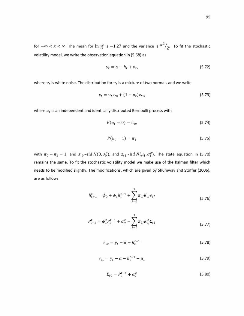
95

for . The mean for is and the variance is

. To fit the stochastic

volatility model, we write the observation equation in (5.68) as

(5.72)

where is white noise. The distribution for is a mixture of two normals and we write

(5.73)

where is an independent and identically distributed Bernoulli process with

(5.74)

(5.75)

with , and , and

. The state equation in (5.70)

remains the same. To fit the stochastic volatility model we make use of the Kalman filter which

needs to be modified slightly. The modifications, which are given by Shumway and Stoffer (2006),

are as follows

(5.76)

(5.77)

(5.78)

(5.79)

(5.80)

96

(5.81)

(5.82)

(5.83)

Equations (5.76) to (5.83) are the filtering equations for the model given by equations (5.70) and

(5.72). The probabilities given by for need to be assessed to

use the filtering equations. Once has been obtained, we can determine since

. To find let be the conditional density of given , and for

. Then using Bayes rule we have

(5.84)

If there is no reason to prefer one state, then letting

is sufficient. The exact values for

are difficult to obtain and, therefore, we choose to approximate by using

the normal distribution with mean and variance for and . The model

parameters to be estimated are given by

and are estimate by

maximum likelihood using the likelihood

(5.85)

where is approximated as

. The likelihood can be maximized as a

function of the parameters by using a Newton method, or the EM algorithm could be used when

considering the complete data likelihood (Shumway & Stoffer, 2006, pp. 388-390).

97

Chapter Six

6 Application of Stochastic Volatility Models

6.1 Introduction

This chapter focuses on the application of the stochastic volatility model discussed in Chapter 5 to

the data that was introduced in Chapter 2. The stochastic volatility model makes use of the

logarithm of the squared residuals from an ARMA model instead of the residuals themselves. This

has the potential to create a problem if any of the residuals are zero. If there are residuals that are

zero it is possible to deal with this problem by adding a positive constant to the residuals to ensure

that there are no zero values. The resulting transformation is where is a small positive

constant. The stochastic volatility model is then applied to the data using the logarithm of the

squared transformed residuals which is given by

For all the data sets that were modeled there was no problem with having any zero values for the

residuals and therefore no transformation was applied. The software that was used to fit the

model was R: A Language and Environment for Statistical Computing (2010) and this software is

freely available for download from http://cran.r-project.org/. The code for the stochastic volatility

model can be found in Appendix B.

The stochastic volatility model is now fitted to the Anglo Gold Ashanti Ltd, DRD Gold Ltd, Gold

Fields Ltd and Harmony Gold Mining Company Ltd data. The value for was fixed at 0.5. The

estimation procedure used a Newton method to maximize the likelihood in equation (5.85).

6.2 Stochastic Volatility Model for the Anglo Gold Ashanti Ltd Data

The stochastic volatility model is fitted to the residuals from the AR(8) model for the return. The

parameter estimates for the model are presented in Table 39. The parameter estimate for is

high, which suggests that there is long persistence of volatility. This persistence of volatility was

also seen in the results of the GARCH(1,2) model for the Anglo Gold Ashanti data, which can be

seen in Chapter 4.

98

Table 39: Parameter Estimates for the Anglo Gold Ashanti Stochastic Volatility Model

Parameter Estimate Standard Error

-0.0045 0.0377

0.9776 0.0117

0.1524 0.0431

-7.5696 1.6739

1.1094 0.0425

-2.7462 0.1304

2.8034 0.0739

6.3 Stochastic Volatility Model for the DRD Gold Ltd Data

The stochastic volatility model is applied to the residuals from the AR(1) model for the DRD Gold

data. The parameter estimates for the stochastic volatility model can be seen in Table 40. It can be

seen that the estimate for is high, which indicates that the volatility has long persistence. The

GARCH(3,3) model for the DRD Gold data from Chapter 4 also showed that the volatility had long

persistence.

Table 40: Parameter Estimates for the DRD Gold Stochastic Volatility Model


0.2022 0.1907

0.9556 0.0225

0.2835 0.0773

-11.5412 2.2561

1.1275 0.0562

-4.1948 0.1563

3.3315 0.0909

99

6.4 Stochastic Volatility Model for the Gold Fields Ltd Data

The stochastic volatility model is fitted to the residuals from the AR(8) Model for the return of the

Gold Fields data. The parameter estimates for the stochastic volatility model are displayed in Table

41. The parameter estimate for is high, which indicates that the volatility has long persistence.

This long persistence of volatility was also seen for the GARCH(1,2) model for the Gold Fields data,

which can be found in Chapter 4.

Table 41: Parameter Estimates for the Gold Fields Stochastic Volatility Model


-0.0145 0.0209

0.9896 0.0056

0.1208 0.0282

-5.8841 1.8978

1.0525 0.0435

-2.8402 0.1411

2.6824 0.0813

6.5 Stochastic Volatility Model for the Harmony Gold Mining Company Ltd Data

The stochastic volatility model is applied to the residuals of the AR(2) model for the return. The

parameter estimates for the stochastic volatility model can be found in Table 42. The estimate for

is high, which indicates that the volatility remains persistent for a long period. This volatility

persistence was also seen for GARCH(2,1) model for the Harmony Gold data from Chapter 4.

100

Table 42: Parameter Estimates for the Harmony Gold Stochastic Volatility Model


0.0092 0.0601

0.9708 0.0127

0.2214 0.0530

-7.6774 2.0463

1.0699 0.0485

-3.5393 0.1394

3.1758 0.0826

101

Chapter Seven

7 Conclusion

The aim of this work was to explore ARCH, GARCH and stochastic volatility models to model

volatility in financial time series data. The time series of interest were for gold mining companies

listed on the Johannesburg Stock Exchange namely Anglo Gold Ashanti Ltd, DRD Gold Ltd, Gold

Fields Ltd and Harmony Gold Mining Company Ltd. Modeling volatility in financial time series plays

an important role in decision making, for example: what type of investment strategy to use. These

strategies could be related to the choice of the timing of an investment, how long to hold a

particular share and the size of an investment etc. This work focused on two methods, the first

was the ARCH and GARCH models and the second was the stochastic volatility model. The key

difference between the two methods is that the ARCH and GARCH models are observation driven

and the stochastic volatility model is parameter driven. This has been delineated in previous

chapters.

The ARCH model was first introduced by Engle (1982) and was used to model changes in volatility.

The ARCH model was extended to a more general form by Bollerslev (1986), known as the GARCH

model. This work only focused on a few of the types of ARCH and GARCH models for modeling the

volatility. These were the ARCH, GARCH, IGARCH, EGARCH and GARCH-M models under the

assumption of normally distributed error terms. A problem that arises when modeling financial

time series is that the error terms are rarely normally distributed, but often follow a heavier than

normal distribution. This problem can be dealt with by using error terms that follow the Student-t

distribution. The ARCH and GARCH models are easy to fit due to the fact that the conditional

variances are easily specified. This gives the ARCH and GARCH models an advantage over the

stochastic volatility model, which has a conditional variance that is more complex to specify.

Another advantage of the ARCH and GARCH model is that there is no shortage of software that

can be used to fit the models. One disadvantage that becomes apparent when using the ARCH and

GARCH models is that parameter restrictions need to be taken into account when using higher

order ARCH and GARCH models.

The stochastic volatility model is the parameter driven model where the conditional variance is

modeled as an unobserved component that follows some underlying latent stochastic process. To

102

model this conditional variance, an error or innovation term is introduced to the conditional

variance equation. The stochastic volatility model has a disadvantage compared to the ARCH and

GARCH models due to the fact that the likelihood is complicated and often difficult to evaluate.

For this reason, the stochastic volatility model is not as widely used as the ARCH and GARCH

models. The observation error for the stochastic volatility model follows a chi-squared distribution

with one degree of freedom. The parameters for the stochastic volatility model are generally

estimated by using an approximation to this distribution and then using results from state space

models to estimate the parameters. This work focused on the use of a mixture model to

approximate the distribution and then estimate the parameters for the model. Due to the

complications involved in fitting the stochastic volatility model, only the model following an AR(1)

process was fitted to the data and models of higher order were not considered.

In Chapter 4, the ARCH and GARCH models were fitted to the stock price data using SAS software,

Version 9.2 of the SAS System for Microsoft Windows. Copyright © 2002-2008 SAS Institute Inc.

SAS and all other SAS Institute Inc. product or service names are registered trademarks or

trademarks of SAS Institute Inc., Carry, NC, USA. The first step was to calculate the return for the

price using equation (2.2) described in Chapter 2. The next step was to fit a mean equation to the

return and then finally to fit the ARCH and GARCH models to the residuals from the mean

equation.

For the Anglo Gold Ashanti Ltd data, the best model for the mean was found to be an AR(8) model.

Once the AR(8) model was fitted it was then possible to fit the ARCH and GARCH models and to

determine the best fitting model which was the GARCH(1,2) model. The best model for the mean

for the DRD Gold Ltd data was found to be an AR(1). After fitting the AR(1) model the ARCH and

GARCH models were then fitted and the best model was found to be GARCH(3,3) model. The

model for the mean for the Gold Fields Ltd data that was found to be the best fitting was the AR(8)

model. The ARCH and GARCH models were then fitted and the best model was found to be the

GARCH(1,2) model. For the Harmony Gold Mining Company Ltd data, the best model for the mean

was found to be the AR(2) model. After fitting the ARCH and GARCH models it was found that the

best model was the GARCH(2,1) model. In all cases the ARCH and GARCH models that were found

to be the best when error terms followed the Student-t distribution.

103

In Chapter 6, the stochastic volatility model was fitted to the stock price data using the software R:

A Language and Environment for Statistical Computing (2010). The first step was to calculate the

return in the same manner as that was used when fitting the ARCH and GARCH models. The next

step was to fit a model for the mean and then finally to fit the stochastic volatility model to the

residuals from the mean equation. Before fitting the stochastic volatility model to the residuals, it

was important to ensure that there were no residuals with a zero value. This was due to the fact

that the stochastic volatility model uses the logarithm of the squared residuals. The problem with

having a zero is that the logarithm would be negative infinity for that observation. In all cases this

problem was not encounted and the stochastic volatility model was fitted without having to make

any transformations to the residuals.

The mean equations for the data sets were the same as those used for the ARCH and GARCH

models. Only the stochastic volatility model that is in the form of an AR(1) model was fitted to the

residuals for the various mean equations. This was due to the complexities involved in fitting

higher order models. The results from the stochastic volatility models agreed with those from the

ARCH and GARCH models in terms of the long persistence of volatility.

Due to the difference in the way that the conditional variance is specified between the ARCH and

GARCH models and the stochastic volatility model it was found that the ARCH and GARCH models

presented fewer difficulties in terms of the estimation of the model parameters. The stochastic

volatility model could benefit from some research into the use of error terms that follow the

Student-t distribution. This is of particular importance when modeling stock price data as this data

rarely follows a normal distribution. The ARCH and GARCH models have been well developed and

there are a number of software packages available for fitting the models. The stochastic volatility

models would benefit and possibly become more widely used if there was more software available

for fitting such models.

Further research could also include different methods for parameter estimation due to the

complications that arise from the specification of the conditional variance of the stochastic

volatility model. Tsay (2005) has made use of Markov chain Monte Carlo (MCMC) methods along

with Gibbs sampling for fitting stochastic volatility models. Another approach that fits in with the

Kalman filtering framework that is used by Tsay (2005) uses forward filtering and backward

104

sampling to improve the efficiency of Gibbs sampling. It would be useful to compare these

methods with the method that is discussed in Chapter 6 to assess the performance of each

method and make comparisons on efficiency, consistency and some of the practical implications of

using each method.

Having a model for the volatility can give investors valuable insight into the behavior of the stock

price and can also give insight into the overall performance of the company itself. Changes in the

volatility of the share price could be an indication of changes in the profitability of the company.

Higher volatility in the profitability of a company would lead to a higher volatility in the share price

of that company and lower volatility in the profitability would lead to a lower share price volatility

(Pratten, 1993, pp. 42-43). This is important when making investment decisions in terms of the risk

that an investor is willing to take. Investing in a company with higher volatility in profitability

would be seen as a higher risk than an investment in a company with lower volatility in profit. The

ARCH, GARCH, and stochastic volatility models that have been applied to the data discussed in

Chapter 2 can be useful to aid in an overall analysis of the profitability of the respective

companies. The models can be used as a starting point to investigate each company's profit in

relation to the levels of volatility that have been predicted by the models and then to make

decisions about the performance of the company.

The ARCH, GARCH, and stochastic volatility models provide an important tool to assist analysts

when attempting to model the volatility in financial time series data. The ARCH and GARCH models

are, however, easier to fit to the data as the distributional assumptions are easier to deal with

than that of the stochastic volatility model. The ARCH and GARCH models have been well

researched and there is an abundance of literature available thereby making the models an

attractive choice for an analyst. It is clear from this research that the stochastic volatility models

have many disadvantages compared to the ARCH and GARCH models and thus the ARCH and

GARCH models are likely to remain the preferred choice when attempting to model the volatility in

financial time series.

105

Appendix A

Theorem 1

Suppose that and are three random variables such that their joint distribution is multivariate

normal. In addition, assume that the diagonal block covariance matrix is nonsingular for

and . Then,

(Tsay, 2005, p. 494).

Result 1

Let and be jointly multivariate normal such that

(A. 1)

then the distribution of conditional on is also multivariate normal with mean

(A. 2)

and covariance matrix

(A. 3)

The distribution of conditional on is also multivariate normal with mean

(A. 4)

and covariance matrix

106

(A. 5)

(Harvey, 1990, p. 165).

107

Appendix B

SAS Code for ARCH and GARCH Models

Anglo Gold Ashanti GARCH(1,2) Model

proc model data=work.anglo;

parms mu -0.000774 ar1 -0.0586 ar2 0.007900 ar3 0.0234 ar4 -0.0132 ar5 0.000364 ar6 0.008056

ar7 0.0296 ar8 0.0228 arch0 8.7514E-6 arch1 0.1187 arch2 -0.0685 garch1 0.9387 df 5.47345;

logreturn = mu + ar1 * zlag1 (logreturn - mu) + ar2 * zlag2 (logreturnmu) + ar3 * zlag3 (logreturn -

mu) + ar4 * zlag4 (logreturn - mu) + ar5 * zlag5 (logreturn - mu) + ar6 * zlag6 (logreturn - mu) + ar7

* zlag7 (logreturn - mu) + ar8 * zlag8 (logreturn - mu);

h.logreturn = arch0 + arch1 * xlag1 (resid.logreturn**2, mse.logreturn) + arch2 * xlag2

(resid.logreturn**2, mse.logreturn) + garch1 * xlag1 (h.logreturn,mse.logreturn);

errormodel logreturn~t(h.logreturn,df);

fit logreturn/fiml method=marquardt maxiter=10000 out=result;

run;

quit;

DRD Gold GARCH(3,3) Model

proc model data=work.drd;

parms mu ar1 arch0 arch1 arch2 arch3 garch1 garch2 garch3 df 2.59672;

logreturn = mu + ar1 * zlag1(logreturn - mu);

h.logreturn = arch0 + arch1 * xlag1 (resid.logreturn**2, mse.logreturn) + arch2 *

xlag2(resid.logreturn**2, mse.logreturn) + arch3 * xlag3 (resid.logreturn**2, mse.logreturn) +

108

garch1 * xlag1 (h.logreturn, mse.logreturn) + garch2 * xlag2 (h.logreturn, mse.logreturn) + garch3

* xlag3(h.logreturn, mse.logreturn);



run;

quit;

Gold Fields GARCH(1,2) Model

proc model data=work.gfi;

parms mu ar1 ar2 ar3 ar4 ar5 ar6 ar7 ar8 arch0 arch1 arch2 arch3 garch1 df 6.013229;

logreturn = mu + ar1 * zlag1(logreturn - mu) + ar2 * zlag2 (logreturn - mu) + ar3 * zlag3 (logreturn -

mu) + ar4 * zlag4 (logreturn - mu) + ar5 * zlag5 (logreturn - mu) + ar6 * zlag6 (logreturn - mu) + ar7

* zlag7 (logreturn - mu) + ar8 * zlag8 (logreturn - mu);

h.logreturn = arch0 + arch1 * xlag1 (resid.logreturn**2, mse.logreturn) + arch2 * xlag2

(resid.logreturn**2, mse.logreturn) + garch1 * xlag1 (h.logreturn, mse.logreturn);



run;

quit;

Harmony Gold Mining Company GARCH(2,1) Model

proc model data=work.harmony;

parms mu ar1 ar2 arch0 arch1 garch1 garch2 df 3.776435;

logreturn = mu + ar1 * zlag1 (logreturn - mu) + ar2 * zlag2 (logreturn - mu);

109

h.logreturn = arch0 + arch1 * xlag1 (resid.logreturn**2, mse.logreturn)

+ garch1 * xlag1 (h.logreturn, mse.logreturn) + garch2 * xlag2 (h.logreturn, mse.logreturn);



run;

quit;

R Code for the Stochastic Volatility Models

The following code follows that of Shumway and Stoffer (2006).

y=matrix(scan("data.txt"),ncol=1)

n=length(y)

y=log(y^2)

phi0=0

phi1=0.8

initialQ=0.5

alpha=mean(y)

initialSigma0=1

mu=-1

initialSigma1=1

initialparameter=c(phi0,phi1,initialQ,alpha,initialSigma0,mu,initialSigma1)

SV=function(n,y,phi0,phi1,initialQ,alpha,initialSigma0,mu,initialSigma1)

{

110

y=as.matrix(y)

Q=initialQ^2

Sigma0=initialSigma0^2

Sigma1=initialSigma1^2

h0=0

P0=initialQ^2/(1-phi1)

P0[P0<0]=0

ht=matrix(0,n,1)

Pt=matrix(0,n,1)

pi0=0.5

pi1=0.5

newpi0=0.5

newpi1=0.5

for(i in 1:n)

{

ht[i]=phi1*h0*phi0

Pt[i]=phi1*P0*phi1+Q

s0=Pt[i]+Sigma0

s1=Pt[i]+Sigma1

kt0=Pt[i]/s0

kt1=Pt[i]/s1

111

e0=y[i]-ht[i]-alpha

e1=y[i]-ht[i]-mu-alpha

f0=(1/sqrt(s0))*exp(-0.5*e0^2/s0)

f1=(1/sqrt(s1))*exp(-0.5*e1^2/s1)

newpi0=(pi0*f0)/(pi0*f0+pi1*f1)

newpi1=(pi1*f1)/(pi0*f0+pi1*f1)

h0=ht[i]+newpi0*kt0*e0+newpi1*kt1*e1

P0=newpi1*(1-kt1)*Pt[i]+newpi0*(1-kt0)*Pt[i]

like=like-0.5*log(pi0*f0+pi1*f1)

}

list(ht=ht,Pt=Pt,like=like)

}

Maximize=function(parameter)

{

phi0=parameter[1]

phi1=parameter[2]

initialQ=parameter[3]

alpha=parameter[4]

initialSigma0=parameter[5]

mu=parameter[6]

initialSigma1=parameter[7]

112

svmodel=SV(n,y,phi0,phi1,initialQ,alpha,initialSigma0,mu,initialSigma1)

return(svmodel$like)

}

estimate = optim (initialparameter, Maximize, NULL, method="BFGS", hessian=TRUE, control = list

(trace = 1, REPORT = 1, maxit = 1000 ))

standarderror=sqrt(diag(solve(estimate$hessian)))

cbind(estimate$par,standarderror)

113

Bibliography

Agresti, A. (2002). Categorical Data Analysis (2nd ed.). John Wiley & Sons.

Berkes, I., Horvath, L., & Kokoszka, P. (2003). GARCH Processes: Structure and Estimation. Bernoulli

, 9 (2), 201-227.

Bollerslev, T. (1986). Generalized Autoregressive Conditional Heteroskedasticity. Journal of

Econometrics , 31, 307-327.

Bollerslev, T., Engle, R. F., & Nelson, D. B. (1994). ARCH Models. In J. J. Heckman, & E. Leamer

(Eds.), Handbook of Econometrics (Vol. 4, pp. 2961-2984). Elsevier Science B.V.

Box, G. E., Jenkins, G. M., & Reinsel, G. C. (2008). Time Series Analysis Forecasting and Control.

John Wiley & Sons.

Brooks, C. (2008). Introductory Econometrics for Finance (2nd ed.). Cambridge University Press.

Durbin, J., & Koopman, S. J. (2001). Time Series Analysis by State Space Methods. Oxford University

Press.

Engle, R. F. (1982). Autoregressive Conditional Heteroscedasticity with Estimates of the Variance

of United Kingdom Inflation. Econometrica , 50 (4), 987-1007.

Engle, R. F., & Kroner, K. F. (1995). Multivariate Simultaneous Generalized ARCH. Econometric

Theory , 11 (1), 122-150.

Engle, R. F., Lilien, D. M., & Robins, R. P. (1987). Estimating Time Varying Risk Premia in the Term

Structure: The Arch-M Model. Econometrica , 55 (2), 391-407.

Francq, C., & Zakoian, J.-M. (2010). Garch Models: Structure, Statistical Inference and Financial

Applications. John Wiley & Sons.

Gourieroux, C. (1997). ARCH Models and Financial Applications. Springer-Verlag.

Harvey, A. C. (1990). Forecasting, Strucural Time Series Models and the Kalman Filter. Cambridge

University Press.

Harvey, A., Ruiz, E., & Shephard, N. (1994). Multivariate Stochastic Variance Models. 61 (2), 247-

264.

114

Herwartz, H. (2004). Conditional Heteroskedasticity. In H. Lutkepohl, & M. Kratzig (Eds.), Applied

Time Series Econometrics (pp. 197-221). Cambridge University Press.

Kim, S., Shephard, N., & Chib, S. (1998). Stochastic Volatility: Likelihood Inference and Comparison

with ARCH Models. Review of Economic Studies , 65 (3), 361-393.

Lee, J. H. (1991). A Lagrange Multiplier Test for GARCH Models. Economics Letters , 37 (3), 265-

271.

Lutkepohl, H. (2006). New Introduction to Multiple Time Series Analysis. Springer-Verlag.

Mahieu, R. J., & Schotman, P. C. (1998). An Empirical Application of Stochastic Volatility Models.

Journal of Applied Econometrics , 13 (4), 333-359.

McLeod, A. I., & Li, W. K. (1983). Diagnostic Checking ARMA Time Series Models Using Squared-

Residual Autocorrelations. Journal of Time Series Analysis , 4 (4), 269-273.

Nelson, D. B. (1991). Conditional Heteroskedasticity in Asset Returns: A New Approach.

Econometrica , 59 (2), 347-370.

Pratten, C. (1993). The Stock Market. Press Syndicate of the University of Cambridge.

R Development Core Team. (2010). R: A Language and Environment for Statistical Computing.

Vienna, Austria.

Ruppert, D. (2004). Statistics and Finance An Introduction. Springer-Verlag.

Sherry, C. J., & Sherry, J. W. (2000). The Mathematics of Technical Analysis Applying Statistics to

Trading Stocks, Options and Futures. toExcel.

Shimada, J., & Tsukuda, Y. (2005). Estimation of Stochastic Volatility Models: An Approximation to

the Nonlinear State Space Representation. Communications in Statistics-Simulation and

Computation , 34 (2), 429-450.

Shumway, R. H. (1988). Applied Statistical Time Series Analysis. Prentice Hall.

Shumway, R. H., & Stoffer, D. S. (1982). An Approach to Time Series Smoothing and Forecasting

Using the EM Algorithm. Journal of Time Series Analysis , 3 (4), 253-263.

Shumway, R. H., & Stoffer, D. S. (2000). Time Series Analysis and Its Applications. Springer-Verlag.

Shumway, R. H., & Stoffer, D. S. (2006). Time Series Analysis and Its Applications With R Examples

(2nd ed.). Springer Science+Business Media.

115

Shumway, R. H., & Stoffer, D. S. (2006). Time Series Analysis and Its Applications: With R Examples

- Second Edition. Retrieved 2010, from Website for the text on Time Series Analysis with R

Examples.: http://www.stat.pitt.edu/stoffer/tsa2/chap6.htm

Talke, I. S. (2003). Modelling Volatility in Time Series Data. Thesis (M.Sc. ; Statistics) - University of

Natal, Pietermaritzburg.

Tsay, R. S. (2005). Analysis of Financial Time Series (2nd ed.). John Wiley & Sons.

Xu, K., & Wilke, C. K. (2007). Estimation of Parameterized Spatio-Temporal Dynamic Models.

Journal of Statistical Planning and Inference , 137, 567-588.

Modelling Volatility In Financial Time Series

Documents

Transcript of Modelling Volatility In Financial Time Series