Modelling the impact of sub-grid scale emission ...

HAL Id: hal-00303067https://hal.archives-ouvertes.fr/hal-00303067

Submitted on 20 Aug 2007

HAL is a multi-disciplinary open accessarchive for the deposit and dissemination of sci-entific research documents, whether they are pub-lished or not. The documents may come fromteaching and research institutions in France orabroad, or from public or private research centers.

L’archive ouverte pluridisciplinaire HAL, estdestinée au dépôt et à la diffusion de documentsscientifiques de niveau recherche, publiés ou non,émanant des établissements d’enseignement et derecherche français ou étrangers, des laboratoirespublics ou privés.

Modelling the impact of sub-grid scale emissionvariability on upper-air concentration

S. Galmarini, J.-F. Vinuesa, A. Martilli

To cite this version:S. Galmarini, J.-F. Vinuesa, A. Martilli. Modelling the impact of sub-grid scale emission variabilityon upper-air concentration. Atmospheric Chemistry and Physics Discussions, European GeosciencesUnion, 2007, 7 (4), pp.12289-12326. �hal-00303067�

https://hal.archives-ouvertes.fr/hal-00303067

https://hal.archives-ouvertes.fr

ACPD

7, 12289–12326, 2007

A model for the

sub-grid scale

emission variability

S. Galmarini et al.

Title Page

Abstract Introduction

Conclusions References

Tables Figures

◭ ◮

◭ ◮

Back Close

Full Screen / Esc

Printer-friendly Version

Interactive Discussion

EGU

Atmos. Chem. Phys. Discuss., 7, 12289–12326, 2007

www.atmos-chem-phys-discuss.net/7/12289/2007/

© Author(s) 2007. This work is licensed

under a Creative Commons License.

AtmosphericChemistry

and PhysicsDiscussions

Modelling the impact of sub-grid scale

emission variability on upper-air

concentration

S. Galmarini1, J.-F. Vinuesa

1, and A. Martilli

2

1European Commission – DG Joint Research Centre, Institute for Environment and

Sustainability, 21020 Ispra, Italy2CIEMAT, Madrid, Spain

Received: 31 July 2007 – Accepted: 8 August 2007 – Published: 20 August 2007

Correspondence to: S. Galmarini ([email protected])

12289

http://www.atmos-chem-phys-discuss.net

http://www.atmos-chem-phys-discuss.net/7/12289/2007/acpd-7-12289-2007-print.pdf

http://www.atmos-chem-phys-discuss.net/7/12289/2007/acpd-7-12289-2007-discussion.html

http://www.egu.eu

ACPD

7, 12289–12326, 2007

A model for the

sub-grid scale


S. Galmarini et al.

Title Page



Tables Figures

◭ ◮

◭ ◮

Back Close

Full Screen / Esc



EGU

Abstract

The long standing issue of sub-grid emission heterogeneity and its influence to upper

air concentration is addressed here and a subgrid model proposed. The founding

concept of the approach is the assumption that average emission acts as source terms

of average concentration, while emission fluctuations are source for the concentration5

variance. The model is based on the derivation of the sub-grid contribution of emission

and the use of the concentration variance equation to transport it in the atmospheric

boundary layer. The model has been implemented in an existing mesoscale model and

the results compared with Large-Eddy Simulation data for ad-hoc simulation devised

to test specifically the parametrization. The results show and excellent agreement10

of the models. For the first time a time evolving error bar reproducing the sub-grid

scale heterogeneity of the emissions and the way in which it affects the concentration

has been shown. The concentration variance is presented as an extra attribute to

better define the mean concentrations in a Reynolds-average model. The model has

applications from meso to global scale and that go beyond air quality.15

1 Introduction

There is an interesting exercise that we invite every air quality modeler to perform sure

that the majority of them do it regularly or have done it at least once. Take a detailed

map of highly inhabited and industrialized area, as there are many around the world,

and draw over it a scaled grid cell of the size normally used in air quality simulations. In20

spite of the fact that these days a grid resolution for a mesoscale air quality simulation

can confidently get to the order of few kilometers, what surprises is to see in detail

the sheer variety of sources that can fall within the depicted unit surface. Variety in

terms of shapes (point, area, line), quality of the emission (type of primary pollutants

emitted), quantity or intensity of the emission (individual households versus vehicle25

fleet versus industry), time evolution of the emission (vehicle fleet versus industrial

12290




http://www.egu.eu

ACPD

7, 12289–12326, 2007

A model for the

sub-grid scale


S. Galmarini et al.

Title Page



Tables Figures

◭ ◮

◭ ◮

Back Close

Full Screen / Esc



EGU

activities), spatial inhomogeneity.

Air quality models normally have as available input average emission rates for var-

ious primary pollutants which account for the volume averaged quantity of mass re-

leased per unit time. No other information takes into account the fact that for example

a large amount of mass can be emitted by a small portion of the grid surface or by5

several sources scattered around it. We will refer to this as sub-grid emission hetero-

geneity. The emission heterogeneity can be seen quite easily by disaggregating an

emission inventory for a specific species over a mesh smaller than the one used for

atmospheric transport. Within each element of the mesh different surfaces will emit dif-

ferent amounts of mass. The emission heterogeneity is completely lost in the volume10

averaging process performed within numerical models and no indication on the sub-

grid emission variability is therefore transferred to the upper atmospheric layers. So far

no indication has been given on the relevance of this information to upper atmospheric

levels and its impact on upper air concentration.

This is the problem that we will try to solve in this study. We will propose a method to15

account for the sub-grid emission heterogeneity and the way to transfer the information

to the upper atmosphere. We will not address here the role of the spatial distribution of

the different sources in the sense of the actual position they occupy within the transport

model cell but rather the fact that within the grid we consider the existence of a fine

emission structure. The research questions that we wish to address in this paper are20

the following:

– Is it possible to take into account the effect of the sub-grid scale source hetero-

geneity in a meso- or larger scale model?

– What would be the minimum set of information necessary to account for the con-

tribution of the individual sub-grid emitting surfaces?25

– What if associated to the mean emission rate one would have the first moment

statistics, namely the emission variance?

12291




http://www.egu.eu

ACPD

7, 12289–12326, 2007

A model for the

sub-grid scale


S. Galmarini et al.

Title Page



Tables Figures

◭ ◮

◭ ◮

Back Close

Full Screen / Esc



EGU

– In what ways this additional, though not detailed information, can be used to im-

prove the effect of emission on air concentration?

– Provided that a method is found to transfer the information on the emission sub-

grid variability to the upper atmospheric layers, what is the distance in the vertical

at which it can not be distinguished any more and therefore can be disregarded?5

– Is the information on emission heterogeneity going to be transported at long dis-

tances downwind? Therefore is horizontal advection a relevant process in the

information transfer, to what scale is it so?

To our knowledge no previous investigation has tackled these issues.

2 Parameterizing sub-grid scale emission variability10

Let us formulate the problem: given an undefined non reactive pollutant, which is emit-

ted by a series of surfaces within a model grid with different rates, is there a way

to transfer the information on the sub-grid emission heterogeneity to the atmospheric

concentration of the species?

It is appropriate at this stage to specify that when we generically refer to a model15

we refer to Reynolds-Average Navier-Stokes (RANS) models or equivalently Reynolds-

Averaged (RA) models. Within this classification fall all the atmospheric models ranging

from meso- to global scale. They may solve explicitly the dynamics on top of the tracer

transport (RANS) or simply using off-line meteorology to model atmospheric transport

(RA). The feature common to these models is the fact that the variables are grid and20

time averaged and no information is available or deducible about their sub-grid scale

behavior unless parameterized. All the considerations that will follow therefore apply

to any model falling in these two classes and which are normally used for air quality

analysis from the meso- to the global scale.

The founding concept of our approach toward the parametrization of sub-grid scale25

emission heterogeneity is based on the fact that turbulent motion in the atmospheric

12292




http://www.egu.eu

ACPD

7, 12289–12326, 2007

A model for the

sub-grid scale


S. Galmarini et al.

Title Page



Tables Figures

◭ ◮

◭ ◮

Back Close

Full Screen / Esc



EGU

boundary layer is responsible for the creation and dissipation of variability around the

concentration mean. Turbulence creates and transports it at higher levels as well as

horizontally (through the mean wind) even in the case of a uniform surface emission.

We will use this concept to try to link formally the emission variability at surface with

the concentration variability in the upper air.5

In the atmospheric boundary layer (ABL) the action of turbulence in dispersing a

generic pollutant released at the surface or entrained at its top, is represented by the

concept of concentration variance. Since the fluctuations of the species concentra-

tion due to the turbulent motion cannot be resolved explicitly, it is normal practice to

represent them in terms of statistical variance(c′2)

, i.e., the square of the standard10

deviation around the mean concentration . The time evolution of the variance in the

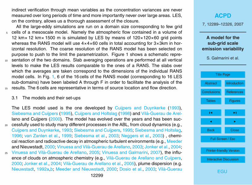
ABL reads (e.g., Stull, 1988; Garratt, 1994):

∂c′2

∂t+ uj

∂c′2

∂xj= −2u′

jc′

∂c

∂xj−

∂u′

jc′2

∂xj− 2ǫc, (1)

where from left to right the equation terms account for:

1. Time evolution of the concentration variance,15

2. Advection or transport term,

3. Production term due to turbulent motions within the mean concentration gradient,

4. Turbulent transport of variance,

5. Dissipation.

For the sake of simplicity we will consider here the one dimensional version of Eq. (1)20

in conditions of horizontal homogeneity, namely:

∂c′2

∂t= −2w ′c′

∂c

∂z−

∂w ′c′2

∂z− 2ǫc, (2)

12293




http://www.egu.eu

ACPD

7, 12289–12326, 2007

A model for the

sub-grid scale


S. Galmarini et al.

Title Page



Tables Figures

◭ ◮

◭ ◮

Back Close

Full Screen / Esc



EGU

all the consideration done hereafter can be extended to the remaining two spatial

dimensions. There are several conventional and well tested ways in which the unclosed

terms (3,4,5) of Eq. (2) can be parameterized. To avoid distracting the attention of our

readers from the actual central topic of this paper the parameterizations adopted are

presented in the Appendix.5

The concentration variance equation will be used as carrier of the information on the

emission heterogeneity from the surface to the upper atmospheric layers. We need

therefore to create a connection between the concentration variance equation and the

sub-grid emission. To do that we first express emissions in sub-grid terms. In general

let us assume Ei as the individual emission from a sub-grid scale surface within the10

grid-cell of a RANS model. Ei is defined as:

Ei =Mi

aiT,

where Mi is the amount of mass emitted per unit time T and ai is a sub-grid surface

that satisfies the condition:

ai<A,15

where A is the surface of the grid cell of the RANS model. The other conditions

on the sub-grid emitting surfaces is that given N the total number of sub-grid emitting

surfaces:

A =

N∑

i=1

ai .

At this point we will assume that we can decompose the emission into:20

Ei = E + E ′′

i, (3)

12294




http://www.egu.eu

ACPD

7, 12289–12326, 2007

A model for the

sub-grid scale


S. Galmarini et al.

Title Page



Tables Figures

◭ ◮

◭ ◮

Back Close

Full Screen / Esc



EGU

where:

E=1

A

N∑

i=1

aiEi . (4)

In the case in which the sub-grid scale emitting surfaces ai are of equal size (a) for all

i ’s (which is normally what is obtained as a result of the disaggregation of an emission

inventory at a scale smaller than the RANS model grid size) the average can also be5

calculated as:

E=1

Na

N∑

i=1

Mi

T. (5)

The different symbols used in Eq. (3) to identify average and fluctuation compared

to the notation of Eq. (1) and Eq. (2) are due to the fact that the average and conse-

quently the fluctuation should be considered over a surface whereas the overbar and10

the single accent are defined relative to a volume. We could at this stage imagine that

the emissions (average and fluctuation) pertain to a volume of air sitting right above

the surface. Eventually one could assume that the vertical extension of such volume

could go as far as the first numerical grid cell. As a matter of fact this is implicitly done

whenever a tracer is injected into a numerical model. Through this assumption we can15

now directly relate the two averaging operators (E and E ) so that the linearization of

the E now reads:

Ei=E + E ′

i, (6)

with Ei , E , and E ′

i now expressed as[mass L

−3T−1].

At this stage we will separate the contribution of the emission in the sense that the20

average emission (E ) will contribute to the average concentration (c) according to the

classical approach, while the emission fluctuation (E ′

i ) contributes to the concentration

12295




http://www.egu.eu

ACPD

7, 12289–12326, 2007

A model for the

sub-grid scale


S. Galmarini et al.

Title Page



Tables Figures

◭ ◮

◭ ◮

Back Close

Full Screen / Esc



EGU

fluctuation (c′). Therefore we re-derive the concentration variance equation taking into

account the emission fluctuation as an extra production term. Following the classic

derivation we first derive the conservation equation of the concentration fluctuation:

∂c′

∂t= w ′

∂c

∂z+

∂w ′c′

∂z+ E ′

+ νc∂2c′

∂2z, (7)

to which we have added the contribution of the emissions fluctuations. In the latter5

νc stands for molecular diffusion. Then we multiply both sides with 2c′and apply

derivation rules to obtain after averaging:

∂c′2

∂t= −2w ′c′

∂c

∂z+

∂w ′c′2

∂z+ 2c′E ′

− 2ǫc. (8)

The presence of the emission fluctuation has generated the extra term 2c′E ′ that we

will define concentration-emission covariance (CEC) term. The interesting aspect of10

Eq. (8) resides in the fact that we have added an extra term that represents a source of

variance and that is directly connected to the emission fluctuations. All the other terms

in the equation remain unchanged as one can see by comparing Eq. (8) with Eq. (2)

and therefore the parameterizations presented in Appendix are still valid. The new

variance equation accounts for a source term while the other terms create it, transport15

it, disperse it and dissipate it as expected from the turbulent motion thus acting as

carriers of the information to the upper layers.

The problem now is how to close the CEC term in order to make the equation solv-

able. If we start from the consideration that the correlation coefficient between the

concentration and the emission is formally given by:20

r =c′E ′

(E ′2)1/2 (

c′2)1/2

, (9)

12296




http://www.egu.eu

ACPD

7, 12289–12326, 2007

A model for the

sub-grid scale


S. Galmarini et al.

Title Page



Tables Figures

◭ ◮

◭ ◮

Back Close

Full Screen / Esc



EGU

we can derive a simple and straight forward parametrization of the CEC term as:

c′E ′ = r(E ′2)1/2 (

c′2)1/2

(10)

With expression Eq. (10) the closure has been transferred to the correlation coef-

ficient r which will be defined in the proceedings. The closure adopted has formally

restricted the range of variability of the closure constant r between 0 and 1 by defini-5

tion as negative values would be counter intuitive. In other words provided sufficient

level of turbulence intensity, close to the surface the concentration variance can only

be expected to increase with the increase of the emission fluctuation. In any case this

will be a hypothesis that needs to be verified and a more precise functional relationship

for r needs to be provided. Once r will be defined Eq. (7) will be closed. In fact the10

other term in Eq. (10), E ′2, can be calculated very simply from the emission inventory

as boundary condition of our problem. It will be the main character of this play and a

key parameter toward a better estimate of upper-air concentration levels. Following the

derivation of the average emission given by Eq. (4) the formula to calculate the volume

averaged emission variance in the case of generic sub-grid emitting surfaces ai reads:15

E ′2 = [1

A

N∑

i=1

ai (E − Ei )2]∆z,

where ∆z is the extension of the first grid point in the vertical. While for surfaces with

equal size it is:

E ′2 = [1

N

N∑

i=1

(E −

Mi

T)2]∆z.

12297




http://www.egu.eu

ACPD

7, 12289–12326, 2007

A model for the

sub-grid scale


S. Galmarini et al.

Title Page



Tables Figures

◭ ◮

◭ ◮

Back Close

Full Screen / Esc



EGU

It is worth to notice that the(E ′2)1/2

corresponds to the standard deviation of the

emission and represents the simplest way in which the sub-grid emission heterogene-

ity can be represented. It should be clear that the smaller the surfaces in which the

emission contributions are broken up below the RANS model grid size the higher the

variance and therefore the higher the detail in which the contribution will be accounted5

for. We have implicitly assumed that the emissions have a gaussian distribution around

the mean value which may sound as an over simplification but effectively it is a great

improvement with respect to the past.

To summarize the parameterization consists of calculating the sub-grid emission

variability from the emission inventory in terms of emission variance and to solve the10

concentration variance equation in which the extra contribution to the concentration

fluctuation has been included and closed as from Eq. (10). In this way going back

to a description provided above, the mean emission acts as source term of the mean

concentration and through Eq. (10) the emission variance effectively modulated by

the correlation coefficient acts as source term to the concentration variance equation.15

Average concentration emission and concentration standard deviation will be used si-

multaneously to describe the evolution of the tracer in the atmosphere.

3 Reynolds-averaged modeling vs Large eddy simulation

The way in which we are going to test the parametrization presented in the previous

section is by means of Large-Eddy Simulations (LES) of controlled emission cases20

and a three dimensional Reynolds Averaged Navier-Stokes (RANS) model. Large-

eddy simulation has been selected as it guarantees a detailed representation of the

turbulent flow and dispersion in the atmospheric boundary layer ranging from the peak

of maximum spectral energy down to the dissipation scale. In such controlled flow

conditions we are able to define specific, detailed and controlled emission scenarios.25

Any real case application selected to verify the parameterization will allow only an

12298




http://www.egu.eu

ACPD

7, 12289–12326, 2007

A model for the

sub-grid scale


S. Galmarini et al.

Title Page



Tables Figures

◭ ◮

◭ ◮

Back Close

Full Screen / Esc



EGU

indirect verification through mean variables as the concentration variances are never

measured over long periods of time and more importantly never over large areas. LES,

on the contrary, allows us a thorough assessment of the closure.

All the large-eddy simulations are run on a domain size corresponding to few grid

cells of a mesoscale model. Namely the atmospheric flow contained in a volume of5

12 km×12 km×1500 m is simulated by LES by means of 120×120×60 grid points

whereas the RANS model will use 4×4×60 cells in total accounting for 3×3km in hor-

izontal resolution. The coarse resolution of the RANS model has been selected on

purpose to push to the limit the parametrization. Figure 1 shows a schematic repre-

sentation of the two domains. Slab averaging operations are performed at all vertical10

levels to make the LES results comparable to the ones of a RANS. The slabs over

which the averages are taken correspond to the dimensions of the individual RANS

model cells. In Fig. 1, 6 of the 16 cells of the RANS model (corresponding to 16 LES

sub-domains) have been labeled A through F in order to facilitate the analysis of the

results. The 6 cells are representative in terms of source location and flow direction.15

3.1 The models and their set-ups

The LES model used is the one developed by Cuijpers and Duynkerke (1993),

Siebesma and Cuijpers (1995), Cuijpers and Holtslag (1998) and Vila-Guerau de Arel-

lano and Cuijpers (2000). The model has evolved over the years and has been suc-

cessfully used to study many different processes in the ABL, from cloud dynamics (e.g.,20

Cuijpers and Duynkerke, 1993; Siebesma and Cuijpers, 1995; Siebesma and Holtslag,

1996; van Zanten et al., 1999; Siebesma et al., 2003; Neggers et al., 2003) , chemi-

cal reaction and radioactive decay in atmospheric turbulent environments (e.g., Meeder

and Nieuwstadt, 2000; Vinuesa and Vila-Guerau de Arellano, 2003; Jonker et al., 2004;

Vinuesa and Vila-Guerau de Arellano, 2005; Vinuesa and Galmarini, 2007), the influ-25

ence of clouds on atmospheric chemistry (e.g., Vila-Guerau de Arellano and Cuijpers,

2000; Jonker et al., 2004; Vila-Guerau de Arellano et al., 2005), plume dispersion (e.g.

Nieuwstadt, 1992a,b; Meeder and Nieuwstadt, 2000; Dosio et al., 2003; Vila-Guerau

12299




http://www.egu.eu

ACPD

7, 12289–12326, 2007

A model for the

sub-grid scale


S. Galmarini et al.

Title Page



Tables Figures

◭ ◮

◭ ◮

Back Close

Full Screen / Esc



EGU

de Arellano et al., 2004; Dosio et al., 2005; Dosio and Vila-Guerau de Arellano, 2006),

stable BL (e.g., Galmarini et al., 1998; Beare et al., 2006). For a detailed description of

the model we refer the reader the above mentioned references.

A full RANS model has been selected for the sake of completeness of this study,

we could more simply have opted for a pure transport model and use the LES flow5

to run the dispersion. The three-dimensional RANS model is the mesoscale model

described in detail by Martilli (2002). The concentration mean equation for the transport

of a passive scalar together with the full three-dimensional formulation of the variance

Eq. (8) have been added to the original model formulation for the sake of this study.

The LES simulation runs for 3 h with maximum time-step used in the calculations is10

0.5s−1

. The surface sensible heat flux is set at 0.05 Km s−1

. A constant westerly wind of

5ms−1

has been imposed. The initial potential temperature profile has a constant value

of 288K below 662.5m and increases by 6K above 712.5m. The surface roughness

length z0 is set to 0.01m. Periodic lateral boundary conditions are assumed. At the

end of the first hour temperature and wind profile are provide to the RANS models as15

initial condition for its simulation. LES data are averaged over the last simulation hour

before they are compared with the RANS results.

3.2 Flow and turbulence simulations

Before we analyze the tracer release set up and the results relating to the scalar vari-

ance we present here the results of the flow simulation comparison of RANS vs LES.20

Figures 2a-d show the vertical profile of M (total wind) and potential temperature Θ,

turbulent kinetic energy and heat flux respectively calculated by the LES and RANS

for sub-domain. The plots relate to sub-grid cell C only (see Fig. 1) as the same re-

sult is obtained in the others. The RANS model is able to simulate with a relatively

high degree of accuracy the wind speed and direction simulated by the LES. Small25

discrepancies are found for M that shows a slight systematic underestimation of the

LES profile. On the temperature the agreement with the LES is very good in spite of a

slightly higher diffusivity of the RANS model at the boundary layer top that lead to a dif-

12300




http://www.egu.eu

ACPD

7, 12289–12326, 2007

A model for the

sub-grid scale


S. Galmarini et al.

Title Page



Tables Figures

◭ ◮

◭ ◮

Back Close

Full Screen / Esc



EGU

ferent slope in the temperature profile and the inversion. The turbulence intensity and

distribution is presented in Fig. 2c by the profile of the turbulent kinetic energy. Even for

this variable the comparison between the two models can be considered satisfactory

in spite of differences of curvature in the vertical profile and an underestimation at the

boundary layer top. The heat flux is modeled very well by the RANS model including5

the negative flux component at the boundary layer top.

4 Sub-grid scale emission: evaluation of the parametrization

The simplest way to create a sub-grid scale emission heterogeneity is to consider a

single area source emitting within one of the RANS cells that varies in size from total

coverage of the cell to the minimum resolvable size for the LES. Three different emis-10

sion scenarios were simulated. For the first the passive tracer is released over the

entire RANS grid element (see Fig. 1). The remaining three cover the grid elements

corresponding to 64, 44 and 28% of the grid surface thus leading to an increasing sub-

grid scale variability of the emission and corresponding emission variance. The tracer

released has initially zero concentration. Each emitting surface releases continuously15

with an emission rate of 0.1 ppbs−1

. The flux is maintained constant in spite of the

change in the size of the emitting surface. Non-periodic boundary conditions are used

for the tracer. The simulations run for 3 h for the dynamic and 2 h for the tracer disper-

sion. In the LES non-periodic boundary conditions are set up for the scalars. All the

results relate to the last hour of the simulation. Figures 3a through c represent snap20

shots of the evolution of the dispersion process as simulated by the LES. Figures 3a

shows a top view of the largest emission pattern (blue contour) and the smallest (ma-

genta contour) after 5 min from the release start. The figure shows also the RANS grid

(in red) and for one RANS grid cell the LES grid (in black). From the figure one can

appreciate the difference in size between the two scenarios, the scales involved in the25

dispersion process, and the scales falling into a RANS grid that would not be resolved

by the RANS model. Figures 3b and c show to subsequent stages of evolution of the

12301




http://www.egu.eu

ACPD

7, 12289–12326, 2007

A model for the

sub-grid scale


S. Galmarini et al.

Title Page



Tables Figures

◭ ◮

◭ ◮

Back Close

Full Screen / Esc



EGU

emissions at 10 and 25 min from release start. The contours on the bottom of the sim-

ulation domain relate to surface temperature while on the domain walls they relate to

vertical velocity.

Figures 4a show the mean concentration profiles calculated in the six RANS cells

(6 LES sub domains). The results of RANS (dashed line) remain the same in spite5

of the variability of the emitting scenario since the average emission rate remains un-

changed. The LES results (continuous line) vary from one case to the other. Most

of the mass is concentrated in the emitting cell (cell C) and is advected eastward. A

small amount of mass is predicted in cells A and B by the RANS model due to the

small discrepancies in the wind field prediction. The average concentration behavior10

can also be considered comparable among the two models having considered the fact

the RANS model at this level does not take into account the sub-grid scale variability

of the emission intensity. This is as far as any mesoscale transport model can get:

modeling the mean concentration evolution from the mean emission rate. The discrep-

ancies in predicting the mean concentration are largely due to the coarse resolution of15

the RANS model. Figures 4b show the same calculation performed for Figs. 4a but with

a 1 km×1 km grid resolution. The results improve systematically. The reason for the

selection of the coarse resolution of 3×3 km2

is twofold. As anticipated earlier, first we

wanted to test the parametrization on a mesoscale average grid size secondly 1×1 km2

would have reduced the surface emission size to the extent that also in the LES only20

few cells would have been available to simulate the release thus reducing the accuracy

of the calculation.

Let us now consider the new parametrization to account for the emission hetero-

geneity within the RANS model. In order to implement our parametrization in the RANS

model we still have the unsolved problem of the closure of the emission-concentration25

correlation coefficient introduced in Sect. 2. We will make use here of the high reso-

lution simulations to study the correlation coefficient behavior and try to find a simple

functional relationship to assign it a value. Figure 5 shows the variation of the cor-

relation coefficient between the emission and the concentration calculated explicitly

12302




http://www.egu.eu

ACPD

7, 12289–12326, 2007

A model for the

sub-grid scale


S. Galmarini et al.

Title Page



Tables Figures

◭ ◮

◭ ◮

Back Close

Full Screen / Esc



EGU

from the LES model as a function of the horizontal dimension of the emitting surface.

Not unexpectedly the coefficient tends to zero as the surface shrinks and to one as it

widens. the correlation coefficient has been calculate also for other surface sizes than

the four analysed here. Although the trend appears to be linear it is expected to flatten

toward 1 in a sort of square-root trend. Figure 6 shows the variability of the correlation5

coefficient as a function of height assuming therefore that the first computational grid

point sits at 12.5 m (squares), 37.5 m (triangle), 62.5 m (diamond), 87.5 m (star) and

112.5 m (cross). As it can be seen in all cases the correlation coefficient shows a well

behaved trend that can easily be framed in a functional relationship. However we will

not do this in this study as we realise that a dedicated research will need to be per-10

formed on the subject toward the definition of a general formulation. For the sake of

this study we will use the coefficient values extracted from the plot of Fig. 5 as we still

want to prove that the parameterization is valid. A sensitivity analysis on the impact

of an approximated value on the performance of the parametrization will need to be

performed as well as its dependence on wind speed, heat flux and height.15

Having identified a correlation coefficient we can close our parametrization and

calculate the concentration variance produced by the emission variability. Fig-

ures 7, 8 and 9 show the vertical profile of concentration variance calculated by the

RANS model and the LES (continuous line) for the 64, 44, 28% values of emission

variance respectively. The parametrization seems to work extremely well in the emis-20

sion cell where most of the variance is produced in correspondence with the largest

concentration gradients. This is valid also for the other two cases with a slight over-

estimation of the values through out the profile. In all three cases in cell D the values

in the bulk of the boundary layer are very well reproduced, while a large discrepancy

is present close to the surface that can be attributed to an excess in dissipation of the25

RANS formulation. The differences are more marked as the emitting surface shrinks.

In cells A and B for all the three cases we notice an over prediction by the RANS model

that can be connected to the fact that the latter predicts a non zero concentration in

those two cells as described earlier. In all the cases we notice that the discrepancies

12303




http://www.egu.eu

ACPD

7, 12289–12326, 2007

A model for the

sub-grid scale


S. Galmarini et al.

Title Page



Tables Figures

◭ ◮

◭ ◮

Back Close

Full Screen / Esc



EGU

are there but pertain to values of concentration variance that is one order of magnitude

smaller than in the emitting cell. It is in fact interesting to notice that the dissipation of

concentration variance takes place over a relatively short time scale thus not permitting

its advection to the neighboring cells as also confirmed by the LES results. In the ver-

tical its values are relevant in the first half of the boundary layer and decrease rapidly5

from there to the its top.

A direct evidence of the impact of emission heterogeneity to upper air concentration

can be obtained by sampling the LES domain at specific points in time. We will call

these point virtual monitoring stations since they will behave like sampling stations in

the real atmosphere which can have only a partial view of the process but can describe10

it in great detail in time. Figures 10 shows the location of the station (a) and two time

series (b and c) for the 64% percent emission surface (depicted in (a) as instantaneous

concentration contour) and station (d) and the corresponding time series for the 24%

emission (e and f). Figures 10b and e refer to the comparison of the one minute av-

eraged concentration time series from the LES (red curve) and RANS (black curve).15

Figures 10c and f shows the comparison of the 5 min average concentration time se-

ries from the two models. In both figures the shaded area covers the c ± c′2 where

the standard deviation is the result of the parametrization within the RANS model. The

results show a remarkable correspondence between the RANS average concentration

plus the standard deviation and the LES time series for both cases. A slight underesti-20

mation of the LES results is shown by the RANS mean concentration but all fluctuations

fall well within the standard deviation. The same is true for the other station selected for

the emission domain and shown in Figs. 11a–f . In particular in the latter we see that

most of the deviation is due to the lack of agreement in the average concentration but

that the bandwidth of the standard deviation covers all the RANS-sub-grid fluctuations25

explicitly calculated by the LES. Moving to the grid-cells downwind (Figs. 12–14 (a–f))

of the emission we notice, that still the variance has a relevant role in catching the

sub-grid fluctuation. One can also notice the variability of the variance by comparing

the large surface emission with the smallest. In all three virtual monitoring stations the

12304




http://www.egu.eu

ACPD

7, 12289–12326, 2007

A model for the

sub-grid scale


S. Galmarini et al.

Title Page



Tables Figures

◭ ◮

◭ ◮

Back Close

Full Screen / Esc



EGU

mesoscale model is not able to catch the quasi-instantaneous results of the LES which

is very dependent on where the cloud shows up with respect to the station (see Fig. 3

for example) but when the data are time averaged to longer time scales, the RANS

variance and its use is making the difference in for the interpretation of the results. It

should be underlined that the case simulated is extremely complicated for any RANS5

model especially at these resolutions. One should not forget that the ratio of resolu-

tion of the two models is 960/864000 and disregarding the fact that the two models

have the same vertical resolution the RANS with the new parametrization models with

16 grid cells what the LES models with 14 400.

5 Conclusions10

A method to account for the sub-grid emission heterogeneity has been proposed. The

method is based on the modification of the concentration variance equation and the

assumption that emission can be linearized in an average and a fluctuating part and

a correlation between emission and air concentration within the model grid cell. The

ingredients for the application of the parametrization is the availability of an emission15

inventory that can provide disaggregated values at a scale smaller that the grid used in

the transport model. The method allows one to explicitly calculate the time evolution of

the concentration variance in every grid cell, its transport and dissipation as well as the

contribution of the emission variability at the surface to its creation. The parametrization

presented in this paper can be applied to any model from meso- to global scale. In fact20

the assumption normally made in these two kind of models with respect to emission

treatment are the same. For the first time, the method proposed allows to calculate

explicitly the time evolution of the sub-grid variability of a variable and to attach it to the

mean concentration value. The parametrization has been made part of a mesoscale

model and the results on a variety of cases compared with high resolution simulation25

performed with a Large Eddy Simulation model. The results show a very satisfactory

agreement.

12305




http://www.egu.eu

ACPD

7, 12289–12326, 2007

A model for the

sub-grid scale


S. Galmarini et al.

Title Page



Tables Figures

◭ ◮

◭ ◮

Back Close

Full Screen / Esc



EGU

More generically the concept developed here could be applied in several other con-

texts like:

1. Homogeneous emission of inert or reacting scalars. In this case the new term

of the concentration variance equation would vanish but still there would be an

impact of the concentration variance equation which has never been accounted5

for. The concentration variance is a statistical representation of the effect of inho-

mogeneous turbulent mixing. Therefore regardless of the modification introduced

in this paper to the variance equation, it could be used to account for the sub-

grid mixing. To date, no mesoscale model has taken explicitly into account this

element. Indeed the effect is relevant within the boundary layer, which is a small10

portion of the atmosphere represented by a global model for example, but yet

there is where the comparison with surface measurements takes place.

2. The method proposed here could be applied to inert scalars in-homogeneously

emitted at the surface like for example heat or moisture emitted from the surface.

An element of concern could be the fact that every species will require an additional15

equation to be solved and that it may constitute a burden for large chemical scheme,

however we could consider to use it only to primary pollutants. Furthermore the solu-

tion of the highly parameterized variance equation is straight forward and inexpensive.

Another concern may relate to the effect of chemical reaction on the new variable. In

other words would the scalar react should we take into account the chemical reaction20

also at the level of the concentration variance? An answer to this problem has already

been given by the large number of studies performed since the 1990s on the influence

of turbulent mixing on chemical reaction in the atmosphere (e.g., Sykes et al., 1994;

Galmarini et al., 1997; Verver et al., 1997; Vinuesa and Vila-Guerau de Arellano, 2003,

2005). These works have shown that the discrimination in the application of chemical25

reaction to the second order model equation is the ratio of the time scale of turbu-

lence and that of chemistry. A finite number of species in the atmosphere fulfill this

requirement and only for those chemistry should be take into account.

12306




http://www.egu.eu

ACPD

7, 12289–12326, 2007

A model for the

sub-grid scale


S. Galmarini et al.

Title Page



Tables Figures

◭ ◮

◭ ◮

Back Close

Full Screen / Esc



EGU

The next steps of our research will concentrate on the following aspects:

1. frame in the most general way the correlation coefficient between emission and

concentration in air,

2. verify the sensitivity of the parametrization on the vertical resolution of the

mesoscale model,5

3. apply the mesoscale model to a real case study,

4. develop a parametrization to account for the sub-grid topological orientation of the

emission heterogeneity.

In this last case the only possibility to test the parametrization will be by comparison

of the predicted concentration plus and minus the variance and the measured ones, so10

only indirectly. Therefore the case will be selected to as dominated by large emission

variability.

Acknowledgements. All computations were performed on the Linux cluster of the PROCAS

action of the Institute for Environment and Sustainability. The authors wish to thank A. Stips

and P. Simons who kindly provided the access to this facility.15

Appendix A

Closures used for prognostic equation of the variance of pollutant

concentration

A description of the other closures used to solve the prognostic equation for the vari-20

ance Eq. (8) is given.

The turbulent fluxes of (1) are calculated as

w ′c′ = −

Kz

P r

∂c

∂z(A1)

12307




http://www.egu.eu

ACPD

7, 12289–12326, 2007

A model for the

sub-grid scale


S. Galmarini et al.

Title Page



Tables Figures

◭ ◮

◭ ◮

Back Close

Full Screen / Esc



EGU

where the turbulent coefficient Kz is estimated using a K-l closure (Bougeault and

Lacarrere, 1989). In this closure a prognostic equation for the turbulent kinetic energy

e is solved, and turbulent coefficients and TKE dissipation are derived using length

scales as follows:

Kz=Ck lke1/2 (A2)5

ǫe=Cǫ

e3/2

lǫ(A3)

The lengths lk and lǫ are calculated at a particular level from the possible upward and

downward displacements (lup and ldown) that air parcels with kinetic energy e originating

from the level z could accomplish before being stopped by buoyancy.

∫ z+lup

zβ (θ(z) − θ(z′))dz′=e(z), (A4)10

∫ z

z−ldown

β (θ(z′) − θ(z))dz′ = e(z), (A5)

(A6)

(Therry and Lacarrere, 1983) proposed a relationship between lǫ and lk :

lk =

(1 +

g

θ

wθlǫ

Cǫe3/2

lǫ

)lǫ (A7)

(Belair et al., 1999) used the budget equation for the TKE to derive the relationship15

neglecting the turbulent transport contribution and assuming steady-state. This leads

to

lk =

(1 +

Be

De

)lǫ (A8)

12308




http://www.egu.eu

ACPD

7, 12289–12326, 2007

A model for the

sub-grid scale


S. Galmarini et al.

Title Page



Tables Figures

◭ ◮

◭ ◮

Back Close

Full Screen / Esc



EGU

or

lk =

(2Be + Ge

Be + Ge

)lǫ (A9)

where Be, De and Ge are the buoyancy, the dissipation and the gradient terms of

the TKE budget equation. lk is determined as the minimum between lup and ldown

(Bougeault and Lacarrere, 1989).5

The turbulent transport of variance can be written as

∂ujc′2

∂xj= −

∂

∂z

(Kz

P r

∂c′2

∂z

)(A10)

The dissipation can be written as

2ǫc′2

=c′2

τc′2

(A11)

(Verver et al., 1997) used the TKE dissipation timescale divided by 2.5 as variance10

dissipation timescale to be inserted in the expression of the scalar variance dissipation.

Using this expression together with (A3) leads to

ǫc′2

= 2.5Cǫ

e1/2

lǫc′2 (A12)

Cǫ and Ck are set to 0.125 and 0.7 and the Prandtl P r number is 1/1.3. Boundary

conditions for the TKE and the variances are calculated assuming no gradients across15

the surface.

12309




http://www.egu.eu

ACPD

7, 12289–12326, 2007

A model for the

sub-grid scale


S. Galmarini et al.

Title Page



Tables Figures

◭ ◮

◭ ◮

Back Close

Full Screen / Esc



EGU

References

Belair, S., Mailhot, J., Strapp, J. W. and MacPherson, J. I.: An examination of local versus

nonlocal aspects of a TKE-based boundary-layer scheme in clear convective conditions, J.

Appl. Meteorol., 38, 1499–1518, 1999. 12308

Beare, R. J., Macvean, M. K., Holtslag, A. A. M., Cuxart, J., Esau, I., Golaz, J.-C., Jimenez,5

M. A., Khairoutdinov, M., Kosovic, B, Lewellen, D., Lund, T. S., Lundquist, J. K., Mccabe,

A., Moene, A. F., Noh, Y., Raasch, S., and Sullivan P.: An intercomparison of large-eddy

simulations of the stable boundary layer, Boundary-Layer Meteorol., 118, 247–272, 2006.

12300

Bougeault, P., and Lacarrere, P.: Parameterization of orography-induced turbulence in a10

mesobeta-scale model, Mon. Weather Rev., 117, 1872–1890, 1989. 12308, 12309

Cuijpers, J. W. M., and Duynkerke P. G.: Large eddy simulations of trade wind with cumulus

clouds, J. Atmos. Sci. 50, 3894–3908, 1993. 12299

Cuijpers, J. W. M., and Holtslag A. A. M.: Impact of skewness and nonlocal effects on scalar

and buoyancy fluxes in convective boundary layers, J. Atmos. Sci. 55, 151–162, 1998. 1229915

Dosio, A., Vila-Guerau de Arellano, J., Holtslag, A. A. M., and Builtjes P. J. H.: Dispersion

of a passive tracer in buoyancy- and shear-driven boundary layers, J. Appl. Meteorol., 42,

1116—1130, 2003. 12299

Dosio, A., Vila-Guerau de Arellano, J., Holtslag, A. A. M., and Builtjes P. J. H.: Relating eulerian

and lagrangian statistics for the turbulent dispersion in the atmospheric convective boundary20

layer, J. Atmos. Sci., 62, 1175–1191, 2005. 12300

Dosio, A., and Vila-Guerau de Arellano J.: Statistics of absolute and relative dispersion in the

atmospheric convective boundary layer: a large-eddy simulation study, J. Atmos. Sci., 63,

1253–1272, 2006. 12300

Galmarini, S., Vila-Guerau de Arellano, J. and Duynkerke P. G.: Scaling the turbulent transport25

of chemical compounds in the surface layer under neutral and stratified conditions. Q. J. R.

Meteorol. Soc., 123, pp. 223–242, 1997. 12306

Galmarini, S., Beets K., and Duynkerke, P. G.: Stable nocturnal boundary layers: a comparison

of one-dimensional and large-eddy simulation models. Bound.-Lay. Meteorol., 88, 181–210,

1998. 1230030

Garratt, J. R.: The atmospheric boundary layer. Cambridge university press, 316 pp., 1994.

12293

12310




http://www.egu.eu

ACPD

7, 12289–12326, 2007

A model for the

sub-grid scale


S. Galmarini et al.

Title Page



Tables Figures

◭ ◮

◭ ◮

Back Close

Full Screen / Esc



EGU

Jonker, H. J. J., Vila-Guerau de Arellano, J. and Duynkerke P. G.: Characteristic length scales

of reactive species in a convective boundary layer, J. Atmos. Sci., 61, 41–56, 2004. 12299

Martilli, A.: Numerical study of urban impact on boundary layer structure: sensitivity to wind

speed, urban morphology, and rural soil moisture, J. Appl. Meteorol., 41, 1247–1266, 2002.

123005

Meeder, J. P. and Nieuwstadt, F. T. M.: Large-eddy simulation of the turbulent dispersion of

a reactive plume from a point source into a neutral atmospheric boundary layer, Atmos.

Environ., 34, 3563–3573, 2000. 12299

Molemaker, M. J., Vila-Guerau de Arellano, J.: Turbulent control of chemical reactions in the

convective boundary layer, J. Atmos. Sci., 55, 568–579, 1998.10

Neggers, R. A. J., Jonker, H. J. J., and Siebesma A.P.: Size statistics of cumulus cloud popula-

tions in large-eddy simulations, J. Atmos. Sci., 60, 1060—1074, 2003. 12299

Nieuwstadt, F.T.M.: A large-eddy simulation of a line source in a convective atmospheric bound-

ary layer—I, dispersion characteristics, Atmos. Environ., 26A, 485–495, 1992a. 12299

Nieuwstadt, F. T. M.: A large-eddy simulation of a linesource in a convective atmospheric15

boundary layer—II, dynamics of a buoyant line source, Atmos. Environ., 26A, 497–503,

1992b. 12299

Siebesma, A. P., and Cuijpers J. W. M.: Evaluation of parametric assumptions for shallow

cumulus convection, J. Atmos. Sci. 52, 650–666, 1995. 12299

Siebesma, A. P., and Holtslag, A. A. M.: Model impacts of entrainment and detrainment rates20

in shallow cumulus convection, J. Atmos. Sci., 53 2354–2364, 1996. 12299

Siebesma, A. P., Bretherton, C. S., Brown, A., Chlond, A., Cuxart, J., Duynkerke, P. G., Jiang,

H., Khairoutdinov, M., Lewellen, D., Moeng, C. H., Sanchez, E., Stevens, B., and Stevens D.

E.: A large eddy simulation intercomparison study of shallow cumulus convection, J. Atmos.

Sci., 60, 1201–1219, 2003. 1229925

Stull, R. B.: An introduction to boundary-layer meteorology. Kluwer academic publishers, 670

pp, 1988. 12293

Sykes, R. I., Parker, S. F., Henn, D. S., Lewellen, W. S.: Turbulent mixing with chemical reactions

in the planetary boundary layer, J. Appl. Meteorol., 33, 825–834, 1994. 12306

Therry, G., and Lacarrere, P.: Improving the eddy kinetic energy model for planetary boundary30

layer description, Bound.-Lay. Meteorol., 25, 63–88, 1983. 12308

van Zanten, M., Duynkerke, P. G., and Cuijpers J. W. M.: Entrainment parameterizations in

convective boundary layers, J. Atmos. Sci. 56, 813—828, 1999. 12299

12311




http://www.egu.eu

ACPD

7, 12289–12326, 2007

A model for the

sub-grid scale


S. Galmarini et al.

Title Page



Tables Figures

◭ ◮

◭ ◮

Back Close

Full Screen / Esc



EGU

Verver, G. H. L, Van Dop, H. and Holtslag, A. A. M.: Turbulent mixing of reactive gases in the

convective boundary layer, Bound.-Lay. Meteorol., 85, 197–222, 1997. 12306, 12309

Vila -Guerau de Arellano, J., and Cuijpers J. W. M.: The chemistry of a dry cloud: the effects of

radiation and turbulence, J. Atmos. Sci. 57, 1573–1584, 2000. 12299

Vila-Guerau de Arellano, J., Dosio, A., Vinuesa, J.-F., Holtslag, A. A. M, and Galmarini, S.: The5

dispersion of chemically reactive species in the convective boundary layer, Meteorol. Atmos.

Phys., 87, 23–28, 2004. 12299

Vila-Guerau de Arellano, J., Kim, S.-W., Barth, M. C., and Patton, E. G.: Transport and chemical

transformations influenced by shallow cumulus over land, Atmos. Chem. Phys., 5, 3219–

3231, 2005 1229910

Vinuesa, J.-F. and Vila -Guerau de Arellano, J.: Fluxes and (co-)variances of reacting scalars

in the convective boundary layer, Tellus 55B, 935—949, 2003. 12299, 12306

Vinuesa, J.-F. and Vila -Guerau de Arellano, J.: Introducing effective reaction rates to account

for the inefficient mixing of the convective boundary layer, Atmos. Environ., 39, 445–461,

2005. 12299, 1230615

Vinuesa, J.-F. and Galmarini, S.: Characterization of the222

Rn family turbulent transport in the

convective atmospheric boundary layer, Atmos. Chem. Phys., 7, 697–712, 2007,

http://www.atmos-chem-phys.net/7/697/2007/. 12299

12312




http://www.egu.eu

http://www.atmos-chem-phys.net/7/697/2007/

ACPD

7, 12289–12326, 2007

A model for the

sub-grid scale


S. Galmarini et al.

Title Page



Tables Figures

◭ ◮

◭ ◮

Back Close

Full Screen / Esc



EGU

Fig. 1. Schematic representation of the the two model computational grids and emission

scenarios. Left panel: RANS grid. Letters A to F identify grid where results will be shown.

Cell C contains the various emission patterns ranging fro 100% coverge of the grid to 28%

coverage. Righ panel LES grid. In red the sub-domains corresponding to the RANS grid over

which the LES results are averaged.

12313




http://www.egu.eu

ACPD

7, 12289–12326, 2007

A model for the

sub-grid scale


S. Galmarini et al.

Title Page



Tables Figures

◭ ◮

◭ ◮

Back Close

Full Screen / Esc



EGU

(a) (b)

(c) (d)

Fig. 2. Comparison of RANS (dashed line) and LES (continuous line) dynamical variables. (a)

total wind speed, (b) potential temperature, (c) Turbulent kinetic energy, (d) turbulent heat flux.

12314




http://www.egu.eu

ACPD

7, 12289–12326, 2007

A model for the

sub-grid scale


S. Galmarini et al.

Title Page



Tables Figures

◭ ◮

◭ ◮

Back Close

Full Screen / Esc



EGU

(a) (b)

(c)

Fig. 3. Snapshots of the tracer dispersion (5 min after the release start) as from the Large-Eddy

simulation. (a) top view of the releases from the two surfaces namely 100% of the RANS grid

cell (blue), 24% of the RANS grid cell (purple). In (a) the grid corresponds to the RANS grid

and the LES sub-domains over which LES results have been averaged. In the lowest left corner

a sample of the actual LES grid. (b) and (c) two different stages of the tracers dispersion at

10 min and 25 min respectively after the release start. Colors on the bottom layers correspond

to turbulent heat flux and on vertical wall to vertical velocity.

12315




http://www.egu.eu

ACPD

7, 12289–12326, 2007

A model for the

sub-grid scale


S. Galmarini et al.

Title Page



Tables Figures

◭ ◮

◭ ◮

Back Close

Full Screen / Esc



EGU

(a) (b)

Fig. 4. (a) Vertical profiles of the tracers mean concentration in the 6 grid cells labeled a through

f and depicted in Fig. 1. The vertical coordinate is normalized by the boundary layer height.

Continuous line LES results, dashed line RANS model. The results relate to the 3×3 km RANS

model resolution. (b) same as (a) but with RANS model running at 1×1 km resolution.

12316




http://www.egu.eu

ACPD

7, 12289–12326, 2007

A model for the

sub-grid scale


S. Galmarini et al.

Title Page



Tables Figures

◭ ◮

◭ ◮

Back Close

Full Screen / Esc



EGU

Fig. 5. Correlation coefficient of concentration and emission as a function of the horizontal

extension of the emitting surface.

12317




http://www.egu.eu

ACPD

7, 12289–12326, 2007

A model for the

sub-grid scale


S. Galmarini et al.

Title Page



Tables Figures

◭ ◮

◭ ◮

Back Close

Full Screen / Esc



EGU

Fig. 6. Same as Fig. 5. The different simples give the dependence of the correlation coefficient

on height. Squares 12.5 m from the surface, triangles 37.5 m, diamond 62.5 m, star 87.5 m,

cross 112.5 m.

12318




http://www.egu.eu

ACPD

7, 12289–12326, 2007

A model for the

sub-grid scale


S. Galmarini et al.

Title Page



Tables Figures

◭ ◮

◭ ◮

Back Close

Full Screen / Esc



EGU

Fig. 7. Comparison of the vertical profile of concentration variance calculated by the RANS

(dashed line) and LES (continuous line) models. The vertical coordinate is normalized by the

boundary layer height. The results relate to the RANS model grid cell and corresponding LES

sub-domains depicted in Fig. 1. The results relate to the emission surface of 64% of the RANS

grid size.12319




http://www.egu.eu

ACPD

7, 12289–12326, 2007

A model for the

sub-grid scale


S. Galmarini et al.

Title Page



Tables Figures

◭ ◮

◭ ◮

Back Close

Full Screen / Esc



EGU

Fig. 8. Same as Fig. 7. The results relate to the emission surface of 44% of the RANS grid

size.

12320




http://www.egu.eu

ACPD

7, 12289–12326, 2007

A model for the

sub-grid scale


S. Galmarini et al.

Title Page



Tables Figures

◭ ◮

◭ ◮

Back Close

Full Screen / Esc



EGU

Fig. 9. Same as Fig. 7. The results relate to the emission surface of 28% of the RANS grid

size.

12321




http://www.egu.eu

ACPD

7, 12289–12326, 2007

A model for the

sub-grid scale


S. Galmarini et al.

Title Page



Tables Figures

◭ ◮

◭ ◮

Back Close

Full Screen / Esc



EGU

(a) (d)

(b) (e)

(c) (f)

Fig. 10. (a and d) Emission scenarios and position of the virtual station with respect to the

RANS grid. (a) 64% surface emission, (d) 28% surface emission. (b and e) comparison of

the time evolution of the RANS concentration (continuous line) plus and minus standard devi-

ation (hatched surface) with the concentration from the LES (red line) both model results are

averaged in time over 1 min. (c and f) same as (b and e) but with model results averaged over

5 min.12322




http://www.egu.eu

ACPD

7, 12289–12326, 2007

A model for the

sub-grid scale


S. Galmarini et al.

Title Page



Tables Figures

◭ ◮

◭ ◮

Back Close

Full Screen / Esc



EGU

(a) (d)

(b) (e)

(c) (f)

Fig. 11. Same as Fig. 10 but different sampling virtual station.

12323




http://www.egu.eu

ACPD

7, 12289–12326, 2007

A model for the

sub-grid scale


S. Galmarini et al.

Title Page



Tables Figures

◭ ◮

◭ ◮

Back Close

Full Screen / Esc



EGU

(a) (d)

(b) (e)

(c) (f)


12324




http://www.egu.eu

ACPD

7, 12289–12326, 2007

A model for the

sub-grid scale


S. Galmarini et al.

Title Page



Tables Figures

◭ ◮

◭ ◮

Back Close

Full Screen / Esc



EGU

(a) (d)

(b) (e)

(c) (f)


12325




http://www.egu.eu

ACPD

7, 12289–12326, 2007

A model for the

sub-grid scale


S. Galmarini et al.

Title Page



Tables Figures

◭ ◮

◭ ◮

Back Close

Full Screen / Esc



EGU

(a) (d)

(b) (e)

(c) (f)


12326




http://www.egu.eu

Modelling the impact of sub-grid scale emission ...

Documents

Transcript of Modelling the impact of sub-grid scale emission ...