Modelling the dissociation dynamics and threshold...

MODELLING THE

DISSOCIATION DYNAMICS

AND THRESHOLD PHOTOELECTRON

SPECTRA OF SMALL HALOGENATED

MOLECULES

by

Jonelle Harvey

A thesis submitted to

The University of Birmingham

for the degree of

DOCTOR OF PHILOSOPHY

School of Chemistry

University of Birmingham

March 2013

University of Birmingham Research Archive

e-theses repository This unpublished thesis/dissertation is copyright of the author and/or third parties. The intellectual property rights of the author or third parties in respect of this work are as defined by The Copyright Designs and Patents Act 1988 or as modified by any successor legislation. Any use made of information contained in this thesis/dissertation must be in accordance with that legislation and must be properly acknowledged. Further distribution or reproduction in any format is prohibited without the permission of the copyright holder.

Abstract The two experimental aspects of the imagining photoelectron

photoion coincidence (iPEPICO) apparatus which is stationed at the

VUV Beamline at the Swiss Light Source, a synchrotron source, have

been used to investigate the fundamental properties of small

molecules in the gas phase.

The fast and slow dissociation dynamics of halogenated

methanes and fluorinated ethenes have been investigated using

threshold photoelectron photoion coincidence (TPEPICO) techniques.

Rate constants and accurate 0 K appearance energies for the

formation of subsequent daughter ions have been determined. The

latter values have been used in conjunction with ab initio calculations

to derive updated enthalpies of formation.

The valence threshold photoelectron spectra of four

fluorinated ethenes have been recorded. The spectra have been

analysed using Franck–Condon simulations to model the vibrational

structure, and assign the spectra, sometimes revising previous

assignments. The potential energy surfaces of the ground and excited

electronic states have been explored to uncover their various

intriguing dissociative photodissociation mechanisms.

With thanks to John Harvey, George Anderson

Andras Bodi, Michael Parkes, Nicola Rogers and Richard Tuckett

Deity of Science

Acrylic on canvas, dimensions 80 × 60 cm

Award winning original art work by the author depicting

the iPEPICO endstation and the constant stream of

information from reactions generated from within.

Publications

J. Harvey, R. P. Tuckett and A. Bodi, ‘A Halomethane Thermochemical Network from iPEPICO Experiments and Quantum Chemical Calculations’., Journal of Physical Chemistry A, (2012), volume 116, issue 39, pages 9696-9705.

J. Harvey, A. Bodi, R. P. Tuckett and B. Sztáray, ‘Dissociation dynamics of fluorinated ethene cations: from time bombs on a molecular level to double-regime dissociators’., Physical Chemistry Chemical Physics, (2012), volume 14, pages 3935-3948.

J. Harvey, Patrick Hemberger, A. Bodi and R. P. Tuckett, ‘Vibrational and electronic excitations in fluorinated ethene cations from the ground up’, Journal of Chemical Physics, (2013), volume 138, pages 124301-124313.

Contents

Chapter 1: Introduction 1

1.A. Measuring the photoelectron signal

3

1.A.1. Photoelectron Spectroscopy (PES)

3

1.A.2. Threshold Photoelectron Spectroscopy (TPES)

5

1.A.3. Ionization energies 8

1.A.4. What determines the observed spectra?

10

1.A.5. Potential energy surfaces 13

1.B. The study of ionic dissociations 16

1.B.1.Threshold Photoelectron Photoion Coincidence (TPEPICO)

21

1.B.2.Modelling the results of TPEPICO experiments

23

1.B.3. Unimolecular rate theories 25

1.B.3.1.Rice–Ramsperger–Kassel–Marcus (RRKM) theory

26

1.B.4. Kinetic and competitive shifts 34

1.C. Thermochemistry 35

1.C.1 Thermochemical values derived from iPEPICO

35

1.C.2 Isodesmic reactions 38

References 40

Chapter 2: Experimental 43

2.A. The synchrotron radiation source

44

2.B. The endstation 49 2.C. Capturing the electron signal 51

2.D. The experimental results 55

References 56

Chapter 3: Theory 58

3.A. Computational methods 59

3.A.1. Calculating molecular geometries and potential energy paths

59

3.A.2. Composite methods 61

3.B. Modelling 67

3.B.1. Modelling the breakdown curves 67

3.B.1.1. Fast dissociations 68

3.B.1.2. Slow dissociations 71

2.B.1.3. Parallel and consecutive reactions

74

2.B.2. Modelling the TPES 76

References 80

Chapter 4: Fast dissociations of halogenated methanes: a thermochemical network.

82

4.A. Introduction 82

4.B. Results and Discussion 88

4.B.1. Chlorinated methanes 90

4.B.2. Fluorinated methanes 94

4.B.3. CBrClF2 and CHClF2 95

4.B.4. Thermochemistry 99

4.C. Conclusions 110

References 112

Chapter 5: Photodissociation dynamics of four fluorinated ethenes: fast, slow, statistical and non-statistical reactions.

115

5.A. Introduction 116

5.B. Results and Discussion 122

5.B.1. Monofluoroethene 122

5.B.2. 1,1-Difluoroethene 130

5.B.3. Trifluoroethene 134

5.B.4. Tetrafluoroethene 138

5.B.5. Trends and insights into bonding 146

5.B.6. Thermochemistry 147


References 152

Chapter 6: Threshold photoelectron spectra of four fluorinated ethenes from the ground electronic state to higher electronic states

154

6.A. Introduction 155 6.B. Results and Discussion 158

6.B.1. Ground electronic state of the cations

158

6.B.1.1. Monofluoroethene 159

6.B.1.2. 1,1-Difluoroethene 166

6.B.1.3. Trifluoroethene 172

6.B.1.4. Tetrafluoroethene 177

6.B.2. Electronically excited cation states

182

6.B.2.1. Spectroscopy 183

6.B.2.2. Dynamics 186

6.B.2.1. H-atom loss from C2H3F 188

6.B.2.2. HF loss from C2H3F+ 190

6.B.2.3. F-atom loss from C2H3F+ 192


References 199

Chapter 7: Conclusions and further work 207

7.A. Conclusions 207

7.B. Further work 209

7.C. Beyond TPEPICO 210

References 217

Appendices

Appendix I 218

Appendix II 227

Appendix III 232

Appendix IV 238

Chapter 1 1

Chapter 1:

Introduction and background information

Preamble

This thesis is divided into seven chapters, the introduction, experimental, theory, three

results chapters, conclusion and further work. The results of this thesis are presented in three

parts: (i) Chapter 4, the study of fast dissociative photoionization reactions of selected

halogenated methane cations, (ii) Chapter 5, the study of the fast and slow dissociative

photoionization reactions of larger fluorinated ethene cations and (iii) Chapter 6, the study of

the fates of the ground and excited electronic states of fluorinated ethene cations. Two themes

are prevalent throughout the work, (a) the unimolecular dissociation dynamics of the

photoionized molecules and what thermochemical values may be determined from them, and

(b) the photoionization of neutral molecules probing the potential energy surfaces and

discovering what can be gleaned from investigating the excited states. A summary of the

results is presented in the conclusions and further work, in which new directions this work can

take are discussed.

This chapter is divided into two main themes. The first section (1.A) is concerned with

the study of one-photon photoionization. In this section, the techniques used to study these

phenomena; photoelectron (PES) and threshold photoelectron spectra (TPES), the process of

Chapter 1 2

autoionization, determining ionization energies, the Franck–Condon principle and potential

energy surfaces are discussed. The second section (1.B) concerns the study of ionic

dissociations. In this section, the techniques including threshold photoelectron photoion

coincidence measurements (TPEPICO) which is used in this work, how the results are

modelled using unimolecular theories, and what kinetic and competitive shifts are. Finally, in

section 1.C. the thermochemical values which can be derived from these experiments are

discussed.

When a photon is absorbed by an isolated molecule in the gas phase, several reactions

can occur. The molecule may become rotationally, vibrationally, translationally and

electronically excited. When a molecule is promoted from its ground electronic state to an

excited electronic state, the electronic charge gets redistributed. As such, the nuclei can

experience a change in Coulomb force and may react to the charge redistribution with

enhanced vibration. These transitions are termed vibronic transitions and, when part of the

ionization process, form the basis of the research presented in this thesis. Along with the

excitation of discrete electronic and vibrational energy levels, accompanying rotational levels

may be excited giving the umbrella term for such transitions, rovibrational transitions.

Translational energy levels are so closely spaced they can be treated as a continuum, and in

the situations considered in this thesis, the effect of the photon’s momentum on the molecule

is imperceptible.

A generic molecule AB can absorb a photon, hv1, to become electronically excited,

AB*. From that excited state AB* can undergo the following reactions as presented in Table

1.1. The generic molecule AB can also form an ion pair, A+ + B–,1 and direct ionization of the

neutral to form the ion AB+ when hv1 exceeds the ionization potential, can also occur.

Reactions (2), (3) and (5), direct ionization and autoionization and dissociation of the ion

Chapter 1 3

AB+, as well as dissociation of AB+ formed by direct ionization, are studied in this work using

threshold photoelectron spectroscopy (TPES) and threshold photoelectron photoion

spectroscopy (TPEPICO). However, the presence of the other reaction pathways (4), (7) and

(9) have been observed indirectly.

Table 1.1. The different reactions which can occur upon absorption of a photon. Reactions (1), (2), (3)

and (5) occur when hv1 exceeds the ionization potential.

Reaction Process

(1) AB + hv1 → AB* → AB+ + hv2 + e– Photon emission hv2 < hv1

(2) AB + hv1 → AB+ + e– Ionization

(3) AB + hv1 → AB* → AB+ + e– Autoionization

(4) AB + hv1 → AB* → A + B Dissociation of the neutral

(5) AB + hv1 → AB* → AB+ + e– → A+ + B + e– Dissociative photoionization

(6) AB + hv1 → AB* + C → AC + B Reaction with C

(7) AB + hv1 → AB* → BA Isomerization

(8) AB + hv1 → AB* + Q → AB + Q* Quenching

(9) AB + hv1 → AB* → AB† Radiationless transition

1.A. Measuring the photoelectron signal

1.A.1. Photoelectron spectroscopy (PES)

Photoelectron spectroscopy (PES) involves the absorption of a photon of

electromagnetic radiation by the target molecule, which is of sufficient energy to remove an

electron from the bound state in the molecule. The energy limit at which this occurs is the

ionization energy (IE) and two types of IE are generally quoted; when the ion is formed in the

zero-point vibrational level (v+=0) from the ground state neutral, it has no vibrational energy

Chapter 1 4

and the transition is termed the adiabatic IE (AIE). The AIE is the lowest IE for the transition

to a particular ion electronic state. The vertical ionization energy (VIE) is the most intense

member of the vibrational progression in the photoelectron band corresponding to the ground

electronic state. That is, it is the most probable transition which may or may not correspond to

ionization to the v+=0 level, depending on whether the ion geometry is similar to that of the

neutral geometry or not.

In conventional PES, ionization is achieved with a fixed energy photon source, where

the exact energy is produced by ionization sources such as He I and He II discharge lamps

with energies of 21.22 and 40.81 eV. In general the ejection of the valence electrons of a

molecule to produce the ion in its different electronic and rovibrational states, is direct and

non-resonant.2 The kinetic energy of the ejected photoelectron is then determined with an

electrostatic analyser,

(1.1)

IEi is the adiabatic ionization energy of an electron from a particular orbital i, Eint is the

internal energy of the ion, Tion is the kinetic energy of the ion and Te is the kinetic energy of

the electron. Most of this excess energy is partitioned into kinetic energy of the electron

because conservation of momentum entails that the lighter fragment (in this case the electron)

carry it away, so the newly formed larger and heavier cation has very little recoil velocity.

The Tion can often be disregarded, and a photoelectron spectrum is generated by measuring the

electron current as a function of electron kinetic energy whilst keeping hv fixed. In a

molecular orbital picture, electrons are removed from occupied electronic orbitals with

increasing energy as orbitals ever closer to the nucleus are probed. All electrons generated

contribute to the measured electron signal. Within each photoelectron band corresponding to

removal of an electron from each electronic orbital, there is structure originating from the

Chapter 1 5

different populations of the vibrational and rotational levels within that electronic state of the

ion. With sufficient experimental resolution, this structure can be resolved, unless the

rotational envelope is too dominant. Vibrational structure provides the vibrational frequencies

of the molecular ion which become active upon ionization. In turn, these frequencies can be

used to elucidate the structure of the ion. Not all experimentally observed vibrations are

strictly allowed under symmetry rules (i.e. only totally symmetric vibrations are allowed), and

as will be shown in Chapter 6, these technically forbidden vibrational transitions can be used

to determine the geometry of the ion. On the other hand if one were able to observe rotational

structure it could provide information about the equilibrium structure of the ion, thereby

giving not only the geometries but also the symmetries of the electronic states.3 However this

is usually extremely difficult to resolve for all except small molecules.

1.A.2 Threshold phototelectron spectroscopy (TPES)

Threshold photoelectron spectroscopy (TPES) follows the general principle outlined

above, but only electrons ejected with little to no kinetic energy are detected. The key

difference is that, rather than determining the energy of the ejected electron, the detection

energy of the electron is fixed and instead the energy of the excited photon is varied. The

principal aim of the technique is to probe the electrons associated directly with specific

energy levels within the ion, supplying just enough energy to promote the electron to the

ionization limit. Of course, electrons with significant kinetic energy (‘hot’ electrons) are also

produced in addition to threshold electrons high above the IE. As such, suitable

discrimination between threshold and hot electron signals is required and the fact that

threshold electrons (owing to their negligible kinetic energy) are stationary within the

ionization region, whereas hot electrons are mobile, can be exploited. This is further discussed

in Chapter 2. Electrostatic analysers which are used in PES are sensitive to Doppler effects

Chapter 1 6

which broaden the spectroscopic peaks, limiting the energy resolution. These analysers are

not required in TPES experiments, so better resolution can be achieved. However, TPES does

require a tuneable photon source such as a synchrotron source, and a dispersive element such

as a monochromator (diffraction grating) to select individual wavelengths. The resolution of

such an experiment is now limited mainly by the dispersive element. One disadvantage is that

access to tuneable radiation sources such as large scale synchrotron sources can be restricted,

limiting the autonomy of the experimentalist. In addition, diffraction gratings disperse the

light over a number of orders which can contaminate the signal, but this can be dealt with

easily using a variety of filters (discussed in Chapter 2).

Ions and electrons can be formed indirectly via a multi-step pathway e.g.

autoionization, and can be detected with resonant techniques such as threshold photoelectron

photoion coincidence (TPEPICO) and TPES. The general process is described by the

following scheme

hv + AB → AB* → AB+ + e– (1.2)

The neutral molecule absorbs a photon and is excited into a high-lying neutral electronic state,

AB*, usually a Rydberg state, i.e. an ion core with the excited electron in an orbital with a

high principlal quantum number. Therefore the electron in the Rydberg orbital spends the

majority of its time at large distances away from the core, seeing it as a point charge.4 A dense

series of these Rydberg states or a quasi-continuum converges upon each ion states. The

excited neutral state can decay via predissociation by crossing over onto a neutral dissociative

state, producing no charged species and only neutral fragments which are difficult to detect in

typical coincidence and threshold photoelectron measurements. It can also decay to a lower

lying neutral electronic state whilst emitting a photon (fluorescence) which is again

undetectable using coincidence and photoelectron techniques. Finally autoionization can

Chapter 1 7

occur via a radiationless transition (see Figure 1.A.),5 the Rydberg state can couple to a lower

energy ion state, producing a vibrationally or rotationally excited ion and the corresponding

ejected threshold electron.6 Therefore, additional spectral features can be identified in the

TPES in between electronic bands, i.e. within Franck–Condon gaps, where there is no direct

overlap between the states involved in the transition (see below). These states within the gap

regions are not accessible using non-resonant ionization techniques, unless by chance, the

incident light has the same energy as the energy required for the transition to a Rydberg state.

Figure 1.A. Potential energy curves showing (a) autoionization. Neutral Rydberg orbitals converge upon the excited state of the ion. The neutral molecule is excited to the Rydberg orbital RA which can cross over to the ground electronic ion state, , creating vibrationally excited state ions and an ejected electron with low kinetic energy. (b) Predissociation, where a dissociative potential crosses an excited Rydberg orbital to produce ion and neutral fragments.

Chapter 1 8

1.A.3. Ionization energies

In instances where there are no overlapping features in the photoelectron spectra, the

ionization energy to a particular orbital can be found which corresponds to each individual

photoelectron band (Figure 1.B). However, in instances of spectral congestion, identification

is not straightforward, and ionization energies can be calculated instead. Two theoretical

approaches can be taken, treating the electron in terms of its specific wave function (ab initio

Hartree–Fock method) or considering the electron density (the semi-empirical density

functional theory).

The numerical solution to the Schrödinger equation gives a description of atomic

orbitals and can be found using the ab initio self-consistent field (SCF) method developed by

Hartree, and improved upon by Fock and Slater (HF-SCF).7 Ignoring electron-electron

repulsions, the overall wave function for n electrons can be expressed as the product of n

single-electron wave functions, and is dependent upon the nuclear locations.8 The overall

energy is then given by the sum of the single-electron energies. Within this framework,

Koopmans’ theorem is derived; the energy required to remove an electron from its orbital is

equivalent to the negative of the energy of that orbital.9 It is assumed that the remaining

electrons do not rearrange in response to the electron removal. Spinorbitals, which are

products of an orbital wavefunction and a spin function, are introduced to account for electron

spin ensuring the wave function obeys the Pauli principle.7 However, the effects of electron-

electron repulsions must be considered. In HF-SCF, these repulsions are treated in an average

way where each electron is regarded as moving in the average field of the other n–1 electrons.

In the HF equations for the individual spinorbitals which give the wave function, there is a

Coulomb operator that accounts for the repulsions. This operator often over estimates the

Chapter 1 9

contribution made by the repulsions to the spinorbital energy because the correlated motion of

the electrons is not accommodated. An exchange operator, which accounts for the effects of

spin correlation is also included in the HF equations. Finding the numerical solution to the HF

equations for molecules is computationally complex so the molecular orbitals are expanded as

a linear combination of atomic orbitals (Hartree–Fock–Roothaan equations).10 A known set of

basis functions are used to expand the spinorbitals as precise numerical solutions of HF

equations for atoms are not useful in this context; the molecular spinorbital is equal to the sum

of the basis functions multiplied by an expansion coefficient for that orbital.7 Now, an initial

guess of the coefficients are made and the HF equations are solved generating a new set of

coefficients and orbitals which are used to solve the HF equations, and so on, repeating until

there is no change in the solutions between iterations. The calculation is said to be converged

and the solutions are self-consistent.8 Assuming that no change in electron correlation (which

is neglected in HF methods) occurs upon ionization can lead to an underestimation of the

ionization energies. Wave function theories (WFT) e.g. coupled cluster methods, are post HF

methods which are computationally more expensive than HF but seek to accommodate the

effects of electron correlation, thereby facilitating calculations of open shell molecules and

higher excited electronic states.11

An alternative to HF methods is density functional theory (DFT) which is based on the

Hohenberg–Kohn theorem and states that the ground-state energy and properties are

determined by the electron density.7 DFT primarily deals with electron density rather than the

electronic wave function as with HF theory. In DFT, the energy of the electron system can be

expressed in terms of electron probability density to give Kohn–Sham (KS) orbitals.12 The KS

orbitals can be computed numerically or expressed in terms of a set of basis functions where

the ground state electron density is given as the sum of the occupied KS orbitals squared. The

Chapter 1 10

electronic energy is a functional of the electron density, and incorporates the kinetic energy of

the electron, the electron–nucleus attraction and the Coulomb interaction between the total

charge distributions (summed over all KS orbitals) plus the exchange–correlation energy of

the system.8 The term for the exchange–correlation energy includes all non-classical electron–

electron interactions and approximations are needed for its derivation. Unlike the HF method,

in which it is neglected, DFT uses a semi-empirical approach to electron correlation. If one

could derive the exact Kohn–Sham orbital, then the negative of the highest occupied

molecular orbital energy would correspond to the vertical ionization energy.12,13 The success

of DFT relies upon the type of exchange–correlation functional chosen, but the reduction in

computational cost for larger systems compared with traditional wave function methods

makes it very attractive to use. However, neither method are as reliable for calculating excited

electronic states as for ground electronic states.7

1.A.4. What determines the observed spectra?

Vibronic transitions as observed in TPES experiments are a combination of electronic,

vibrational and rotational transitions which arise when an electronic transition occurs from the

neutral molecule to the ionized molecule. The probability of an observable transition

occurring can be given by the Franck–Condon principle.14 This principle follows on from the

Born–Oppenheimer approximation; the masses of the nuclei are so much larger than the mass

of the electron involved in the transition, the electron moves between the orbitals involved so

swiftly that the nuclear locations are held to be virtually identical, before, during, and after the

transition. Put another way, the time period for electronic promotion is considerably less than

the time it takes for the nuclei to vibrate; the inter-nuclear separation in the upper state is

Chapter 1 11

assumed to be the same as that of the lower state.8 As a result of this assumption, the molecule

makes a vertical transition (see Figure 1.B). The Franck–Condon factor determines the

vibrational contribution to the transition probability. If the nuclei are not extensively displaced

from the equilibrium position, excluding the nuclear contribution to the electronic dipole

moment μn (which has become zero) the transition probability is as follows15;

∫ ( )

( ) ∫ ( )

( ) (1.3)

M is the transition moment, μe is the electronic part of the dipole moment operator, Re is the

equilibrium coordinates, r and R are the electronic and nuclear coordinates respectively, and

ψe is the electronic wave function, with prime and double prime denoting upper and lower

states respectively. In the context of this work, the upper refers to the ion state and the lower,

the neutral state. The first integral supplies the basis for the electronic selection rules and

determines the overall intensity of the transition. The second integral determines the intensity

of the individual vibrational transitions within an electronic transition. This second integral is

an overlap integral for the vibrational wave functions of the upper and lower electronic states.

The square of this second integral gives the Franck–Condon factor (FCF)15;

(∫

)

(1.4)

Franck–Condon factors can be used to determine the probability of transitions to different

vibrational levels while taking into account the change of the geometry between lower and

upper states.8 Transitions with a high probability involve a transition from lower vibrational

states to upper vibrational states which have similar vibrational wave functions, thus

providing maximum overlap between the two vibrational states, and manifest themselves as

intense peaks in the TPES. It follows that vibrational transitions with wave functions that

Chapter 1 12

have less overlap are seen as weaker peaks within a band of the TPES, and if the FC is zero

then no peak is seen, see Figure 1.B below.3

Figure 1.B. Schematic of neutral and ion Morse potential energy curves together with a stick TPES illustrating the Franck–Condon principle in action. The dashed line represents the excitation photon. Maximum overlap occurs between the vertical transition between the v=0 wavefunction of the neutral ground state and v=0 wavefunction of the ion ground state, the origin peak 0–0. The first excited state has a longer equilibrium bond length and as such the overlap integrals are different resulting in a maximum which is not at the 0–0 but at the 2–0 peak.

Whilst for diatomic molecules, all vibrational wavefunctions are totally symmetric, for

polyatomics this is not the case as not all normal modes have totally symmetric normal

coordinates.* However, modes with totally symmetric normal coordinates usually provide the

majority of the vibrational structure seen in electronic spectra (including TPES). Totally

symmetric modes are prevalent throughout electronic spectra because the vibrational wave

* A normal mode is a vibrational mode where all the nuclei harmonically vibrate with the same frequency, preserving the centre of mass, moving in-phase but generally with different amplitudes along the normal coordinates. The normal coordinate system is an alternative set of coordinates apart from Cartesian coordinates for each atom in a system, which removes cross-terms (coupling) in either the kinetic and potential energy operators.

Chapter 1 13

function for a normal vibrational mode with a totally symmetric normal coordinate is totally

symmetric for all vibrational quantum numbers v. This gives a FCF with an integrand which

is totally symmetric.8 Modes which do not have a totally symmetric normal coordinate have

vibrational wave functions which oscillate between being totally symmetric and non-totally

symmetric, as the levels change from even to odd.15 Therefore, the FCF has a non-totally

symmetric integrand, when either the lower or upper state vibrational wave function is non-

totally symmetric. It then follows that if a transition occurs from the lower totally symmetric

vibrational state to the second vibrational level, v+=2, of an upper state which is non-totally

symmetric, the integrand becomes totally symmetric as the wave function at v+ = 2 is totally

symmetric.8 Examples of this are given in Chapter 6. Changes in the geometry upon

ionization along the normal coordinate excite the vibration. For example, it can be seen in

Chapter 6 that upon ionization, the C=C bond length in the fluorinated ethenes increases, and

the major most intense vibrational progression is the C=C stretch. If the neutral and ion

molecules have significantly different geometries then the TPES will not exhibit a sharp v = 0

to v+ = 0 transition between totally symmetric vibronic states, but a broad Franck–Condon

envelope. Finally, if the geometry of the upper state changes significantly from the lower

state, then transitions between totally symmetric and non-totally symmetric vibrational states

can become viable because of vibronic coupling, occurring with a larger FCF and hence

degree of probability. This was found to be the case for 1,1-C2H2F2, see Chapter 6.

1.A.5. Potential energy surfaces

The neutral and ion molecules can be thought of in terms of a multi-dimensional

potential energy surface, for polyatomic molecules this is a landscape formed by the

Chapter 1 14

electronic energy as a function of 3N–5 or 3N–6 (linear and non-linear molecules

respectively) internal nuclear coordinates. The Born–Oppenheimer approximation already

mentioned in section 1.A.4, states that the nuclear and electronic components of the wave

Figure 1.C. (a) Adiabatic (solid line) and diabatic (dashed lines) potential energy curves for the dissociation of a generic system, AB+ (b) Curve crossing following the non-adiabatic path giving ground state products. (c) No crossing between the adiabatic paths occurs, products are produced in their excited state. (d) Some of the wave packet may travel onto the lower state through the crossing, into the potential well of the ground state, , which can then form other product ions other than A+ or B+. The large dashed blue arrow represents the Franck–Condon excitation to the upper state of the ion from the lower energy ground electronic state of the neutral (not shown).

function can be separated.16 The result is, the molecule will be found in its original state when

the perturbation ceases.17 The full wave function can be expressed as a product of the

Chapter 1 15

electronic and nuclear wave functions. For the approximation to hold, the timescale of the

perturbation must be longer than the timescale for adjustment and the same electronic state is

maintained throughout.18 For ease of visualization, potential energy curves, slices through the

surface charting how the energies change with respect to one coordinate as shown in Figure

1.C, are often considered. At each point on this surface the nuclei are frozen, and the lowest

eigenvalue and stationary electron wavefunction for that configuration are determined. Such

paths are termed adiabatic, see Figure 1.C(a).

Figure 1.D. Schematic of 3-D potential energy surfaces of the ground electronic state and first excited electronic state. The wavepacket is transposed onto the ion manifold via a Franck–Condon transition from the ground electronic state of the neutral At the conical intersection the reaction can follow the lower path to form electronic ground state products (red), reflect into the ground state well or stay on the uppper state (grey).

As the shape of the potential energy surface depends on the electronic energy,

different electronic states give rise to different potential energy surfaces for the nuclei, as

shown in Figure 1.C. If the system described above is not allowed to re-adjust to the effects of

perturbation, i.e. the electrons cannot rearrange quickly enough in response to fast nuclear

vibration, the nuclear and electronic motions are not fully separated. This is termed vibronic

coupling and manifests as a conical intersection (a funnel) between the two electronic states

involved in the transition, Figure 1.D.18 It follows that if the energy difference between the

Chapter 1 16

two states is sufficiently large then coupling does not occur and the Born–Oppenheimer

approximation holds. However, as the energy separation decreases, the probability of

coupling increases. Conical intersections allow the electronic state of the system to change

without a change in the kinetic energy of the nuclei.8 It has been found that bending and

torsional modes of polyatomic molecules can facilitate electronically diabatic transitions.8,19-22

Diabatic behaviour is now considered ubiquitous for many systems,23 and can also be invoked

to explain the apparent statistical behaviour of systems that initially were perceived as non-

statistical.21 As Figure 1.D shows, the system once formed in the excited state can stay on the

upper state or cross back down to the ground state. From here, it can either form ground state

products or flow back down to the ground state potential well and go on to form other

products. These two aspects are investigated in Chapters 5 and 6.

1.B. The study of ionic dissociations

Understanding how cations, as discussed above, decompose into their respective

daughter ions and neutrals following vacuum ultraviolet (VUV) photoexcitation; their so-

called unimolecular dissociation dynamics, is of fundamental interest. Such studies try to

answer the following questions; what are the branching ratios between the different decay

pathways, what are the absolute rates of decay and how is the energy partitioned in the

product channel? Several experiments have been developed over the years to study such

unimolecular dissociations.

Photoionization Mass Spectrometry (PIMS) involves measuring the mass analysed ion

signal as a function of photon energy.24,25 The generated spectrum is a Photoionization

Efficiency (PIE) curve. The main piece of information derived from PIMS experiments is the

Chapter 1 17

appearance energy of an ion at the temperature of the experiment, which is usually 298 K

(AE298K).26 In order to determine the AE298K, a straight line is fitted to the lower energy part of

the curve which is linear and it is then extrapolated down to zero.27 The AE298K can then be

used to deduce unknown thermochemical parameters,26 e.g. the enthalpies of formation for

neutrals, radicals and ions, and bond dissociation energies. For the following generic reaction;

AB + hv → AB+ → A+ + B + e– (1a)

the AE298K is approximately given as;

AE298K (A+) = ∆fHo298K(B) + ∆fHo

298K(A+) –∆fHo298K(AB) + E* (1.5)

where ∆fHo298K is the enthalpy of formation at 298 K, and E* is the total excess energy

available to the system after dissociation, composed of the kinetic energy of the ejected

electron and the kinetic and internal energy of the two fragments A+ and B.

When the onset is sharp, the appearance energy is relatively straightforward to

determine. However, if the onset is broadened by experimental factors such as photon

intensity, sample pressure, competing reactions coupled with weak Franck–Condon factors

for the ionization process, or a broad ion internal energy distribution, then determining the

precise value of AE298K is more troublesome.25,27 Another limitation of this method is that no

information about the internal energy of the parent ion AB+ can be given directly because the

energy of the photoelectron is unknown. This uncertainty arises because we do not necessarily

know how much of the excess energy has been partitioned into the kinetic energy of the

electron. Kinetic shifts (see later) are not easily observed and so no information about reverse

barriers or slowly dissociating ions is obtained.24

Chapter 1 18

An improvement upon PIMS experiments is Photoelectron Photoion Coincidence

spectroscopy (PEPICO) in which the molecule is directly ionized using a fixed energy light

source, it ejects an electron and the mass of the corresponding (coincident) ion is measured by

time-of-flight mass spectrometry.28 Unlike PIMS where only the ions are detected, both of the

charged particles are subsequently measured in correlation to each other as a function of the

electron kinetic energy. Plotting the fractional parent and daughter ion abundances against the

electron kinetic energy generates the breakdown diagram.29 In this technique, all electrons are

correlated to their associated ions and are detected. Ions resulting from ionization of the initial

neutral molecule, termed parent ions, and positively charged ion fragments (daughter ions)

resulting from subsequent dissociation of that parent ion are detected. The excitation source is

usually of a fixed energy e.g. the He I discharge lamp at 21.22 eV, and the electrons are

detected with an electron analyser. The energy of the ions is then examined by varying the

energy of the electron that is collected.30 The fixed energy excitation sources are high in

energy, producing ions in a large distribution of internal energy states. The fraction of ions

produced in the energy band pass compared to all ions produced is small, leading to a large

false coincidence signal, i.e. coincidences between ions and electrons which do not originate

from the same event.31 In addition, only small quantities of electrons are actually ejected

towards the electron monochromator, and so collection efficiencies of hemispherical electron

analysers are very low. Consequently, the overall collection efficiency for the experiment is

low, i.e. less than one in every 1000 ions are detected in coincidence with their electron.29,32

By detecting the energy of the electrons at a fixed photon energy, we can determine

the internal energy of the ions produced from that same event from equation 1.1.32 In order to

detect both the ions and electrons, they need to be extracted towards their respective detectors.

This is achieved by applying a small electric field, and it is this field which greatly affects the

Chapter 1 19

electron energy resolution. Good electron resolution requires low extraction fields, but

improved ion mass resolution is obtained with higher extraction fields.29

PEPICO is a direct precursor to Threshold Photoelectron Photoion Coincidence

spectroscopy (TPEPICO) which is the technique used within this work. Threshold in the

above acronym refers to the detection of only electrons with virtually zero kinetic energy

imparted into them, and by consequence, their corresponding internal energy selected ions.29

Only threshold electrons and coincident ions are detected, as opposed to scanning the electron

energy as with PEPICO, and offering internal energy selection unlike with PIMS. Tuneable

energy sources are used to produce threshold electrons just at the ionization limit by a

combination of direct (to the ionization limit) and indirect ionization (via autoionization from

neutral Rydberg states) processes. Time-of-flight (TOF) mass spectrometry is a widely used

method for ion mass detection. The ejected electron has a significantly smaller mass than the

ion and reaches its detector first to start a clock, which is then stopped by its corresponding

ion reaching its detector some time period (typically in the order of tens of μs) later. It follows

that heavier ions will take a longer time to reach the detector than smaller ion fragments. With

this technique, the 0 K appearance energy can be directly determined either by inspection of

the experimental ion yields or by modelling them.29 One advantage threshold electron

detection offers is better electron energy resolution (less than 1 meV) because the need for

dispersive electron analysers as used in PEPICO is removed, as only threshold electrons are

selected. Greater sensitivity is also afforded because practically all threshold electrons reach

the detector. Therefore, the signal to noise ratio is increased and false coincidences are

reduced. Traditional PEPICO is restricted to exploring dissociations from electronic states of

the ion which are accessible with a vertical transition from the ground electronic state of the

neutral, via direct ionization. In other words only those states which are Franck–Condon

Chapter 1 20

accessible can be investigated. Molecules which dissociate within Franck–Condon gaps are

not accessible by direct ionization, and so their onset energies cannot be measured with

traditional PEPICO methods. TPEPICO on the other hand can measure these onset energies

(see Chapter 4,5), where the ejection of a threshold electron often corresponds to formation of

a vibrationally excited ion.31 Comparisons between the threshold photoelectron spectrum

(TPES) which is also sensitive to autoionization processes, and a photoelectron spectrum

(PES) obtained using a non-resonant discharge lamp e.g. He I PES, reveal the extent of

autoionization.24,29

The ions can be extracted from the ionization region either by the use of a pulsed

ionization source with continuous ion extraction e.g. a VUV laser,33,34 pulsed ion

extraction35,36 or continuous ion extraction.31,37 Synchrotron radiation as used throughout this

work is quasi-continuous and only the latter two methods can be used. Another variation on

PEPICO is Pulsed Field Ionization (PFI) PEPICO, such as that established by Ng and co-

workers at the Advanced Light Source (ALS) in Berkeley, California.35 PFI PEPICO in which

high-n Rydberg states of the molecules are field ionized, allows very accurate measurements

of 0 K appearance energies to be made. The multi-bunch mode of the ALS consists of 272

bunches of electrons per orbit of the storage ring, each lasting 50 ps and separated by a gap of

2 ns, has a dark gap of 112–140 ns at the end of the ring period.35,36 Molecules are field

ionized during this dark gap, and prompt electrons are distinguished from those originating

from field ionization. A very high resolution photon monochromator is needed to excite the

very narrow band of Rydberg states just below the ionization limit.29,35 Experimental

parameters such as the height of the Stark pulse and delay with the start of the dark gap are

adjusted so that no hot electrons are observed, providing discrimination of the pure PFI

electron signal.35,38 The improved electron resolution afforded by this technique of 0.1 meV

Chapter 1 21

was achieved by removing the need for a high Stark pulse.39 However, the diabatic nature of

the field ionization of the high-n Rydberg states limits the resolution of the experiment.33,40

Also, the consequence of using these very low electric fields mean that the ions are not

efficiently extracted from the ionization region. This fact combined with the absence of field

ionization from long-lived Rydberg states means the signal to noise is reduced and ion TOF

distributions are not as well defined as with stronger fields. Consequently slow dissociations

cannot be analyzed.38

Further experiments involving coincidences between; ions/electrons and emitted

photons (PIFCO) and (PEFCO),41,42 ions and ions resulting from dissociation of a doubly

charged parent ion (PIPICO)43 and between electrons and both fragment ions (PEPIPICO)44,45

and more recently, multi-electron coincidence (PEPEPICO)46 experiments, have also been

developed to explore the wide range of molecule-photon interactions.

1.B.1. Threshold Photoelectron Photoion Coincidence (TPEPICO)

A more detailed examination of TPEPICO spectroscopy will now be given. Threshold

coincidence experiments involve the measurement of internal energy selected ions and their

corresponding close to zero-energy (threshold) ejected electron. The measured ions include

the initially ionized molecule (parent ion, Reaction 1b) and subsequent fragmentations into

secondary and tertiary ions (daughter ions, Reaction 1c and 1d).

ABC + hv → ABC+ + e– (1b)

ABC + hv → ABC+ → AB+ + C + e– (1c)

Chapter 1 22

ABC + hv → ABC+ → AB+ + C → A+ + B + C + e– (1d)

The internal energy of the ion (Eint(M+) ) is given as

( ) ( ) (1.6)

where Eint(M) is the internal energy of the neutral, hv is the photon energy and IEad is the

adiabatic ionization energy. This holds if the internal energy distribution of the neutral is

faithfully transposed upon the ion manifold following ionization, i.e. all neutral molecules

have equal threshold ionization cross-sections. In the absence of tunnelling, E0 is the onset

energy at zero kelvin, in other words the threshold energy for the dissociative photoionization

reaction or barrier height.47-49 Unimolecular dissociation reactions of internal energy selected

parent ions are studied as a function of photon energy, yielding 0 K daughter ion appearance

energies, E0.37 The breakdown curves for the parent and daughter ions would be step

functions for fast dissociations (the parent ion yield decreases from 100% to 0%, and daughter

ions increases from 0% to 100% at one single energy) if only one internal energy mode in the

neutral molecule were populated. However, in most experiments the neutral sample has an

initial thermal (Boltzmann) energy distribution where the majority of the energy is partitioned

into rotational modes, giving a broader breakdown diagram. The curves usually change

monotonically resulting in smooth rises and decreases in ion signals. Under such

circumstances, it can be assumed that the threshold cross sections and collection efficiencies

are constant over the threshold energy range and the derivative of the breakdown diagram

yields the thermal energy distribution.50 However, if there are peaks seen in the breakdown

curves, then this assumption is not valid. These peaks may correspond to photoionization to

rovibrationally and/or electronically excited ion states producing ions which have less internal

energy than photoionization to the ground electronic state at the same photon energy.50

Chapter 1 23

For fast dissociations, E0 is found where the parent ion signal reaches zero. For

slower dissociations however, this value may be obscured by a kinetic shift (see below) and

may appear some several hundred meV below the actual disappearance of the parent ion

signal.

1.B.2. Modelling the results of TPEPICO experiments

For an ionized molecule under collision-free conditions, the density of electronic

states is generally higher than that for neutral molecules.51 Consequently, after

photoionization and aided by conical intersections, the excess energy is rapidly and randomly

redistributed amongst the vibrational degrees of freedom of the ground electronic state of the

molecular ion.51 This is because the density of states of the ion ground electronic state

typically exceeds that of any higher lying excited states.31 Statistical redistribution is usually

much faster (on a timescale of 10–10 s)52 than other possible parallel processes such as

radiative processes (infrared radiative decay),29 which occur on a longer timescale of ms.

Thus, the long lived intermediate state has the opportunity to sample all the available phase

space of the dissociating ion. As a result of this energy randomization, subsequent

dissociations of the ion can be studied using statistical rate theories such as Rice–

Ramsperger–Kassel–Marcus (RRKM) theory, because the ion has now ‘forgotten’ how the

energy was partitioned in its initial preparation.

The contrasting scenario is one with reduced vibrational couplings and/or reduced

surface crossings between the excited and ground states of the ion. In this instance, the state

does not sample the whole of the energetically allowed phase space of the dissociating

species, and redistribution into all available vibrational modes does not occur. Dissociation

Chapter 1 24

can occur from such trapped states and are termed ‘isolated states’. Usually this can happen if

the dissociation rate is faster than the internal redistribution of energy.31 Fragmentation

pathways from isolated states are often specific to particular excited electronic states of the

ion, so their ion yields tend to follow the TPES. An example of non-statistical decay is

impulsive atom loss. The neutral molecule is excited to a repulsive ion state and internal

redistribution of energy cannot take place before it directly dissociates into daughter

fragments. Formation of the ground electronic state of the parent ion is essentially by-

passed,53,54 and dissociation is a non-statistical process. In this instance, fragment ions are

accompanied by large kinetic energy releases (KER), in an explosive decay.31,51

However, not all isolated states are unbound. If the molecule is excited to a long-lived

bound higher electronic state, and that higher state is prevented by whatever reason from

converting back down to the ground state, then this upper state is also isolated. Dissociation

occurs from this excited state and the ion yield follows the TPES. Due to the long-lived nature

of the excited electronic state, dissociation can be treated as a statistical process within its

own subspace, where all but the ground state pathways are accessible.51 Evidence of such

decay from long-lived but isolate states is given in Chapter 5 for the loss of an F-atom from

C2F4+, where the breakdown curves for this reaction and the sequential loss of CF2 from C2F3

+

is successfully modelled using statistical rigid-activated-complex RRKM theory. In Chapter 6

the division of the reaction flux between statistical and non-statistical pathways in C2H3F+ is

explored.

Chapter 1 25

1.B.3. Unimolecular rate theories

The breakdown diagram generated from the TPEPICO data and so the rates at which

unimolecular dissociation occurs can be modelled using the statistical Rice–Ramsperger–

Kassel–Marcus (RRKM)55 theory to extract the 0 K onset energy, E0.52,56 This theory can also

be used to successfully model consecutive and parallel reactions.37,52,57

The basic assumptions of RRKM theory are; (i) the translational, rotational,

vibrational and electronic motions within the reacting system are separated. (ii) Nuclear

motion is adequately described using classical mechanics, and where appropriate corrections

made based on quantum mechanics. (iii) The reaction crosses through the transition state

between reactants and products only once, and a return journey does not occur. (iv) A state of

quasi-equilibrium exists where the density in phase space of the excited molecules is uniform

prior to reaction, and is independent of the mode of preparation. The result of applying the

aforementioned assumptions is that the rates can be determined in a straightforward manner,

removing the need to sample the initial conditions and solve equations of motion for a large

ensemble of trajectories (which are both difficult and time consuming).52

Reactants in equilibrium over a narrow energy range possess a microcanonical

distribution. Within this narrow energy range, all microstates of the reactant are equally

probable and so all the ways of partitioning the available energy between the internal (bound)

3n – 7 degrees of freedom of the transition state and the reaction coordinate translational

motion are equally probable. This is because each reaction path which follows through to

products has originated in the reactant region. Each quantum state at the transition state can be

correlated to such a state in the state of reactants and all quantum states of the transition state

are equally probable. From this assumption, it follows that the rate of surmounting the

Chapter 1 26

reaction barrier through the transition state configuration will be fast when significant

amounts of energy are partitioned into translational degrees of freedom (along the reaction

coordinate). The rate will be slower if the majority of the energy is partitioned into other

degrees of freedom and a statistical treatment of the dynamical problem may be given.17

Generally the assumption is made that the various excited electronic states, which are initially

populated in the ionization process, rapidly decay to the ground ionic state via internal

conversion where all of the electronic energy is converted into vibrational energy of the

ground electronic state. However, the electronic and vibrational energy can be interconverted

between the many different electronic states that lie below the dissociation limit. Though it

has been found that contributions to the density of states from these other excited states is

often negligible.58

1.B.3.1. Rice–Ramsperger–Kassel–Marcus (RRKM) theory

Figure 1.E shows the reaction path coordinates for moving the reactants through to

products via a barrier on which is located a saddle point, or in other words a transition state.

The saddle point makes an excellent choice for a transition state because at this least stable

configuration of no return (following on from assumption iii) it takes only the smallest

change in the initial conditions of the reaction trajectory to take it through to products.57 The

top of the barrier is the bottleneck (true transition state) in the phase space between the

reactants and products, where the flux of trajectories across it is minimal. The rate of flux

through this transition state is greater than or equal to the true reaction rate.

Chapter 1 27

Figure 1.E. Reaction coordinate for a dissociation with a reverse barrier. The transition state is found at the top of the barrier. E is the total ion energy and E0 is the activation energy. The εT is the translational energy in the reaction coordinate. E –E0 – εT is the energy avaliable which is statistically distributed. The dashed line is the zero point energy.

The total energy at the transition state boundary, E, is given by,

(1.7)

where E0 is the purely electronic energy barrier minus the zero point energy (zpe) of the

reactants plus the zpe of the internal modes at the transition state, is the 1 dimensional

translational energy along the reaction coordinate, R, and is the internal energy of the

transition state. The rate of passage across a barrier for a 1-D translational state, dr+ is,

(1.8)

where dN+ is the number of systems per unit length along R, denoted by dN+ = dp+ / h . dp+ is

the linear momentum along R and v+ is the linear velocity along R.17

The rate of passage across a barrier for a 1 D translational state is equal to the rate of

passage through the point of no return (i.e. the saddle point), ⁄ along q, irrespective of

the velocity and therefore itself. So, when the total energy is in the range E to E + dE and

the internal degrees of freedom are in a given state then the rate of crossing the barrier is

Chapter 1 28

universal (1/h per unit translation energy), irrespective of the particular details of the reactant.

A given total energy, E, may be partitioned many ways between the internal energy of the

transition state, and the translational energy along R, . An important assumption is made,

that at equilibrium partitioning the energy into each state is equally probable. From this

assumption, when the total energy is in the range E to E + dE, the rate of passage over the

barrier, n, is the sum over internal states of all the rates of crossing,

∑

∑

∑

∑

( )

(1.9)

The above equation refers to a particular energy state of the reactant, n. The sum encompasses

all internal states whose internal energy is within the allowed range from 0 to E – E0 and for a

given , . It follows that the rate of passage for all reactants with a total energy in

the range E to E + dE is given by the number of internal states N‡(E – E0) of the molecule at

the transition state whose internal energy is in the allowed range 0 ≤ ≤ E – E0. Dividing

the rate of crossing by the concentration of the reactants delivers the reaction rate constant,

( ) ( )

( ) (1.10)

where h is Planck’s constant, σ is the reaction path degeneracy, N‡(E – E0) is the transition

state sum of states from 0 to E – E0, hρ(E) is the parent ion density of states at energy (E). The

superscript ‡ indicates that one degree of freedom is absent, so N‡(E – E0) only represents the

bound internal states of the transition state. This means that only real vibrational frequencies

are included (for non-linear molecules, 3n – 7 vibrational modes) and imaginary frequencies

(the unbound motion that carries the molecule through to its product state) are excluded.31,56,57

Chapter 1 29

When E = E0, equation 1.11 is produced giving the threshold rate constant, the lowest value

possible to k(E).

( )

( ) (1.11)

Ignoring the rotational energy of the ion, the sum and density of states refer just to the

vibrational degrees of freedom. A molecule will have a total number of s vibrational degrees

of freedom (if n is the number of atoms, then 3n – 6 degrees of freedom for linear transition

states, and 3n – 7 for non-linear transition states) and an internal energy E (measured from the

molecule’s zero point energy), then the sum of states is all the possible ways in which to

distribute the energy amongst s number of oscillators where the total energy is less than or

equal to E. For example, all oscillators are in their lowest energy state (the ground state) in

one vibrational configuration, another configuration could be where all but one (or two, three

etc. up to s number of oscillators) are in their ground state and the remainder are in some

excited vibrational state. The number of those states with rovibrational energy less than or

equal to E can be added up by the Beyer–Swinehart direct count algorithm59 to give the

number of states, N‡(E – E0), which can be viewed as a measure of how loose the transition

state is. A loose transition state corresponds to a large number of states giving rise to fast

rates. As the energy increases, so too does the number of ways in which to distribute the

energy. The difference between RRK and RRKM theory can now be highlighted. In RRKM

theory the different vibrational frequencies and hence different energy content is recognized

for each oscillator and therefore must be treated quantum mechanically. The density of states

can be considered as the derivative of the sum of states. The density of states is the number of

vibrational configurations with an energy content between E and E + δE.

Chapter 1 30

The direct count method used to determine both the number and density of states is

only suitable for small ions and for energies close to threshold. In ionic systems with many

more atoms and at high energies, direct count methods become greatly complex and time

consuming so that alternative methods must be sought. For higher energies the Whitten–

Rabinovitch60 approach is more suitable. However, it is less suitable for larger molecules

because the number of vibrational quanta excited at energies just above threshold is small.

Therefore large ions with many oscillators are much closer to the quantum limit than small

ions. The Whitten–Rabinovitch method incorporates a scaled zero point energy into the

classic mechanical equation.60 Another method is the steepest descent method and is based on

the inversion of the partition function. The density of the states is obtained by solving the

inverse Laplace transform, but though mathematically complex, can be computed using just

10 lines of computer program code.57,61. Modelling the breakdown diagrams obtained from

the TPEPICO experiments to obtain the onset E0 provides an excellent opportunity to test the

validity of RRKM theory. It confirms the proposed assumptions, that the neutral thermal

distribution is faithfully transposed onto the ionic manifold, that statistical energy

redistribution is complete and all oscillators participate equally, and as such, further

refinements such as incorporating the effects of anharmonicity are not required.

When evaluating the numerator in the RRKM rate equation, N‡(E – E0), the vibrational

modes which are conserved when progressing from the reactants to the products, need to be

separated from those disappearing vibrational modes of the reactants which are converted into

rotational and translation modes in the products. This can be visualized with the following

example; a reactant ion with five atoms may have nine vibrational modes. If one bond breaks

then one mode is lost, as it becomes the reaction coordinate. This leaves the transition state

with eight vibrational modes, and the product four-atom daughter ion may have only six

Chapter 1 31

vibrational modes. These six vibrational modes are conserved, of the others, one is the

reaction coordinate and the remaining two modes are the disappearing transitional modes. The

transitional modes are easily identifiable in the transition state as those which are altered

considerably from the vibrational modes of the reactant molecule, and typically have low

frequencies which can be tens or hundreds times smaller than the conserved frequencies. How

these transitional modes are accounted for when calculating N‡(E – E0) gives rise to the

different variations of the original RRKM rate theory.

In rigid-activated-complex (RAC-) RRKM, the transitional modes are treated as

harmonic oscillators and the transition state is fixed. In other words, the transition state is

well-defined, possessing all the vibrational modes of the reactant molecule minus the

vibrational mode which becomes the reaction coordinate taking the reaction through to the

products.52 This method adequately describes the rate curves for reactions with reverse barrier

where the transition state structure is located upon the barrier, especially when a

rearrangement is involved (see Chapter 5). As a consequence of this early transition barrier

where the ion is still whole, the transition state is tighter and so the vibrational frequencies

tend to be higher than for the equilibrium ion geometry. This produces a rate curve which is

less steep than with other methods, as the energy dependence of the number of states is

reduced.58

However, this method is less suited to ionic dissociative photoionization reactions

without a well-defined transition state and hence no reverse barrier, especially if the kinetic

shift is large.58,62 For larger ions with many low energy modes, the minimum rate constants

are typically well below 102 s–1 and the rate constants need to be accurate over several orders

of magnitude to provide a reliable extrapolation down to E0.58 This can lead to an

Chapter 1 32

underestimation of the onset at low ion internal energies while simultaneously failing to fit the

rates at higher energies.63

Phase space theory (PST) is at the opposite end of the scale to RAC-RRKM theory. In

PST, energy and angular momentum are conserved. PST seeks to address the shortcomings of

making the assumption that the translational of products results from the kinetic energy along

the reaction coordinate, by considering the centrifugal barriers. The transitional modes are

treated as free rotations and the product vibrational frequencies and moments of inertia are

used in the calculation of the number of states. In the absence of a reverse barrier, the

transition state is positioned at an infinite distance along the reaction coordinate. The

assumption is made that all transitional modes are converted into barrierless rotational and

translational modes of the products. This is visualized as an anharmonic potential energy

curve where dissociation occurs at the asymptotic limit, and the transition state is located

anywhere along increasing R distance at the asymptotic limit. The rate is therefore determined

by the phase space available to those products.62,64-66 PST can be considered as equivalent to

RAC-RRKM when the transition state structure is sufficiently loose.65 However, at higher

energies this method tends to overestimate the rates because the anisotropy of the system is

not considered. Consequently this method is best reserved for low energies close to the onset,

as the reduced number of vibrational modes (i.e. none) means the energy dependence upon

the number of states is significant.

In the simplified statistical adiabatic channel model (SSACM) the number of states of

the transitional modes are calculated as in phase space theory (PST) and then scaled with an

energy-dependant ‘rigidity’ factor (tightness of the transition state) which prevents the rate

constant from rising too rapidly at higher ion internal energies.47,58,62 Unlike the previous

methods, anisotropy of the potential energy surface is accounted for by the inclusion of the

Chapter 1 33

rigidity factors because the factors are specific to the different types of potential energy

surfaces which characterize the dissociation process.67 The disadvantage of this method is that

while found to be valid at low energies, it may give unphysical behaviour at higher ion

internal energies giving a rate curve with a negative slope.68

The final theory to be mentioned is variational transition state theory (VTST). This

theory is centred on finding the entropic minimum. In the absence of a reverse barrier, this

minimum is the effective transition state where the sum of states is at a minimum, and it can

be found by locating the global minimum in the sum of states, N‡(E – V(R)), as the molecule

travels across the potential energy surface V(R), along the reaction coordinate, R. Essentially,

at each ion internal energy along the reaction coordinate, the minimum of the number of states

function is determined, and the corresponding number of states is used to calculate the

dissociation rate.69,70 Two minima can be located corresponding to the tight transition state

minima at smaller values of R and an orbiting state at larger values of R. In the presence of a

reverse barrier, the tight transition state is located at the top of that barrier. The orbiting

transition state (at large R) coincides with the centrifugal barrier near the products. Both

minima move to shorter bond distances as the energy increases, and at a particular energy, a

change from the orbital transition state being the global minimum to the tight transition state

may occur. It is no longer required to supply the exact transition state structure because by

minimizing the sum of states, the entropy bottleneck is found.70 These transition states may

vary with the energy of the system and angular momentum. It remains unclear however, if for

an ionic dissociation whose potential energy surface has only one well, the two transition state

entropic minima produced with this method, are physically meaningful.71

Chapter 1 34

1.B.4. Kinetic and competitive shifts

Kinetic shifts are observed when an ion dissociates slowly, on a timescale comparable

to or longer than that of the experiment.72 In other words, if the ion falls apart too slowly then

even if the ion has enough energy to dissociate, there is a possibility that the ion will have

reached the detector before dissociation occurs.

Figure 1.F. Breakdown diagram of the fractional abundances of a parent ion which slowly dissociates into daughter ion 1 (D1+), and the parallel dissociation forming daughter ion 2 (D2+), as a function of photon energy, hv. The E0 of for fast dissociations into D1+ is given usually where the parent ion signal disappears, but in this instance, extrapolation gives the true E0 at a lower energy. The time range of which rates can be experimentally measured is the ‘window of rates’, slow rates are below k(E) 103 s–1, fast rates are above k(E) 107 s–1.

Chapter 1 35

This shifts the onset to higher energies (Figure 1.F), leading to a disappearance energy

of the parent ion several hundred meV or even eV higher than the actual onset. The difference

between the onset as perceived on the breakdown diagram where the parent ion signal reaches

zero, and the actual onset, is termed the kinetic shift, and is purely a consequence of the

experiment dimensions. The shift arises because reactions with a reverse barrier tend to have

tight transition states, producing the slow rates. For larger molecules, other pathways such as

infrared emission from vibrationally excited ion states can compete with dissociation at low

energies, further obscuring the onset.63 The true E0 is then obtained by modelling the rates

using the unimolecular rate theories described in the preceding section.73

A competitive shift arises when another fragmentation channel, with comparable rates

to the existing reactions, also becomes accessible at similar energies. The onset of this new

channel is not observed at the dissociation threshold, but at a higher energy, only when it is of

a similar rate with the fastest reaction. How quickly this competing channel catches up with

the other fast reactions depends on its transition state frequencies. This is not the same as

saying that the rate of one reaction is affected by the presence of another reaction channel.37

1.C. Thermochemistry

1.C.1. Thermochemical values derived from iPEPICO

In the absence of an overall reverse barrier, the onset energy, E0, is equivalent to the

enthalpy of reaction at 0 K, ∆rHo0K. This is related to the enthalpies of formation by the

following reaction:-

Chapter 1 36

[ ] [ ]

[ ]

(1.12)

Hence, if two out of the three energies are well established, then the third, less well

determined value may be found. This simple relationship is used to great effect to determine

unknown and difficult to establish (using purely ab initio methods) enthalpies of formation, in

Chapters 4 and 5. It is important to note, that thermochemical values may only be extracted

from E0 values derived from reactions where there is no reverse barrier to the products.

Extrapolation to E0 from slow dissociations yields a greater uncertainty than from fast

dissociations, and thermochemical information derived from slow reactions is also less

accurate.

To convert the 0 K enthalpy of formation of a molecular species to that at 298 K the

following relationship is used,

(

) (

)

(1.13)

where the thermal correction term for a non-linear molecular species is defined as,

(

)

∑

(

)

∑

(

)

(1.14)

where kBT is the Boltzmann constant. The enthalpy of reaction at 298 K is then given by the

difference between the sum of the enthalpies of formation of the products, and that of the

reactants at 298 K.

Chapter 1 37

For ionization reactions producing cations or anions, there are two different

conventions as to how the electron is treated. In the Lias compendium,74 the stationary

electron (or ion) convention is used where the electron is treated as a sub-atomic particle.

Other values for charged species, such as those found in the JANAF (Joint Army Navy

Airforce) compilation,75 the Burcat76 and the Active Thermochemical Tables,77 use the

thermal electron convention where the electron is defined as a standard chemical element. As

such, there is a discrepancy in the enthalpy of formation of a cation or anion between these

two conventions of 2.5 RT, or 6.20 kJ mol–1 at 298 K. For cations, the thermal convention

values are the more positive. Equation 1.15 shows this contribution, where an electron is

treated as an ideal gas following Boltzmann statistics, given the heat capacity of the electron,

Cp(electron). The inclusion of +6.20 kJ mol-1 is only required for positive ionic species that

are not at 0 K.

∫ ( )

(1.15)

(

)

This point is important, as in some instances comparisons are made between values

determined in this work and those from the different compilations. Throughout this work, e.g.

in Chapter 4 and 5, the values for ∆fHo of cations at temperatures other than at 0 K use the

stationary (ion) convention, in line with the Lias tables. Enthalpies of reaction can be used to

identify whether a reaction is energetically feasible. In Chapter 5, multiple photodissociation

reactions produce ion fragments of the same mass, and these thermochemical onsets are used

successfully to deduce which reaction gives rise to the observed signal. Determining

enthalpies of formation also reveals which dissociation reactions are energetically allowed but

not observed and are therefore blocked on the potential energy surface. The difference

Chapter 1 38

between the calculated ∆rHo0K values from the experimental onset can be used to gauge the

magnitude of any reverse barriers, the competitive shift and identify if tunnelling through the

potential energy barrier occurs.

1.C.2. Isodesmic reactions

Isodesmic reaction energy calculations feature among the ab initio and experimental

tools to determine thermochemical properties. What is an isodesmic reaction, and how do they

fit in with determining enthalpies of formation? Isodesmic, derived from the Greek isos for

equal and desmos for bond78 means a reaction where, there are the same numbers of the same

type of bonds on both the reactants and products side of the equation. An example using

fluorinated ethenes is given below,

F2C=CF2 + H2C=CF2 → 2 HFC=CF2 (1e)

Isodesmic reactions were initially developed in order to combat the neglect of electron

correlation effects inherent in computationally inexpensive ab intio methods, giving rise to

underestimated dissociation energies. They have been used successfully to predict the

thermochemistry of a range of systems.78,79 Typically, ab initio enthalpies of reaction are used

together with experimentally determined enthalpies of formation to determine an unknown

enthalpy of formation. Ab initio techniques have often been found to be robust and proficient

methods of calculating enthalpies of formation; however they do so at considerable

computational cost. Therefore, this particular route may not always be ideal as the size of the

examined system increases; instead a much quicker and simpler method is required. The main

incentive of using isodesmic reactions is their reduced computational cost and the balancing

of systematic errors inherent in ab initio calculations, effectively cancelling their effects.76

Chapter 1 39

Within the umbrella of isodesmic reactions, there is a hierarchy of related reactions.

The simplest of these is the isogyric reaction which only the number of electron pairs are

conserved and the products are methane molecules, with molecular hydrogen used to balance

the reactant side of the equation. Isodesmic reactions preserve the quantity of identical bonds

between reactants and products, and the reaction is balanced with the addition of the

appropriate number of parent molecules. (Hypo) homodesmotic reactions are defined as those

having equal numbers of carbon atoms in their specific modes of hybridization in both

reactants and products, and equal numbers of the same types of carbon–hydrogen bonds.80

(Hyper) homodesmotic reactions are a subset of (Hypo) homodesmotic reactions, and are

equations in which there are equal numbers of carbon–carbon bond types inclusive of carbon

hybridization and number of hydrogens attached.81,82 The increasing detail accommodated by

the range of reactions makes their use a suitable approach to determine thermochemical

properties for a comprehensive collection of molecules. They can be used for systems

containing single bonds, to conjugated systems with greater numbers of multiple bonds.82,83

Isodesmic reactions have proved to be a useful tool in studying closed shell systems.62,84,85 In

Chapter 4, isoelectronic reactions, a variation of isodesmic reactions, using enthalpies of

formation of small ions are used. Whilst the differing systematic errors inherent in the primary

ab initio calculations are not so effectively cancelled as is the case for closed shell systems,

they do not seem to affect the overall result greatly for small systems.82 Isodesmic reactions

provide a compromise between purely calculated values and those experimentally derived.85

They are used extensively throughout Chapter 4 to determine the hitherto ill-defined

enthalpies of formation of bromine containing molecules and ions.

Chapter 1 40

References

(1) Simpson, M. J. Two Studies in Gas-Phase Ion Spectroscopy, Vacuum-Ultraviolet Negative Photoion Spectroscopy and Ion-Molecule Reaction Kinetics; Springer-Verlag: Berlin, 2012.

(2) Eland, J. H. D. Photoelectron Spectroscopy; Butterworths: London, 1984. (3) Hollas, J. M. High Resolution Photoelectron Spectroscopy, 2nd Edition; Wiley & Sons

Ltd.: Chichester, 1998. (4) Softly, T. P. Int. Rev. Phys. Chem. 2004, 23, 1-78. (5) Chupka, W. A.; Miller, P. J.; Eyler, E. E. J. Chem. Phys. 1988, 88, 3032-3036. (6) Guyon, P. M.; Baer, T.; Nenner, I. J. Chem. Phys. 1983, 78, 3665-3672. (7) Jensen, F. Introduction to Computational Chemistry 2nd Edition; John Wiley & Sons,

Ltd: Chichester, 2007. (8) Atkins, P.; Friedman, R. Molecular Quantum Mechanics; Oxford Univeristy Press:

Oxford, 2005. (9) Koopmans, T. Physica 1934, 1, 104-113. (10) Roothan, C. C. J. Rev. Mod. Phys. 1951, 23, 69-89. (11) Landau, A.; Khistyaev, K.; Dolgikh, S.; Krylov, A. I. J. Chem. Phys 2010, 132, 014109-

001422. (12) Stowasser, R.; Hoffmann, R. J. Am. Chem. Soc. 1999, 121, 3414-3420. (13) Baerends, E. J.; Gritsenko, O. V. J. Phys. Chem. A. 1997, 101, 5383-5403. (14) Condon, E. Phys. Rev. 1926, 28, 1182-1201. (15) Ellis, A.; Feher, M.; Wright, T. Electronic and Photoelectron Spectroscopy; Cambridge

Univeristy Press: Cambridge, 2005. (16) Born, M.; Oppenheimer, J. R. Ann. Phys. (Leipzig) 1927, 84, 457-484. (17) Levine, R. D. Molecular Reaction Dynamics; Cambridge Univeristy Press: Cambridge,

2005. (18) Worth, G. A.; Cederbaum, L. S. Annu. Rev. Phys. Chem. 2004, 55, 127-158. (19) Köppel, H.; Cederbaurn, L. S.; Domcke, W.; Shaik, S. S. Angew. Chem. Int. Ed. Engl.

1983, 22, 210-224. (20) Köppel, H.; Cederbaum, L. S.; Domcke, W. J. Chem. Phys. 1982, 77, 2014-2022. (21) Sannen, C.; Raşeev, G.; Galloy, C.; Fauville, G.; Lorquet, J. C. J. Chem. Phys. 1981, 74,

2402-2412. (22) Willitsch, S.; Hollenstein, U.; Merkt, F. J. Chem. Phys. 2004, 120, 1761-1774. (23) Bernardi, F.; Olivucci, M.; Robb, M. A. Chem. Socs. Revs. 1996, 25, 321-328. (24) Illenberger, E.; Momigny, J. Gaseous Molecular Ions, An Introduction to Elementary

Processes Induced by Ionization; Springer-Verlag: New York, 1992. (25) Werner, A., S.; Tsai, B. P.; Baer, T. J. Chem. Phys. 1974, 60, 3650-3657. (26) Lifshitz, C.; Long, F. A. J. Phys. Chem. 1963, 67, 2463-2468. (27) Lifshitz, C.; Gleitman, Y. Int. J. Mass Spectrom. Ion Phys. 1981, 40, 17-29. (28) Puttkammer, E. v. Z. Naturforsch. A. 1970, 25, 1062-1071. (29) Baer, T. Int. J. Mass. Spectrom. 2000, 200, 443-457. (30) Powis, I. Chem. Phys. 1983, 74, 421-432. (31) Baer, T.; Booze, J. A.; Weitzel, K. M. Vacuum Ultraviolet Photoionization and

Photodissociation of Molecules and Clusters; World Scientific: Singapore, 1991. (32) Eland, J. H. D. Int. J. Mass Spectrom. Ion Proc. 1972, 9, 397-151. (33) Merkt, F. Ann. Rev. Phys. Chem. 1997, 48, 675-709. (34) Dressler, R. A.; Chiu, Y.; Levandier, D. J.; Tang, X. N.; Hou, Y.; Chang, C.; Houchins,

C.; Xu, H.; Ng, C.-Y. J. Chem. Phys. 2006, 125, 132306-132451.

Chapter 1 41

(35) Ng, C. J. Elec. Spec. Rel. Phenom. 2000, 112, 31-46. (36) Jarvis, G. K.; Weitzel, K.-M.; Malow, M.; Baer, T.; Song, Y.; Ng, C. Rev. Sci. Instrum.

1999, 70, 3892-3906. (37) Baer, T.; Sztáray, B.; Kercher, J. P.; Lago, A. F.; Bodi, A.; Skull, C.; Palathinkal, D.

Phys. Chem. Chem. Phys. 2005, 7, 1507-1513. (38) Qian, X.-M.; Lau, K.-C.; He, G. Z.; Ng, C. Y.; Hochlaf, M. J. Chem. Phys. 2004, 120,

8476-8485. (39) Weitzel, K.-M.; Malow, M.; Jarvis, G. K.; Baer, T.; Song, Y.; Ng, C. Y. J. Chem. Phys.

1999, 111, 8267-8270. (40) Chupka, W. A. J. Chem. Phys. 1993, 98, 4520-4531. (41) Leach, S.; Devoret, M.; Eland, J. H. D. Chem. Phys. 1978, 33, 113-121. (42) Klosterjensen, E.; Maier, J. P.; Marthaler, O.; Mohraz, M. J. Chem. Phys. 1979, 71, 3124-

3128. (43) Ibukia, T.; Shimadaa, Y.; Hashimotoa, R.; Nagaokab, S.; Hinob, M.; Okadac, K.;

Suzukid, I. H.; Morishitad, Y.; Tamenorie, Y. Chem. Phys. 2005, 314, 119-126. (44) Molloy, R. D.; Eland, J. H. D. Chem. Phys. Letts. 2006, 421, 31-35. (45) Eland, J. H. D. J. Elec. Spec. Rel. Phenom. 2000, 112, 1-8. (46) Eland, J. H. D.; Fink, R. F.; Linusson, P.; Hedin, L.; Plogmakerd, S.; Feifeld, R. Phys.

Chem. Chem. Phys. 2011, 13, 18428-18435. (47) Sztáray, B.; Bodi, A.; Baer, T. J. Mass Spectrom. 2010, 45, 1233-1245. (48) Borkar, S.; Sztáray, B. J. Phys. Chem. A. 2010, 114, 6117-6123. (49) Kercher, J. P.; Stevens, W.; Gengeliczki, Z.; Baer, T. Int. J. Mass. Spectrom. 2007, 267

159-166. (50) Bodi, A.; Shuman, N. S.; Baer, T. Phys. Chem. Chem. Phys. 2009, 11, 11013-11021. (51) Lifshitz, C. J. Phys. Chem. 1983, 87, 2304-2313. (52) Beynon, J. H.; Gilbert, J. R. Application of Transition State Theory to Unimolecular

Reactions; John Wiley & Sons Ltd., 1984. (53) Simm, I. G.; Danby, C. J.; Eland, J. H. D.; Mansell, P. I. J. Chem. Soc., Faraday Trans. 2

1976, 72, 426-434 (54) Smith, D. M.; Tuckett, R. P.; Yoxall, K. R.; Codling, K.; Hatherly, P. A. Chem. Phys.

Letts. 1993, 216, 493-502. (55) Marcus, R. A.; Rice, O. K. J. Phys. Coll. Chem. 1951, 55, 894-908. (56) Baer, T.; Hase, W. L. Unimolecular Reaction Dynamics: Theory and Experiments;

Oxford University Press Inc.: New York, 1996. (57) Baer, T.; Mayer, P. M. J. Am. Chem. Soc. Mass Spectrom. 1997, 8, 103-115. (58) Stevens, W.; Sztáray, B.; Shuman, N. S.; Baer, T.; Troe, J. J. Phys. Chem. A. 2009, 113,

573-582. (59) Beyer, T.; Swinehart, D. R. ACM Commun. 1973, 16, 379. (60) Whitten, G. Z.; Rabinovitch, B. S. J. Chem. Phys. 1963, 38, 2466-2474. (61) Forst, W. Theory of Unimolecular Reactions; Academic: New York, 1973. (62) Troe, J.; Ushakov, V. G.; Viggiano, A. A. J. Phys. Chem. A. 2006, 110, 1491-1499. (63) Shuman, N. S.; Bodi, A.; Baer, T. J. Phys. Chem. A. 2010, 114, 232-240. (64) Light, J. C. J. Chem. Phys. 1964, 40, 3221-3229. (65) Klots, C. E. J. Phys. Chem. 1971, 75, 1526-1532. (66) Chesnavich, W. J.; Bowers, M. T. J. Chem. Phys. 1977, 66, 2306-2315. (67) Troe, J. J. Chem. Soc. Faraday Trans. 1997, 93, 885-891. (68) Shuman, N. S.; Miller, T. M.; Viggiano, A. A.; Troe, J. J. Chem. Phys. 2011, 134,

094310-094320. (69) Chesnavich, W. J. J. Chem. Phys. 1986, 84, 2615-2619. (70) Chesnavich, W. J.; Bass, L.; Su, T.; Bowers, M. T. J. Chem. Phys. 1981, 74, 2228-2246. (71) Hu, X.; Hase, W. L. J. Phys. Chem. 1989, 93, 6029-6038. (72) Lifshitz, C. Mass Spectrometry Reviews 1982, 1, 309-348. (73) Chupka, W. A. J. Chem. Phys. 1959, 30, 191-211.

Chapter 1 42

(74) Lias, S. G.; Bartmess, J. E.; Liebman, J. F.; Holmes, J. L.; Levin, R. D.; Mallard, W. G. J. Phys. Chem. Ref. Data. 1988, 17.

(75) Lias, S. G. "Ionization Energy Evaluation". In NIST Chemistry WebBook, NIST Standard Reference Database Number 69; Linstrom, P. J., Mallard, W. G., Eds.; National Institute of Standards and Technology, Gaithersburg MD, 20899; Vol. 2011.

(76) Burcat, A.; Ruscic, B.September 2005 Third Millennium Ideal Gas and Condensed Phase Thermochemical Database for Combustion with Updates from Active Thermochemical Tables, ANL-05/20 and TAE 960, Technion-IIT; Aerospace Engineering, and Argonne National Laboratory, Chemistry Division September 2011.ftp://ftp.technion.ac.il/pub/supported/aetdd/thermodynamics mirrored at http://garfield.chem.elte.hu/Burcat/burcat.html

(77) Ruscic, B. Active Thermochemical Tables, early beta 1.110, http://atct.anl.gov/index.html, May 09 2012.

(78) Hehre, W. J.; Ditchfield, R.; Radom, L.; Pople, J. A. J. Am. Chem. Soc. 1970, 92, 4796-4801.

(79) Radom, L.; Hehre, W. J.; Pople, J. A. J. Am. Chem. Soc. 1971, 93, 289-300. (80) George, P.; Trachtman, M.; Bock, C. W.; Brett, A. M. Theor. Chim. Acta. 1975, 38, 121-

129. (81) George, P.; Trachtman, M.; Bock, C. W.; Brett, A. M. J. Chem. Soc., Perkin Trans. 2

1976, 1222-1227. (82) Wodrich, M. D.; Corminboeuf, C.; Wheeler, S. E. J. Phys. Chem. A. 2012, 116, 3436-

3447. (83) Wheeler, S. E.; Houk, v.; Schleyer, P. v. R.; Allen, W. D. J. Am. Chem. Soc. 2009, 131,

2547-2560. (84) Bodi, A.; Kvaran, Á.; Sztáray, B. J. Phys. Chem. A. 2011, 115, 13443-13451. (85) Bodi, A.; Hemberger, P.; Gerber, T. J. Chem. Thermodynamics. 2013, 58, 292-299.

ftp://ftp.technion.ac.il/pub/supported/aetdd/thermodynamics

http://garfield.chem.elte.hu/Burcat/burcat.html

http://atct.anl.gov/index.html

Chapter 2 43

Chapter 2:

Experimental

Preamble

This chapter concerns the experimental facet of the work undertaken during this PhD.

It begins by describing the light source used to ionize the molecules, followed by how that

light is manipulated and a description of the endstation with which the experiments are

performed. It concludes by detailing how the electron and ion signals are detected, and finally

how the data is prepared for analysis.

The imaging photoelectron photoion coincidence (iPEPICO) apparatus, which was

used throughout this work to record both the coincidence results and the threshold

photoelectron spectra (TPES), is located at the vacuum ultraviolet beamline of the Swiss

Light Source (SLS), a third generation synchrotron light source. It has been in operation since

2008 to investigate a range of systems from small gas phase molecules,1,2,3 to radicals

produced by photolysis,4 and larger systems such as paracyclophanes5 and organometallic

compounds.6,7 The beamline and endstation have been described in detail in several

publications.8-11

Chapter 2 44

2.A. The synchrotron radiation source

A radiation source is required to excite electrons in the valence shell and ionize the

sample creating ionic and neutral products, the former of which are measured in the iPEPICO

experiment. One such radiation source is synchrotron light, which is produced in particle

accelerators by electrons moving at relativistic speeds through magnetic fields. The

accelerators are generally circular and are comprised of an electron source (electron gun), a

linear accelerator (Linac), a booster ring that brings the energy of the electron bunches up to

their final energy, at the SLS this is 2.4 GeV, and a storage ring, which in the case of the SLS

has a diameter of 288 m. The SLS was the first synchrotron to operate in a top-up injection

mode; meaning that the current of electron bunches travelling around the ring is kept almost

constant at 400 mA.12 This is in contrast to many other synchrotrons where the electron

current decays with time. When the stream of electron bunches is deflected round the corners

of the storage ring (facilitated by bending magnets), they emit light over a range of

wavelengths. Due to relativistic effects this high intensity electromagnetic radiation is emitted

in a highly collimated beam. The high flux radiation therefore possesses a small divergence

(high brilliance), is polarized and emitted across the entire spectrum. Insertion devices

integrated in the storage ring, such as undulators and wigglers, alter the path of the electrons

to generate even more tuneable and intense radiation in the straight sections of the storage

ring.13 The radiation leaves the ring tangentially via beamlines. The light delivered into the

vacuum ultra violet (VUV) beamline is provided by a bending magnet, and is linearly

polarized in the plane of the storage ring but elliptically polarized above and below the plane.9

Chapter 2 45

There are other means of supplying the required ultraviolet and vacuum ultraviolet

wavelengths that include laboratory based discharge lamps or laser sources. However, for

performing TPEPICO and TPES experiments, they all have weaknesses compared to

synchrotron radiation. Easily constructed discharge lamps, e.g. the non-tuneable Helium I

discharge lamps which emit the He Iα resonance line at 21.22 eV, corresponding to the He*

1P(1s1 2p1) to He 1S(1s2) transition have been used to great effect in many works.14-19 Another

example is the Hydrogen many-line discharge lamp,20 which offers tuneability across the

range from 8.75 – 13.8 eV. However, all discharge lamps tend to have low brilliance,

meaning lower ionization rates compared with synchrotron light, making many experiments

time consuming. Laser systems offer brilliant, coherent light. For example, the Nd:YAG

(Nd3+ ions doped in a rod of yttrium aluminium garnet) provide high coherent photon flux e.g.

1017 photons per second and E/ΔE > 107 together with low divergence, high

monochromaticity and the opportunity to control the dynamics of a system.21,22 These lasers

are often used to pump dye lasers which are typically used as the exciting photon source. Dye

lasers offer tuneability into the near ultraviolet and vacuum ultraviolet regions which is

achieved through frequency doubling of the initial wavelengths, but this can be a complex

process. In contrast to these laboratory based light sources, light produced from a synchrotron

source encompasses a large range of wavelengths (X-rays to infra-red, 10–10 – 10–5 m), is

plane-polarized, bright, pseudo-continuous-wave and easily tuneable using a diffraction

grating. The intensity of light delivered through the beamline was measured to be

approximately 1011 s–1. Therefore the light intensity or ionization rate is many times than at

the Lyman-α line at 1215.67 Å or 10.198 eV, with a conventional tuneable hydrogen

discharge lamp.8

Chapter 2 46

At the beginning of the VUV beamline, radiation delivered by the bending magnet

across the vacuum ultraviolet wavelengths is selected with a monochromator. The beamline is

kept under high vacuum (10–10 – 10–9 mbar), which is essential to maintain the high vacuum

in the storage ring and prevent carbon deposits on the optical elements. Furthermore as

oxygen absorbs in the VUV region, from 185 nm to low wavelength a high vacuum is

required to maintain transmittance of the VUV radiation through to the experiment.8 Two

laminar gratings ruled with 600 and 1200 lines/mm which can be interchanged under

vacuum,23 are used to access the range between 5 and 30 eV.9 Higher harmonics of radiation

occur when radiation of double the energy, e.g. at 20 eV (second harmonic), is transmitted

from the grating together with that of the first harmonic e.g. at 10 eV. Therefore a spectrum

recorded between 10 –15 eV will be contaminated by additional structure usually seen at 20 –

30 eV. Below 11 eV, higher harmonics of the radiation can be removed using a MgF2 window

which virtually absorbs all light above 11 eV. However no solid window suitably removes

higher harmonics at higher energies. At the VUV beamline, this is done using a differentially

pumped noble gas filter positioned in front of the iPEPICO endstation (Figure 2.A.). Filtering

is achieved because all photons with energy above the ionization limit of the gas are absorbed,

while all those below are transmitted.

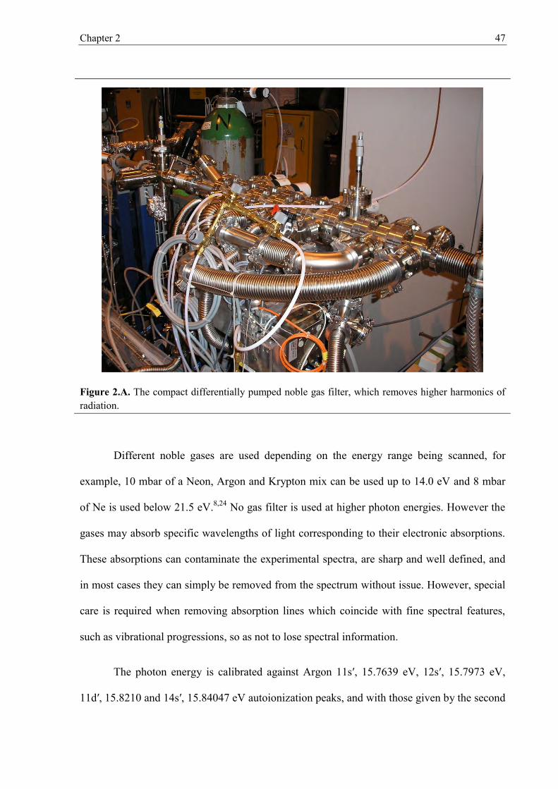
Chapter 2 47

Figure 2.A. The compact differentially pumped noble gas filter, which removes higher harmonics of radiation.

Different noble gases are used depending on the energy range being scanned, for

example, 10 mbar of a Neon, Argon and Krypton mix can be used up to 14.0 eV and 8 mbar

of Ne is used below 21.5 eV.8,24 No gas filter is used at higher photon energies. However the

gases may absorb specific wavelengths of light corresponding to their electronic absorptions.

These absorptions can contaminate the experimental spectra, are sharp and well defined, and

in most cases they can simply be removed from the spectrum without issue. However, special

care is required when removing absorption lines which coincide with fine spectral features,

such as vibrational progressions, so as not to lose spectral information.

The photon energy is calibrated against Argon 11s′, 15.7639 eV, 12s′, 15.7973 eV,

11d′, 15.8210 and 14s′, 15.84047 eV autoionization peaks, and with those given by the second

Chapter 2 48

harmonic at half the energy (see Figure 2.B).25 The photon energy resolution is 3 meV at 10

eV.

Figure 2.B(i). The ion yield of 2P3/2 Ar threshold (first harmonic)

Figure 2.B(ii). The ion yield of 2P3/2 Ar threshold (second harmonic)

Chapter 2 49

2.B. The endstation

The endstation, pictured in Figure 2.C, was constructed by Drs Andras Bodi, Melanie

Johnson, Thomas Gerber, Zsolt Gengeliczki, Bálint Sztáray and Thomas Baer,9 in situ at the

SLS. The pure sample is introduced into the experimental chamber through an effusive source

at room temperature, with typical pressures in the chamber of 2–4·10–6 mbar during

measurement. The background pressure is in the order of 10–7 mbar. Low operating pressures

are necessary because the ions and ejected electrons must be allowed to travel to their

respective detectors unimpeded by background sample gas. The sample is ionized by the

incident monochromatic VUV synchrotron radiation dispersed by a grazing incidence

monochromator.8

Figure 2.C. The iPEPICO experiment. VUV light enters from behind, perpendicular to the electorn/ion flight axis (double headed arrow). The electron signal is recorded with a Roendek DLD40 delay-line-detector, and the ions are recorded using a Jordan C-726 detector.

Chapter 2 50

Following photoionization, the photoelectrons and photoions are accelerated in

opposite directions by a constant extraction field of 20–120 V cm–1. The ejected electrons are

velocity map imaged (VMI) onto the 40×40 mm DLD40 Roentdek position sensitive delay-

line detector, whereby threshold electrons are focused using electrostatic lenses onto a smaller

than 1 mm spot on the centre of with a kinetic energy resolution of 1 meV at threshold. The

mainstay of VMI is that electrons with the same initial velocity (and by consequence, the

same kinetic energy) are focussed onto the same area on the detector regardless of where in

the ionization region they were formed.26 Energetic electrons are detected as rings around the

central threshold electron circle (see Figure 2.D.), where the radii is proportional to their

initial velocity perpendicular to the extraction axis. Using electrostatic plates to focus the

electrons prevents distortion of the image, such as blurring that occurs when imaging using

gridded extraction plates. With grids, image quality is restricted by the size of the ionization

volume.27 With VMI, threshold signal can be obtained from a larger ionization area, without

sacrificing signal quality.26

After acceleration in the 5 cm long 120 V cm–1 primary acceleration region, the ions

undergo a further acceleration to –1800 V, which provides the necessary space focusing

conditions.8 This is achieved using the standard Wiley–McLaren conditions,28 where the

arrival time of the ion is independent of where it was formed in the ionization region. This

means that those ions formed at the top of the ionization region (towards the electron detector)

are born at a more positive potential, ions formed further away, at the bottom of the ionization

region towards the ion detector, at a more negative potential and reach the detector virtually

simultaneously to give the lower and upper TOF distribution limit.15,28 A compromise is

reached between electron energy resolution which decreases with increasing electric field, and

ion mass resolution, which increases with increasing electric field. This is important because

Chapter 2 51

lower electric fields prolong the residence time of the dissociating ion in the acceleration

region, thereby enabling the rate constants to be measured and kinetic shifts to be observed in

instances of slowly (metastable) dissociating ions. This means that where necessary, as in the

in the case of ions formed with large kinetic energy release giving rise to substantially

broadened ion time-of-flight peaks, larger fields can be used to draw out the ions without

sacrificing electron energy resolution. Ions then enter the 55 cm field free drift region and are

finally detected by a Jordan TOF C-726 microchannel plate assembly.8

2.C. Capturing the electron and ion signals

All of the emitted electrons are focussed onto the imaging detector and as previously

described; electrons with low kinetic energy are focussed onto the centre of the detector and

electrons with electronic with significant kinetic energy (hot electrons) are focussed around

this central spot. However some of the hot electrons have a velocity vector that is already

oriented along the flight tube axis and also arrive at the centre of the detector, thereby

contaminating the true threshold signal. As such, there needs to be some discrimination

against hot electrons to yield the true threshold electron signal. One approach is to process the

total signal to yield the threshold signal. Typically, the 3 dimensional expanding Newton

sphere of charged particles is extracted from the 2 dimensional projection (image) as captured

by VMI with techniques such as the onion peeling algorithm,29 inverse Abel transformations8

or pBasex.30 However noise can be generated in the reconstructed image for example, by over

subtracting contributions made by the faster electrons.

Chapter 2 52

Figure 2.D. The electron signal image of 1,1-C2H2F2 at 15.325eV, as captured by the DLD40 position sensitive detector. (a) The image, (b) the circle area where threshold electron signal is located, highlighted blue and (c) the ring area highlighted yellow where the background (hot) electrons are.

Figure 2.E. The threshold electron signal of CH2Cl2

+ as captured by the circle area on the detector plotted with the background (hot) electron contamination as detected by the ring area and the final TPES. The sharp lines at 11.56, 11.76 eV and between 12.5 and 15.5 eV are absorption lines from the gas filter.

In this instance, the hot electron contamination of the threshold signal is accounted for

by a simple subtraction process, as introduced by Sztáray and Baer.31 This method is preferred

over the other techniques because it enables the use of high extraction fields to maximise ion

TOF resolution without sacrificing the quality of the true threshold electron signal.31,32 The

signal, as captured by the delay-line detector, from a small ring around the central spot, is

Chapter 2 53

subtracted from the central threshold signal (see Figure 2.D.). A greater signal to noise ratio,

especially at higher energies where most electrons are very energetic providing an almost

constant background, is produced when the threshold electrons are focused onto the small

circle area, which is typically tenths of a mm in diameter (see Figure 2.E). The true threshold

signal is obtained by subtracting the background hot electron signal (multiplied by a factor

which is the ratio of the two areas) from the threshold central spot signal. In the absence of a

significant rotational envelope in the TPES, this subtraction process yields a true zero energy

electron signal.

Electron hit positions and times, and ion hits, are recorded using a time-to-digital

converter card (HPTDC) operating in a special triggerless mode designed for the experiment.8

This triggerless mode is designed to reduce the number of false coincidences recorded in the

data and to improve the repetition of the experiment, to better correlate with the quasi-

continuous nature of the synchrotron light. In any coincidence experiment, false coincidences

will occur which are caused by the detection of an ion and an electron which were not formed

in the same ionization event. These false coincidences can add considerable noise to the TOF

spectrum reducing its quality.

Count rates supplied by data acquisition methods such as continuous single-

start/single-stop (SS) and single-start/multiple-stop (SM) modes are not suitable for the high

ionization rates produced with synchrotron based experiments. In (SS) data acquisition the

TOF counting stops when the first stop signal is received, making it unsuitable for high

intensity experiments. Start signals are lost while the time-to-amplitude converter (TAC) used

to detect ion hits waits for the stop signal. After this initial stop signal, any additional stops

are lost, so no discrimination between true and false coincidences is made33 and the

background signal drops exponentially from zero time.11,34 In single-start/multiple-stop

Chapter 2 54

(SM)35,36 counting starts after receiving the first start signal and all stops signals are recorded.

Start signals are still lost while the acquisition cycle (using a time-to-digital converter)

completes, and the false coincidence background is no longer constant for high event

frequencies and electron collection efficiencies, and is therefore a limiting factor.

Instead, an alternative scheme is implemented in the iPEPICO apparatus. Time-of-

flight ion distributions are obtained by correlating electrons and ions ‘on the fly’ with a

multistart-multistop (MM) mode of data acquisition, reducing waiting (deadtime). All start

signals are correlated with all stop signals within the relevant time signal, preventing paralysis

of the ion or electron signal,15 to produce a constant background along the TOF spectrum.11

(MM) mode of data acquisition is particularly suited to high intensity synchrotron work, as it

enables data collection with the arbitrarily high ionization rates afforded by the intense

synchrotron light. In pulsed experiments, ions accumulate in the ionization region until they

are pulsed out to the detector which increases the number of false coincidences. Ion signals

originating from false coincidences can be identified by their displacement from the

ionization region and by their increased kinetic energy gained from the extraction pulse, thus

appearing at an earlier TOF. Here, false parent ion coincidences can be distinguished, but it

becomes less clear for false daughter ion signals which are produced with a distribution of

translational energies.37 The pulsed-extraction experimental setup is constrained by the need

to minimize false coincidences whilst maximizing true coincidences, as the expected number

of ionization events needs to be circa one per pulse, which considerably lengthens the data

acquisition time. However, this does not apply with the continuous extraction employed in the

iPEPICO set-up and count rates are limited by the false coincidence background signal.

Chapter 2 55

2.D. The experimental results

The final results derived from the primary experimental data (as given by threshold

electron and ion signals outlined above) are; the threshold ion TOF distributions measured as

a function of photon energy, containing both the fractional ion abundances as well as the rate

information in the form of asymmetric daughter ion peak shapes, and the threshold electron

signal as a function of photon energy. The former can be concisely plotted in the breakdown

diagram, i.e. the fractional ion abundances as a function of the photon energy, which includes

most of the experimental information for fast dissociations. As the relative ratios of the ion

abundances are plotted in the breakdown diagram, the TPEPICO technique is unaffected by

changes in sample pressure, photon flux and varying Franck–Condon factors across photon

energy. Plotting the threshold electron signal yields the threshold photoelectron spectrum

(TPES). All electron counts were normalized to sample pressure (recorded with each point)

and photon flux. The flux delivered to the endstation via the high and low energy diffraction

grating, through the various noble gas filters, was measured by recording the fluorescence

originating from the synchrotron light striking a sodium salicylate coated Pyrex window with

photomultiplier tube.

Chapter 2 56

References

(1) Bodi, A.; Kvaran, Á.; Sztáray, B. J. Phys. Chem. A. 2011, 115, 13443-13451. (2) Borkar, S.; Sztáray, B.; Bodi, A. Phys. Chem. Chem. Phys. 2011, 13, 13009-13020. (3) Bodi, A.; Shuman, N. S.; Baer, T. Phys. Chem. Chem. Phys. 2009, 11, 11013. (4) Hemberger, P.; Noller, B.; Steinbauer, M.; Fischer, I.; Alcaraz, C.; Cunha de Miranda, B.

r. K.; Garcia, G. A.; Soldi-Lose, H. J. Phys. Chem. A. 2010, 114, 11269-11276. (5) Hemberger, P.; Bodi, A.; Schon, C.; Steinbauer, M.; Fischer, K. H.; Kaiserc, C.; Fischerb,

I. Phys. Chem. Chem. Phys. 2012, 14, 11920-11929. (6) ong or . . e e s . asi . odi A. t r ay . l. Organomet. 2012, 31, 3620-

3627. (7) t r ay . l. aer . J. Phys. Chem. A. 2002, 106, 8046-8053. (8) Bodi, A.; Johnson, M.; Gerber, T.; Gengeliczki, Z.; Sztáray, B.; Baer, T. Rev. Sci.

Instrum. 2009, 80, 034101. (9) Johnson, M.; Bodi, A.; Schulz, L.; Gerber, T. Nucl. Instr. and Meth. A. 2009, 610, 597-

603. (10) Sztáray, B.; Bodi, A.; Baer, T. J. Mass. Spectrom. 2010, 45, 1233 - 1245. (11) Bodi, A.; Sztáray, B.; Baer, T.; Gerber, T.; Johnson, M. Rev. Sci. Instrum. 2007, 78,

084102. (12) http://www.psi.ch/sls/about-sls. date accessed 10/03/2012. (13) Hulbert, S. L.; Williams, G. P. Vacuum Ultraviolet Spectroscopy; Academic Press:

London, 2000. (14) Dannacher, J.; Schmelzer, A.; Stadelmann, J.-P.; Vogt, J. Int. J. Mass Spectrom. Ion.

Phys. 1979, 31, 175-186. (15) Eland, J. H. D. Int. J. Mass Spectrom. Ion Proc. 1972, 9, 397-151. (16) Güthe, F.; Locht, R.; Leyh, B.; Baumgärtel, H.; Weitzel, K.-M. J. Phys. Chem. A. 1999,

103, 8404-8412. (17) Locht, R.; Leyh, B.; Dehareng, D.; Hottmann, K.; Baumgärtel, H. J. Phys. B: At. Mol.

Op. Phys. 2010, 43, 015102-015117. (18) Powis, I. Chemical Physics 1983, 74, 421-432. (19) Locht, R.; Dehareng, D.; Leyh, B. J. Phys. B: At. Mol. Op. Phys. 2012, 45, 115101-

115118. (20) Werner, A., S.; Tsai, B. P.; Baer, T. J. Chem. Phys 1974, 60, 3650-3657. (21) Ashfold, M. N. R.; Nahler, N. H.; Orr-Ewing, A. J.; Vieuxmaire, O., P. J. ; Toomes, R.

L.; Kitsopoulos, T. N.; Garcia, I. A.; Chestakov, D. A.; Wuc, S.-M.; Parker, D. H. Phys. Chem. Chem. Phys. 2005, 8, 26-53.

(22) Penfold, T. J.; Spesyvtsev, R.; Kirkby, O. M.; Minns, R. S.; Parker, D. S. N.; Fielding, H. H.; Worth, G. A. J. Chem. Phys 2012, 137, 204310-204322.

(23) Bodi, A.; Hemberger, P.; Gerber, T.; Sztáray, B. Rev. Sci. Instrum. 2012, 83, 083105-083113.

(24) Minnhagen, L.; Palmeri, P.; Biémont, E. NIST Atomic Spectra Database (ver. 5.0). In http://physics.nist.gov/cgi-bin/ASD/energy1.pl; National Institute of Standards and Technology, 2012.

(25) Ralchenku, Y.; Kramida, A. E.; Reader, J.2008 NIST ASD Team, Atomic Spectra Database, NIST, National Institute of Standards and Technology Gaithersburg, MD http://physics.nist.gov/asd3.

(26) Eppink, A. T. J. B.; Parker, D. H. Rev. Sci. Instrum. 1997, 68, 3477-3485. (27) Chandler, D. W.; Houston, P. L. J. Chem. Phys 1987, 87, 1445-1447. (28) Wiley, W. C.; McLaren, I. H. Rev. Sci. Instrum. 1955, 26, 1150-1158. (29) Manzhos, S.; Loock, H.-P. Comp. Phys. Comms. 2003, 154, 76-87. (30) Garcia, G. A.; Nahon, L.; Powis, I. Rev. Sci. Instrum. 2004, 75, 4989-4996. (31) Sztáray, B.; Baer, T. Rev. Sci. Instrum. 2003, 74, 3763-3768. (32) i . t ray . l.; Baer, T. J. Am. Chem. Soc. 2001, 123, 9388-9396.

http://www.psi.ch/sls/about-sls

http://physics.nist.gov/cgi-bin/ASD/energy1.pl;

http://physics.nist.gov/asd3

Chapter 2 57

(33) Baer, T.; Sztáray, B.; Kercher, J. P.; Lago, A. F.; Bodi, A.; Skull, C.; Palathinkal, D. Phys. Chem. Chem. Phys. 2005, 7, 1507-1513.

(34) Baer, T.; Booze, J. A.; Weitzel, K. M. Vacuum Ultraviolet Photoionization and Photodissociation of Molecules and Clusters; World Scientific: Singapore, 1991.

(35) Dutuit, O.; Baer, T.; Metayer, C.; Lemaire, J. Int. J. Mass Spectrom. Ion Proc. 1991, 110, 67-82.

(36) Jarvis, G. K.; Weitzel, K.-M.; Malow, M.; Baer, T.; Song, Y.; Ng, C. Y. Rev. Sci. Instrum. 1999, 70, 3892-3907.

(37) Ng, C. J. Elec. Spec. Rel . Phenom. 2000, 112, 31-46.

Chapter 3 58

Chapter 3:

Theory

Preamble

This chapter is about the computational approaches used in the analysis of the

experimental data. Computational methods have been used within the work presented in this

thesis in combination with the experimental results, to help untangle the dissociation

dynamics, determine thermochemical values and provide a more complete picture of the

potential energy surfaces,

(1) Density functional theory (DFT) methods have been used to calculated molecular

geometries and potential energy paths.

(2) A few selected different composite methods have been used to determine ion

dissociation potentials and thermochemical values.

(3) Using unimolecular rate theory to model the ion breakdown curves produced from

the coincidence experiments to determine 0 K onset energies.

(4) To model the TPES using Franck–Condon factors, and elucidate the geometry of

the cations.

Chapter 3 59

The GAUSSIAN 031 and GAUSSIAN 092 computational suits have been used throughout the

work presented in this thesis. The QChem computational suite3 was used to calculate

ionization levels and excited state potential energy paths shown in Chapter 6 using EOM-IP-

CCSD (equation of motion ionization potential coupled cluster singles and doubles)

methods.4,5

3.A. Computational methods

3.A.1. Calculating molecular geometries and potential energy paths.

Optimized geometries were calculated for the neutral parent molecule, parent

molecular ion, ionic transition states and the ionic and neutral fragments, using density

functional theory (DFT) with the high level of theory and basis set, B3LYP 6-311++G(d,p).

B3LYP6 is the Becke three parameter7 hybrid Lee–Yang–Parr exchange correlation

functional,8 which includes a combination of Hartree–Fock exchange with DFT exchange

correlation. 6-311++G(d,p) is a Pople-type basis set, applicable from hydrogen to krypton,

with each core atomic orbital basis function comprised of six Gaussian primitive functions.

311 corresponds to three contracted basis functions corresponding to each valence atomic

orbital, a triple–ζ basis set. The first one (3) is composed of a linear combination of three

primitive Gaussian functions and the second and third (11) are of a linear combination of

individual primitive Gaussian functions.9 Diffuse functions (++) added to each angular

momentum function of the basis set which describes the sparse distribution of electrons far

from the effects of the nucleus.10 Diffuse s orbital functions are added to hydrogen, and

diffuse s and p orbitals are added to the remaining heavier atoms. The polarization functions

(d,p) have higher angular momentum quantum numbers than the occupied atomic orbitals.

Chapter 3 60

They are used to describe the distortion of the atomic orbitals within a molecule caused by the

interactions with neighbouring atoms, p orbitals are added to the hydrogen, and d orbitals are

added to 2nd row atoms.11

Figure 3.A. Sketch of a 3-dimensional potential energy surface along reaction coordinates q1 and q2.. At both minimums and saddle point (transition state) along coordinate q1, the energy gradients are zero and are termed stationary points.

The optimized geometries were used to supply the various input molecular parameters

required for modelling the breakdown diagrams and TPES. The optimized ion geometries,

which are global minimums or stationary points in the potential energy surface, were used as

the starting points for two types of constrained optimizations to generate reaction paths. The

first is where a bond may be lengthened to between 3 and 5 Å as for dissociation, and the

second where the bond angles can be increased or decreased, as in a rearrangement. The

reaction path scans were used to identify possible sites (energies and geometries) along the

potential energy surface that are transition state regions, in which the true transition state can

be located. Transition states were then accurately located using the TS and Synchronous

Chapter 3 61

Transit-guided Quasi-Newton (STQN) methods; QST2 and QST3 integrated into the

Gaussian computational suite.12,13 The TS method requires an initial guess geometry input for

the transition state, found from the constrained optimization scans. For best results, this

starting geometry should be fairly close to the one that is required. However, QST2 and QST3

do not require such an accurate initial transition state geometry, but simply the start and end

product molecule geometries and in the case of QST3, a less accurate transition state

geometry. Once the optimized geometries of the transitions states were found, composite

calculations were undertaken to accurately determine their thermochemical properties.

3.A.2. Composite methods

Thermochemical values such as bond dissociation energies, enthalpies of formation,

reaction barrier heights and zero-point vibrational energies can be calculated accurately using

a variety of computational methods, all varying in computational cost (time), accuracy and

reliability. The first requirement for such calculations is; all calculations must be performed

using systems whose geometries have been optimized. That is to say, the point on the

potential energy surface at which the first derivative of the energy (the gradient) and hence the

negative of this derivative (the forces) is zero. These points, known as stationary points,

correspond to any minimum (global or local) representing a stable structure, and any saddle

point or transition state (which is a maximum along the reaction coordinate, but a minimum

along all other coordinates) present on the potential energy surface, see Figure 3.A. The most

basic of methods consists of a one-step frequency calculation on an optimized stationary point

where sources of input for determining thermochemical values are the translational,

vibrational, rotational and electronic partition functions. Such input commands typically

Chapter 3 62

comprise of which particular basis set and level of theory one wishes to use, in order to

calculate the vibrational frequencies e.g. a lower level of theory e.g. the wave functional

theory (WFT) Hartree–Fock methods (HF) and basis set such as the minimal STO–3G basis

set (one basis function for each atomic orbital with the sum of 3 Gaussian functions

approximating a Slater type function) or a higher level of theory (e.g. density functional

theory (DFT) with e.g. the B3LYP hybrid functional) and higher basis set with additional

polarization diffuse functions added such as the 6–311+G(d,p) basis set. However, the exact

exchange-correlation functional, i.e. a unique method to accurately calculate enthalpies of

formation or bond dissociation energies using a single determinant alone remains the Holy

Grail in computational chemstry.14 Subsequently modifications have been made, the most

successful of which are in a class of calculations termed composite calculations. Composite

methods consist of combining several steps with varying basis sets and levels of theory in an

attempt to capitalize the effectiveness of a particular basis set but off-set with a lower level of

theory. The aim of such composite methods is to reach a compromise between computational

cost and reliable, highly accurate results to within ~1–10 kJ mol–1. The different types of

density functional theory (DFT) extrapolation based composite methods are the Gn methods;

G2, G3,15 G2B3, G3B3,16 Complete Basis Set (CBS) methods; CBS-QB3, CBS-APNO 17,18,19,

and the hybrid wave function / DFT based Weizmann theory, W120 and W221 . Improvement

to W1 and W2 is given by the wave function based W322 method. Traditional ab initio

quantum chemistry (wave function theory) attempts to improve the reliability and accuracy of

determining the molecular energetics with increasing the accuracy of the wave function, at

considerable computational cost. An overview of the varying accuracy, cost and treatment of

electron correlation across the different methods, from single functional methods like HF and

Chapter 3 63

DFT B3LYP to modern ab initio extrapolation methods such as W1-2.20-22 is shown in Figure

3.B.

The methods used throughout the work presented in this thesis are the composite

method G3B3 and the W1 method. A summary of the main processes involved in each

method are presented below.

The G3B3 composite method is an additive method based on a series of six

calculations performed under one keyword, G3B3 and is a combination of high level theory

and smaller basis sets, with two experimental parameters.15,16

(1) The equilibrium geometry is obtained with density functional theory: B3LYP/6-

31G(d). The equilibrium energies are refined using all electrons for the calculation

of the correlation energies. The geometry is then used as the basis for the

remainder of the calculation. The major difference between the different Gn

methods is highlighted here, the geometry is obtained by HF methods for G3,

whereas DFT is used in G3B3 and G4.

(2) The harmonic frequencies (scaled by a pre-determined factor) are obtained using

the equilibrium geometry, and are used to give the zero point vibrational energy

(ZPE).

(3) A group of single point energies are calculated using the following combination of

second and fourth order Møller–Plesset and quadratic configuration interaction

QCISD(T) levels of theory: MP4(FC)/6-31G(d), MP4(FC)/6-31+G(d),

MP4(FC)/6-31G(2df,p), QCISD(T,FC)/6-31G(d),MP2(FU)/G3large. These

energies are used for a series of four corrections, (a) a correction is applied for

diffuse functions, (b) a correction for higher polarization functions on non-

Chapter 3 64

hydrogen atoms and p-functions on hydrogens, (c) correction for correlation

effects beyond fourth-order perturbation theory and (d) a correction for the effects

of larger basis set and also for non-additivity which is caused by assuming

separate basis set extensions for diffuse functions and higher polarization

functions. Another difference between G3B3 and other Gn theories, is the

combination of what theories are used at this stage; e.g. G3 and G3(MP2) uses

mostly Møller–Plesset perturbation theory, MP2, MP4.

(4) The spin–orbit correction, taken from a combination of experiment and theoretical

calculations where applicable,15 is combined with the above four results from step

(3) for atomic species only.

(5) A ‘higher level correction’ is added which accounts for remaining deficiencies

within the energy calculation utilizing the corrections for paired and unpaired

valence electrons in both atoms and molecules.

(6) Finally, the total energy at 0 K, E0, is derived by summing the ZPE from step 2, to

the result from step 5.

Whilst this method is very accurate for closed shell neutral molecules, it struggles to

accurately calculate thermochemical values for molecules containing heavy atoms and open

shell species such as cations.

Chapter 3 65

Figure 3.B. Diagram showing the increasing accuracy across the range of avaliable ab initio methods to accurately calculate thermodynamic properties, towards the exact value.

The experimentally derived components of the Gn methods can carry in themselves

large uncertainties that are too large to be acceptable for a highly accurate system. Weizmann

theory, W1 is based on extrapolation to the complete basis set limit, with separate

extrapolations of SCF (self-consistent field, HF), CCSD (coupled cluster with all connected

singles and doubles)23 and (T) (perturbative triple excitation effects)24 components was

developed. W1 has no empirical parameters, empirical additivity corrections and other

corrections which are derived, often achieving an accuracy of less than 0.3 kcal mol–1 or ca. 1

kJ mol–1. The W1 protocol is outlined as follows;

(1) The geometry is optimized at the B3LYP/VTZ+1 level

(2) Harmonic frequencies are obtained from the geometry optimization, the ZPE

calculated and scaled by a factor

(3) Single point calculations using coupled cluster methods; CCSD(T)/AVDZ+2d and

CCSD(T)/AVDZ+2d1f

Chapter 3 66

(4) Another single point calculation using CCSD(T)/AVQZ+2d1f is made

(5) The SCF component of total electronic energies is extrapolated

(6) The CCSD valence correlation component is derived

(7) The (T) valence correlation component is derived

(8) The contributions to core correlation are obtained at the CCSD(T) level with the

smallest Martin–Taylor basis set (MTvtz, denoted simply as MT).

(9) Finally, scalar relativistic and spin–orbit coupling effects are treated at the

ACPF/MT (averaged coupled pair functional) small level.25 This basis set is the

best compromise between quality and computational expense, which is mostly

consumed by the core correlation calculations.20,21

However, the W1 method is optimized for row 1 and 2 elements and heavier atoms are

excluded.26

Other advancements include the formulation of the high accuracy extrapolated ab

initio thermochemistry, HEAT,27 protocol based on the Weizmann theories and large basis

sets which is a wave function method devoid of all empirical scaling factors and

adjustments.28 The next step in development is the method as used by Csontos et al.,29 which

is based upon a combination of W3 and HEAT. However, these advancements delivering

thermochemical accuracies of less than 1 kJ mol–1 come at considerable computational cost.

Chapter 3 67

3.B. Modelling

3.B.1. Modelling the breakdown curves

The experimental breakdown curves were modelled using the program developed by

Sztáray et al.30 The program was used to model both slow and fast dissociations. Both the ion

time-of-flight distributions and the breakdown curves are modelled using the following fixed

parameters; the thermal energy distribution, ionization energy, the parameters which affect the

ion TOF i.e. ion acceleration fields and the acceleration and drift distances, and ion

vibrational frequencies to determine the density of states of the dissociating ion. The

vibrational frequencies of the transition state determine the entropy of activation. Within the

Rigid Activated Complex (RAC-)-RRKM framework used throughout this work, selected

vibrational modes (the transitional modes) which turn into overall rotational modes of the

product ion are scaled by a constant; five frequencies are scaled for the loss of a neutral with

3-D rotations, four for the loss of a linear fragment and two for atom loss.30 As the low

transitional frequencies are scaled, determining their precise values with ab initio calculations

is not necessary.

By altering the barrier height and scaling the transition state frequencies, the number

and density of states available to the reaction are changed. Altering the temperature changes

the width of the ion internal energy and the width of the crossover section of the breakdown

curves (where 50% of parent ions dissociate into fragment daughter ions, starting at the

energy range where the parent ion signal initially decreases to where it disappears, the E0 of a

fast reaction), in other words, the slope of the approach to E0. A higher temperature will

broaden the crossover region. A lower temperature will narrow the region, producing a

sharper approach to E0. The actual value of E0 itself is independent of the temperature.31,32

Chapter 3 68

The temperature dependence of the breakdown curves means they are effectively a molecular

thermometer, measuring the temperature of the neutral molecule.33 Altering the transition

state frequencies effects the density of states; lowering the transition state frequencies

increases the reaction rates and increasing them decreases reaction rates.

In some instances the IE may also be varied to reproduce the breakdown diagram, as is

the case for the fast dissociation of CFBr3+.34 In these instances the ionization potential value

supplied from the literature may not be suitable and could have been inaccurately determined

from fairly ambiguous photoelectron spectra. As such the IE may also be fitted, providing a

better fit to the experimental data around the onset energy as well as an improved value for

the IE.34 The general process for modelling the breakdown diagram and ion TOF distributions

is given in Figure 3.C.

3.B.1.1. Fast dissociations

The E0 for a fast dissociation into the first daughter ion (lowest dissociation channel)

is found where the parent ion signal reaches zero. It is assumed that the neutral thermal

distribution is faithfully transposed onto the ion manifold, i.e. every parent ion with more

internal energy than the dissociation threshold results in a fragment ion. The fractional

abundance of the parent ion plotted as a function of photon energy (the breakdown curve)

corresponds to the cumulative distribution function (CDF) of the ion internal energy with the

dissociation energy as the integration limit, and by inference the CDF of the neutral internal

energy at the experimental temperature. The ratio of the parent ion signal is given by;

Chapter 3 69

( ) ∫ ( )

∫ ( )

(3.1)

where Pi is the normalized internal energy distribution of the parent ion as a function of the

internal and photon energies. Pn is the internal energy of the neutral molecule which can be

calculated using the Boltzmann formula; Pn (E) = ρn(E)•e–E/kT where ρn is the density of states

of the neutral molecule, calculated using the molecules vibrational frequencies and rotational

constants determined with ab initio calculations. At hv = E0 – IE the above integral becomes

zero and the disappearance of the parent ion signal gives the 0 K dissociation onset energy. In

other words, E0 is reached when no part of the thermal distribution is contained within the

bound part of the ion potential energy curve any more, but has progressed above the

dissociation limit.

The breakdown diagram of a fast dissociation at 0 K should be a step function, where

the parent ion signal drops instantly from 100% to 0% and the daughter ion signal increases

from 0% to 100% at the dissociation limit. In practice, the finite resolution of both the

electron and photon spectrometers, together with the molecules thermal distribution of

internal energies, means the ion yield curves deviate from the step-function ideal. Instead, the

cross-over region can be as large as several hundred meV. However, modelling this

breakdown diagram is necessary when the disappearance of the parent ion is poorly defined.

Furthermore, modelling the breakdown diagram can supply information about the shape of the

potential energy surface by telling us if the neutral thermal distribution is fully accommodated

onto the bound part of the ion manifold i.e. into the deep well, before dissociation occurs, or

not. If the width of the thermal energy distribution is greater than the depth of the well, then

low energy neutrals do not produce ions, and the well is deemed shallow. This is expanded

upon in Chapter 4.

Chapter 3 70

Figure 3.C. Schematic of the breakdown diagram modelling process. Ab initio calculations provide the input, fast dissociations only require the room temperature ion internal energy distribution whereas slow dissociations also require the ion density of states and the number of states supplied by the transitions state geometry. Ion time-of-flight (TOF) distributions must be fitted to obtain accurate reaction rates and reproduce the breakdown curves. Experimental parameters include the temperature and the dimensions of the experiment.

Chapter 3 71

The breakdown diagram can be modelled by considering the thermal energy

distribution of the neutral molecule, which yields the energy distribution of the ion as a

function of photon energy. Frequencies for the ion and neutral were taken from calculations,

as outlined in section 3.A.1. The only parameters which can be altered to accurately determine

E0 is the barrier height, the temperature and in a small handful of cases the IE value.

3.B.1.2. Slow dissociations

The window of dissociation rates of iPEPICO, in which the absolute rate constants are

measurable, is 103 s–1 < k < 107 s–1. Above 107 s–1, the dissociation occurs too swiftly to

measure the rate, and below 103 s–1 the dissociation is not accommodated within the time

frame of the iPEPICO experiment. As a result of this physical constraint, the slowly

dissociating ions do not have enough time to fragment before reaching the detector.

Consequently, the ion TOF distribution is not a single narrow Gaussian-type peak, but one

that has a diminishing quasi-exponential tail, towards longer TOF times. The whole signal of

this metastable ion is attributed to dissociations occurring during the course of acceleration.

The signal from metastable daughter ions born in the remainder of the flight tube is so

smeared out up to the parent ion TOF limit and is barely perceptible, see Figure 3.D.

For slow dissociations, the true 0 K onset is not found by inspection of the breakdown

diagram where the parent ion signal disappears, but is somewhat lower in energy. A second

integral, the ion energy distribution function multiplied by the analytical solution to the

differential equation of the unimolecular kinetics, needs to be included giving the equation

below,30

Chapter 3 72

( ) ∫ ( )

∫ ( ) ( ( ) )

(3.2)

here k(E) is the internal energy-dependant rate constant and τmax is the maximum flight time

within which the parent ion has to dissociate into the fragment ion in order to be detected as

fragment ion.30 The fragment ion fractional abundance is then given by 1 minus the

abundance of the parent ion;

( ) ∫ ( ) ( ( ( ) ))

(3.3)

Modelling the breakdown diagram requires the dissociation rate constants to be taken

into account; these can be extracted from the ion TOF distributions. The fragment ion peak

shape is given as,

( ) ∫ ( ) ( ( ( ) ( )) ( ( ) ( )))

(3.4)

The normalized height of the ion peak channel is given by Fri(hv), P(E,hv) is the internal

energy distribution of the parent ion, τ is the dissociation time, and τ(TOF) is the time

corresponding to the time of flight channel, i. The sharp TOF spectrum is convoluted with a

Gaussian distribution to account for thermal broadening or kinetic energy release, to give the

final TOF spectrum.30

Chapter 3 73

Figure 3.D. Schematic of the coincidence setup. The metastable daughter D+1 is formed very slowly

throughout the acceleration region in a quasi-exponential fashion. Any ions including the parent ions, P+ that are formed at the ionization region produce a symmetrical TOF distribution.

The modelled breakdown curves are determined by using the thermal energy

distribution of the molecule and an assumed dissociation rate function, k(E) obtained using

statistical RAC-RRKM theory. The adjustable parameters become the barrier height (giving

the 0 K onset), the transition state vibrational frequencies and the temperature. A unique k(E)

function is obtained from fitting the experimental TOF distributions which is used in

conjunction with fitting the other parameters to obtain E0.30 The metastable ion TOF peak

distribution depends on the absolute dissociation rate, but the breakdown diagram depends on

the ratio of rate constants for parallel dissociations. Therefore it is the fitting of the TOF

distributions which is most affected by changing the transition state frequencies, and the

shape of the breakdown diagram is less affected.

Chapter 3 74

3.B.1.3. Parallel and consecutive reactions

Parallel reactions are those dissociation reactions giving more than one set of product

fragments, which are derived from the same parent ion molecule and occurring

simultaneously;

ABC + hv – e– → ABC+ → AB+ + C Primary dissociation channel (1) (3a)

ABC + hv – e– → ABC+ → A + BC+ Parallel dissociation channel (2) (3b)

The experimental data supplies the relative rates of dissociation which have to be modelled in

order to derive the E0 of the latter parallel reactions (3b). As the photon energy approaches E0

from above, the rate constant decreases to the limit dictated by the density of states of the ion

at the E0 internal energy. The appearance energy is then given by extrapolation. It is necessary

to model the primary dissociation of the parent ion and the resulting breakdown diagram gives

the ratio of the dissociation rates in the energy region in which the two processes (the primary

and parallel reaction) compete, equation (3.5). The relative rates are therefore a function of

the number of states of the two transition states;

( )

( ) ( )

( )

(3.5)

N1‡ (E – E1) is the sum of the internal energy states in transition state for the reaction 1 from 0

to E – E1. N2‡ (E – E2) is the corresponding quantity for the parallel reaction. This gives the

derived model rate curve for the parallel onset from which the rate is found. As for the

primary dissociation, extrapolation to where the rate curve vanishes gives E0, which is often

Chapter 3 75

below the energy at which the increasing signal in the breakdown diagram is observed. Within

the rigid-activated-complex (RAC) RRKM framework used to model the parallel onsets in

Chapter 5 two parameters are required, (1) the difference of the two E0 values, and (2) the

activation entropy difference (derived from the low vibrational modes of the transition state)

to determine the shape, or more specifically the slope of the breakdown curves. If the

transition state is loose then the slope has a steeper gradient, conversely if the transition state

is tight then the slope is shallower. Overall, because the shape of the breakdown curve for the

parallel reaction is determined by these two parameters, the slope of the onset for the second

reaction channel is gentler than the sharper onsets for the primary dissociation reactions. If the

reaction is fast, then no experimental information about the absolute rates is supplied. In this

instance the vibrational frequencies of one of the transition states is fixed, and the other is

varied to fit the relative rates.35 It must be remembered that as the onset is more gentle, the

precision by which the E0 is determined is reduced, and a greater error must be assigned to it.

Subsequent dissociations of primary daughter ions into further smaller mass ions are

termed sequential reactions.

ABC + hv → ABC+ + e– Ionization (3c)

ABC+ → AB+ + C Primary dissociation channel (3d)

AB+ → A+ + B Sequential channel (3e)

The treatment of such reactions is different from the above parallel reactions. If the sequential

reaction is fast, the yield of the tertiary ion depends upon the energy partitioning in the

products of the primary dissociation channel. Similarly, this too can be modelled with

statistical theory by assuming that excess energy after dissociation is statistically partitioned

amongst the vibrational, rotational and translational degrees of freedom of the primary

products AB+ and C.36 This means that the breakdown curve of A+ can be modelled using

Chapter 3 76

only the rotational degrees of freedom and vibrational frequencies of the AB+ and C products,

which can be calculated using ab initio methods. The properties of the transition state are

ignored.35 The product ion distribution of A+ for reaction (3e) formation of A+ + B + C, has a

broader internal energy distribution because excess energy is partitioned into both AB+ and C

fragments (reaction 3d).37 This manifests itself in the breakdown diagram as a broad and

gently curving onset. If the reaction is slow, then fitting both the breakdown diagram and the

asymmetric ion TOF distributions of A+ limits the acceptable range of E0, meaning it can be

determined with a greater precision than the fast parallel dissociations mentioned above.35

3.B.2. Modelling the TPES

Modelling the TPES using Franck–Condon factors (FCF), the square of the overlap

integrals of the ion and neutral wavefunctions, provides the link between ground electronic

states of the neutral molecule and its cation. By fitting the TPES, the transition probabilities

for ionization into each possible final vibrational state of the ground electronic ion state can

be obtained. Noting how the FCFs change with varying cation geometry to provide the best fit

to the TPES, can provide us with the best geometry for the cation.

Calculating the FCFs requires the geometries of both the neutral and ion molecules.

Highly accurate density functional theory (DFT, B3LYP/6–311++G(d,p)) calculations were

performed using the GAUSSIAN 03 suite of programs to obtain the geometry and vibrational

frequencies of the ground state neutral, as well as that of the ground state cation. The program

‘FCfit v2.8.8’ was used to simulate and fit the TPES.38 A schematic of the modelling

procedure is given in Figure 3.E. The program computes the FC integrals of multidimensional

harmonic oscillators based on the recursion formula of Doktorov, Malkin and Man’ko.39,40

Chapter 3 77

Figure 3.E. Schematic of the process of modelling the TPES. Ab initio calculations and the experimental data provide the input. Outputs are the convoluted stick spectrum and subsequent new ion geometry.

The normal coordinates of the ground neutral and ground ion electronic state are

related by the linear orthogonal transformation given by Duschinsky, where the normal

coordinate of the neutral is given by the normal coordinate of the ion multiplied by the

rotation matrix which turns the coordinate system of one state into another, plus the

displacement vector.41

Chapter 3 78

In the first stage, the program FCfit v2.8.8 reads the vibrational coordinates from the

optimized geometries for the neutral and cation molecules, together with the ab initio force

constant matrices, to calculate a stick spectrum of the possible vibrational progressions based

on the normal modes of vibration. Cursory intensities are based upon the initial input neutral

and cation geometries, with a vibrational temperature of 0 K. This stick spectrum is used to

help assign the peaks in the TPES, as all transitions with non-zero FC intensity are

simultaneously given irrespective of their magnitude. As only relative energies of the

transitions are determined, the stick spectrum can be aligned to the experimental TPES by the

addition of the adiabatic ionization energy. In the second stage, the relative intensities of the

vibrational peaks in the major progression (up to a maximum of 10 quanta) are fitted to the

experimental intensities by fine tuning the cation geometry; followed by subsequent fitting of

the intensities of the weaker progressions. It is accepted generally that ab initio methods are

much more robust, accurately describing the potential energy surface for closed shell neutral,

than for open shell species. As such, it is the cation geometries which are optimized and the

neutral geometry remains unaltered. Finally, the stick spectrum is convoluted with a Gaussian

function to simulate the rotational envelope and experimental resolution generating a

comparable spectrum to the experimental spectrum. Peaks arising from vibronic coupling

(Herzberg – Teller)42 can be accommodated because the geometries of the ion state are not

fixed and are allowed to change. However, as the program uses the properties of harmonic

oscillator eigenfunctions, the effects of anharmonicity on the vibrational spacing are not

included. Though the program ‘FCfit v2.8.8’ is to some degree a black box program, some

diligence is required to ensure that the correct optimized geometry inputs for both neutral and

ion are supplied. The FCF calculation is sensitive to the methods used to calculate the

optimized geometries of the neutral and ion states; as such the same method needs to be used

Chapter 3 79

for both calculations. In the event of an unexpected geometry change upon ionization, the

result can be tested by supplying various optimized cation geometries, and only altering the

intensities of the vibrational progressions which do and do not affect the fit. Despite the

success of fitting the ground electronic states, fitting the TPES of excited states is more

difficult as the geometry of the excited state cation may greatly differ from the neutral

geometry. In addition to the difference in geometries, other processes, such as vibronic

coupling may be at play, complicating the spectrum.

Chapter 3 80

References

(1) Frisch, M. J.; Trucks, G. W.; Schlegel, H. B.; Scuseria, G. E.; Rob, M. A.; Cheeseman, J. R.; Montgomery Jr., J. A.; Vreven, T.; Kudin, K. N.; Burant, J. C.; Millam, J. M.; Iyengar, S. S.; Tomasi, J.; Barone, V.; Mennucci, B.; Cossi, M.; Scalmani, G.; Rega, N.; Petersson, G. A.; Nakatsuji, H.; Hada, M.; Ehara, M.; Toyota, K.; Fukuda, R.; Hasegawa, J.; Ishida, M.; Nakajima, T.; Honda, Y.; Kitao, O.; Nakai, H.; Klene, M.; Li, X.; Knox, J. E.; Hratchian, H. P.; Cross, J. B.; Bakken, V.; Adamo, C.; Jaramillo, J.; Gomperts, R.; Stratmann, R. E.; Yazyev, O.; Austin, A. J.; Cammi, R.; Pomelli, C.; Ochterski, J. W.; Ayala, P. Y.; Morokuma, K.; Voth, G. A.; Salvador, P.; Dannenberg, J. J.; Zakrzewski, V. G.; Dapprich, S.; Daniels, A. D.; Strain, M. C.; Farkas, O.; Malick, D. K.; Rabuck, A. D.; Raghavachari, K. J.; Foresman, J. B.; Ortiz, J. V.; Cui, Q.; Baboul, A. G.; Clifford, S.; Cioslowski, J.; Stefanov, B. B.; Liu, G.; Liashenko, A.; Piskorz, P.; Komaromi, I.; Martin, R. L.; Fox, D. J.; Keith, T.; Al-Laham, M. A.; Peng, C. Y.; Nanayakkara, A.; Challacombe, M.; Gill, P. M. W.; Johnson, B.; Chen, W.; Wong, M. W.; Gonzalez, C.; Pople, J. A. Gaussian, Inc., Wallingford, CT, 2003.

(2) Frisch, M. J.; Trucks, G. W.; Schlegel, H. B.; Scuseria, G. E.; Robb, M. A.; Cheeseman, J. R.; Scalmani, G.; Barone, V.; Mennucci, B.; Petersson, G. A.; Nakatsuji, H.; Caricato, M.; Li, X.; Hratchian, H. P.; Izmaylov, A. F.; Bloino, J.; Zheng, G.; Sonnenberg, J. L.; Hada, M.; Ehara, M.; Toyota, K.; Fukuda, R.; Hasegawa, J.; Ishida, M.; Nakajima, T.; Honda, Y.; Kitao, O.; Nakai, H.; Vreven, T.; Montgomery, J., J. A. ; Peralta, J. E.; Ogliaro, F.; Bearpark, M.; Heyd, J. J.; Brothers, E.; Kudin, K. N.; Staroverov, V. N.; Kobayashi, R.; Normand, J.; Raghavachari, K. J.; Rendell, A.; Burant, J. C.; Iyengar, S. S.; Tomasi, J.; Cossi, M.; Rega, N.; Millam, N. J.; Klene, M.; Knox, J. E.; Cross, J. B.; Bakken, V.; Adamo, C.; Jaramillo, J.; Gomperts, R.; Stratmann, R. E.; Yazyev, O.; Austin, A. J.; Cammi, R.; Pomelli, C.; Ochterski, J. W.; Martin, R. L.; Morokuma, K.; Zakrzewski, V. G.; Voth, G. A.; Salvador, P.; Dannenberg, J. J.; Dapprich, S.; Daniels, A. D.; Farkas, Ö.; Foresman, J. B.; Ortiz, J. V.; Cioslowski, J.; Fox, D. J. Gaussian 09, Revision A.1 2009.

(3) Shao, Y.; Molnar, L. F.; Jung, Y.; Kussmann, J.; Ochsenfeld, C.; Brown, S. T.; Gilbert, A. T. B.; Slipchenko, L. V.; Levchenko, S. V.; O’Neill, D. P.; Jr, R. A. D.; Lochan, R. C.; Wang, T.; Beran, G. J. O.; Besley, N. A.; Herbert, J. M.; Lin, C. Y.; Voorhis, T. V.; Chien, S. H.; Sodt, A.; Steele, R. P.; Rassolov, V. A.; Maslen, P. E.; Korambath, P. P.; Adamson, R. D.; Austin, B.; Baker, J.; Byrd, E. F. C.; Dachsel, H.; Doerksen, R. J.; Dreuw, A.; Dunietz, B. D.; Dutoi, A. D.; Furlani, T. R.; Gwaltney, S. R.; Heyden, A.; Hirata, S.; Hsu, C.-P.; Kedziora, G.; Khalliulin, R. Z.; Klunzinger, P.; Lee, A. M.; Lee, M. S.; Liang, W.; Lotan, I.; Nair, N.; Peters, B.; Proynov, E. I.; Pieniazek, P. A.; Rhee, Y. M.; Ritchie, J.; Rosta, E.; Sherrill, C. D.; Simmonett, A. C.; Subotnik, J. E.; III, H. L. W.; Zhang, W.; Bell, A. T.; Chakraborty, A. K.; Chipman, D. M.; Keil, F. J.; Warshel, A.; Hehre, W. J.; III, H. F. S.; Kong, J.; Krylov, A. I.; Gill, P. M. W.; Head-Gordon, M. Phys. Chem. Chem. Phys. 2006, 8, 3172-3191.

(4) Kállay, M.; Gauss, J. J. Chem. Phys 2004, 121, 9257. (5) Landau, A.; Khistyaev, K.; Dolgikh, S.; Krylov, A. I. J. Chem. Phys 2010, 132, 014109-

001422. (6) Stephens, P. J.; Devlin, F. J.; Chabalowski, C. F.; Frisch, M. J. J. Phys. Chem. 1994, 98,

11623-11627. (7) Becke, A. D. J. Chem. Phys 1993, 98, 5648-5652. (8) Lee, C.; Yang, W.; Parr, R. G. Phys. Rev. B. 1988, 37, 758-789. (9) McLean , A. D.; Chandler, G. S. J. Chem. Phys 1980, 72, 5639-5649. (10) Clark, T.; Chandrasekhar, J.; Spitznagel, G. W.; Schleyer, P. v. R. J. Comp. Chem. 1983,

4, 294-301. (11) Frisch, M. J.; Pople, J. A.; Binkley, J. S. J. Chem. Phys 1984, 80, 3265-3270. (12) Peng, C.; Schlegel, H. B. Israeli J. of Chem. 1993, 33, 449-454.

Chapter 3 81

(13) Peng, C.; Ayala, P. Y.; Schlegel, H. B.; Frisch, M. J. J. Comp. Chem. 1995, 17, 49-56. (14) Lazarou, Y. G.; Prosmitis, A. V.; Papadimitriou, V. C.; Papagiannakopoulos, P. J. Phys.

Chem. A. 2001, 105, 6729-6742. (15) Curtiss, L. A.; Raghavachari, K.; Redfern, P. C.; Rassolov, V.; Pople, J. A. J. Chem. Phys

1998, 109, 7764-7776. (16) Baboul, A. G.; Curtiss, L. A.; Redfern, P. C.; Raghavachari, K. J. J. Chem. Phys 1999,

110, 7650-7657. (17) Montgomery Jr, J. A.; Ochterski, J. W.; Petersson, G. A. J. Chem. Phys 1994, 101, 5900-

5910. (18) Ochterski, J. W.; Petersson, G. A.; Montgomery Jr, J. A. J. Chem. Phys 1996, 104, 2598-

2620. (19) Montgomery Jr, J. A.; Frisch, M. J.; Ochterski, J. W.; Petersson, G. A. J. Chem. Phys

1999, 110, 2822-2828. (20) Martin, J. M. L.; de Oliveira, G. J. Chem. Phys 1999, 111, 1843-1856. (21) Parthiban, S.; Martin, J. M. L. J. Chem. Phys 2001, 114, 6014-6029. (22) Boese, A. D.; Oren, M.; Atasoylu, O.; Martin, J. M. L.; Kállay, M.; Gauss, J. J. Chem.

Phys 2004, 120, 4129-4142. (23) Purvis, G. D.; Bartlett, R. J. J. Chem. Phys 1982, 76, 1910-1919. (24) Raghavachari, K.; Trucks, G. W.; Pople, J. A.; Head-Gordon, M. Chem. Phys. Letts.

1989, 157, 479-483. (25) Gdanitz, R. J.; Ahlrichs, R. Chem. Phys. Letts. 1988, 143, 413-420. (26) Karton, A.; Martin, J. M. L. J. Chem. Phys 2012, 136, 124114-124126. (27) Harding, M. E.; Vázquez, J.; Ruscic, B.; Wilson, A. K.; Gauss, J.; Stanton, J. F. J. Chem.

Phys 2008, 128, 114111-114126. (28) Tajti, A.; Szalay, P. G.; Császár, A. G.; Kállay, M.; Gauss, J.; Valeev, E. F.; Flowers, B.

A.; Vázquez, J.; Stanton, J. F. J. Chem. Phys 2004, 121, 11599-11613. (29) Csontos, J.; Rolik, Z.; Das, S.; Kállay, M. J. Phys. Chem. A. 2010, 114, 13093-13103. (30) Sztáray, B.; Bodi, A.; Baer, T. J. Mass. Spectrom. 2010, 45, 1233 - 1245. (31) Borkar, S.; Sztáray, B. J. Phys. Chem. A. 2010, 114, 6117. (32) Kercher, J. P.; Stevens, W.; Gengeliczki, Z.; Baer, T. Int. J. Mass Spectrom. 2007, 267

159-166. (33) Baer, T.; Booze, J. A.; Weitzel, K. M. Vacuum Ultraviolet Photoionization and

Photodissociation of Molecules and Clusters; World Scientific: Singapore, 1991. (34) Bodi, A.; Kvaran, Á.; Sztáray, B. J. Phys. Chem. A. 2011, 115, 13443-13451. (35) Baer, T.; Sztáray, B.; Kercher, J. P.; Lago, A. F.; Bodi, A.; Skull, C.; Palathinkal, D.

Phys. Chem. Chem. Phys. 2005, 7, 1507-1513. (36) Baer, T.; Hase, W. L. Unimolecular Reaction Dynamics: Theory and Experiments;

Oxford University Press Inc.: New York, 1996. (37) S t r ay, B. l.; Baer, T. J. Phys. Chem. A. 2002, 106, 8046-8053. (38) Spangenberg, D.; Imhof, P.; Kleinermanns, K. Phys. Chem. Chem. Phys. 2003, 5, 2505–

2514. (39) Doktorov, E. V.; Malkin, I. A.; Man’ko, V. I. J. Mol. Spec. 1975, 56, 1-20. (40) Doktorov, E. V.; Malkin, I. A.; Man’ko, V. I. J. Mol. Spec. 1977, 64, 302-326. (41) Duschinsky, F. Acta Physicochimica U.R.S.S. 1937, 7, 551-556. (42) Herzberg, G.; Teller, E. Z. Phys. Chem. B. 1933, 21, 410.

Chapter 4 82

Chapter 4:

Fast dissociations of halogenated methanes: a

thermochemical network.

Preamble

The work presented in this chapter has been published as a journal article entitled ‘A

Halomethane Thermochemical Network from iPEPICO Experiments and Quantum Chemical

Calculations’ in 2012 by J. Harvey, R. P. Tuckett and A. Bodi, in the Journal of Physical

Chemistry A, volume 116, issue 39, pages 9696-9705. The majority of the data collection and

analysis was performed by the author, however, the assistance lent by Ms Nicola Rogers, Drs

Mathew Simpson Andras Bodi, Melanie Johnson and Professor Richard Tuckett during

beamtime with the collection of the data is gratefully acknowledged. The modelling program

was developed by B. Sztáray, A. Bodi and T. Baer.1 The threshold photoelectron spectra can

be found in Appendix III.

4.A. Introduction

This chapter focuses on the study of fast dissociations of halogenated methanes using

threshold photoion photoelectron coincidence techniques. It will be demonstrated how the

Chapter 4 83

primary piece of information yielded from such experiments, the 0 K onset energy E0 for the

production of the first photodissociation daughter ion, can be used to construct a network

comprised of enthalpies of formation of neutral and ion species from which more updated and

new thermochemical values can be derived.

Eleven enthalpies of formation are updated, including that for CBrClF2. Importantly,

enthalpies of formation reported in the literature for several neutral and ion species which

were derived using purely computational methods are also confirmed.

Calculations were performed using the GAUSSIAN 09 computational suit.2 Rate

constants calculated with Rice–Ramsperger–Kassel–Marcus (RRKM) theory at arbitrarily

chosen transition state geometries along the dissociation coordinate show that the

dissociations were confirmed to be fast (rates in excess of 107 s–1). Fast dissociative

photoionization processes in threshold PEPICO experiments are modelled simply by taking

into consideration the thermal energy distribution of the neutral molecule, which yields the

energy distribution of the ion as a function of photon energy.1

G3B33 and W14 composite methods (see Chapter 3) were used to determine the

neutral and ion energetics, which were utilised along with previously reported energies5 in the

construction of the thermochemical network shown in section 3.B.4. The experimental onset

energies in the thermochemical network provide rigid links between the neutral and the ion

enthalpies of formation. In the shallow well instances, the initial abundance of the first

daughter ion is non-zero. Even in such cases, the fit was required to reproduce the

disappearance energy range of the parent signal, thus giving the E0 value. The photon energy,

at which the deep well approximation fails, then yields the adiabatic IE.

Chapter 4 84

Quantum chemical calculations on small molecules can yield thermochemical values

with a few kJ mol–1 uncertainties or better, often outperforming experimental results.5-9

Recent threshold photoelectron photoion coincidence (TPEPICO) experiments, in which both

the photon and the photoelectron energies are known to within 1–2 meV (0.1–0.2 kJ mol–1),

1,10-12 are capable of measuring dissociative photoionization onset energies in small to medium

sized molecules with such levels of accuracy. To reiterate, in the absence of an overall reverse

barrier, the onset energies, E0, correspond to the reaction energy at 0 K, and yield the

enthalpies of formation for the parent ion, daughter ion or neutral fragment if two out of the

three are known;

[ ] [ ] [ ] (4.1)

Recent advances in ab initio methods can be rigorously tested and confirmed by

results derived from experiment. The two approaches are, thus, complementary and can be

applied simultaneously to provide sturdier results. For example, experiment can be used to

confirm the highly accurate enthalpies of formation derived by Csontos et al.,5 for a

comprehensive range of neutral halogenated methanes, which were inspired by the W3 and

HEAT protocols.13,14

In threshold photoelectron photoion coincidence, unimolecular dissociation reactions

of internal energy selected parent ions are studied as a function of photon energy, yielding

daughter ion appearance energies.15 Ions are mass analysed in delayed coincidence with

threshold electrons, and the breakdown diagram is generated by plotting the fractional

abundance of parent and fragment ions as a function of hν. For a fast dissociation, every

parent ion with more internal energy than the dissociation threshold results in a fragment ion,

and the breakdown curve of the parent ion corresponds to the cumulative distribution function

(CDF) of the ion internal energy to the dissociation energy. In the first approximation, it

Chapter 4 85

follows that the breakdown curve corresponds to the CDF of the internal energy of the neutral

at the experimental temperature:

( ) ∫ ( ) ∫ ( )

(4.2)

where Pi is the normalised internal energy distribution of the parent ion as a function of the

internal and photon energies. Pn is the internal energy distribution of the neutral molecule,

calculated using the Boltzmann formula Pn(E) = ρn(E) · e–E/kT, where ρn(E) is the density of

states of the neutral.

The above integral vanishes at hν = E0. Consequently, the 0 K appearance energy, E0,

is given by the disappearance energy of the parent ion in small molecules, and modelling the

breakdown diagram only requires the internal energy distribution of the neutral precursor.1

Two assumptions are made when modelling the breakdown curve. First, the neutral internal

energy distribution is transposed directly onto the ion manifold; in other words the threshold

ionization cross sections for the sequence transitions are constant over the thermal energy

range, and there is a uniform probability of threshold ionization across the neutral molecule’s

energy distribution.1,12,16 The Franck–Condon factors for sequence transitions in small

molecules at room temperature are dominated by rotational contributions and this assumption

will hold true as long as the geometries of the neutral and parent ion are sufficiently similar.

However, it is important to note that no assumption is made about the Franck–Condon factors

for threshold ionization as a function of photon energy. Second, the second integral in Eq.

(4.2) assumes that zero internal energy neutrals always contribute to the parent ion signal.

This is only valid if the ground state potential well is deep enough to accommodate the

transposition of the entire thermal energy distribution of the neutral onto the ion manifold in

the photon energy range of the breakdown diagram, which will be termed the ‘deep well

Chapter 4 86

assumption’ (Figure 4.A). However, if the width of the thermal energy distribution is larger

than the depth of the potential energy well, the low energy neutrals do not contribute to the

ion signal. Now, the ‘deep well assumption’ is no longer valid and what we term a ‘shallow

well reality’ prevails. In such cases, the parent signal is always less than 100%, and there is

significant daughter ion signal, even at the ionization limit. This effect had been observed

previously,17 and was first discussed in the TPEPICO study of CFBr3 and CBr4.11

Figure 4.A. Schematic showing the deep well and the shallow well scenarios. As the photon energy (hν) is scanned, the parent ion (AB+) fractional abundance corresponds to the normalized parent ion internal energy distribution integral from the bottom of the well to the barrier (A+ + B). The daughter ion (A+) fractional abundance is given as the portion of the thermal distribution from the dissociation limit to infinity, and in the shallow well scenario this integral is always non-negligible. For photon energies below the adiabatic IE, the breakdown diagram deviates from the shape predicted by the deep well assumption as the neutral thermal distribution cannot be fully incorporated onto the ionic manifold, so not all neutral molecules produce parent ions.

While a reasonable estimate for the 0 K onset can be trivially deduced for fast

dissociations of small molecules, modelling the breakdown curve provides a more rigorous

assessment of the assumptions, confidently confirming the shape and nature of the ion internal

energy distribution and the validity of the deep well assumption. Even though the latter is

Chapter 4 87

applicable in most covalently bound ions, it is not always appropriate in weakly bound

systems, a few of which we will examine in this work. In such cases, the adiabatic ionization

energy (IE) can often be derived from the breakdown diagram.

As can be seen from Eq. (4.2), the modelled breakdown curves are temperature

dependent and the breakdown diagram is effectively a molecular thermometer, measuring the

temperature of the neutral molecule. Additionally, oscillations or peaks in the breakdown

curve, as was first observed for CH3I+,10 may indicate changes in the threshold

photoionization mechanism.

We employ calculations, together with experimental 0 K dissociative photoionization

onsets, to derive a self-consistent thermochemical network, which links neutral and ionic

species and provides improved enthalpies of formation, and re-affirms the results of previous

theoretical and experimental studies.5,18 Ion thermochemical values can be useful in the

interpretation of ion dynamics, e.g. Selected Ion Flow Tube experiments.19 Such self-

consistent networks, not dissimilar to the Active Thermochemical Tables of Ruscic et al.,20

add to the expanding thermochemical armamentarium available to the researcher. The

advantage of this approach over the purely ab initio route is that the network is pegged by the

accurately measured onset energies and well-known enthalpies of formation such as those for

CF4 and CH4, thus reducing the plasticity of the ab initio network and eliminating systematic

errors inherent in the original ab initio calculations. Such an approach has also been used to

obtain updated enthalpies of formation for primary amines,21 as well as for

bromofluoromethanes and their dissociative photoionization products.11

The dissociative photoionization of CBrClF2 has, to the best of our knowledge, not

been reported before, and its enthalpy of formation is not well known. We also seek to

Chapter 4 88

provide a more complete thermochemistry for the fragment ion CHF2+ by the dissociative

photoionization of CH2F2 and CHClF2, the latter of which has been studied before at inferior

photon resolution using TPEPICO by Howle and co-workers.22

4.B. Results and Discussion

The experimental results on the halogenated methanes are presented and discussed

first. The dissociative photoionization reactions of each neutral studied are listed through 4a–g

CH3Cl + hν → CH2Cl+ + H + e– (4a)

CH2Cl2 + hν → CH2Cl+ + Cl + e– (4b)

CHCl3 + hν → CHCl2+ + Cl + e– (4c)

CH3F + hν → CH2F+ + H + e– (4d)

CH2F2 + hν → CHF2+ + H + e– (4e)

CHClF2 + hν → CHF2+ + Cl + e– (4f)

CBrClF2 + hν → CClF2+ + Br + e– (4g)

As the potential wells for the ground electronic states of CHCl3+, CHClF2

+ and

CBrClF2+ are quite shallow, it is possible to derive adiabatic ionization energies from

modelling the breakdown diagram. Some general remarks about the preferential loss of atoms

from the halogenated methanes are now made. The lowest energy dissociative photoionization

channel observed in the TPEPICO experiment corresponds to the cleavage of the weakest

bond in the parent ion. Thus, with CBrClF2 it is the CBr bond that breaks first in dissociative

photoionization to give CClF2+; in fully halogenated chlorofluoromethanes CClnF4–n (n = 1–

Chapter 4 89

3), it is always a CCl bond that breaks first. When the halomethane molecule incorporates

hydrogen atoms, the situation is not so clear cut. For CH3F and CH2F2, H-loss and cleavage of

Figure 4.B. Bar chart of the depths of the potential wells (E0 – IE) for parent ions. Onset and

adiabatic ionization energies taken from literature sources and from this work.

a CH bond occurs at the lowest energy. Similarly, the CH bond is the weakest and breaks at

the lowest energy in CH3Cl, whereas in the other two chloromethanes, CH2Cl2 and CHCl3, a

CCl bond breaks first. By contrast, the electronic ground state of the parent ion is repulsive

in the Franck–Condon region in CCl4, CF4 and CHF3.23-25 It is tempting to try and draw

0

0.5

1

1.5

2

2.5

CF4

CHF3

CH2F2

CH3F

CH4

CCl4

CHCl3

CH2C

l2CH3C

lCH4

CBr4

CHBr3

CH2Br2

CH3Br

CH4

CClF3

CCl2F2

CCl3F

CHClF2

CH2F2

CHCl2F

CH2C

l2

CBr4

CBr3F

CBr2F2

CBrF3

CBrClF2

CHBrCl2

CHBr2Cl

CH2BrCl

E0 –

IE

(e

V)

Halogenated methane parent cations

Parent ion potential well depths

Chapter 4 90

conclusions from these observations, especially with regard to the parent ion potential well

depths. How do the well depths vary with increasing homogenous halogenation and

inhomogeneous halogenation? Only very general remarks can be made. Firstly, that CF4,

CHF3, CFCl3 and CCl4 which are not included in this study, dissociatively photoionize

forming no initial parent ion, and one can regard the ion potential well depths as so shallow

they do not exist. In another study on CFnBr4–n, Bodi et al.11 found that CBr4+ is formed and

dissociated into CBr3+ + Br. However the ion potential well is shallow, like the ions CHCl3

+,

CHClF2+ and CBrClF2

+. Based on the cursory observation that the parent ion potential well is

deepest for those molecules with more hydrogen atoms, onset energies from threshold

coincidence experiments for a range of halogenated methanes can found in the literature, in

addition to those included here,11,15,26-29 . CH3Br+ has the deepest potential well and CH4+ is

the next most stable ion. With the exception of CH3Br+, the parent ions are then destabilised

with each substitution of an exisiting hydrogen atom with a halogen atom. The parent ions are

further stabilized with each successive substitution of an existing halogen for another. In the

absence of any hydrogen atoms, bromine atom substitution has the most stabilizing effect.

Further experiment would be required to obtain the full set of data, and to assess the relative

well depths and stability of the parent ion the 0 K onsets for secondary daughter ion formation

would also need to be considered.

4.B.1. Chlorinated methanes

The breakdown diagram of CH3Cl in the 12.88–13.05 eV photon energy range is

shown in Figure 4.C(a). The fitted E0 for CH3Cl → CH2Cl+ + H + e–, i.e. the 0 K appearance

energy of the first daughter ion is 12.981 ± 0.004 eV. Tang et al. also observed CH2Cl+ as the

Chapter 4 91

first daughter ion at these low energies,30 which is in contrast with photoionization by He(I)

radiation at 21.2 eV in which no CH2Cl+ was detected below 15 eV.24,31 Autoionization is

only possible in tuneable VUV studies, such as this work. Because the H-loss channel opens

up in a Franck–Condon gap, it is not accessible by direct photoionization, e.g. by using He(I)

radiation, at threshold. On the other hand, the hydrogen ‘many-line’ light source in an earlier

tuneable non-threshold photoionization study by Werner et al.32 may have provided

insufficient flux around 13 eV for the H-loss channel to be observed.

The breakdown diagram of CH2Cl2 in the 11.85−12.20 eV photon energy range is

shown in Figure 4.C(b). The derived E0 for reaction (4b) is 12.108 ± 0.003 eV. Our value is

more accurate and somewhat lower than the 12.122 ± 0.010 eV reported by Lago et al.26

obtained using a larger photon energy step size in the onset region. We note that both

reactions 3a and 3b share a common fragment ion, CH2Cl+.

The breakdown diagram of CHCl3 is given in Figure 4.C(c) across the 11.20–11.60 eV

photon energy range. The fitted E0 is 11.487 ± 0.005 eV. The CHCl2+ daughter ion is

produced in reaction (4c), and its abundance at the literature IE of 11.3 eV33 is non-zero

meaning that a significant proportion of parent ions have sufficient energy to dissociate, as

was also reported by Shuman et al.34 If the Franck–Condon factors for threshold ionization

are assumed to be uniform across the thermal energy distribution, the breakdown curve may

be modelled as the ratio of the integrated internal energy distribution in the potential well

against that above the well. Because the portion of the distribution which falls below the IE

does not contribute to the ion signal, the IE also influences the breakdown curve.

Alternatively, instead of retro-fitting the IE to reproduce the breakdown curve, a deep

potential well is assumed and the point at which the calculated curve deviates from the

experimental curve can be taken as the adiabatic IE of the parent molecule. This was also the

Chapter 4 92

approach used in a study of CFBr3 and CBr4,11 as well as for C2H4I2,17 where the point of

deviation from the modelled curve led to a revised IE for these three molecules. In such cases,

only initially hot neutrals are ionized at hν < IE.

Neutrals with less internal energy than (IE – hν) are not ionized, and the parent ion

internal energy does not correspond to the Boltzmann distribution of the neutral in this energy

range.17 The advantage of using this modelling method to determine the IE in such instances,

as opposed to modelling the TPES by Franck–Condon simulations35 or ab initio calculations,

is its considerable ease of use. Furthermore, thanks to the enhanced resolution of the

experiment the deviation of the calculated fit and the experimental points at 11.47 ± 0.01 eV

can clearly be seen, providing a new value for the IE of CHCl3. As Figure 4.C(c) shows, the

adiabatic IE is not easily identifiable from the threshold photoelectron spectrum (TPES) of the

molecule, as the ground state of CHCl3+ is not vibrationally resolved, unlike that of CH3Cl

and CH2Cl2.33 The signal onset for the ground state of the ion does appear to be 11.3 eV,

which agrees with an 11.30 ± 0.05 eV appearance energy given by Seccombe et al.36 from a

lower-resolution TPEPICO study; they also quoted a vertical ionization energy of 11.51 eV.

Based on this latest breakdown diagram, we propose that the rise of the threshold electron

signal below 11.47 eV is due to hot bands. Please see Appendix II for all input parameters for

modelling the breakdown diagrams.

Chapter 4 93

Figure 4.C. Breakdown diagram corresponding to (a) H loss in CH3Cl, (b) Cl loss in CH2Cl2, (c) Cl loss in CHCl3, (d) H loss in CH3F, (e) H loss in CH2F2 and (f) Br loss in CBrClF2. The experimental points (open shapes) are plotted together with the modelled breakdown curves (solid line). The derived 0 K onset energies are shown together with the new ionization energies for shallow well parent ions CHCl3

+ and CBrClF2+.

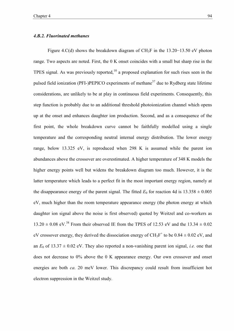
Chapter 4 94

4.B.2. Fluorinated methanes

Figure 4.C(d) shows the breakdown diagram of CH3F in the 13.20−13.50 eV photon

range. Two aspects are noted. First, the 0 K onset coincides with a small but sharp rise in the

TPES signal. As was previously reported,10 a proposed explanation for such rises seen in the

pulsed field ionization (PFI-)PEPICO experiments of methane37 due to Rydberg state lifetime

considerations, are unlikely to be at play in continuous field experiments. Consequently, this

step function is probably due to an additional threshold photoionization channel which opens

up at the onset and enhances daughter ion production. Second, and as a consequence of the

first point, the whole breakdown curve cannot be faithfully modelled using a single

temperature and the corresponding neutral internal energy distribution. The lower energy

range, below 13.325 eV, is reproduced when 298 K is assumed while the parent ion

abundances above the crossover are overestimated. A higher temperature of 348 K models the

higher energy points well but widens the breakdown diagram too much. However, it is the

latter temperature which leads to a perfect fit in the most important energy region, namely at

the disappearance energy of the parent signal. The fitted E0 for reaction 4d is 13.358 ± 0.005

eV, much higher than the room temperature appearance energy (the photon energy at which

daughter ion signal above the noise is first observed) quoted by Weitzel and co-workers as

13.20 ± 0.08 eV.38 From their observed IE from the TPES of 12.53 eV and the 13.34 ± 0.02

eV crossover energy, they derived the dissociation energy of CH3F+ to be 0.84 ± 0.02 eV, and

an E0 of 13.37 ± 0.02 eV. They also reported a non-vanishing parent ion signal, i.e. one that

does not decrease to 0% above the 0 K appearance energy. Our own crossover and onset

energies are both ca. 20 meV lower. This discrepancy could result from insufficient hot

electron suppression in the Weitzel study.

Chapter 4 95

The breakdown diagram of CH2F2 in the 12.85–13.20 eV photon energy range is

presented in Figure 4.C(e). The fitted E0 of reaction 3e is 13.060 ± 0.015 eV, with the larger

error limit being a result of the curve having a small gradient near the E0. This produces a

tailing off of the parent signal, instead of a sharp cut-off. A possible reason for this and the

slightly inferior signal-to-noise ratio at the onset energy compared with other molecules in

this study may lie with the subtraction of the hot electron contamination. If the threshold

electron yield is low at onset or changes quickly with photon energy, the ring area around the

detector (which is subtracted from the centre area signal) can be a poor representation of the

hot electron background in the centre. While the E0 is independent of sample temperature, the

shape of the curve at the onset is governed by it, and a softly-landing parent ion curve leads to

a less well defined E0. Using pulsed-field-ionization zero kinetic energy electrons (PFI-

ZEKE), Forysinski et al. found the 0 K H-loss appearance energy to be 13.065 ± 0.003 eV.39

This value from their laser-based very high resolution study is 5 meV higher than our own

reported value, but the two values are within the error limits. Both values are somewhat lower

than the appearance energy of CHF2+ at 298 K of 13.08 ± 0.03 eV reported by Seccombe et

al. from a lower resolution TPEPICO study.40

4.B.3. CBrClF2 and CHClF2

The breakdown diagram of CBrClF2 in the 11.15–11.50 eV photon energy range along

with the TPES is presented in Figure 4.C(f). The C–Br bond is the weakest, and therefore the

first dissociative photoionization channel produces CClF2+ + Br + eThe fitted E0 value is

11.342 ± 0.003 eV. There is some ambiguity as to the adiabatic IE for CBrClF2. The TPES

has been studied several times, and vertical ionization energies of 11.5141 and 11.83 eV42

Chapter 4 96

were reported. Another value for the IE is reported to be 11.21 eV, corresponding to the onset

of the electron signal.43 However, as can be seen from the TPES, the identification of the

adiabatic IE is not immediately obvious. Similarly to CHCl3 and CHClF2, there is a

significant daughter ion contribution of ca. 30 % at the ionization onset. The modelled

breakdown curve deviates from the experimental data points at a slightly higher energy of

11.23 ± 0.03 eV. We propose this somewhat higher value as the adiabatic IE of CBrClF2. This

fit is less sensitive to the assumed IE than for CHCl3 and CHClF2, as the deep well model

only deviates at most over a few tens of meV from the shallow well reality.

The breakdown diagram of CHClF2 (Figure 4.D), is shown in the 12.15–12.51 eV

photon energy range, plotted together with the corresponding TPES. The CCl bond is the

weakest, and the derived E0 value for reaction 4g, production of CHF2+, is 12.406 ± 0.004 eV.

This is the same daughter ion as the first product from CH2F2. As with CHCl3, there is

significant daughter ion abundance present in the low energy region of the breakdown

diagram, and the deep well approximation deviates from the experimental points over the

range of 12.2–12.3 eV. This provides us with an accurate IE of 12.30 ± 0.02 eV, which is not

easily determined from the TPES alone. The most recent ionization energies range from 12.15

± 0.05 eV determined by TPES,22 to 12.28 ± 0.02 eV determined by PIMS,43 so our value is at

the higher end of this range. Upon magnification, a small hump or bulge in the otherwise

smooth breakdown curve becomes apparent at 12.37 eV. Interestingly, this feature is also

faithfully reproduced by the model curves. To shed light on this peculiarity, we also plotted

the calculated neutral thermal energy distribution in Figure 4.D, with its origin shifted to

12.37 eV. Two possible reasons have been suggested for such features in breakdown

diagrams, namely alternative photoionization mechanisms10 or a less than faithful

transposition of the neutral thermal energy distribution to the ion manifold.1 Here, however,

Chapter 4 97

the explanation appears to be that the thermal energy distribution is indeed transposed onto

the ion manifold, and we use our molecular thermometer to measure the Boltzmann

distribution of neutral energies, which shows a dip at an internal energy of ca. 50 meV due to

the higher density of rovibrational levels 15 meV higher.

Figure 4.D. Breakdown diagram corresponding to Cl loss in the shallow well parent ion CHClF2+,

along with the new IE of 12.30 ± 0.02 eV. The ionization energy is hard to predict based on the broad featureless TPES shown in grey (inset). The inset also shows breakdown diagram modelled with the new IE, where the lower hν range is reproduced well by taking the actual potential energy well depth into account. The ion internal energy distribution at 12.37 eV is shown with parent contribution in grey and CClF2

+ contribution in pale blue. The hump in the breakdown curve, indicated by a double-headed arrow at 12.37 eV, corresponds to an unusual minimum in the thermal energy distribution in the neutral, confirming the faithful transposition of internal energy distribution upon threshold photoionization.

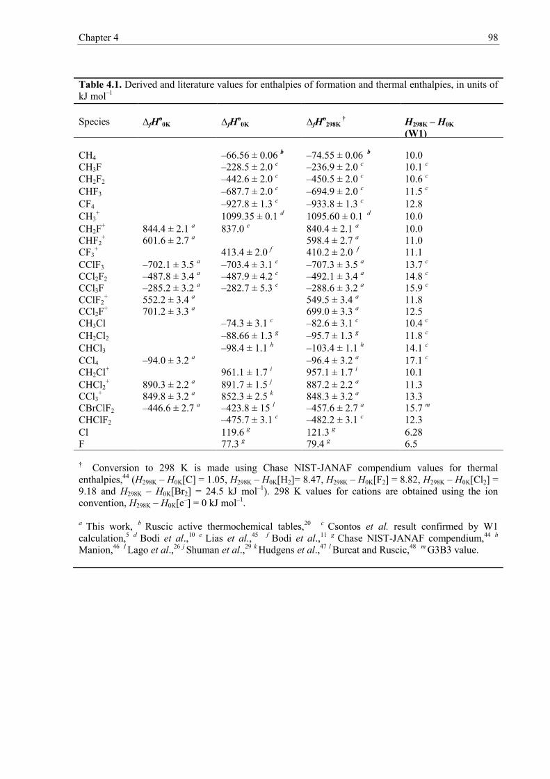
Chapter 4 98

Table 4.1. Derived and literature values for enthalpies of formation and thermal enthalpies, in units of kJ mol–1 Species

∆fHo

0K ∆fHo

0K ∆fHo

298K †

H298K – H0K (W1)

CH4

–66.56 ± 0.06 b –74.55 ± 0.06 b

10.0

CH3F –228.5 ± 2.0 c –236.9 ± 2.0 c 10.1 c

CH2F2 –442.6 ± 2.0 c –450.5 ± 2.0 c 10.6 c

CHF3 –687.7 ± 2.0 c –694.9 ± 2.0 c 11.5 c

CF4 –927.8 ± 1.3 c –933.8 ± 1.3 c 12.8 CH3

+ 1099.35 ± 0.1 d 1095.60 ± 0.1 d 10.0 CH2F+ 844.4 ± 2.1 a 837.0 e 840.4 ± 2.1 a 10.0 CHF2

+ 601.6 ± 2.7 a 598.4 ± 2.7 a 11.0 CF3

+ 413.4 ± 2.0 f 410.2 ± 2.0 f 11.1 CClF3 –702.1 ± 3.5 a –703.4 ± 3.1 c –707.3 ± 3.5 a 13.7 c

CCl2F2 –487.8 ± 3.4 a –487.9 ± 4.2 c –492.1 ± 3.4 a 14.8 c

CCl3F –285.2 ± 3.2 a –282.7 ± 5.3 c –288.6 ± 3.2 a 15.9 c

CClF2+ 552.2 ± 3.4 a 549.5 ± 3.4 a 11.8

CCl2F+ 701.2 ± 3.3 a 699.0 ± 3.3 a 12.5 CH3Cl –74.3 ± 3.1 c –82.6 ± 3.1 c 10.4 c

CH2Cl2 –88.66 ± 1.3 g –95.7 ± 1.3 g 11.8 c

CHCl3 –98.4 ± 1.1 h –103.4 ± 1.1 h 14.1 c

CCl4 –94.0 ± 3.2 a –96.4 ± 3.2 a 17.1 c

CH2Cl+ 961.1 ± 1.7 i 957.1 ± 1.7 i 10.1 CHCl2

+ 890.3 ± 2.2 a 891.7 ± 1.5 j 887.2 ± 2.2 a 11.3 CCl3

+ 849.8 ± 3.2 a 852.3 ± 2.5 k 848.3 ± 3.2 a 13.3 CBrClF2 –446.6 ± 2.7 a –423.8 ± 15 l –457.6 ± 2.7 a 15.7 m

CHClF2 –475.7 ± 3.1 c –482.2 ± 3.1 c 12.3 Cl 119.6 g 121.3 g 6.28 F 77.3 g 79.4 g 6.5

† Conversion to 298 K is made using Chase NIST-JANAF compendium values for thermal enthalpies,44 (H298K – H0K[C] = 1.05, H298K – H0K[H2]= 8.47, H298K – H0K[F2] = 8.82, H298K – H0K[Cl2] = 9.18 and H298K – H0K[Br2] = 24.5 kJ mol–1). 298 K values for cations are obtained using the ion convention, H298K – H0K[e–] = 0 kJ mol–1. a This work, b Ruscic active thermochemical tables,20 c Csontos et al. result confirmed by W1 calculation,5 d Bodi et al.,10 e Lias et al.,45 f Bodi et al.,11 g Chase NIST-JANAF compendium,44 h

Manion,46 I Lago et al.,26 j Shuman et al.,29 k Hudgens et al.,47 l Burcat and Ruscic,48 m G3B3 value.

Chapter 4 99

4.B.4. Thermochemistry

In addition to the measured 0 K appearance energies, the neutral parents and daughter

ions can be related to each other through a series of quantum chemical calculations involving

closed shell species, as well, to generate a network shown in Figure 4.E. The neutral network

is composed of three sub-networks, that of the chlorinated methanes, the fluorinated methanes

and the chlorofluoromethanes. Even though the accurate onset energy of CCl4, CF4 and CHF3

cannot be determined experimentally because they photoionize dissociatively, their neutral

enthalpies of formation feature in the network through computed reaction energies. Two

stand-alone compounds, CHClF2 and CBrClF2, are also studied, which only connect to the

rest of the network via their E0 values and as well as a neutral isodesmic reaction energy for

the former. Each sub-network contains the independent isodesmic reactions connecting the

neutrals, e.g. CHnX4–n, as well as the ions, e.g. CHnX3–n+, (X = F, Cl),

CHnX4–n + CHn–2X6–n → 2 CHn–1X5–n (n = 2–4) (4h)

CHnX3–n+ + CHn–2X5–n

+ → 2 CHn–1X4–n+ (n = 2, 3) (4i)

and the interconnecting exchange reactions for the ionic fragments where a new halomethane

is generated by the substitution of a hydrogen with a halogen (e.g. H2/X2),

CHnX3–n+ + ½X2 → CHn–1X4–n

+ + ½H2 (n = 1–3) (4j)

This approach was also adopted for the chlorofluoromethanes: CClnF4–n and CCln–1F4–n+. The

enthalpies of formation derived in this work are given in Table 4.1.

Chapter 4 100

Figure 4.E. The thermochemical network showing the experimental (E0) and computational links. Enthalpies of formation are indicated as nodes. The appearance energies (straight dashed arrows) connect the neutrals with the ions, ab initio isodesmic (pairs of black curved links), H2/(F2 or Cl2) and F2/Cl2 exchange reactions (double headed arrows) connect neutral/neutral, and ion/ion groups. Revised thermochemical values are indicated by dashed boxes. The absolute values of ∆fHo

0K are tethered to five anchor points: CH4, CF4, CHCl3, CH3

+ and CF3+.

In isodesmic reactions, the products and reactants have equal number of the same

types of bonds.49,50 It has been shown that these reactions yield reliable reaction energies,

especially for closed shell species.50,51 Quantum chemical calculations such as the composite

calculations used in this chapter often suffer from error accumulation arising from; basis set

truncation, inaccuracies calculating valence electron correlation and zero-point vibrational

energies,52 and in heavier atoms, difficulty with accurate recovery of spin–orbit coupling

effects.6,9 These errors as well as relativistic and core correlation effects are effectively

cancelled out in isodesmic reaction energy calculations.49,50

The network is essentially a graph of vertices (enthalpies of formation of ions and

neutrals) connected by edges. There are three types of edges; E0 onset energies, neutral and

ion isodesmic reaction energies, and exchange reaction energies (the latter only for fragment

Chapter 4 101

ions). The E0 onset energies interconnect the neutral and ion groups, whereas the isodesmic

and exchange reaction energies establish connections within the neutral and ion groups. If

available, isodesmic reaction energies were obtained based on the energy values reported by

Csontos et al.5 Otherwise, W1 calculated reaction energies were used. G3B3 results were also

obtained and checked for consistency, see Table 4.2 (please also see Appendix I). As a starting

point in the optimization of the enthalpies of formation, the isodesmic, exchange and

dissociative photoionization reaction energies were also calculated using the literature ∆fHo0K

values.

The entire network needs to be tethered to an absolute scale of enthalpies of formation,

and well-defined enthalpies of formation for a chosen set of species provide this vital link.

These ‘anchor’ enthalpies of formation are kept unchanged during the fitting process: ∆fHo0K

(CH4) = –66.56 ± 0.06,53 ∆fHo0K (CF4) = –927.8 ± 1.3,5,53 ∆fHo

0K (CF3+) = 413.4 ± 2.0,11 and

∆fHo0K (CHCl3) = –98.4 ± 1.1 kJ mol–1.46 The enthalpy of formation for CH3

+ is derived from

the 0 K onset energy for CH4 + hν → CH3+ + H + e– , 14.323 ± 0.001 eV27 combined with the

H atom heat of formation, which yield ∆fHo0K(CH3

+) = 1099.35 ± 0.1 kJ mol–1, yet another

anchor value. The two major groups of neutrals, the fluorinated methanes and chlorinated

methanes are ‘anchored’ by CF4/CH4 and CHCl3/CH4, respectively. The chlorofluoromethane

groups, CClnF4–n and CCln–1F4–n+, provide bridges between the chlorinated and the fluorinated

methanes.

An overall error function, (ε) is defined as the sum of component isodesmic, exchange

and experimental errors:

∑

( ) ∑

( ) ∑

( ) (3.3)

Chapter 4 102

where ( ) = (∆rHo[calc]iso – ∆rHo[∆fHo]iso)2, ( ) = (∆rHo[calc]exc –∆rHo[∆fHo]exc)2 and

( ) = (∆rHo[meas]iPEPICO–∆rHo[∆fHo]dissoc.photoionization)2. ∆rHo[calc] are the reaction

enthalpies at 0 K from ab intio calculations, and ∆rHo[∆fHo] are the enthalpy of formation

based reaction enthalpies, the starting values for which are taken from the literature. The

network is optimized by minimizing this error function using the Generalized Reduced

Gradient Method.54

Initially, the network is relaxed and all enthalpies of formation except the anchor

values are set as fit parameters. The exchange reaction error function is then weighted by 0.01

to make sure it influences the fit less than the isodesmic reaction errors, as the latter are more

reliable. There are fewer experimental onset energies, which are also more accurate than the

calculations. Therefore, the PEPICO error function is weighted by 100 to ensure its adequate

representation in the optimization of the network, (see Table 1.2, 1.3, 1.4 and 1.5 of Appendix

1). Thus, no data set over-influences the outcomes. Next, by analysing the optimized

enthalpies of formation in the fully relaxed fit, we identified further literature values which

could be kept constant in the fitting procedure. Notably, the enthalpies of formation reported

by Csontos et al.5 were compared with the optimized values. The average difference was

found to be 0.05 kJ mol–1, with a standard deviation of 0.77 kJ mol–1 and maximum of 1.35 kJ

mol–1 for CH3Cl, CH3F, CH2F2, CHF3, and CHClF2.5 These enthalpies of formation are, thus,

confirmed as recommended by Csontos et al. and held constant in the final fit. Furthermore,

the Chase value for ∆fHo0K (CH2Cl2) = –88.66 ± 1.3 kJ mol–1 and the Lago value for ∆fHo

0K

(CH2Cl+) = –961.1 ± 1.7 kJ mol–1 are kept unchanged.26,44 The remaining enthalpies of

formation for CH2F+, CHF2+, CClF2

+, CCl2F+, CHCl2+, CCl3

+, CF3Cl, CF2Cl2, CFCl3,

CBrClF2 and CCl4 are the final fit parameters. The network is anchored to CF4 on the left

hand side in Figure 4.E, but, since CCl4 is a fit parameter, an alternative, asymmetric anchor is

Chapter 4 103

required for the chloromethane series. As the Manion value for ∆rHo0K (CHCl3),46 –98.4 ± 1.1

kJ mol–1, has been used previously as an anchor value by Shuman et al.,29 and has a lower

error bar than the Csontos value of –94.6 ± 5.3 kJ mol–1, we have also opted for it to act as

anchor. Having established the anchor values, confirmed the most reliable literature enthalpies

of formation which are also kept unchanged, and set the error function weights to construct a

balanced fit, a final optimization was carried out to obtain the final results as summarized in

Table 4.1.

Three sources determine the uncertainties of the final results: (1) the uncertainties in

the anchor values which peg the network to the enthalpy of formation scale; (2) the

calculation errors; and (3) the errors in the iPEPICO appearance energies. These were

accounted for as follows: (1) the anchor values were set to the high and low limit of their

confidence interval, and a relaxed fit was carried out establishing the network confidence

interval for each optimized species; (2) a ± 2 kJ mol–1 uncertainty contribution was assumed

for calculations; (3) a further ± 2 kJ mol–1 uncertainty contribution was assumed for species,

on which we have no direct experimental appearance energy data; (4) the iPEPICO

appearance energy uncertainty was used otherwise. The confidence intervals listed in Table

4.1 are the result of these four contributions.

The conversion from 0 K to 298 K is made by the relationship:44

[ ] [ ] (4.4)

The list of thermal enthalpies, H298K – H0K, is shown in Table 4.1. The W1 values are virtually

identical to those from the Csontos et al. study.5 The latter are used for the neutral molecules

when available, but the G3B3 value is used for CBrClF2. W1 values are used for the

remaining neutrals and the fragment cations.

Chapter 4 104

First, we consider data for the chlorinated and fluorinated methanes. The 0 K enthalpy

of formation of CCl3+ is connected to the enthalpies of formation of CH2Cl+ and CHCl2

+ via

isodesmic and exchange pathways. Using well-established values for ∆fHo0K(CHCl3) = –98.4

± 1.1 kJ mol–1, 46 and ∆fHo0K (CH2Cl2) = –±kJ mol–1,44 our global fit derives revised

values for ∆fHo0K(CHCl2

+) = 890.3 ± 2.2 and ∆fHo0K(CCl3

+) = 849.8 ± 3.2 kJ mol–1. The

CHCl2+ value is similar to that determined by Shuman et al., 891.7 ± 1.5 kJ mol–1.29 The

revised ∆fHo0K(CCl3

+) value is about 15 kJ mol–1 higher than the 834.6 kJ mol–1 quoted by

Lias,45 and an earlier value of Rodriguez and co-workers of 831.6 kJ mol–1.55 However it

agrees with the Robles et al. value of 847.68 ± 3.3 kJ mol–1 derived from ∆fHo0K(CCl3) = 69.8

± 2.5 kJ mol–1 and their measured IE(CCl3) = 8.06 ± 0.02 eV.56 It is also within the error limit

of the Hudgens et al. value of ∆fHo0K(CCl3

+) = 852.3 ± 2.5 kJ mol–1, also derived from

photoionization of CCl3.47

CH2F+ and CHF2+ are fitted parameters. They connect in the network to the fixed

values of ∆fHo0K of CH3F, CH2F2 and CHClF2 via their experimental 0 K appearance energies.

We note that an experimental value for the enthalpy of formation of CH3F has been

surprisingly hard to determine, with Chase et al. quoting a value of 226 ± 33 kJ mol–1.44 One

year earlier, Luo and Benson had recommended the ‘best’ experimental value at 298 K to be

233.9 ± 4.2 kJ mol–1, corresponding to 225.5 ± 4.2 kJ mol–1 at 0 K.57 Given the importance

and relative simplicity of this five-atom halogenated hydrocarbon, it is perhaps surprising that

the range of theoretical values in the literature is also large. Values at 0 K from 224 to 230

kJ mol–1 have been reported by many authors, with errors spanning from ± 0.8 to ± 10.0 kJ

mol–1.5,18,48,58-60 As explained above, we have fixed the 0 K value for CH3F to that determined

by Csontos et al., 228.5 ± 2.0 kJ mol–1.5 By contrast, the Chase and Csontos values for

CH2F2 are almost equal, with similar errors of ca. ± 2.0 kJ mol–1. The heat of formation of

Chapter 4 105

CHClF2 is reported by Csontos et al. to be –475.7 ± 3.1 kJ mol–1,5 with no obvious

experimental value for comparison. The new value for ∆fHo0K(CH2F+) of 844.4 ± 2.1 kJ mol–1

is significantly higher than that reported by Lias et al., 837.0 kJ mol–1.45 The new value for

∆fHo0K(CHF2

+), 601.6 ± 2.7 kJ mol–1, is equivalent to 598.4 ± 2.7 kJ mol–1 at 298 K. This

latter value is in reasonable agreement with a recent experimental value at 298 K from

Seccombe et al. of 604 ± 3 kJ mol–1,40,61 where the appearance energy at this temperature of

CHF2+ from CH2F2 was corrected for thermal effects by the procedure of Traeger et al.62

The experimental route is important here because reliable quantum chemical

calculations involving bromine containing compounds are difficult to perform59 due to the

large numbers of electrons, and the fact that relativistic effects become significant for high–Z

atoms.18,63,64 Although Borkar et al. have found that relative energies of C3H5Br isomers can

be quite well predicted by standard computational methods,65 bromine and iodine containing

species are omitted in the comprehensive study of Csontos et al.,5 and Bodi et al. report large

error bars, typically in the region of 7 kJ mol–1 in a recent study on bromofluoromthanes.11

The study of CBrClF2 provides a link between bromine containing species and the remainder

of the lighter Cl and F containing species. Little is known about the enthalpy of formation of

CBrClF2, indeed the only value we could find was –423.8 ± 15 kJ mol–1 given by Burcat.48 As

such, the heat of formation becomes a ‘fit’ parameter, which is only connected to the network

by the E0 of the reaction CBrClF2 → CClF2+ + Br + e–. Barring an overall reverse barrier, the

result, ∆fHo0K(CBrClF2) = –446.6 ± 2.7 kJ mol–1, falls just outside the generous error limit of

the previous value.

The enthalpy of formation of CCl4 given by Csontos et al. of –88.7 ± 6.4 kJ mol–1 lies

toward the less negative end of the literature values and has the largest error limit among the

values they derived.5 We derive a revised more negative value for ∆fHo0K of –94.0 ± 3.2 kJ

Chapter 4 106

mol–1. This value is in excellent agreement to the Rodgers et al.66 value of –93.7 ± 0.6 kJ mol–

1 and the Chase value of –93.8 ± 2.1 kJ mol–1.44 We note that Csontos et al. seem to report

more reliable enthalpies of formation for fluorine substituted methanes such as CHF3, than

when methane is substituted with multiple chlorine atoms such as in CHCl3 and CCl4.

Due to the lack of certainty regarding the enthalpies of formation of CCl3F, CCl2F2

and CClF3 in the literature, these values were also fitted. The resulting enthalpies are;

∆fHo0K(CCl3F) = –285.2 ± 3.2, ∆fHo

0K(CCl2F2) = –487.8 ± 3.4 and ∆fHo0K (CClF3) = –702.1 ±

3.5 kJ mol–1. These values are within the uncertainty limits of the Csontos et al. values,

namely, –282.7 ± 5.3, –487.9 ± 4.2 and –703.4 ± 3.1 kJ mol–1, respectively.5 The Chase

values of ∆fHo0K(CCl3F) = –285.5 ± 6.3 kJ mol–1 and ∆fHo

0K(CClF3) = –702.8 ± 3.3 kJ mol–1

are also in close agreement with our results.44 Whilst there are no experimental results leading

directly to CCl2F+ or CClF2+ in this work, their 0 K enthalpies of formation have been

determined by isodesmic and exchange reaction energies to be 701.2 ± 3.3 and 552.2 ± 3.4 kJ

mol–1, respectively.

Chapter 4 107

Table 4.2. Enthalpies of reaction used for the thermochemical network in this chapter. Column (h) is included as an example of the difference between enthalpies of reaction determined using the average of the calculated enthalpies of reaction (f) and enthalpies of reaction determined using literature values of the enthalpies of formation of the constituent molecules. Column (h) varies with each iteration of the global fit to minimize the sum of errors (sum of column (h)).

(a) (b) (c) (d) (e) (f) (g) (h)

Reaction G3B3 0K ∆rH

o(eV)

CBS-QB3 0K ∆rH

o(eV)

W1 0K ∆rH

o(eV) E0(eV)

CSONTOS (eV)

W1 values or Csontos values where avaliable ∆rH

o (eV)

From [litetature ∆fH

o ] ∆rH

o

eV ERROR (f)-(g)

first onsets CHCl3 → CHCl2

+ + Cl 11.497 11.545 11.542 11.487

11.487 11.495 9.70E-08

CH2Cl2 → CH2Cl+ + Cl 12.098 12.130 12.163 12.108

12.108 12.120 1.34E-02

CH3Cl → CH2Cl+ + H 12.935 12.962 13.020 12.981

12.981 12.970 1.17E-04

Isodesmic reactions CCl3

+ + CH2Cl+ → 2CHCl2+ -0.291 -0.291 -0.312

-0.312 -0.139 6.88E-07

CHCl2+ + CH3

+ → 2 CH2Cl+ -0.724 -0.707 -0.701

-0.701 -0.707 2.09E-06

CCl4 + CH2Cl2 → 2CHCl3 -0.093 -0.099 -0.136

-0.146 -0.141 -0.200 8.52E-23

CHCl3 + CH3Cl → 2CH2Cl2 -0.020 -0.023 -0.055

-0.042 -0.049 -0.052 3.26E-05

CH2Cl2 + CH4 → 2CH3Cl 0.069 0.067 0.034

0.034 0.071 1.18E-03

exchange reactions CCl3

+ +1/2H2 → CHCl2+ + 1/2Cl2 -0.546 -0.563 -0.604

-0.604 -0.414 6.18E-06

CHCl2+ +1/2H2 → CH2Cl+ +

1/2Cl2 -0.255 -0.272 -0.292

-0.292 -0.274 6.60E-06

CH2Cl+ +1/2H2 → CH3+ + 1/2Cl2 0.469 0.435 0.409

0.409 0.433 5.87E-06

Chapter 4 108

(a) (b) (c) (d) (e) (f) (g) (h)

first onsets CH3F → CH2F

+ + H 13.364 13.370 13.370 13.358

13.358 13.277 2.53E-05

CH2F2 → CHF2+ + H 13.085 13.062 13.077 13.055

13.055 13.217 1.29E-04

Isodesmic reactions CF3

+ + CH2F+ → 2CHF2

+ -0.555 -0.555 -0.559

-0.559 -0.173 5.43E-05

CHF2 + + CH3

+ → 2CH2F+ -0.107 -0.105 -0.098

-0.098 -0.445 8.24E-04

CF4 + CH2F2 → 2CHF3 -0.088 -0.078 -0.089

-0.053 -0.053 -0.052 8.36E-07

CHF3 + CH3F → 2CH2F2 0.310 0.328 0.318

0.322 0.322 0.322 4.10E-07

CH2F2 + CH4 → 2CH3F 0.558 0.576 0.561

n/a 0.561 0.541 4.21E-04

exchange reactions CF3

+ +1/2H2 → CHF2+ + 1/2F2 0.550 0.560 0.560

0.560 0.512 2.27E-05

CHF2+ +1/2H2 → CH2F

+ + 1/2F2 1.106 1.115 1.119

1.119 1.078 1.62E-05

CH2F+ +1/2H2 → CH3

+ + 1/2F2 1.212 1.220 1.216

1.216 1.205 1.34E-06

first onsets CF3Cl → CF3

+ + Cl 12.861 n/a 12.823 12.801

12.801 12.801 1.58E-05

CF2Cl2 → CClF2+ + Cl 12.079 n/a 12.068 12.03

12.03 12.01 7.96E-02

Isodesmic reactions CF3

+ + CCl2F+ → 2CClF2

+ -0.124

-0.107

-0.107 -0.107 5.76E-17

CCl3+ + CClF2

+ → 2CCl2F+ -0.003

0.005

0.005 0.005 4.16E-17

CF4 + CCl2F2 → 2CF3Cl 0.091

0.091

0.091 0.091 0.118 7.00E-04

CClF3 + CFCl3 →2 CF2Cl2 0.103

0.103

0.108 0.108 0.121 1.75E-04

Chapter 4 109

(a) (b) (c) (d) (e) (f) (g) (h)

CF4 + CHCl3 → CCl3F + CHF3 0.457

0.539 0.539 0.552 1.75E-04

exchange reactions CF3

+ +1/2Cl2 → CF2Cl+ + 1/2F2 0.983

1.058

1.058 0.999 3.38E-05

CF2Cl+ +1/2Cl2 → CFCl2+ + 1/2F2 1.107

1.164

1.164 1.106 3.38E-05

CFCl2+ +1/2Cl2 → CCl3

+ + 1/2F2 1.110

1.160

1.160 1.102 3.38E-05

first onsets CHClF2 → CHF2

+ + Cl 12.448

12.435 12.406

12.406 12.404 1.63E-04

CHCl2F → CHFCl+ + Cl 12.945 13.019 11.909 Not included

Isodesmic reactions

CF4 + CH2Cl2 → 2CHClF2 0.622

0.644

0.652 0.652 0.674 4.89E-04

first onsets CBrClF2 → CClF2

+ + Br 11.401

11.342

11.342 11.342 2.98E-16

Chapter 4 110

4.C. Conclusions

The thermochemistry of the halogenated methanes CH3Cl, CH2Cl2, CHCl3, CH3F,

CH2F2, CHClF2 and CBrClF2, and their fragment ions CH2Cl+, CHCl2+, CCl3

+, CH2F+,

CHF2+, CCl2F+ and CClF2

+ was studied using a combination of experimental data from

imaging photoelectron photoion coincidence spectroscopy and ab initio calculations of

isodesmic and exchange reaction energies. A thermochemical network was constructed, in

which the neutral and ionic components were intra-connected by sub-networks of isodesmic

and exchange reactions, and interconnected by the experimental 0 K dissociative

photoionization energies. The network was anchored by the well–known enthalpies of

formation for CF4, CH4, CHCl3, CF3+ and CH3

+. An error function was defined between

measured dissociative photoionization onsets and calculated reaction energies on the one

hand, and the reaction energies derived using the enthalpies of formation in the network

vertices on the other. The optimum values for the enthalpies of formation were determined by

minimizing this error function. This holistic approach has been successful in producing

updated thermochemical values at 0 K for the neutrals CCl4, CBrClF2, CClF3, CCl2F2 and

CCl3F, as –94.0 ± 3.2, –446.6 ± 2.7, –702.1 ± 3.5, –487.8 ± 3.4 and –285.2 ± 3.2 kJ mol–1,

respectively. Fitting the remaining neutral enthalpies of formation led to negligible changes.

These selected values were held constant, and are therefore confirmed. Revised 0 K enthalpies

of formation for the ions CH2F+, CHF2+, CClF2

+, CCl2F+, CHCl2+ and CCl3

+ have been

determined as 844.4 ± 2.1, 601.6 ± 2.7, 552.2 ± 3.4, 701.2 ± 3.3, 890.3 ± 2.2 and 849.8 ± 3.2

kJ mol–1, respectively. The adiabatic IEs can easily be obtained based on the breakdown

diagram of weakly bound parent ions that only exist in a Franck–Condon allowed shallow

potential energy well. These have been found to be 11.47 ± 0.01 eV, 12.30 ± 0.02 eV and

11.23 ± 0.03 eV for CHCl3, CHClF2 and CBrClF2, respectively. We suggest that this is the

Chapter 4 111

experimental method of choice to determine the IE of molecules where the ground state of the

parent ion is only weakly bound. Finally, because of an uncharacteristic dip in the density of

states, the thermal energy distribution of CHClF2 shows a minimum at 50 meV. This

interesting feature is also seen and modelled as a small hump at 12.37 eV in the otherwise

smooth breakdown curve for CHClF2+.

Chapter 4 112

References

(1) Sztáray, B.; Bodi, A.; Baer, T. J. Mass Spectrom. 2010, 45, 1233-1245. (2) Gaussian 09, Revision A.1, Gaussian, Inc.: Wallingford CT, 2009. (3) Baboul, A. G.; Curtiss, L. A.; Redfern, P. C.; Raghavachari, K. J. J. Chem. Phys.

1999, 110, 7650-7657. (4) Martin, J. M. L.; de Oliveira, G. J. Chem. Phys. 1999, 111, 1843-1856. (5) Csontos, J.; Rolik, Z.; Das, S.; Kállay, M. J. Phys. Chem. A. 2010, 114, 13093. (6) Peterson, K. A.; Feller, D.; Dixon, D. A. Theor. Chem. Acc. 2012, 131, 1079-1099. (7) Karton, A.; Daon, S.; Martin, J. M. L. Chem. Phys. Letts. 2011, 510, 165-178. (8) Feller, D.; Peterson, K. A.; Dixon, D. A. J. Phys. Chem. A. 2011, 115, 1440-1451. (9) Feller, D.; Peterson, K. A.; Grant Hill, J. J. Chem. Phys. 2011, 135, 044102-044120. (10) Bodi, A.; Shuman, N. S.; Baer, T. Phys. Chem. Chem. Phys. 2009, 11, 11013-11021. (11) Bodi, A.; Kvaran, Á.; Sztáray, B. J. Phys. Chem. A. 2011, 115, 13443-13451. (12) Borkar, S.; Sztáray, B. J. Phys. Chem. A. 2010, 114, 6117-6123. (13) Boese, A. D.; Oren, M.; Atasoylu, O.; Martin, J. M. L.; Kállay, M.; Gauss, J. J. Chem.

Phys. 2004, 120, 4129-4142. (14) Tajti, A.; Szalay, P. G.; Császár, A. G.; Kállay, M.; Gauss, J.; Valeev, E. F.; Flowers,

B. A.; Vázquez, J.; Stanton, J. F. J. Chem. Phys. 2004, 121, 11599-11613. (15) Baer, T.; Sztáray, B.; Kercher, J. P.; Lago, A. F.; Bodi, A.; Skull, C.; Palathinkal, D.

Phys. Chem. Chem. Phys. 2005, 7, 1507-1513. (16) Kercher, J. P.; Stevens, W.; Gengeliczki, Z.; Baer, T. Int. J. Mass. Spectrom. 2007,

267 159-166. (17) Baer, T.; Walker, S. H.; Shuman, N. S.; Bodi, A. J. Phys. Chem. A. 2012, 116, 2833-

2844. (18) Lazarou, Y. G.; Papadimitriou, V. C.; Prosmitis, A. V.; Papagiannakopoulos, P. J.

Phys. Chem. A. 2002, 106, 11502-11517. (19) Simpson, M.; Tuckett, R. P. J. Phys. Chem. A. 2012, 116, 8119-8129. (20) Ruscic, B. Active Thermochemical Tables, early beta 1.110,

http://atct.anl.gov/index.html, May 09 2012. (21) Bodi, A.; Kercher, J. P.; Bond, C.; Meteesatien, P.; Sztáray, B.; Baer, T. J. Phys.

Chem. A. 2006, 110, 13425-13433. (22) Howle, C. R.; Collins, D. J.; Tuckett, R. P.; Malins, A. E. R. Phys. Chem. Chem. Phys.

2005, 7, 2287-2297. (23) Smith, D. M.; Tuckett, R. P.; Yoxall, K. R.; Codling, K.; Hatherly, P. A. Chem. Phys.

1993, 216, 493-502. (24) Simm, I. G.; Danby, C. J.; Eland, J. H. D.; Mansell, P. I. J. Chem. Soc., Faraday

Trans. 2 1976, 72, 426-434 (25) Parkes, M. A.; Chim, R. Y. L.; Mayhew, C. A.; Mikhailov, V. A.; Tuckett, R. P. Mol.

Phys. 2006, 104, 263-272. (26) Lago, A. F.; Kercher, J. P.; Bodi, A.; Sztáray, B.; Miller, B.; Wurzelmann, D.; Baer,

T. J. Phys. Chem. A. 2005, 109, 1802-1809. (27) Weitzel, K.-M.; Malow, M.; Jarvis, G. K.; Baer, T.; Song, Y.; Ng, C. Y. J. Chem.

Phys. 1999, 111, 8267-8270. (28) Song, Y.; Qian, X.-M.; Lau, K.-C.; Ng, C. Y.; Liu, J.; Chen, W. J. Chem. Phys. 2001,

115, 4095-4104. (29) Shuman, N.; Zhao, L. Y.; Boles, M.; Baer, T.; Sztáray, B. J. Phys. Chem. A. 2008,

112, 10533-10538. (30) Tang, X.; Zhou, X.; Wu, M.; Liu, S.; Liu, F.; Shan, X.; Sheng, L. J. Chem. Phys.

2012, 136, 034304-034312. (31) Lane, I. C.; Powis, I. J. Phys. Chem. 1993, 97, 5803-5808.

http://atct.anl.gov/index.html

Chapter 4 113

(32) Werner, A., S.; Tsai, B. P.; Baer, T. J. Chem. Phys. 1974, 60, 3650-3657. (33) Von Niessen, W.; Åsbrink, L.; Bieri, G. J. Electron Spectrosc. Relat. Phenom. 1982,

26, 173-201. (34) Schuman, N.; Zhao, L. Y.; Boles, M.; Baer, T.; Sztáray, B. J. Phys. Chem. A 2008,

112, 10533–10538. (35) Innocenti, F.; Eypper, M.; Lee, E. P. F.; Stranges, S.; Mok, D. K. W.; Chau, F.-t.;

King, G. C.; Dyke, J. M. Chem. Eur. J. 2008, 14, 11452-11460. (36) Seccombe, D. P.; Chim, R. Y. L.; Jarvis, G. K.; Tuckett, R. P. Phys. Chem. Chem.

Phys. 2000, 2, 769-780. (37) Weitzel, K.-M.; Jarvis, G. K.; Malow, M.; Baer, T.; Song, Y.; Ng, C. Y. Phys. Rev.

Lett 2001, 86, 3526-3529. (38) Weitzel, K.-M.; Güthe, F.; Mähnert, J.; Locht, R.; Baumgärtel, H. Chem. Phys. 1995,

201, 287-298. (39) Forysinski, P. W.; Zielke, P.; Luckhaus, D.; Signorell, R. Phys. Chem. Chem. Phys.

2010, 12, 3121-3130. (40) Seccombe, D. P.; Tuckett, R. P.; Fisher, B. O. J. Chem. Phys. 2001, 114, 4074-4088. (41) Cvitaš, T.; Klasinc, L.; Novak, I. Int. J. Quantum Chem. 1980, 18, 305-313. (42) Douct, J.; Gilbert, R.; Sauvageau, P.; Sandorfy, C. J. Chem. Phys. 1975, 62, 366-369. (43) Lias, S. G.; Bartmess, J. E.; Liebman, J. F.; Holmes, J. L.; Levin, R. D.; Mallard, W.

G. "Ion Energetics Data". In NIST Chemistry WebBook, NIST Standard Reference Database Number 69; Linstrom, P. J., Mallard, W. G., Eds.; National Institute of Standards and Technology, Gaithersburg MD, 20899.

(44) Chase, M. W. J. Phys. Chem. Ref. Data., Monograph 9. 1998. (45) Lias, S. G.; Bartmess, J. E.; Liebman, J. F.; Holmes, J. L.; Levin, R. D.; Mallard, W.

G. J. Phys. Chem. Ref. Data. 1988, 17. (46) Manion, J. A. J. Phys. Chem. Ref. Data. 2002, 31, 124-165. (47) Hudgens, J. W.; Johnson, R. D. I.; Timonen, R. S.; Seetula, J. A.; Gutman, D. J. Phys.

Chem. 1991, 95, 4400-4405. (48) Burcat, A.; Ruscic, B.September 2005 Third Millennium Ideal Gas and Condensed

Phase Thermochemical Database for Combustion with Updates from Active Thermochemical Tables, ANL-05/20 and TAE 960, Technion-IIT; Aerospace Engineering, and Argonne National Laboratory, Chemistry Division.September 2011.ftp://ftp.technion.ac.il/pub/supported/aetdd/thermodynamics.

(49) Wheeler, S. E.; Houk, v.; Schleyer, P. v. R.; Allen, W. D. J. Am. Chem. Soc. 2009, 131, 2547-2560.

(50) Wodrich, M. D.; Corminboeuf, C.; Wheeler, S. E. J. Phys. Chem. A. 2012, 116, 3436-3447.

(51) Raghavachari, K.; Stefanov, B. B.; Curtiss, L. A. J. Chem. Phys. 1997, 106, 6764-6767.

(52) Feller, D.; Peterson, K. A.; Dixon, D. A. J. Chem. Phys. 2008, 129, 204105-204136. (53) Ruscic, B. Active Thermochemical Tables, early beta 1.110, 2012. (54) Lasdon, L. S.; Waren, A. D. Generalized Reduced Gradient -2 User’s guide (as

implemented in the Excell program); School of Business Administration, University of Texas at Austin, 1986.

(55) Rodriquez, C. F.; Bohme, D. K.; Hopkinson, A. C. J. Phys. Chem. 1996, 100, 2942-2949.

(56) Robles, E. S. J.; Chen, P. J. Phys. Chem. 1994, 98, 6919-6923. (57) Luo, Y. R.; Benson, S. W. J. Phys. Chem. A. 1997, 101, 3042-3044. (58) Berry, R. J.; Burgess, D. R. F.; Nyden, M. R.; Zachariah, M. R. J. Phys. Chem. A.

1995, 99, 17145-17150. (59) Feller, D.; Peterson, K. A.; Jong, W. A. d.; Dixon, D. A. J. Chem. Phys. 2003, 118,

3510-3522. (60) Kormos, B. L.; Liebman, J. F.; Cramer, C. J. J. Phys. Org. Chem. 2004, 17, 656-664.


Chapter 4 114

(61) Zhou, W.; Seccombe, D. P.; Tuckett, R. P.; Thomas, M. K. Chem. Phys. 2002, 283, 419-431.

(62) Traeger, J. C.; McLoughlin, R. G. J. Am. Chem. Soc. 1981, 103, 3647-3652. (63) Dixon, D. A.; Grant, D. J.; Christe, K. O.; Peterson, K. A. Inorg. Chem. 2008, 47,

5485-5494. (64) Grant, D. J.; Garner, E. B.; Matus, M. H.; Nguyen, M. T.; Peterson, K. A.; Francisco,

J. S.; Dixon, D. A. J. Phys. Chem. A. 2010, 114, 4254-4265. (65) Borkar, S. N.; Sztáray, B.; Bodi, A. Int. J. Mass Spectrom., Accepted. 2012. (66) Rodgers, A. S.; Chao, J.; Wilhoit, R. C.; Zwolinski, B. J. J. Phys. Chem. Ref. Data

1974, 3, 117-140.

Chapter 5 115

Chapter 5:

Photodissociation dynamics of four fluorinated

ethenes: fast, slow, statistical and non-statistical

reactions.

Preamble

The results presented in this chapter have been previously published as a journal

article entitled ‘Dissociation dynamics of fluorinated ethene cations: from time bombs on a

molecular level to double-regime dissociators’ by J. Harvey, A. Bodi, R. P. Tuckett and B.

Sztáray, in 2012 in the Royal Society of Chemistry journal, Physical Chemistry Chemical

Physics, volume 14, pages 3935-3948. The majority of the data collection and analysis was

performed by myself, however, the assistance lent by Ms Nicola Rogers, Drs Mathew

Simpson Andras Bodi, Melanie Johnson, and Professor Richard Tuckett during beamtime

with the collection of the data is gratefully acknowledged. The modelling program was

developed by B. Sztáray, A. Bodi and T. Baer.1

Chapter 5 116

5.A. Introduction

The study of the swift dissociation dynamics (k >107 s–1) of small systems, the

halogenated methanes dissociating into their first daughter ions, has been presented in

Chapter 4. It was found that to accurately locate the E0, inspection of the breakdown diagram

can be an inadequate method, and modelling the breakdown diagram is required. However for

such systems, only the internal energy distributions are necessary to model it. In this chapter,

attention is also given to the dynamics of slowly dissociating molecules (those on a timescale

of 103 s–1 < k <107 s–1). Furthermore, whilst only the appearance energy of the first product

daughter ion was measured in those studies within Chapter 4, parallel and sequential reaction

channels of the four fluorinated ethenes; C2H3F+, 1,1-C2H2F2+, C2HF3

+ and C2F4+ are now

explored.

The C–F bond is one of the strongest in organic molecules. Exceptions include the C–

H bond in acetylene, the C=C double and C≡C triple bonds.2 This makes fluorinated alkanes

and alkenes particularly appealing subjects in studies of their bonding, electronic

spectroscopy and dissociation properties, because the strong bonding also results in sparsely

spaced electronic levels. In addition, the small size of the fluorine atom makes these organic

compounds amenable to computational chemistry studies, in which thermochemical

properties such as enthalpies of formation can be determined.3 In contrast to saturated

perfluorocarbons,4 which photoionize dissociatively even at their ionization energy so that

parent ion signal is not detectable, the unsaturated fluorinated ethenes form stable molecular

ions.5 Partly because of this great stability, early studies of fluorinated ethene cations have

Chapter 5 117

shown they are metastable with respect to dissociation at low internal energies6 and can

exhibit isolated state behaviour.7,8

The dissociative photoionization of monofluoroethene and 1,1-difluoroethene was first

investigated using threshold coincidence techniques by Güthe et al.,9 who reported complete

kinetic energy release distributions (KERD) for the HF and F loss reaction channels based on

the time-of-flight (TOF) spectra of the daughter ions. However, the insufficient mass

resolution in the experiment did not allow for the determination of the appearance energy of

the F-loss product, C2H2F+, from 1,1-C2H2F2+. In a second paper, Güthe et al.10 further

explored the metastable nature of the parent ion in the lowest energy dissociation channel, i.e.

HF elimination from both C2H3F+ and 1,1-C2H2F2+. Lifetimes on the order of several μs were

found using both linear and reflectron time-of-flight mass spectrometers. They reported

dissociation rate constants for both ions over a range from threshold to 400 meV above

threshold, the smallest of which, 8•104 s–1, was observed with the linear TOF. A tight 4-

membered ring transition state with a calculated reverse barrier of 163 kJ mol–1 had been

suggested for HF loss from 1,1-C2H2F2+,11 in contrast with the smaller measured reverse

barrier of only 95 kJ mol–1. Analogously to HCl loss from C2H5Cl12 or H2 loss from C2H4,13

Güthe et al. proposed H atom tunnelling to explain this discrepancy. The bimodal behaviour,

composed of the statistical as well as the non-statistical dissociations, of F-loss from 1,1-

C2H2F2+ was investigated by Gridelet et al., by examination of the KERDs using the

maximum entropy method.14 Only the lower energy dissociative photoionization modus was

found to be a statistical adiabatic reaction from the ionic ground state of the parent molecule,

which formed a narrow KERD component.

Chapter 5 118

The dissociative photoionization dynamics of trifluoroethene have not previously been

studied. Tetrafluoroethene was the subject of a threshold coincidence study by Jarvis et al.5

They reported that F loss from C2F4+ is accompanied by high kinetic energy (KE) release, too

large to be justified by a purely impulsive model, and they suggested two explanations. First,

that the heat of formation used to determine the thermochemical threshold for C2F3+

production was too high, and dissociation occurs below 15.85 eV. Second, that C2F4+ may

decay via a ‘modified impulsive’ mechanism, where energy is deposited exclusively into the

rotational and translational modes.

In this chapter, the imaging photoelectron photoion coincidence (iPEPICO)

experiment15 at the VUV beamline16 of the Swiss Light Source (SLS) was used to prepare and

study the dissociation dynamics of internal energy selected ions of monofluoroethene, 1,1-

difluoroethene, trifluoroethene and tetrafluoroethene in the 13−20 eV photon energy range

with a resolution much higher than in previous studies, i.e. only a few meV. The residence

time of photoions in the acceleration region of the TOF mass spectrometer is several μs. If,

while the ion resides in the acceleration region, there is significant dissociation then the

fragment ion peak shapes are asymmetric and their analysis can yield dissociation rate

constants,17 which are measured in the 103 s–1 < k < 107 s–1 range. This effect is distinct and

different from a symmetrical TOF peak broadening due to kinetic energy release. The

iPEPICO experiment yields both the threshold photoelectron spectrum (TPES) as well as

parent and daughter ion fractional abundances as a function of the photon energy, which

translates into an ion internal energy scan when the ion signal is evaluated in coincidence with

threshold electrons. Metastable and parallel fragmentations can be modelled in the framework

Chapter 5 119

of the statistical theory of unimolecular reactions: the asymmetric TOF distributions yield the

rate curve, k(E), as a function of internal energy which can be extrapolated to the 0 K

appearance energy, E0, where k(E) vanishes. Accurate appearance energies of the daughter

ions at 0 K can thus be established even when the low reaction rates result in incomplete

dissociation of the parent ions, an effect often referred to as the kinetic shift.18 For fast

dissociations in small molecules, the disappearance energy of the energy-selected parent ion

signal yields the 0 K appearance energy, i.e. the energy at which all photoions, including

those formed from neutrals with zero internal energy, are above the threshold.19

What does this appearance energy mean? Most ionic dissociations consist of simple

bond breaking, which take place along purely attractive potential energy curves. In such

instances, the 0 K appearance energy equals the dissociative photoionization energy, Edp. This

Edp value can be used in thermochemical cycles to determine 0 K enthalpies of formation for

daughter ions, when the precursor parent enthalpy of formation is known, or vice versa, see

Figure 5.A(a).20 In reactions that involve rearrangements, such as HF-loss, the barrier in the

backward direction also has to be considered. Neglecting tunnelling, the appearance energy

and the dissociative photoionization energy together can yield the value of this backward or

reverse barrier, Erb in Figure 5.A(b). Please refer to Appendix II for all input parameters used

to model the breakdown curves.

Chapter 5 120

Figure 5.A. Energy diagram for the dissociations of (a) C2H3F+ into C2H3+ + F without and (b) C2H3F+

into C2H2+ + HF with a reverse barrier, IE is the ionization energy, Edp is the dissociative

photoionization energy, Erb is the height of the reverse barrier, E0 is the 0 K appearance energy at which the products are first energetically accessible in the absence of tunnelling, and E0 – IE is the height of the forward barrier. When there is no reverse barrier present, E0 = Edp.

A process is considered statistical if the complete phase space is accessible to the

system. The ion density of states is dominated by the ground electronic state of the parent

cation, which implies that the dissociation takes place from this ground electronic state. The

adiabatic ionization energies of monofluoroethene, 1,1-difluoroethene, trifluoroethene and

tetrafluoroethene are 10.37, 10.30, 10.1421 and 10.11 eV,22 respectively. The dissociative

photoionization channels all take place above 13 eV at energies corresponding to excited

valence states of the four parent cations or in Franck–Condon gaps. If decay processes from

Chapter 5 121

these excited states to the ground state are slower than other processes, such as fluorescence

or even dissociation, some excited states may have an isolated character and follow a non-

statistical path. This has been suggested for several halogen containing ions, such as C2F4,5

CF3I,23 SiCl4,24 as well as Sn(CH3)3Cl, Sn(CH3)3Br25 and even for CH3OH.26,27 There are

features uncharacteristic of statistical processes present in the breakdown diagrams of all four

fluorinated ethene ions studied in this thesis. Most notably, the fractional abundance of the

daughter ions arising from F loss often follows the band intensities of the TPE spectrum of the

neutral molecule.

Two intriguing aspects of the dissociative photoionization of fluorinated ethenes are of

particular interest to this work. First, we elaborate on the previously observed metastability of

the parent ion when HF is lost. The slow dissociation rates correspond to parent ion lifetimes

in the μs range, and the large reverse barriers to HF formation lead to impulsive dissociations

with more than 1 eV kinetic energy being released. Since the leaving neutral and the fragment

ion have comparable masses, a significant portion of this kinetic energy is deposited in the ion

and leads to TOF peak broadening. Thus, these metastable parent ions are veritable time

bombs with long delays in decay, but with eventual explosive fragmentation. Second, non-

statistical dissociations are often associated with impulsive processes occurring on ion

surfaces with a strongly repulsive character, as in ground electronic states of CF4+ or

CCl4+,24,28 or with fluorescence, i.e. an alternative relaxation pathway, as in N2O+.29,30

However, as will be shown in this chapter, this is not always the case; long lived excited

electronic states can in fact dissociate statistically when only the ground electronic state phase

Chapter 5 122

space is inaccessible to the system, and the long lifetimes allow for the statistical

redistribution of the internal energy among the nuclear degrees of freedom.


5.B.1. Monofluoroethene

The breakdown diagram for C2H3F in the 13–21 eV photon energy range and the

modelled breakdown curves of the first two daughter ions together with the experimental

points in the photon energy range of 13.2–14.0 eV are shown in Figure 5.C. The TOF signal

for the first daughter ion close to the onset, C2H2+, the product of HF loss, has an asymmetric

peak shape complete with a long pseudo-exponential tail toward higher times-of-flight,

indicating HF loss to be a metastable process (Figure 5.D). However, even at zero parent

fractional abundances, i.e. at energies for which k(E) > 107 s–1, the C2H2+ peak is still broad,

but symmetric. This is a consequence of the impulsive nature of HF loss, and the resulting

TOF difference between forward and backward scattered ions. The G3B3 calculated reaction

enthalpy at 0 K for CHF=CH2 → HC≡CH+ + HF is 12.32 eV (cf. 12.31 eV, based on the heats

of formation for C2H3F+, −132.2 kJ mol–1,31 C2H2+, 1329 kJ mol–1,31,32 and HF, −273.3 kJ

mol–1),33 whereas for the formation of H2C=C+ + HF it is 14.12 eV. Therefore the acetylene

ion is formed, as reported in an earlier PEPICO study of Dannacher et al.8 Our ab initio

results also show that the energetically more favourable 1,2-HF elimination proceeds via a

tight 4-membered ring transition state involving a H migration across the C=C bond, with a

large reverse barrier in the exit channel, see [1] → [7]‡ → [8] in Figure 5.B(a).

Chapter 5 123

Figure 5.B. Schematic of the main photoionization dissociation pathways in (a) monofluorethene, (b) 1,1-difluoroethene, (c) trifluoroethene and (d) tetrafluoroethene. Calculated G3B3 values, in eV, are shown for minima and saddle points on the ground electronic state potential energy surfaces. For C2F4, the blue plot shows TD-DFT values for the 1st electronic excited state. Continuous lines show observed reactions, dashed lines indicate reactions absent from the dissociative photoionization mechanism. IE denotes the experimental adiabatic ionization energy of the parent molecule, also in eV. Transition states are denoted with the superscript ‡.

Chapter 5 124

Figure 5.C

(a) Breakdown diagram and TPES of C2H3F over the range 13.2 to 21.0 eV. G3B3 calculated onsets at 0 K for selected fragment ions are also included.

(b) Modelled breakdown curve (solid lines) with experimental points (open shapes) for the parent ion C2H3F+, and the onsets for only the first two daughter ions, C2H2

+ and C2H2F+, in the energy range 13.2−14.0 eV.

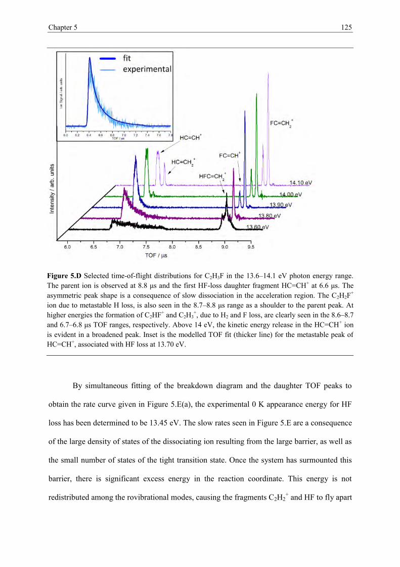
Chapter 5 125

Figure 5.D Selected time-of-flight distributions for C2H3F in the 13.6–14.1 eV photon energy range. The parent ion is observed at 8.8 μs and the first HF-loss daughter fragment HC=CH+ at 6.6 μs. The asymmetric peak shape is a consequence of slow dissociation in the acceleration region. The C2H2F+ ion due to metastable H loss, is also seen in the 8.7–8.8 μs range as a shoulder to the parent peak. At higher energies the formation of C2HF+ and C2H3

+, due to H2 and F loss, are clearly seen in the 8.6–8.7 and 6.7–6.8 μs TOF ranges, respectively. Above 14 eV, the kinetic energy release in the HC=CH+ ion is evident in a broadened peak. Inset is the modelled TOF fit (thicker line) for the metastable peak of HC=CH+, associated with HF loss at 13.70 eV.

By simultaneous fitting of the breakdown diagram and the daughter TOF peaks to

obtain the rate curve given in Figure 5.E(a), the experimental 0 K appearance energy for HF

loss has been determined to be 13.45 eV. The slow rates seen in Figure 5.E are a consequence

of the large density of states of the dissociating ion resulting from the large barrier, as well as

the small number of states of the tight transition state. Once the system has surmounted this

barrier, there is significant excess energy in the reaction coordinate. This energy is not

redistributed among the rovibrational modes, causing the fragments C2H2+ and HF to fly apart

Chapter 5 126

with considerable translational kinetic energy. The experimental 0 K appearance energy and

the calculated endothermicity of the dissociative photoionization yield a reverse barrier to HF

loss of 1.14 eV. This can be compared with a purely ab initio derived barrier of 1.34 eV,

Figure 5.B(a).

Figure 5.E. Plot of log10 k(E) vs. hv for (a) HF loss and H loss from C2H3F+, (b) HF loss and F loss from 1,1-C2H2F2

+. The experimental rates, observed in the 103 s−1 < k < 107 s−1 range, are extrapolated to obtain the E0.

The G3B3 calculated onset for H-atom loss, CHF=CH2 → C2H2F+ + H + e–, is 13.67

eV when the hydrogen atom is lost from the fluorinated carbon [1] → [5], and 14.71 eV when

it is lost from the CH2 group. The 0 K appearance energy of this daughter ion (m/z 45) is

experimentally determined to be 13.60 eV, suggesting that the former hydrogen atom loss

process giving rise to C2H2F+ is not kinetically hindered. Indeed, no reverse barrier to

hydrogen atom loss could be found in our calculations, thus the metastable decay close to

threshold, see rate data in Figure 5.E(a), is mostly due to the large barrier and the

correspondingly large density of states in the parent ion. The observation of this metastability

supports results reported by Güthe et al.9 Since the H-loss transition state is looser than the

HF-loss one, the competition between the first two channels favours the former, with the

Chapter 5 127

C2H2F+ fractional abundance some 20% higher than that C2H2+ between 14–18 eV. Above

18.4 eV the loss of 20 a.m.u. becomes the dominant channel. This is identified as the

formation of HC=CH+ + H + F + e–, for which the G3B3 calculated onset is 18.19 eV. The

reaction endothermicity of CHF=CH2 → H2C=C+ + H + F + e– is calculated to be 19.99 eV,

and is subsequently discounted as the origin of the signal below 20 eV. Consequently the m/z

26 daughter ion C2H2+ is derived from the sequential dissociation of C2H3

+ by H loss as well

as from C2H2F+ by F loss in this energy range.

From their threshold to about 0.5 eV above, the fractional ion abundances of C2HF+

and C2H3+ rise less steeply than those of the first two daughter ions, C2H2

+ and C2H2F+. The

appearance energy, AE, of C2HF+ and C2H3+ are measured to be 13.7 and 13.9 eV,

respectively. The thermochemical onset for 2,2-H2 elimination yielding FHC=C+ is calculated

to be 15.62 eV and cannot take place in this energy range. Therefore the structure of C2HF+

must be CF=CH+, which is confirmed by the calculated 1,2-H2 elimination threshold of 13.68

eV. Contrary to 1,1-difluoroethene, in which only 2,2-H2 elimination is structurally possible,

H2 loss can compete effectively with the other dissociation channels in monofluoroethene.

The agreement between the calculated and the experimental onsets also suggest that H2 loss is

not slow at threshold, quite unlike HF loss. This is only possible if H2 loss has no reverse

barrier along the reaction coordinate, or if it is very narrow and there is fast tunnelling

through it.

The mechanism of F loss yielding C2H3+ has been discussed extensively in the

literature.8,9,34,35 This process is observed at its thermochemical threshold, and its rise is

consistent with a statistical competitive fast reaction with a loose transition state. As can be

seen in the TOF distributions (Figure 5.E), the parent ion ceases to be metastable in this

energy range and the F-loss signal is readily identified in our experiment, in contrast to a

previous report.9 However, at 15.5 eV, there is a sudden increase in the C2H3+ abundance

Chapter 5 128

which fits poorly into the statistical picture. Previously, it was proposed that isolated state

behaviour (i.e. the dissociation dynamics are dominated by those of the electronic state of

the parent ion) contributes to this signal.8,34,35 However, the peak in the TPES is observed

at an onset of 16.18 eV, whereas this sudden rise occurs some 0.7 eV lower, still in the

energy range of the peak. Furthermore, the C2H3+ ion abundance follows the peak only

very approximately. Consequently, we confirm the double nature of the F-loss process, but

also suggest that the state is not playing a simple and direct role in the non-statistical range.

Instead of state participation, it is more likely that Rydberg series converging to the state

have different autoionization pathways leading to the C2H3+ product. Based on the KER

analysis of the C2H3+ ion yield at 16.85 eV, Momigny and Locht35 conclude that

approximately two thirds of the ion flux dissociates on the state producing the

electronically excited state of C2H3+, which can then internally convert to its ground

state, thereby keeping most of the excess energy. However one third of the ion flux arrives at

the ground state of C2H3F+, which correlates with the ground state of C2H3+, allowing

for a larger kinetic energy release. Such a bimodal behaviour has also been proposed by

Gridelet et al. for the F-loss pathway from 1,1-C2H2F2+.14 Indeed, there is a very swift

decrease in half the C2H3+ signal together with a jump in the C2H2

+ fractional abundance at

around hν = 18.5 eV. Taking into account the 0 K heats of formation of C2H3+,36 C2H2

+,31,32

and H,37 (1120, 1329 and 216 kJ mol–1, respectively), C2H3+ is expected to lose a further H

atom at an internal energy of 4.4 eV, i.e. at a photon energy of 18.4 eV, whilst the G3B3

value for the dissociative photoionization C2H3F HC=CH+ + F + H + e– is 18.19 eV. As

will be shown later for C2F4, the breakdown diagram of a sequential dissociation corresponds

to the internal energy distribution in the first dissociation step, and can be used to study the

excess energy redistribution. Thus, we attempted to analyse the C2H3+ vs. C2H2

+ breakdown

curves in the 18–19 eV range to determine the C2H3+ internal energy distribution. There is a

Chapter 5 129

difference of about 1 eV in the excess energy available for kinetic energy release depending

on whether the excited or ground state C2H3+ intermediate is formed. Both pathways yielded

an acceptable fit to the C2H2+ breakdown curve within the signal-to-noise ratio of the

experimental data. Ergo, the comparatively noisy high-energy breakdown curves of the three

different open channels (H + F loss, F + H loss with an or C2H3+ intermediate)

and the small differences in their energies (1.3 and 1 eV more excess energy available for

KER in the first two) do not allow for a sufficiently detailed description of the reaction

mechanism yielding C2H2+.

CF+ (m/z 31) appears around a photon energy of 14.87 eV, which is 0.3 eV higher

than the G3B3 calculated endothermicity for CHF=CH2 → CF+ + CH3 + e–, 14.56 eV. It is

0.17 eV higher than the previously reported thermochemical value of 14.704 eV9 and lies

between previous appearance energies of 14.5 eV8 and 14.90 eV.9 Methyl radical loss is

preceded by H atom migration, and ab initio calculations were used to obtain a plausible

pathway to CF+ production. The transition state to CF−CH3+ was calculated to lie at 12.07

eV, well below the overall barrier to CF+ formation. The highest energy major channel

observed in this work is C=C bond cleavage to form CHF+ + CH2. It has a calculated onset

energy of 17.38 eV and is seen experimentally at 18.4 eV. This value is ca. 2 eV lower than

the appearance energy of 20.02 eV reported by Güthe.9 The thermochemical threshold to

CHF+ + CH2, 17.099 eV,38 is in reasonable agreement with our calculated G3B3 value,

confirming the competitive shift in the CHF+ signal. At such high internal energies numerous

processes can take place at rates comparable to intramolecular vibrational relaxation.

Therefore, the fact that we observe a further parallel channel opening up at all is remarkable.

Chapter 5 130

5.B.2. 1,1-Difluoroethene

Figure 5.F. (a) Breakdown diagram and TPES of 1,1-C2H2F2 over the range 13.9 to 21.0 eV. The G3B3 calculated onsets at 0 K for selected fragment ions are also included. (b) Modelled fit (solid line) with experimental points (open shapes) for the parent ion, 1,1-C2H2F2

+, and the onsets for the first two daughter ions, FC=CH+ and C2H2F+ in the 13.9–14.7 eV energy range.

The breakdown diagram of 1,1-C2H2F2+ in the 13.9−21.0 eV energy range with ab

initio dissociative photoionization energies for selected channels, as well as the experimental

Chapter 5 131

and modelled breakdown curves for the HF and F loss reactions in the 13.9–14.7 eV energy

range, are shown in Figure 5.F. Similarly to monofluoroethene, HF loss is the lowest energy

channel and the G3B3 calculated endothermicity lies 1.4 eV lower than that for F-atom loss.

The calculated reaction energy for F2C=CH2 → FC=CH+ + HF + e– at 0 K is 13.04 eV and

the experimental 0 K onset energy, obtained by simultaneous modelling of the breakdown

diagram and the daughter ion TOF spectra, is 14.05 eV. This agrees with the value of 14.1 eV

reported by Güthe,9 and indicates a reverse barrier of 1.01 eV in [2] → [14]‡ → [15]. The

daughter ion TOF peak shapes indicate metastable behaviour, and our calculations predict a

tight transition state. The purely calculated Erb of 1.19 eV is, as for C2H3F+, somewhat higher

than the value based on the experimental E0. This small discrepancy of 0.18 eV could be

explained by tunnelling through the reverse barrier, which effectively lowers the observed E0.

Our values agree with the previously measured Erb of 0.98 eV but not with the reported ab

initio value of 1.69 eV.10,11 This indicates that most of the reported 0.71 eV difference was

primarily due to the inadequate description of the potential energy surface at the UHF/6-

31G(d)//UHF/STO-3G level of theory.

The calculated onset energy for the formation of C2H2F+ (m/z 45) by F loss is 14.40

eV. The corresponding breakdown curve, however, is noisy due to the background

subtraction required because the large asymmetric TOF signal of FC=CH+ overlaps with the

FC=CH2+ signal from F-loss (Figure 5.G). We performed a potential energy scan along the

C–F bond stretch coordinate to obtain the potential energy curve for F-atom loss. Figure

5.B(b) shows that a transition state at a C–F bond length of 1.8 Å is predicted [11]‡, in which

the leaving fluorine atom straddles the C=C bond. This transition state may lead either to F-

loss (in which there is no overall reverse barrier) or to the CH2F–CF+ isomer ion [9].

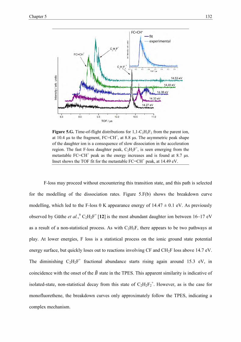
Chapter 5 132

Figure 5.G. Time-of-flight distributions for 1,1-C2H2F2 from the parent ion, at 10.4 μs to the fragment, FC=CH+, at 8.8 μs. The asymmetric peak shape of the daughter ion is a consequence of slow dissociation in the acceleration region. The fast F-loss daughter peak, C2H2F+, is seen emerging from the metastable FC=CH+ peak as the energy increases and is found at 8.7 μs. Inset shows the TOF fit for the metastable FC=CH+ peak, at 14.49 eV.

F-loss may proceed without encountering this transition state, and this path is selected

for the modelling of the dissociation rates. Figure 5.F(b) shows the breakdown curve

modelling, which led to the F-loss 0 K appearance energy of 14.47 ± 0.1 eV. As previously

observed by Güthe et al.,9 C2H2F+ [12] is the most abundant daughter ion between 16–17 eV

as a result of a non-statistical process. As with C2H3F, there appears to be two pathways at

play. At lower energies, F loss is a statistical process on the ionic ground state potential

energy surface, but quickly loses out to reactions involving CF and CH2F loss above 14.7 eV.

The diminishing C2H2F+ fractional abundance starts rising again around 15.3 eV, in

coincidence with the onset of the state in the TPES. This apparent similarity is indicative of

isolated-state, non-statistical decay from this state of C2H2F2+. However, as is the case for

monofluorethene, the breakdown curves only approximately follow the TPES, indicating a

complex mechanism.

Chapter 5 133

The G3B3 onset energies for CH2F+ and CF+ are close to one another at 14.82 eV and

14.92 eV, and their experimental onsets are 14.70 and 14.86 eV, respectively. These daughter

ions are the products of the same process with the charge localised on one or the other

fragment. The CF+ and CH2F+ fragments are formed in competition with fast F and HF loss,

suggesting a loose transition state and no overall reverse barrier to dissociation. As already

mentioned, in the transition state structure the F atom can move over and attach to the CH2

group in [11]‡, [2] → [11]‡ → [9] → [10]. C–C bond rupture in [11]‡ can also lead to CF+.

The ionization energy (IE) of CF has been determined by Dyke et al to be 9.11 ± 0.01 eV,39

whereas that of CH2F is reported to be 9.04 ± 0.01 eV by Andrews et al.40 In the absence of a

competitive shift, the offset in onset values would correspond to the ionization energy

difference. If there is a competitive shift, i.e. the CF+ signal is delayed and rises only at

higher energies because it is outcompeted by the other parallel channels, this offset can only

be considered as an upper limit to the ionization energy difference. Both quantities appear to

be well established; hence in lieu of a detailed kinetic model, only a lower limit to the IE of

CH2F is given as 8.95 eV. At energies above 15.3 eV, the signal for these two ions decreases

because the non-statistical F-loss channel is preferred.

The calculated onsets of the H-loss products (m/z 63), HFC=CF+ and F2C=CH+, are

15.24 eV and 15.52 eV, respectively. Experimentally, H-loss product appears only at a higher

photon energy of ca.15.9 eV, primarily because it is outcompeted by the other fast processes

at lower energies. This also leads to its slow rise with increasing hν. At an energy ~1 eV

lower than in monofluoroethene, cleavage of the C=C bond occurs. The calculated onset for

production of CH2+ + CF2 is 15.96 eV, and its experimental appearance energy is 16.9 eV. By

contrast, the CH2 loss is calculated at 17.42 eV but is not seen experimentally until 18.9 eV.

The faster rise of CH2+ than that of C2HF2

+ from H loss suggests a looser transition state for

the C=C bond rupture. Unlike monofluoroethene, however, the positively charged fragment

Chapter 5 134

first seen resulting from C=C cleavage is not the fluorine-containing moiety, but CH2+. This

observation is explained by the 1.3 eV difference between the IE of these fragments (CH241

10.39 ± 0.01 eV, CHF42 10.06 ± 0.05 eV, CF243 11.36 ± 0.005 eV).

Based on energetics considerations, the second rise in the CF+ signal at 19 eV is

suggested to stem mostly from the C−C bond cleavage in the H-loss fragment ion, HFC=CF+

(calculated onset is 18.96 eV). This is supported by a decrease in the C2HF2+ abundance in

this energy range, i.e. a decrease in the H-loss signal. Finally, the decrease in the F-loss signal

C2H2F+ between 19 and 20 eV is due to two possible consecutive reactions from C2H2F+: a

further H-loss to FC=CH+ (18.91 eV), or, after a rearrangement to HFC=CH+, a loss of F to

HC=CH+ (18.92 eV) in agreement with the mechanism suggested by Güthe et al.9

5.B.3. Trifluoroethene

To the best of our knowledge, this is the first report of the fragmentation pathways of

ionized trifluoroethene by coincidence techniques. The breakdown diagram and the threshold

photoelectron spectrum in the 13.5–21.5 eV photon energy range are shown in Figure 5.H(a).

The adiabatic ionization energy of the neutral molecule has been determined to be 10.14

eV.21 The lowest-energy G3B3 calculated 0 K dissociative photoionization energy of 13.47

eV corresponds to the 1,2-HF elimination. In contrast to monofluoroethene and 1,1-

difluoroethene, this reaction is not observed and C2F2+ is virtually absent in the breakdown

diagram.

The first observed daughter ion, CHF2+ corresponds to the loss of the CF fragment

which requires an initial F-atom migration [3] → [16]‡ → [18]. The G3B3 calculated onset

energy is 13.86 and eV the experimental 0 K appearance energy is measured to be 13.856 ±

Chapter 5 135

0.007 eV, so there appears to be no reverse barrier in the exit channel. Figure 5.H(b) shows

the experimental data, the modelled breakdown diagram, and the obtained 0 K appearance

energies determined for the first three dissociation channels. The TOF peaks corresponding to

CHF2+ are almost symmetric, so we conclude that the parent ion is barely metastable along

this reaction coordinate and dissociation is therefore fast. When a rearrangement precedes the

loss of HF in ionized mono- and 1,1-difluoroethene, these reactions have slow rate constants.

Therefore it might seem counterintuitive that the rates for CF loss from ionized

trifluoroethene are not slow. To shed light on this issue, we obtained ab initio potential

energy curves leading to these fragments, see Figure 5.B(c). The F-transfer transition state in

this series has a 3-membered ring structure [11]‡, [16]‡ and [24]‡ whereas HF-loss proceeds

via a 4-membered ring transition state structure [7]‡ and [14]‡. The figure also shows that the

reaction coordinate changes character as the reaction proceeds. Initially, it starts as a F-atom

migration across the C=C bond leading to a HF2C–CF+ minimum, but this is followed by a

C–C bond cleavage to form CHF2+ + CF, [3] → [16]‡ → [17] → [18]. The F-transfer

transition state [16]‡ lies at 12.74 eV and the H-transfer transition state has been found to lie

at 12.93 eV, so both pathways are possible, though the lower energy F-transfer is more

favourable. The reverse barrier associated with the F-migration is much smaller than the

dissociation endothermicity, so there is no overall reverse barrier to production of CHF2+ +

CF or CF+ + CHF2. Thus, the 0 K appearance energy of CHF2+, 13.856 ± 0.007 eV,

corresponds to the dissociative photoionization energy.

Chapter 5 136

Figure 5.H (a) Breakdown diagram and TPES of C2HF3 over the range 13.45 to 21.5 eV. The G3B3 calculated onsets at 0 K for selected fragment ions are also included. The calculated onset for the 1,2-HF abstraction at 13.47 eV denoted by the black dashed line, is included for reference, though the product ion is not seen experimentally. (b) Experimental points (open shapes) with modelled breakdown curve (solid line) for C2HF3

+, and the onsets for the first three daughter ions, CHF2

+, CF+ and CHF+ in the energy range 13.50–15.25 eV.

The second daughter ion observed is CF+, corresponding to the loss of the CHF2

fragment, [3] → [16]‡ → [17] → [19]. The experimentally determined 0 K appearance energy

for this ion is 14.16 ± 0.02 eV, with the G3B3 onset energy calculated to be 14.33 eV. As

Chapter 5 137

these first two dissociative photoionization reactions differ only in which moiety the positive

charge is localized on, the difference in the E0 values, 0.30 ± 0.02 eV, yields the difference in

the ionization energies of the CF and CHF2 radicals. The ionization energy of CF is well

established, 9.11 eV ± 0.01,39 whilst values for CHF2 span a large range of experimental

values, 8.78,38 8.74,44 and 10.5 eV,45 and a calculated value of 8.4 eV.46 By anchoring to the

CF value, we determine the IE of the CHF2 radical to be 8.81 ± 0.02 eV. The abundance of

CF+ has two maxima, the first at ca. 15.3 eV (fractional abundance of 25%) and a much

larger one at ca. 20.5 eV (80%). The shape of its breakdown curve can help understand its

production mechanism. At low energies, CF+ is produced by the HFC=CF2 + hν → CF+ +

CHF2 + e– reaction. At 17 eV, a new channel opens up in which the third daughter ion, CHF+,

which is produced initially by C=C bond cleavage to form CHF+ + CF2, loses an H atom in a

sequential process to produce CF+. At 19.1 eV, the steepness of the CF+ yield further

increases as C=C bond rupture becomes possible from the F-loss daughter ion CHF=CF+.

The 0 K appearance energy of the third daughter ion, CHF+ is 14.54 ± 0.02 eV. G3B3

calculations give 14.94 eV, corresponding to cleavage of the C=C bond of the parent ion,

with CF2 as the neutral fragment, [3] → [21]. This process occurs at relatively low photon

energies for trifluoroethene and is an example of the perfluoro-effect,47 i.e. a decrease in the

C=C bond strength as the number of F substituents increases. The onset for CH2+ production

from 1,1-difluoroethene is at ca. 17 eV, the onset of CHF+ from monofluoroethene does not

occur until 18 eV. For all three molecules, however, this never becomes a dominant channel,

with the maximum fractional abundance (CH2+ from 1,1-difluoroethene) never exceeding

35%.

The final major fragment ion formed from trifluoroethene is F-loss to HFC=CF+, [3]

→ [20]. Its appearance energy is 15.36 eV and it turns on at its calculated thermochemical

threshold. This reaction channel is associated with non-statistical F-loss, because the F-loss

Chapter 5 138

curve increases too sharply over a narrow energy range to be statistical. This channel is the

most abundant yield between 15.6 and 19.0 eV, and the signal emulates closely that of the

TPES. This range of energies coincides with the / / excited states of the ion where

ionization occurs from C–F orbitals.21 Unlike the F-loss channel observed from C2H3F+ and

1,1-C2H2F2+, the contribution of the statistical F loss is not seen and is suggested to be minor

at all energies. Higher-energy channels with abundances less than 25% occur after these four

major channels: these are the production of CF2+ + CHF at 17.2 eV and C2HF+ + 2 F at 18.9

eV. G3B3 dissociative photoionization energies for these channels have been calculated to be

16.09 and 19.00 eV, respectively.

5.B.4. Tetrafluoroethene

The first three dissociative photoionization channels of C2F4 open in a Franck–

Condon gap, as shown in the breakdown diagram and threshold photoelectron spectrum,

Figure 5.I(a). This observation is in agreement with the findings of an earlier TPEPICO study

by Jarvis et al.5 The first channel, formation of CF3+ with CF as the accompanying neutral,

has a calculated onset energy of 13.75 eV. Surprisingly, although analogously to the C2HF3

system, the CF3+ TOF peak is symmetric and narrow, therefore the fluorine migration and

subsequent C–C bond cleavage is a fast process without a large reverse barrier. At somewhat

higher energies, CF+ is the second daughter ion, again mirroring the second dissociative

photoionization channel in trifluoroethene. The adiabatic ionization energy of C2F4 is 10.11 ±

0.01 eV,22 meaning that the total depth of the potential energy well to CF3+ + CF is about

3.64 eV, leading to a high density of states in the dissociating ion. In contrast with

trifluoroethene, no reasonably chosen transition state is loose enough to lead to rates larger

than 107 s–1 at such high internal energies.

Chapter 5 139

This indicates that the F-transfer mechanism plays a crucial role in ensuring that there

is no kinetic shift. Rearrangement to a CF3CF+ intermediate, [4] → [24]‡ → [23], can take

place at a much lower energy than the E0 of CF3+. Even though the transition state for this

process is relatively tight, the rates are fast at an excess energy of 1–2 eV, i.e. at the

dissociative photoionization onset: ab initio RRKM rates, based on the G3B3 calculated

transition state are in excess of 109 s−1 at threshold. C–C bond rupture can then proceed

through a loose transition state with a lower density of states in the dissociating intermediate,

giving rise to fast rates and no kinetic shift for [4] → [24]‡ → [23] → [22] or [25]. In the

absence of this CF3CF+ intermediate [23], the dissociation would be slow and a kinetic shift

apparent in the spectrum. Figure 5.I(b) shows the modelled breakdown curves, and the E0 for

CF3+ production has been determined to be 13.717 ± 0.007 eV.

The appearance energy of CF3+ and that of the second daughter, CF+, are very close,

as the ionization energy of CF3, somewhat controversially reported as 8.61 eV,48 8.6−8.7

eV,49 9.04 eV,50 9.05 ± 0.004 eV,51 9.02 ± 0.03 eV and 9.08 ± 0.03 eV,52 is only slightly

lower than that of CF, 9.11 ± 0.01 eV.39 The E0 to CF+ + CF3 formation is determined to be

13.740 ± 0.010 eV based on the statistical modelling. The difference between the barriers to

these two daughter ions is 0.023 eV, and, together with the IE of CF, the IE of CF3 is

determined to be 9.090 ± 0.015 eV. This lies towards the higher end of previous reported

onset values. While our CF3+ E0 agrees well with the result from the photoionization

efficiency (PIE) curve of C2F4 of 13.721 ± 0.005 eV,51 our CF+ onset differs considerably

from the value of 13.777 ± 0.005 eV reported by Asher and Ruscic.51 Presumably, the reason

is that the competitive shift in the CF+ channel was not considered in the PIE work, leading to

a higher reported value. As a consequence, an onset energy difference (0.055 ± 0.003 eV)

was reported, which corresponds well to the offset in breakdown curves we observe, but not

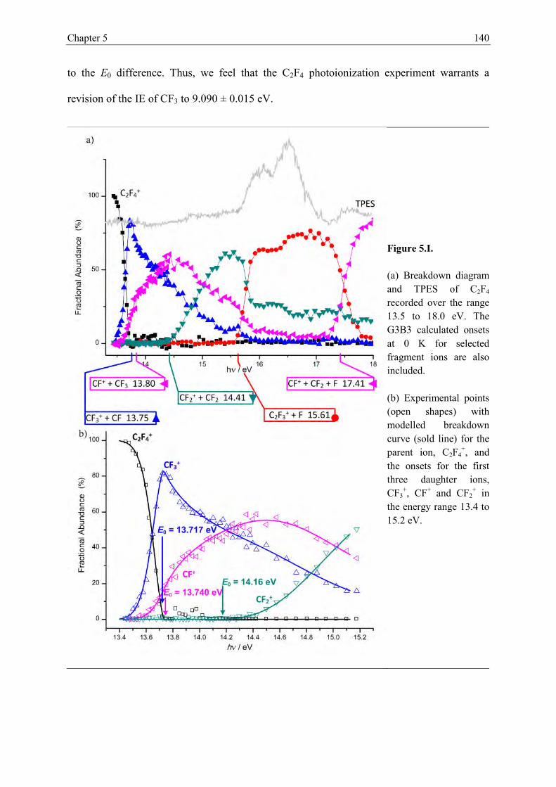
Chapter 5 140

to the E0 difference. Thus, we feel that the C2F4 photoionization experiment warrants a

revision of the IE of CF3 to 9.090 ± 0.015 eV.

Figure 5.I. (a) Breakdown diagram and TPES of C2F4 recorded over the range 13.5 to 18.0 eV. The G3B3 calculated onsets at 0 K for selected fragment ions are also included. (b) Experimental points (open shapes) with modelled breakdown curve (sold line) for the parent ion, C2F4

+, and the onsets for the first three daughter ions, CF3

+, CF+ and CF2+ in

the energy range 13.4 to 15.2 eV.

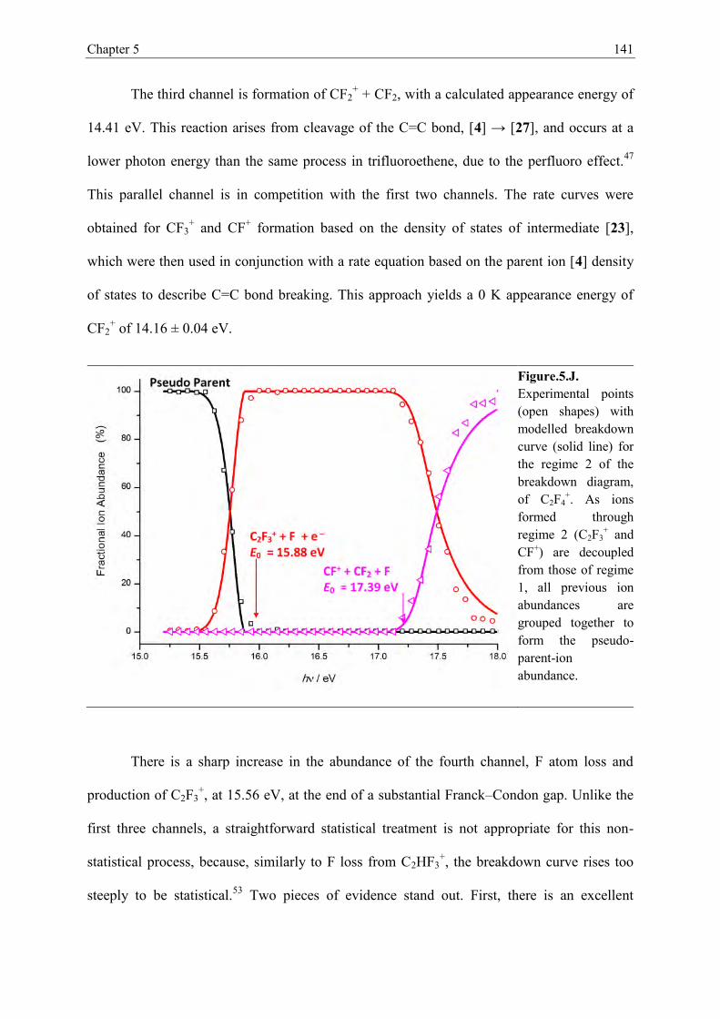
Chapter 5 141

The third channel is formation of CF2+ + CF2, with a calculated appearance energy of

14.41 eV. This reaction arises from cleavage of the C=C bond, [4] → [27], and occurs at a

lower photon energy than the same process in trifluoroethene, due to the perfluoro effect.47

This parallel channel is in competition with the first two channels. The rate curves were

obtained for CF3+ and CF+ formation based on the density of states of intermediate [23],

which were then used in conjunction with a rate equation based on the parent ion [4] density

of states to describe C=C bond breaking. This approach yields a 0 K appearance energy of

CF2+ of 14.16 ± 0.04 eV.

Figure.5.J. Experimental points (open shapes) with modelled breakdown curve (solid line) for the regime 2 of the breakdown diagram, of C2F4

+. As ions formed through regime 2 (C2F3

+ and CF+) are decoupled from those of regime 1, all previous ion abundances are grouped together to form the pseudo-parent-ion abundance.

There is a sharp increase in the abundance of the fourth channel, F atom loss and

production of C2F3+, at 15.56 eV, at the end of a substantial Franck–Condon gap. Unlike the

first three channels, a straightforward statistical treatment is not appropriate for this non-

statistical process, because, similarly to F loss from C2HF3+, the breakdown curve rises too

steeply to be statistical.53 Two pieces of evidence stand out. First, there is an excellent

Chapter 5 142

correlation between the peaks in the TPES and the breakdown curve here. Second, the

steepness of the crossover region is not only inconsistent with a parallel competing channel,

but, as will be shown later, also corresponds to the room temperature internal energy

distribution of C2F4+; significantly unlike a crossover due to a slowly changing rate constant

ratio of competing statistical processes. The overall breakdown diagram appears to be

comprised of two separate outcomes or regimes. The first one consists of the CF3+ + CF, CF+

+ CF3 and CF2+ + CF2 channels discussed so far, which arise from dissociations on the

ground state surface of the parent ion, C2F4+, partly through the intermediate structure

CF3CF+. Below a photon energy of 15.5 eV, only reactions belonging to this first regime are

observed. Above this energy, a regime change occurs, and the two of the observed reactions

belong to the excited, isolated-state second regime: loss of a fluorine atom yielding CFCF2+ +

F, which is followed by the sequential formation of CF+ + CF2 + F above 17.2 eV.

As seen in the breakdown diagram in the range 15.9–18.0 eV, regime-two reactions

dominate the regime-one reactions by a constant factor of roughly 2:1. The threshold

photoionization mechanism is suggested to play a vital role and can be discussed in the

framework proposed for iodomethane previously.54 Following photoabsorption, the neutral

C2F4 molecule is excited to a Rydberg state with favourable Franck–Condon factors. Three

non-radiative decay pathways are possible: (1) crossing to a repulsive neutral curve leading to

neutral fragments, which are not detected in our experiment, (2) whilst on this repulsive

surface, the system can return to the ground state Rydberg manifold eventually leading to the

ground state parent ion which dissociates via regime one, and (3) direct autoionization to an

excited electronic state, in this case the state of C2F4+, which dissociates according to

regime two by F loss and then by consecutive CF2 loss.

Here we discuss three aspects of the double-regime dissociation mechanism of C2F4+.

First, in Figure 5.B(d), TD-DFT potential energy levels are shown for production of CF3+ +

Chapter 5 143

CF, the simple C=C bond breaking and the F-loss channels. Excited state potential energy

curves were obtained along the minimum energy path for the ground electronic state, and the

TD-DFT minima and maxima are reported here. These points are therefore not necessarily

stationary points on the excited state surface, but we believe they are reasonably good

representations of them. Some EOM-UCCSD/aug-cc-pVTZ calculations along these curves

showed the same general characteristics with only small differences in excitation energy.

Since the C–F bond is very strong, F loss cannot compete effectively on the ground electronic

surface; the dynamics are dominated by the CF3+ + CF, CF+ + CF3 and CF2

+ + CF2 exit

channels. However, if the first excited state is only weakly coupled to the ground state, which

is hardly surprising given the 4−6 eV gap between the two states, F loss, [26]*→[28],

becomes possible. This is not because the state converges to energetically disallowed

excited state products, as was invoked in the non-statistical model for Sn(CH3)3X25 and

methanol,27 but because of large reverse barriers for the other competing processes on the

excited state surface. Thus, the three regime-one exit channels, [26]* → [31]‡ ↛ [22], [26]*

→ [31]‡ ↛ [25] and [26]* →[29]‡

↛ [27], are kinetically ‘blocked’ on the state surface, see

Figure 5.K.

Second, the narrow width of the regime crossover at 15.9 eV corresponds to the width

of the thermal energy distribution of C2F4+. This observation prompted us to consider the

regime-two processes independently of the preceding channels, and plot a ‘regime-two

breakdown diagram’ as shown in Figure 5.J. This was achieved by disregarding regime-one

product ions at hν > 16 eV, then re-normalizing the signal so that the F-loss daughter ion,

C2F3+, converges to 100% closely above 16 eV.

This is done to obtain a regime-two ‘pseudo parent ion’ signal. The temperature of the

internal energy distribution in the ‘pseudo parent’ that gives the best fit is 340 K, somewhat

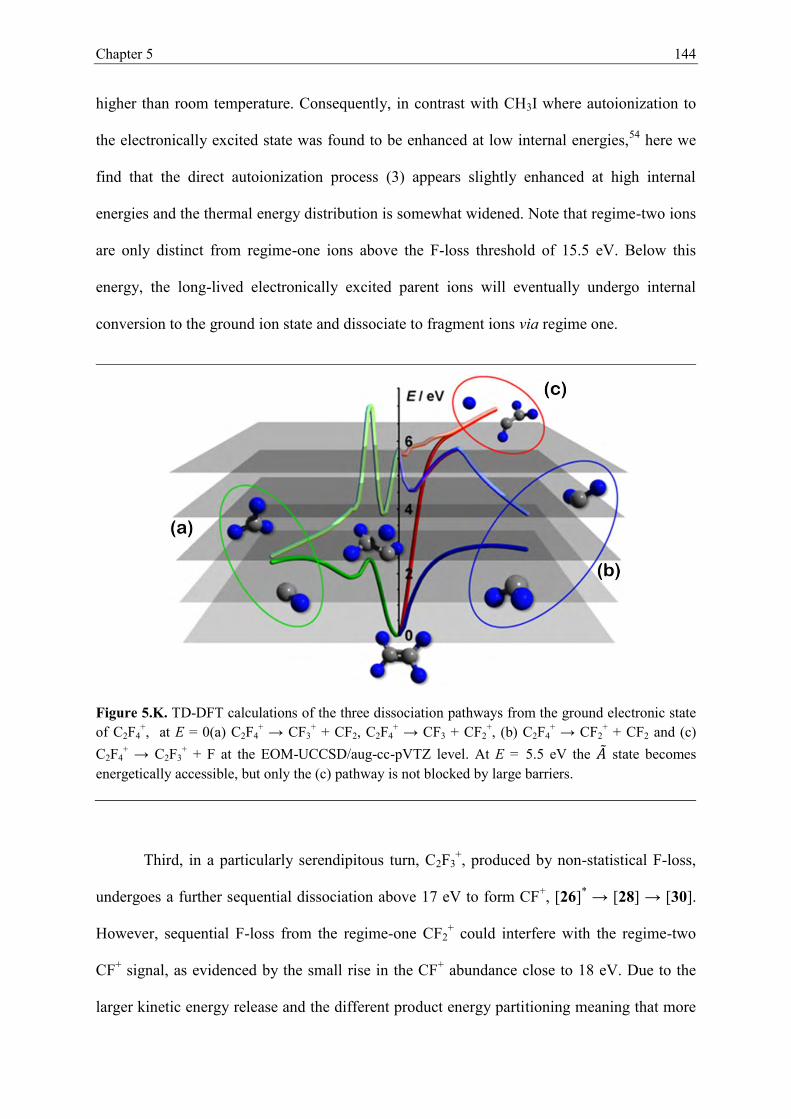
Chapter 5 144

higher than room temperature. Consequently, in contrast with CH3I where autoionization to

the electronically excited state was found to be enhanced at low internal energies,54 here we

find that the direct autoionization process (3) appears slightly enhanced at high internal

energies and the thermal energy distribution is somewhat widened. Note that regime-two ions

are only distinct from regime-one ions above the F-loss threshold of 15.5 eV. Below this

energy, the long-lived electronically excited parent ions will eventually undergo internal

conversion to the ground ion state and dissociate to fragment ions via regime one.

Figure 5.K. TD-DFT calculations of the three dissociation pathways from the ground electronic state of C2F4

+, at E = 0(a) C2F4+ → CF3

+ + CF2, C2F4+ → CF3 + CF2

+, (b) C2F4+ → CF2

+ + CF2 and (c) C2F4

+ → C2F3+ + F at the EOM-UCCSD/aug-cc-pVTZ level. At E = 5.5 eV the state becomes

energetically accessible, but only the (c) pathway is not blocked by large barriers.

Third, in a particularly serendipitous turn, C2F3+, produced by non-statistical F-loss,

undergoes a further sequential dissociation above 17 eV to form CF+, [26]* → [28] → [30].

However, sequential F-loss from the regime-one CF2+ could interfere with the regime-two

CF+ signal, as evidenced by the small rise in the CF+ abundance close to 18 eV. Due to the

larger kinetic energy release and the different product energy partitioning meaning that more

Chapter 5 145

than half of the excess energy is lost in the first C=C bond rupture step, this regime-one

process will be very slow to rise with increasing photon energy, confirmed by the almost

constant CF2+ abundance above 17.5 eV. Therefore, regime-two processes are virtually

distinct from regime-one processes.

Repulsive surfaces and impulsive mechanisms are often invoked to explain effective

competition between non-statistical and statistical channels.55 It was only recently that some

evidence has been published highlighting the statistical redistribution of internal energy

which is possible in isolated-state processes.27 The breakdown curve of a sequential

dissociation yields the product energy distribution of the dissociating ion.17,25 By modelling

the second step in the regime-two breakdown diagram in Figure 5.J, it becomes evident that it

is only the electronic ground state phase space which is inaccessible to our system, and

statistical redistribution of the excess energy among the nuclear degrees of freedom can

indeed occur. The derived E0 values of 15.88 ± 0.03 eV and 17.39 ± 0.06 eV for C2F3+ + F

and CF+ + CF2 + F, respectively, can be compared with the G3B3 calculated dissociative

photoionization energies of 15.61 and 17.41 eV. The enthalpies of formation for C2F4, CF+,

CF2 and F as listed in Table 5.1 yield an onset for C2F4 → CF+ + CF2 + F of 17.32 ± 0.06 eV

supporting the E0 derived in this work. This agreement is excellent, confirming the validity of

the ‘pseudo-parent assumption’ and the applicability of the statistical approach to regime two.

To summarize, the internal energy distribution of the F-loss daughter ion, C2F3+, determines

its breakdown curve in the sequential CF2-loss process. The latter is very well described

assuming a statistical redistribution of the excess energy in the F-loss step. Therefore the F-

loss is found to be non-statistical only in the sense that the ground electronic state is

inaccessible. The statistical approximation is valid for the nuclear degrees of freedom, and F

loss is not an impulsive process as was previously proposed.5

Chapter 5 146

5.B.5. Trends and insights into bonding

We consider five statistical dissociation channels on the ground electronic state and non-

statistical F-loss from excited electronic states in C2H4–nFn+. The former channels comprise:

(1) C–H bond cleavage, (2) statistical C–F bond cleavage, (3) HF loss by way of a four-

membered ring transition state, (4) C–C bond cleavage by way of a three-membered ring

transition state, and (5) C=C bond cleavage.

The C–H bond becomes progressively stronger with increasing n. In trifluoroethene,

with a G3B3 calculated H-loss onset of 15.48 eV, the C−H bond is already too strong to

compete successfully with the other dissociation channels. The F-loss potential energy well

also deepens in the group with increasing n. In mono- and difluoroethene, statistical F-loss

competes effectively, whereas statistical F-loss is at most a minor channel in trifluoroethene,

and absent in C2F4+. In fact, non-statistical F-loss establishes a second dissociation regime in

C2F4+, in which only the ground electronic state is inaccessible to the reactive flux.

Four-membered ring CHFC transition states may lead to HF loss in n = 1–3, which is

the least endothermic channel, albeit with a decreasing margin as n increases, and is absent in

the trifluoroethene breakdown diagram because of the large barrier to forming the transition

structure. In short, the four-membered ring transition structure is destabilised as n

increases. Three-membered ring transition states lead to F/H-migration and subsequent C–C

bond breaking. The F-transfer transition state in trifluoroethene is calculated to be 0.19 eV

lower in energy than H-transfer, but H-transfer may still compete if the tunnelling through the

barrier is sufficiently fast. With increasing F-substitution, the three-membered ring

transition states are found to be stabilised, and the resulting fragments dominate the low-

energy breakdown diagram in n = 3 and 4. In contrast with the four-membered ring HF-loss

transition state, F-migration takes place at internal energies below the C–C bond energy. This

Chapter 5 147

means that the corresponding dissociative photoionization processes are fast, and their

endothermicities can be determined based on the breakdown diagram.

Finally, the C=C bond energy decreases from n = 3 to n = 4 as predicted by the

perfluoro effect.47 C=C bond rupture is a minor channel in monofluoroethene, a significant

one in n = 2, hardly observed for n = 3, and becomes one of the major regime-one channels in

tetrafluoroethene.

5.B.6. Thermochemistry

For the dissociative photoionization reaction AB + hν A+ + B + e−, the enthalpy of

the unimolecular reaction, ∆rHo, and the appearance energy of the daughter ion A+, E0, are

equivalent only at 0 K and in the absence of a reverse barrier, see Figure 5.A(a);

(5.2)

Therefore, using 0 K appearance energies with established enthalpies of formation for neutral

parent molecules, neutral fragments and daughter ions, the 0 K enthalpy of formation of the

least well-determined species can be obtained.

To convert the enthalpy of formation of a molecular species or ion [AB] between 0 K

and 298 K we use

(5.3)

where the thermal correction for a non-linear molecule is defined as

Chapter 5 148

(

)

∑

(

)

∑

(

)

(5.4)

The electron value of (H298K – H0K) is neglected in Eq. 3, i.e. we use the stationary electron

(or ion) convention for ions at T > 0 K.38

We cannot deduce any thermochemical values from C2H3F+ because of the slow HF

loss and insufficient resolution of the H-loss signal due to the broadened parent TOF signal.

Values derived from the other three molecules can be found in Table 5.1. In 1,1-

difluoroethene, the E0 value for F loss, 14.47 ± 0.1 eV, and ∆fHo0K (1,1-C2H2F2) = −343.1 ±

2.5 kJ mol−1,56 yield ∆fHo0K (CH2=CF+) = 976 ± 9 kJ mol−1, converted to 973 ± 9 kJ mol−1 at

298 K. This last value can be compared with the previous room temperature value of 951 kJ

mol−1.38

For tetrafluoroethene, ∆fHo0K (C2F4) = −669.4 ± 3.3 kJ mol−1,56 the C2F4

→ CF3+ + CF

+ e− E0 value of 13.717 ± 0.007 eV, and ∆fHo0K (CF3

+) = 413.4 ± 2.0 kJ mol−1,52 yield ∆fHo0K

(CF) =240.7 ± 3.9 kJ mol−1. This is an improved value upon that of Asher and Ruscic,51 of

251.0 ± 4.6 kJ mol−1, partly because they used an outdated JANAF value which was 14 kJ

mol−1 too high and partly because they overestimated the CF+/CF3+ onset energy difference;

thus they underestimated the CF3 ionization energy by 0.04 eV. From the C2F4 → CF+ + CF3

+ e− E0 value of 13.740 ± 0.010 eV, using ∆fHo0K (CF3) = −462.8 ± 2.1 kJ mol−1,57 we present

an improved value of ∆fHo0K (CF+) = 1119.1 ± 4.0 kJ mol−1. This is in close agreement to the

Burcat value of 1121.9 ± 0.9 kJ mol−1 at 0 K,31 though some distance from the Lias and

JANAF values of 1131.0 and 1140.0 ± 0.5 kJ mol−1 respectively.38,58 Using the C2F4 → CF2

+

+ CF2 + e– E0 value of 14.16 ± 0.04 eV, the IE of CF2 of 11.362 ± 0.03 eV43 and ∆fHo0K

(C2F4) of –669.4 ± 3.3 kJ mol–1,56 we obtain ∆fHo0K (CF2) = –199.7 ± 5.6 kJ mol–1. This value

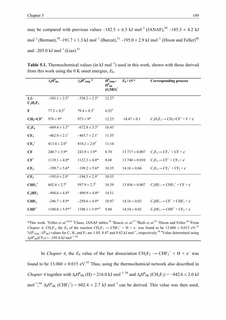
Chapter 5 149

may be compared with previous values –182.5 ± 6.3 kJ mol–1 (JANAF),58 –185.3 ± 4.2 kJ

mol–1 (Berman),59–191.7 ± 1.3 kJ mol–1 (Burcat),31 –195.0 ± 2.9 kJ mol–1 (Dixon and Feller)60

and –205.0 kJ mol–1 (Lias).61

Table 5.1. Thermochemical values (in kJ mol−1) used in this work, shown with those derived from this work using the 0 K onset energies, E0.

∆fHo0K ∆fHo

298K g Ho298K–

Ho0K

(G3B3)*

E0 / eV* Corresponding process

1,1-C2H2F2

–343.1 ± 2.5a –350.2 ± 2.5a 12.27

F 77.3 ± 0.3b 79.4 ± 0.3b 6.52b

CH2=CF+ 976 ± 9* 973 ± 9* 12.25 14.47 ± 0.1 C2H2F2 → CH2=CF+ + F + e–

C2F4 –669.4 ± 3.3a –672.8 ± 3.3a 16.43

CF3 –462.8 ± 2.1c –465.7 ± 2.1c 11.55

CF3+

413.4 ± 2.0d 410.2 ± 2.0d 11.14

CF 240.7 ± 3.9* 243.9 ± 3.9* 8.70 13.717 ± 0.007 C2F4 → CF3

+ + CF + e–

CF+ 1119.1 ± 4.0* 1122.3 ± 4.0* 8.68 13.740 ± 0.010 C2F4 → CF+ + CF3 + e–

CF2 –199.7 ± 5.6* −199.2 ± 5.6* 10.35 14.16 ± 0.04 C2F4 → CF2

+ + CF2 + e–

CF2 –195.0 ± 2.9e –194.5 ± 2.9e 10.35

CHF2+ 602.4 ± 2.7f 597.9 ± 2.7f 10.39 13.856 ± 0.007 C2HF3

→ CHF2+ + CF + e–

C2HF3 –494.6 ± 4.8* −499.9 ± 4.8* 14.31

CHF2 –246.7 ± 4.9* –250.6 ± 4.9* 10.97 14.16 ± 0.03 C2HF3 → CF+ + CHF2 + e–

CHF+ 1108.0 ± 5.9*,h 1108.1 ± 5.9*,h 9.80 14.54 ± 0.02 C2HF3 → CHF+ + CF2 + e–

*This work. aFeller et al.56,62 bChase, JANAF tables.58 cRuscic et al.57 dBodi et al.52 eDixon and Feller.60 fFrom Chapter 4, CH2F2, the E0 of the reaction CH2F2 → CHF2

+ + H + e– was found to be 13.060 ± 0.015 eV.63 g(Hº298K –Hº0K) values for C, H2 and F2 are 1.05, 8.47 and 8.82 kJ mol–1, respectively.58 hValue determined using ∆fHo

0K(CF2) = –195.0 kJ mol–1. 60

In Chapter 4, the E0 value of the fast dissociation CH2F2 → CHF2+ + H + e– was

found to be 13.060 ± 0.015 eV.63 Thus, using the thermochemical network also described in

Chapter 4 together with ∆fHo0K (H) = 216.0 kJ mol−1 58 and ∆fHo

0K (CH2F2) = −442.6 ± 2.0 kJ

mol−1,64 ∆fHo0K (CHF2

+) = 602.4 ± 2.7 kJ mol−1 can be derived. This value was then used,

Chapter 5 150

together with the now obtained ∆fHo0K (CF) = 240.7 ± 3.9 kJ mol−1 and the E0 value for

C2HF3 → CHF2+ + CF + e− of 13.856 ± 0.007 eV in trifluoroethene, to derive ∆fHo

0K (C2HF3)

= −494.6 ± 4.8 kJ mol−1. Burcat31 and Lias38 report −485.5 and −485.7 kJ mol−1 respectively,

for this quantity. From the ∆fHo0K (C2HF3) and ∆fHo

0K (CF+) derived herein, and the C2HF3

→ CF+ + CHF2 + e− 0 K appearance energy of 14.16 ± 0.03 eV, we obtain ∆fHo0K (CHF2) =

−246.7 ± 4.9 kJ mol−1. This value is somewhat less than the values of Lias −233.8 ± 5 kJ

mol−1,38 Burcat – 235.7 kJ mol−1,31 and a more recent ab initio study of −239.4 ± 2.6 kJ

mol−1.64 From the C2HF3 → CHF+ + CF2 + e− threshold of 14.54 ± 0.02 eV, and ∆fHo

0K

(C2HF3) derived in this work, the ∆fHo0K (CHF+) was found to be 1108.0 ± 5.9 kJ mol−1. The

enthalpies of formation derived in this work (asterisked values in Table 5.1) differ from those

given in the journal article where this work has been published, due to the use of the E0 of the

reaction CH2F2 → CHF2+ + H + e– obtained by modelling the breakdown curves from

Chapter 4. The article value used an E0 obtained by eye only.

5.C. Conclusions

The unimolecular dissociation of energy-selected fluorinated ethene cations have been

investigated in the 13–25 eV energy range. Four statistical channels, namely HF loss, F loss,

direct cleavage of the C=C double bond as well as cleavage of the C–C bond post F or H

migration have been discussed in detail, in addition to the non-statistical F-loss channel.

The studied fluorinated ethenes may be divided into two groups, the ‘time bombs’

(monofluoroethene and 1,1-difluoroethene) and the ‘fast dissociators’ (trifluoroethene and

tetrafluoroethene). In the time bombs, the least endothermic HF loss channel is blocked by a

tight 4-membered ring transition state structure. As a result, the parent ions have long

lifetimes in the µs timescale at the onset of dissociative photoionization, succeeded by

Chapter 5 151

impulsive loss of HF with about 1 eV kinetic energy release. The latter is due to the large

reverse barrier, reproduced well by the RAC-RRKM modelled appearance energies. In tri-

and tetrafluoroethene, the two main channels at low energies are the post F/H-transfer C–C

bond cleavages, in which the charge stays on either fragment. These processes are found to

take place without an overall reverse barrier, and by taking into account the competitive shifts

in the breakdown curves and deriving accurate 0 K appearance energies, we obtain the

ionization energy differences for these fragments directly. This is particularly useful in C2F4,

where it leads to a new, self-consistent set of thermochemical values for the

CF/CF3/CF+/CF3+ system, (∆fHo

0K = 240.7 ± 3.9, −462.8 ± 2.1, 1119.1 ± 4.0 and 413.4 ± 2.0

kJ mol−1 respectively). The ionization energy of CHF2 has been re-determined to be 8.81 ±

0.02 eV. The ionization energy of CF3 has also been determined, and at 9.090 ± 0.015 eV is

slightly higher than previous values.

As the C–F bond gets progressively stronger with increasing fluorine substitution,

while the F/H-atom migration transition state becomes stabilized, statistical F loss becomes

less competitive. There is evidence of a higher energy, non-statistical F-loss channel in all

four molecules studied, but it is a dominant and exclusive F-loss channel in C2F4+. Thanks to

a fortunate partitioning of the dissociative photoionization products, we could construct and

model a second, regime-two breakdown diagram, in which a sequential CF2 loss is also

included from the F-loss fragment ion, C2F3+. By measuring the product energy distribution

of the F-loss daughter, we could establish that only the ground electronic state of C2F4+ is

inaccessible in the non-statistical F loss channel. Therefore, the dissociating excited state

C2F4*+ ion is long-lived, and that the excess energy is statistically redistributed among the

nuclear degrees of freedom.

Chapter 5 152

References

(1) Sztáray, B.; Bodi, A.; Baer, T. J. Mass Spectrom. 2010, 45, 1233-1245. (2) Blanksby, S. J.; Ellison, G. B. Acc. Chem. Res 2003, 36, 255 - 263. (3) Takeshita, K. Theor. Chem. Acc. 1999, 101, 343-351. (4) Jarvis, G. K.; Boyle, K. J.; Mayhew, C. A.; Tuckett, R. P. J. Phys. Chem. A. 1998,

102, 3219. (5) Jarvis, G. K.; Boyle, K. J.; Mayhew, C. A.; Tuckett, R. P. J. Phys. Chem. A. 1998,

102, 3230-3237. (6) Jennings, K. R. Org. Mass Spectrom. 1970, 3, 85. (7) Stadelmann, J.-P.; Vogt, J. Int. J. Mass Spectrom. Ion Phys. 1980, 35, 83-89. (8) Dannacher, J.; Schmelzer, A.; Stadelmann, J.-P.; Vogt, J. Int. J. Mass Spectrom. Ion

Phys. 1979, 31, 175-186. (9) Güthe, F.; Locht, R.; Leyh, B.; Baumgärtel, H.; Weitzel, K.-M. J. Phys. Chem. A.

1999, 103, 8404-8412. (10) Güthe, F.; Baumgärtel, H.; Weitzel, K.-M. J. Phys. Chem. A. 2001, 105, 7508-7513. (11) Frenking, G.; Koch, W.; Schaale, M.; Baumgärtel, H. Int. J. Mass Spectrom. Ion

Proc. 1984, 61, 305. (12) Booze, J.; Weitzel, K.-M.; Baer, T. J. Chem. Phys. 1991, 94. (13) Malow, M.; Güthe, F.; Weitzel, K.-M. Phys. Chem. Chem. Phys. 1999, 1, 1425. (14) Gridelet, E.; Dehareng, D.; Locht, R.; Lorquet, A. J.; Lorquet, J. C.; Leyh, B. J. Phys.

Chem. A. 2005, 109, 8225. (15) Bodi, A.; Johnson, M.; Gerber, T.; Gengeliczki, Z.; Sztáray, B.; Baer, T. Rev. Sci.

Instrum. 2009, 80, 034101. (16) Johnson, M.; Bodi, A.; Schulz, L.; Gerber, T. Nucl. Instrum. Methods Phys. Res. A

2009, 610, 597-603. (17) Sztáray, B.; Bodi, A.; Baer, T. J. Mass Spectrom. 2010, 45, 1233 - 1245. (18) Lifshitz, C. Mass Spectrom. Rev. 1982, 1, 309-348. (19) Weitzel, K.-M.; Malow, M.; Jarvis, G. K.; Baer, T.; Song, Y.; Ng, C. Y. J. Chem.

Phys. 1999, 111, 8267-8270. (20) Baer, T.; Sztáray, B.; Kercher, J. P.; Lago, A. F.; Bodi, A.; Skull, C.; Palathinkal, D.

Phys. Chem. Chem. Phys. 2005, 7, 1507-1513. (21) Bieri, G.; Niessen, W. V.; Åsbrink, L.; Svensson, A. Chem. Phys. 1981, 60, 61-79. (22) Buckley, T. J.; Johnson, R. D.; Huie, R. E.; Zhang, Z.; Kuo, S. C.; Klemm, R. B. J.

Phys. Chem. 1995, 99, 4879. (23) Powis, I.; Dutuit, O.; Richard-Viard, M.; Guyon, P. M. J. Chem. Phys. 1990, 92,

1643-1652. (24) Smith, D. M.; Tuckett, R. P.; Yoxall, K. R.; Codling, K.; Hatherly, P. A.; Aarts, J. F.

M.; Stankiewicz, M. J. Chem. Phys. 1994, 101, 10559-10575. (25) Baer, T.; Guerrero, A.; Davalos, J. Z.; Bodi, A. Phys. Chem. Chem. Phys. 2011, 13,

17791. (26) Berkowitz, J. J. Chem. Phys. 1978, 69, 3044-3054. (27) Borkar, S.; Sztáray, B.; Bodi, A. Phys. Chem. Chem. Phys. 2011, 13, 13009-13020. (28) Smith, D. M.; Tuckett, R. P.; Yoxall, K. R.; Codling, K.; Hatherly, P. A. Chem. Phys.

Letts. 1993, 216, 493-502 (29) Shaw, D. A.; Holland, D. M. P. J. Phys. B: At., Mol. Opt. Phys. 2008, 41, 145103 -

145113. (30) Nenner, I.; Guyon, P. M.; Baer, T.; Govers, T. R. J. Chem. Phys. 1980, 72, 439115 -

439121. (31) Burcat, A.; Ruscic, B.September 2005 Third Millennium Ideal Gas and Condensed

Phase Thermochemical Database for Combustion with Updates from Active Thermochemical Tables, ANL-05/20 and TAE 960, Technion-IIT; Aerospace

Chapter 5 153

Engineering, and Argonne National Laboratory, Chemistry Division.September.ftp://ftp.technion.ac.il/pub/supported/aetdd/thermodynamics mirrored at http://garfield.chem.elte.hu/Burcat/burcat.html

(32) Lias, S. G. "Ionization Energy Evaluation". In NIST Chemistry WebBook, NIST Standard Reference Database Number 69; Linstrom, P. J., Mallard, W. G., Eds.; National Institute of Standards and Technology, Gaithersburg MD, 20899; Vol. 2011.

(33) Cox, J. D.; Wagman, D. D.; Medvedev, V. A. CODATA Key Values for Thermodynamics; Hemisphere Publishing Corp: New York, 1984; Vol. 1.

(34) Roorda, M.; Lorquet, A. J.; Lorquet, J. C. J. Phys. Chem. 1991, 95, 9118-9121. (35) Momigny, J.; Locht, R. Chem. Phys. Letts. 1993, 211, 161-165. (36) Bodi, A.; Stevens, W. R.; Baer, T. J. Phys. Chem. A. 2011, 115, 726. (37) Ruscic, B.; Pinzon, R. E.; Morton, M. L.; Laszewski, G. v.; Bittner, S.; Nijsure, S. G.;

Amin, K. A.; Minkoff, M.; Wagner, A. F. J. Phys. Chem. A. 2004, 9979. (38) Lias, S. G.; Bartmess, J. E.; Liebman, J. F.; Holmes, J. L.; Levin, R. D.; Mallard, W.

G. J. Phys. Chem. Ref. Data 1988, 17. (39) Dyke, J. M.; Lewis, A. E.; Morris, A. J. Chem. Phys. 1984, 80, 1382-1387. (40) Andrews, L.; Dyke, J. M.; Jonathan, N.; Keddar, N.; Morris, A.; Ridha, A. J. Phys.

Chem. 1984, 88, 2364. (41) Litorja, M.; Ruscic, B. J. Chem. Phys. 1998, 108, 6748-6755. (42) Irikura, K. K.; Hudgens, J. W.; Johnson III, R. D. J. Chem. Phys. 1995, 103, 1303. (43) Innocenti, F.; Eypper, M.; Lee, E. P. F.; Stranges, S.; Mok, D. K. W.; Chau, F.; King,

G. C.; Dyke, J. M. Chem. Eur. J. 2008, 14, 11452-11460. (44) Aue, D. H.; Bowers, M. T. Gas phase basicities In Gas Phase Ion Chemistry Bowers,

M. T., Ed.; Academic Press: New York 1979; Vol. 2; pp 1-51.

(45) Goto, M.; Nakamura, K.; Toyoda, H.; Sugai, H. Jpn. J. Appl. Phys. Part 1 1994, 33, 3602.

(46) Dearden, D. V.; Hudgens, J. W.; Johnson, R. D.; Tsai, B. P.; Kafafi, S. A. J. Phys. Chem. 1992, 96, 585-594.

(47) Brundle, C. R.; Robin, M. B.; Kuebler, N. A.; Harold, B. J. Am. Chem. Soc. 1972, 94, 1451-1465.

(48) Walters, E. A.; Clay, J. T.; Grover, J. R. J. Phys. Chem. A. 2005, 109, 1541. (49) Jarvis, G. K.; Tuckett, R. P. Chem. Phys. Letts. 1998, 295, 145. (50) Garcia, G. A.; Guyon, P. M.; Powis, I. J. Phys. Chem. A. 2001, 105, 8296-8301. (51) Asher, R. L.; Ruscic, B. J. Chem. Phys. 1996, 106, 210-221. (52) Bodi, A.; Kvaran, Á.; Sztáray, B. J. Phys. Chem. A. 2011, 115, 13443-13451. (53) Lifshitz, C.; Long, F. A. J. Phys. Chem. 1963, 67, 2463-2468. (54) Bodi, A.; Shuman, N. S.; Baer, T. Phys. Chem. Chem. Phys. 2009, 11, 11013. (55) Galloy, C.; Lecomte, C.; Lorquet, J. C. J. Chem. Phys. 1982, 77, 4522-4529. (56) Feller, D.; Peterson, K. A.; Dixon, D. A. J. Phys. Chem. A. 2011, 115, 3182. (57) Ruscic, B.; Michael, J. V.; Redfern, P. C.; Curtiss, L. A.; Raghavachari, K. J. Phys.

Chem. A. 1998, 102, 10889. (58) Chase, M. W. J. Phys. Chem. Ref. Data Mono. 9 1998. (59) Berman, D. W.; Bomse, D. W.; Beauchamp, J. L. Int. J. Mass Spectrom. Ion Phys.

1981, 39, 263. (60) Dixon, D. A.; Feller, D. J. Phys. Chem. A. 1998, 102, 8209-8216. (61) Lias, S. G.; Karpas, Z.; Liebman, J. F. J. Am. Chem.Soc 1985, 107, 6080. (62) Feller, D.; Peterson, K. A.; Dixon, D. A. J. Phys. Chem. A. 2011, 115, 1440. (63) Harvey, J.; Tuckett, R. P.; Bodi, A. J. Phys. Chem. A. 2012, 116, 9696-9705. (64) Csontos, J.; Rolik, Z.; Das, S.; Kállay, M. J. Phys. Chem. A. 2010, 114, 13093.


http://garfield.chem.elte.hu/Burcat/burcat.html

Chapter 6 154

Chapter 6:

Threshold photoelectron spectra of four

fluorinated ethenes from the ground electronic

state to higher electronic states.

Preamble

The work presented in this chapter has been accepted for publication as a journal

article entitled ‘Vibrational and electronic excitations in fluorinated ethene cations from the

ground up’ in 2013 by J. Harvey, P. Hemberger, A. Bodi and R. P. Tuckett, in the Journal of

Chemical Physics. 2013, issue 138, pages 124301-124313. The majority of the data collection

and analysis was performed by myself; however, the assistance lent by Ms Nicola Rogers, Drs

Matthew Simpson, Andras Bodi, Melanie Johnson, and Professor Richard Tuckett during

beamtime with the collection of the data, and Dr Patrick Hemberger with data analysis is

gratefully acknowledged. I particularly wish to thank Dr Andras Bodi for his assistance and

useful discussions relating to the excited dynamics section, 6.B.3. The modelling program

used to model the threshold photoelectron spectra was developed by Spangenberg et al.1

Chapter 6 155

6.A. Introduction

The dissociation dynamics of the four fluorinated ethenes, C2H3F+, 1,1-C2H2F2+,

C2HF3+ and C2F4

+ have been investigated and the results presented in Chapter 5. In this

chapter, the threshold photoelectron spectra (TPES) of the same four molecules are presented.

The TPES can reveal information about the nature of the ground electronic states, the

following excited electronic states lying at higher energies, and subsequently the nature of the

potential energy surfaces.

The perfluoro effect, i.e. π orbital destabilization with respect to σ orbitals, is observed

when substituting hydrogen atoms with fluorine atoms in the series of molecules ranging from

ethene to tetrafluoroethene.2,3 The earliest comprehensive study of the ionization properties of

fluorinated ethene molecules was reported by Sell and Kuppermann, who studied the

photoelectron angular distributions in the ground and excited state bands of the HeI

photoelectron spectra (PES) of C2H4–nFn (n = 0–4) molecules.4 The HeII PES have been

recorded and interpreted, among others, by Bieri et al. with many body Green’s function

calculations.2 The Franck–Condon factors for the vibrational progressions in the ground state

PES bands of C2H3F, 1,1-C2H2F2 and C2HF3 were calculated by Takeshita, based on Hartree–

Fock geometries and force constant matrices.5,6 However, he did not attempt to compare the

theoretical spectra with experiment. High resolution HeI PES and slightly lower resolution

threshold photoelectron spectra (TPES) of C2H3F and 1,1-C2H2F2 have been reported recently

by Locht et al. along with ab initio calculations.7,8 The latest HeII photoelectron spectrum of

C2HF3 was recorded by Bieri et al. in 1981,2 but neither a high resolution HeI PES nor a

TPES has been reported since. The TPES of C2F4, recorded by Jarvis et al.,9 significantly

improved upon the resolution of the early work by Sell and Kuppermann.4 Lately, the HeI

Chapter 6 156

PES of C2F4 has been studied by Eden et al.,10 with an even higher resolution and signal-to-

noise ratio.

The dissociative photoionization dynamics of the four aforementioned fluoroethenes

have been studied and presented in Chapter 5.11 The first dissociative photoionization channel

opens up in a Franck–Condon gap above the electronic ground state . It has been stated in

Chapter 5 that F-atom loss is initially a statistical process in three of the four molecular ions,

(the exception being tetrafluoroethene), which then turns into a largely non-statistical process

at higher energies. This conclusion is based predominantly on the correlation of the F-loss

fragment ion signal with features of the TPES, indicating isolated state behaviour, in

agreement with previous observations.12-15 However, it was also found in Chapter 5 that the

internal energy distribution of the F-loss daughter ion C2F3+ from C2F4

+ can be modelled

assuming a purely statistical dissociation from the electronic state of the parent ion. This

result is contrary to previous reports which invoked impulsive processes.9

In this chapter, the high resolution TPES of the first photoelectron band of these four

molecules, i.e. ionization to the ground electronic states and excited electronic states of the

cations, are presented. Excited vibrational states are observed with particular clarity and

Franck–Condon simulations are employed to assign vibrational progressions in the ground

state. This method has successfully been employed in the study of the photoelectron spectra of

small systems e.g. vinyl alcohol16 and much larger molecules such as ovalene, C32H14,16 as

well as for interstellar carbenes17 and diradicals.18 The simulations are based upon density

functional theory (DFT) geometries and Hessians of the neutral molecule and the cation. This

goes beyond the cursory assignment based on vibrational spacings and calculated frequencies.

Not only do Franck–Condon factors include symmetry considerations per se, they also

indicate the relative intensities and the band profile based on the predicted geometry change.

Chapter 6 157

This can be vitally important in resolving ambiguities for modes with similar frequencies, or

for near degenerate vibrational states. Franck–Condon fits based on DFT force constants are

also used to study the parent ion geometries with respect to the in silico geometry

optimization results. Of particular interest is whether any loss in planarity of the molecule

upon ionization occurs. If the CS symmetry is conserved and the geometry change is

insignificant, only totally symmetric vibrational transitions are allowed in photoionization.

However, if the cation becomes non-planar, other vibrational transitions can also gain

intensity and become observable. This is indeed the case for C2H4+ where the ground state ion

tunnels through the barrier of planarity to a torsional (dihedral) angle of 29.2°.19 In this

instance, odd quanta of the non-symmetric twist-assisted mode v4 are given intensity due to

vibronic coupling between the and cation electronic states.20,21

With increasing F-substitution, the excited electronic states become more indiscernible

in the TPES. This spectral congestion may lead one to assume that electronically excited state

assignments are fraught with dangers. However, Koopmans’ theorem holds and our coupled-

cluster assignments agree very well with earlier Hartree–Fock calculations.2 Two further

aspects of the electronically excited states are also touched on. First, we tentatively assign

vibrational structures observed in the TPES of excited states. Second, the nature and role of

the excited states with regard to the various dissociation pathways has been probed.

Specifically, we try to explain the multi-modal mechanism of non-statistical F-loss in the

state band in the monofluoroethene cation observed in a Chapter 5,11 and aided by quantum

chemical calculations, generalize the findings to the remaining members of the fluorinated

ethene series.

Chapter 6 158


6.B.1. Ground electronic state of the cations

Before the results are presented, a note about Stark shifts is made. High fields have been

used throughout the work to extract the electrons from the ionization region (and ions in the

coincidence work presented in Chapters 4 and 5). Under such conditions, field ionization can

occur where the molecule is subjected to a Stark effect so high that the potential energy

barrier binding the electron with the molecule falls below the energy of the electrons orbital,

effectively plucking off the electron to leave the molecular ion. As a result, with high fields,

the ionization energy may be recorded at a lower energy than when lower fields are used.

Chupka gives an approximate expression for the shift in ionization energy in the diabatic

limit,

6 √ (6.1)

where F is the electric field.22 The ground electronic state spectrum of C2F4+ was recorded at

20 V cm–1 and at 120 V cm–1 extraction fields, giving shifts of 27 and 66 cm–1 respectively

Based on a previous study of Ar, N2 and CH3I using the iPEPICO apparatus,23 the threshold

photoelectron peak positions could be expected to be Stark shifted by 5 meV to lower energy

when applying the higher field.22 In the same study,23 field effects were not found to play a

role in off-resonance threshold photoionization, which suggests that autoionization can

compete effectively with field ionization in the absence of long-lived Rydberg states. In

C2F4+, it was found that the TPES peak positions did not measurably shift as a function of the

field strength, indicating fast autoionization and neutral decay channels for high-n Rydberg

states are present. Thus, the constant extraction field of 120 V cm–1 does not affect the TPES

peak positions significantly in this polyatomic molecule. The error for both the adiabatic

Chapter 6 159

(AIE) and vertical (VIE) ionization energies were determined by taking the half width at half

maximum of a Gaussian function fitted to the experimental spectrum.

6.B.1.1. Monofluoroethene

The TPES of C2H3F and the simulated stick and convoluted spectra are shown in

Figure 6.A(a). The HOMO (highest occupied molecular orbital) of the CS symmetry neutral is

the C=C π bonding orbital (2a″)2, and the cation ground state has the term symbol 2A″. The

geometry obtained from FCfit show that planarity is conserved upon ionization to the ground

electronic state of the cation, however the C=C bond length increases significantly from 1.320

to 1.409 Å, and the C–F bond length decreases from 1.354 to 1.274 Å. Removing an electron

from the HOMO, of bonding character between the carbon atoms, leads to an increase in C=C

bond length, whereas the C–F bond length decreases, because the HOMO has antibonding

character between the carbon and fluorine atoms (see also the bottom schematic structure in

Figure 6.F).

Our ground state TPES is in agreement with the lower resolution TPES recorded by

Locht et al. and it agrees very well with a deconvoluted HeI PES (giving a resolution of 8

meV compared with their TPES of 25 meV) of the same authors.7 The adiabatic ionization

energy (AIE) is found to be 10.364 ± 0.007 eV and the vertical ionization energy (VIE) is

10.556 ± 0.007 eV, both in excellent agreement with previously reported values7 of 10.363 ±

0.004 and 10.558 ± 0.004 eV, respectively. The ab initio frequencies together with observed

frequencies and peak positions are given in Tables 6.2 and 6.3.

X~

Chapter 6 160

Table 6.1. Geometries of the ground electronic states of the neutral and cation of fluorinated ethenes. Neutral Cation Cation

B3LYP/6-311++G(d,p) FCFIT C2H3F 1A′ 2A″ 2A″ C1–H [Å] 1.083 1.090 1.090 C1–F [Å] 1.354 1.274 1.280 C1–C2 [Å] 1.320 1.409 1.404 C2–Ha

[Å] 1.084 1.088 1.087

C2–Hb [Å] 1.081 1.086 1.086

Hb–C2– Ha

[°] 119.0 120.4 120.1

Ha–C2–C1 [°] 121.7 120.2 120.5 C2–C1–F [°] 122.0 119.0 119.0 F–C1–H [°] 111.6 115.3 115.7 H–C2–C1–Hb [°] 180 180 180 1,1–C2H2F2 1A1 2B1 2B1 C1–H [Å] 1.079 1.085 1.085 C1–F [Å] 1.327 1.264 1.263 C1–C2 [Å] 1.317 1.412 1.404 H–C2– H [°] 120.4 121.9 121.7 H–C2–C1 [°] 119.8 119.1 119.1 C2–C1–F [°] 125.3 122.4 122.5 F–C1–F [°] 109.4 115.2 115.0 H–C2–C1–F [°] 180.0 180.0 177.0 C2HF3 1A′ 2A″ 2A″ C2–H [Å] 1.079 1.088 1.088 C2–F [Å] 1.345 1.275 1.277 C1– C2 [Å] 1.323 1.418 1.414 C1–Fa [Å] 1.325 1.265 1.266 C1–Fb [Å] 1.318 1.262 1.264 H–C2– C1 [°] 123.4 123.0 123.3 F–C2–H [°] 116.0 119.1 118.9 C2–C1–Fa [°] 122.9 120.5 120.5 Fa–C1–Fb [°] 111.8 117.1 117.0 H–C2–C1–Fa [°] 180 180 180 C2F4 1Ag 2B3u 2B3u C1–F [Å] 1.321 1.265 1.262 C1–C2 [Å] 1.322 1.418 1.427 F–C1– C2 [°] 123.4 120.8 120.7 F–C1–F [°] 113.1 118.3 118.7 F–C2–C1–F [°] 180 180 180

X~ X~ X~

X~ X~ X~

X~ X~ X~

X~ X~ X~

C2 C1

H

FHa

Hb

C2 C1

F

FH

H

C2 C1

F

FF

F

C2 C1

Fb

FaH

F

Chapter 6 161

Figure 6.A. The first TPES band of (a) C2H3F and (b) 1,1-C2H2F2, is shown with the Franck–Condon stick (blue stick) simulations and convoluted curve (blue curves). Reassignments of vibrational modes are indicated by square brackets.

Chapter 6 162

Figure 6.B. Franck–Condon active vibrational modes of C2H3F, 1,1-C2H2F2, C2HF3 and C2F4 upon ionization. a B3LYP/6–311++G(d,p) harmonic frequencies. b Harmonic frequencies derived by Morse-fitting of the vibrational progressions (see text). c Frequencies corresponding to the 1 ← 0 transition as observed in the TPES.

The hot band at 10.304 eV most likely corresponds to ν9 = 1, i.e. to the CHF=CH2

wagging mode, calculated to be 484 cm–1, comparing exactly with the experimental value of

0.062 eV or 484 cm–1. Also note that the ν9 vibrational mode has a symmetry and is totally

symmetric. Similarly to the work of Locht et al.,7 the major progression is identified to be due

to the ν4 C=C stretching mode, with up to four quanta observed. The vibrational

wavenumbers, symmetries and descriptions of the modes Franck–Condon active upon

ionization are given in Figure 6.B and peak positions and assignments are shown in Figure

6.A(a). The harmonic frequency (which is not measured directly), for this mode is determined

Chapter 6 163

by fitting the vibrational transitions (ν4 = 04) to a Morse potential thereby accounting for the

anharmonicity, using the well-known24 approximation

E(v+1) – E(v) = hv0 – [(v+1) (hv0)2 / 2De] (6.2)

where hv0 is the harmonic vibrational frequency and De is the dissociation energy.11 The ν4

harmonic frequency of 1552 cm–1 (Figure 6.B) is in excellent agreement with the B3LYP

prediction of 1561 cm–1. Discrepancies in the energies between the simulated and the

experimental spectra towards higher eV are due to anharmonicity, which is disregarded in the

harmonic model of FCfit. Using the relationship xe, = hv/4De , the anharmonicity constant, xe,

is determined to be 0.00514. De is taken from Chapter 5.

Aside from the ν4 progression, some of the assignments of the remaining weak and

complex progressions differ from those of Locht et al. The assignment of the first peak to

high energy of the origin band at 10.422 eV to be ν9 of a symmetry is in agreement with that

proposed by Locht et al. However, the second peak at 10.468 eV is 0.102 eV (823 cm–1)

higher than the origin band, whilst the next member in the progression at 10.662 eV has a

difference of 0.106 eV (855 cm–1) from the 1ν4 peak. The average of the two values is 839

cm–1. This peak is assigned to two quanta of the a″ symmetry ν12 mode, calculated at 389 cm–

1. Indeed, the intensities of 2ν12 are well reproduced in the Franck–Condon simulation. Note

that even-quanta transitions of non-totally symmetric modes are allowed, as a″ × a″ = a′.

Locht et al. assign this progression as one quantum of the ν8 mode.7 This mode has the correct

a symmetry to be observed in odd quanta, but its calculated value at 981 cm–1 is significantly

higher than the measured 839 cm–1 level spacing. The Franck–Condon simulation places this

mode at a somewhat higher energy. All peaks previously attributed by Locht et al. as (nν4 +

ν8) are re-assigned to (nν4 + 2ν12).

Chapter 6 164

Table 6.2. Calculated (B3LYP) and experimental vibrational modes, symmetries and wavenumbers ( ) of C2H3F 1A′ and C2H3F+ 2A″.

Symmetry C2H3F 1A′ (cm–1)

C2H3F+ 2A″ (cm–1)

Expt (cm–1)

Description

ν 1 (a′) 3257 3252 Ha–C–Hb asymmetric stretch, H–C=C bend

ν2 (a′) 3204 3170 C–H stretch, Ha–C stretch

ν3 (a′) 3162 3129 Ha–C–Hb symmetric stretch, C–H stretch

ν4 (a′) 1703 1561 a 1552 b C=C stretch, F–C–H and Ha–C–Hb scissor

ν5 (a′) 1407 1445 a 1452 Ha–C–Hb scissor, C–F stretch

ν6 (a′) 1329 1320 a 1266 H–C–F scissor

ν7 (a′) 1153 1242 a 1266 Ha–C=C bend, C–F stretch

ν8 (a′) 929 981 a 1077 Asymmetric Ha–C–C bend

ν9 (a′) 484 a 486 a 467 F–CC bend, C–H2 in plane rock

ν10 (a″) 961 1016 Out-of-plane CH2=CHF rock

ν11 (a″) 892 871 Out-of-plane asymmetric CH2=CHF rock

ν12 (a″) 726 389 a 419 C–H2 torsional twist

a Figures in bold indicate that Franck–Condon activity is observed in these vibrations in the first photoelectron band. b Harmonic frequency derived by Morse fitting of the vibrational progression (see text).

The next nearest peak towards the ν4 = 1 transition at 10.523 eV has been assigned by

Locht et al. to the ν7 mode, a HaC=C scissor (where Ha is the hydrogen cis to the fluorine,

see Table 6.1.). The Franck–Condon simulation indicates that both ν6, a H–C–F scissor and ν7

contribute to the peak in the experimental spectrum. B3LYP calculates both vibrations to have

a symmetry with vibrational wavenumbers of 1320 and 1242 cm–1, respectively, to be

compared with our experimental value of 0.157 eV or 1266 cm–1. Comparison of the stick and

X~ X~

X~ X~

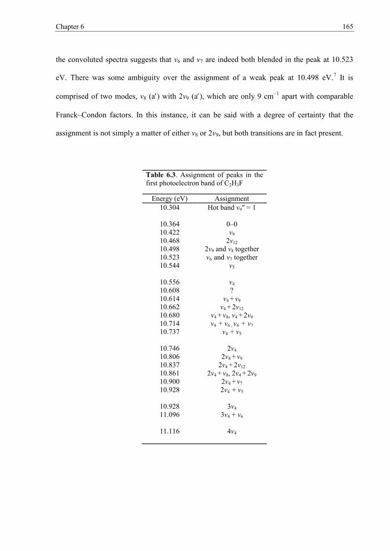
Chapter 6 165

the convoluted spectra suggests that ν6 and ν7 are indeed both blended in the peak at 10.523

eV. There was some ambiguity over the assignment of a weak peak at 10.498 eV.7 It is

comprised of two modes, ν8 (a) with 2ν9 (a), which are only 9 cm–1 apart with comparable

Franck–Condon factors. In this instance, it can be said with a degree of certainty that the

assignment is not simply a matter of either ν8 or 2ν9, but both transitions are in fact present.

Table 6.3. Assignment of peaks in the first photoelectron band of C2H3F

Energy (eV) Assignment 10.304 Hot band ν9″ = 1

10.364 0–0 10.422 ν9 10.468 2ν12 10.498 2ν9 and ν8 together 10.523 ν6 and ν7 together 10.544 ν5

10.556 ν4 10.608 ? 10.614 ν4 + ν9 10.662 ν4 + 2ν12 10.680 ν4 + ν8, ν4 + 2ν9 10.714 ν4 + ν6 , ν4 + ν7 10.737 ν4 + ν5

10.746 2ν4 10.806 2ν4 + ν9 10.837 2ν4 + 2ν12 10.861 2ν4 + ν8, 2ν4 + 2ν9 10.900 2ν4 + ν7 10.928 2ν4 + ν5

10.928 3ν4 11.096 3ν4 + ν6

11.116 4ν4

Chapter 6 166

6.B.1.2. 1,1-Difluoroethene

Figure 6.A(b) shows the TPES of 1,1-C2H2F2 together with the simulated stick and

convoluted spectra. The (2b1)2 HOMO of the C2v neutral means the cation ground state is

2B1. Ab initio calculations show there is a significant increase in the C=C bond length from

1.317 to 1.412 Å upon ionization, and a smaller decrease in the C–F bond length from 1.327

to 1.264 Å. The FCfit analysis results in a small twisting of the CF2 group with respect to the

CH2 group upon ionization (i.e. the dihedral angle of F–C=C–H changes from 180° to 177°),

so the planarity of the molecule is lost in the ground state of the cation. For clarity, C2v

notation is retained the for the vibrational mode symmetries in the cation. Our spectrum

agrees well with both the TPES recorded at lower resolution and the HeI PES recorded at a

comparable resolution by Locht et al.8 The AIE is 10.303 ± 0.005 eV, and the VIE is 10.496 ±

0.005 eV. The major vibrational progression has been assigned to the nv2 (n = 0–6) C=C

stretching mode of a1 symmetry and the peak positions given in Table 6.4 are in excellent

agreement with those of Locht et al.8 Our value for the harmonic frequency ν2 of 1580 cm–1,

obtained from Morse fitting of the progression, is in stunning agreement with the ab initio

value of 1579 cm–1. The anharmonicity constant, xe, is determined to be 0.0046. Three further

minor progressions are also identified and their peak positions are in reasonable agreement

with the HeI study of Locht et al.8 Vibrational assignments are also given in Figure 6.A(b).

For the sake of clarity, the ab initio frequencies, observed frequencies and peak positions are

given in Tables 6.4 and 6.5.

There are several minor peaks sandwiched in between the ν2 peaks of the main

progression. The first one is observed at 10.348 eV and is best assigned to one quantum of ν10

X~

Chapter 6 167

(a2) by FCfit. The experimental value of ν10 = 363 cm–1 is in agreement with the ab initio

result of 373 cm–1. Locht et al. assign this peak to ν9 (b2),8 for which the calculated value of

417 cm–1 is much higher than the experimental value. It applies to both assignments, however,

that these non-totally symmetric vibrations should be forbidden. However, ν10 is seen, albeit

weakly. A possible explanation of how ν10 is observed could be linked to the loss of planar

symmetry upon ionization.

Figure 6.C. The first TPES band of 1,1-C2H2F2 is shown with the Franck–Condon fits including the v5 mode of (a2) symmetry with a calculated B3LYP frequency of 583 cm–1 (red line) v12 mode of (b1) symmetry with a calculated B3LYP frequency of 628 cm–1 (blue line).

Vibronic coupling between the 2B1 and 2B2 states of 1,1-C2H2F2+ which is

mediated by the ν10 (a2) twisting vibrational mode can occur, suggesting a conical intersection

is at play, according to the symmetry requirement;25

X~ A~

Chapter 6 168

(5.3)

This is satisfied with the coupling of the vibronic symmetry of the and states, 2B1 2B2

= A2, giving the symmetry of the vibrational mode, ν10. Therefore, the 2B1 and 2B2 ion states

are coupled when the molecule is twisted, and intensity is given to the ν10 mode upon

ionization. As the predicted torsional angle is only ± 3°, the double-minimum potential energy

curve must be very shallow with the ν10 = 0 and 1 levels most likely above the barrier. In

contrast, the non-adiabatic coupling (via a conical intersection) between the and states

of C2H4+, which is mediated by the torsional mode, produces a torsional angle at the minima

of the ground state which is much larger, ± 29°, with a barrier height of 357 cm–1.19 The

difference in the extent of coupling and therefore the amount of twist seen could be due, in

part, to the larger difference in energy26 between the and states of 1,1-C2H2F2+ of 4.31

eV compared with that of C2H4+ of 2.31 eV.4

The second of these minor peaks at 10.382 eV lies 637 cm–1 above the band origin and

is also well reproduced in the Franck–Condon fitting by the ν12 mode of b1 symmetry at 628

cm–1. This is the only mode within 50 cm–1 of the experimental value of 635 cm–1. Populating

the F–C–F scissor ν5 mode of a1 symmetry, with a frequency of 583 cm–1 gives a similar fit

but it is slightly lower in energy than the ν12 mode (see Figure 6.C). The Franck–Condon

simulation yields a third minor peak at 10.397 eV, which corresponds to a shoulder in the

experimental spectrum at 10.394 eV, assigned as two quanta in the ν10 mode of a2 symmetry

(2×373 cm–1). The difference between the band origin and this shoulder is 0.091 eV or 734

cm–1 which is close to the calculated value of 746 cm–1. This mode becomes allowed under

symmetry considerations even without the breakdown of planarity. Locht et al. do not resolve

this doublet and assign the single peak as 2ν9.8 Even if the HeI peak at 10.347 ± 0.004 eV had

X~ A~

X~ A~

X~ A~

X~ A~

Chapter 6 169

been correctly assigned as ν9 by Locht et al., the 0.042 eV or 338 cm–1 spacing to the 10.389 ±

0.005 eV peak would still mean the latter is unlikely to be 2ν9 with ν9 = 417 cm–1. Note that

both the ν10 and ν12 modes involve a twisting of the CH2 moiety which changes the dihedral

angle, whereas the ν9 mode consists of a F–CC asymmetric in-plane bend (wagging motion)

between the CH2 and CF2 moieties which does not cause a change in this angle. When

populating the ν9 mode instead of either ν10 or ν12, the resulting spectrum is not a satisfactory

fit to the experimental spectra as the H–C=C angle of the cation becomes drastically reduced.

In addition, the experimental spectrum cannot be faithfully reproduced when a planar cation

geometry is retained, confirming that the twist gives rise to the observation of both the ν10 and

ν12 modes.

The fourth peak to high energy of the origin band is at 10.420 eV. This is assigned to

ν4 (a1) = 1, with this FCF symmetric stretching mode at 948 cm–1, to be compared with the

ab initio value of 959 cm–1. Finally, there is a partially resolved shoulder (starting at 10.479

eV) to lower energy of each peak of the main ν2 (a1) progression. Based on the Franck–

Condon simulation, this may correspond to the ν3 (a1) vibrational mode, observed

experimentally at around 1418 cm–1, which can be compared with the ab initio value of 1428

cm–1. This progression was not observed by Locht et al.,8 although the peaks in their ν2

progression do appear to be slightly asymmetric. The same pattern of peaks due to the

vibrational modes ν10, ν12, 2ν10, ν4 and ν3 is repeated for members of the main progression of

nν2 (n = 0–3).

Chapter 6 170

Table 6.4. Calculated (B3LYP) and experimental vibrational modes, symmetries and wavenumbers

( ) of 1,1-C2H2F2 1A1 and 1,1-C2H2F2+ 2B1.

Symmetry 1,1–C2H2F2 1A1 (cm–1)

1,1–C2H2F2+

2B1 (cm–1) Expt

(cm–1)

Description

ν 1 (a1) 3191 3139 C–H symmetric stretch

ν 2 (a1) 1769 1579 a 1580 b C=C stretch, F–C–F symmetric stretch

ν 3 (a1) 1407 1428 a 1419 H–C–H symmetric scissor

ν 4 (a1) 927 959 a 948 C=C stretch, F–C–F symmetric stretch

ν 5 (a1) 546 583 C–F2 scissor

ν 6 (b2) 3292 3268 C–H asymmetric stretch

ν 7 (b2) 1280 1515 F–C–F asymmetric stretch, C–H2 bend

ν8 (b2) 955 1006 H–CC asymmetric bend

ν9 (b2) 438 417 F–CC asymmetric bend

ν10 (a2) 718 373 a 364 C–H2 out-of-plane torsional twist

ν11 (b1) 834 924 Out-of-plane H–C–H rock

ν12 (b1) 624 628 a 635 Out-of-plane C=C rock

a Figures in bold indicate that Franck–Condon activity is observed in these vibrations in the first photoelectron band.

X~ X~

X~ X~

Chapter 6 171

Table 6.5. Assignment of peaks in the first photoelectron band of 1,1-C2H2F2

Energy (eV) Assignment

10.260 Hot band

10.303 0–0 10.348 ν10 10.382 ν12 10.394 2ν10 10.420 ν4 10.456 10.479 ν3

10.496 ν2 10.542 ν2 + ν10 10.577 ν2 + ν12 10.590 ν2 + 2ν10 10.610 ν2 + ν4 10.651 10.675 ν2 + ν3

10.690 2ν2 10.734 2ν2 + ν10 10.768 2ν2 + ν12 10.779 2ν2 + 2ν10 10.803 2ν2 + ν4 10.847 2ν2 + ν3

10.882 3ν2 10.925 3ν2 + ν10 10.958 3ν2 + ν12 10.975 3ν2 + 2ν10 11.000 3ν2 + ν4 11.034 3ν2 + ν3

11.069 4ν2 11.111 4ν2 + ν10 11.148 4ν2 + ν12

11.257 5ν2

Chapter 6 172

6.B.1.3. Trifluoroethene

Figure 6.D(a) shows the TPES of C2HF3, the simulated stick and convoluted spectra

together with the vibrational assignments. Although some vibrational structure has been

observed in the ground-state PE band by others,2,4 this is the first high resolution TPES of this

molecule reported in the literature. The (4a″)2 HOMO of the neutral CS C2HF3 molecule has

C=C π orbital character, and the cation electronic ground state has the term symbol 2A″.

Similarly with the previous fluorinated ethenes, ab initio calculations show an increase in the

C=C bond length from 1.323 to 1.418 Å consistent with removing an electron from the C=C π

orbital, and a decrease in all C–F bond lengths of ≈ 0.06 Å. The geometry obtained from FCfit

shows planarity is retained within the ion.

The first photoelectron band, corresponding to the 2A″ ground state of C2HF3+ is

comprised of a series of sharp and well defined peaks. The AIE and VIE are 10.138 ± 0.007

and 10.544 ± 0.007 eV, respectively. Previous literature values are scarce with the notable

exception of the work by Bieri et al., who reported the AIE as 10.14 eV and the VIE as 10.62

eV,2 both in close agreement with the values of this work. The band is dominated by a

vibrational progression of nν2 mode (n = 0–5) which corresponds to the C=C stretching mode.

The Morse-fitted vibrational harmonic frequency of this band is determined to be 1641 cm–1,

which is in close agreement with the ab initio value of 1649 cm–1.

X~

X~

Chapter 6 173

Figure 6.D. The first TPES band of (a) C2HF3 and (b) C2F4 is shown with the Franck–Condon stick (blue stick) simulations and convoluted curve (blue curves). Reassignments of vibrational modes are indicated by square brackets.

Chapter 6 174

The anharmonicity constant, xe, is determined to be 0.000781. This assignment is in

agreement with the early angle-resolved photoelectron spectrum of Sell and Kuppermann4

(Tables 6.6 and 6.7 ). There are five other, less intense vibrational progressions amidst

members of the ν2 progression. With the aid of FCfit, they are assigned to ν9 (C–H in plane

rock and CC–F bend) at 241 cm–1, ν8 (Fa–C1C2 scissor, where Fa is cis to the hydrogen) at 508

cm–1, ν7 (F–CC scissor and Fb–CC scissor where Fb is trans to the hydrogen) at 629 cm–1, ν5

(C–H wag) at 1266 cm–1, and ν4 (F–C2 stretch, H–CC bend and C1–Fa stretch) at 1654 cm–1.

The overall agreement between experiment and fit is excellent. Figure 6.B shows the

calculated and experimental vibrational modes which are active upon ionization and their

symmetries. All six active modes are of a′ symmetry and satisfy selection rules. Furthermore,

just as for monofluoroethene with CS symmetry, no single quantum of a vibrational modes

are observed, consistent with a planar cation. Unlike in monofluoroethene, double quanta of

a modes are not observed in trifluoroethene either. The same pattern of peaks due to the

vibrational modes ν9, ν8, ν7, ν5 and ν4 is observed toward higher energy from the main

progression peaks nν2 (n = 0–4).

Chapter 6 175

Table 6.6. Calculated (B3LYP) and experimental vibrational modes, symmetries and wavenumbers ( ) of C2HF3 1A′ and C2HF3

+ 2A″.

Symmetry C2HF3 1A′ (cm–1)

C2HF3+

2A″ (cm–1) Expt

(cm–1)

Description

ν1 (a′) 3252 3186 C–H stretch

ν 2 (a′) 1824 1649 1641 b C=C stretch

ν 3 (a′) 1352 1535 Fa–C1–Fb asymmetric stretch, C–H wag

ν 4 (a′) 1251 1387 1654 C–H wag, Fa–C1–Fb asymmetric stretch,

ν 5 (a′) 1160 1281 1266 F–C2 stretch

ν 6 (a′) 933 952 C–H wag, Fa–C1–Fb symmetric stretch

ν 7 (a′) 621 648 629 F–CC scissor, Fb–CC scissor

ν 8 (a′) 483 491 508 Fa–C1–C2 scissor

ν 9 (a′) 233 240 241 C–H in plane rock, CF2 bend

ν 10 (a″) 782 812 Out-of-plane C–H rock

ν 11 (a″) 575 578 Out-of-plane C–C–H rock

ν 12 (a″) 306 223 Out-of-plane H rock

a Figures in bold indicate that Franck–Condon activity is observed in these vibrations in the first photoelectron band. b Harmonic frequency derived by Morse fitting of the vibrational progression (see text).

X~ X~

X~ X~

Chapter 6 176

Table 6.7. Assignment of peaks in the first photoelectron band of C2HF3


10.073 Hot band 10.097 Hot band 10.108 Hot/sequence band

10.138 0–0 10.168 ν9 10.201 ν8 10.216 ν7 10.295 ν5 10.331 ν4

10.342 ν2 10.373 ν2 + ν9 10.407 ν2 + ν8 10.418 ν2 + ν7 10.499 ν2 + ν5 10.519 ν2 + ν4

10.544 2ν2 10.576 2ν2 + ν9 10.605 2ν2 + ν8 10.619 2ν2 + ν7 10.702 2ν2 + ν5 10.726 2ν2 + ν4

10.746 3ν2 10.778 3ν2 + ν9 10.809 3ν2 + ν8 10.822 3ν2 + ν7 10.901 3ν2 + ν5 10.927 3ν2 + ν4

10.949 4ν2 10.978 4ν2 + ν9 11.011 4ν2 + ν8 11.021 4ν2 + ν7 11.101 4ν2 + ν5 11.127 4ν2 + ν4

11.146 5ν2

Chapter 6 177

6.B.1.4. Tetrafluoroethene

C2F4 has the highest symmetry of the four molecules studied, belonging to the D2h

point group. The HOMO of the neutral is the C=C π bonding orbital, (2b3u)2, and the cation

ground state has the term symbol 2B3u.2 Using FCfit, the ground state geometry of the

cation is confirmed to be planar, and only totally symmetric vibrations in the D2h point group

should be observed in the photoelectron spectrum with the highest intensity. As previously,

there is an increase in the C=C bond length of 0.096 Å, a decrease in the C–F bond length of

0.056 Å. Overall across the series, the increase in C=C bond length upon ionization becomes

greater with increasing F-substitution, but the decrease in C–F bond length is reduced, in

accordance with the perfluoro effect, i.e. σ molecular orbitals are strongly stabilized by

mixing of the ethylene group orbitals with the electronegative F-atom σ orbitals. By contrast,

the mixing and stabilization of the π orbitals is much smaller and so strong C–F π anti-

bonding character dominates.3

The first photoelectron band seen in Figure 6.D(b) is assigned to the ground state of

C2F4+, 2B3u. It is composed of several well-defined vibrational progressions, the most

prominent being the nν1 (n = 0–7), the C=C stretching mode at 1708 cm–1, in good agreement

with the experimental value from the Morse-fitted progression of 1733 cm–1. The

anharmonicity constant, xe, is determined to be 0.00366. The calculated and experimental

frequencies are given in Figure 6.B. The AIE and VIE are 10.110 ± 0.009 and 10.535 ± 0.009

eV, respectively. Five additional but less intense vibrational progressions are in between the

members of the ν1 progression. Three have been assigned as ν3, ν2 and (ν3 + ν2), with

X~

X~

Chapter 6 178

experimental frequencies of 468, 847 and 1315 cm–1 respectively (see Figure 6.D(b)) and, as

expected, all identified modes are of ag symmetry (Tables 6.8 and 6.9).

In an earlier lower resolution TPE study by Jarvis et al.,9 only the ν1, ν2 and ν3 modes

were observed (note that the numbering of ν1 and ν2 is reversed in both the Jarvis et al. and

Brundle et al. studies).3 Following a subtraction procedure to allow for the effects of second-

order harmonic radiation delivered from the grating monochromator at the beamline, Jarvis et

al. determined the AIE to be 10.0 ± 0.1 eV, and the vibrational frequencies of these three

modes to be 1686, 766 and 371 cm–1,9 in reasonable agreement with those determined from

the present work of 1733, 847 and 468 cm–1, respectively. The ground state of C2F4+ was also

studied by HeI photoelectron spectroscopy at a resolution of 0.022 eV by Eden et al.10 The

first and third progressions were also identified by Eden et al. as ν1 (C=C stretch) and ν2 (C=C

stretch and C–F2 symmetric stretch).10 However, there is disagreement between the

assignment of the second and fourth progression, which they assign by comparison with the

infrared spectrum of neutral C2F4, as the ν6 mode of b1g symmetry and the ν11 mode of b3u

symmetry using the Herzberg convention.27 In the Mulliken convention used here, these

vibrations are the ν11 (b3g) CC–F bend and ν5 (b1u) symmetric C–F2 stretch modes.28 Since

there is no change in the molecular symmetry, odd-quantum transitions are only allowed for

totally symmetric modes. Therefore, the Eden assignments are disputed and reassignment of

modes with b3g and b1u symmetry in favour of a combination band assignment where both

modes have ag symmetry are recommended. Consequently, these bands have been reassigned

as the ν3 mode and the combination band (ν3 + ν2), respectively. The average spacing between

the second of the two peaks from the main progression is reported by Eden as 0.152 eV or

1225 cm–1 and assigned to ν11.10 However, the average difference in this work between this

progression and the corresponding members of the ν1 progression is 1245 cm–1, but the

Chapter 6 179

difference between the band origin and the first member of this progression at 10.273 eV is

0.163 eV or 1315 cm–1. This second value is least affected by anharmonicity and is preferred

over the average value.It is also in excellent agreement with the sum of the experimental

values for ν3 + ν2, 1315 cm–1.

Thanks to the enhanced resolution, an additional, previously unobserved progression

has been identified with two peaks in each member of the main progression with a spacing of

637 and 1008 cm–1 from the band origin. This progression with members at 10.188 and

10.235 eV is well reproduced when populating the ν6 mode (C–F2 scissor out of

synchronicity) of b1u symmetry with one and two quanta. Both the ν6 mode and the other

possibility, ν9 of b2u symmetry, are non-totally symmetric, so should be forbidden transitions

in the absence of a geometry change upon ionization. Yet by evaluating the actual nuclear

wave function overlap, Franck–Condon simulations show that ν6 is populated with non-

negligible intensity even without a change in symmetry. Finally, the same pattern of peaks at

ν2, ν6, ν3, 2ν6 and (ν2 + ν3) is repeated for each member of nν1 (n = 0–6).

It appears that with the exception of 1,1-C2H2F2+, the rest of the series, C2H3F+,

C2HF3+ and C2F4

+ remain planar upon ionization in the ground electronic cation state. The

experimental spectra cannot be faithfully reproduced with a non-planar ion geometry in these

latter three ions. Apparently, the vibronic coupling between the π(C=C) and π(C–X2) where X

= H or F,26 is only measurable in 1,1-C2H2F2+, in which a torsional twist is observed.

A final note upon the TPES of the ground electronic states of the four fluorinated

ethenes presented in this work is made. The successful application of fitting the ground state

band with the Franck–Condon intensities and apparent similarities between the PES2,4,7,8 and

TPES of this work indicates that no autoionization effects are seen.

Chapter 6 180

Table 6.8. Calculated (B3LYP) vibrational modes, symmetries and wavenumbers ( ) of C2F4 1Ag and C2F4

+ 2B3u.

Symmetry† C2F4 1Ag

(cm–1) C2F4

+ 2B3u (cm–1)

Expt Value (cm–1)

Description

ν1 (ag) 1908 1708 b 1733 c C=C stretch

ν2 (ag) 788 832 b 847 C=C stretch, symmetric C–F2 stretch

ν3 (ag) 397 407 b 468 C=C stretch, symmetric C–F2 scissor

ν4 (au) 198 140 CF2 torsional twist

ν5 (b1u) 1173 1275 Symmetric C–F2 stretch, (out of synchronicity)

ν6 (b1u) 551 603 b 637 CC–F bend (out of synchronicity)

ν7 (b2g) 556 599 Out-of-plane C=C umbrella mode

ν8 (b2u) 1312 1536 Asymmetric C–F2 stretch (in synchronicity)

ν9 (b2u) 211 215 CC–F bend

ν10 (b3g) 1310 1532 Asymmetric C–F2 stretch, (out of synchronicity)

ν11 (b3g) 550 536 CC–F bend

ν 12 (b3u) 414 438 Out-of-plane C=C umbrella mode a The labelling of v1 and v2 is reversed from the nomenclature used by Jarvis et al.9b Figures in bold indicate that Franck–Condon activity is observed in these vibrations in the first photoelectron band. c

Harmonic frequency derived by Morse fitting of the vibrational progression (see text).

†Note the Mulliken convention is used throughout this work, where the z-axis is along the C=C bond and the x-axis is perpendicular to the molecular plane. The Herzberg convention as used by Eden et al.8 has the x-axis along the C=C bond and the z-axis perpendicular to the molecular plane.

X~

X~

X~ X~

Chapter 6 181

Table 6.9. Assignment of peaks in the first photoelectron band of C2F4


10.504 Hot/sequence band 10.110 0–0

10.168 ν3 10.188 ν6 10.215 ν2 10.235 2ν6 10.273 ν3 + ν2

10.326 ν1 10.378 ν1 + ν3 10.396 ν1 + ν6 10.427 ν1 + ν2 10.451 ν1 + 2ν6 10.482 ν1+ ν3 + ν2

10.535 2ν1 10.592 2ν1 + ν3 10.606 2ν1 +ν6 10.639 2ν1 + ν2 10.658 2ν1 +2ν6 10.695 2ν1 + ν3+ ν2

10.746 3ν1 10.800 3ν1 + ν3 10.815 3ν1 + ν6 10.847 3ν1 + ν2 10.872 3ν1 + 2ν6 10.899 3ν1 + ν3+ ν2

10.954 4ν1 11.007 4ν1 + ν3 11.016 4ν1 + ν6 11.054 4ν1 + ν2 11.095 4ν1 + ν3+ ν2

11.159 5ν1 11.223 5ν1 + ν3 11.273 5ν1 + ν2

11.364 6ν1 11.435 6ν1 + ν3

11.570 7ν1

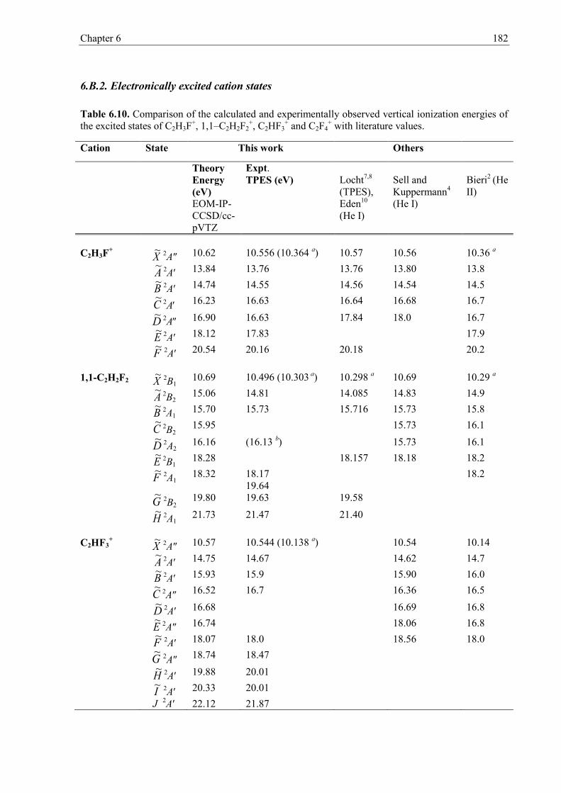
Chapter 6 182

6.B.2. Electronically excited cation states

Table 6.10. Comparison of the calculated and experimentally observed vertical ionization energies of the excited states of C2H3F+, 1,1–C2H2F2

+, C2HF3+ and C2F4

+ with literature values.

Cation State This work Others

Theory Energy (eV) EOM-IP-CCSD/cc-pVTZ

Expt. TPES (eV)

Locht7,8 (TPES), Eden10 (He I)

Sell and Kuppermann4 (He I)

Bieri2 (He II)

C2H3F+ 2A″ 10.62 10.556 (10.364 a) 10.57 10.56 10.36 a

2A′ 13.84 13.76 13.76 13.80 13.8 2A′ 14.74 14.55 14.56 14.54 14.5 2A 16.23 16.63 16.64 16.68 16.7 2A 16.90 16.63 17.84 18.0 16.7 2A′ 18.12 17.83 17.9 2A′ 20.54 20.16 20.18 20.2 1,1-C2H2F2 2B1 10.69 10.496 (10.303 a) 10.298 a 10.69 10.29 a 2B2

15.06 14.81 14.085 14.83 14.9 2A1

15.70 15.73 15.716 15.73 15.8 2B2

15.95 15.73 16.1 2A2

16.16 (16.13 b) 15.73 16.1 2B1

18.28 18.157 18.18 18.2 2A1

18.32 18.17 19.64

18.2

2B2 19.80 19.63 19.58 2A1 21.73 21.47 21.40 C2HF3

+ 2A″ 10.57 10.544 (10.138 a) 10.54 10.14

2A′ 14.75 14.67 14.62 14.7 2A′ 15.93 15.9 15.90 16.0 2A″ 16.52 16.7 16.36 16.5 2A′ 16.68 16.69 16.8 2A″ 16.74 18.06 16.8 2A′ 18.07 18.0 18.56 18.0 2A″ 18.74 18.47 2A′ 19.88 20.01 2A′ 20.33 20.01 J 2A′ 22.12 21.87

X~

A~

B~

C~

D~

E~

F~

X~

A~

B~

C~

D~

E~

F~

G~

H~

X~

A~

B~

C~

D~

E~

F~

G~

H~

I~

Chapter 6 183

Theory Energy (eV) EOM-IP-CCSD/cc-pVTZ

Expt. TPES (eV)

Locht7,8 (TPES), Eden10 (He I)

Sell and Kuppermann4 (He I)

Bieri2 (He II)

C2F4

+ 2B3u 10.60 10.535 (10.110 a) 15.93 c 10.56 10.14 2B3g

15.96 15.99 15.95 15.9 2Ag

16.33 16.20 16.64 c 16.63 16.6 2B2u

16.50 16.56 16.64 c 16.63 16.6 2Au

16.86 16.92 16.64 c 16.63 16.6 2B1g

17.53 17.62 16.64 c 16.6 2B2u

18.21 18.41 17.60 c 17.60 17.6 2B2g 19.43 19.48 18.2 2B3u 19.57 19.48 19.4 2B3g 20.93 21.05 19.4 J 2B2u 21.26 21.05 21.0 K 2Ag 22.59 22.55 21.0 a Adiabatic IE. b Shoulder. c Eden et al.10

6.B.2.1. Spectroscopy

Equation-of-motion coupled cluster singles and doubles for ionized states, EOM-IP-

CCSD/cc-pVTZ calculations29 were undertaken using Q-Chem 3.230 at the optimized G3B3

neutral geometries to determine accurate vertical ionization energies and assign excited

electronic state TPES bands, the results are given in Table 6.10. Excited state wave functions

of the cation are of single determinant character and Koopmans’ theorem31 holds. Thus, the

EOM-IP-CCSD assignment agrees exactly with the semi-empirical HAM/3-based ordering of

the cations published thirty years ago by Bieri et al.2 and, with the exception of the almost

degenerate , and , electronic states in 1,1-C2H2F2+ and C2F4

+, respectively, also

with their Green’s function analysis. Counter-intuitively, electronic excited state assignments

are straightforward for the fluorinated ethene ions with little static electron correlation, in

X~

A~

B~

C~

D~

E~

F~

G~

H~

I~

E~ F~ H~ I~

Chapter 6 184

sharp contrast with the vibrational assignments of the ground state spectra, where it has been

found that even the most recent vibrational assignments need revision.7,8,10

Figure 6.E. Complete valence threshold photoelectron spectra of C2H3F, 1,1-C2H2F2, C2HF3 and C2F4. The EOM-IP-CCSD/cc-pVTZ computed vertical ionization energies are shown by the symbols. Different symbols represent different ion states according to their (approximate, see text) C2v character: A1 (black triangle), A2 (light circle), B1 (black circle), B2 (light triangle).

Chapter 6 185

Two of the molecules studied, C2H3F and C2HF3, have CS symmetry, 1,1-C2H2F2 has

C2v and C2F4 has D2h symmetry. In order to establish trends and trace the evolution of the

electronic ion states in the series, the Kohn–Sham orbital character symmetries according to

their C2v character were considered, even for the CS molecules, as follows. Orbitals without a

nodal plane along the C=C axis are classified as totally symmetric, giving the corresponding

ion state A1 symmetry. Ionization from orbitals with a nodal plane in the molecular plane but

without one perpendicular to it leads to B1 ion states. Orbitals with a nodal plane

perpendicular to the molecular plane along the C=C axis correspond to B2 ion states. When

both nodal planes are present in orbitals, ionization leads to A2 states. This assignment is

shown together with the overall TPES in Figure 6.E. The slight destabilization of the π-type

HOMO corresponding to the ground ion state and the overall stabilization of the deeper lying

orbitals, i.e. progressively higher ionization energies corresponding to excited ion states, with

increasing F substitution confirms not only the perfluoro effect,3 but also the enhanced

stabilization of the fluorine lone pairs. With the exception of this point, other trends with

increasing fluorine substitution are difficult to establish.

Vibrational progressions have been observed in some excited states in all four

molecules. When vibrational structure is observed in the excited states, Franck–Condon

factors have to be significant for levels in the bottom of the potential energy well, and it can

be assumed that the geometries of the excited state ion are comparable to that of the ground

neutral state. Within this approximation, only tentative assignments based on the ion ground

state calculated frequencies can be made. A strong well-resolved progression is seen on the

2A′ state of C2HF3+ between 19.4 and 20.3 eV which has not been previously reported. The

observed spacing of ca. 847 cm–1 could be attributed to an asymmetric wagging mode with a

Fa–C1Fb symmetric stretch, or even quanta of a Fa–C1=C2 bending mode. There is very weak

H~

Chapter 6 186

vibrational structure seen between 22.5–24.9 eV with a separation of ca. 240 cm–1, which

could be attributed to the CHF=CF2 wagging mode. The strongest vibrational structure in the

excited states of C2F4+

is seen on the 2B1g peak at 17.6 eV, also observed in the HeI spectra

of Brundle et al.3 and Eden et al.10 Brundle et al. assign the complex structure to two separate

progressions, ν2 and ν3.3 The ν2 mode involving the C=C stretch, makes a more likely

candidate for the major progression where a vibrational spacing of ca. 777 cm–1 rather than

the ν11 mode (calculated at 536 cm–1 in the ground cation state) proposed by Eden et al is

observed.10 The minor progression has an observed vibrational spacing of ca. 398 cm–1 and is

assigned to the ν3 mode, a C=C stretch with symmetric C–F2 scissor, in accordance with

Brundle et al.3 A final single vibrational progression is seen on the peak at 19.1–19.7 eV

(ionic states with 2B2g and 2B3u symmetry) and is assigned to the ν2 mode, ca. 777 cm–1,

again in accordance with Brundle et al.3 Locht et al.7,8 reported a large intensity ratio for the

excited vs. ground electronic state bands in the TPES, whereas in this chapter, it is found that

the ground state bands have comparable intensities to the first excited state band in the TPES.

This could be due to disparities between how the photon flux is accounted for.

6.B.2.2. Dynamics

The dissociative photoionization dynamics is of both applied and fundamental

interest.32 On the one hand, appearance energies can be used in thermochemical derivations,

but only if the dissociative photoionization is fast at the thermochemical threshold33 or if the

dissociation rates can be measured and extrapolated to it.34 In addition to new and accurate

neutral thermochemistry, such thresholds can also help interpret the products of ion-molecule

bimolecular reactions.35 On the other hand, understanding the energy flow between different

E~

G~ H~

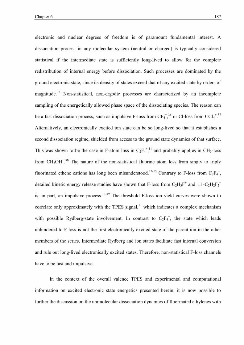
Chapter 6 187

electronic and nuclear degrees of freedom is of paramount fundamental interest. A

dissociation process in any molecular system (neutral or charged) is typically considered

statistical if the intermediate state is sufficiently long-lived to allow for the complete

redistribution of internal energy before dissociation. Such processes are dominated by the

ground electronic state, since its density of states exceed that of any excited state by orders of

magnitude.32 Non-statistical, non-ergodic processes are characterized by an incomplete

sampling of the energetically allowed phase space of the dissociating species. The reason can

be a fast dissociation process, such as impulsive F-loss from CF4+,36 or Cl-loss from CCl4

+.37

Alternatively, an electronically excited ion state can be so long-lived so that it establishes a

second dissociation regime, shielded from access to the ground state dynamics of that surface.

This was shown to be the case in F-atom loss in C2F4+,11 and probably applies in CH3-loss

from CH3OH+.38 The nature of the non-statistical fluorine atom loss from singly to triply

fluorinated ethene cations has long been misunderstood.12-15 Contrary to F-loss from C2F4+,

detailed kinetic energy release studies have shown that F-loss from C2H3F+ and 1,1-C2H2F2+

is, in part, an impulsive process.13,39 The threshold F-loss ion yield curves were shown to

correlate only approximately with the TPES signal,11 which indicates a complex mechanism

with possible Rydberg-state involvement. In contrast to C2F4+, the state which leads

unhindered to F-loss is not the first electronically excited state of the parent ion in the other

members of the series. Intermediate Rydberg and ion states facilitate fast internal conversion

and rule out long-lived electronically excited states. Therefore, non-statistical F-loss channels

have to be fast and impulsive.

In the context of the overall valence TPES and experimental and computational

information on excited electronic state energetics presented herein, it is now possible to

further the discussion on the unimolecular dissociation dynamics of fluorinated ethylenes with

Chapter 6 188

respect to a previous study (see Chapter 5).11 Out of computational practicality, only the

dissociation mechanism of monofluoroethene cations is considered, using EOM-IP-CCSD/cc-

pVTZ calculations along the optimized11 cation ground electronic state H-, HF- and F-loss

reaction paths. That is, the reaction path geometries are optimized at the B3LYP/6-

311++G(d,p) level on the ground cation state, and vertical excitations are considered to the

electronically excited states. Because of the spectral similarity, an analogous mechanism is

expected to apply to the dissociation dynamics of di- and trifluoroethene cations. By contrast,

the spectral sparsity of the TPES of tetrafluoroethene leads to a de-coupling of the ion state

from the ion state, leading to isolated-state behaviour with long-lived state

intermediates.11 By understanding the role of different electronically excited ion states in the

mechanism of the main dissociative photoionization channels, it will be shown how and why

F-atom loss assumes a non-statistical character in higher internal energy states of the parent

ions, whereas the HF- and H-loss channels do not.

6.B.2.1 H-atom loss from C2H3F+

The H-loss reaction energy curves in the monofluoroethene cation are shown in Figure

6.F. The doublet ground ion state is of A″ symmetry. The molecular orbital of the missing

electron in the dominant electron configuration of the cation in the first four electronic states

is also shown in the figure, together with that in the electronic ground state of the ion, at a C–

F bond length of 2.9 Å. The F atom is pointing out of the plane towards the reader in the

schematic structures. The ground state of the H-loss fragment ion, CH2=CF+, is closed shell,

i.e. totally symmetric (A′) in CS symmetry and the spin density is localized in the 1s orbital of

the leaving H atom in the products.

A~

X~ A~

Chapter 6 189

Figure 6.F. Reaction curves of the , , and excited states of C2H3F+ along the H-loss coordinate in the ground state ion. Conical intersections (indicated as funnels) are indicated at R(C–H)

≈ 2.05 Å between the and states, and at R(C–H) ≈ 2.1 Å between the and states.

In other words, the state of the parent ion adiabatically correlates with the CH2=CF∙+ H+

dissociation products, but H+ is not observed in the valence photoionization

experiments.11The thermochemical threshold to H-atom loss is 13.6 eV.11 In order to

determine the well depth of the state, which can indeed correlate adiabatically with the H-

loss products, an EOM-IP-CCSD geometry optimization was carried out, that yielded a

structure with an elongated α-C–H bond length and increased C–C–F bond angle as well as an

adiabatic ionization energy of 13.18 eV. Therefore, the state of C2H3F+ is bound by ≈ 400

meV, it adiabatically correlates with the ground state H-loss products, and is coupled with the

X~ A~ B~ C~

X~ A~ B~ C~

X~

A~

A~

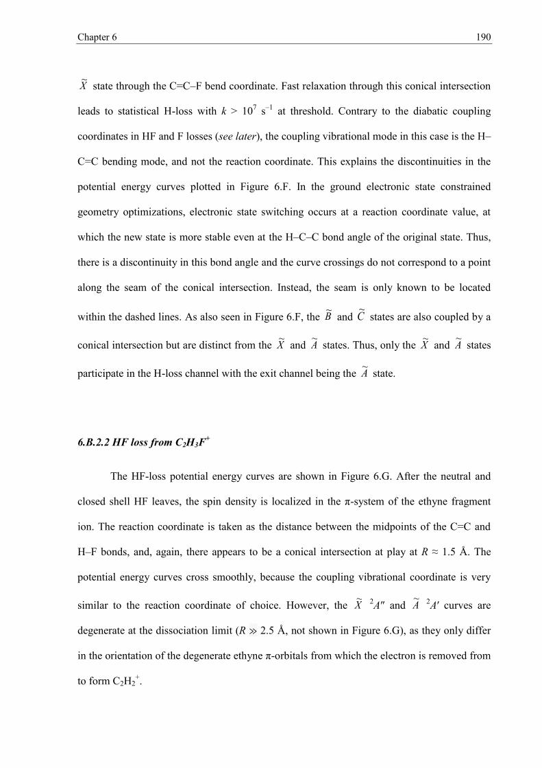
Chapter 6 190

state through the C=C–F bend coordinate. Fast relaxation through this conical intersection

leads to statistical H-loss with k > 107 s–1 at threshold. Contrary to the diabatic coupling

coordinates in HF and F losses (see later), the coupling vibrational mode in this case is the H–

C=C bending mode, and not the reaction coordinate. This explains the discontinuities in the

potential energy curves plotted in Figure 6.F. In the ground electronic state constrained

geometry optimizations, electronic state switching occurs at a reaction coordinate value, at

which the new state is more stable even at the H–C–C bond angle of the original state. Thus,

there is a discontinuity in this bond angle and the curve crossings do not correspond to a point

along the seam of the conical intersection. Instead, the seam is only known to be located

within the dashed lines. As also seen in Figure 6.F, the and states are also coupled by a

conical intersection but are distinct from the and states. Thus, only the and states

participate in the H-loss channel with the exit channel being the state.

6.B.2.2 HF loss from C2H3F+

The HF-loss potential energy curves are shown in Figure 6.G. After the neutral and

closed shell HF leaves, the spin density is localized in the π-system of the ethyne fragment

ion. The reaction coordinate is taken as the distance between the midpoints of the C=C and

H–F bonds, and, again, there appears to be a conical intersection at play at R ≈ 1.5 Å. The

potential energy curves cross smoothly, because the coupling vibrational coordinate is very

similar to the reaction coordinate of choice. However, the 2A″ and 2A′ curves are

degenerate at the dissociation limit (R ≫ 2.5 Å, not shown in Figure 6.G), as they only differ

in the orientation of the degenerate ethyne π-orbitals from which the electron is removed from

to form C2H2+.

X~

B~ C~

X~ A~ X~ A~

A~

X~ A~

Chapter 6 191

Figure 6.G. Reaction curves of the , , and excited states of C2H3F+ along the HF-loss coordinate. A conical intersection has been located at R(C•C–H•F) ≈ 1.5 Å.

As one approaches the products, the (HOMO–1) of the neutral takes a σ-antibonding

character between the fragments, whereas the HOMO corresponds to a π-antibonding orbital.

Thus at R = 2 Å, the A′ state of the cation with one σ-antibonding electron removed is more

stable than the A″ state ion (see schematic structures in the figure with the corresponding

molecular orbitals in the neutral at the highlighted reaction coordinate with the HF leaving

upwards). The energy difference between the two states is larger than 0.5 eV when HF is

removed by 2.5 Å from C2H2+, showing a long range interaction at play. The 2A′ state of

C2H3F+ correlates with the ground state C2H2 + HF+ products, lying 5 eV above the lower

X~ A~ B~ C~

B~

Chapter 6 192

energy and channels, the corresponding molecular orbital of the missing electron being

of F lone pair character, as shown. On the state surface, the transition state to HF loss lies

20 eV above the neutral, and is even higher for the and ( state not shown) states

which correlate with excited state products. As was the case for H loss, HF loss in C2H3F+ is

related by the interplay between the and states. Higher-lying ion states are de-coupled

from the HF-loss channel observed in dissociative valence photoionization, as they must first

relax to the / manifold in order to lose HF in a statistical fashion.

6.B.2.3. F-atom loss from C2H3F+

The F-loss potential energy curves, shown in Figure 6.H, show a different pattern. The

first three ion states, , and , dissociate to products with different singly occupied

fluorine 2px,y,z orbitals and the same ground electronic state of the CH2CH+ ion. At a fluorine–

carbon distance of around R(C–F) = 2.3 Å, the three states are degenerate and are coupled by

the C–F stretch coordinate. At longer distances, the state appears to be converged to the

dissociation limit, whereas even at R = 3.3 Å, the and states increase in energy. This

suggests that long range interactions are significant at even longer distances than for HF-loss,

as there has to be an / F-loss transition state at R(C–F) > 3.3 Å. To describe this bond

length region reliably, the triple-ζ basis set used in these calculations would need to be

augmented with several diffuse functions.

X~ A~

B~

C~ D~ D~

X~ A~

X~ A~

X~ A~ B~

B~

X~ A~

X~ A~

Chapter 6 193

Figure 6.H. Reaction curves of the , , and excited states of C2H3F+ along the F-loss

coordinate. Three conical intersections have been found R(C–F) ≈ 1.5 Å between and , R(C–F)

≈ 1.8 Å between and and at R(C–F) ≈ 2.3 Å between the , , and states leading to degenerate asymptotes.

The non-statistical F-loss process arises in the energy range of the 2A″ state. Based

on the low energy component in the kinetic energy release distribution and ab initio

calculations, the dissociation channel from this state to the C2H3+ (3A″) + F (2P) products

was suggested to play an important role.7,14,15 Rooda et al.15 further established that the

state has a large negative energy gradient towards the C–F elongation, and suggested a

diabatic pathway in which the and states couple through an avoided crossing at R(C–F)

= 2.0 Å with a minimum energy gap of around 0.96 eV. Their proposed route to F-atom

X~ A~ B~ C~

C~ B~

B~ C~ X~ A~ B~

C~

C~

C~

C~ X~

Chapter 6 194

formation is either via this diabatic pathway along which the initial momentum in the C–F

stretch is retained, leading to ground state C2H3+ (1A′) with a large translational kinetic energy

release, or via an adiabatic pathway along the state producing electronically excited triplet

C2H3+ (3A″) fragment ion with small kinetic energy release. The fragments of the latter

channel, however, correspond to a quartet wave function, meaning that it cannot be the

asymptote of the doublet state. Indeed, it was found that the 4A″ quartet state crosses the

2A″ state at R(C–F) ≈ 2.2 Å (Figure 6.H). The rate of the intersystem crossing is, however,

unlikely to exceed that of internal conversion to lower lying doublet ion states. The

breakdown diagram11 casts further doubt on the feasibility of this pathway. The CBS-APNO40

calculated splitting between the singlet and triplet states of the vinyl cation is 2.10 eV, putting

the asymptote to triplet C2H3+ production at ≈ 16.1 eV (cf. the 16.6 eV limit in Fig. 6.H

corresponding to the triplet energy at the singlet C2H3+ product geometry, calculated using

EOM-IP-CCSD/cc-pVTZ). In the breakdown diagram of C2H3F+,11 the percentage yield of F-

loss production plateaus at ≈30% in the statistical regime, then rises rapidly in the photon

energy region 15.5–16 eV to a constant level of ≈60% from which the signal decreases above

a photon energy of 17.0 eV. If triplet C2H3+ production were a viable dissociation path, the F-

loss signal should increase above its threshold at 16.1 eV, at which energy it has already

reached its asymptotic value. The absence of such an increase rules out significant C2H3+

(3A″) production and an alternative mechanism is offered below.

As opposed to the , and states, the state of C2H3F+ converges to CH2CH +

F+, and does not lead to F-loss products. However, it is just below the onset of this excited A″

ion state peak in the threshold photoelectron spectrum11 that the non-statistical and partly

impulsive13 F-loss channel opens up. Figure 6.H shows that the and states are coupled

C~

C~ C~

X~ A~ B~ C~

B~ C~

Chapter 6 195

at 1.5 Å < R(C–F) < 1.8 Å. As Rooda et al. have shown,15 the C–F bond length in the state

minimum is markedly longer than in the ground state of the ion, thanks to the removal of an

electron from a π-type C–F bonding orbital in ionization to the ion state. Consequently,

state ions are highly vibrationally excited in the Franck–Condon envelope with large

excitation in modes associated with the C–F stretch. state ions can lose electronic

excitation energy by crossing through the conical intersections to the state. If the crossing

occurs at low C–F bond lengths on the bound part of the surface, the resulting species will

decay statistically. However, at higher C–F bond lengths, the state also has a repulsive

character that facilitates F-atom loss. The fate of the parent cation is still not sealed at this

point, since fluorine p-orbital mixing at R(C–F) = 2.3 Å can lead it onto the partially bound

and states, yielding a longer lived F-loss intermediate, in which redistribution of the excess

energy may, to a certain extent, still be possible. Thus, three different F-loss channels are

proposed in the state band of the TPES of C2H3F: (i) statistical F-loss mostly from the

state by a → transition on the bound part of the state surface, through the first

conical intersection, (ii) impulsive F-loss by a → transition onto the repulsive part of

the state and subsequent direct dissociation, and, as a slight variation of this process, (iii)

semi-impulsive non-statistical F-loss by a multi-step → → / transition with an

intermediate at R(C–F) ≈ 2.3 Å.

This multiple channel F-loss mechanism explains the proposed bimodal kinetic energy

release distribution observed for C2H3F+ and 1,1-C2F2H2+,14,15,39 as the low kinetic energy

release modus is a result of the statistical dissociation pathway. Furthermore, direct -state

involvement is not necessarily required in threshold photoionization. As was proposed in the

C~

C~ C~

C~

B~

B~

B~

A~

X~

C~ X~

C~ B~ B~

C~ B~

B~

C~ B~ X~ A~

C~

Chapter 6 196

study of CH3I,23 the neutral parent can be excited to the Rydberg manifold in the initial step.

The Rydberg manifolds belonging to each ion state will have the similar characteristics to the

ion state, and autoionization may also occur after internal conversion. This explains why the

non-statistical F-loss channel is seen at slightly lower energies than the actual -state peak in

the photoelectron spectrum of C2H3F+. In the iodomethane study,23 neutral dissociative states

were proposed to connect different Rydberg manifolds with the corresponding ion states lying

approximately 2 eV apart. In monofluoroethene, such neutral states do not need to be invoked,

since the Rydberg manifolds themselves can readily interconvert at conical intersections.

Such conical intersections may play a significant and, as yet, unrecognized role in ensuring

that most molecules with a sufficiently congested ion spectrum dissociatively photoionize in

accordance with statistical theory.41

6.C. Conclusions

The ground state TPES of four fluorinated ethenes; C2H3F, 1,1-C2H2F2, C2HF3 and

C2F4 have been recorded at a higher resolution than previously reported. The ground state

spectra have been simulated and fitted using the Franck–Condon fitting program, FCfit, to

better identify those vibrational modes active upon ionization.1 A number of weak peaks seen

in the ground state band of C2H3F+ have been reassigned. Even quanta transitions of the ν12

mode are allowed and 2ν12 contributions have been identified. Also, the vibrational transitions

in the ground electronic state TPES of 1,1-C2H2F2 were reassigned. In addition to the ν2 C=C

stretching mode previously observed by others, the ν3 mode was identified which gives rise to

asymmetry of all of the peaks in the ν2 progression. The Franck–Condon analysis has also

yielded a surprising result, revealing a small geometry change upon ionization. The loss of

C~

Chapter 6 197

planarity arises through the vibronic coupling of the ground and first excited electronic states

via the torsional vibrational mode, suggesting a conical intersection is at play. This led to the

assignment of a non-symmetric ν10 (a2) mode apparent in odd quanta. By contrast, Franck–

Condon analysis shows that planar geometries in the monofluoroethene, trifluoroethene and

tetrafluoroethene ions are retained. The ground state TPES of C2HF3 has been recorded with

significantly improved resolution than in previous studies. The ν9, ν8, ν7, ν5 and ν4 vibrational

progressions have been identified in addition to the ν2 C=C stretching mode previously

identified by Sell and Kupperman.4 Finally, the vibrational progressions in the C2F4 ground

state TPES have been extensively re-assigned from the HeI study of Eden et al.10 In addition

to the strong C=C stretching mode nν1 observed previously, weak progressions are assigned to

the ν3, ν2 and (ν3 + ν2) vibrational modes, all with ag symmetry.

Excited state threshold photoelectron spectra are also reported for the four

fluoroethenes up to 23 eV together with the computed vertical ionization energies. In contrast

to the ground-state vibrational assignments, historical electronic state assignments have been

found to be remarkably accurate. Based on excited state calculations on C2H3F+ and new

experimental data included in Chapter 5, a new model is proposed for the non-statistical

dissociative photoionization decay mechanism by F-atom loss as well as the previously

observed bimodal F-loss kinetic energy release distribution. Triplet C2H3+ fragment ion

production by intersystem crossing is ruled out in the new mechanism, as is the isolated state

mechanism proposed for F-loss from C2F4+, in which the large separation of the electronic

states slows down internal conversion. Instead, the 2A″ state of C2H3F+ acts as a gateway

with conical intersections to bound and dissociative parts of the state potential energy

surface. Together with H and HF loss, statistical F-loss takes place via the state, whereas

C~

B~

X~

Chapter 6 198

diabatic coupling onto the repulsive part of the state surface is responsible for non-

statistical, impulsive F-loss.

B~

Chapter 6 199

References

(1) Spangenberg, D.; Imhof, P.; Kleinermanns, K. Phys. Chem. Chem. Phys. 2003, 5, 2505–2514.

(2) Bieri, G.; Niessen, W. V.; Åsbrink, L.; Svensson, A. Chem. Phys. 1981, 60, 61-79. (3) Brundle, C. R.; Robin, M. B.; Kuebler, N. A.; Harold, B. J. Am. Chem. Soc. 1972, 94,

1451-1465. (4) Sell, J. A.; Kuppermann, A. J. Chem. Phys. 1979, 71, 4703-4715. (5) Takeshita, K. Theor. Chem. Acc. 1999, 101, 343-351. (6) Takeshita, K. Chem. Phys. 1999, 250, 113-122. (7) Locht, R.; Leyh, B.; Dehareng, D.; Hottmann, K.; Baumgärtel, H. J. Phys. B: At. Mol.

Opt. Phys. 2010, 43, 015102-015117. (8) Locht, R.; Dehareng, D.; Leyh, B. J. Phys. B: At. Mol. Opt. Phys. 2012, 45, 115101-

115118. (9) Jarvis, G. K.; Boyle, K. J.; Mayhew, C. A.; Tuckett, R. P. J. Phys. Chem. A 1998, 102,

3230-3237. (10) Eden, S.; Limão-Vieira, P.; Kendall, P. A.; Mason, N. J.; Delwiche, J.; Hubin-Franskin,

M.-J.; Tanaka, T.; Kitajima, M.; Tanaka, H.; Cho, H.; Hoffmann, S. V. Chem. Phys. 2004, 297, 257-269.

(11) Harvey, J.; Bodi, A.; Tuckett, R. P.; Sztáray, B. Phys. Chem. Chem. Phys. 2012, 14, 3935-3948.

(12) Dannacher, J.; Schmelzer, A.; Stadelmann, J.-P.; Vogt, J. Int. J. Mass. Spectrom. Ion Phys. 1979, 31, 175-186.

(13) Güthe, F.; Locht, R.; Leyh, B.; Baumgärtel, H.; Weitzel, K.-M. J. Phys. Chem. A 1999, 103, 8404-8412.

(14) Momigny, J.; Locht, R. Chem. Phys. Letts. 1993, 211, 161-165. (15) Roorda, M.; Lorquet, A. J.; Lorquet, J. C. J. Phys. Chem. 1991, 95, 9118-9121. (16) Jia-Lin Chang; Cyong-Huei Huang; Sue-Chang Chen; Tsung-Hao Yin; Chen, Y.-T. J.

Comput. Chem. 2012, doi: 10.1002/jcc.23194. (17) Hemberger, P.; Noller, B.; Steinbauer, M.; Fischer, I.; Alcaraz, C.; Cunha de Miranda, B.

r. K.; Garcia, G. A.; Soldi-Lose, H. J. Phys. Chem. A 2010, 114, 11269-11276. (18) Koziol, L.; Mozhayskiy, V. A.; Braams, B. J.; Bowman, J. M.; Krylov, A. I. J. Phys.

Chem. A 2009, 113, 7802-7809. (19) Willitsch, S.; Hollenstein, U.; Merkt, F. J. Chem. Phys. 2004, 120, 1761-1774. (20) Köppel, H.; Cederbaum, L. S.; Domcke, W. J. Chem. Phys. 1982, 77, 2014-2022. (21) Sannen, C.; Raşeev, G.; Galloy, C.; Fauville, G.; Lorquet, J. C. J. Chem. Phys. 1981, 74,

2402-2412. (22) Chupka, W. A. J. Chem. Phys. 1993, 98, 4520-4531. (23) Bodi, A.; Shuman, N. S.; Baer, T. Phys. Chem. Chem. Phys. 2009, 11, 11013. (24) Morse, P. M. Phys. Rev. 1929, 34, 57-64. (25) Herzberg, G.; Teller, E. Z. Phys. Chem. Abt. B 1933, 21, 410. (26) Köppel, H.; Cederbaurn, L. S.; Domcke, W.; Shaik, S. S. Angew. Chem. Int. Ed. Engl.

1983, 22, 210-224. (27) Shimanouchi, T. Tables of Molecular Vibrational Frequencies, Consolidated vol. I. pages

1-160.; National Bureau of Standards, 1972. (28) Mulliken, R. S. J. Chem. Phys. 1955, 23, 1997-2011. (29) Landau, A.; Khistyaev, K.; Dolgikh, S.; Krylov, A. I. J. Chem. Phys. 2010, 132, 014109-

001422. (30) Shao, Y.; Molnar, L. F.; Jung, Y.; Kussmann, J.; Ochsenfeld, C.; Brown, S. T.; Gilbert,

A. T. B.; Slipchenko, L. V.; Levchenko, S. V.; O’Neill, D. P.; Jr, R. A. D.; Lochan, R. C.; Wang, T.; Beran, G. J. O.; Besley, N. A.; Herbert, J. M.; Lin, C. Y.; Voorhis, T. V.; Chien, S. H.; Sodt, A.; Steele, R. P.; Rassolov, V. A.; Maslen, P. E.; Korambath, P. P.;

Chapter 6 200

Adamson, R. D.; Austin, B.; Baker, J.; Byrd, E. F. C.; Dachsel, H.; Doerksen, R. J.; Dreuw, A.; Dunietz, B. D.; Dutoi, A. D.; Furlani, T. R.; Gwaltney, S. R.; Heyden, A.; Hirata, S.; Hsu, C.-P.; Kedziora, G.; Khalliulin, R. Z.; Klunzinger, P.; Lee, A. M.; Lee, M. S.; Liang, W.; Lotan, I.; Nair, N.; Peters, B.; Proynov, E. I.; Pieniazek, P. A.; Rhee, Y. M.; Ritchie, J.; Rosta, E.; Sherrill, C. D.; Simmonett, A. C.; Subotnik, J. E.; III, H. L. W.; Zhang, W.; Bell, A. T.; Chakraborty, A. K.; Chipman, D. M.; Keil, F. J.; Warshel, A.; Hehre, W. J.; III, H. F. S.; Kong, J.; Krylov, A. I.; Gill, P. M. W.; Head-Gordon, M. Phys. Chem. Chem. Phys. 2006, 8, 3172-3191.

(31) Koopmans, T. Physica 1934, 1, 104-113. (32) Baer, T.; Guerrero, A.; Davalos, J. Z.; Bodi, A. Phys. Chem. Chem. Phys. 2011, 13,

17791. (33) Harvey, J.; Tuckett, R. P.; Bodi, A. J. Phys. Chem. A 2012, 116, 9696-9705. (34) Bodi, A.; Brannock, M. D.; Sztáray, B.; Baer, T. Phys. Chem. Chem. Phys. 2012, 14,

16047-16054. (35) Simpson, M. J.; Tuckett, R. P. J. Phys. Chem. A 2012, 116, 8119-8129. (36) Simm, I. G.; Danby, C. J.; Eland, J. H. D.; Mansell, P. I. J. Chem. Soc., Faraday Trans. 2

1976, 72, 426-434 (37) Smith, D. M.; Tuckett, R. P.; Yoxall, K. R.; Codling, K.; Hatherly, P. A. Chem. Phys.

Letts. 1993, 216, 493-502. (38) Borkar, S.; Sztáray, B.; Bodi, A. Phys. Chem. Chem. Phys. 2011, 13, 13009-13020. (39) Gridelet, E.; Dehareng, D.; Locht, R.; Lorquet, A. J.; Lorquet, J. C.; Leyh, B. J. Phys.

Chem. A 2005, 109, 8225. (40) Ochterski, J. W.; Petersson, G. A.; Montgomery, J. A. J. Chem. Phys. 1996, 104, 2598-

2619. (41) Baer, T.; Sztáray, B.; Kercher, J. P.; Lago, A. F.; Bodi, A.; Skull, C.; Palathinkal, D.

Phys. Chem. Chem. Phys. 2005, 7, 1507-1513.

Chapter 7 207

Chapter 7:

Conclusions and further work

7.A. Conclusions

The different aspects of the imaging photoelectron photoion coincidence apparatus

have been utilized to investigate the fast and slow dissociation dynamics of small halogenated

cations, and to explore their potential energy surfaces in the ground and excited electronic

states. Throughout the work, quantum mechanical calculations have been used to model,

support and enhance the experimental results and to yield new conclusions.

A holistic approach consisting of experiment, modelling and calculation was taken in

the study of the dissociation dynamics of the halogenated methanes to establish updated

thermochemical values at 0 K for the neutrals; CCl4, CBrClF2, CClF3, CCl2F2 and CCl3F, and

the ions; CH2F+, CHF2+, CClF2

+, CCl2F+, CHCl2+ and CCl3

+ (Chapter 4). The two

experimental and calculation approaches to determining thermochemical values have been

combined and complement each other. This shows that, while in many instances calculations

may yield thermochemical values better then experiment, for the near future, experiments are

not wholly redundant, not even for small molecules such as halogenated methanes. This will

be the case as long as calculations are restricted by the size and number of electrons within the

system, and so by computing cost.

Chapter 7 208

The fast and slow dissociation dynamics of four fluorinated ethenes have been studied

(Chapter 5). The study reveals that they can be divided into two groups, the ‘time bombs’

(monofluoroethene and 1,1-difluoroethene) and the ‘fast dissociators’ (trifluoroethene and

tetrafluoroethene). The first dissociation channel of the time bombs is blocked by a tight

transition state, resulting in long parent ion lifetimes. When the dissociation eventually

occurs, it imparts large amount of kinetic energy into the fragments. The appearance energies

were modelled using the statistical rigid-activated-complex RRKM unimolecular rate theory.

On the other hand, for the fast dissociators, the ion is found to undergo rearrangement before

dissociation. However the rearrangement step is not rate determining, and there is no overall

reverse barrier to dissociation. The group of molecules has also provided an excellent

opportunity to understand how the excess energy is redistributed into the fragments. The

majority of fragmentation reactions are found to be statistical processes, whereas F-atom loss

is predominantly non-statistical at high internal energies. This dominant channel was explored

in the context of C2F4+, where fortuitously the non-statistical product distributions could be

untangled from the rest of the statistical dissociation channels. The ion yield curves of C2F3+

via F-loss and the subsequent sequential dissociation were modelled, using statistical theories.

Together with ab initio calculations of the potential energy surfaces, it was found that the

electronic state of C2F4+ giving rise to F-atom loss was isolated, but the dissociation from it

was a statistical process. That is, when only the ground state was inaccessible and the ion

long-lived, then excess energy is statistically redistributed among the nuclear degrees of

freedom.

The ground state TPES of the same four fluorinated ethenes was recorded at high

resolution and Franck–Condon factors were calculated and fitted to the ground state

photoelectron band, to yield the ion geometries (Chapter 6). The excited electronic state

Chapter 7 209

potential energy surfaces of C2H3F+ were calculated to reveal the reason why the F-atom loss

channel exhibited both a statistical (at lower energies) and non-statistical (at higher energies)

decay mechanism, unlike the single mode of F-loss in C2F4+. In C2H3F+, it was found that an

abundance of conical intersections was responsible for a bi-modal decay mechanism. Non

Born–Oppenheimer behaviour is also suggested to be involved in the distortion of the

dihedral angle of 1,1-difluoroethene upon ionization. Vibronic coupling between the ground

and first excited electronic state occurs which is mediated by the torsional vibrational mode.

7.B. Further work

The high resolution threshold photoelectron spectra of the chlorinated methanes,

CH3Cl, CH2Cl2 and CHCl3, and the fluorinated methanes CH3F, and CH2F2 were recorded

during the period of study. Due to time constraints these spectra could not be fully analysed,

and are presented in Appendix III.

Several questions have been raised throughout this thesis that requires further

investigation. The first would be to investigate the potential energy well depths of the

halogenated methane parent (and subsequent daughter) ions with coincidence and

computational techniques. This study would include methanes comprised of all combinations

of mixed halogen-hydrogen atoms with the addition of iodine containing species. The aim

would be to answer the following question; at what point does the well become too ‘shallow’

to accommodate the transposition of the neutral thermal energy distribution onto the ionic

manifold? Reassuringly, the general trend of stability for species containing only one type of

halogen atom follows the periodic table sequence for the group of halogens. However, it is the

effect that the particular combinations of mixed halogens and hydrogens within the same

Chapter 7 210

molecule have on ion stability which is less readily understood. This study could be expanded

to investigate which other systems have shallow parent ion potential wells.

A second interesting point raised during the course of this PhD is the apparent twist in

1,1-diflouroethene upon ionization. The presence of a conical intersection, which enables the

coupling between the ground and first excited electronic states of the ion and gives rise to the

twisted structure, would need to be confirmed with ab initio calculations. Further calculations

are required to uncover why the states interact less with increasing fluorine substitution.

Modelling the Franck–Condon factors for high resolution threshold electron spectra of the

other conformational isomers (1,2-trans and 1,2-cis) of difluoroethene would also be

desirable, to see if they share a common potential energy hypersurface or twisted parent ion

geometry. It would also be interesting to study the dissociation dynamics of these other

conformational isomers, to see if their parent ions also undergo reorganization and then

dissociate to the same daughter ion, thus sharing the reaction coordinate as is the case for the

three isomers of C2H2Cl2+.1

7.C. Beyond TPEPICO

A natural progression from the imaging threshold photoelectron photoion (iPEPICO)

setup is simultaneously velocity map imaging both the electrons and the ions giving an

i2PEPICO experiment.2,3 This would enable the detection of the original 3-dimensional

Newton sphere of the ions, which contains information about the kinetic energy and

orientation of the product ions. As with TPEPICO, we would also know the internal energy of

the ions because they are measured in coincidence with zero kinetic energy electrons.

Furthermore, mass selection would also be possible by recording the ion time-of-flight

Chapter 7 211

distributions. This offers an advantage over traditional velocity map imaging, which maps the

square root of the kinetic energy of all particles, E1/2, irrespective of their mass to charge

ratio,4 where all particles of differing mass but with the same kinetic energy are imaged on the

same spot of the detector. The kinetic energy release,3 the angular distributions5 and

anisotropy parameters3,6 (β) of the ions as a function of photon energy could be studied.

The one-photon mode of threshold ionization, using the easily tuneable synchrotron

radiation source, offers another advantage over laser-based studies which use multi-photon

modes of ion preparation (e.g. resonance enhanced multi-photon ionization, REMPI). By

virtue of using non-resonant excitation in tuneable synchrotron studies, indirect ionization

mechanisms provide access to energy levels within Franck–Condon gaps, thereby delivering

measurable ion and electron signals.7

Preliminary studies which form the foundations of such an i2PEPICO experiment have

been performed on CF4, CCl4, SF6 and SF5CF3. Only the results of SF5CF3 will be discussed

here. Ion images and preliminary data analysis of the remaining three molecules can be found

in Appendix IV. Ion images were obtained by reversing the polarities of the detectors so that

ions were drawn out towards the imaging Roentdek DLD40 position-sensitive delay-line-

detector. However, due to the constraint of having only one imaging detector, it was not

possible to select only those electrons with zero kinetic energy and their corresponding ions

Therefore, ions associated with electrons over a range of energies were detected. Furthermore,

no mass selection was possible as the ion time-of-flights could not be recorded. The

experiment is therefore to be considered solely as an unrefined, ‘one-sided’ ion imaging

experiment, where resolution is further limited as a result of using a thermal and not a

molecular beam source. As such, only these species which dissociatively photoionize into a

single fragment ion over a range of eV were chosen for study. The ground electronic states of

Chapter 7 212

the four cation are repulsive in the Franck–Condon region, so only one fragment ion is

detected at low energies. Consequently for such molecules, measuring the dissociative

ionization energy (DIE) with conventional TPES is troublesome. By measuring the mean total

kinetic energy release (TKER) of the fragments as function of photon energy, the DIE can be

obtained by extrapolation to a TKER of zero.8

Figure 7.A. Raw ion images of SF5CF3

+ as captured by the Roentdek DLD40 detector at the following energies (a) 13.0, (b) 13.4, (c) 13.7, (d) 14.5, (e) 14.9 and (f) 15.0 eV. The side graphs show the cross sections of the distributions through the mid-point

The DIE can then be used to determine the adiabatic ionization energy (AIE) of fragment

radical (A) by the relationship,

Chapter 7 213

AB + hv → A+ + B + e– (7a)

AIE(A) = DIE(AB) – D0(A–B) (7.1)

where D0 is the bond dissociation energy.

This extrapolation has been done in a previous study for CF4, SF6 and SF5CF3 by

Chim et al.8 However the uncertainty of the adiabatic ionization energies obtained for CF3 and

SF5 are greater than with conventional TPES. The AIE of the CF3 radical obtained from that

study on SF5CF3 of 8.84 ± 0.20 eV, is toward the lower end of the range of reported values

and lower than that determined in this PhD of 9.090 ± 0.015 eV (see Chapter 5). In the

method employed by Chim et al. the TKER is obtained from the TOF distributions.8 However

the energy releases are calculated from the ion TOF or the projection of the recoil velocity. So

if the molecular cation dissociates anisotropically, i.e. the timescale for dissociation is

significantly less than the timescale for one rotational period of the cation,9 then the TKER

can be under or over estimated. Therefore an error is introduced in determining the intercept.

Additional sources of error are introduced if the extrapolation is not linear and also from

decreased ion TOF resolution.

By directly recording the ion hit positions on the imaging detector, the TKER, product

alignment and orientation (i.e. the distribution of the product angular momentum relative to

the parent transition moment and so too the electric vector of the incoming radiation) can be

determined across a range of photon energies. The first step is the analysis of the 2-

dimensional projections of the 3-dimensional fragment ion distributions (the Newton sphere

of expanding charged particles) using the inversion method pBasex, developed by Garcia et

al.6 to yield ion product flux contour maps. This inversion method of analysis was chosen

instead of the onion peeling algorithm10 because it generates less noise down the centre of the

Chapter 7 214

image. This is important to note, because the resolution of the images is poor in comparison to

those generated with a combined molecular beam and laser photon source. Therefore there is

a need to limit the amount of noise generated by analysis, which is caused by an over

subtraction of the contribution made by faster particles, and statistical fluctuations present

towards the outer perimeter of the imagers which can be amplified.6

SF5CF3 dissociates into CF3+ and SF6, so only the CF3

+ is detected,

SF5CF3 + hv → CF3+ + SF5 + e– (7b)

The raw ion images of CF3+ from SF5CF3 are shown in Figure 7.A. With assistance

from Dr Mick Staniforth (formerly of the University of Nottingham, now University of

Warwick) and Prof. Ivan Powis (University of Nottingham), the reconstructed distributions

were generated using pBasex. A second order Legendre polynomial consistent with a one-

photon ionization process was used, and the images are shown in Figure 7.B. along with the

extracted anisotropy parameter (β) across the energy range 12.9 – 15.0 eV. For any

dissociation, the anisotropy parameters range from +2 for when the axis of the bond that is

broken is parallel to the electric vector of the VUV radiation, to –1 when the axis of the bond

that is broken is perpendicular to that electric vector. The lobes of the distributions are

perpendicular to the electric vector of the synchrotron light confirming the anisotropic

distribution over the first photoelectron band corresponding to the ground electronic state of

SF5CF3+.8 However, the minimum value of the β parameter is –1.3 at 13.6 eV which outside

the above limits. Nonetheless, the presence of anisotropy suggests that a revision of the DIE

of SF5CF3 and the AIE of CF3 determined by Chim et al. may be warranted. The radius of

Argon at 15.95 eV corresponds to 3/2 kBT, or 0.038 eV and was used to calibrate the KER, to

determine the TKER values which shown in figure 7.C. These TKER values suggest a DIE of

Chapter 7 215

ca. 11.0 eV which is much lower than 12.9 eV determined by Chim et al. Further ion images

and TKER calculated for CF4, CCl4 and SF6 can be found in Appendix IV. Whilst these

results, obtained in a simple ion imaging experiment, hint at the scope of the future i2PEPICO

experiment, they are not rigorous enough on their own to draw firm conclusions other than the

clear presence of anisotropy in dissociation from the ground states of SF6+ and SF5CF3

+.

Figure 7.B. Anisotropy parameters obtained from the reconstructed ion images across the energy range 12.9 –15.0 eV. Selected reconstructions are shown for the energies; (a) 13.0, (b) 13.4, (c) 13.7, (d) 14.5, (e) 14.9 and (f) 15.0 eV, anisotropy in the images can clearly be seen. Contamination from background oxygen and nitrogen ions with a thermal energy distribution contributes to the signal at the centre of the images, whereas the lobes in images (b) to (f) are as a result of the kinetic energy release in the CF3

+ fragments.

Chapter 7 216

Figure 7.C. Total kinetic energy release in CF3+ across the energy range 12.7 to 15.0 eV which

corresponds to the first photoelectron band. Since the completion of my experimental work, a secondary imaging detector has been

incorporated into the original iPEPICO apparatus at the Swiss Light Source together with a

pulsed molecular beam source. Preliminary studies of the kinetic energy release in the

photofragments of the dissociation of CF4+ → CF3

+ + F, by Bodi et al.,11 allude to what

contributions the different mechanisms of indirect (via Rydberg states) and direct ionization

make to the overall photoelectron signal over the energy range of the first ion state. They also

raised the possibility of imaging both cation and anion fragments produced through ion-pair

formation. Such experiments are difficult because the overlap between the nuclear wave

function of the molecular ground state and that of the ion-pair state is generally weak.

However, with the higher flux and number densities in the ionization region delivered with an

updated monochromator configuration, the i2PEPICO could be used successfully with the

tuneable synchrotron light to make such studies feasible.11 An i2PEPICO experiment has also

recently been constructed by Tang et al. which successfully images both the threshold

electron and corresponding ion in coincidence.3

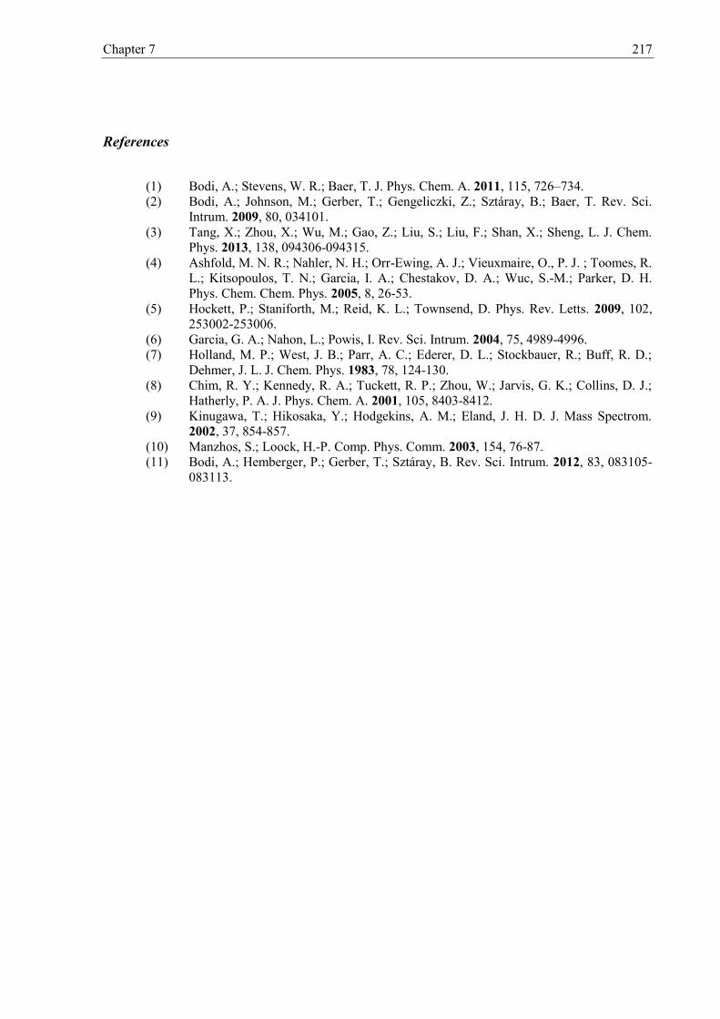
Chapter 7 217

References

(1) Bodi, A.; Stevens, W. R.; Baer, T. J. Phys. Chem. A. 2011, 115, 726–734. (2) Bodi, A.; Johnson, M.; Gerber, T.; Gengeliczki, Z.; Sztáray, B.; Baer, T. Rev. Sci.

Intrum. 2009, 80, 034101. (3) Tang, X.; Zhou, X.; Wu, M.; Gao, Z.; Liu, S.; Liu, F.; Shan, X.; Sheng, L. J. Chem.

Phys. 2013, 138, 094306-094315. (4) Ashfold, M. N. R.; Nahler, N. H.; Orr-Ewing, A. J.; Vieuxmaire, O., P. J. ; Toomes, R.

L.; Kitsopoulos, T. N.; Garcia, I. A.; Chestakov, D. A.; Wuc, S.-M.; Parker, D. H. Phys. Chem. Chem. Phys. 2005, 8, 26-53.

(5) Hockett, P.; Staniforth, M.; Reid, K. L.; Townsend, D. Phys. Rev. Letts. 2009, 102, 253002-253006.

(6) Garcia, G. A.; Nahon, L.; Powis, I. Rev. Sci. Intrum. 2004, 75, 4989-4996. (7) Holland, M. P.; West, J. B.; Parr, A. C.; Ederer, D. L.; Stockbauer, R.; Buff, R. D.;

Dehmer, J. L. J. Chem. Phys. 1983, 78, 124-130. (8) Chim, R. Y.; Kennedy, R. A.; Tuckett, R. P.; Zhou, W.; Jarvis, G. K.; Collins, D. J.;

Hatherly, P. A. J. Phys. Chem. A. 2001, 105, 8403-8412. (9) Kinugawa, T.; Hikosaka, Y.; Hodgekins, A. M.; Eland, J. H. D. J. Mass Spectrom.

2002, 37, 854-857. (10) Manzhos, S.; Loock, H.-P. Comp. Phys. Comm. 2003, 154, 76-87. (11) Bodi, A.; Hemberger, P.; Gerber, T.; Sztáray, B. Rev. Sci. Intrum. 2012, 83, 083105-

083113.

Appendix I 218

Appendix I:

Chapter 4

Tables of 0 K total energies including the zero point energies which were calculated using a

variety of ab initio techniques and the results of varying the weighting of different input

parameters into the network, and used in Chapter 4, are presented below.

Appendix I 219

Table 1.1. Total 0 K energies including the zero point energy calculated with G3B3 and W1 methods, with total 0 K energies calculated by Csontos. Species highlighted in yellow are the values fitted in this work to derive new enthalpies of formation.

Species G3B3 (0K) H W1 (0K) H Csontos neutrals ∆fHo0K (H)

CHCl3 -1418.833349 -1423.181789 -1423.643557 CH2Cl2 -959.374641 -962.281806 -962.591305 CH3Cl -499.915194 -501.379808 -501.537503 CCl4 -1878.288639 -1884.07676 -1884.690439 CH2Cl+ -498.938772 -500.401326

CHCl2+ -958.419567 -961.324125

CCl3+ -1417.889685 -1422.235445

CH3+ -39.431362 -39.452772

CH3F -139.652064 -139.800335 -139.820583 CH2F2 -238.866356 -239.142222 -239.175648 CHF3 -338.092025 -338.495796 -338.542544 CF4 -437.314451 -437.846106 -437.907502 CH4 -40.45827 -40.479069

CH2F+ -138.659846 -138.809009

CHF2

+ -237.88441 -238.161657

CF3

+ -337.088561 -337.493773

CF3Cl -797.552468 -799.39851 -799.597683 CF2Cl2 -1157.79383 -1160.953894 -1161.291212 CFCl3 -1518.038981 -1522.513079 -1522.988716 CHClF2 -698.333114 -700.052131 -700.23742 CCl2F+ -1057.624228 -1060.656081

CClF2+ -697.358671 -699.076885

CBrClF2 -3271.296242

Appendix I 220

Table 1.2. Enthalpies of formation from a relaxed fit with no error minimization and the weighted (with values given in text) relaxed fit where all values except anchor values are included in the fit. Values highlighted in yellow are the final fit parameters, those highlighted in blue are the fixed anchor values. Species no weight relaxed fit ∆fHo

0K kJ mol-1 fit

weighted relaxed fit ∆fHo0K kJ mol-1 fit

CHCl3 anchor -98.40

anchor -98.40

CH2Cl2 -87.93

-87.89 CH3Cl -75.01

-75.62

CCl4 -94.77

-94.82 CH2Cl+ 962.15

960.79

CHCl2+ 893.82

890.32

CCl3+ 857.21

850.06

CH3+ anchor 1099.35

anchor 1099.35

CH3F -226.87

-227.44 CH2F2 -441.45

-442.34

CHF3 -687.16

-687.75 CF4 anchor -927.80

anchor -927.80

CH4 -66.56

-66.56 CH2F+ 846.14

845.38

CHF2+ 602.57

601.72

CF3+ anchor 413.40

anchor 413.40

CF3Cl -704.88

-704.68 CF2Cl2 -490.75

-490.36

CFCl3 -287.06

-286.47 CHClF2 -476.09

-475.70

CCl2F+ 706.14

701.37 CClF2

+ 554.63

552.24 CBrClF2 -444.14

-446.52

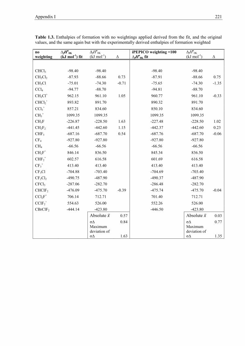
Appendix I 221

Table 1.3. Enthalpies of formation with no weightings applied derived from the fit, and the original values, and the same again but with the experimentally derived enthalpies of formation weighted

no weighting

∆fHo0K

(kJ mol-1) fit ∆fHo

0K (kJ mol-1) Δ

iPEPICO weighting =100 ∆fHo

0K fit ∆fHo

0K (kJ mol-1) Δ

CHCl3 -98.40 -98.40

-98.40 -98.40

CH2Cl2 -87.93 -88.66 0.73 -87.91 -88.66 0.75 CH3Cl -75.01 -74.30 -0.71 -75.65 -74.30 -1.35 CCl4 -94.77 -88.70

-94.81 -88.70

CH2Cl+ 962.15 961.10 1.05 960.77 961.10 -0.33 CHCl2

+ 893.82 891.70

890.32 891.70 CCl3

+ 857.21 834.60

850.10 834.60 CH3

+ 1099.35 1099.35

1099.35 1099.35 CH3F -226.87 -228.50 1.63 -227.48 -228.50 1.02

CH2F2 -441.45 -442.60 1.15 -442.37 -442.60 0.23 CHF3 -687.16 -687.70 0.54 -687.76 -687.70 -0.06 CF4 -927.80 -927.80

-927.80 -927.80

CH4 -66.56 -66.56

-66.56 -66.56 CH2F+ 846.14 836.50

845.34 836.50

CHF2+ 602.57 616.58

601.69 616.58

CF3+ 413.40 413.40

413.40 413.40

CF3Cl -704.88 -703.40

-704.69 -703.40 CF2Cl2 -490.75 -487.90

-490.37 -487.90

CFCl3 -287.06 -282.70

-286.48 -282.70 CHClF2 -476.09 -475.70 -0.39 -475.74 -475.70 -0.04

CCl2F+ 706.14 712.71

701.40 712.71 CClF2

+ 554.63 526.00

552.26 526.00 CBrClF2 -444.14 -423.80

-446.50 -423.80

Absolute 0.57 Absolute 0.03

σΔ 0.84 σΔ 0.77

Maximum deviation of σΔ 1.63

Maximum deviation of σΔ 1.35

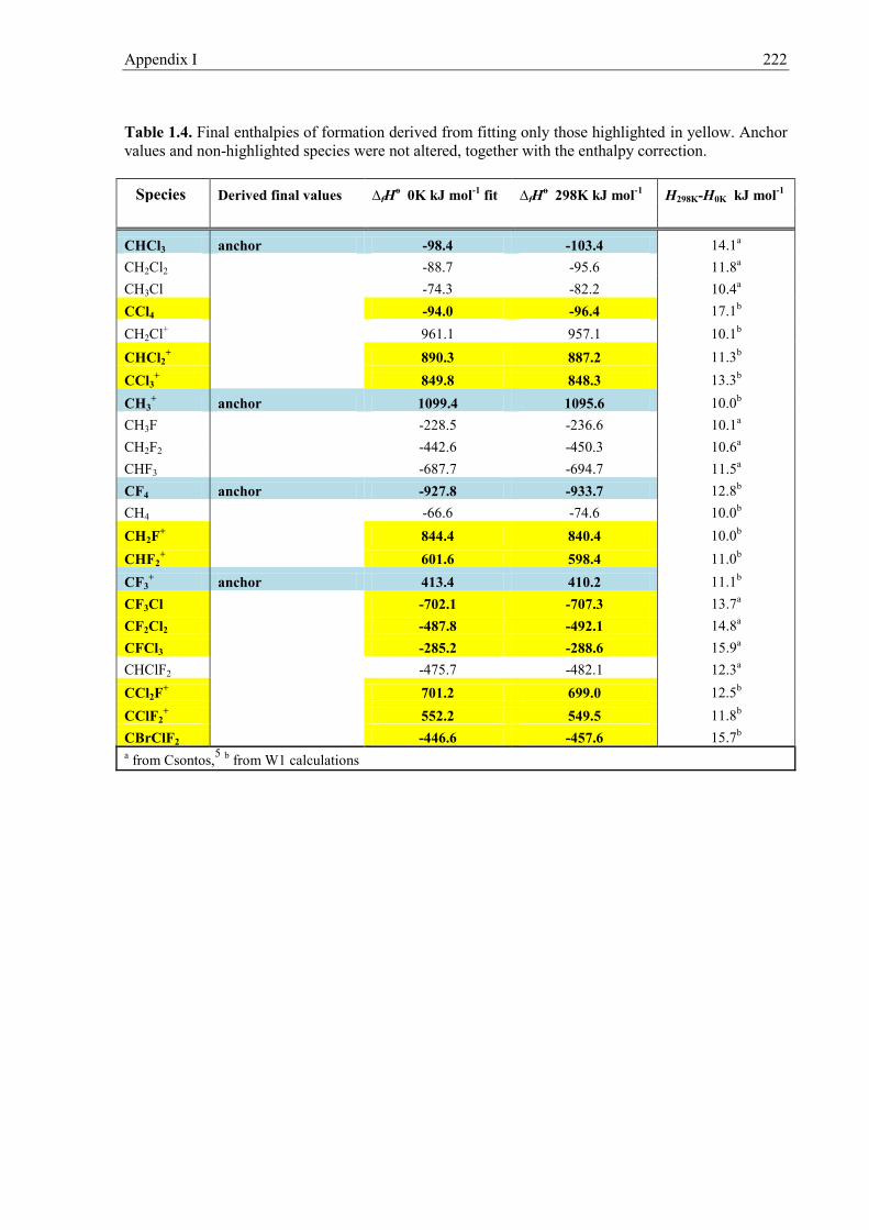
Appendix I 222

Table 1.4. Final enthalpies of formation derived from fitting only those highlighted in yellow. Anchor values and non-highlighted species were not altered, together with the enthalpy correction. Species Derived final values ∆fHo 0K kJ mol-1 fit ∆fHo 298K kJ mol-1 H298K-H0K kJ mol-1

CHCl3 anchor -98.4 -103.4 14.1a

CH2Cl2 -88.7 -95.6 11.8a

CH3Cl -74.3 -82.2 10.4a

CCl4 -94.0 -96.4 17.1b

CH2Cl+ 961.1 957.1 10.1b

CHCl2+ 890.3 887.2 11.3b

CCl3+ 849.8 848.3 13.3b

CH3+ anchor 1099.4 1095.6 10.0b

CH3F -228.5 -236.6 10.1a

CH2F2 -442.6 -450.3 10.6a

CHF3 -687.7 -694.7 11.5a

CF4 anchor -927.8 -933.7 12.8b

CH4 -66.6 -74.6 10.0b

CH2F+ 844.4 840.4 10.0b

CHF2+ 601.6 598.4 11.0b

CF3+ anchor 413.4 410.2 11.1b

CF3Cl -702.1 -707.3 13.7a

CF2Cl2 -487.8 -492.1 14.8a

CFCl3 -285.2 -288.6 15.9a

CHClF2 -475.7 -482.1 12.3a

CCl2F+ 701.2 699.0 12.5b

CClF2+ 552.2 549.5 11.8b

CBrClF2 -446.6 -457.6 15.7b

a from Csontos,5 b from W1 calculations

Appendix I 223

Table 1.5. Enthalpies of formation derived with the experimental data at different weightings. The final values used with a weighting of 100 for the experimental onsets are highlighted in yellow .

∆fHo0K (kJ mol–1)

iPEPICO weighting = 1.0 10.0 100.0 1000.0 10000.0 variance

CHCl3 -98.4 -98.4 -98.4 -98.4 -98.4 0.0 CH2Cl2 -87.9 -88.1 -87.9 -88.1 -88.1 0.2 CH3Cl -75.0 -75.5 -75.6 -75.9 -75.9 0.9 CCl4 -94.8 -94.6 -94.8 -94.8 -94.8 0.2 CH2Cl+ 962.2 960.8 960.8 960.5 960.5 1.6 CHCl2

+ 893.8 890.3 890.3 890.3 890.3 3.5 CCl3

+ 857.2 850.0 850.1 853.4 853.4 7.2 CH3

+ 1099.4 1099.4 1099.4 1099.4 1099.4 0.0 CH3F -226.9 -227.4 -227.5 -227.3 -227.3 0.6 CH2F2 -441.5 -442.2 -442.4 -442.2 -442.2 0.9 CHF3 -687.2 -687.7 -687.8 -687.7 -687.7 0.6 CF4 -927.8 -927.8 -927.8 -927.8 -927.8 0.0 CH4 -66.6 -66.6 -66.6 -66.6 -66.6 0.0 CH2F+ 846.1 845.5 845.3 845.5 845.5 0.8 CHF2

+ 602.6 601.8 601.7 601.8 601.8 0.9 CF3

+ 413.4 413.4 413.4 413.4 413.4 0.0 CClF3 -704.9 -704.8 -704.7 -704.6 -704.6 0.3 CF2Cl2 -490.8 -490.5 -490.4 -490.3 -490.3 0.5 CFCl3 -287.1 -286.7 -286.5 -286.5 -286.5 0.6 CHClF2 -476.1 -475.8 -475.7 -475.6 -475.6 0.5 CCl2F+ 706.1 701.4 701.4 703.5 703.5 4.8 CClF2

+ 554.6 552.2 552.3 553.3 553.2 2.4 CBrClF2 -444.1 -446.5 -446.5 -445.5 -445.5 2.4

Appendix I 224

Table 1.6. Ab initio calculated enthalpies of formation, values from the Csontos study and an example of how the values change, fit, is given in the last column

G3B3 ∆rH

o (0K) Hartrees

CBS-QB3 ∆rHo

(0K) Hartrees

CBS-APNO ∆rH

o (0K) Hartrees

W1 ∆rHo (0K)

Hartrees Csontos ∆rH

o neutrals Hartrees

CHCl3 -1418.833349 -1417.870203

-1423.181789 -1423.643557

CH2Cl2 -959.374641 -958.716555

-962.281806 -962.591305

CH3Cl -499.915194 -499.562049

-501.379808 -501.537503

CCl4 -1878.288639 -1877.02021

-1884.07676 -1884.690439

CH2Cl+ -498.938772 -498.585752

-500.401326

CHCl2+ -958.419567 -957.760866

-961.324125

CCl3+ -1417.889685 -1416.925283

-1422.235445

CH3+ -39.431362 -39.384653 -39.441329 -39.452772

Cl2 -920.073632 -919.46121

-922.95813 -923.262458

F2 -199.428914 -199.512588 -199.512588 -199.681939 -199.711184

Br2 -5147.110006

Cl2 bond energy (H) 0.091106469

F2 bond energy (H) 0.058884031

Br2 bond energy (H) 0.072806714

H atom -0.501087 -0.499946 -0.499946 -0.499994

Appendix I 225

G3B3 (0K) Hartrees

CBS-QB3 (0K) Hartrees

CBS-APNO (0K) Hartrees

W1 (0K) Hartrees Csontos neutrals

CH3F -139.652064

-139.704352 -139.800335 -139.820583

CH2F2 -238.866356

-238.960936 -239.142222 -239.175648

CHF3 -338.092025

-338.229582 -338.495796 -338.542544

CF4 -437.314451

-437.495364 -437.846106 -437.907502

CH4 -40.45827 -40.41 -40.468934 -40.479069

CH2F+ -138.659846

-138.713079 -138.809009

CHF2+ -237.88441

-237.980973 -238.161657

CF3+ -337.088561

-337.22847 -337.493773

CClF3 -797.552468 -797.07839

-799.39851 -799.597683

CF2Cl2 -1157.79383

-1160.953894 -1161.291212

CFCl3 -1518.038981 -1517.035241

-1522.513079 -1522.988716

CHClF2 -698.333114

-700.052131 -700.23742

CHCl2F -1058.580311

-1061.614077 -1061.937489

CHClF+ -598.150912 -597.757429

-599.741333

CCl2F + -1057.624228 -1056.925016

-1060.656081

CClF2+ -697.358671 -696.924563

-699.076885

Appendix I 226

G3B3 (0K) Hartrees

CBS-QB3 (0K) Hartrees

CBS-APNO (0K) Hartrees

W1 (0K) Hartrees Csontos neutrals

CBrClF2 -3271.296242

CBr2F2 -5384.798755

CBr4 -10332.30704

CF3Br -2911.054215

CH3Br -2613.42163

Appendix II 227

Appendix II:

Chapter 4 and 5

Input data for modelling the breakdown curves in Chapter 4, calculated with B3LYP/6-311++G** basis set and level of theory using Gaussian 03.

CH3Cl

Neutral frequencies / cm–1 710, 1025, 1025, 1377, 1483, 1483, 3072, 3167, 3167 Neutral rotational constants / Hz 157502390000, 13096080000, 13096020000

Ion frequencies / cm–1 173, 634, 825, 1158, 1226, 1414, 2778, 3061 Transition state 1 frequencies / cm–1 485, 499, 1288, 1404, 1532, 3062, 3261, 3268

CH2Cl2

Neutral frequencies / cm–1 283, 704, 727, 914, 1196, 1321, 1489, 3144, 3223 Neutral rotational constants / Hz

32180670000, 3194240000, 2961290000

Ion frequencies / cm–1 262, 600, 743, 963, 1110, 1274, 1470, 3155, 3265 Transition state 1 frequencies / cm–1

243, 702, 892, 1054, 1134, 1452, 3125, 3266

CHCl3


3197290000, 3197290000, 1657110000


146, 287, 350, 739, 931, 976, 1291, 3193

Appendix II 228

CH3F


156698870000, 25583990000, 25583990000


194, 252, 1214, 1232, 1410, 1552, 3049, 3222

CH2F2


490631000000, 104471300000, 91377600000


154, 178, 660, 1019, 1302, 1347, 1604, 3151

CBrClF2


3813310000, 1649540000, 1443260000


162, 217, 402, 472, 549, 729, 1233, 1372

CHClF2


10190040000, 4752230000, 3446910000


54, 116, 662, 1012, 1304, 1352, 1602, 3155

Appendix II 229

Input data for modelling the breakdown curves in Chapter 5, calculated with B3LYP/6-311+G** basis set and level of theory using Gaussian 03.

Monofluorethene

Neutral frequencies / cm–1

484, 733, 871, 952, 977, 1191, 1350, 1441, 1742, 3192, 3216, 3285

Neutral rotational constants / Hz

65687710000, 10529410000, 9074770000

Ion frequencies / cm–1 399, 486, 873, 989, 1013, 1253, 1333, 1469, 1587, 3173, 3216, 3293 Transition state 1 frequencies / cm–1

341, 540, 718, 744, 777, 846, 1144, 1600, 1671, 3206, 3260

Transition state 2 frequencies / cm–1

148, 246, 363, 389, 808, 824, 1069, 1279, 2103, 3031, 3141

Transition state 1 = HF loss, transition state 2 = H loss

1,1-difluorethene


430, 495, 572, 725, 868, 919, 953, 1260, 1451, 1763, 3194, 3293


10245430000, 10121060000, 5091430000

Ion frequencies / cm–1 373, 417, 582, 627, 922, 958, 1005, 1428, 1515, 1578, 3140, 3268


87, 433, 496, 557, 573, 739, 1099, 1208, 1327, 2117, 3197


408, 465, 610, 918, 959, 1081, 1200, 1444, 1530, 3122, 3260

Transition state 1 = HF loss, transition state 2 = F loss

Trifluorethene


226, 306, 480, 556, 620, 775, 946, 1191, 1298, 1395, 1851, 3270


10517160000, 3832250000, 2808780000

Ion frequencies / cm–1 221, 234, 486, 567, 639, 798, 959, 1287, 1415, 1573, 1667, 3234 Transition state 1 frequencies / cm–1

35, 74, 112, 197, 621, 723, 1234, 1281, 1468, 1506, 3213


35, 74, 112, 197, 621, 723, 1234, 1281, 1468, 1506, 3213


15, 54, 75, 123, 146, 649, 1094, 1256, 1282, 1497, 2787

Transition state 1 = CF loss, transition state 2 = CHF loss, transition state 3 = CF2 loss

Appendix II 230

Tetrafluorethene


193, 200, 391, 415, 480, 544, 545, 798, 1201, 1361, 1367, 1928


5411200000, 3225030000, 2020710000

Ion frequencies / cm–1 137, 208, 400, 426, 530, 548, 591, 834, 1296, 1568, 1569, 1725 Transition state 1 frequencies Regime 1 / cm–1

19, 43, 46, 110, 472, 540, 541, 912, 1473, 1513, 1514

Transition state 2 frequencies Regime 1 / cm–1

30, 65, 72, 152, 110, 472, 540, 541, 912, 1473, 1513, 1514

Transition state 3 frequencies regime 1 / cm–1

19, 45, 50, 98, 116, 607, 663, 1149, 1321, 1388, 1395

Neutral frequencies regime 2 / cm–1

193, 200, 391, 415, 480, 544, 545, 798, 1201, 1361, 1367, 1928

Neutral rotational constants regime 2 / Hz

5411200000, 3225030000, 2020710000

Ion frequencies regime 2 / cm–1

137, 208, 400, 426, 530, 548, 591, 834, 1296, 1568, 1569, 1725


25, 40, 60, 200, 220, 400, 426, 530, 548, 591, 834, 1296, 1568, 1569, 1725


25, 40, 60, 200, 220, 400, 426, 530, 548, 591, 834, 1296, 1568, 1569, 1725

Regime 1; Transition state 1 = CF loss, transition state 2 = CF3 loss, transition state 3 = CF2 loss Regime 2: Transition state 1= F loss, transition state 2 = CF2 + F loss

Appendix II 231

Figure 2.1. Screenshots of breakdown curve modelling program as described in Chapter 3.

Appendix III 232

Appendix III:

Threshold photoelectron spectra of halogenated

methanes recorded with the iPEPICO apparatus

at the VUV beamline at the Swiss Light Source

Acknowledgement is given to Dr Andras Bodi, Dr Melanie Johnson, Nicola Rogers, Dr

Matthew Simpson, and Prof. Richard Tuckett for assistance with data collection. All spectra

are normalized to sample pressure and photon flux.

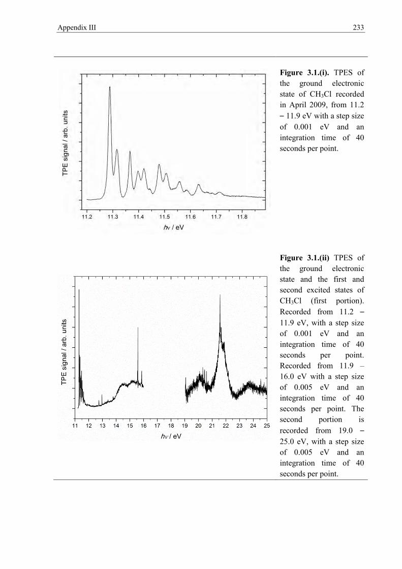
Appendix III 233

Figure 3.1.(i). TPES of the ground electronic state of CH3Cl recorded in April 2009, from 11.2 – 11.9 eV with a step size of 0.001 eV and an integration time of 40 seconds per point.

Figure 3.1.(ii) TPES of the ground electronic state and the first and second excited states of CH3Cl (first portion). Recorded from 11.2 – 11.9 eV, with a step size of 0.001 eV and an integration time of 40 seconds per point. Recorded from 11.9 – 16.0 eV with a step size of 0.005 eV and an integration time of 40 seconds per point. The second portion is recorded from 19.0 – 25.0 eV, with a step size of 0.005 eV and an integration time of 40 seconds per point.

Appendix III 234

Figure 3.2.(i). TPES of the ground and first electronic state of CH2Cl2 recorded in April 2009, from 11.05 – 11.30 eV with a step size of 0.003 eV and an integration time of 40 seconds per point.

Figure 3.2.(ii) TPES of the ground and first electronic state and the first and second excited states of CH2Cl2 Recorded from 11.05 – 11.30 eV, with a step size of 0.003 eV and an integration time of 40 seconds per point. Recorded from 11.30 – 15.7 eV with a step size of 0.003 eV and an integration time of 40 seconds per point.

Appendix III 235

Figure 3.3.(i). TPES of the ground, first and second excited electronic state of CHCl3 recorded in March 2009, from 11.00 – 15.71 eV with a step size of 0.003 eV and an integration time of 26 s per point. Inset shows as more detailed spectrum from 12.60 – 13.20 with a step size of 0.001 eV and an integration time of 44 s.

Figure 3.3.(ii) TPES of the ground, first second, third and fourth excited electronic state and the first and second excited states of CCl4 Recorded from 11.00 – 14.00 eV, with a step size of 0.003 eV and an integration time of 40 s per point. Recorded from 14.0 – 21 eV with a step size of 0.02 eV and an integration time of 60 s per point. Inset, recorded 13.10 – 13.80 eV, 40 s integration time, 0.002 step size.

Appendix III 236

Figure 3.4.(i). TPES of the ground electronic state of CH2F2 recorded in August 2010, from 12.65 – 13.85 eV, with an integration time of 90 s and a step size of 0.002 eV

Figure 3.4.(ii). TPES of the ground and first six excited electronic states of CH2F2 recorded in August 2010. 12.65 – 13.85 eV, with an integration time of 30 s and a step size of 0.002 eV. 14.60 – 16.40 eV, with an integration time of 30 s and a step size of 0.002 eV, 16.40 – 18.00 eV, with an integration time of 30 s and a step size of 0.006 eV, 18.00 – 19.80 eV, with an integration time of 30 s and a step size of 0.002 eV

Appendix III 237

Figure 3.5. TPES of the ground and first six excited electronic states of CH3F recorded in August 2010. 12.48 – 13.60 eV with a step size of 0.001 eV, integration time 35. 13.60 –

13.93 eV with a step size of 0.002 eV and integration tome of 35 s.

Appendix IV 238

Appendix IV:

Ion images

Raw ion images of CF3+, SF5

+ and CCl4+ as captured by the Roentdek DLD40 detector, using

a thermal gas source. Contamination in the images by background signal originating from

O2+ and N2

+ account for the strong central spot in each image. The total kinetic energy

release is plotted for CF3+, and CCl4

+ across the energy ranges of the first photoelectron

bands. The raw images were reconstructed with the onion peeling algorithm. The radius of

the image is proportional to the kinetic energy release. Argon was used to calibrate the

images as once the Ar+ formed, and excess energy is carried away by the electron, so the

radius of the Argon image is equal to to 3/2 kBT or 0.038 eV. All ions were extracted with

fields of 80 V cm–1.

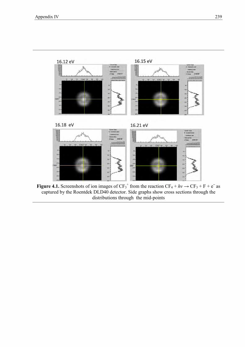
Appendix IV 239

Figure 4.1. Screenshots of ion images of CF3

+ from the reaction CF4 + hv → CF3 + F + e– as captured by the Roentdek DLD40 detector. Side graphs show cross sections through the

distributions through the mid-points

Appendix IV 240

Figure 4.2 Kinetic energy release of CF3

+ energy release of CF3+ from the reaction CF4 + hv

→ CF3 + F + e– . The 2-dimensional image was reconstructed using with the onion peeling algorithm, see Chapter 7. The radius of the image is proportional to the kinetic energy release. The CF3

+ images were calibrated using the radius of the Argon image at 15.71 eV which is equal to 3/2 kBT or 0.038 eV.

Appendix IV 241

Figure 4.3. Screenshots of ion images of CCl4

+ from the reaction CCl4 + hv → CCl3+ + Cl +

e– as captured by the Roentdek DLD40 detector. Side graphs show cross sections through the distributions through the mid-points

Appendix IV 242

Figure 4.4. Kinetic energy release of CCl3

+ from the reaction CCl4 + hv → CCl3+ + Cl + e–.

The 2-dimensional image was reconstructed using with the onion peeling algorithm, see Chapter 7. The radius of the image is proportional to the kinetic energy release. The CF3

+

images were calibrated using the radius of the Argon image at 15.71 eV which is equal to 3/2 kBT or 0.038 eV.

Appendix IV 243

Figure 4.5. Screenshots of ion images of SF5

+ from the reaction SF6 + hv → SF5 + F + e– as captured by the Roentdek DLD40 detector, showing clear anisotropy, perpendicular to the electric vector of the VUV light. Side graphs show cross sections through the distributions

through the mid-points

Modelling the dissociation dynamics and threshold...

Documents

Transcript of Modelling the dissociation dynamics and threshold...