Math Geosci (2010) 42: 519–534DOI 10.1007/s11004-010-9293-6

S P E C I A L I S S U E

Modelling Syntectonic Sedimentation: Combininga Discrete Element Model of Tectonic Deformationand a Process-based Sedimentary Model in 3D

A. Carmona · R. Clavera-Gispert · O. Gratacós ·S. Hardy

Received: 17 November 2009 / Accepted: 28 May 2010 / Published online: 11 June 2010© International Association for Mathematical Geosciences 2010

Abstract This paper presents a new numerical program able to model syntectonicsedimentation. The new model combines a discrete element model of the tectonicdeformation of a sedimentary cover and a process-based model of sedimentation in asingle framework. The integration of these two methods allows us to include the sim-ulation of both sedimentation and deformation processes in a single and more effec-tive model. The paper describes briefly the antecedents of the program, Simsafadim-Clastic and a discrete element model, in order to introduce the methodology usedto merge both programs to create the new code. To illustrate the operation and ap-plication of the program, analysis of the evolution of syntectonic geometries in anextensional environment and also associated with thrust fault propagation is under-taken. Using the new code, much more complex and realistic depositional structurescan be simulated together with a more complex analysis of the evolution of the de-formation within the sedimentary cover, which is seen to be affected by the presenceof the new syntectonic sediments.

Keywords Process based sedimentary models · Discrete element technique ·Syntectonic sedimentation

A. Carmona (�) · O. Gratacós · S. HardyGEOMODELS Research Institute, and GGAC Grup de Geodinàmica i Anàlisis de Conques, Facultatde Geologia, Universitat de Barcelona, c/Martí i Franquès s/n, 08028 Barcelona, Catalonia, Spaine-mail: anacarmona@ub.edu

R. Clavera-GispertAbteilung Geologie, Facultat für Biologie, cheime und Geowissenschaften, Universität Bayreuth,Bayreuth, Germany

S. HardyIcrea (Institució Catalana de Recerca i Estudis Avançats), Barcelona, Catalonia, Spain

520 Math Geosci (2010) 42: 519–534

1 Introduction

As a result of improvements in computer technology since the 1970s, numericalmodelling has become an essential tool in the analysis of geological processes. Nu-merical modelling may assist the understanding of geometries, architectures, andprocesses difficult to otherwise observe in nature or to understand by simple con-ceptual models. Moreover, it has also become a useful validation tool for othermethods such as 3D reconstruction or analogue modelling. There are many pub-lished numerical models of sedimentation in basins (e.g. Tetzlaff and Harbaugh 1989;Li and Amos 2001). These have treated the simulation of sedimentation from dif-ferent points of view and using different techniques (e.g. Grajeon and Joseph 1999;Hardy and Gawthorpe 1998), and they can provide physical, chemical, and petrologicinformation about different sedimentary bodies. These numerical tools also allowthe prediction of the spatial and temporal distribution of these sedimentary bodiesand their internal architectures. Similarly, there is a wide range of tools, includingkinematic (e.g. Hardy and McClay 1999) and mechanical models (e.g. Allmendinger1998; Johnson and Johnson 2002; Simpson 2006; Strayer and Suppe 2002), able tosimulate deformation at scales from a thin sedimentary cover to full orogenic geome-tries. A variety of numerical techniques have been used to implement these models,ranging from finite elements (e.g. Cardozo et al. 2003) to discrete elements (e.g. Finchet al. 2003, 2004).

Considering the importance of deformation processes on final geometry, as wellas fracture and deformation patterns of sedimentary bodies, it is necessary to con-sider deformation and sedimentary processes at the same time. If this approach isadopted, a more realistic geological model may be obtained. Both processes workingtogether imply more than each working separately because one process is affectedby the other and vice versa (i.e. there is feedback and interaction). From the point ofview of the deformation, the addition of new sediments to a deforming section affectsits evolution. On the other hand, deformation affects previously deposited sedimentsand basin geometries, thus creating a depositional environment that is going to di-rectly affect the deposition of new sediments. Some numerical modelling approachesare able to reproduce both sedimentation and deformation at the same time, treat-ing their interaction in 2D and also 3D. Some are focussed on how the deformationrate is affected by sedimentation and erosion (e.g. Maniatis et al. 2009), while othersjust include sedimentation as an additional phenomenon in the study of crustal rockssubject to specific tectonic boundary conditions (e.g. Gawthorpe and Hardy 2002;Simpson 2009). However, in these papers, transport and sedimentation processes aremodelled either by a simple diffusive equation or treated simply as a refill process,but not as a real process that follows physical rules of transport and sedimentation.

To combine realistic models of deformation and sedimentation is the main aimof the new numerical computer program presented here. A new code has been de-veloped to combine mechanical and sedimentary process-based numerical models.Combining these two approaches allows us to include the simulation of both sedi-mentation and deformation processes in a single and more realistic model. This newtool results from the merging of two previous published works: Simsafadim-Clastic(Bitzer and Salas 2002; Gratacós 2004; Gratacós et al. 2009a) and a discrete element

Math Geosci (2010) 42: 519–534 521

model or DEM (Finch et al. 2003, 2004; Hardy and Finch 2005, 2006, 2007; Hardyet al. 2009). The former simulates sub-aquatic clastic transport and sedimentation inthree dimensions, including processes of interaction, production, and sedimentationof carbonates; moreover, it is also a powerful tool for the 3D prediction of strati-graphic structures and facies distribution modelling in sedimentary basins. The latterdeals with the simulation of the deformation in sedimentary rocks in 2D and 3D. Thisdeformation is a consequence of interaction of many individual elements accordingto mechanical rules. The main goal of merging these two methods is to develop a newtool that will be able to offer a more complex and realistic study of the evolution ofthe structures and deformation in sedimentary materials produced by faults and folds.Deformation is based on mechanical rules and is therefore influenced by the presenceof syntectonic sediments. In addition, the tectonic processes change the topographicsurface, which influences fluid flow, transport, and, consequently, sedimentation inthe process-based sedimentary model. Finally, analysis of the evolution of deforma-tion within these new syntectonic materials can also be performed. The understandingof the development and characteristics of these syntectonic architectures is importantin many areas of structural geology, such as hydrocarbon prospecting and evaluatingthe stratigraphic architectures in sedimentary basins, among others.

2 Combining Process-based Sedimentary Models and Discrete ElementModelling

2.1 Background

For a better and easier understanding of how the new code works, it is essential to givea short overview of the procedure and methodology of its component parts. We nowsummarize how Simsafadim-Clastic and the discrete element model work. For moredetailed information on both codes, the reader is referred to more detailed descrip-tions in Gratacós (2004), Gratacós et al. (2009a, 2009b) for the Simsafadim-Clasticprogram; see Finch et al. (2004) and Hardy and Finch (2005) for the DEM program.

2.1.1 Simsafadim-Clastic

Simsafadim-Clastic program is a 3D process-based numerical forward model, whichsimulates clastic transport and sedimentation including carbonate production, trans-port, and sedimentation. Initial basin topography is discretized using triangular finiteelements. These elements will be the basis to develop and solve the differential equa-tion that manages the fluid flow and transport processes. The nodes of these trianglesare also used to solve the remaining equations that describe sedimentation and car-bonate production. Total simulation time is discretized according to the Courant crite-rion, which gives interval time steps to ensure the stability of the differential equationsolutions (Gratacós 2004). The fluid flow system is a 2D potential model (Bitzer andSalas 2002) in a transitional pattern. It assumes a laminar, non-viscid, and irrotationalfluid, without short-time processes. The fluid flow value in each node depends on thewater depth, but it is considered constant along the water column. The equation is

522 Math Geosci (2010) 42: 519–534

solved using the finite element method (Kinzelbach 1986). The transport model as-sumes that the sediment is transported in suspension mainly by advection processesas a result of the fluid flow velocity. It also considers dispersion and diffusion termsas a result of shorter transport processes such as organic activity or wave action. Thesediment is uniformly distributed in the water column in order to simulate a turbulenttransport process. The transport equation is also solved by the finite element methodfor each clastic sediment type (Kinzelbach 1986). The sedimentation model assumesthat a particle is susceptible to settling when the fluid flow linear velocity is lowerthan a critical settling velocity. This critical settling velocity is defined for each sed-iment type according to its density and its grain size. The final settling velocity of aparticle is modified according to a linear dependence between the flow linear velocityand its theoretical critical settling velocity. Despite the fact that Simsafadim-Clasticcan efficiently model the distribution of facies and the depositional architectures in asedimentary basin, the program has some limitations that can affect the final result.The main limitation is the static basement consideration as no tectonic movementsare considered, although the program considers isostacy as well as subsidence due tothe weight of the new materials.

2.1.2 Discrete Element Modelling (DEM)

The discrete element technique is used to model and investigate, in 2D and 3D, thepropagation and evolution of deformations in sedimentary cover caused by tectonicmovements that affects the rigid boundary of the model, e.g. detachment folding(Hardy and Finch 2006), thrust/extensional fault-propagation folds (Finch et al. 2003,2004; Hardy and Finch 2005), doubly vergent thrust wedges (Hardy et al. 2009) andevolution of calderas (Hardy 2008). The model approach is a variant of the “LatticeSolid Model” (Mora and Place 1993, 1994). A detailed description of the LSM isgiven by the cited articles. An outline of the model approach and its implementa-tion is given here (for a full description, also see Finch et al. 2004; Hardy and Finch2005). An assemblage of spherical elements of different radii is used to model therock mass; this allows a random position of the elements avoid any isotropy or anylikelihood for preferred planes of weakness (Hardy and Finch 2006). The evolution ofthe system is realized through the interaction and behaviour of these elements. Thesediscrete elements interact in pairs through a repulsive–attractive force as if they areconnected by breakable elastic springs. A breaking separation is defined, a particleis bonded until the separation between them exceeds this lower limit, and after thatthe bond is irreparably broken. Nevertheless, the repulsive force can act again be-tween them if the particle pair goes back to a compressive contact. To calculate thetotal elastic force applied on a particle is only necessary to do the sum of the forceson each bond that link the particle to its neighbours. The body is elastic–plastic andcan consider friction. But the precise mechanics of the assemblage are not discussedhere. The importance is the transfer of the resultant deformation to the sedimentarymodel. The gravitational force, acting in each element, is also added. In addition,a viscous damping term is included. This viscous term is proportional to the parti-cle velocity and it is considered in order to make the model less dynamic and morequasi-static, which is more suitable for modelling the development of tectonic struc-tures over long time scales. This assemblage is confined into a bounding box. The

Math Geosci (2010) 42: 519–534 523

base of the box is supposed to be the basement and is considered to be rigid and un-deformable, only affected by the small displacements with which the deformation issimulated. These displacements are performed to the bounding box in each time stepaccording to the boundary conditions chosen: a normal fault, strike-slip, a detachmentfold, etc. The time step is chosen to ensure numerical precision and stability (Moraand Place 1994). At each discrete time step, particles proceed to their new positionby integrating their equation of motion using Newtonian physics and velocity VerlatScheme (Allen and Tidsley 1987). Some 2D configurations of this model allow us toadd syntectonic materials during the evolution of the model, but this is just a refillof the created accommodation space, not a real process of sedimentation. Not con-sidering sedimentation process during the evolution of the model is the current mainlimitation of the discrete element model.

2.2 Merging

Taking into account the limitations of Simsafadim-Clastic and DEM, merging pro-vides us a new tool for geological modelling that addresses the main limitations ofboth programs, complementing each other. The new tool can predict and analyseother different syntectonic depositional architectures with more complex geologi-cal scenarios. It also allows a more realistic study of the evolution of deformationproduced by faults and folds since the contribution of new sediments to the sys-tem is considered. Sediments come from a source and they undergo transport andsettle, which are also a function of the new relief that is constructed. An appro-priate approach to combing both codes would be to create a link between the twomodels that allows us to run them separately without mixing up the two methods.This link is created using the spheres located on the assemblage surface that de-fine the initial topography of the basin used by the Simsafadim-Clastic program.The idea is that this initial basin topography, discretized into a triangular finiteelement mesh, will adapt to the movement of the spheres on the DEM surface.To do this, the mesh is established over this assemblage surface. The z positionof each node is given by the average position of the four spheres of the assem-blage surface located closest to the x–y node position (Fig. 1). To choose thetime step, we checked the requirements of the discretization time for convergenceand stability of the mathematical methods used in each program (Gratacós 2004;Hardy and Finch 2006). The smallest �t is selected in order to ensure proper resultsfor both programs. The two programs are thus run separately but concurrently, andfor each time step �t the interaction between them is calculated and the z valuesof the nodes are updated. This value is determined by the new position of the ballsthat make up the surface at the current time step, plus the sediment that Simsafadim-Clastic had added to each node (which is taken into account by the Simsafadim-Clastic code). This implies that the changes in the topography of the basin are nowcontrolled by two factors: tectonic movements and sedimentation. When the amountof sediment deposited in the model is higher than a critical value (this means having anumber of nodes with an amount of sediment equal to or bigger than the diameter of asphere), a transfer from Simsafadim-Clastic to the discrete element model takes place.In this transfer, the space taken up by the new sediment is refilled with new discrete

524 Math Geosci (2010) 42: 519–534

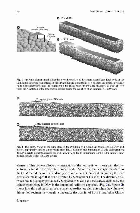
Fig. 1 (a) Finite element mesh allocation over the surface of the sphere assemblage. Each node of theelement looks for the four spheres of the surface that are closest to its x–y position and it takes average z

value of the spheres position. (b) Adaptation of the initial basin surface at the movement of DEM at t = 0years. (c) Adaptation of the topographic surface during the evolution of an example (t = 210 years)

Fig. 2 Two lateral views of the same stage in the evolution of a model: (a) position of the DEM andthe real topography surface which results from DEM evolution plus Simsafadim-Clastic sedimentation;(b) new discrete elements added to the DEM assemblage due to Simsafadim-Clastic sedimentation. Nowthe real surface is also the DEM surface

elements. This process allows the interaction of the new sediment along with the pre-tectonic material in the discrete element model. Moreover, the new spheres added tothe DEM record the most abundant type of sediment at their location (among the fourclastic sediment types that can be treated by Simsafadim-Clastic). The difference be-tween real topography provided by Simsafadim-Clastic and the surface defined by thesphere assemblage in DEM is the amount of sediment deposited (Fig. 2a). Figure 2bshows how this sediment has been converted to discrete elements when the volume ofthis settled sediment is enough to undertake the transfer of from Simsafadim-Clastic

Math Geosci (2010) 42: 519–534 525

to DEM. This interchange allows us to study the propagation of deformation in thenew materials, as well as how these new sediments influence the propagation of de-formation in the pre-existing cover.

3 Examples

In order to illustrate/check the potential of the new program, two simple examplesare presented. The first one considers syntectonic sedimentation associated with anextensional fault in order to analyse the evolution and distribution of sedimentationas a result of the tectonic movement, as well as the obtained syntectonic sedimentaryarchitecture. The second example considering syntectonic sedimentation in a thrustfault propagation environment not only deals with the structure, but also with defor-mation and the way in which the introduction of new sediments affect its evolution.

3.1 Initial Configuration of the Model

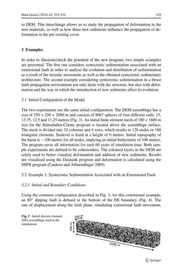
The two experiments use the same initial configuration. The DEM assemblage has asize of 250 × 250 × 2000 m and consists of 8067 spheres of four different radii: 15,13.75, 12.5 and 11.25 metres (Fig. 3). An initial finite element mesh of 180×1800 msize for the Simsafadim-Clastic program is located above the assemblage surface.The mesh is divided into 32 columns and 4 rows, which results in 128 nodes or 186triangular elements. Sealevel is fixed at a height of 0 metres. Initial topography ofthe basin is −100 metres for all nodes, implying an initial bathymetry of 100 metres.The program saves all information for each 60 years of simulation time. Both sam-ple experiments are defined to be cohesionless. The coloured layers in the DEM aresolely used to better visualize deformation and addition of new sediments. Resultsare visualized using the Datatank program and deformation is calculated using theSSPX program (Cardozo and Allmendinger 2009).

3.2 Example 1: Syntectonic Sedimentation Associated with an Extensional Fault

3.2.1 Initial and Boundary Conditions

Using the common configuration described in Fig. 3, for this extensional example,an 80◦ dipping fault is defined in the bottom of the DE boundary (Fig. 4). Therate of displacement along the fault plane, simulating extensional fault movement,

Fig. 3 Initial discrete element(DE) assemblage used in thesimulations

526 Math Geosci (2010) 42: 519–534

Fig. 4 Bounding box of the DE assemblage with an 80◦ dipping fault used in the first example. The arrowshows the direction of relative movement of the hangingwall area (subsidence region) with respect to thefootwall area

Table 1 Sedimentationparameters used for the firstsimulation considering anextensional fault

Clastic 1 Clastic 2 Clastic 3

(fine) (medium) (coarse)

Critical velocity fordeposition (m s−1)

2.5 4.0 5.5

Settle rate(m day−1)

0.003 0.004 0.008

is 0.06 m/year with a total displacement of 96 m in dip direction during the total sim-ulated time (1440 years). Three different clastic sediment types are simulated in themodel. They are characterized through their critical velocity for deposition and rateof settling as summarized in Table 1. These values are higher for coarse materialsand lower for finer ones. Inflow sediment rates are different for the different materialtypes: they are smaller for coarser sediments than for finer ones. The inflow sedimentnodes and rates are defined at a boundary node, as can be observed in Fig. 5. Thefluid flow boundary conditions for the finite element mesh reproduce uniform fluidmovement from the left to the right with initial velocities that allow sedimentation ofthe three different sediment types from the start of the experiment.

3.2.2 Simulation Results

Simulation results are summarized in Figs. 6, 7, and 8, where representative stagesin the evolution of this example are shown. Each image in Fig. 6 shows the geome-tries of the DE model and the real topographic surface defined and used by the finiteelement mesh. Firstly, we can see that four transfers of sediment volumes from theSimsafadim-Clastic model to discrete elements take place during the simulation (re-member that transfer occurs as a function of the amount of sediment deposited and

Math Geosci (2010) 42: 519–534 527

Fig. 5 Finite element mesh used by Simsafadim-Clastic in the syntectonic sedimentation associated withan extensional fault example. The boundary conditions for the inflow of water and sediment, as well as theinitial fluid flow velocity vectors, are also represented

Fig. 6 Simulation results showing the evolution of syntectonic sedimentation in an extensional fault.The different images are the model at the starting configuration and just after each transfer of sedimentbetween Simsafadim-Clastic and DEM. Four transfers of sediment take place during the simulation, whichare represented by the new whiter layers. Note how sedimentation takes place mainly in the footwall areawhere new accommodation place is created as consequence of the fault movement. The drawn surface isthe real topography at each stage, which is the result of tectonic movements plus sedimentation

DE size). These new sediments are transformed into new layers of discrete elementsthat become an integral part of the DEM assemblage. Focussing on the new layers(Figs. 6 and 7), we can observe that in the earliest stage (480 years) sedimentationtakes place along the model, from the proximal area (located in the footwall) anddecreases basinward due to sedimentation parameters and fluid flow conditions. Sed-imentation in the footwall area drastically decreases during the next stage (840 years)and migrates basinward as a consequence of the water depth decrease and veloc-ity increase due to sediment settling itself (Fig. 7). In this time step (and the nextones), sedimentation becomes more prominent in the hangingwall area where newaccommodation space is created due to the subsidence associated with the normalfault movement, and where fluid flow velocity decreases because of increasing waterdepth. As the simulation progresses (from 1140 to 1440 years), sedimentation is pro-gressively restricted to the hangingwall area where accommodation space continuesto be created due to extensional fault movement. In the hangingwall, it is observed

528 Math Geosci (2010) 42: 519–534

Fig. 7 Detailed representation of the evolution of the syntectonic sedimentation in an extensional faultin four different stages: (a) cross-section showing the evolution of the DEM; (b) fluid flow map of theevolution of linear velocity at each stage. The evolution of the sedimentary geometries is representedthrough the current topographic surface and the current position of older surfaces. Maximum and minimumlinear velocity is also indicated in each time step

that during the final part of the simulation the model reaches an equilibrium phasebetween sedimentation and subsidence rates. As a result, the position of the topo-graphic surface does not change considerably, and thus the fluid flow field does notchange significantly. Different geometric architectures can be observed in pre- andsyn-extensional materials (Figs. 6 and 7). Pre-extensional materials show a layer par-allel pattern deformed near the fault area where a fault-propagation fold linked to anextensional fault system can be observed (Jin and Groshong 2006). The fold is moreevident in the later time steps. Looking at the syn-extensional sediments, we canobserve initial geometries resulting from the inflowing area, fluid flow system, andaccommodation space (as explained before). These initial geometries are deformednear the fault zone where the same fault propagation fold geometry can be observed.Basal syn-tectonic layers are more deformed than the top one due to their existenceduring a longer time period. Deformation decreases upwards and away from the fault.From a Simsafadim-Clastic simulation, each discrete element can store sedimentaryproperties, such as percentage of each sediment type. Using these values, facies dis-tribution can be obtained based on the most common sediment type at each discreteelement (Fig. 8). Only the coarsest and finest materials are represented. This does notmean that the medium grain size material is not deposited; rather, this kind of sedi-ment is not dominant at any location. For the whole simulation, deposition of coarsermaterial is concentrated in the more proximal area and passes laterally to the finer

Math Geosci (2010) 42: 519–534 529

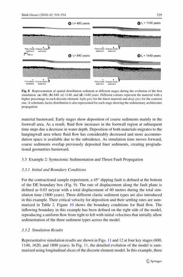
Fig. 8 Representation of spatial distribution sediment at different stages during the evolution of the firstsimulation: (a) 480, (b) 840, (c) 1140, and (d) 1440 years. Different colours represent the material with ahigher percentage in each discrete element: light grey for the finest material and deep grey for the coarsestone. A schematic facies distribution is also represented for each stage showing the sedimentary architecturepropagation

material basinward. Early stages show deposition of coarse sediments mainly in thefootwall area. As a result, fluid flow increases in the footwall region at subsequenttime steps due a decrease in water depth. Deposition of both materials migrates to thehangingwall area where fluid flow has considerably decreased and more accommo-dation space is available due to the subsidence. As simulation time moves forward,coarse sediments overlap previously deposited finer sediments, creating prograda-tional geometries basinward.

3.3 Example 2: Syntectonic Sedimentation and Thrust Fault Propagation

3.3.1 Initial and Boundary Conditions

For the contractional sample experiment, a 45◦ dipping fault is defined at the bottomof the DE boundary box (Fig. 9). The rate of displacement along the fault plane isdefined as 0.03 m/year with a total displacement of 60 metres during the total sim-ulation time (1800 years). Three different clastic sediment types are also introducedin this example. Their critical velocity for deposition and their settling rates are sum-marized in Table 2. Figure 10 shows the boundary conditions for fluid flow. Theinflowing boundary in this example has been defined on the right side of the model,reproducing a uniform flow from right to left with initial velocities that initially allowsedimentation of the three sediment types across the model.

3.3.2 Simulation Results

Representative simulation results are shown in Figs. 11 and 12 at four key stages (600,1140, 1620, and 1800 years). In Fig. 11, the detailed evolution of the model is sum-marized using longitudinal slices of the discrete element model. In this example, three

530 Math Geosci (2010) 42: 519–534

Fig. 9 Bounding box of the DE assemblage with a 45◦ dipping fault used in the second example. Thearrow shows the direction of the movement of the hangingwall area (uplifting region) with respect to thefootwall area

Fig. 10 Initial mesh and boundary conditions for water and sediment inflow used by Simsafadim-Clasticin the second simulation. The initial fluid flow field is also represented

Table 2 Sedimentationparameters used for the secondexperiment considering a thrustfault

Clastic 1 Clastic 2 Clastic 3

(fine) (medium) (coarse)

Critical velocity fordeposition (m s−1)

3.5 4.5 5.5

Settle rate(m day−1)

0.004 0.006 0.008

transfers of sediment volumes from Simsafadim-Clastic to the DE model take placeduring the evolution of the model. The four stages represented are immediately afterthese transfers of sediment (three first stages) and the model at the final simulationtime step (Fig. 11). The simulation results show how (as in the extensional example)sedimentation occurs during the first stage (600 years) in the inflowing region located

Math Geosci (2010) 42: 519–534 531

Fig. 11 Simulation results for the second simulation: (a) longitudinal cross-section of DEM; (b) syntec-tonic sedimentary geometries for four different stages. A fluid flow velocity map is also represented tofacilitate the comprehension of the evolution of the sedimentation

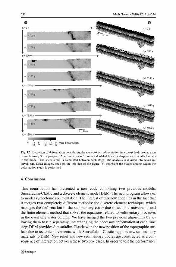
on the hangingwall and how the thickness of this sedimentation decreases basinward.In the next time steps, sedimentation migrates into the basin because of the waterdepth decrease and fluid flow velocity increase due to sedimentation and the upliftof the hangingwall region. Consequently, the locus of sedimentation is displaced tothe footwall region where accommodation space is still available. This results in aprogradation of sediments into the basin and a typical offlap geometry. Using themethodology developed by Cardozo and Allmendinger (2009), we can undertake adetailed analysis of the deformation in pre- and syn-sedimentary materials (Fig. 12).Maximum Shear Strain is calculated from the displacement of all elements in themodel. The shear strain is calculated between each stage. The represented time in-tervals in Fig. 12 have been chosen in order to show how the addition of the newsediments affects the evolution of the deformation in the model. Seven intervals havebeen selected: two for the time steps before the first transfer, two between each trans-fer, and a last one after the last transfer. The first two time intervals (up to 600 years)show how the propagation of deformation is concentrated above the fault zone wherea fault-propagation fold linked to a contractive system has been developed. After thefirst transfer of sediment from the Simsafadim-Clastic program, we can see that theupward propagation of the deformation is firstly inhibited owing to the weight of thenew material and is then reactivated after a period of time. This effect occurs when-ever new sediment is transferred and added, except during the seventh time intervalwhen this effect is not so evident because new sediment is deposited farther awayfrom the deforming region.

532 Math Geosci (2010) 42: 519–534

Fig. 12 Evolution of deformation considering the syntectonic sedimentation in a thrust fault propagationexample using SSPX program. Maximum Shear Strain is calculated from the displacement of all elementsin the model. The shear strain is calculated between each stage. The analysis is divided into seven in-tervals (a). DEM images, sited on the left side of the figure (b), represent the stages among which thedeformation study is performed

4 Conclusions

This contribution has presented a new code combining two previous models,Simsafadim-Clastic and a discrete element model DEM. The new program allows usto model syntectonic sedimentation. The interest of this new code lies in the fact thatit merges two completely different methods: the discrete element technique, whichmanages the deformation in the sedimentary cover due to tectonic movement, andthe finite element method that solves the equations related to sedimentary processesin the overlying water column. We have merged the two previous algorithms by al-lowing them to run separately, interchanging the necessary information at each timestep: DEM provides Simsafadim-Clastic with the new position of the topographic sur-face due to tectonic movements, while Simsafadim-Clastic supplies new sedimentarymaterials to DEM. New relief and new sedimentary bodies are constructed as a con-sequence of interaction between these two processes. In order to test the performance

Math Geosci (2010) 42: 519–534 533

of this new merged code, two example simulations that take into account sedimen-tation associated with the growth of a normal fault and a reverse fault are presented.Each example has been defined with a different set of initial and boundary conditionsfor fluid flow, transport, and sedimentation, as well as different tectonic boundaryconditions and displacement rates. Results obtained by both experiments show real-istic syntectonic stratigraphic architectures. The evolution of the basin topography inthe two examples is the result of both tectonic movements and sedimentation. Fluidflow and, consequently, transport and sedimentation change according to this evolv-ing topography. The depositional sedimentary bodies are similar to reported naturalexamples in each case. The transfer of sediments from Simsafim-Clastic to DEM al-lows us to have more realistic deformed sedimentary bodies as a result of the tectonicmovements occurring in a basin. It is also noted that the propagation of the deforma-tion is affected by the addition of syntectonic sediments into the model. The results ofboth experiments support the viability of the approach of combining the two models(i.e. Simsafadim-Clastic and DEM) and also the realism of model results. We canconclude that this new tool allows us to perform a more realistic and detailed studyof the way sedimentation and tectonics interact in nature.

Acknowledgements This research was carried out by the GEOMODELS Research Institute and theCRG Geodynamics and Basin Analysis (2001SGR_000074) of the University of Barcelona. This workwas supported by StatoilHydro (project 4D Modelling Based on Field Descriptions, project nr. 5348768)and the project MODES-4D (CGL2007-66431-CO”/BTE). The original manuscript has been improvedthanks to the valuable comments by Dr. Harff, an anonymous reviewer, and the guests’ editor, Jef Caers.

References

Allen MP, Tidsley DJ (1987) Computer simulations of liquids. Oxford Science Publications, OxfordAllmendinger RW (1998) Inverse and forward numerical modelling of trishear fault propagation folds.

Tectonics 17:640–656Bitzer K, Salas R (2002) SIMSAFADIM: three dimensional simulation of stratigraphic architecture and

facies distribution modelling of carbonate sediments. Comput Geosci 28:1177–1192Cardozo N, Allmendinger RW (2009) SSPX: a program to compute strain from displacement/velocity

data. Comput Geosci 35(6):1343–1357Cardozo N, Bawa-Bhalla K, Zehnder A, Allmendinger RW (2003) Mechanical models of fault propagation

folds and comparison to the trishear kinematic model. J Struct Geol 25:1–18Finch E, Hardy S, Gawthorpe R (2003) Discrete element modelling of contractional faults-propagation

folding above rigid basement rocks. J Struct Geol 25:515–528Finch E, Hardy S, Gawthorpe R (2004) Discrete element modelling of extensional faults-propagation

folding above rigid basement rocks. Basin Res 16:489–506Gawthorpe R, Hardy S (2002) Extensional fault-propagation folding and base-level changes as controls on

growth strata geometries. Sediment Geol 146:47–56Grajeon D, Joseph P (1999) Concepts and applications of a 3-D multiply lithology, diffusive model

in stratigraphic modelling. In: Harbaugh J, Watney W, Rankey E, Slingerland R, Goldstein R,Franseen E (eds) Numerical experiments in stratigraphy: recent advances in stratigraphic and sed-imentologic computer simulations. SEPM special publications, vol 62. Kansas Geological Survey,Lawrence, pp 197–210

Gratacós O (2004) Simsafadim-Clastic: modelización 3D de transporte y sedimentación Clástica Sub-acuática. Tesis doctoral, Universitat de Barcelona

Gratacós O, Bitzer K, Cabrera L, Roca E (2009a) SIMSAFADIM-CLASTIC: a new approach to mathemat-ical 3D forward simulation modelling for clastic and carbonate sedimentation. Geol Acta 7:311–322

Gratacós O, Bitzer K, Casamor JL, Cabrera L, Calafat A, Canals M, Roca E (2009b) Simulating trans-port and deposition of clastic sediments in an elongate basin using the SIMSAFADIM-CLASTICprogram: The Camarasa artificial lake case study (NE Spain). Sediment Geol 222(1–2):16–26

534 Math Geosci (2010) 42: 519–534

Hardy S (2008) Structural evolution of calderas: insights from two-dimensional discrete element simula-tions. Geol Soc Am 36(12):927–930

Hardy S, Finch E (2005) Discrete-element modelling of detachment folding. Basin Res 17:507–520Hardy S, Finch E (2006) Discrete element modelling of the influence of cover strength on basement-

involved fault-propagation folding. Tectonophysics 415:225–238Hardy S, Finch E (2007) Mechanical stratigraphy and the transition from trishear to kink-band fault-

propagation fold forms above blind basement thrust faults: a discrete-element study. Mar Pet Geol24:75–90

Hardy S, Gawthorpe R (1998) Effects of variations in fault slip rate on sequence stratigraphy in fan deltas.Mar Pet Geol 11(5):911–914

Hardy S, McClay K (1999) Kinematic modelling of extensional fault-propagation folding. J Struct Geol21:695–702

Hardy S, McClay K, Muñoz JA (2009) Deformation and fault activity in space and time in high-resolutionnumerical models of doubly vergent thrust wedges. Mar Pet Geol 26(2):232–248

Jin G, Groshong RH (2006) Trishear kinematic modeling of extensional fault-propagation folding. J StructGeol 28:170–183

Johnson KM, Johnson AM (2002) Mechanical models of trishear-like folds. J Struct Geol 24:277–287Kinzelbach W (1986) Groundwater modelling: an introduction with sample programs in BASIC. Elsevier,

AmsterdamLi M, Amos C (2001) SEDTRANS96: the upgraded and better calibrated sediment-transport model for

continental shelves. Comput Geosci 27:619–645Maniatis G, Kurfeß D, Hampel A, Heidbach O (2009) Slip acceleration on normal faults due to erosion

and sedimentation—Results from a new three-dimensional numerical model coupling tectonics andlandscape evolution. Earth Planet Sci Lett 284:570–582

Mora P, Place D (1993) A lattice solid model for the non-linear dynamics of earthquakes. Int J ModernPhys C 4(6):1059–1074

Mora P, Place D (1994) Simulation of the frictional stick-slip instability. Pure Appl Geophys 143(1–3):61–87

Simpson GDH (2006) Modelling interactions between fold-thrust belt deformations, foreland flexure andsurface mass transport. Basin Res 18:125–144

Simpson GDH (2009) Mechanical modelling of folding versus faulting in brittle-ductile wedges. J StructGeol 31:369–381

Strayer LM, Suppe J (2002) Out-of plane motion of a thrust sheet during along—strike propagation of athrust ramp: a distinct element approach. J Struct Geol 24:637–650

Tetzlaff DM, Harbaugh JW (1989) Simulating Clastic Sedimentation. Computer Methods in Geology.Van Nostrand and Reinhold, New York