i

Modelling Social Preferences of Ride-sharing

by

Ramandeep Singh Manjeet Singh Makhija

August 2108

A thesis submitted to the

faculty of the Graduate School of

the University at Buffalo, State University of New York

in partial fulfillment of the requirement for the

degree of

Master of Science

Department of Industrial and Systems Engineering

ii

Acknowledgements

I would like to express my gratitude for my thesis advisor, Dr. Qing He for

his support, guidance and patience constantly throughout my thesis. I would also

like to express my gratitude for my committee member Dr. Roger Chen for his

guidance and support. They were constantly guiding me whenever I had problems

or had some questions regarding my research or writing. I am thankful for their

encouragement and devotion that kept me stay devoted and focused on my research.

Finally, I would like to express my gratitude to my parents and friends for

their continuous encouragement and support throughout the process of research and

writing of my thesis. I couldn’t have been able to accomplish all this without them.

Thank you.

iii

Contents

Acknowledgements ii

List of Figures iv

List of Tables v

Abstract vi

1 Introduction 1

2 Literature Review 4

2.1 Non-survey-based approach . . . . . . . . . . . . . . . . . . . . . . . . . . . . . . . . . . . 4

2.2 Survey-based approach . . . . . . . . . . . . . . . . . . . . . . . . . . . . . . . . . . . . . . 5

3 Survey Design and Analysis 8

3.1 Data Preparation . . . . . . . . . . . . . . . . . . . . . . . . . . . . . . . . . . . . . . . . . . . . 8

3.2 Survey Methodology . . . . . . . . . . . . . . . . . . . . . . . . . . . . . . . . . . . . . . . . . 8

3.3 Analysis of the Survey . . . . . . . . . . . . . . . . . . . . . . . . . . . . . . . . . . . . . . . . 9

3.3.1 Demographics . . . . . . . . . . . . . . . . . . . . . . . . . . . . . . . . . . . . . . . 10

3.3.2 Education and Income . . . . . . . . . . . . . . . . . . . . . . . . . . . . . . . . . 11

3.3.3 Personality and personal preferences . . . . . . . . . . . . . . . . . . . . . 13

4 Methodology and Experimental Results 17

4.1 Data cleaning and preparation . . . . . . . . . . . . . . . . . . . . . . . . . . . . . . . . . 17

4.2 Factor Analysis . . . . . . . . . . . . . . . . . . . . . . . . . . . . . . . . . . . . . . . . . . . . . 20

4.3 Modelling Framework . . . . . . . . . . . . . . . . . . . . . . . . . . . . . . . . . . . . . . . . 23

4.4 Model Specification . . . . . . . . . . . . . . . . . . . . . . . . . . . . . . . . . . . . . . . . . . 24

4.4.1 Model 1: Organizational Latent Variable(Factor 1) . . . . . . . . . . . . 26

4.4.2 Model 2: Socioeconomic Latent Variable(Factor 2) . . . . . . . . . . . 27

4.4.3 Model 3: Drinking/Smoking Habit Latent Variable(Factor 3) . . . . . 29

4.4.4 Model 4: Socio-demographic Latent Variable(Factor 4) . . . . . . . . 30

4.5 Matching Index . . . . . . . . . . . . . . . . . . . . . . . . . . . . . . . . . . . . . . . . . . . . . 30

4.5.1 Numerical Example . . . . . . . . . . . . . . . . . . . . . . . . . . . . . . . . . . . . 33

5 Conclusion and Future Research Directions 35

5.1 Conclusion . . . . . . . . . . . . . . . . . . . . . . . . . . . . . . . . . . . . . . . . . . . . . . . . 35

5.2 Future Research Directions . . . . . . . . . . . . . . . . . . . . . . . . . . . . . . . . . . . 36

Bibliography 37

iv

List of Figures

1 Histogram of the first question gender response in percentages . . . . . . . . . . . . . . . 10

2 Distribution of age groups of responders in percentages . . . . . . . . . . . . . . . . . . . . . 10

3 Distribution of responders according to race in percentages . . . . . . . . . . . . . . . . . . 11

4 Distribution of the highest level of education completed by the responders. . . . . . . 11

5 Distribution of household income of the individual responders in percentages. . . . . 12

6 Modelling Frameworks . . . . . . . . . . . . . . . . . . . . . . . . . . . . . . . . . . . . . . . . . . . . . . . 23

v

List of Tables

1 The personality of responders in percentage of total responders. . . . . . . . . . . . . . . 13

2 Self-identified personal characteristics of respondents. . . . . . . . . . . . . . . . . . . . . . . 14

3 Preferences regarding rideshare passengers . . . . . . . . . . . . . . . . . . . . . . . . . . . . . . 15

4 Survey data variables – Personal attributes. . . . . . . . . . . . . . . . . . . . . . . . . . . . . . . . 18

5 Factor analysis results. . . . . . . . . . . . . . . . . . . . . . . . . . . . . . . . . . . . . . . . . . . . . . . . 21

6 Model estimation results. . . . . . . . . . . . . . . . . . . . . . . . . . . . . . . . . . . . . . . . . . . . . 28

7 Calculated similarities between riders A, B and C for all factors. . . . . . . . . . . . . . . . 33

8 Calculated preference probabilities for rider A for all factors. . . . . . . . . . . . . . . . . . . 33

9 Matching Index between A, B and C for all factors . . . . . . . . . . . . . . . . . . . . . . . . . . 34

vi

Abstract

Ride-sharing also known as carpooling is sharing of journeys from one place to another so

that more than one person can travel together and obviate others from driving to the locations

themselves. By having more than one people sharing a vehicle, ride sharing avails to reduce

personal expenses such as fuel, driving stress and tolls. The objective of this paper is to

model the social preferences of people ride-sharing together i.e. to identify challenges

and barriers people face to adopt ride-sharing and model their social preferences to obtain the final

prediction for probabilities. First from the literature problems and challenges were identified which

people face to adopt ride-sharing. Then a questionnaire was created as a survey which was

conducted among the citizens of the United States to know the preferences and attributes of the

ride-sharers. Further, using the data collected from the survey, a discrete mode choice analysis

was performed. There were 13 main latent variables used for modeling. These 13 variables were

grouped into four factors using factor analysis. Finally, four models were created

using ordinal logistic regression to predict the probabilities of a person enjoying his/her shared

rides in social aspects from his attributes and preferences. After the estimation of 4 final models

we estimated a matching index using preference probabilities from the models that give a

compatibility ratio between riders.

Keywords: ride-sharing behavior; survey; social preferences; ordinal logistic regression; factor

analysis; latent variables.

vii

Dedicated to my family and friends . . .

1

Chapter 1

Introduction

Ride-sharing also called as carpooling is sharing of journeys from one place to another so that

more than one person can travel together and obviate others from driving to the locations

themselves. By having more than one people sharing a vehicle, ride sharing avails to reduce

personal expenses such as fuel, driving stress and tolls. It additionally avails reducing pollution,

gaseous emissions like carbon, traffic on roads and desideratum of parking spaces. Ride-sharing

additionally has potentials to increment social capital as it lets different people meet and know

each other. Ride-sharing is thereby considered as environment-friendly and sustainable way of

traveling.

As mentioned in most of the previous studies ride sharing is considered an efficient way to reduce

road traffic, pollution, etc. for any country, business, or an individual. However, ride-sharing can

struggle to be flexible to accommodate changes in times and working patterns. According to one

of the survey, flexibility was the most common reason for not ride-sharing (19). As stated by (1)

in their paper there are three main issues people face to adopt ride sharing – trust, awareness,

inconvenience, and availability. They conducted a survey to understand the issues people face to

2

adopt ridesharing. Based on the results and analysis of their survey they proposed to design a

system for dynamic ride-sharing which will incorporate all these issues.

Ride-sharing has not been adopted very commonly. There are many systems in the form of bulletin

board-like websites that facilitate the match between drivers and passengers. The driver announces

the number of empty sets in his vehicle many days before he is going to travel. Then the passengers

and the driver’s coordinate with each other through the website, private messages or email. This

is a static way of ride-sharing. In this case, there can be many social barriers or problems between

the passenger and the driver as there is no way to get the social compatibility between them. Also,

very few ride-sharing platforms have taken into account travelers’ social attributes and ride

discomfort with strangers for their matching algorithms. Accordingly, knowing the social barriers

and trying to match driver and passenger as per their preferences will lead to an increase in

adoption of ride-sharing. This was the main motivation of the study to social barriers that restrict

people to adopt ride-sharing.

The main objective of this study is to identify the challenges and social barriers people actually

face to adopt ride sharing. It also aims to identify significant factors that lead people to not adopt

ride sharing and to identify one’s social preference in choosing ride-sharer.

The objective is achieved by conducting a survey among the citizens of US asking them about the

challenges they face to adopt ride sharing. Using the result of the survey a model was created to

identify significant factors and to predict the probability of compatibility between people ride

sharing together.

3

Following are the steps undertaken in this study:

Identifying major problems and challenges people face to adopt ride sharing from the

literature.

Creating a questionnaire for the survey to be taken using the problems and challenges

identified.

Conducting the survey among citizens of US and getting the responses for further analysis.

Factor analysis of the responses to group down all 13 latent variable responses into four

different factors.

Using the survey results to create discrete choice models to identify significant factors.

Then four different models were created using logistic regression with latent variables.

Then using the preference probabilities from the model a matching index was calculated

which gives the compatibility ratio between riders.

4

Chapter 2

Literature Review

We classify the literature in ride-sharing behavior into two categories: Non-survey-based approach

and Survey based approach which are as follows:

2.1 Non-survey-based approach

There are many methods that were used to improve adoption of ride sharing. One of them is

through combining ride sharing with social network. Wessel, R. proposed a web system that

combines with social network which will tend to improve trust and security (3). The factors

considered are friendliness, safety, and reliability. The results showed such that about 23% of

people are willing to lose more time to pick up a friend rather than a stranger which is 6%.

The paper (7) by Gidofalvi, G. et al. considered maximization of social connections to improve

adoption of ride sharing. The author tried to reduce the social discomfort and safety risks which

5

are associated with ride sharing. Users are connected to each other by a social network data source.

The number of short paths between two users tells us about the strength of the connection between

them. But the issues of the adoption of ride-sharing were not taken into account.

Another study (8) proposed a system which divides passenger route into different small segments

which are part of other trips, called as dynamic multi-hop system. This paper also considered the

social aspects, like matching drivers and passengers by linking the application with social networks

such as Facebook etc. and matching the user profiles.

The paper (5) reported on the HOV (High Occupancy Vehicles) lane and suggested no fees for

HOV’s on bridges. The author also suggested giving priority to female passengers by not leaving

them alone for a longer duration waiting for a ride considering safety. There were some suggestions

provided by the author for future research which includes safety and reputation system design i.e.

authenticating users before matching.

2.2 Survey-based approach

Survey is an unbiased approach to take decisions in any research. As said by Wyse in (11) that the

four reasons why businesses and researchers should conduct surveys are that surveys help uncover

answers about any research, give your survey respondents an opportunity to discuss important key

topics, base decision on objective information and help provide information like thoughts,

comments and opinions about the target audience of the survey. Survey for ride-sharing research

is also conducted to know what difficulties people face to adopt ride sharing.

6

As given in paper (12) by Ayele and Byun, to understand personal, social psychological and other

factors affecting ridesharing programs, they designed a “Ride-sharer survey”. They analyzed this

survey considering two different aspects of which one involved general statistics and other was a

cooperative statistical analysis in which they grouped ride-sharers in different groups (by income,

age, sex, and race etc.). The results from this research were compared to identify how these

variables affect ride sharing.

Horowtiz (13) gave significant importance to study of the role of psychological attitude in

ridesharing. He came up with a framework in which attitudes, beliefs affecting behavioral

intention, can affect ridesharing. He hypothesized that everyone has a set of positive and negative

evaluation about ridesharing. Also, he developed a mathematical model of ridesharing to explore

how advantages and disadvantages of ridesharing determine behavioral tendency.

As mentioned by Burkhardt and Millard-Ball in (16), innovativeness and pro-environmental

attitudes are recognized as the common characteristic among the ridesharing users. Schaefers in

his research (18) also identified social innovativeness and pro-environmental considerations with

two other motivational patterns which are thriftiness and convenience as the underlining patterns

for ride-sharing use. Kopp et al. in his research (17) suggested that ridesharing users are more

likely to exhibit multi-modal travel patterns which were also corroborated by Schaefers (18) in his

work.

Krueger, Rashidi, and Rose (14) studied the travel behavior impacts, by identifying willingness

and characteristics of users who are more likely to adopt Sports activity vehicle (SAV). A survey

was conducted and analyzed using a logit model. The results of the research in (14) convey that

7

the service attribute can be critical determinants of SAV and ridesharing acceptance. The uptake

of ridesharing and SAV will differ across different population groups, and the set modes may be

considered as an important determinant of subgroup membership.

As stated in (15), shared vehicles are the vehicles that serve several people throughout a day. There

are more than 25 ride-sharing companies that already exist but people still face issues to adopt ride

sharing.

From the literature, it can be seen that the major problems and challenges people face to adopt ride

sharing are psychological factors like trust, compatibility etc. Although a number of studies have

been conducted to identify these factors and tries to improve the adaptability of ride sharing. Our

study aims to improve the adaptability by identifying factors as well as checking the compatibility

between people who want to ride share together. Having the compatibility ratio before even ride

sharing with someone will help to improve the adaptability. In this study, a survey-based approach

is devised and the methodology used for model creation and predicting the probability is similar

to the choice model from the study of Bierlaire (22).

8

Chapter 3

Survey Design and Analysis

3.1 Data Preparation

A survey was designed and distributed among national residents of USA through the paid service

provided by Survey Monkey. This survey was intended to know the influence of the social,

psychological and other personal factors on ridesharing. The main objective of this survey was:

to determine challenges that people face to adopt ride-sharing;

to obtain attitudinal data indicating social preference in ride-sharing;

to determine impacts of personal demographics to prospective riders.

3.2 Survey Methodology

The survey questionnaires contained 9 different questions which include personal demographics

and also questions to determine challenges that people face to adopt ride-sharing.

9

The main questions asked in the survey included questions about demographics, personal

characteristics, and what kind of people one would like to ride share with. First five questions were

about demographics and personal questions like age group, gender, race, income, etc. The sixth

question asked people to tell about themselves. The seventh question was about the major or

expertise. Eight question was to know if a person smokes, drinks, likes shopping, like to be on

social media, etc. The ninth question contained 13 different sub-questions asking the preferences

of people about the ones they would like to ride share with. For example, “who as similar income

as I do?”, “who has the same gender as I do?”, etc. The response to the ninth question was as a

latent response with seven levels from “strongly disagree” to “strongly agree”. In this manner, 273

responses to the survey were collected for further analysis.

3.3 Analysis of the survey

The analysis of this survey focused on the analysis of general characteristics and a comparative

and statistical analysis in which people were grouped by income, age, race, gender, education level,

major or expertise.

Statistical analysis of survey responses is explained as follows:

10

3.3.1 Demographics:

Figure 1: Histogram of the first question of gender response in percentages

As seen in Figure 1, there were 53.68% of male responders, 45.59% of the female responders and

the rest 0.74% were who preferred not to disclose their gender.

Figure 2: Distribution of age groups of responders in percentages

As seen in Figure 2, the responders for the survey were all distributed in different age groups. The

highest number of responders was from age group “21-29 years” (31.62% of the total responders)

and the lowest number of responders were from the age group “18-20 years” (5.68% of total).

11

Figure 3: Distribution of responders according to race in percentage.

From Figure 3, it can be seen that the highest number of responders for our survey were “White”,

i.e 73.53% of the total responders and least were “American Indian or Alaskan Native” and “Native

Hawaiian or other Pacific Islander” i.e. 0.74% of the total responders for the both.

3.3.2 Education and Income:

Figure 4: Distribution of the highest level of education completed by the responders.

From Figure 4, it can be seen that more than 50% of the responders had a bachelor degree or

higher, and more than 70% of the responders pursued degree higher than high school or equivalent.

12

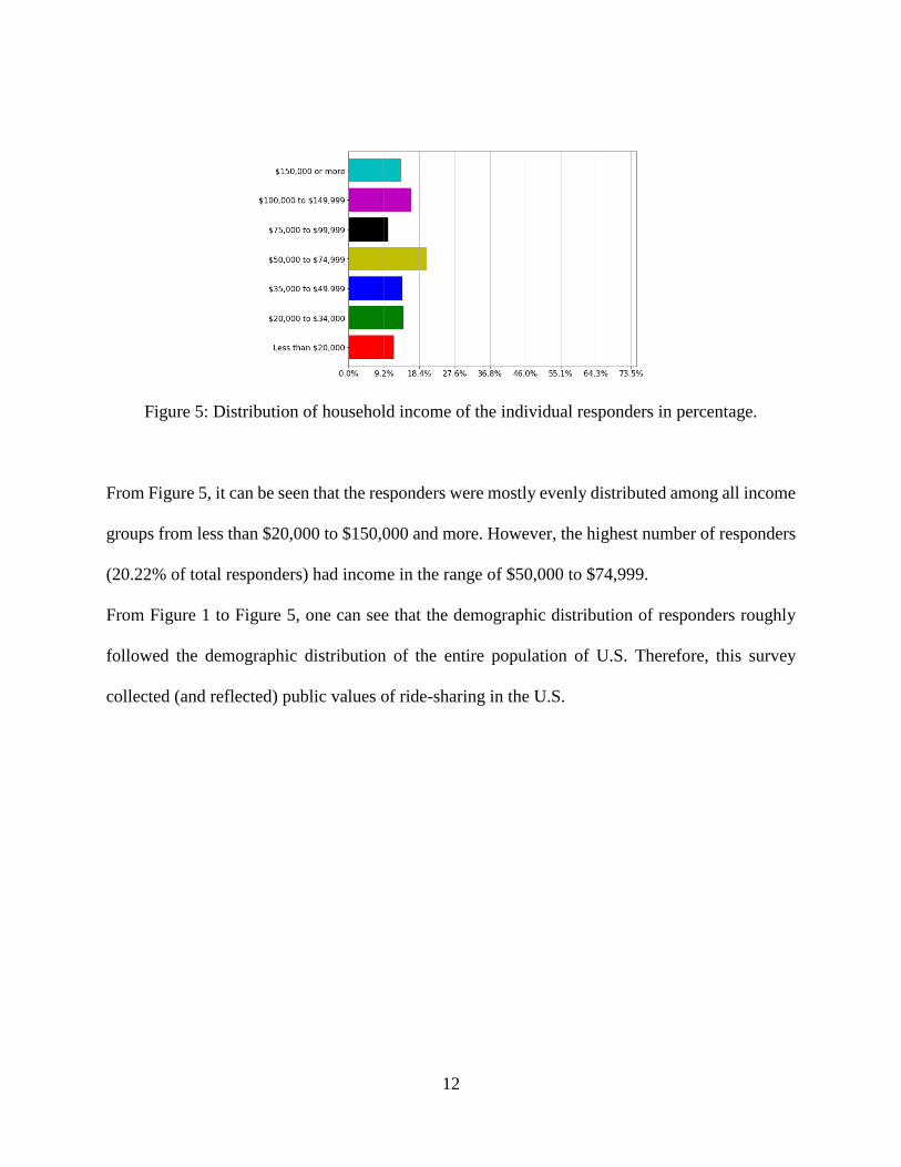
Figure 5: Distribution of household income of the individual responders in percentage.

From Figure 5, it can be seen that the responders were mostly evenly distributed among all income

groups from less than $20,000 to $150,000 and more. However, the highest number of responders

(20.22% of total responders) had income in the range of $50,000 to $74,999.

From Figure 1 to Figure 5, one can see that the demographic distribution of responders roughly

followed the demographic distribution of the entire population of U.S. Therefore, this survey

collected (and reflected) public values of ride-sharing in the U.S.

13

3.3.3 Personality and personal preferences:

Table 1: The personality of responders in percentage of total responders.

Answer Choices Responses

I see myself as: Extraverted, enthusiastic. 28.68%

I see myself as: Critical, quarrelsome. 11.76%

I see myself as: Dependable, self-disciplined. 51.47%

I see myself as: Anxious, easily-upset. 14.71%

I see myself as: Open to new experiences, complex. 45.26%

I see myself as: Reserved, quiet. 37.13%

I see myself as: Sympathetic, warm. 44.12%

I see myself as: Disorganized, careless. 8.46%

I see myself as: Calm, emotionally stable. 38.60%

I see myself as: Conventional, unreactive. 9.56%

Total respondents: 272

From Table 1, it can be seen that most responders have described themselves to be “Dependable,

self-disciplined”, “Open to new experiences, complex”, “Sympathetic, warm”, “Reserved, quit”,

etc. The least number of responders have described themselves as “Disorganized, careless”,

“Conventional, unreactive”, etc.

14

Table 2: Self-Identified personal characteristics of respondents

Answer Choices Responses

Smokes sometimes 15.81%

Drink Sometimes 60.29%

Like to go shopping 41.18%

Play a musical instrument 25.00%

Like going out for eating sometimes 83.82%

Like watching movies 76.47%

Like to be on social media 42.65%

Go out for parties, get-together, outings etc. sometimes 47.06%

Go on a vacation trip sometimes 76.84%

Play sports sometimes 36.40%

Like outdoor activities like trekking, hiking etc. 56.25%

Total Respondents: 272

From Table 2, it can be seen that most responders are interested in going out for eating, watching

movies, vacation and are cool with drinking occasionally. There were very fewer responders who

responded that they were okay with smoking sometimes. The average percentage of responders,

about 30% to 50%, responded that they would like to be on social media, go out to parties, play

sports sometimes, like to go shopping, etc.

15

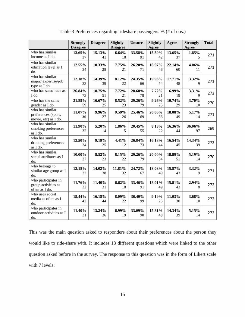
Table 3 Preferences regarding rideshare passengers. % (# of obs.)

Strongly

Disagree

Disagree Slightly

Disagree

Unsure Slightly

Agree

Agree Strongly

Agree

Total

who has similar

income as I do. 13.65%

37 15.13%

41

6.64%

18 33.58%

91 15.50%

42

13.65%

37 1.85%

5 271

who has similar

education level as I

do.

12.55%

34

10.33%

28

7.75%

21

26.20%

71

16.97%

46

22.14%

60

4.06%

11 271

who has similar

major/ expertise/job

type as I do.

12.18%

33

14.39%

39

8.12%

22

24.35%

66

19.93%

54

17.71%

48

3.32%

9 271

who has same race as

I do. 26.84%

73

18.75%

51

7.72%

21

28.68%

78

7.72%

21

6.99%

19

3.31%

9 272

who has the same

gender as I do. 21.85%

59

16.67%

25

8.52%

23

29.26%

79

9.26%

25

10.74%

29 3.70%

10 270

who has similar

preferences (sport,

movie, etc) as I do.

11.07%

30

9.96%

27

9.59%

26

25.46%

69

20.66%

56

18.08%

49

5.17% 14

271

who has similar

smoking preferences

as I do.

11.90% 32

5.20%

14

1.86%

5

20.45%

55

8.18%

22

16.36%

44

36.06%

97 269

who has similar

drinking preferences

as I do.

12.50%

34

9.19%

25

4.41%

12

26.84%

73

16.18%

44

16.54%

45

14.34%

39 272

who has similar

social attributes as I

do.

10.00%

27 8.52%

23

8.15%

22

29.26%

79

20.00%

54

18.89%

51

5.19%

14 270

who belongs to

similar age group as I

do.

12.18%

33

14.02%

38

11.81%

32

24.72%

67

18.08%

49

15.87%

43

3.32%

9 271

who participates in

group activities as

often as I do.

11.76%

32 11.40%

31

6.62%

18

33.46%

91

18.01%

49

15.81% 43

2.94%

8 272

who uses social

media as often as I

do.

15.44%

42

16.18%

44

8.09%

22

36.40%

99

9.19%

25

11.03%

30 3.68%

10 272

who participates in

outdoor activities as I

do.

11.40%

31

13.24%

36 6.99%

19

33.09%

90 15.81%

43

14.34%

39

5.15%

14 272

This was the main question asked to responders about their preferences about the person they

would like to ride-share with. It includes 13 different questions which were linked to the other

question asked before in the survey. The response to this question was in the form of Likert scale

with 7 levels:

16

1. strongly disagree,

2. disagree,

3. slightly disagree,

4. unsure,

5. slightly agree,

6. agree, and

7. strongly agree.

From Table 3, it can be seen that responders cared more about the smoking, drinking and social

attributes with and the least they cared about was the demographic characteristics about the people

they want to ride-share with.

17

Chapter 4

Methodology and Experimental Results

In order to characterize the relationship between responses to ride-sharing preferences (i.e. “I

prefer to rideshare with someone who has similar drinking habits.”) and other rider attributes a

model of latent variables that inform multiple observed ordinal choices (attitudinal Likert scale

statements) was estimated with the survey data. This section presents the model formulation and

estimation results, including discussion and interpretation results. The next section discusses the

data cleaning and preparation, followed by the model formulation.

4.1 Data Cleaning and Preparation

Before using the survey response for model estimation, the original Likert scale responses were

collapsed to a 3-item scale (1-disagree, 2-unsure, 3-agree). The motivation for this was to provide

item levels with a reasonable number of observations each. Other variables used as covariates to

explain the response to Likert scale items include (i) personal socio-demographics; (ii) general

preferences and hobbies (i.e. like shopping, playing musical instruments, etc.); and (iii) self-

identified personality traits (i.e. quarrelsome, extroverted, anxious, etc.). Additionally, respondents

18

indicated preferences for ride-sharing passengers through a series of attitudinal Likert scale

statements. These variables and items are listed and described next. The personal attributes of

respondents from the survey are listed and described in Table 4.

Table 4: Survey data variables - personal attributes

Name Description

AGE

Age group range: 1 = 18 to 20 years, 2 = 21 to 29 years, 3 = 30 to 39 years,

4 = 40 to 49 years, 5 = 50 to 59 years, and 6 = 60 years+.

GENDER Gender: 1 = Male, 2 = Female, 3 = N/A

RACE

Ethnicity origin (or Race): 1 = White, 2 = Black/African-American, 3 =

American Indian/Alaskan native, 4 = Asian, 5 = Native Hawaiian/other

Pacific Islander, 6 = From multiple races, and 7 = Other

EDUCATION

Highest level of Education: 1 = Less than high school degree, 2 = High

degree or equivalent, 3 = Some college but no degree, 4 = Associate degree,

5 = Bachelor degree, 6 = Graduate degree, and 7 = PhD

INCOME

Household Income Range for 2016: 1 = Less than $20,000, 2 = $20,000 to

$34,999, 3 = $35,000 to $49,000, 4 = $50,500 to $74,999, 5 = $75,000 to

$99,999, 6 = $100,000 to $149,999, and 7 = $150,000 or more.

SMOKES 1 = Smokes; 0 = Does not Smoke

DRINKS 1 = Drinks Alcohol; 0 = Does not Drink Alcohol

19

Self-Identified Descriptors: Additionally, binary responses were collected from respondents

indicating if the following statements properly characterized or described themselves; variable

names are in parentheses:

Likes Shopping (SHOP)

Plays a Musical Instrument (MUSIC)

Likes Watching Movies (MOVIES)

Likes using Social Media (SMEDIA)

Likes Parties (PARTY)

Likes Vacations (VACATION)

Plays Sports (SPORTS)

Extroverted/Enthusiastic (EXTROVERT)

Critical/Quarrelsome (CRITICAL)

Dependable/Self-Disciplined (DEPENDABLE)

Anxious/Easily Upset (ANXIOUS)

Open to new Experiences/Complex (OPEN)

Reserved/Quiet (QUIET)

Sympathetic/Warm (WARM)

Disorganized/Careless (CARELESS)

Calm/Emotionally Stable (CALM)

Conventional/Uncreative (UNCREATIVE)

Passenger Preference Responses: Finally, respondents were asked to respond to 3-item Likert

Scale attitudinal statements regarding the type of passengers with whom they prefer to ride-share

20

with. These statements are listed below with variable names in parentheses. The three levels are:

1 = disagree; 2 = unsure and 3 = agree. For example, if the respondent answered "1" to "Income

Level," they disagree that they would like to ride with similar income level passengers.

Income Level (S_INCOME)

Education Level (S_EDU)

College Major (S_MAJOR)

Race (S_RACE)

Gender (S_GENDER)

Preferences (sports teams, watching movies, etc.) (S_PREF)

Smoking Habits (S_SMOKE)

Drinking Habits (S_DRINK)

Social Habits/Attributes (S_SOCIAL)

Age (S_AGE)

Participation in Group Activities (parties, etc.) (S_GROUP)

Use of Social Media (S_SOCIALMEDIA)

Outdoor Activities (i.e. trekking, hiking, etc.) (S_OUTDOOR)

4.2 Factor Analysis

The survey dataset contained 13 multi-item Likert scale questions regarding preferences for ride-

share passengers described above. In order to distill these responses into latent variables that

characterize the response to these 13 questions, a factor analysis was conducted to reveal the

21

number of latent variables needed to explain the majority of variation in responses. An ordinal

logit joint among groups of statements was estimated for each of the resulting latent factors. A

factor analysis for M= 3, 4, 5, 6 factors was completed to identify the appropriate number of latent

factors. Based on the chi-square statistic for the model with two and three factors (M=2, 3), the

factor analysis model with M=3 had a lower test-statistic and higher p-value, indicating preference

over the M=2 factor model. Based on chi-square test statistic for the model with 4 factors (M=4),

at, was preferred. We accept the hypothesis that four factors sufficiently explain the variance.

Additionally, the Eigenvalues (SS loadings) indicate the amount of variance is accounted for each

of four factors. Factors with high SS loadings reflect their significance for explaining variances in

responses. A “rule of thumb” is an SS loadings value greater than 1, to indicate importance (25).

All factors in the four-factor model have SS loadings greater than 1.

Table 5: Factor analysis results

Likert Scale Attitudinal Statement Factor 1 Factor 2 Factor 3 Factor 4

Similar Income (S_INCOME) --- 0.648 --- ---

Similar Education (S_EDU) --- 0.817 --- ---

Similar Major (S_MAJOR) --- 0.600 --- ---

Similar Race (S_RACE) --- --- --- 0.609

Similar Gender (S_GENDER) --- --- --- 0.741

Similar Preferences (S_PREF) 0.550 --- --- ---

Similar Smoking (S_SMOKE) --- --- 0.645 ---

Similar Drinking (S_DRINK) --- --- 0.790 ---

Similar Social (S_SOCIAL) 0.555 --- --- ---

Similar Age (S_AGE) 0.575 --- --- ---

Similar Participation (S_GROUP) 0.854 --- --- ---

Similar Social Media Use (S_SOCIALMEDIA) 0.605 --- --- ---

Similar Outdoor Activities (S_OUTDOOR) 0.681 --- --- ---

Factor 1 Factor 2 Factor 3 Factor 4

SS loadings 2.901 2.016 1.511 1.351

Proportion Variance 0.223 0.155 0.166 0.104

Cumulative Variance 0.223 0.378 0.494 0.598

22

Interestingly four factors (M=4) emerged that aligned with different groups of statements. The

latent variables or factors from the factor analysis were interpreted as follows:

Factor 1 (Organizational): Indicates preference for similar social or organizational

engagement; this latent variable captures variance in responses to these statements: (i)

Similar Preferences, (ii) Similar Social Habits, (iii) Similar Age, (iv) Similar Participation,

(v) Similar use of Social Media; and (vi) Similar Outdoor activities.

Factor 2 (Socioeconomic): Indicates preference for similar socioeconomic characteristics

(i.e. education, household income); this latent variable captures variance in responses to

these statements: (i) Similar Income; (ii) Similar Education; and (iii) Similar Major.

Factor 3 (Social Habits): Indicates preference for similar drinking and smoking habits; this

latent variable capture response variance to: (i) Similar Smoking Habits; and (ii) Similar

Drinking Habits.

Factor 4 (Socio-Demographic): Indicates preference for similar socio-demographics (i.e.

gender, race, etc.); this latent variable capture response variance to: (i) Similar Race and

(ii) Similar Gender.

23

4.3 Modeling Framework

Given the identified latent factors, we use an ordered response model representing each latent

factor to investigate the relationship between survey responses and latent factors. Latent variables

which are unobserved but measurable through responses to indicators arise frequently in the

transportation and marketing literature. Our framework models the four types of preferences as

latent variables. The data used for estimating these models were from an intercept survey that

collected responses to attitudinal measurement indicators and other respondent information. The

final model specification is a model of the latent constructs, with Likert scale responses as

indicators. The entire model system is shown below in Figure 6. Latent variables and indicators

all have measurement and other errors indicated as ɛs and ɛM respectively. The main components

of the modeling framework in Figure 5 are as follows:

Figure 6: Modeling Framework for ordered logit model.

Explanatory Variables (X): These include observed attributes of the survey respondent. These are

all collected through the survey developed.

Latent Variables (𝑋∗): These are the four latent preferences towards ride-share passengers.

24

Attitudinal and Perceptual Indicators (I): These consist of respondent ratings towards statements

regarding the dimensions of ride-share passengers that are latent and psychological. The marketing

field has long developed scales that evaluate latent consumer perceptions (26). The list of

indicators collected is given in Table 5.

4.4 Model Specification

Given the theoretical concepts, this section provides the model specifications for the four latent

variables. This latent variable was modeled based on responses to 13 Likert scale indicator

responses, of which only 11 were found to be statistically significant in the final four model

specifications. The structural equation was specified as follows:

𝑋∗ = 𝛽0𝑆 + 𝛽1

𝑆𝑋1 + 𝛽2𝑆𝑋2 + ⋯ + 𝛽𝐾

𝑆𝑋𝐾 + 𝜎𝑠휀𝑆 (Eq. 1)

𝑋∗ a latent variable, in this case one of the four ride-share preferences

𝑋 a vector of explanatory variables, observed and/or unobserved

𝛽𝑆 a vector of parameters to be estimated from the data

휀𝑆 a random error term, which is assumed to be Gumbel distributed

𝜎𝑠 scale parameter of 휀𝑆

The measurement equation 𝑍 that related the latent variable 𝑋∗ to the observed responses to

indicators I was specified as follows:

25

𝐼𝑖 = 𝑓(𝑥) = {

𝑗1, 𝑋∗ < 𝑘1

𝑗2, 𝑘1 ≤ 𝑋∗ < 𝑘2

𝑗3, 𝑘2 ≤ 𝑋∗ (𝐸𝑞. 2)

𝑋∗ a latent variable, in this case, one of the four ride-share preferences

𝐼𝑖 response to an indicator statement, such as an attitudinal statement i=1 to 13

This paper has three measurement levels M=3 in Eq. 6. For each Likert response, we define two

parameters 𝜏𝑖 and 𝛿𝑖 that define the thresholds 𝑘𝑖 as follows:

𝑘1 = 𝜏𝑖 (Eq. 3)

𝑘2 = 𝜏𝑖 + 𝛿𝑖 (Eq. 4)

In the final model specification for the four latent variables, only 2-4 of the original i=1..13 Likert

scale indicators were found statistically significant per factor. This was also indicated in the factor

analysis in Table 5. The final specification for each latent model had the following equations:

a) 1 structural, for the single latent variable (Factor 1, Factor 2, Factor 3 or Factor 4) (Eq. 1)

b) 2-4 measurement equations, for each indicator retained (Eq. 2)

Given the Gumbel assumptions of the error term, probabilities of the particular ordinal choice of

Likert scale level given a latent variable (Factors 1 to 4) is:

𝑃𝑟(𝑎𝑔𝑟𝑒𝑒) =1

1+exp (−(𝑋∗+𝑘1)) (Eq. 5)

26

𝑃𝑟(𝑢𝑛𝑠𝑢𝑟𝑒) =1

1+exp (−(𝑋∗+𝑘2))− 𝑃𝑟(𝑎𝑔𝑟𝑒𝑒) (Eq. 6)

𝑃𝑟(𝑑𝑖𝑠𝑎𝑔𝑟𝑒𝑒) = 1 − 𝑃𝑟(𝑎𝑔𝑟𝑒𝑒) − 𝑃𝑟(𝑢𝑛𝑠𝑢𝑟𝑒) (Eq. 7)

The final likelihood function for the observed sample is:

𝐿𝑛(𝐼|𝑋; 𝛽𝑠, 𝜏, 𝛿𝑖,Σ) = ∫ ∏ 𝑃𝑟(𝐼𝑟 = 𝑗𝑖𝑛|휀𝑠)𝑅𝑟=1 ∙ 𝑑휀𝑠𝜀𝑠

(Eq.8)

We estimate the final model using Full Information Maximum Likelihood (FIML) using the

likelihood function in Eq. 12. The model was implemented and estimated in BIOGEME (21) an

open-source freeware designed for the maximum likelihood estimation of parametric models in

general, with a special emphasis on discrete choice models. The trust region method was used as

the optimization algorithm to solve the maximum likelihood estimation problem. Next, we discuss

the estimation results for the four models estimated.

4.4.1 Model 1: Organizational Latent Variable (Factor 1):

From Table 6, three person-level attributes were statistically significant in explaining the first

latent variable characterizing organizational preferences (Factor 1). First, the variable ANXIOUS

had a negative sign. If the respondent self-characterized him/herself as “anxious,” this had a

negative impact on the thresholds for the ordinal logit model, indicating these individuals tend to

disagree preference for passengers with similar social and other organizational activities. The

27

positive sign on UNCREATIVE indicates that individuals who were conventional or uncreative

tend to agree with these statements, indicating a high preference for passengers with similar

organizational attitudes. Finally, the respondent with household incomes less than $50,000

annually tends to prefer passengers with similar organizational attitudes. Second, the threshold

parameter estimates (τ and δ) were similar for all four attitudinal statements (OUTDOOR,

GROUP, PREF and SOCIAL). This indicates that controlling for all other factors, in general

individuals responded to the 3-item Likert scales for these dimensions similarly.

4.4.2 Model 2: Socioeconomic Latent Variable (Factor 2):

For Model 2, Table 6 indicates the same three person-level attributes significant in explaining

Model 1 were also significant for explaining the second latent variable characterizing

socioeconomic preferences (Factor 2). Similarly, the variable ANXIOUS also had a negative sign

indicating a negative impact on the thresholds for the ordinal logit model. Similar to Model 1,

respondents who were self-described as “anxious” tend to disagree with the associated attitudinal

statements. UNCREATIVE and INCOME both had similar effects to Model 1. Turning attention

again to the threshold parameter estimates (τ and δ), these were similar for all THREE attitudinal

statements (INCOME, EDU, and MAJOR). The thresholds for MAJOR were slightly more

negative relative to the other two dimensions, indicating in general slightly more disagreement

with that attitudinal statement.

28

Table 6: Model estimation results

Parameter Value t-statistic P-value Value t-statistic P-value Value t-statistic P-value Value t-statistic P-value

Threholds for Joint Ordinal Logit Model

δ for S_OUTDOOR 1.420 10.690 0.000 --- --- --- --- --- --- --- --- ---

τ for S_OUTDOOR -0.595 -3.740 0.000 --- --- --- --- --- --- --- --- ---

δ for S_GROUP 1.460 10.930 0.000 --- --- --- --- --- --- --- --- ---

τ for S_GROUP -0.685 -4.290 0.000 --- --- --- --- --- --- --- --- ---

δ for S_PREF 1.100 9.260 0.000 --- --- --- --- --- --- --- --- ---

τ for S_PREF -0.627 -3.920 0.000 --- --- --- --- --- --- --- --- ---

δ for S_SOCIAL 1.310 10.120 0.000 --- --- --- --- --- --- --- --- ---

τ for S_SOCIAL -0.863 -5.280 0.000 --- --- --- --- --- --- --- --- ---

δ for S_INCOME --- --- --- 1.150 9.490 0.000 --- --- --- --- --- ---

τ for S_INCOME --- --- --- -0.655 -4.230 0.000 --- --- --- --- --- ---

δ for S_EDU --- --- --- 1.470 10.920 0.000 --- --- --- --- --- ---

τ for S_EDU --- --- --- -0.436 -2.920 0.000 --- --- --- --- --- ---

δ for S_MAJOR --- --- --- 1.030 9.010 0.000 --- --- --- --- --- ---

τ for S_MAJOR --- --- --- -0.469 -3.090 0.000 --- --- --- --- --- ---

δ for S_DRINK --- --- --- --- --- --- 1.250 9.490 0.000 --- --- ---

τ for S_DRINK --- --- --- --- --- --- -0.880 -4.740 0.000 --- --- ---

δ for S_SMOKE --- --- --- --- --- --- 1.070 7.970 0.000 --- --- ---

τ for S_SMOKE --- --- --- --- --- --- -1.330 -6.830 0.000 --- --- ---

δ for S_GENDER --- --- --- --- --- --- --- --- --- 1.360 10.000 0.000

τ for S_GENDER --- --- --- --- --- --- --- --- --- -0.365 -1.580 0.110

Respondent Personal Attributes

β for ANXIOUS = 1 -0.618 -2.740 0.010 -0.447 -1.580 0.030 -0.629 -2.190 0.030 --- --- ---

β for UNCREATIVE = 1 0.842 3.730 0.000 1.120 3.320 0.000 1.520 3.610 0.000 --- --- ---

β for INCOME = 1, 2, 3, 4: $0-$50,000 0.545 2.870 0.000 0.408 2.050 0.040 --- --- --- --- --- ---

β for OPEN = 1 --- --- --- --- --- --- -0.383 -1.810 0.050 -0.477 -1.960 0.050

β for GENDER = 2 (Female) --- --- --- --- --- --- 0.791 3.280 0.000 --- --- ---

β for RACE = 4 (Asian) --- --- --- --- --- --- --- --- --- 9.510 2.330 0.020

β for RACE = 5 (Native Hawaiian/other Pacific Islander) --- --- --- --- --- --- --- --- --- 0.844 4.350 0.000

β for QUIET --- --- --- --- --- --- --- --- --- 0.447 1.920 0.050

β for GENDER = 1 (Male) --- --- --- --- --- --- --- --- --- -0.552 -2.360 0.020

Summary Statistics

Number of Observations

Log-likelihood (0) - No Parameters

Log-likelihood at Convergence -279.046-523.888

273 273

-1293.485

-1163.164

-987.467

-872.500

Model 1: Organizational

Latent Variable

Model 2: Socioeconomic

Latent Variable

Model 3: Drinking/Smoking

Latent Variable

Model 4: Sociodemographic

Latent Variable

273

-621.043

273

-487.670

29

4.4.3 Model 3: Drinking/Smoking Habits Latent Variable (Factor 3):

In Model 3, the estimation results in Table 6 indicate different personal attributes that impact the

latent variable characterizing riders who prefer passengers with similar drinking and making

habits. For this model a total of four personal attributes were significant. In addition to respondents

self-characterizing themselves as anxious (ANXIOUS) and conventional (UNCREATIVE), being

open to new experiences (OPEN) and female (GENDER = 2) also had statistically significant

impacts. Interestingly, being open to new experiences had a negative impact on the thresholds,

indicating they tend to disagree more with respect to these two attitudinal statements, relative to

other respondents. One possible explanation could be that respondents open to new experiences

tend to have stronger opinions and more readily disagree. Self-identifying as a female led to higher

threshold values, as indicated by the positive coefficient on GENDER=2. Both ANXIOUS and

UNREACTIVE had similar signs to Models 1 and 2.

With respect to the thresholds, the τ for SMOKE was more negative than DRINK. This indicates

that on average, respondents tend to agree with ridesharing with passengers with similar drinking

habits more relative to smoking. This seems reasonablile since smoking has a more direct

consequence on passengers than drinking (you share the same space as smoke or its odors.).

30

4.4.4 Model 4: Socio-demographic Latent Variable (Factor 4):

Finally, looking at Model 4 the personal attributes impacting the thresholds for Model 4 were quite

different from the other three models. In the case of the last model, RACE, being reserved (QUITE)

and being male (GENDER=1) appear to significantly impact this latent factor. If the respondent

identified as Asian or Native Hawaiian, the impact of the threshold increased, indicating a higher

likelihood of individuals agreeing that they would prefer passengers with a similar race. Asian and

Native Hawaiian respondents tend to prefer ridesharing with similar race passengers. The same

holds true for individuals identifying as reserved (QUIET=1); these individuals prefer riding with

other passengers with similar race. Interestingly, identifying as Asian has a much higher positive

impact relative to others, indicating extreme preference for similar race passengers. Both being

open to new experiences (OPEN=1) and male (GENDER=1) had negative impacts on threshold

values. Respondents identifying as either do not prefer to rideshare with similar race passengers.

Interestingly, observed responses to the statement of preferring passengers of similar gender

(S_GENDER=1) had no significant impact on the model likelihood at convergence and was not

included. The thresholds for Model 4 were similar to those for the other three models.

4.5 Matching Index

Using the preference probabilities calculated from equations 5, 6, and 7, a matching index for

ranking riders with other riders with a high probability of matching preferences is calculated. The

maching index gives a compatibility ratio between two riders.

31

Matching index can be calculated in three steps for any rider pair A and B respectively:

1. First calculate similarity between the riders you are considering for matching:

Similarity between A and B can be given by:

𝑆𝑖𝐴𝐵 = ∑ 𝜃𝑗𝑥𝑗

𝐴𝐵𝑗 (Eq.9)

where, 𝑖 = 1, 2, 3, 4 (all factors)

𝜃𝑗 = 𝑛𝑜𝑟𝑚𝑎𝑙𝑖𝑧𝑒𝑑 𝑣𝑎𝑙𝑢𝑒𝑠 𝑜𝑓 𝑜𝑟𝑖𝑔𝑖𝑛𝑎𝑙 𝑣𝑎𝑟𝑖𝑎𝑏𝑙𝑒 𝑗 𝑓𝑟𝑜𝑚 𝑓𝑎𝑐𝑡𝑜𝑟 𝑎𝑛𝑎𝑙𝑦𝑠𝑖𝑠 𝑓𝑜𝑟 𝑓𝑎𝑐𝑡𝑜𝑟 𝑖

∑ 𝜃𝑗 = 1𝑗

𝑥𝑗𝐴𝐵 = 1 𝑖𝑓 𝐴 𝑎𝑛𝑑 𝐵 ℎ𝑎𝑣𝑒 𝑠𝑖𝑚𝑖𝑙𝑎𝑟 𝑗 𝑎𝑛𝑑 0 𝑜𝑡ℎ𝑒𝑟𝑤𝑖𝑠𝑒.

We need the similarity between riders to get a value that can be used in the further equation

to calculate matching index. This will be used as a coefficient to be multiplied with the

probability of agreement to get a value which lies between [0, 1]. It is a multiplication of

normalized values 𝜃𝑗 and 𝑥𝑗𝐴𝐵 . As both the value lie between [0, 1] the multiplication will

result in values between [0, 1].

2. Now we calculate the matching index as follows:

𝑀𝐴/𝐵𝑖 = 𝑌3𝐴

𝑖 + (𝑌1𝐴𝑖 × 𝑆𝑖

𝐴𝐵) + (𝛾 × 𝑌2𝐴𝑖 ) (Eq.10)

where, 𝑌1𝐴𝑖 = 𝑝𝑟𝑜𝑏𝑎𝑏𝑖𝑙𝑖𝑡𝑦 𝑜𝑓 𝑎𝑔𝑟𝑒𝑒 𝑜𝑓 𝑝𝑒𝑟𝑠𝑜𝑛 𝐴 𝑓𝑜𝑟 𝑓𝑎𝑐𝑡𝑜𝑟 𝑖 𝑓𝑟𝑜𝑚 𝐸𝑞. 5

𝑌2𝐴𝑖 = 𝑝𝑟𝑜𝑏𝑎𝑏𝑖𝑙𝑖𝑡𝑦 𝑜𝑓 𝑢𝑛𝑠𝑢𝑟𝑒 𝑜𝑓 𝑝𝑒𝑟𝑠𝑜𝑛 𝐴 𝑓𝑜𝑟 𝑓𝑎𝑐𝑡𝑜𝑟 𝑖 𝑓𝑟𝑜𝑚 𝐸𝑞. 6

𝑌3𝐴𝑖 = 𝑝𝑟𝑜𝑏𝑎𝑏𝑖𝑙𝑖𝑡𝑦 𝑜𝑓 𝑑𝑖𝑠𝑎𝑔𝑟𝑒𝑒 𝑜𝑓 𝑝𝑒𝑟𝑠𝑜𝑛 𝐴 𝑓𝑜𝑟 𝑓𝑎𝑐𝑡𝑜𝑟 𝑖 𝑓𝑟𝑜𝑚 𝐸𝑞. 7

𝑆𝑖𝐴𝐵 = 𝑆𝑖𝑚𝑖𝑙𝑎𝑟𝑖𝑡𝑦 𝑏𝑒𝑡𝑤𝑒𝑒𝑛 𝐴 𝑎𝑛𝑑 𝐵 𝑓𝑟𝑜𝑚 𝐸𝑞. 9

𝛾 = 0.6, 𝑓𝑎𝑐𝑡𝑜𝑟 𝑐𝑜𝑛𝑠𝑖𝑑𝑒𝑟𝑒𝑑 𝑓𝑜𝑟 𝑡ℎ𝑖𝑠 𝑡ℎ𝑒𝑠𝑖𝑠 𝑓𝑜𝑟 𝑎 𝑝𝑒𝑟𝑠𝑜𝑛 𝑏𝑒𝑖𝑛𝑔 𝑢𝑛𝑠𝑢𝑟𝑒

From Eq. 10, we can see that matching index was calculated by summation of three

probabilities multiplied with their coefficients. To get a matching index which has a value

32

between [0, 1] we made sure that all the three summation factors had values between [0,

1]. This equation was considered as it incorporated all three preference probabilities of the

riders. 𝑌3𝐴𝑖 is the preference probability of disagreement for factor 𝑖 of rider A. As this

probability is for disagreement so it will directly affect matching index and there is no need

of any coefficient for this. 𝑌2𝐴𝑖 is the preference probability of a person being unsure about

factor 𝑖. So it has to be multiplied by a coefficient 𝛾, which is selected to be as 0.6 for this

study. 𝑌1𝐴𝑖 is the preference probability of agreement for factor 𝑖 of rider A. So, it is

multiplied by a similarity index which is calculated in Eq. 9, So summation of all these

preference probabilities multiplied with their coefficients gives us the matching index for

a particular factor 𝑖. So the final value of the matching index for a particular factor 𝑖 lies

between [0, 1].

3. Aggregating 4 factor matching index to single matching index:

𝑀𝐴/𝐵 = ∑ ∝𝑖 𝑀𝐴/𝐵𝑖

𝑖 (Eq.11)

where, ∝𝑖= 𝑤𝑒𝑖𝑔ℎ𝑡𝑎𝑔𝑒 𝑜𝑓 𝑒𝑎𝑐ℎ 𝑓𝑎𝑐𝑡𝑜𝑟 𝑖

The weightage ∝𝑖 can be considered as same or different based upon the estimation. It

can also be taken according to the number of statements grouped together by factor

analysis. More the number of statements in a factor more will be the weightage. For this

study we have considered all factors to have equal weightage so the Eq. 11 becomes as

follows.

𝑀𝐴/𝐵 = ∝ ∑ 𝑀𝐴/𝐵𝑖

𝑖 (Eq.12)

where, ∝ = 0.25 𝑎𝑠 𝑎𝑙𝑙 𝑓𝑎𝑐𝑡𝑜𝑟𝑠 𝑎𝑟𝑒 𝑐𝑜𝑠𝑖𝑑𝑒𝑟𝑒𝑑 𝑤𝑖𝑡ℎ 𝑠𝑎𝑚𝑒 𝑤𝑒𝑖𝑔ℎ𝑡𝑎𝑔𝑒

33

4.5.1 Numerical example:

Consider three people A, B and C with following attributes:

A: male, Asian, conventional unreactive, Income less than $50,000, open to new experiences,

reserved/quiet, drinks sometimes but doesn’t smokes, have bachelor’s degree or equivalent.

B: male, Asian, anxious and easily upset, conventional/unreactive, Income in the range $50, 000

to $99,000, open to new experiences, reserved/quiet, drinks and smokes sometimes, have

bachelor’s degree or equivalent.

C: female, Native Hawaiian, conventional unreactive, Income less than $50,000, open to new

experiences, reserved/quiet, drinks and smokes sometimes, have bachelor’s degree or equivalent.

Therefore, using Eq. 9, the similarities are as follows:

Table 7: Calculated similarities between riders A, B and C for all factors.

Organizational (Factor 1)

Socio-economic (Factor 2)

Social Habits (Factor 3)

Socio-demographic (Factor 4)

𝑺𝒊𝑨𝑩 1 0.397 0.55 1

𝑺𝒊𝑨𝑪 1 0.721 0.55 0

Now the preference probabilities for A from Eq’s. 5, 6, and 7 is calculated as:

Table 8: Calculated preference probabilities for rider A for all factors.

Organizational (Factor 1)

Socio-economic (Factor 2)

Social Habits (Factor 3)

Socio-demographic (Factor 4)

𝒀𝟏𝑨𝒊 0.673 0.732 0.513 0.99

𝒀𝟐𝑨𝒊 0.209 0.169 0.227 0.009

𝒀𝟑𝑨𝒊 0.118 0.099 0.088 0.001

34

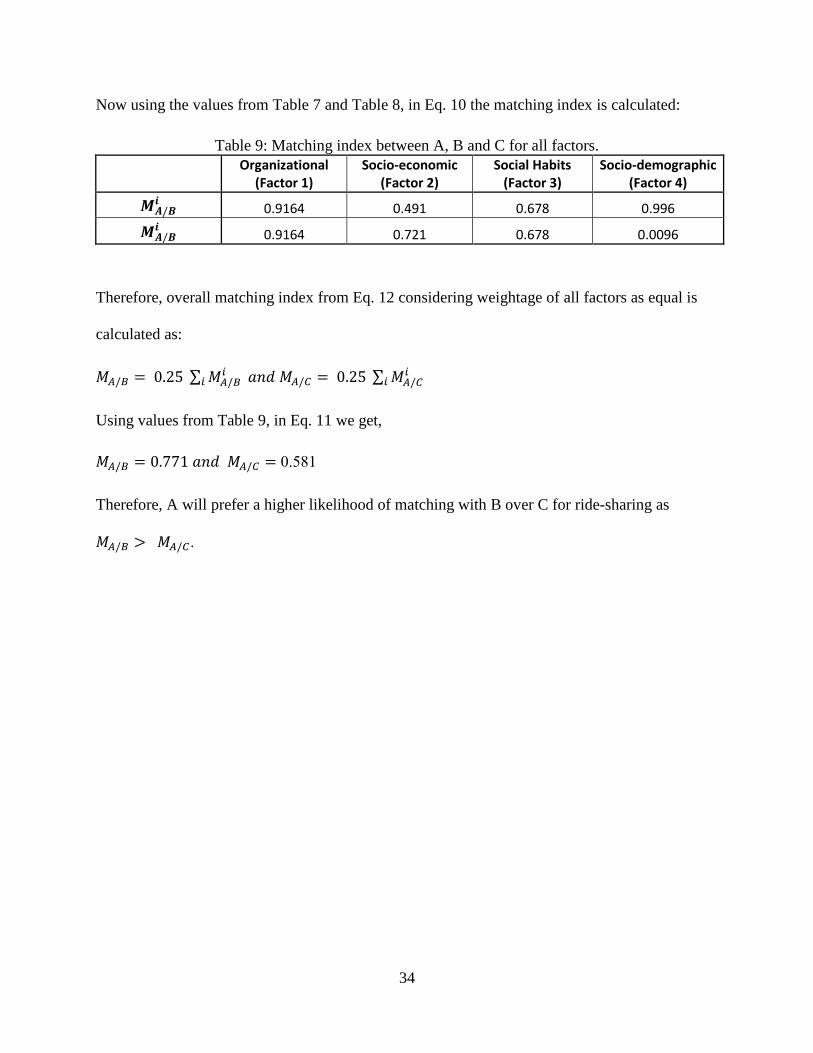
Now using the values from Table 7 and Table 8, in Eq. 10 the matching index is calculated:

Table 9: Matching index between A, B and C for all factors.

Organizational (Factor 1)

Socio-economic (Factor 2)

Social Habits (Factor 3)

Socio-demographic (Factor 4)

𝑴𝑨/𝑩𝒊 0.9164 0.491 0.678 0.996

𝑴𝑨/𝑩𝒊 0.9164 0.721 0.678 0.0096

Therefore, overall matching index from Eq. 12 considering weightage of all factors as equal is

calculated as:

𝑀𝐴/𝐵 = 0.25 ∑ 𝑀𝐴/𝐵𝑖

𝑖 𝑎𝑛𝑑 𝑀𝐴/𝐶 = 0.25 ∑ 𝑀𝐴/𝐶𝑖

𝑖

Using values from Table 9, in Eq. 11 we get,

𝑀𝐴/𝐵 = 0.771 𝑎𝑛𝑑 𝑀𝐴/𝐶 = 0.581

Therefore, A will prefer a higher likelihood of matching with B over C for ride-sharing as

𝑀𝐴/𝐵 > 𝑀𝐴/𝐶.

35

Chapter 5

Conclusion and Future Research Directions

5.1 Conclusion

This study examines the social preferences of ride-sharing passengers for other passengers. A

factor analysis of Likert scale attitudinal statements on these preferences uncovered four latent

factors. We interpreted these factors as Organizational (Factor 1), Socioeconomic (Factor 2),

Smoking/Drinking Habits (Factor 3), and Sociodemographic (Factor 4). For each of these four

factors, a joint ordered logit model was estimated based on the responses to statements that grouped

together from the factor analysis. The estimated models revealed interesting relationships between

the respondent attributes and preferences for rideshare passengers.

First, individuals with anxiety tend to prefer riding with similar type passengers with respect to (i)

organizational activities; (ii) socioeconomics and (iii) drinking/smoking habits. Anxious

individuals who self-identify as quarrelsome with others intuitively would not prefer to ride with

anyone in general, let alone passengers with similar characteristics. Conventional individuals who

36

do not experiment much not surprisingly prefer passengers with similar preferences. Conversely

individuals who are open to new experiences do not prefer passengers with similar

smoking/drinking habits or similar races. With respect to preference for similar race rideshare

passengers, Model 4 indicated Asians have the highest preference for similar race passengers,

followed by Native Hawaiians and those that self-identify as quiet and introspective. The model

estimation did not reveal significant gender differences for preferring similar race and

drinking/smoking habits. Both males and female responded negatively to these statements.

Further a matching index was computed using the preference probabilities from the estimated

models. Matching index gave us the compatibility ratio between riders. Riders with high matching

index will have a higher chance of ride-sharing together. A numerical example was taken into

consideration with three riders A, B and C. As 𝑀𝐴/𝐵 > 𝑀𝐴/𝐶, A has higher chances of ride-

sharing with B than he has with C.

5.2 Future Research Directions

Future work includes incorporating more preferences and model estimates to give a good

estimation. Data can be collected on larger scale for the analysis and estimation. Improvement in

calculation of matching index can be done like getting different weights for different factors while

calculating aggregated matching index and also we can have some way to validate matching index.

37

Bibliography

1. V. Chaube, A.L. Kavanaugh, M.A. Perez-Quinones “Leveraging Social Networks to

Embed Trust in Rideshare Programs”, Proceeding of the 43rd Hawaii International

Conference on System Sciences – 2010.

2. Mayer, R. C., Davis, J. H. and Schoorman F. D., “An Integrative Model of Organizational

Trust”, The Academy of Management Review (20) 3, 1995, pp. 709-734.

3. Wessels, R. Combining Ridesharing & Social Networks. Technical report (2009),

http://www.aida.utwente.nl/education/ITS2-RW-Pooll.pdf

4. An Analysis of issues against the adoption of Dynamic Carpooling Daniel Graziotin, Free

University of Bozen-Bolzano, daniel.graziotin@unibz.it December 2010

5. Resnick, P. SocioTechnical support for ride sharing. In Working Notes of the Symposium

on Crossing Disciplinary Boundaries in the Urban and Regional Contex (UTEP-03) (2006).

6. Morse, J., Palay, J., Luon, Y., and Nainwal, S.“CarLoop: leveraging common ground to

develop long-term carpools”, CHI’07 Extended Abstracts on Human Factors in Computing

Systems Factors in Computing Systems, San Jose, CA, May 2007, pp. 2073-2078.

7. Gidófalvi, G. et al. Instant Social Ride-Sharing. In Proc. 15th World Congress on

Intelligent Transport Systems, p 8, Intelligent Transportation Society of America (2008)

8. Gruebele, P.A., Interactive System for Real Time Dynamic Multi-hop Carpooling. Global

Transport Knowledge Partnership (2008).

38

9. Kirshner, D. Pilot Tests of Dynamic Ridesharing. Technical report (2006),

http://www.ridenow.org/ridenow_summary.html

10. Gregory Albiston, Taha Osman, Evtim Peytchev – “Modelling Trust in Semantic Web

Applications”. (2015)

11. Defranzo, Susan E.: "The 4 main reasons to Conduct Surveys". Written on June 29, 2012.

https://www.snapsurveys.com/blog/4-main-reasons-conduct-surveys

12. Mooges, A. and Joon B., Personal, Social, Psychological and Other Factors in Ridesharing

Programs, U.S Department of Transportation. (1985)

13. Horowtiz, Abraham D., Ridesharing to work: a psychological analysis, University of

Illinois at Urbana-Champaign. (1976)

14. R. Krueger, T. H. Rashidi and J. M. Rose, Preferences for Shared autonomous vehicles,

Transportation Research Part C 69 (2016) 343-355

15. Burns, L.D., 2013. A vision for our transport future. Nature 497, 181–182.

http://dx.doi.org/10.1038/497181a.

16. Burkhardt, J.E., Millard-Ball, A., 2006. Who is attracted to carsharing? Transp. Res. Rec.

J. Transp. Res. Board 1986, 98–105.

17. Kopp, J., Gerike, R., Axhausen, K.W., 2015. Do sharing people behave differently? An

empirical evaluation of the distinctive mobility patterns of free-floating car-sharing

members. Transportation 42, 449–469. http://dx.doi.org/10.1007/s11116-015-9606-1.

18. Schaefers, T., 2013. Exploring carsharing usage motives: a hierarchical means-end chain

analysis.Transp. Res. Part A: Policy Pract. 47, 69–77.

39

19. Li, Jianling, Embry, Patrick, Mattingly, Stephen P., Sadabadi Kaveh Farokhi, Rasmidatta

Isaradatta, and Burris Mark W. Who Chooses to Carpool and Why? Examination of Texas

Carpoolers. Transportation Research Record, 2007.

20. Chan, Nelson D. & Shaheen, Susan A. (2012): Ridesharing in North America: Past,

Present, and Future, Transport Reviews, 32:1, 93-112.

21. Oliphant, Marc & Amey, Andrew. Dynamic Ridesharing: Carpooling Meets the

Information Age. 2010.

22. Bierlaire, Michael, Estimating choice models with latent variables with PythonBiogeme,

2016.

23. Bierlaire, M. (2016) PythonBiogeme: a short introduction. Report TRANSP-OR 160706,

Series on Biogeme. Transport and Mobility Laboratory, School of Architecture, Civil and

Environmental Engineering, Ecole Polytechnique Fédérale de Lausanne, Switzerland.

24. Shaheen, Susan A. and Cohen, Adam P. (2007): Growth in Worldwide Carsharing: An

International Comparison, Transportation Research Record, Vol 1992, Issue 1, pp. 81 – 89

25. Thomas G. Relo Jr., Brad Shuck (2014): "Exploratory Factor Analysis: Implications for

Theory, Research and Practice.

26. Bearden, W. O. and Netemeyer, R. G. (1999) Handbook of Marketing Scales, 2nd Edition,

Sage Publications.