University of Wollongong University of Wollongong

Research Online Research Online

Faculty of Science, Medicine and Health - Papers: part A Faculty of Science, Medicine and Health

1-1-2014

Modelling plant species distribution in alpine grasslands using airborne Modelling plant species distribution in alpine grasslands using airborne

imaging spectroscopy imaging spectroscopy

Julien Pottier University of Lausanne

Zbynek Malenovký University of Wollongong, zbynek@uow.edu.au

Achilleas Psomas Swiss Federal Research Institute WSL

Lucie Homolova University of Zurich

Michael E. Schaepman University of Zurich

See next page for additional authors

Follow this and additional works at: https://ro.uow.edu.au/smhpapers

Part of the Medicine and Health Sciences Commons, and the Social and Behavioral Sciences

Commons

Recommended Citation Recommended Citation Pottier, Julien; Malenovký, Zbynek; Psomas, Achilleas; Homolova, Lucie; Schaepman, Michael E.; Choler, Philippe; Thuiller, Wilfried; Guisan, Antoine; and Zimmermann, Niklaus E., "Modelling plant species distribution in alpine grasslands using airborne imaging spectroscopy" (2014). Faculty of Science, Medicine and Health - Papers: part A. 2257. https://ro.uow.edu.au/smhpapers/2257

Research Online is the open access institutional repository for the University of Wollongong. For further information contact the UOW Library: research-pubs@uow.edu.au

Modelling plant species distribution in alpine grasslands using airborne imaging Modelling plant species distribution in alpine grasslands using airborne imaging spectroscopy spectroscopy

Abstract Abstract Remote sensing using airborne imaging spectroscopy (AIS) is known to retrieve fundamental optical properties of ecosystems. However, the value of these properties for predicting plant species distribution remains unclear. Here, we assess whether such data can add value to topographic variables for predicting plant distributions in French and Swiss alpine grasslands. We fitted statistical models with high spectral and spatial resolution reflectance data and tested four optical indices sensitive to leaf chlorophyll content, leaf water content and leaf area index. We found moderate added-value of AIS data for predicting alpine plant species distribution. Contrary to expectations, differences between species distribution models (SDMs) were not linked to their local abundance or phylogenetic/functional similarity. Moreover, spectral signatures of species were found to be partly site-specific. We discuss current limits of AIS-based SDMs, highlighting issues of scale and informational content of AIS data.

Keywords Keywords species distribution, reflectance, hyperspectral data, alpine grasslands

Disciplines Disciplines Medicine and Health Sciences | Social and Behavioral Sciences

Publication Details Publication Details Pottier, J., Malenovsky, Z., Psomas, A., Homolova, L., Schaepman, M. E., Choler, P., Thuiller, W., Guisan, A. & Zimmermann, N. E. (2014). Modelling plant species distribution in alpine grasslands using airborne imaging spectroscopy. Biology Letters, 10 (7), 1-4.

Authors Authors Julien Pottier, Zbynek Malenovký, Achilleas Psomas, Lucie Homolova, Michael E. Schaepman, Philippe Choler, Wilfried Thuiller, Antoine Guisan, and Niklaus E. Zimmermann

This journal article is available at Research Online: https://ro.uow.edu.au/smhpapers/2257

Title: 1

MODELLING PLANT SPECIES DISTRIBUTION IN ALPINE GRASSLANDS USING 2

AIRBORNE IMAGING SPECTROSCOPY. 3

4

Authors: 5

Julien Pottier1,2, Zbyněk Malenovský3,4, Achilleas Psomas5, Lucie Homolová3, Michael E. 6

Schaepman3, Philippe Choler6,7,8, Wilfried Thuiller6,7*, Antoine Guisan1*, and Niklaus E. 7

Zimmermann5* 8

9

Authors’ affiliation: 10

1Department of Ecology and Evolution, Biophore 1015, Lausanne, Switzerland 11

2INRA, UR874, F-63100, Clermont-Ferrand, France 12

3Remote Sensing Laboratories, University of Zürich, 8057 Zürich, Switzerland 13

4School of Biological Sciences, University of Wollongong, Northfields Ave, NSW 2522, 14

Australia 15

5Swiss Federal Research Institute WSL, 8903 Birmensdorf, Switzerland 16

6Univ. Grenoble Alpes, LECA, F-38000 Grenoble, France 17

7CNRS, LECA, F-38000 Grenoble, France 18

8Station Alpine Joseph Fourier, UMS CNRS-UJF 3370, Univ. Grenoble Alpes F-38041, 19

Grenoble Cedex 9, France 20

* shared last authorship 21

22

Number of figures: 2 23

24

Electronic supplementary material: 25

ESM1: Details on data acquisition, processing and modelling. 26

ESM2: Complementary results. 27

28

Abstract: 29

Remote sensing using airborne imaging spectroscopy (AIS) is known to retrieve fundamental 30

optical properties of ecosystems. However, the value of these properties for predicting plant 31

species distribution remains unclear. Here, we assess whether such data can add value to 32

topographic variables for predicting plant distributions in French and Swiss alpine grasslands. 33

We fitted statistical models with high spectral and spatial resolution reflectance data and 34

tested four optical indices sensitive to leaf chlorophyll content, leaf water content and leaf 35

area index. We found moderate added-value of AIS-data for predicting alpine plant species 36

distribution. Contrary to expectations, differences between species distribution models were 37

not linked to their local abundance or phylogenetic/functional similarity. Moreover, spectral 38

signatures of species were found to be partly site-specific. We discuss current limits of AIS-39

based species distribution models, highlighting issues of scale and informational content of 40

AIS-data. 41

42

Keywords: 43

species distribution, reflectance, hyperspectral data, alpine grasslands. 44

45

1. INTRODUCTION 46

Spatial modelling of species distributions is commonly used to forecast environmental change 47

effects, detect biodiversity hotspots or predict species’ invasions [1]. As fine-grained 48

environmental descriptors are difficult to obtain, coarse-grained (from hundred of metres to 49

kilometres) topo-climatic descriptors are usually used. Recent advances in airborne imaging 50

spectroscopy (AIS) have allowed the acquisition of images with high spectral and sub-metre 51

spatial resolution [2]. Spectral information provided by remotely-sensed reflectance is 52

influenced by phenology, variations in morphological, structural and biochemical properties 53

of species [3], as well as by local environmental conditions (e.g. hydric stress, soil properties 54

or productivity [4,5]) that determine species habitat suitability [6]. Nevertheless, previous 55

attempts to predict species distributions with hyperspectral data have generated mixed results 56

[7,8]. Sub-metre resolution allows the targeting of small plants and micro-habitats where 57

species find refuge, highlighting potential benefits of hyperspatial remote sensing for 58

biodiversity monitoring [9]. However, despite increased spatial and spectral resolution of 59

airborne data, little is known about its value in modelling species’ distributions in species-rich 60

ecosystems characterised by fine-scale heterogeneity. 61

Here, we explore the predictive power of AIS-data for modelling plant species distributions in 62

alpine grasslands in two distinct regions. Specifically, we aim to: i) identify key remotely-63

sensed spectral information for predicting the distribution of grassland species; and ii) assess 64

whether AIS-data substantially improves model predictions. We also test for any phylogenetic 65

or functional dependency of model characteristics among species. 66

67

2. MATERIAL AND METHODS 68

(a) Study sites and species data 69

The study was conducted in the Western French (FR) and Western Swiss (CH) Alps (Electronic 70

Supplementary Material (ESM) 1). The French site included 103 vegetation plots of 2-5m in radius, 71

located between 2000 and 2830 metres above sea level (m.a.s.l.). The Swiss site included 68 quadrats 72

(2 by 2 m) located between 1650 and 2150 m.a.s.l. Species cover was visually estimated using the 73

Braun-Blanquet abundance scale. In total 160 species were selected for species distribution analysis 74

(119 species in FR, 78 in CH). Thirty-seven species were common to both sites (see ESM 1 for the 75

details on selection criteria). 76

77

(b) Remote sensing data 78

AIS-data were acquired with the dual Airborne Imaging Spectroradiometer for Applications (AISA; 79

Specim Ltd., Finland). Raw AISA images contained 359 spectral bands between 400 and 2450 nm 80

with spectral resolution ranging from 4.3 to 6.3 nm, and a pixel size of 0.8 m. After image processing, 81

we extracted two types of AIS-predictors: i) reflectance in 75 spectral bands (avoiding bands with 82

noisy radiometric response), and ii) four vegetation indices. Vegetation indices characterized leaf 83

chlorophyll (TCARI/OSAVI and ANCB) [10], leaf water content (SIWSI) [11] and leaf area index 84

(MTVI2) [12] (for details see ESM 1). Removal of poorly-vegetated plots resulted in datasets with 70 85

FR and 53 CH plots. 86

87

(c) Topographic predictors 88

We computed five predictors derived from digital elevation models at 50 m resolution for FR and 25 89

m resolution for CH, representing meso-scale habitat conditions : i) elevation (metre), ii) slope 90

(degree), iii) aspect (degree), iv) topographic position index (unitless), and v) topographic wetness 91

index (unitless) (see ESM 1). 92

93

(d) Species distribution modelling 94

Species distribution models (SDMs) were fitted with five different sets of variables: i) topographic 95

predictors only, ii) reflectance predictors only, iii) vegetation indices only, iv) topographic and 96

reflectance predictors combined, and v) topographic predictors and vegetation indices combined. We 97

first used a conditional Random Forest algorithm to estimate the unbiased relative importance of 98

predictors in the case of multi-colinearity, then ran final models based on selection of the most 99

important predictors [13] (see ESM 1). Their predictive accuracy was evaluated within each study site 100

separately using a repeated split-sample procedure (100 iterations). 70% of the sample points were 101

used for model calibration and 30% for model evaluation in each iteration. 102

103

(e) Model differences among species 104

The relative importance of AIS-predictors and the predictive accuracy of SDMs were tested against 1) 105

species’ phylogenetic relatedness, 2) species’ functional similarity, including a set of morphological 106

and physiological traits that are well correlated with the reflectance of canopy stands [14] (see ESM 2, 107

section 5), and 3) species’ abundance patterns within plots. Phylogenetic and functional tests were 108

computed as described in [15] (see ESM 2, section 5). 109

110

3. RESULTS 111

When fitting SDMs with reflectance data the analysis of predictor importance indicated 112

similarities in the selected spectral bands among sites (Figure 1). The most important spectral 113

bands were located between 500 and 900 nm for both sites, but site-specific differences in 114

important spectral bands were also apparent (1500-1800 nm in FR, 1200-1500 nm and 2000-115

2500 nm in CH). These site differences existed for species present at only one or both sites 116

(ESM 2, Figure 1). On average, all vegetation indices showed similar importance for SDM 117

fitting (ESM 2, Figure 2). 118

The prediction accuracy of SDMs based solely on topographic predictors, reflectance data or 119

vegetation indices did not differ significantly. However, SDMs including both AIS and 120

topographic predictors tended to be more accurate (Figure 2 and ESM 2, Table 1). The 121

improvement was marginally significant for vegetation indices (Wilcoxon rank sum test, p 122

=0.079) but non-significant for reflectance in FR. Conversely, CH showed significant 123

improvement when using reflectance (Wilcoxon rank sum test, p = 0.012), but non-significant 124

effects when using vegetation indices. Improvements when including AIS-predictors differed 125

among species, with few species showing ≥10% improved predictions and many showing 126

reduced predictive accuracy (ESM 2, Figure 3). These variations were independent of species’ 127

abundance patterns and species’ phylogenetic or functional similarity (ESM 2, Figures 4-13). 128

129

4. DISCUSSION 130

Overall, topographic and AIS-based SDMs revealed similar predictive accuracies in both 131

sites. Model accuracy was on average higher in FR than in CH, while the topographical and 132

spectral ranges observed in CH were much narrower than in FR (ESM 1, Figures 2, 4, 5). This 133

agrees with previous studies where accuracy of SDMs derived from satellite images increased 134

with steepness of ecological gradients [6]. Unlike vegetation indices, we found that 135

importance of spectral bands differed between sites. Site-specific differences may partly 136

reflect canopy differences due to nutrient status or soil chemistry since reflectance in these 137

spectral regions is sensitive to light absorption by water [12], biochemical constituents [14] 138

and scattering by plant architecture [11]. Additional field measurements of vegetation 139

properties could probably improve ecological understanding of these spectral regions in 140

SDMs. 141

The distribution models fit differed between species. Overall, models including both 142

topographic and AIS-predictors tended to be more accurate, even though significant 143

improvements were confined to a limited number of species. This contrasts with results 144

reported for invasive weeds [16], but agrees with results from meadows [7] where plant 145

assemblages are inextricably mixed at the fine scale. Benefits of high spatial resolution of 146

remote-sensing data is a subject of debate [17]. Although our methodology considers the 147

existence of geometric misalignment between AIS-images and plot georeferencing, it still 148

represents a source of uncertainty for matching reflectance of small pixels with local species 149

occurrence. The significance of this uncertainty for species distribution modelling remains to 150

be assessed. 151

We expected that differences between species models in terms of predictive accuracy and 152

relative importance of AIS-predictors would be linked to i) abundance of species within-plots 153

since locally-dominant species contribute more to canopy reflectance, and ii) phylogenetic or 154

functional similarity, assuming that similar species show either comparable spectral signatures 155

or similar habitat requirements as reflected by AIS-data. These hypotheses were not 156

supported. We suggest two possible explanations for such idiosyncrasy. Firstly, accurate 157

estimation of species’ similarity may be limited by uncertainties in phylogenetic trait 158

conservatism or availability of plant functional trait data. Phylogenies can often contribute to 159

the integrated comparison of plant functional and life-history traits among species. However, 160

the evolution of traits is characterized by both conservatism and diversification, and close 161

links between functional similarity and phylogenetic relatedness are not always found [18]. In 162

the present study, we described species’ functional similarity using morphological and 163

ecophysiological traits that are recognized as key canopy reflectance drivers [14]. However, 164

biochemical traits such as leaf nitrogen, chlorophyll or phosphorus content were not available 165

for all species, and should be included wherever possible. Secondly, AIS-based SDMs may 166

reflect both species’ spectral signature and micro-habitat suitability [19] (contrary to 167

topography-based models which reflect solely habitat suitability at meso-scales). These two 168

factors may differ in importance when fitting AIS-variables across species and sites. This 169

would explain why AIS-based models of both locally-dominant (species detection scenario, 170

e.g. Dryas octopetalla), and low-abundance species (habitat suitability scenario, e.g. 171

Helictotrichon sedense) show equivalent accuracy despite very different species contributions 172

to canopy characteristics and functional traits. Future research should focus on discriminating 173

between species detection and habitat suitability for an array of species and ecosystem types 174

(of varying degree of vegetation complexity), to better assess the ecological relevance of 175

imaging spectroscopy for species’ distribution modelling. 176

177

Data accessibility: 178

Data available from the Dryad Digital Repository: doi:10.5061/dryad.n13hn 179 180

181

Acknowledgements 182

This study was initiated and funded by the European ECOCHANGE project (GOCE-CT-183

2007-036866) and the Swiss National Science Foundation (BIOASSEMBLE, 31003A-184

125145). WT received funding from the ERC (EC FP7, 281422 (TEEMBIO)), MS from UZH 185

URPP ‘Global Change and Biodiversity’. Computations were performed at the HPC Vital-IT 186

Centre (Swiss Institute of Bioinformatics). Logistic support was provided by the ‘Station 187

Alpine Joseph Fourier’ in France. We are grateful to all persons supporting data collection. 188

We also thank J.M.G. Bloor and four anonymous referees for helpful comments on previous 189

version of the manuscript. 190

191

References 192

1. Guisan, A. & Thuiller, W. 2005 Predicting species distribution: offering more than 193 simple habitat models. Ecol. Lett. 8, 993–1009. (doi:10.1111/j.1461-194 0248.2005.00792.x) 195

2. Schaepman, M. E., Ustin, S. L., Plaza, A. J., Painter, T. H., Verrelst, J. & Liang, S. 196 2009 Earth system science related imaging spectroscopy—An assessment. Remote 197 Sens. Environ. 113, S123–S137. (doi:10.1016/j.rse.2009.03.001) 198

3. Ustin, S. L. & Gamon, J. A. 2010 Remote sensing of plant functional types. New 199 Phytol. 186, 795–816. (doi:10.1111/j.1469-8137.2010.03284.x) 200

4. Schmidtlein, S. 2005 Imaging spectroscopy as a tool for mapping Ellenberg indicator 201 values. J. Appl. Ecol. 42, 966–974. (doi:10.1111/j.1365-2664.2005.01064.x) 202

5. Parviainen, M., Luoto, M. & Heikkinen, R. K. 2010 NDVI-based productivity and 203 heterogeneity as indicators of plant-species richness in boreal landscapes. Boreal 204 Environ. Res. 15, 301–318. 205

6. Feilhauer, H., He, K. S. & Rocchini, D. 2012 Modeling species distribution using 206 niche-based proxies derived from composite bioclimatic variables and MODIS NDVI. 207 Remote Sens. 4, 2057–2075. (doi:10.3390/rs4072057) 208

7. Schmidtlein, S. & Sassin, J. 2004 Mapping of continuous floristic gradients in 209 grasslands using hyperspectral imagery. Remote Sens. Environ. 92, 126–138. (doi:doi: 210 10.1016/j.rse.2004.05.004) 211

8. Lawrence, R. L., Wood, S. D. & Sheley, R. L. 2006 Mapping invasive plants using 212 hyperspectral imagery and Breiman Cutler classifications (randomForest). Remote 213 Sens. Environ. 100, 356–362. (doi:10.1016/j.rse.2005.10.014) 214

9. Rocchini, D. 2007 Effects of spatial and spectral resolution in estimating ecosystem α-215 diversity by satellite imagery. Remote Sens. Environ. 111, 423–434. 216 (doi:10.1016/j.rse.2007.03.018) 217

10. Malenovský, Z., Homolová, L., Zurita-Milla, R., Lukeš, P., Kaplan, V., Hanuš, J., 218 Gastellu-Etchegorry, J.-P. & Schaepman, M. E. 2013 Retrieval of spruce leaf 219 chlorophyll content from airborne image data using continuum removal and radiative 220 transfer. Remote Sens. Environ. 131, 85–102. (doi:10.1016/j.rse.2012.12.015) 221

11. Haboudane, D., Millera, J. R., Pattey, E., Zarco-Tejada, P. J. & Strachan, I. B. 2004 222 Hyperspectral vegetation indices and novel algorithms for predicting green LAI of crop 223 canopies: Modeling and validation in the context of precision agriculture. Remote Sens. 224 Environ. 90, 337–352. (doi:10.1016/j.rse.2003.12.013) 225

12. Cheng, Y.-B., Zarco-Tejada, P. J., Riaño, D., Rueda, C. A. & Ustin, S. L. 2006 226 Estimating vegetation water content with hyperspectral data for different canopy 227 scenarios: Relationships between AVIRIS and MODIS indexes. Remote Sens. Environ. 228 105, 354–366. (doi:10.1016/j.rse.2006.07.005) 229

13. Strobl, C., Boulesteix, A.-L., Kneib, T., Augustin, T. & Zeileis, A. 2008 Conditional 230 variable importance for random forests. BMC Bioinformatics 9, 307. 231 (doi:10.1186/1471-2105-9-307) 232

14. Homolová, L., Malenovský, Z., Clevers, J. G. P. W., García-Santos, G. & Schaepman, 233 M. E. 2013 Review of optical-based remote sensing for plant trait mapping. Ecol. 234 Complex. 15, 1–16. (doi:10.1016/j.ecocom.2013.06.003) 235

15. Hardy, O. J. & Pavoine, S. 2012 Assessing phylogenetic signal with measurement 236 error: a comparison of Mantel tests, Blomberg et al.’s K, and phylogenetic distograms. 237 Evolution 66, 2614–21. (doi:10.1111/j.1558-5646.2012.01623.x) 238

16. Lawrence, R. L., Wood, S. D. & Sheley, R. L. 2006 Mapping invasive plants using 239 hyperspectral imagery and Breiman Cutler classifications (RandomForest). Remote 240 Sens. Environ. 100, 356–362. (doi:10.1016/j.rse.2005.10.014) 241

17. Nagendra, H. & Rocchini, D. 2008 High resolution satellite imagery for tropical 242 biodiversity studies: the devil is in the detail. Biodivers. Conserv. 17, 3431–3442. 243 (doi:10.1007/s10531-008-9479-0) 244

18. Ackerly, D. D. 2009 Conservatism and diversification of plant functional traits: 245 Evolutionary rates versus phylogenetic signal. Proc. Natl. Acad. Sci. U. S. A. 106 246 Suppl , 19699–706. (doi:10.1073/pnas.0901635106) 247

19. Bradley, B. a., Olsson, A. D., Wang, O., Dickson, B. G., Pelech, L., Sesnie, S. E. & 248 Zachmann, L. J. 2012 Species detection vs. habitat suitability: Are we biasing habitat 249

suitability models with remotely sensed data? Ecol. Modell. 244, 57–64. 250 (doi:10.1016/j.ecolmodel.2012.06.019) 251

252

Figure 1: Relative importance of reflectance intensity in spectral bands for predicting species 253

distributions at study sites in France (FR) and Switzerland (CH). Variable importance was 254

assessed using conditional inference in Random Forest models. Gray areas represent bands 255

used for the calculation of vegetation indices. 256

257

Figure 2: Prediction accuracy of species distribution models (based on the area under the 258

curve of a receiver-operating characteristic plot: AUC) built with Random Forest models at 259

study sites in France (FR) and Switzerland (CH). Topo indicates topographic-predictors, BS 260

indicates reflectance recorded in the spectral bands and VI indicates vegetation indices. 261

262

Figure 1 263

264

265

Figure 2 266

267

268

Electronic Supplementary Material 1: 269

Details on data acquisition, processing and modelling. 270

271

272

273

1) The study sites 274

275

ESM 1 Table 1: Topographic, environmental and floristic characteristics of the two study 276

areas. 277

278 French site (FR) Swiss site (CH)

Location name Roche Noire Anzeindaz

Geographic coordinates 45°2.3’ to 45°4.2’N

6°21.6’ to 6°25.2’E

46°15’ to 46°18’N, 7°07’

to 7°11’E

Elevation range 1900 m to 3000 m 1650 m to 2150 m

Mean annual temperature 4.8°C 1.3 °C

Mean summer precipitation 180 mm 485 mm

Bed rock Flysch Calcareous

Number of inventoried plots

103 68

279

280

281

282 283

284

285

2) Floristic data 286

287

Vegetation sampling was based on random stratified sampling designs to ensure covering 288

equally well the different vegetation types of both FR and CH. Size of vegetation plots was 289

chosen to approach exhaustive recording of the species. As vegetation structure differed 290

between both sites, 2 m quadrat was chosen for CH and plots of 5 m in radius for FR. In 291

addition, few plots of 2 m in radius were chosen in FR for sampling snowbelts. In such 292

habitats species coexist at very fine scale so that reduced plot size still allow exhaustive 293

sampling of the species of local vegetation patches. However, snowbelts are also 294

characterised by fine scale vegetation changes in space. Thus, plots of 2 m in radius, compare 295

to 5 m in radius, avoided bias in sampling associated vegetation type by edge effects. 296

297

298

ESM 1 Fig. 1: Location of the two study areas. The minimum distance between vegetation plots is 21.91 m (mean of 1327.71 m) for FR and 12.67 m (mean of 1307.44 m) for CH.

299 300

301

302

303

304

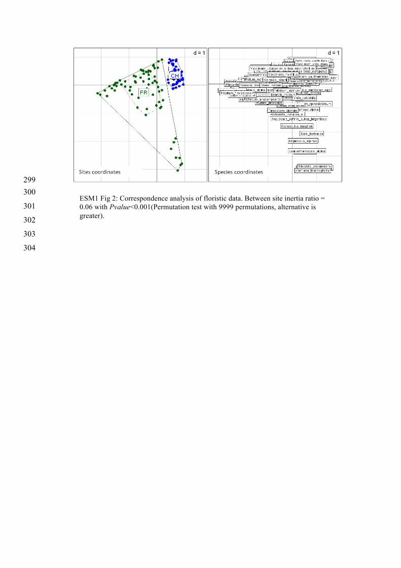
ESM1 Fig 2: Correspondence analysis of floristic data. Between site inertia ratio = 0.06 with Pvalue<0.001(Permutation test with 9999 permutations, alternative is greater).

305

CHFR

Festuca violacea aggrCarex sempervirens

Poa alpinaCerastium arvense sl

Geum montanumAnthoxanthum odoratum aggr

Pulsatilla alpina slMyosotis alpestris

Potentilla aureaTrifolium alpinumGentiana acaulis

Geranium sylvaticumPolygonum viviparumMeum athamanticum

Plantago alpinaCentaurea unifloraFestuca paniculata

Lotus alpinusPotentilla grandiflora

Veronica allioniiAlchemilla xanthochlora aggr

Alopecurus alpinusArnica montana

Rumex nebroidesLeontodon helveticusLeontodon hispidus sl

Pedicularis rostratospicataSenecio doronicum

Campanula scheuchzeriCarlina acaulis subsp caulescens

Luzula nutansViola calcarata

Luzula luteaHieracium villosum

Sempervivum montanumAnthyllis vulneraria sl

Phleum rhaeticumGentiana punctata

Nardus strictaPachypleurum mutellinoides

Phyteuma micheliiRanunculus kuepferiVaccinium myrtillus

Galium lucidumHelianthemum grandiflorum

Phyteuma orbicularePulmonaria angustifolia

Thymus praecox subsp polytrichusAchillea millefoliumAndrosace vitaliana

Carduus defloratus slEuphorbia cyparissiasHieracium armerioides

Homogyne alpinaKobresia myosuroides

Leucanthemopsis alpinaRanunculus montanus aggr

Trifolium pratense slVaccinium uliginosum subsp microphyllum

Laserpitium halleriAntennaria carpatica

Botrychium lunariaCarex foetida

Cirsium spinosissimumFestuca laevigata

Galium mollugo subsp erectumHelictotrichon sedenense

Myosotis arvensisOxytropis lapponicaRanunculus acris sl

Sempervivum arachnoideumSilene vulgaris sl

Taraxacum alpinumTrifolium repens sstr

Antennaria dioicaCarex curvula subsp rosae

Lilium martagonPedicularis tuberosa

Rhinanthus alectorolophusSaxifraga paniculata

Sesleria caeruleaTrifolium montanum

Achillea nanaBiscutella laevigataFestuca nigrescensFestuca rubra aggr

Sibbaldia procumbensSilene acaulisSilene nutansTrifolium thalii

Alchemilla pentaphylleaAlchemilla splendens

Aster alpinusDeschampsia flexuosa

Dryas octopetalaGentiana brachyphylla

Gentiana luteaLaserpitium latifolium

Minuartia sedoidesMinuartia verna

Nigritella cornelianaSalix herbacea

Sedum anacampserosSempervivum tectorum

Alchemilla coriacea slAndrosace adfinis subsp brigantiaca

Bartsia alpinaEmpetrum nigrum subsp hermaphroditum

Erigeron uniflorusGentianella campestris

Hieracium peleterianumLotus corniculatus aggr

Narcissus poeticusScutellaria alpinaSenecio incanusStachys pradica

Thesium alpinumTrifolium alpestre

Trisetum flavescens

frequency

0.0 0.2 0.4 0.6

Campanula scheuchzeriHomogyne alpina

Potentilla aureaLigusticum mutellina

Ranunculus montanus aggrPolygonum viviparum

Poa alpinaAlchemilla xanthochlora aggr

Leontodon hispidus slPlantago alpina

Carex sempervirensGalium anisophyllon

Soldanella alpinaAnthoxanthum odoratum aggr

Lotus corniculatus aggrNardus stricta

Trifolium pratense slPhleum rhaeticum

Anthyllis vulneraria slAgrostis capillarisEuphrasia minima

Crepis aureaFestuca rubra aggr

Sesleria caeruleaFestuca violacea aggr

Trifolium thaliiAster bellidiastrum

Plantago atrata sstrAgrostis rupestris

Alchemilla conjuncta aggrTrifolium repens sstr

Festuca quadrifloraGeum montanum

Helictotrichon versicolorPhyteuma orbiculare

Salix retusaScabiosa lucida

Dryas octopetalaGentiana campestris sstr

Leontodon helveticusBartsia alpina

Gentiana purpureaLuzula multiflora

Trollius europaeusAndrosace chamaejasme

Arnica montanaDeschampsia cespitosa

Gentiana acaulisPolygala alpestrisPotentilla crantzii

Vaccinium gaultherioidesHieracium lactucellaVaccinium myrtillusCarex ornithopoda

Carlina acaulis subsp caulescensHelianthemum nummularium sl

Luzula alpinopilosaPedicularis verticillata

Prunella vulgarisTaraxacum officinale aggr

Vaccinium vitis.idaeaViola calcarata

Alchemilla glabra aggrAposeris foetida

Campanula barbataCerastium fontanum sl

Gentiana vernaLeucanthemum vulgare aggr

Ranunculus acris slSalix herbacea

Trifolium badiumCrocus albiflorus

Thymus praecox subsp polytrichusAlchemilla vulgaris aggrCirsium spinosissimumLoiseleuria procumbens

Myosotis alpestrisThesium alpinum

frequency

0.0 0.2 0.4 0.6 0.8

ESM1 Fig 3: Species rank-frequency curves for the French (FR) and Swiss (CH) sites.

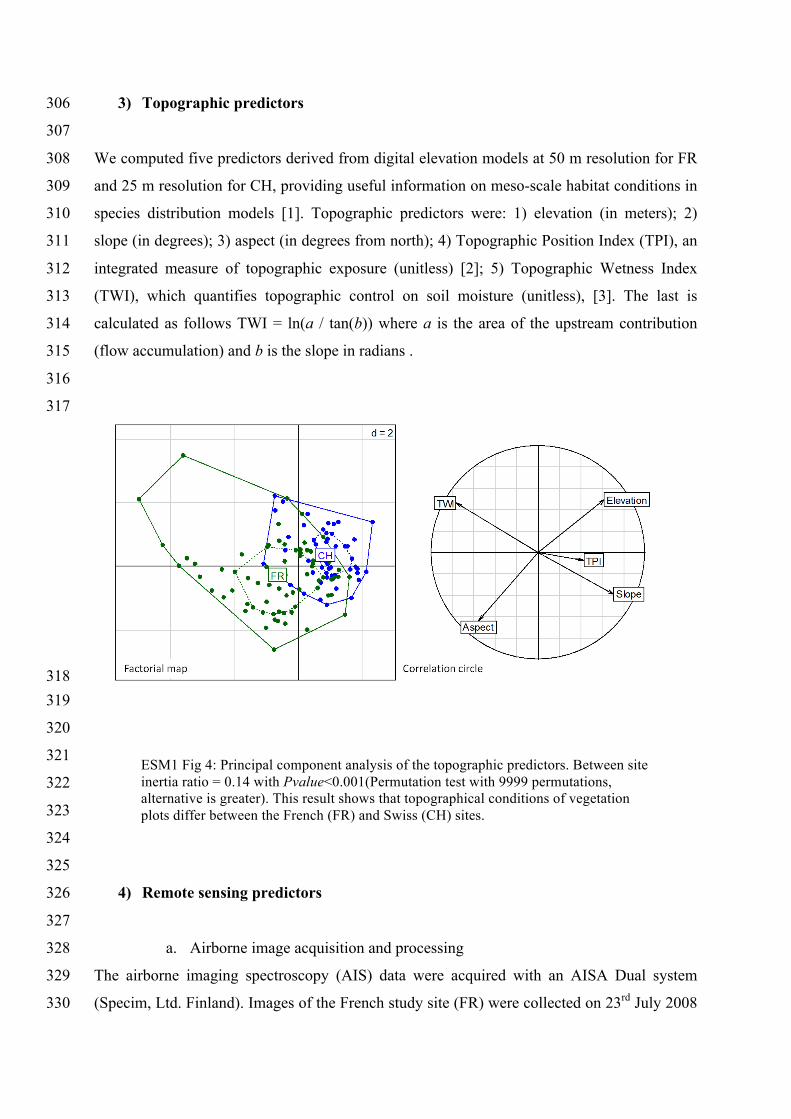
3) Topographic predictors 306

307

We computed five predictors derived from digital elevation models at 50 m resolution for FR 308

and 25 m resolution for CH, providing useful information on meso-scale habitat conditions in 309

species distribution models [1]. Topographic predictors were: 1) elevation (in meters); 2) 310

slope (in degrees); 3) aspect (in degrees from north); 4) Topographic Position Index (TPI), an 311

integrated measure of topographic exposure (unitless) [2]; 5) Topographic Wetness Index 312

(TWI), which quantifies topographic control on soil moisture (unitless), [3]. The last is 313

calculated as follows TWI = ln(a / tan(b)) where a is the area of the upstream contribution 314

(flow accumulation) and b is the slope in radians . 315

316

317

318 319

320

321

322

323

324

325

4) Remote sensing predictors 326

327

a. Airborne image acquisition and processing 328

The airborne imaging spectroscopy (AIS) data were acquired with an AISA Dual system 329

(Specim, Ltd. Finland). Images of the French study site (FR) were collected on 23rd July 2008 330

ESM1 Fig 4: Principal component analysis of the topographic predictors. Between site inertia ratio = 0.14 with Pvalue<0.001(Permutation test with 9999 permutations, alternative is greater). This result shows that topographical conditions of vegetation plots differ between the French (FR) and Swiss (CH) sites.

and for the Swiss study site (CH) on 24th July 2008 under clear sky and sunny conditions. 331

Images were acquired in a high spectral and spatial resolution mode, which resulted in a 332

spectral image data cube with 359 narrow spectral bands between 400 and 2450 nm and the 333

ground pixel size of 0.8 m. 334

335

The basic processing of AISA Dual images comprised of radiometric, geometric, and 336

atmospheric correction. The radiometric correction that converted image digital numbers into 337

radiance values [W.m-2.sr-1.µm-1] was performed in the CaliGeo software (CaliGeo v.4.6.4 - 338

AISA processing toolbox, Specim, 2007) using the factory delivered radiometric calibration 339

coefficients. Images were geometrically corrected using the onboard navigation data from the 340

Inertial Navigation System and a local digital elevation model (spatial resolution of 2.5 m for 341

FR and 1 m for CH site). Images were further orthorectified into the Universal Transverse 342

Mercator (UTM, Zone 32N) map projection. An accuracy of the geometric correction was 343

evaluated by calculating an average root mean square error (RMSE) between distinct image 344

displayed and ground measured control points. Assessment resulted into an average RMSE of 345

about 2.04 m for the French site and about 1.25 m for the Swiss site. Atmospheric corrections 346

were combined with vicarious radiometric calibrations in the ATCOR-4 software [4]. To 347

eliminate random noise, spectra of the atmospherically corrected images were smoothed by a 348

moving average filter with the window size of 7 bands. Accuracy of the atmospheric 349

corrections was evaluated by comparing image surface reflectance with a set of ground 350

measured reference spectra. An average reflectance RMSE between the image and the ground 351

target spectra was equal to 2.1% for the French and 1.6% for the Swiss site. As the final step 352

of the image processing we applied a fully constrained linear spectral unmixing algorithm [5] 353

to identify pixels with high vegetation fraction. Only pixels with vegetation fraction higher 354

than 75% were included into further analysis of species distribution modelling. 355

356

We paired the AISA image data with the georeferenced plots, where floristic species 357

composition was investigated in-situ. Their geographical locations were superimposed over 358

the AISA images and the reflectance function of each a research plot was averaged. Plots with 359

high proportion of non-vegetated pixels (i.e. pixels with vegetation fraction lower than 75% 360

due to the occurrence of stones or bare soil patches) were excluded. After this selection, we 361

retained 70 plots at the French site and 53 plots at the Swiss site. Two types of remote sensing 362

predictors were tested for the species distribution modelling: i) reflectance intensity of 75 363

noise-free bands and ii) four vegetation indices (summarized in Table 2). 364

365

b. Removal of spectral bands with low signal quality 366

Only 75 spectral bands out of 359 were included in the species distribution analysis. We 367

removed bands with poor signal quality due to the low radiometric sensitivity at the edges of 368

both sensor spectral ranges (401-444, 876-1140 and around 2450 nm), bands strongly 369

influenced by atmospheric water vapor absorption (i.e., 1334-1485 and 1786-1968 nm) and 370

adjacent bands of near infrared wavelengths between 752 and 771 nm, which are highly 371

correlated and contain redundant spectral information. 372

373 374

0 20 40 60

020

4060

Bands ID

Ban

ds ID

Wav

elen

gth

(nm

)

010

0020

00

Wavelength (nm)

0 1000 2000

A)  FR

A)  CH

0 20 40 60

020

4060

Bands ID

Ban

ds ID

Wav

elen

gth

(nm

)

010

0020

00

Wavelength (nm)

0 1000 2000

-0.5 0.0 0.5 1.0 1.5

0.0

0.2

0.4

0.6

0.8

1.0

-0.5

0.0

0.5

1.0

r

ESM1 Fig 5: Between reflectance bands correlation patterns for the French (FR) and Swiss (CH) sites. Although band selection (75 out of 359) led to the removal of highly correlated adjacent bands, many non-adjacent bands were strongly correlated. This justifies the use of unbiased conditional random forest in case of multicolinearity.

375 376

377

378

379

380

c. Calculation of vegetation indices and the between site PCA 381

382

Four vegetation optical indices, defined in Table 2, were selected as remote sensing indicators 383

of the vegetation biochemical and biophysical properties. Two indices are highly sensitive to 384

leaf chlorophyll content, but insensitive to the variations in amount of green biomass 385

(TCARI/OSAVI and ANCB650-720). MTVI2 index was chosen as an indicator of green leaf 386

area index, while suppressing negative confounding influence of leaf chlorophyll content. 387

Finally, SIWSI index is sensitive to plant water content. The variability of the selected optical 388

indices is expected to be species composition specific in accordance with the species-specific 389

changes of the related biochemical and biophysical characteristics. These four indices can 390

thus potentially discriminate key properties of the species, justifying their use for species 391

distribution modeling. 392

393

ESM1 Fig 6: Principal component analysis of the 75 reflectance bands. Between site inertia ratio = 0.06 with Pvalue<0.001(Permutation test with 9999 permutations, alternative is greater). This result shows that reflectance pattern of vegetation plots differed between the French (FR) and Swiss (CH) sites.

394

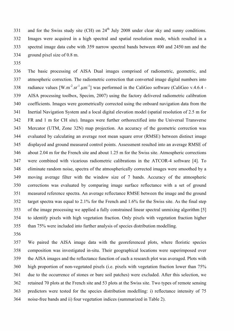
EMS 1 Table 2: Vegetation indices tested for species distribution modeling 395 396 Vegetation index Equation Reference Transformed Chlorophyll Absorbtion Reflectance Index / Optimized Soil-Adjusted Vegetation Index (TCARI/OSAVI)

TCARI = 3[R!"" − R!"# − 0.2 R!"" −R!!" (R!"" R!"#)]

OSAVI =1.16(𝑅!"" − 𝑅!"#)𝑅!"" + 𝑅!"# + 0.16

Haboudane et al, (2002) [5]

Area under curve Normalized to the Continuum-removed Band depth (ANCB650-720)

AUC!"#!!"#CBD!"#

where AUC650-720 is area under continuum removed reflectance between 650-720 nm and CBD670 is continuum removed band depth at 670 nm

Malenovský et al. (2013) [6]

Modified Triangular Vegetation Index (MTVI2)

1.5[1.2 R!"" − R!!" − 2.5(R!"# − R!!")]

(2R!"" + 1)! − 6R!"" − 5 R!"# − 0.5

Haboudane et al. (2004) [7]

Shortwave Infrared Water Stress Index (SIWSI)

R!"!.! − R!"#$R!"!.! + R!"#$

Cheng et al. (2006) [8]

397

398

399 400

401

402

403

d. Correlation of AIS-data with topographic predictors 404

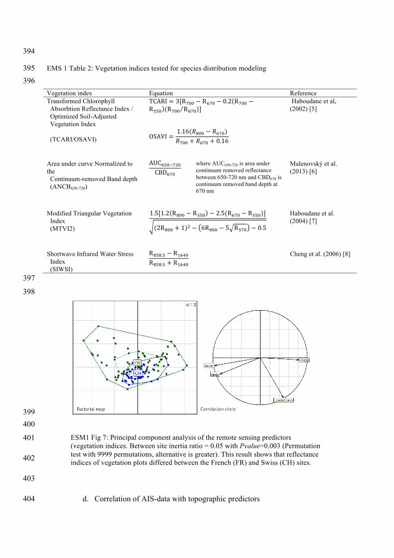
ESM1 Fig 7: Principal component analysis of the remote sensing predictors (vegetation indices. Between site inertia ratio = 0.05 with Pvalue=0.003 (Permutation test with 9999 permutations, alternative is greater). This result shows that reflectance indices of vegetation plots differed between the French (FR) and Swiss (CH) sites.

AIS and topographical data were weakly correlated (max absolute values for Pearson 405

correlations amounted to 0.40-0.55 between elevation and bands in the range of 2000 and 406

2500 nm, while most of absolute values for Pearson correlation coefficients are between 0 and 407

0.3). Absence of strong correlation allows for mixing both types of data in species distribution 408

models, as topographic- (indicating meso-scale habitat suitability of the species) and fine-409

scale AIS-data may represent complementary information. 410

5) Selection of spectral bands for building final species distribution models 411

Based on the analysis performed to quantify the importance of each of the 75 spectral bands, 412

we built final species distribution models according to the following variable selection 413

procedure: 414

1. Rank bands in decreasing order of importance 415

2. While not all bands have been considered, select the first ranked band (with the 416

highest relative importance) and remove all bands showing correlation >0.7 with the 417

previously selected band. 418

This procedure was performed with random forest (RF) using conditional inference trees as 419

base learners and was implemented with the party library [9] for R [10]. Variable importance 420

is measured as the mean decrease in accuracy of model predictions after permuting the 421

predictor variables. 422

References 423

1. Pradervand, J.-N., Dubuis, A., Pellissier, L., Guisan, A. & Randin, C. 2013 Very high 424 resolution environmental predictors in species distribution models: Moving beyond 425 topography? Prog. Phys. Geogr. 38, 79–96. (doi:10.1177/0309133313512667) 426

2. Zimmermann, N. E., Edwards, T. C., Moisen, G. G., Frescino, T. S. & Blackard, J. A. 427 2007 Remote sensing-based predictors improve distribution models of rare, early 428 successional and broadleaf tree species in Utah. J. Appl. Ecol. 44, 1057–1067. 429 (doi:10.1111/j.1365-2664.2007.01348.x) 430

3. Beven, K. J. & Kirkby, M. J. 1979 A physically based, variable contributing area 431 model of basin hydrology. Bull. Int. Assoc. Sci. Hydrol. 24, 43–69. 432

4. Richter, R. & Schlapfer, D. 2002 Geo-atmospheric processing of airborne imaging 433 spectrometry data. Part 2: Atmospheric/topographic correction. Int. J. Remote Sens. 23, 434 2631–2649. (doi:10.1080/01431160110115834) 435

5. Haboudane, D., Miller, J. R., Tremblay, N., Zarco-Tejada, P. J. & Dextraze, L. 2002 436 Integrated narrow-band vegetation indices for prediction of crop chlorophyll content 437 for application to precision agriculture. Remote Sens. Environ. 81, 416–426. 438 (doi:10.1016/S0034-4257(02)00018-4) 439

6. Malenovský, Z., Homolová, L., Zurita-Milla, R., Lukeš, P., Kaplan, V., Hanuš, J., 440 Gastellu-Etchegorry, J.-P. & Schaepman, M. E. 2013 Retrieval of spruce leaf 441 chlorophyll content from airborne image data using continuum removal and radiative 442 transfer. Remote Sens. Environ. 131, 85–102. (doi:10.1016/j.rse.2012.12.015) 443

7. Haboudane, D., Millera, J. R., Pattey, E., Zarco-Tejada, P. J. & Strachan, I. B. 2004 444 Hyperspectral vegetation indices and novel algorithms for predicting green LAI of crop 445 canopies: Modeling and validation in the context of precision agriculture. Remote Sens. 446 Environ. 90, 337–352. (doi:10.1016/j.rse.2003.12.013) 447

8. Cheng, Y.-B., Zarco-Tejada, P. J., Riaño, D., Rueda, C. A. & Ustin, S. L. 2006 448 Estimating vegetation water content with hyperspectral data for different canopy 449 scenarios: Relationships between AVIRIS and MODIS indexes. Remote Sens. Environ. 450 105, 354–366. (doi:10.1016/j.rse.2006.07.005) 451

9. Strobl, C., Hothorn, T. & Zeileis, A. 2009 Party on! A New, Conditional Variable 452 Importance Measure for Random Forests Available in the party Package. , 1–4. 453

10. R Core Team 2013 R: A Language and Environment for Statistical Computing. 454

455

456

Electronic Supplementary Material 2: 457

Complementary results. 458

459

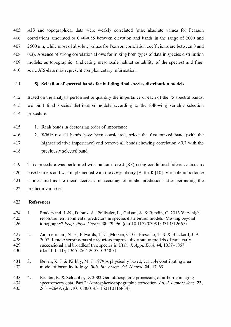
1) Relative importance of reflectance intensity in spectral bands for predicting the 460

distribution of species recorded only in one of the two sites or recorded in both 461

sites. 462

463

464 465

466

467

468

500

1000

1500

2000

2500

0.00

0.02

0.04

0.06

0.08

Species only in FR

Wavelength (nm)

Rel

ativ

e V

aria

ble

Impo

rtanc

e

500

1000

1500

2000

2500

0.00

0.02

0.04

0.06

Species only in CH

Wavelength (nm)

Rel

ativ

e V

aria

ble

Impo

rtanc

e

500

1000

1500

2000

2500

0.00

0.01

0.02

0.03

0.04

0.05

0.06

0.07

Common species in FR

Wavelength (nm)

Rel

ativ

e V

aria

ble

Impo

rtanc

e

500

1000

1500

2000

2500

0.00

0.01

0.02

0.03

0.04

0.05

Common species in CH

Wavelength (nm)

Rel

ativ

e V

aria

ble

Impo

rtanc

e

ESM2 Fig 1: Relative importance of reflectance intensity in spectral bands for predicting the distribution of species recorded only in the French site (FR), only in the Swiss site (CH), recorded in both sites but modeled in the French site and recorded in both sites but modeled in the Swiss site. Gray areas represent bands used for the calculation of the vegetation indices.

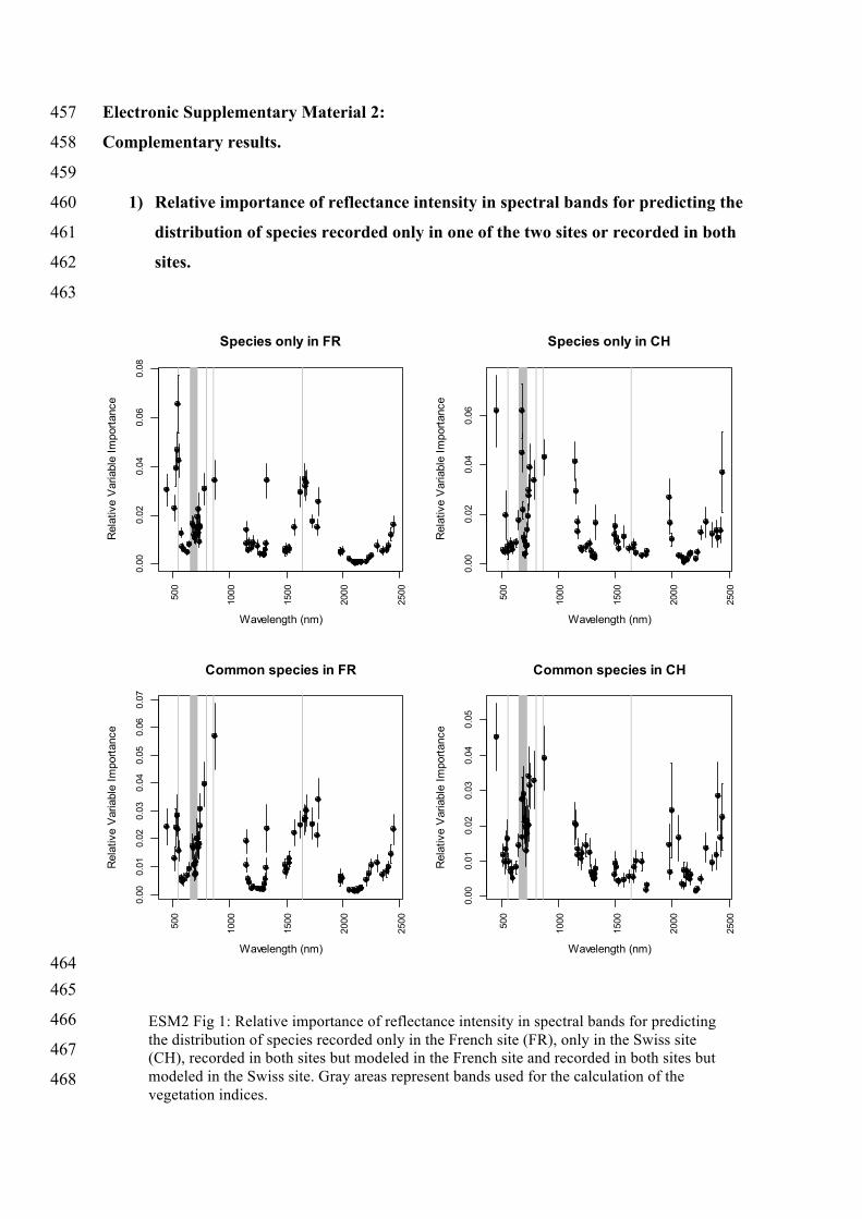
2) Variable importance of vegetation indices for the French site (FR) and the Swiss 469

site (CH). 470

471 472

473

474

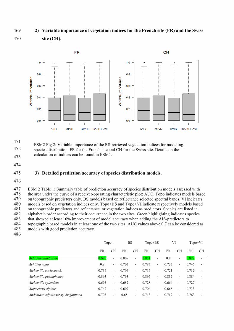
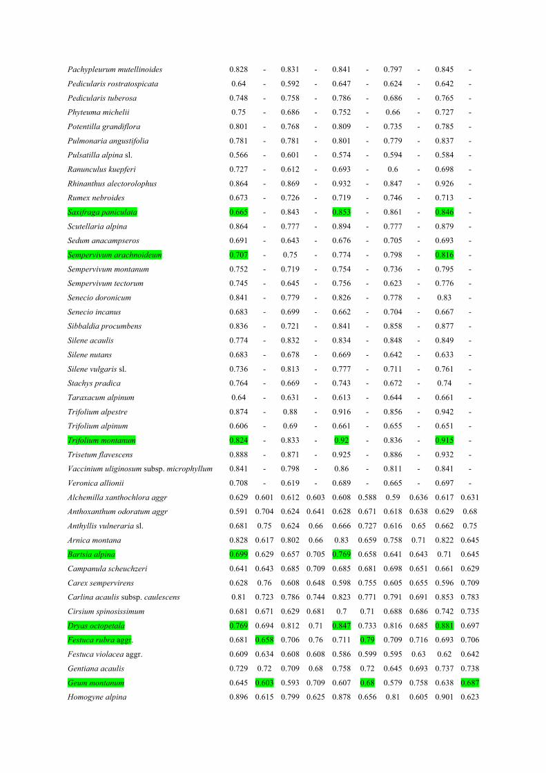
3) Detailed prediction accuracy of species distribution models. 475

476

ESM 2 Table 1: Summary table of prediction accuracy of species distribution models assessed with 477 the area under the curve of a receiver-operating characteristic plot: AUC. Topo indicates models based 478 on topographic predictors only, BS models based on reflectance selected spectral bands. VI indicates 479 models based on vegetation indices only. Topo+BS and Topo+VI indicate respectively models based 480 on topographic predictors and reflectance or vegetation indices as predictors. Species are listed in 481 alphabetic order according to their occurrence in the two sites. Green highlighting indicates species 482 that showed at least 10% improvement of model accuracy when adding the AIS-predictors to 483 topographic based models in at least one of the two sites. AUC values above 0.7 can be considered as 484 models with good prediction accuracy. 485 486

Topo BS Topo+BS VI Topo+VI

FR CH FR CH FR CH FR CH FR CH

Achillea millefolium 0.686 - 0.807 - 0.811 - 0.8 - 0.827 -

Achillea nana 0.8 - 0.703 - 0.783 - 0.737 - 0.746 -

Alchemilla coriacea sl. 0.735 - 0.707 - 0.717 - 0.721 - 0.732 -

Alchemilla pentaphyllea 0.893 - 0.763 - 0.897 - 0.817 - 0.884 -

Alchemilla splendens 0.695 - 0.682 - 0.728 - 0.664 - 0.727 -

Alopecurus alpinus 0.742 - 0.607 - 0.704 - 0.668 - 0.733 -

Androsace adfinis subsp. brigantiaca 0.703 - 0.65 - 0.713 - 0.719 - 0.763 -

ESM2 Fig 2: Variable importance of the RS-retrieved vegetation indices for modeling species distribution. FR for the French site and CH for the Swiss site. Details on the calculation of indices can be found in ESM1.

Androsace vitaliana 0.666 - 0.785 - 0.786 - 0.786 - 0.76 -

Antennaria carpatica 0.776 - 0.757 - 0.823 - 0.743 - 0.787 -

Antennaria dioica 0.783 - 0.675 - 0.783 - 0.639 - 0.737 -

Aster alpinus 0.703 - 0.689 - 0.664 - 0.662 - 0.711 -

Biscutella laevigata 0.795 - 0.631 - 0.722 - 0.627 - 0.755 -

Botrychium lunaria 0.681 - 0.704 - 0.679 - 0.722 - 0.711 -

Carduus defloratus sl. 0.852 - 0.796 - 0.817 - 0.751 - 0.836 -

Carex curvula subsp. rosae 0.789 - 0.803 - 0.827 - 0.82 - 0.764 -

Carex foetida 0.78 - 0.655 - 0.721 - 0.67 - 0.763 -

Centaurea uniflora 0.781 - 0.8 - 0.864 - 0.779 - 0.837 -

Cerastium arvense sl. 0.677 - 0.581 - 0.663 - 0.592 - 0.689 -

Deschampsia flexuosa 0.658 - 0.653 - 0.597 - 0.729 - 0.657 -

Empetrum nigrum subsp. hermaphroditum 0.943 - 0.843 - 0.933 - 0.897 - 0.931 -

Erigeron uniflorus 0.656 - 0.664 - 0.66 - 0.672 - 0.673 -

Euphorbia cyparissias 0.832 - 0.785 - 0.842 - 0.755 - 0.852 -

Festuca laevigata 0.846 - 0.681 - 0.859 - 0.702 - 0.87 -

Festuca nigrescens 0.607 - 0.705 - 0.658 - 0.686 - 0.62 -

Festuca paniculata 0.741 - 0.746 - 0.782 - 0.783 - 0.839 -

Galium lucidum 0.776 - 0.66 - 0.746 - 0.613 - 0.765 -

Galium mollugo subsp. erectum 0.87 - 0.756 - 0.848 - 0.73 - 0.874 -

Gentiana brachyphylla 0.882 - 0.664 - 0.859 - 0.736 - 0.903 -

Gentiana lutea 0.949 - 0.801 - 0.942 - 0.737 - 0.943 -

Gentiana punctata 0.709 - 0.706 - 0.708 - 0.692 - 0.71 -

Gentianella campestris 0.719 - 0.656 - 0.676 - 0.686 - 0.708 -

Geranium sylvaticum 0.775 - 0.796 - 0.801 - 0.82 - 0.821 -

Helianthemum grandiflorum 0.775 - 0.642 - 0.74 - 0.62 - 0.752 -

Helictotrichon sedenense 0.64 - 0.858 - 0.839 - 0.849 - 0.837 -

Hieracium armerioides 0.633 - 0.692 - 0.666 - 0.72 - 0.645 -

Hieracium peleterianum 0.645 - 0.692 - 0.635 - 0.673 - 0.648 -

Hieracium villosum 0.616 - 0.608 - 0.645 - 0.613 - 0.597 -

Kobresia myosuroides 0.68 - 0.695 - 0.732 - 0.738 - 0.73 -

Laserpitium halleri 0.73 - 0.803 - 0.771 - 0.718 - 0.701 -

Laserpitium latifolium 0.864 - 0.852 - 0.908 - 0.82 - 0.87 -

Leucanthemopsis alpina 0.734 - 0.822 - 0.861 - 0.829 - 0.858 -

Lilium martagon 0.819 - 0.806 - 0.789 - 0.783 - 0.839 -

Lotus alpinus 0.626 - 0.624 - 0.628 - 0.602 - 0.615 -

Luzula lutea 0.725 - 0.762 - 0.762 - 0.753 - 0.754 -

Luzula nutans 0.623 - 0.657 - 0.669 - 0.631 - 0.633 -

Meum athamanticum 0.829 - 0.919 - 0.931 - 0.881 - 0.888 -

Minuartia sedoides 0.783 - 0.77 - 0.806 - 0.779 - 0.767 -

Minuartia verna 0.753 - 0.824 - 0.817 - 0.821 - 0.896 -

Myosotis arvensis 0.85 - 0.859 - 0.876 - 0.822 - 0.847 -

Narcissus poeticus 0.935 - 0.875 - 0.951 - 0.886 - 0.942 -

Nigritella corneliana 0.615 - 0.592 - 0.622 - 0.631 - 0.621 -

Oxytropis lapponica 0.645 - 0.733 - 0.662 - 0.632 - 0.641 -

Pachypleurum mutellinoides 0.828 - 0.831 - 0.841 - 0.797 - 0.845 -

Pedicularis rostratospicata 0.64 - 0.592 - 0.647 - 0.624 - 0.642 -

Pedicularis tuberosa 0.748 - 0.758 - 0.786 - 0.686 - 0.765 -

Phyteuma michelii 0.75 - 0.686 - 0.752 - 0.66 - 0.727 -

Potentilla grandiflora 0.801 - 0.768 - 0.809 - 0.735 - 0.785 -

Pulmonaria angustifolia 0.781 - 0.781 - 0.801 - 0.779 - 0.837 -

Pulsatilla alpina sl. 0.566 - 0.601 - 0.574 - 0.594 - 0.584 -

Ranunculus kuepferi 0.727 - 0.612 - 0.693 - 0.6 - 0.698 -

Rhinanthus alectorolophus 0.864 - 0.869 - 0.932 - 0.847 - 0.926 -

Rumex nebroides 0.673 - 0.726 - 0.719 - 0.746 - 0.713 -

Saxifraga paniculata 0.665 - 0.843 - 0.853 - 0.861 - 0.846 -

Scutellaria alpina 0.864 - 0.777 - 0.894 - 0.777 - 0.879 -

Sedum anacampseros 0.691 - 0.643 - 0.676 - 0.705 - 0.693 -

Sempervivum arachnoideum 0.707 - 0.75 - 0.774 - 0.798 - 0.816 -

Sempervivum montanum 0.752 - 0.719 - 0.754 - 0.736 - 0.795 -

Sempervivum tectorum 0.745 - 0.645 - 0.756 - 0.623 - 0.776 -

Senecio doronicum 0.841 - 0.779 - 0.826 - 0.778 - 0.83 -

Senecio incanus 0.683 - 0.699 - 0.662 - 0.704 - 0.667 -

Sibbaldia procumbens 0.836 - 0.721 - 0.841 - 0.858 - 0.877 -

Silene acaulis 0.774 - 0.832 - 0.834 - 0.848 - 0.849 -

Silene nutans 0.683 - 0.678 - 0.669 - 0.642 - 0.633 -

Silene vulgaris sl. 0.736 - 0.813 - 0.777 - 0.711 - 0.761 -

Stachys pradica 0.764 - 0.669 - 0.743 - 0.672 - 0.74 -

Taraxacum alpinum 0.64 - 0.631 - 0.613 - 0.644 - 0.661 -

Trifolium alpestre 0.874 - 0.88 - 0.916 - 0.856 - 0.942 -

Trifolium alpinum 0.606 - 0.69 - 0.661 - 0.655 - 0.651 -

Trifolium montanum 0.824 - 0.833 - 0.92 - 0.836 - 0.915 -

Trisetum flavescens 0.888 - 0.871 - 0.925 - 0.886 - 0.932 -

Vaccinium uliginosum subsp. microphyllum 0.841 - 0.798 - 0.86 - 0.811 - 0.841 -

Veronica allionii 0.708 - 0.619 - 0.689 - 0.665 - 0.697 -

Alchemilla xanthochlora aggr 0.629 0.601 0.612 0.603 0.608 0.588 0.59 0.636 0.617 0.631

Anthoxanthum odoratum aggr 0.591 0.704 0.624 0.641 0.628 0.671 0.618 0.638 0.629 0.68

Anthyllis vulneraria sl. 0.681 0.75 0.624 0.66 0.666 0.727 0.616 0.65 0.662 0.75

Arnica montana 0.828 0.617 0.802 0.66 0.83 0.659 0.758 0.71 0.822 0.645

Bartsia alpina 0.699 0.629 0.657 0.705 0.769 0.658 0.641 0.643 0.71 0.645

Campanula scheuchzeri 0.641 0.643 0.685 0.709 0.685 0.681 0.698 0.651 0.661 0.629

Carex sempervirens 0.628 0.76 0.608 0.648 0.598 0.755 0.605 0.655 0.596 0.709

Carlina acaulis subsp. caulescens 0.81 0.723 0.786 0.744 0.823 0.771 0.791 0.691 0.853 0.783

Cirsium spinosissimum 0.681 0.671 0.629 0.681 0.7 0.71 0.688 0.686 0.742 0.735

Dryas octopetala 0.769 0.694 0.812 0.71 0.847 0.733 0.816 0.685 0.881 0.697

Festuca rubra aggr. 0.681 0.658 0.706 0.76 0.711 0.79 0.709 0.716 0.693 0.706

Festuca violacea aggr. 0.609 0.634 0.608 0.608 0.586 0.599 0.595 0.63 0.62 0.642

Gentiana acaulis 0.729 0.72 0.709 0.68 0.758 0.72 0.645 0.693 0.737 0.738

Geum montanum 0.645 0.603 0.593 0.709 0.607 0.68 0.579 0.758 0.638 0.687

Homogyne alpina 0.896 0.615 0.799 0.625 0.878 0.656 0.81 0.605 0.901 0.623

Leontodon helveticus 0.59 0.677 0.666 0.746 0.642 0.772 0.663 0.71 0.615 0.715

Leontodon hispidus sl. 0.802 0.659 0.8 0.645 0.818 0.699 0.735 0.61 0.859 0.665

Lotus corniculatus aggr. 0.862 0.616 0.71 0.608 0.859 0.608 0.713 0.601 0.901 0.61

Myosotis alpestris 0.672 0.729 0.713 0.639 0.735 0.664 0.735 0.608 0.753 0.693

Nardus stricta 0.654 0.613 0.624 0.659 0.644 0.655 0.625 0.667 0.641 0.647

Phleum rhaeticum 0.68 0.683 0.75 0.576 0.724 0.682 0.718 0.653 0.692 0.701

Phyteuma orbiculare 0.631 0.66 0.614 0.62 0.603 0.626 0.625 0.614 0.578 0.638

Plantago alpina 0.619 0.618 0.621 0.621 0.619 0.631 0.671 0.59 0.635 0.588

Poa alpina 0.788 0.647 0.619 0.633 0.795 0.655 0.625 0.627 0.764 0.64

Polygonum viviparum 0.718 0.652 0.653 0.685 0.698 0.691 0.722 0.615 0.743 0.655

Potentilla aurea 0.625 0.612 0.669 0.746 0.659 0.75 0.571 0.745 0.596 0.725

Ranunculus acris sl. 0.664 0.68 0.748 0.665 0.748 0.662 0.803 0.731 0.799 0.681

Ranunculus montanus aggr. 0.684 0.599 0.745 0.652 0.744 0.642 0.727 0.714 0.781 0.677

Salix herbacea 0.741 0.655 0.781 0.686 0.818 0.639 0.791 0.62 0.811 0.669

Sesleria caerulea 0.666 0.655 0.752 0.705 0.737 0.718 0.797 0.671 0.783 0.713

Thesium alpinum 0.71 0.66 0.793 0.781 0.791 0.747 0.84 0.718 0.788 0.678

Thymus praecox subsp. polytrichus 0.771 0.649 0.694 0.748 0.803 0.717 0.655 0.757 0.756 0.649

Trifolium pratense sl. 0.759 0.592 0.66 0.75 0.72 0.731 0.67 0.697 0.732 0.678

Trifolium repens sstr. 0.651 0.747 0.609 0.691 0.611 0.746 0.639 0.786 0.673 0.749

Trifolium thalii 0.623 0.606 0.66 0.612 0.612 0.607 0.635 0.606 0.634 0.616

Vaccinium myrtillus 0.882 0.647 0.801 0.671 0.858 0.623 0.779 0.643 0.848 0.659

Viola calcarata 0.627 0.68 0.613 0.614 0.624 0.616 0.624 0.737 0.622 0.628

Agrostis capillaris - 0.66 - 0.771 - 0.774 - 0.793 - 0.852

Agrostis rupestris - 0.685 - 0.762 - 0.721 - 0.598 - 0.666

Alchemilla conjuncta aggr. - 0.599 - 0.684 - 0.697 - 0.669 - 0.629

Alchemilla glabra aggr. - 0.671 - 0.736 - 0.705 - 0.619 - 0.66

Alchemilla vulgaris aggr. - 0.74 - 0.634 - 0.65 - 0.655 - 0.674

Androsace chamaejasme - 0.658 - 0.602 - 0.643 - 0.61 - 0.646

Aposeris foetida - 0.788 - 0.714 - 0.818 - 0.692 - 0.838

Aster bellidiastrum - 0.705 - 0.646 - 0.741 - 0.657 - 0.758

Campanula barbata - 0.703 - 0.789 - 0.745 - 0.787 - 0.72

Carex ornithopoda - 0.707 - 0.638 - 0.68 - 0.612 - 0.677

Cerastium fontanum sl. - 0.682 - 0.684 - 0.706 - 0.683 - 0.685

Crepis aurea - 0.634 - 0.716 - 0.639 - 0.636 - 0.597

Crocus albiflorus - 0.744 - 0.733 - 0.769 - 0.727 - 0.781

Deschampsia cespitosa - 0.683 - 0.715 - 0.726 - 0.773 - 0.754

Euphrasia minima - 0.585 - 0.66 - 0.624 - 0.6 - 0.606

Festuca quadriflora - 0.634 - 0.767 - 0.737 - 0.679 - 0.647

Galium anisophyllon - 0.767 - 0.609 - 0.753 - 0.713 - 0.771

Gentiana campestris sstr. - 0.705 - 0.597 - 0.665 - 0.65 - 0.673

Gentiana purpurea - 0.62 - 0.81 - 0.797 - 0.788 - 0.746

Gentiana verna - 0.682 - 0.681 - 0.663 - 0.674 - 0.646

Helianthemum nummularium sl. - 0.631 - 0.631 - 0.627 - 0.638 - 0.624

Helictotrichon versicolor - 0.627 - 0.607 - 0.615 - 0.597 - 0.605

Hieracium lactucella - 0.648 - 0.755 - 0.761 - 0.771 - 0.748

Leucanthemum vulgare aggr. - 0.864 - 0.756 - 0.888 - 0.707 - 0.911

Ligusticum mutellina - 0.624 - 0.677 - 0.671 - 0.741 - 0.698

Loiseleuria procumbens - 0.66 - 0.639 - 0.601 - 0.635 - 0.624

Luzula alpinopilosa - 0.671 - 0.69 - 0.681 - 0.711 - 0.688

Luzula multiflora - 0.715 - 0.582 - 0.643 - 0.608 - 0.684

Pedicularis verticillata - 0.682 - 0.657 - 0.693 - 0.627 - 0.681

Plantago atrata sstr. - 0.6 - 0.614 - 0.607 - 0.605 - 0.593

Polygala alpestris - 0.633 - 0.643 - 0.637 - 0.702 - 0.615

Potentilla crantzii - 0.639 - 0.67 - 0.635 - 0.657 - 0.625

Prunella vulgaris - 0.683 - 0.622 - 0.661 - 0.63 - 0.634

Salix retusa - 0.68 - 0.688 - 0.764 - 0.661 - 0.748

Scabiosa lucida - 0.647 - 0.678 - 0.727 - 0.607 - 0.633

Soldanella alpina - 0.642 - 0.717 - 0.717 - 0.683 - 0.677

Taraxacum officinale aggr. - 0.757 - 0.627 - 0.685 - 0.761 - 0.681

Trifolium badium - 0.689 - 0.696 - 0.666 - 0.695 - 0.66

Trollius europaeus - 0.667 - 0.812 - 0.8 - 0.715 - 0.75

Vaccinium gaultherioides - 0.633 - 0.648 - 0.641 - 0.624 - 0.647

Vaccinium vitis-idaea - 0.705 - 0.666 - 0.674 - 0.644 - 0.723

487

488

489

490 491

492

493

ESM2 Fig 3: Proportions of species distribution models for which accuracy was improved by 10% (dark green areas) or between 0 and 10% (light green areas) or was declined (gray areas) when adding the AIS-predictors to topographic based models. FR for the French site and CH for the Swiss site. BS indicates reflectance records in spectral bands as predictors and VI indicates vegetation indices as predictors. See ESM2 Table 1 for identity of the species that showed best model improvement.

494

Weak or no improvement of species distribution models, when including AIS-predictors, 495

suggests that the ecological information represented by AIS-data was redundant to already 496

included topography indicators. Increasing the dimensionality of the set of predictors without 497

additional informational content may flaw the fitted statistical relationships and ultimately 498

decrease model accuracy as we observed for many species at both sites. 499

500

4) The effect of species abundance patterns on the prediction accuracy of remote 501

sensing–based species distribution models. 502

503 504

505 ESM2 Fig 4: Relationships between four predictors of species abundance patterns and the accuracy of species distribution models based on the reflectance records in spectral bands (BS). White points for species from the French site (FR) and black points for species from the Swiss site (CH).

506

507

508 509

510 511 512 513 514

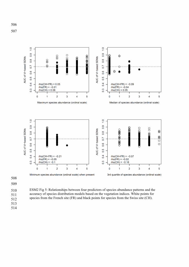
ESM2 Fig 5: Relationships between four predictors of species abundance patterns and the accuracy of species distribution models based on the vegetation indices. White points for species from the French site (FR) and black points for species from the Swiss site (CH).

5) Testing the phylogenetic and functional dependency of model features between 515 the species. 516 517

We implemented a similar procedure as for the test of phylogenetic signal of species traits, 518

except were considered the AUC values and AIS-predictor importance as traits and we sought 519

for both phylogenetic and functional signals. Specifically, we implemented two 520

complementary analyses following recommendations of Hardy and Pavoine 2012 [1]. In the 521

first, we computed a global Mantel test contrasting dissimilarity of species distribution models 522

(Euclidean distance between AUC values or AIS-variable importance) and phylogenetic or 523

functional dissimilarity between the species. The randomisation procedure consisted of 524

random reallocation of AUC values or variable importance between the species (999 525

permutations). In the second, we computed distograms where species model dissimilarities 526

(again as Euclidean distance between AUC values or AIS-variable importance) are plotted 527

against classes of phylogenetic or functional distance between the species. This indicates how 528

species models differ for functionally/phylogenetically closely related species and for 529

dissimilar species. 530

531

Phylogenic information for the French site was extracted from the complete phylogeny for the 532

Alpine flora at the genus level published in Thuiller et al. 2014 [2]. Finally, we randomly 533

resolved terminal polytomies by applying a birth-death (Yule) bifurcation process within each 534

genus [3]. Phylogenetic information for the Swiss site was extracted from the phylogeny for 535

the 231 most frequent species of the Western Swiss Alps of the Canton of Vaud (a 700 km² 536

region surrounding the Swiss site Anzeindaz). This phylogeny is based on DNA sequences 537

extracted from collected vegetal material and built by alignment of chloroplastic DNA 538

sequences (rbcl and matK) with GTR + gamma models of evolution under a Bayesian 539

inference framework. Details are available in Ndiribe et al. 2013 [4]. 540

All the species of the French site (i.e. 119) were included in phylogenetic tests while 69 541

species of the Swiss site (on 78) could be accounted for. 542

The phylogenetic distance between the species was quantified using the Abouheif proximity 543

measure for Mantel tests and the square-root of patristic distance for distograms [1]. 544

545

Traits information included morphological and physiological traits that are acknowledged to 546

indicate plant fitness, community dynamics and ecosystem processes. Some of them are also 547

recognized to be related to the reflectance pattern of vegetation stands [5,6]. We considered: 548

1) specific leaf area (SLA; m².kg-1), 2) leaf dry matter content (LDMC, mg.g-1), 3) vegetation 549

height (mm), 4) plant growth form discriminating species as graminoid, forb, legume or 550

shrub, 5) Leaf distribution along the stem discriminating species with leaves growing 551

regularly along the stem, rosette or tufted species and semi rosette species, and 6) branching, a 552

binary trait describing species ability to fill lateral space. SLA, LDMC and vegetation height 553

were measured for most species in the field within each of the two sites (89 out 119 for FR 554

and 71 out of 78 for CH). Leaf distribution, growth form, and branching were retrieved from 555

the LEDA database [7]. Since trait data covered continuous and categorical variables, the 556

functional dissimilarity between species was quantified using the Gower distance metric [8] 557

for both Mantel tests and distogram computation. 558

559

Tests for phylogenetic and functional dependency of the importance of AIS-variables 560

considered only the species that showed distribution models with fair to good prediction 561

accuracy (i.e. AUC > 0.7) in order to exclude spurious estimates of variable importance from 562

inaccurate models. This led to analyses with reduced list of species as follows: 563

564

Number of species included in the

analyses

FR CH

Phylogenetic

(119/119sp)

Functional

(89/119sp)

Phylogenetic

(69/78sp)

Functional

(71/78sp)

Reflectance in spectral bands 64 47 25 25

Vegetation indices 68 50 19 20

565

566 567 568 569 570 571

ESM2 Fig 6: Phylogenetic dependency of model accuracy (AUC: the area under the curve of a receiver-operating characteristic plot) between the species for the French site (FR). The x-axis represents the phylogenetic distance between the species and the y-axis differences in AUC. Topo indicates models based on topographic predictors only, BS models based on reflectance recorded in the spectral bands. VI indicates models based on vegetation indices only. Topo+BS and Topo+VI indicate respectively models based on topographic predictors and reflectance records in spectral bands or vegetation indices as predictors. Confidence intervals were computed with random re-allocation of AUC values between the species (9999 permutations)

572 573

574

ESM2 Fig 7: Phylogenetic dependency of model accuracy (AUC: the area under the curve of a receiver-operating characteristic plot) between the species for the Swiss site (CH). The x-axis represents the phylogenetic distance between the species and the y-axis differences in AUC. Topo indicates models based on topographic predictors only, BS models based on reflectance recorded in the spectral bands. VI indicates models based on vegetation indices only. Topo+BS and Topo+VI indicate respectively models based on topographic predictors and reflectance records in spectral bands or vegetation indices as predictors. Confidence intervals were computed with random re-allocation of AUC values between the species (9999 permutations)

575 576 577 578 579 580

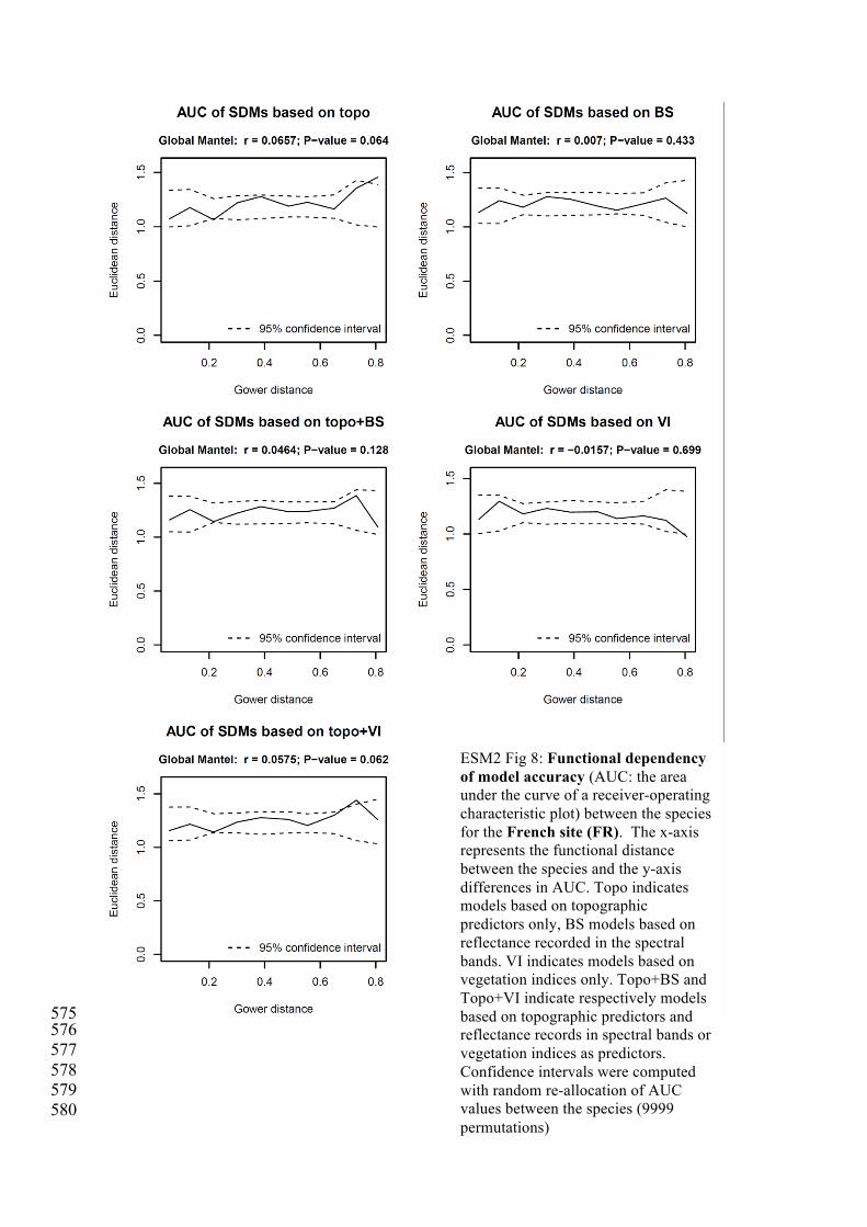
ESM2 Fig 8: Functional dependency of model accuracy (AUC: the area under the curve of a receiver-operating characteristic plot) between the species for the French site (FR). The x-axis represents the functional distance between the species and the y-axis differences in AUC. Topo indicates models based on topographic predictors only, BS models based on reflectance recorded in the spectral bands. VI indicates models based on vegetation indices only. Topo+BS and Topo+VI indicate respectively models based on topographic predictors and reflectance records in spectral bands or vegetation indices as predictors. Confidence intervals were computed with random re-allocation of AUC values between the species (9999 permutations)

581 582

ESM2 Fig 9: Functional dependency of model accuracy (AUC: the area under the curve of a receiver-operating characteristic plot) between the species for the Swiss site (CH). The x-axis represents the functional distance between the species and the y-axis differences in AUC. Topo indicates models based on topographic predictors only, BS models based on reflectance recorded in the spectral bands. VI indicates models based on vegetation indices only. Topo+BS and Topo+VI indicate respectively models based on topographic predictors and reflectance records in spectral bands or vegetation indices as predictors. Confidence intervals were computed with random re-allocation of AUC values between the species (9999 permutations)

583 584 585

ESM2 Fig 10: Phylogenetic dependency of relative importance of AIS-predictors between the species for both the French site (FR) and the Swiss site (CH). The x-axis represents the phylogenetic distance between the species and the y-axis differences in RS-predictors (either reflectance recorded in the spectral bands or vegetation indices). Only species with distribution models showing fair to good prediction accuracy (AUC>0.7) were considered. Confidence intervals were computed with random re-allocation of predictor importance between the species (9999 permutations)

586 587 588 589 590 591 592 593 594 595 596

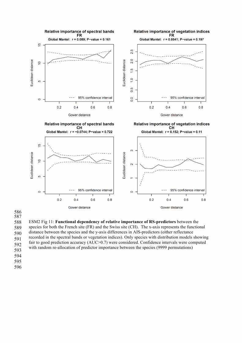
ESM2 Fig 11: Functional dependency of relative importance of RS-predictors between the species for both the French site (FR) and the Swiss site (CH). The x-axis represents the functional distance between the species and the y-axis differences in AIS-predictors (either reflectance recorded in the spectral bands or vegetation indices). Only species with distribution models showing fair to good prediction accuracy (AUC>0.7) were considered. Confidence intervals were computed with random re-allocation of predictor importance between the species (9999 permutations)

597 598 599

ESM2 Fig 12: Phylogenetic dependency of model improvement among species with addition of AIS-predictors for the French site (FR) and the Swiss site (CH). The x-axis represents the phylogenetic distance between the species and the y-axis differences in model improvement when adding AIS-predictors (either reflectance recorded in the spectral bands (BS) or vegetation indices (VI)) to topographic predictors. Confidence intervals were computed with random re-allocation of AUC values between the species (9999 permutations)

600

601

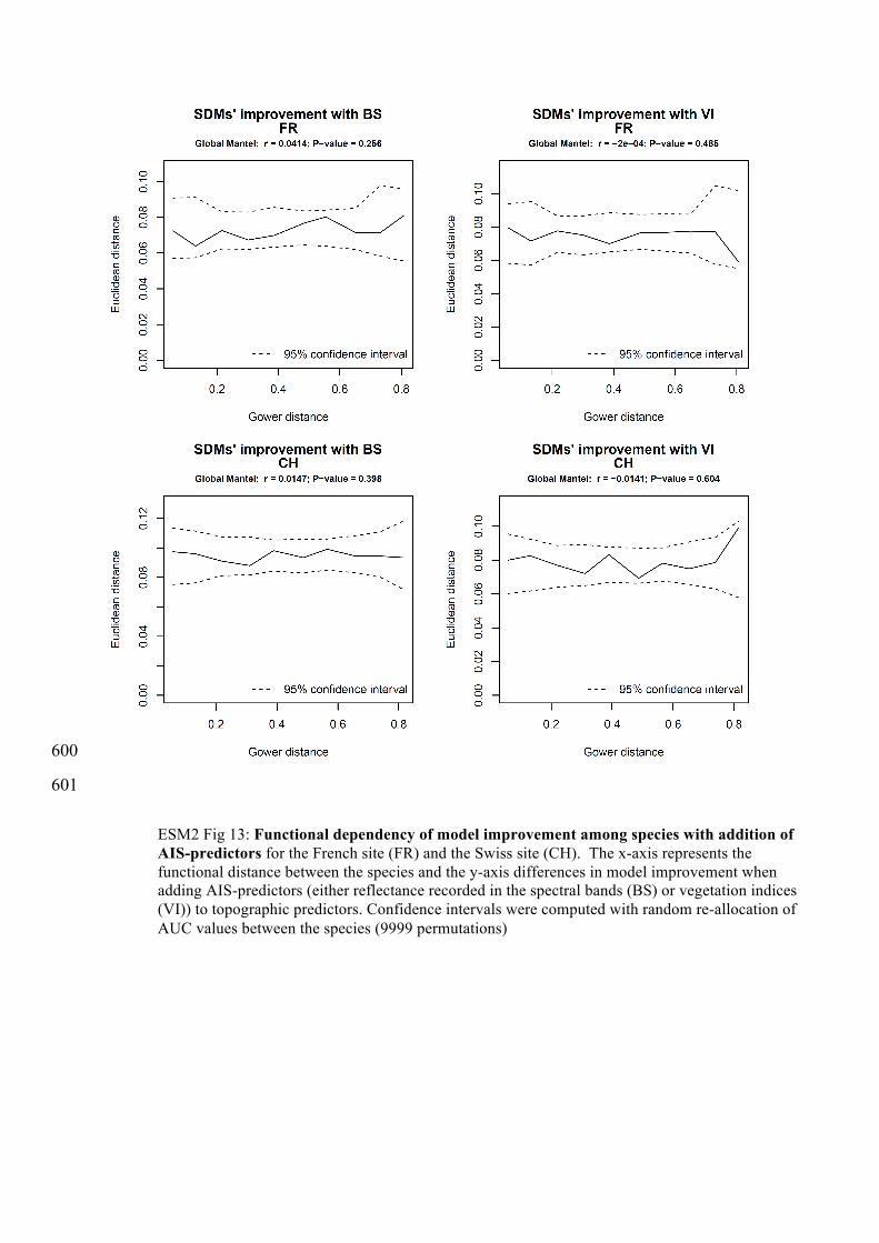
ESM2 Fig 13: Functional dependency of model improvement among species with addition of AIS-predictors for the French site (FR) and the Swiss site (CH). The x-axis represents the functional distance between the species and the y-axis differences in model improvement when adding AIS-predictors (either reflectance recorded in the spectral bands (BS) or vegetation indices (VI)) to topographic predictors. Confidence intervals were computed with random re-allocation of AUC values between the species (9999 permutations)

References 602

1. Hardy, O. J. & Pavoine, S. 2012 Assessing phylogenetic signal with measurement 603 error: a comparison of Mantel tests, Blomberg et al.’s K, and phylogenetic distograms. 604 Evolution 66, 2614–21. (doi:10.1111/j.1558-5646.2012.01623.x) 605

2. Thuiller, W. et al. 2014 Are different facets of plant diversity well protected against 606 climate and land cover changes? A test study in the French Alps. Ecography (Cop.). , 607 Early view. (doi:10.1111/ecog.00670) 608

3. Roquet, C., Thuiller, W. & Lavergne, S. 2013 Building megaphylogenies for 609 macroecology: taking up the challenge. Ecography (Cop.). 36, 13–26. 610 (doi:10.1111/j.1600-0587.2012.07773.x) 611

4. Ndiribe, C., Pellissier, L., Antonelli, S., Dubuis, A., Pottier, J., Vittoz, P., Guisan, A. & 612 Salamin, N. 2013 Phylogenetic plant community structure along elevation is lineage 613 specific. Ecol. Evol. 3, 4925–39. (doi:10.1002/ece3.868) 614

5. Ollinger, S. V 2011 Sources of variability in canopy reflectance and the convergent 615 properties of plants. New Phytol. 189, 375–94. (doi:10.1111/j.1469-616 8137.2010.03536.x) 617

6. Homolová, L., Malenovský, Z., Clevers, J. G. P. W., García-Santos, G. & Schaepman, 618 M. E. 2013 Review of optical-based remote sensing for plant trait mapping. Ecol. 619 Complex. 15, 1–16. (doi:10.1016/j.ecocom.2013.06.003) 620

7. Kleyer, M. et al. 2008 The LEDA Traitbase: a database of life-history traits of the 621 Northwest European flora. J. Ecol. 96, 1266–1274. (doi:10.1111/j.1365-622 2745.2008.01430.x) 623

8. Gower, J. 1971 A general coefficient of similarity and some of its properties. 624 Biometrics 27, 857–871. 625

626

627

Airborne imaging spectroscopy (AIS) can provide remotely sensed estimates of physical and 628 bio-chemical quantitative properties of ecosystems. However, the value of these 629 characteristics for predicting diversity patterns has not been tested yet. We assess the added 630 value of such data for predicting plant distributions in French and Swiss alpine grasslands. We 631 fitted statistical models with high spectral and spatial resolution reflectance data and with four 632 optical indices sensitive to leaf chlorophyll content, leaf water content and leaf area index. We 633 found moderate added value of AIS-data for predicting alpine plant species distribution, 634 revealing issues of scale and AIS-data informational content. 635 636