Modelling of Transport Phenomena in Laser Welding of Steels A. Métais*1,2, S. Matteï1, I. Tomashchuk1 and S. Gaied2 1Laboratoire Interdisciplinaire Carnot de Bourgogne (ICB), UMR 6303 CNRS / Université Bourgogne Franche-Comté, 71200 Le Creusot, FRANCE 2ArcelorMittal, route de Saint Leu 60761 Montataire, FRANCE *alexandre.metais@arcelormittal.com

Abstract: Laser Welded Blank solutions enable to reduce vehicles weight and to optimize their crash performances by means of simultaneous tuning of different grades and thicknesses. The present work aims to characterize numerically and experimentally materials mixing during laser welding. For better understanding of materials mixing based on convection-diffusion process in case of full penetrated laser welding, a 3D simulation of fluid flow, heat transfer and mass transfer has been performed to provide fusion zone shape and elements distribution map. The model has been developed basing on steady keyhole approximation and solved in quasi-stationary form in order to reduce computation time. Turbulent flow model was used to calculate velocity field. Fick law for diluted species was integrated to simulate the transport of alloying elements in the weld pool. In parallel, a number of experiments using pure Ni foils as tracers have been performed to obtain mapping of Ni distribution in the melted zone. SEM-EDX analysis of chemical composition has been made to map elements distribution in the melted zone. The results of simulation have been found in good agreement with experimental data.

Keywords: Laser welding, dissimilar materials, thermo-hydraulic, transport species.

1. Introduction

The role of Laser Welded Blanks (LWB) in vehicles design is significantly increasing. Car manufacturers aim to develop more and more lightweight and strong car architectures that meet latest crash and safety requirements. The main benefits for LWB are mass and cost savings. Mass savings are achieved due to the higher strength level combinations. A good understanding of phenomena occurring during laser welding is essential to obtain a good quality of the weld. Partially penetrated dissimilar laser welding process has already been studied by using heat, fluid flow and transport species inside a 3D model of melt pool [1]. The present study is focusing on a full penetrated laser welding process. The aim of present modelling is to carry out mechanism of formation of eddies in the weld pool by using specific tracers. Then, these

results could be used to improve laser weld mixing between dissimilar steels.

2. Experimental setup

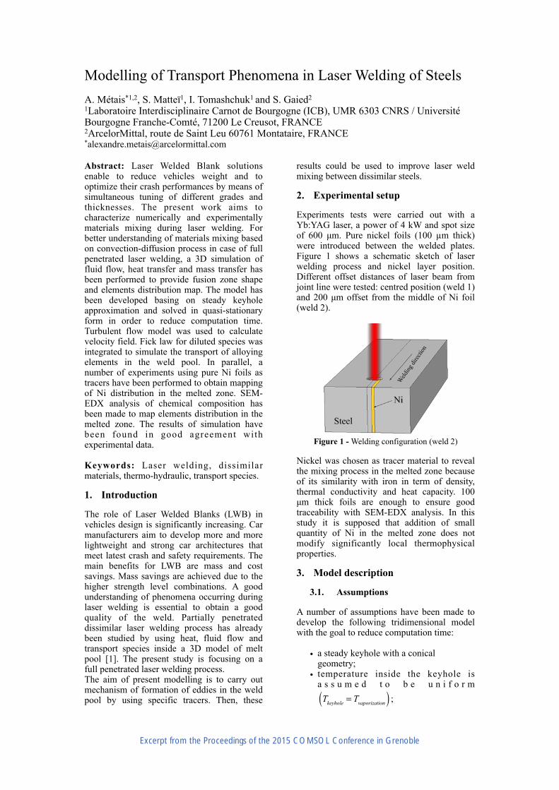
Experiments tests were carried out with a Yb:YAG laser, a power of 4 kW and spot size of 600 µm. Pure nickel foils (100 µm thick) were introduced between the welded plates. Figure 1 shows a schematic sketch of laser welding process and nickel layer position. Different offset distances of laser beam from joint line were tested: centred position (weld 1) and 200 µm offset from the middle of Ni foil (weld 2).

" Figure 1 - Welding configuration (weld 2)

Nickel was chosen as tracer material to reveal the mixing process in the melted zone because of its similarity with iron in term of density, thermal conductivity and heat capacity. 100 µm thick foils are enough to ensure good traceability with SEM-EDX analysis. In this study it is supposed that addition of small quantity of Ni in the melted zone does not modify significantly local thermophysical properties.

3. Model description

3.1. Assumptions

A number of assumptions have been made to develop the following tridimensional model with the goal to reduce computation time:

• a steady keyhole with a conical geometry;

• temperature inside the keyhole is a s s u m e d t o b e u n i f o r m " ; Tkeyhole = Tvaporization( )

Excerpt from the Proceedings of the 2015 COMSOL Conference in Grenoble

• top and bottom surfaces of the weld are assumed to be flat;

• heat transfer and fluid flow equations are strongly coupled;

• liquid metal is assumed to be newtonian and incompressible;

• quasi-steady approach is used.

3.2. Geometry and mesh

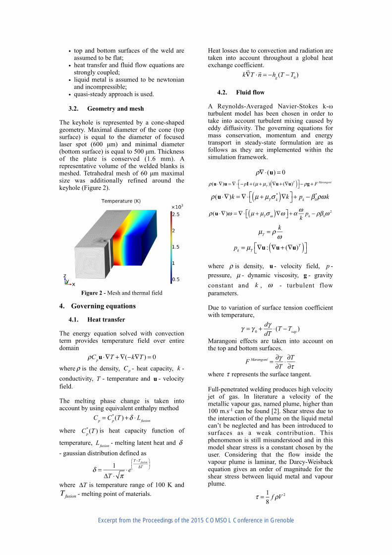
The keyhole is represented by a cone-shaped geometry. Maximal diameter of the cone (top surface) is equal to the diameter of focused laser spot (600 µm) and minimal diameter (bottom surface) is equal to 500 µm. Thickness of the plate is conserved (1.6 mm). A representative volume of the welded blanks is meshed. Tetrahedral mesh of 60 µm maximal size was additionally refined around the keyhole (Figure 2).

" Figure 2 - Mesh and thermal field

4. Governing equations

4.1. Heat transfer

The energy equation solved with convection term provides temperature field over entire domain

"

where" is the density, " - heat capacity, " - conductivity, " - temperature and " - velocity field.

The melting phase change is taken into account by using equivalent enthalpy method

"

where " is heat capacity function of

temperature, " - melting latent heat and "- gaussian distribution defined as

"

where " is temperature range of 100 K and " - melting point of materials.

Heat losses due to convection and radiation are taken into account throughout a global heat exchange coefficient.

"

4.2. Fluid flow

A Reynolds-Averaged Navier-Stokes k-ω turbulent model has been chosen in order to take into account turbulent mixing caused by eddy diffusivity. The governing equations for mass conservation, momentum and energy transport in steady-state formulation are as follows as they are implemented within the simulation framework.

" !

"

"

"

"

where " is density, " - velocity field, " - pressure, " - dynamic viscosity, " - gravity constant and " , " - turbulent flow parameters.

Due to variation of surface tension coefficient with temperature,

"

Marangoni effects are taken into account on the top and bottom surfaces.

"

where " represents the surface tangent.

Full-penetrated welding produces high velocity jet of gas. In literature a velocity of the metallic vapour gas, named plume, higher than 100 m.s-1 can be found [2]. Shear stress due to the interaction of the plume on the liquid metal can’t be neglected and has been introduced to surfaces as a weak contribution. This phenomenon is still misunderstood and in this model shear stress is a constant chosen by the user. Considering that the flow inside the vapour plume is laminar, the Darcy-Weisback equation gives an order of magnitude for the shear stress between liquid metal and vapour plume.

"

ρCpu ⋅∇T +∇(−k∇T ) = 0

ρ Cp kT u

Cp = Cp* (T )+δ ⋅ Lfusion

Cp* (T )

Lfusion δ

δ = 1ΔT ⋅ π

⋅eT−Tfusion

ΔT⎛

⎝⎜

⎞

⎠⎟

ΔTTfusion

k!∇T ⋅ !n = −hg (T −T0 )

ρ∇⋅(u) = 0

ρ(u ⋅∇)u = ∇⋅ − pI + (µ + µT ) ∇u+ (∇u)T( )⎡

⎣⎤⎦ − ρg + F Marangoni

ρ(u ⋅∇)k = ∇⋅ µ + µTσ k*( )∇k⎡

⎣⎤⎦ + pk − β0

*ρωk

ρ(u ⋅∇)ω = ∇⋅ µ + µTσω( )∇ω⎡⎣ ⎤⎦ +αωkpk − ρβ0ω

2

µT = ρ kω

pk = µT ∇u : ∇u+ (∇u)T( )⎡⎣

⎤⎦

ρ u pµ g

k ω

γ = γ 0 +dγdT

⋅(T −Tvap )

F Marangoni = ∂γ∂T

⋅ ∂T∂τ

τ

τ = 18f ρV 2

Excerpt from the Proceedings of the 2015 COMSOL Conference in Grenoble

where " for a laminar flow, " - density

of the plume and " - velocity of the plume. For a velocity of 100 m.s-1 a surface shear stress of 50 N.m2 has been calculated. This value is currently used in our numerical models without experimental validation.

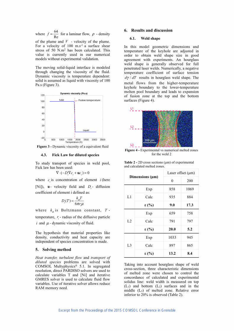
The moving solid-liquid interface is modeled through changing the viscosity of the fluid. Dynamic viscosity is temperature dependent: solid is assumed as liquid with viscosity of 100 Pa.s (Figure 3).

" Figure 3 - Dynamic viscosity of a equivalent fluid

4.3. Fick Law for diluted species

To study transport of species in weld pool, Fick law has been used:

"

where " is concentration of element " (here

[Ni]), " - velocity field and " - diffusion coefficient of element i defined as:

"

where " is Boltzmann constant, " -

temperature, " - radius of the diffusive particle " and " - dynamic viscosity of fluid.

The hypothesis that material properties like density, conductivity and heat capacity are independent of species concentration is made.

5. Solving method

Heat transfer, turbulent flow and transport of diluted species problems are solved with COMSOL Multyphysics® 5.1. In segregated resolution, direct PARDISO solvers are used to calculate variables T and [Ni] and iterative GMRES solver is used to calculate fluid flow variables. Use of iterative solver allows reduce RAM memory need.

6. Results and discussion

6.1. Weld shape

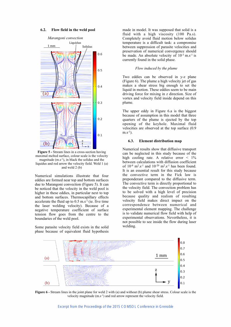
In this model geometric dimensions and temperature of the keyhole are adjusted in order to obtain weld shape size in good agreement with experiments. An hourglass weld shape is generally observed for full penetrated laser welds. Numerically, a negative temperature coefficient of surface tension " results in hourglass weld shape. The metal flows from the higher-temperature keyhole boundary to the lower-temperature molten pool boundary and leads to expansion of fusion zone at the top and the bottom surfaces (Figure 4).

" Figure 4 - Experimental vs numerical melted zones

for the weld 2

Table 2 - 2D cross sections (µm) of experimental and calculated melted zones.

Taking into account hourglass shape of weld cross-section, three characteristic dimensions of melted zone were chosen to control the concordance of calculated and experimental solidus line: weld width is measured on top (L1) and bottom (L2) surfaces and in the middle (L3) of melted zone. Relative error inferior to 20% is observed (Table 2).

f = 64Re

ρ

V

∇⋅(−Di∇ci + uci ) = 0

ci i

u Di

Di(T ) =kBT6πriµ

kB T

rii µ

dγ / dT

Dimensions (µm)Laser offset (µm)

0 200

L1

Exp 858 1069

Calc 935 884

ε (%) 9.0 17.3

L2

Exp 659 758

Calc 791 797

ε (%) 20.0 5.2

L3

Exp 1033 945

Calc 897 865

ε (%) 13.2 8.4

Excerpt from the Proceedings of the 2015 COMSOL Conference in Grenoble

6.2. Flow field in the weld pool

Marangoni convection

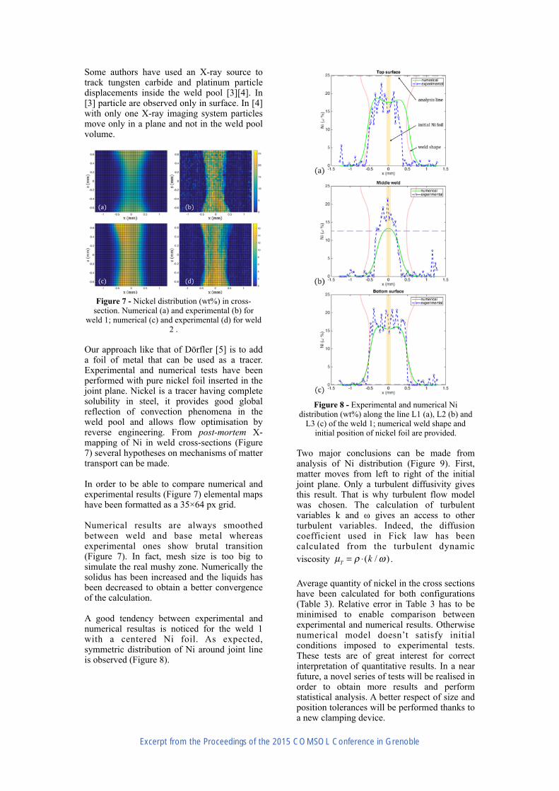
! Figure 5 - Stream lines in a cross-section having

maximal melted surface, colour scale is the velocity magnitude (m.s-1), in black the solidus and the

liquidus and red arrow the velocity field. Weld 1 (a) and weld 2 (b)

Numerical simulations illustrate that four eddies are formed near top and bottom surfaces due to Marangoni convection (Figure 5). It can be noticed that the velocity in the weld pool is higher in these eddies, in particular next to top and bottom surfaces. Thermocapillary effects accelerate the fluid up to 0.5 m.s-1 (ie. five time the laser welding velocity). Because of a negative temperature coefficient of surface tension flow goes from the centre to the boundaries of the weld pool.

Some parasite velocity field exists in the solid phase because of equivalent fluid hypothesis

made in model. It was supposed that solid is a fluid with a high viscosity (100 Pa.s). Completely avoid fluid motion below solidus temperature is a difficult task: a compromise between suppression of parasite velocities and preservation of numerical convergence should be made. An absolute velocity of 10-3 m.s-1 is currently found in the solid phase.

Flow induced by the plume

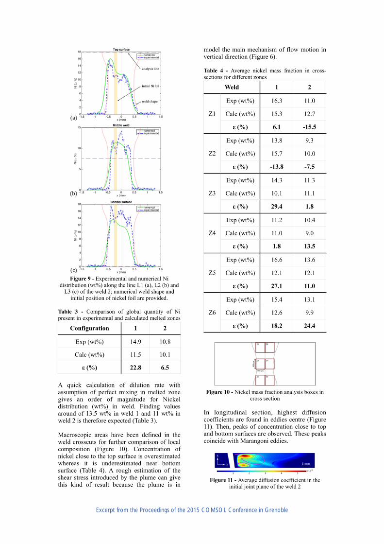
Two eddies can be observed in y-z plane (Figure 6). The plume a high velocity jet of gas makes a shear stress big enough to set the liquid in motion. These eddies seem to be main driving force for mixing in z direction. Size of vortex and velocity field inside depend on this plume.

The upper eddy in Figure 6.a is the biggest because of assumption in this model that three quarters of the plume is ejected by the top opening of the keyhole. Maximal fluid velocities are observed at the top surface (0.9 m.s-1).

6.3. Element distribution map

Numerical results show that diffusive transport can be neglected in this study because of the high cooling rate. A relative error < 1% between calculations with diffusion coefficient of 10-8 m2.s-1 and 10-20 m2.s-1 has been found. It is an essential result for this study because the convective term in the Fick law is preponderant compared to the diffusive term. The convective term is directly proportional to the velocity field. The convection problem has to be solved with a high level of precision because quality and realism of resulting velocity field makes direct impact on the correspondence between numerical and experimental element mapping. The challenge is to validate numerical flow field with help of experimental observations. Nevertheless, it is not possible to see inside the flow during laser welding.

" Figure 6 - Stream lines in the joint plane for weld 2 with (a) and without (b) plume shear stress. Colour scale is the

velocity magnitude (m.s-1) and red arrow represent the velocity field.

Excerpt from the Proceedings of the 2015 COMSOL Conference in Grenoble

Some authors have used an X-ray source to track tungsten carbide and platinum particle displacements inside the weld pool [3][4]. In [3] particle are observed only in surface. In [4] with only one X-ray imaging system particles move only in a plane and not in the weld pool volume.

"

" Figure 7 - Nickel distribution (wt%) in cross-

section. Numerical (a) and experimental (b) for weld 1; numerical (c) and experimental (d) for weld

2 .

Our approach like that of Dörfler [5] is to add a foil of metal that can be used as a tracer. Experimental and numerical tests have been performed with pure nickel foil inserted in the joint plane. Nickel is a tracer having complete solubility in steel, it provides good global reflection of convection phenomena in the weld pool and allows flow optimisation by reverse engineering. From post-mortem X-mapping of Ni in weld cross-sections (Figure 7) several hypotheses on mechanisms of matter transport can be made.

In order to be able to compare numerical and experimental results (Figure 7) elemental maps have been formatted as a 35×64 px grid.

Numerical results are always smoothed between weld and base metal whereas experimental ones show brutal transition (Figure 7). In fact, mesh size is too big to simulate the real mushy zone. Numerically the solidus has been increased and the liquids has been decreased to obtain a better convergence of the calculation.

A good tendency between experimental and numerical resultas is noticed for the weld 1 with a centered Ni foil. As expected, symmetric distribution of Ni around joint line is observed (Figure 8).

" Figure 8 - Experimental and numerical Ni

distribution (wt%) along the line L1 (a), L2 (b) and L3 (c) of the weld 1; numerical weld shape and

initial position of nickel foil are provided.

Two major conclusions can be made from analysis of Ni distribution (Figure 9). First, matter moves from left to right of the initial joint plane. Only a turbulent diffusivity gives this result. That is why turbulent flow model was chosen. The calculation of turbulent variables k and ω gives an access to other turbulent variables. Indeed, the diffusion coefficient used in Fick law has been calculated from the turbulent dynamic viscosity " .

Average quantity of nickel in the cross sections have been calculated for both configurations (Table 3). Relative error in Table 3 has to be minimised to enable comparison between experimental and numerical results. Otherwise numerical model doesn’t satisfy initial conditions imposed to experimental tests. These tests are of great interest for correct interpretation of quantitative results. In a near future, a novel series of tests will be realised in order to obtain more results and perform statistical analysis. A better respect of size and position tolerances will be performed thanks to a new clamping device.

µT = ρ ⋅(k /ω )

Excerpt from the Proceedings of the 2015 COMSOL Conference in Grenoble

" Figure 9 - Experimental and numerical Ni

distribution (wt%) along the line L1 (a), L2 (b) and L3 (c) of the weld 2; numerical weld shape and

initial position of nickel foil are provided.

Table 3 - Comparison of global quantity of Ni present in experimental and calculated melted zones

A quick calculation of dilution rate with assumption of perfect mixing in melted zone gives an order of magnitude for Nickel distribution (wt%) in weld. Finding values around of 13.5 wt% in weld 1 and 11 wt% in weld 2 is therefore expected (Table 3).

Macroscopic areas have been defined in the weld crosscuts for further comparison of local composition (Figure 10). Concentration of nickel close to the top surface is overestimated whereas it is underestimated near bottom surface (Table 4). A rough estimation of the shear stress introduced by the plume can give this kind of result because the plume is in

model the main mechanism of flow motion in vertical direction (Figure 6).

Table 4 - Average nickel mass fraction in cross-sections for different zones

" Figure 10 - Nickel mass fraction analysis boxes in

cross section

In longitudinal section, highest diffusion coefficients are found in eddies centre (Figure 11). Then, peaks of concentration close to top and bottom surfaces are observed. These peaks coincide with Marangoni eddies.

" Figure 11 - Average diffusion coefficient in the

initial joint plane of the weld 2

Configuration 1 2

Exp (wt%) 14.9 10.8

Calc (wt%) 11.5 10.1

ε (%) 22.8 6.5

Weld 1 2

Z1

Exp (wt%) 16.3 11.0

Calc (wt%) 15.3 12.7

ε (%) 6.1 -15.5

Z2

Exp (wt%) 13.8 9.3

Calc (wt%) 15.7 10.0

ε (%) -13.8 -7.5

Z3

Exp (wt%) 14.3 11.3

Calc (wt%) 10.1 11.1

ε (%) 29.4 1.8

Z4

Exp (wt%) 11.2 10.4

Calc (wt%) 11.0 9.0

ε (%) 1.8 13.5

Z5

Exp (wt%) 16.6 13.6

Calc (wt%) 12.1 12.1

ε (%) 27.1 11.0

Z6

Exp (wt%) 15.4 13.1

Calc (wt%) 12.6 9.9

ε (%) 18.2 24.4

Excerpt from the Proceedings of the 2015 COMSOL Conference in Grenoble

Finally, numerical mass conservation was checked. In the transport of diluted species mode, conservative formulation of the Fick law was chosen. Maximum mass loss is of 9.4% (Table 5). It is a satisfying result considering mass conservation equation is roughly calculated in mushy zone and in front of the keyhole.

Table 5 - Nickel mass conservation in Comsol Calculations

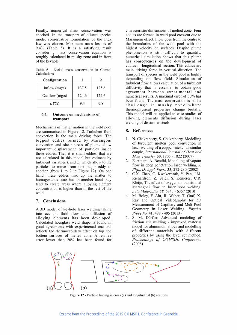
6.4. Outcome on mechanisms of transport

Mechanisms of matter motion in the weld pool are summarised in Figure 12. Turbulent fluid convection is the main driving force. The biggest eddies formed by Marangoni convection and shear stress of plume allow important displacement of particles inside these eddies. Then it is small eddies, that are not calculated in this model but estimate by turbulent variables k and ω, which allow to the particles to move from one major eddy to another (from 1 to 2 in Figure 12). On one hand, these eddies mix up the matter to homogeneous state but on another hand they tend to create areas where alloying element concentration is higher than in the rest of the weld.

7. Conclusions

A 3D model of keyhole laser welding taking into account fluid flow and diffusion of alloying elements has been developed. Calculated hourglass weld shape is found in good agreements with experimental one and reflects the thermocapillary effect on top and bottom surfaces of melted zone. A relative error lower than 20% has been found for

characteristic dimensions of melted zone. Four eddies are formed in weld pool crosscut due to Marangoni effect. Flow goes from the centre to the boundaries of the weld pool with the highest velocity on surfaces. Despite plume phenomenon is still difficult to quantify, numerical simulation shows that this plume has consequences on the development of eddies in longitudinal section. This eddies are main driving force in vertical direction. The transport of species in the weld pool is highly depending on flow field. Simulation of turbulent flow allows calculation of a turbulent diffusivity that is essential to obtain good agreement between experimental and numerical results. A maximal error of 30% has been found. The mass conservation is still a c h a l l e n g e i n m u s h y z o n e w h e r e thermophysical properties change brutally. This model will be applied to case studies of alloying elements diffusion during laser welding of dissimilar steels.

8. References

1. N. Chakraborty, S. Chakraborty, Modelling of turbulent molten pool convection in laser welding of a copper–nickel dissimilar couple, International Journal of Heat and Mass Transfer, 50, 1805 - 1822 (2007)

2. E. Amara, A. Bendid, Modelling of vapour flow in deep penetration laser welding, J. Phys. D: Appl. Phys., 35, 272-280 (2002)

3. C.X. Zhao, C. Kwakernaak, Y. Pan, I.M. Richardson, Z. Saldi, S. Kenjeres, C.R. Kleijn, The effect of oxygen on transitional Marangoni flow in laser spot welding, Acta Materialia, 58, 6345 - 6357 (2010)

4. M. Boley, F. Abt, R. Weber, T. Graf, X-Ray and Optical Videography for 3D Measurement of Capillary and Melt Pool Geometry in Laser Welding, Physics Procedia, 41, 488 - 495 (2013)

5. S. M. Dörfler, Advanced modeling of friction stir welding - improved material model for aluminium alloys and modelling of different materials with different properties by using the level set method, Proceedings of COMSOL Conference (2008)

" Figure 12 - Particle tracing in cross (a) and longitudinal (b) sections

Configuration 1 2

Inflow (mg/s) 137.5 125.6

Outflow (mg/s) 124.6 124.6

ε (%) 9.4 0.8

Excerpt from the Proceedings of the 2015 COMSOL Conference in Grenoble