11th World Congress on Computational Mechanics (WCCM XI)5th European Conference on Computational Mechanics (ECCM V)

6th European Conference on Computational Fluid Dynamics (ECFD VI)E. Onate, J. Oliver and A. Huerta (Eds)

MODELLING OF TIP VORTEX CAVITATION FORENGINEERING APPLICATIONS IN OPENFOAM

Joost J. A. Schot1, Pepijn C. Pennings1, Mathieu J. B. M. Pourquie1, Tom J.C. van Terwisga1

1Technische Universiteit Delft: Fluid Mechanics Section (FM) at the Laboratory for Aero &Hydrodynamics, Mekelweg 2 2628 CD Delft, J.J.A.Schot@student.tudelft.nl,

P.C.Pennings@tudelft.nl, M.J.B.M.Pourquie@tudelft.nl, T.J.C.vanTerwisga@tudelft.nl

Key words: Vortex cavitation, Elliptical planform, OpenFOAM, RANS, Transition,Rotation correction.

Abstract. In this paper modelling assumptions for the prediction of tip vortex flow andvortex cavitation with the RANS equations and homogeneous fluid approach in Open-FOAM are presented. The effects of the changes in the turbulence model are investigatedand the results are compared with PIV measurements.

1 INTRODUCTION

Tip vortex cavitation has been studied extensively for a wing with an elliptical planformwith an aspect ratio of 3 and a NACA 662 − 415 cross-sectional shape using an a = 0.8mean line [1]. It was found that at certain cavitation numbers the tip vortex cavitytrailing from this wing emits a strong tonal noise, called vortex singing [2]. The cause ofthe singing behaviour of the vortex cavity is not yet known, but most likely related toexcitement of one of its natural vibration modes, described by [3], due to flow instabilitiesin the tip region. This singing behaviour is of particular interest as it is one of the possibleexplanations of the high frequency broadband noise generated by skewed ship propellers,designed to avoid sheet cavitation [4].

The conventional modelling approach for cavitation problems in engineering applica-tions is with a first order closure Reynolds averaged Navier-Stokes (RANS) model. Themulti-phase aspects are included with the homogeneous fluid approach, the volume offluid (VOF) method and a mass transfer model. It is known that most of these turbu-lence models need corrections in rotational flows. Other methods, such as a ReynoldsStress Transport Model (RSTM) or Large Eddy Simulations (LES) increase the computa-tional time enormously, especially when the boundary layer needs to be resolved. Furthercomplications arise when transition of the boundary layer is important, which is the casefor the wing in the present study. Therefore, vortex cavitation is approximated with a

1

Joost J. A. Schot, Pepijn C. Pennings, Mathieu J. B. M. Pourquie, Tom J. C. van Terwisga

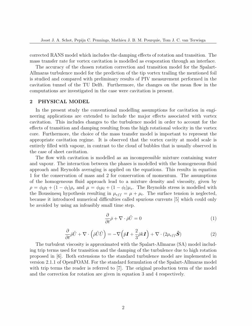
corrected RANS model which includes the damping effects of rotation and transition. Themass transfer rate for vortex cavitation is modelled as evaporation through an interface.

The accuracy of the chosen rotation correction and transition model for the Spalart-Allmaras turbulence model for the prediction of the tip vortex trailing the mentioned foilis studied and compared with preliminary results of PIV measurement performed in thecavitation tunnel of the TU Delft. Furthermore, the changes on the mean flow in thecomputations are investigated in the case were cavitation is present.

2 PHYSICAL MODEL

In the present study the conventional modelling assumptions for cavitation in engi-neering applications are extended to include the major effects associated with vortexcavitation. This includes changes to the turbulence model in order to account for theeffects of transition and damping resulting from the high rotational velocity in the vortexcore. Furthermore, the choice of the mass transfer model is important to represent theappropriate cavitation regime. It is observed that the vortex cavity at model scale isentirely filled with vapour, in contrast to the cloud of bubbles that is usually observed inthe case of sheet cavitation.

The flow with cavitation is modelled as an incompressible mixture containing waterand vapour. The interaction between the phases is modelled with the homogeneous fluidapproach and Reynolds averaging is applied on the equations. This results in equation1 for the conservation of mass and 2 for conservation of momentum. The assumptionsof the homogeneous fluid approach lead to a mixture density and viscosity, given byρ = φlρl + (1 − φl)ρv and µ = φlµl + (1 − φl)µv. The Reynolds stress is modelled withthe Boussinesq hypothesis resulting in µeff = µ + µt. The surface tension is neglected,because it introduced numerical difficulties called spurious currents [5] which could onlybe avoided by using an infeasibly small time step.

∂

∂tρ+∇ · ρU = 0 (1)

∂

∂tρU +∇ ·

(ρU U

)= −∇

(pI +

2

3ρkI

)+∇ · (2µeff S) (2)

The turbulent viscosity is approximated with the Spalart-Allmaras (SA) model includ-ing trip terms used for transition and the damping of the turbulence due to high rotationproposed in [6]. Both extensions to the standard turbulence model are implemented inversion 2.1.1 of OpenFOAM. For the standard formulation of the Spalart-Allmaras modelwith trip terms the reader is referred to [7]. The original production term of the modeland the correction for rotation are given in equation 3 and 4 respectively.

2

Joost J. A. Schot, Pepijn C. Pennings, Mathieu J. B. M. Pourquie, Tom J. C. van Terwisga

The correction for the damping effects of rotation changes the component Ω of S shownin equation 3 of the production term Cb1(1 − ft2)Sν in Ω∗. This introduces a dampingrate depending on the empirical constant Crot when the magnitude of the rate-of-rotationtensor exceeds the magnitude of the rate-of-strain tensor.

S =Ω +ν

κ2d2fv2

Ω = |2Ω|(3)

Ω∗ = Ω + Crotmin(0, |2S| − Ω) (4)

The Volume Of Fluid (VOF) method is used to track the interface (eqn. 5). Themass transfer rate is based on the Langmuir mass transfer rate through an interface andthe area density of the interface is approximated with a global estimate of the local gridspacing (eqn. 6).

∂φl∂t

+∇ · (φlU) =1

ρlΓl (5)

Γl = Ad CLangmuir (p− pv) ∼10−3

∆x(p− pv)

kg

m3s(6)

3 NUMERICAL MODEL

The numerical methods of OpenFOAM are used in this study, which applies the finitevolume method to discretize the equations. The spatial accuracy is limited to second order,as a result of the approximation of the divergence term after applying Gauss’ theoremwhich is of this order. Furthermore, no stable higher order schemes are included for theinterpolation of the face values. This leads to a numerical viscosity of the order of thefluid viscosity for a study on the analytical Taylor-Green vortex with similar propertiesas the vortex trailing the wing in the present study [8].

The solver simpleFoam is used for the steady-state fully wetted computations. Forthe interpolation of the face values for the convective term of the momentum equationthe ’linearUpwindV’ scheme is used. For the face values for the convective term of theturbulence model the ’limitedLinear’ scheme is used. Other face values are interpolatedwith the ’linear’ scheme.

For the steady-state cavitating computations the interPhaseChangeFoam solver is ap-plied with the same interpolation schemes. The temporal discretisation is performed withthe local time stepping scheme of OpenFoam ’localEuler’. For the interpolation of theliquid fraction near the interface the ’SuperBee’ scheme is used and the interface compres-sion coefficient (Cλ) of OpenFOAM is set to 1. For the time step the advised maximumCourant number of 0.2 is used.

3

Joost J. A. Schot, Pepijn C. Pennings, Mathieu J. B. M. Pourquie, Tom J. C. van Terwisga

4 RESULTS

First the computational domain and grid are described. The transition is applied ona specified line approximated by transition locations predicted by xFoil at two locationsalong the span of the wing and the mid chord position at the tip. First fully wettedsteady state computations are discussed with the Spalart-Allmaras model with rotationcorrection (SA-R) and the model with transition terms (SA-R-trip). Then the effects ofcavitation are discussed, at a cavitation number of 1.7 which was chosen to avoid thepresence of sheet cavitation.

4.1 Computational domain

The computational domain has the same dimensions as the test section of the cavitationtunnel at the TU Delft and is shown in figure 1. The wing has been set at a geometricalangle of attack (αg) of 9 degrees, in order to avoid the difficulty of resolving the laminarseparation bubble which forms at lower angles of attack. The chord length of the wing(c) is 125.6 mm. The half span (1

2b) is equal to 150 mm. The trailing edge has been cut

off with a thickness of 0.3 mm. It should be noted that for the line plots shown later ona local coordinate system has been used.

Figure 1: Computational domain, similar to the test section of the cavitation tunnel at the TU Delft.The flow is from left to right.

The test case was conducted at a Reynolds number of 6.8 105, which corresponds toan inlet velocity of 5.43 m

s. The kinematic viscosity is set to be 1.0034 · 10−6m

2

s, which

corresponds to fresh water at a temperature of 20 Celsius. The density of the liquid is998.2 kg

m3 and the vapour pressure 2339.3Pa [9]. For the cavitating case the vapour density

of 0.01731 kgm3 and kinematic viscosity of 561.84 · 10−6m

2

sare used for water vapour at the

same temperature at vapour pressure based on the IAPWS-IF97 table [10].

4.2 Computational grid

For the computations an unstructured grid has been generated with approximately 25million cells with around 15 cells over the viscous core of the vortex for the fully turbulent

4

Joost J. A. Schot, Pepijn C. Pennings, Mathieu J. B. M. Pourquie, Tom J. C. van Terwisga

case. The case with a laminar boundary layer section has approximately 10 cells over thecore. The grid near the root at the trailing edge and leading edge is shown in figure 2and 3. The refinement near the vortex core at the tip is shown in figure 4. The boundarylayer on the wing is fully resolved with a maximum y+ value of around 2.

Figure 2: Grid refinementnear the trailing edge at theroot of the wing.

Figure 3: Grid refinementnear the leading edge at theroot of the wing.

Figure 4: Grid refinement inthe tip vortex region near thetip of the wing.

4.3 Surface flow pattern and integral quantities

First the flow over the wing is compared with experiments in figure 5 and 6. It is ob-served that for the case with early transition the general flow pattern agrees qualitativelywith oil visualisation experiments [11], but a laminar separation bubble at lower anglesof attack can not be reproduced.

Figure 5: Pressure coefficient and surface stream-lines based on the wall friction on the suction sidecomputed with the SA-R model.

Figure 6: Oil visualization of surface streamlineswith early transition at αg = 10 and Re = 5.3 105

[11].

The result of the laminar separation bubble, which can still be present at αg = 9 inexperiments, is a decrease in the lift coefficient. This is visible in the experimental valuesin table 1. When the results are compared with thin airfoil theory based on the experi-mentally observed range of zero lift angles it shows agreement with the computations.

5

Joost J. A. Schot, Pepijn C. Pennings, Mathieu J. B. M. Pourquie, Tom J. C. van Terwisga

Table 1: Comparison of the predicted lift and drag coefficient with experiments.

Cl Cdi Cd − CdiSA-R 0.72 0.055 0.010

SA-R-trip 0.74 0.058 0.007Exp. [1] 0.64 0.043 0.033

Exp. TU Delft 0.56 - -Thin airfoil theory 0.71± 0.04 - -

4.4 Effects of the rotation corrections

The turbulence production in the core of the vortex is damped by the correction to theSA model given in equation 4, referred to as the SA-R model. In figure 7 the effect on theproduction term in a cross section of the vortex is shown at one chord length downstreamof the tip. It is observed that damping is present in the vortex core and the shear layerrolling up into it. The damping of the production is at a rate proportional to the empiricalconstant Crot and isotropic. However, in turbulent vortices it is observed that mainly theradial turbulent fluctuations are damped [12] and not the other components.

The production of turbulence resulting from the gradient of the axial velocity is notpresent with this correction. This effect is shown in figure 8 where it can be seen thatthe production term is highly damped in the region where the gradient in axial velocity(Ωxy) is large. The contributions to the magnitude of the mean rate-of-rotation tensor isgiven in equation 7.

|2Ω|2 = 2Ω2xy + 2Ω2

xz + 2Ω2yz (7)

Figure 7: The corrected production term asa percentage of the original production term,shown at one chord length downstream of thetip of the wing in the traverse direction look-ing upstream.

−5 −4 −3 −2 −1 0 1 2 3 4 50

25

50

75

100

y[mm]

[%]

Ω2xy|Ω|

−2max

Ω2xz|Ω|

−2max

Ω2yz |Ω|

−2max

|Ω|2|Ω|−2max

Ω−2.0min(0,|2S|−Ω)Ω

Figure 8: Contribution of the distinct term of the meanrate-of-rotation tensor to its magnitude and the dampedproduction term of the SA-R model. The results areshown one chord length downstream of the wing tip look-ing downstream in the traverse direction over the horizon-tal axis.

6

Joost J. A. Schot, Pepijn C. Pennings, Mathieu J. B. M. Pourquie, Tom J. C. van Terwisga

4.5 Effects of the inclusion of transition

Experiments suggest [13] that the core radius is a function of the boundary layerthickness, as in equation 8. For a fully turbulent boundary layer the value n = 0.2, basedon the turbulent boundary layer thickness formulation. In experiments a value of n = 0.4has been found by McCormick, which is explained by the transitional boundary layeron the wing [14]. It is therefore expected that the viscous core radius is affected by theinclusion of transition in the turbulence model.

rc ∼ δb ∼ cRe−n (8)

The effect of transition on the growth of the viscous core and magnitude of the cir-culation within five viscous core radii at different locations downstream of the tip of thewing is shown in figure 9 and 10 respectively. It is observed that the circulation, nor-malized with the estimated circulation at the root (based on a lift coefficient of 0.71) ofΓ0 = 0.24m

2

s, is very similar to what is found in experiments on other section shapes with

an elliptical planform [13]. The growth of the viscous core radius scales with√νappt,

where t = xU∞

, which is also shown with the estimated apparent viscosity of both casesin figure 9. The computation which includes transition produces better agreement withmeasurements.

Figure 9: Growth of the radius of the viscous coresize at different locations downstream of the tip ofthe wing. The lines give the approximated growthbased on

√νappt from x

c = 0.2.

Figure 10: The circulation at different locationsdownstream of the tip of the wing, within five vis-cous core radii from the center of the vortex.

Further investigation of the turbulent viscosity in the roll-up region suggests a complexscaling of the viscous core radius. The boundary layer thickness and turbulent viscosityconvecting from the wing are first affected by the shear layer forming in the wake ofthe wing. Then this shear layer enters the vortex in the roll-up process, where the highrotation begins to dampen the turbulent viscosity. This process is shown in figure 11 forboth cases.

7

Joost J. A. Schot, Pepijn C. Pennings, Mathieu J. B. M. Pourquie, Tom J. C. van Terwisga

Figure 11: Turbulent viscosity in the roll-up region comparing the SA-R model on the left and theSA-R-trip model on the right. It is observed that the delayed transition decreases the turbulent viscositysignificantly.

4.6 Effects of cavitation

When cavitation is introduced it is observed that the flow pattern in the vortex changessignificantly. The circumferential velocity no longer follows the solid-body rotation profileas in the fully wetted flow. This is shown in figure 12, where also the PIV measurementsfor fully wetted flow are shown. There is a change in the velocity gradient close to theedge of the cavity, which might be related to the non-zero mass transfer in this region.

−15.0 −12.5 −10.0 −7.5 −5.0 −2.5 0.0 2.5 5.0 7.5 10.0 12.5 15.0−5.00

−4.00

−3.00

−2.00

−1.00

0.00

1.00

2.00

3.00

4.00

5.00

y[mm]

w[ms]

Cavitating σ = 1.7Fully wettedPIV results

Figure 12: Circumferential velocity at one chord length behind the tip looking downstream in traversedirection over the horizontal axis. A schematic representation of the effect of cavitation is presented onthe right, where a radial velocity resulting from local mass transfer is visible and a change in velocitygradient at the interface between the vapour and liquid.

Mass transfer leads to divergence of the velocity field as given in equation 9. The masstransfer is indicated with figure 14 where the red line gives the divergence of the velocity,which is non-zero near the edge of the cavity. The main contribution is found to be Syy,which is the radial gradient of the radial velocity component. The largest components ofthe mean rate-of-strain tensor are shown in figure 13.

∇ · U =( 1

ρl− 1

ρv

)Γl (9)

S =1

2

Sxx Sxy SxzSyx Syy SyzSzx Szy Szz

=1

2

2∂u∂x

∂u∂y

+ ∂v∂x

∂u∂z

+ ∂w∂x

∂v∂x

+ ∂u∂y

2∂v∂y

∂v∂z

+ ∂w∂y

∂w∂x

+ ∂u∂z

∂w∂y

+ ∂v∂z

2∂w∂z

(10)

8

Joost J. A. Schot, Pepijn C. Pennings, Mathieu J. B. M. Pourquie, Tom J. C. van Terwisga

−2.5 −2.0 −1.5 −1.0 −0.5 0.0 0.5 1.0 1.5 2.0 2.50

10

20

30

40

50

60

70

80

90

100

y[mm]

[%]

2|Sxy|2|S|−2

max

2|Syz|2|S|−2

max

|Syy|2|S|−2

max

|S|2|S|−2max

φl

Figure 13: Magnitude of the rate-of-strain tensor,its largest components and the liquid fraction atone chord length downstream of the tip along thetransverse horizontal line looking downstream.

−2.5 −2.0 −1.5 −1.0 −0.5 0.0 0.5 1.0 1.5 2.0 2.50

10

20

30

40

50

60

70

80

90

100

y[mm]

[%]

|Sxx + Syy + Szz|2|S|−2

max

|Syy|2|S|−2

max

|Szz|2|S|−2

max

|S|2|S|−2max

φl

Figure 14: Magnitude of the rate-of-strain tensor,the components resulting from divergence of the ve-locity vector and the liquid fraction at one chordlength downstream of the tip along the transversehorizontal line looking downstream.

In the viscous core the pressure reduction vanishes inside the cavity if present, whichcan be seen in figure 15. This is due to the low density of vapour compared to that of

the liquid, as it decreases with a factor 6 · 104. The centrifugal component −ρu2θ

rin the

conservation of radial momentum (eqn. 11) is approximately balanced by the pressuregradient as shear and radial velocity are small in a solid-body rotation region. Thecentrifugal component is reduced due to the density difference.

ρ(ur∂ur∂r− u2θ

r

)= −∂p

∂r+ µ(∇2ur −

urr2)

(11)

−10 −9 −8 −7 −6 −5 −4 −3 −2 −1 0 1 2 3 4 5 6 7 8 9 10−2.50

−2.00

−1.50

−1.00

−0.50

0.00

y[mm]

Cp

Cavitating σ = 1.7Fully wetted

Figure 15: Pressure coefficient at one chord lengthbehind the tip looking downstream along the hori-zontal axis.

The axial velocity in the core of a vortex is a result of the axial pressure gradient, whichdepends for a non-cavitating vortex on the growth of the core, gain in circulation in theroll-up process and effects of the boundary layer [15]. When cavitation is present thecore pressure is very close to vapour pressure and the axial pressure gradient is thereforelikely to be reduced in this region. This leads to the difference in the axial velocity

9

Joost J. A. Schot, Pepijn C. Pennings, Mathieu J. B. M. Pourquie, Tom J. C. van Terwisga

pattern shown in figure 16. It is however observed in both the PIV measurements and inexperiments by [1] that the axial velocity is increased instead of decreased at this location.The difference is likely caused by numerical diffusion and the approximation within therotations correction.

−10 −9 −8 −7 −6 −5 −4 −3 −2 −1 0 1 2 3 4 5 6 7 8 9 100.60

0.70

0.80

0.90

1.00

1.10

1.20

1.30

y[mm]

u

u∞

Cavitating σ = 1.7Fully wetted

Figure 16: Axial velocity normalized by the free stream velocity at one chord length behind the tiplooking downstream along the traverse horizontal line. A schematic representation of the effect of cavi-tation is presented on the right, where the reduction of the pressure gradient in the vapour core reducesthe driving mechanism for the axial flow in that region.

5 CONCLUSIONS

The present study investigates the capabilities of OpenFOAM to predict steady tipvortex cavitation. It was found in a previous study that the simulation of a tip vortexflow with OpenFOAM is hampered by the numerical diffusion as a result of the secondorder accurate spatial discretisation [8]. This leads to an estimated numerical viscosity ofthe order of the fluid viscosity in the vortex.

The inclusion of the damping on the turbulence resulting from the high rotation in thevortex was necessary to avoid an excessive spreading of the vortex core. This correctionreduces the turbulent viscosity to the same order as the fluid viscosity, making the nu-merical error and the amount of turbulence damping important for the prediction of thegrowth of the core.

Also the modelling of transition of the boundary layer affects the viscous core size ofthe vortex as a result of its turbulent viscosity rolling up in the vortex core. This is alteredin the shear layer trailing the wing and damped when it rolls up in the vortex core.

It is concluded that for lower angles of attack laminar separation should be taken intoaccount on this wing and that the empirical damping constant Crot is not expected tomimic a physical damping rate. It is observed that the circumferential velocity profile,the core radius and circulation agree with the PIV measurements. However, the measuredlift coefficient at the same conditions was significantly lower at about 0.56 affecting thestrength of the vortex.

When cavitation is included in the simulation it is observed that the velocity profileof the vortex changes significantly. At the interface of the cavity there is mass transfer

10

Joost J. A. Schot, Pepijn C. Pennings, Mathieu J. B. M. Pourquie, Tom J. C. van Terwisga

and there is a change in circumferential velocity gradient present at this location in thesolid-body rotation region. As a result of the large density difference of the water andvapour, the decrease in pressure is very small inside the vapour cavity. This likely leadsto a reduction of the axial velocity in the vapour core of the vortex.

6 ACKNOWLEDGEMENTS

The developers of OpenFoam are gratefully acknowledged for making the CFD toolavailable. Furthermore, the Fluid Mechanics Section (FM) at the Laboratory for Aero &Hydrodynamics of the TU Delft is thanked for providing the resources for the computa-tions.

LIST OF SYMBOLS

Ω Mean rate-of-rotation tensor(12

(∇U −∇UT

))S Mean rate-of-strain tensor

(12

(∇U +∇UT

))∆x Local grid spacing

δb Boundary layer thickness

Γl Mass transfer rate of the liquid phase

φl Liquid fraction

Ad Area density( ∫∞−∞Addn = 1

)b Wingspan from tip to tip

c Cord length

Cλ Interface compression coefficient

Cdi Induced drag estimated with Cdi =C2L

πAR

CLangmuir Mass transfer constant in the Langmuir evaporation equation

Crot Rotation constant of the SA-R model

Re Reynolds number(uLν

)y+ Distance form the wall normalized by the viscous length scale

REFERENCES

[1] R. E. A. Arndt and A. P. Keller. Water Quality Effects on Cavitation Inception in aTrailing Vortex. ASME, Vol. 114, 430–438, 1992.

[2] B. Maines and R. E. A. Arndt. The Case of the Singing Vortex. J. Fluids Eng., Vol.119, 271–276, 1997.

11

Joost J. A. Schot, Pepijn C. Pennings, Mathieu J. B. M. Pourquie, Tom J. C. van Terwisga

[3] J. Bosschers. Investigation of the resonance frequency of a cavitating vortex.NAG/DAGA, The Netherlands, Rotterdam, 289–291, 2009.

[4] E. van Wijngaarden, J. Bosschers and G. Kuiper. Aspects of the cavitating propellertip vortex as a source of inboard noise and vibration. Proceedings of FEDSM2005,Houston, TX, USA, 2005.

[5] S. S. Deshpande, L. Anumolu and M. Trujillo. Evaluation the performance of thetwo-phase flow solver inter-Foam. Computational science & discovery, Vol. 5, 1–36,2012.

[6] J. Dacles-Mariani, D. Kwak and G. Zilliac. On Numerical Errors and TurbulenceModeling in Tip Vortex Flow Prediction. Int. J. Numer. Meth. Fluids, Vol. 30, 65-82, 1999.

[7] P. R. Spalart, S. R. Allmaras. A one-equation turbulence model for aerodynamicflows. 30th Aerospace sciences meeting & exhibit, 1–22, 1992.

[8] J. J. A. Schot. Numerical study of vortex cavitation on the elliptical Arndt foil. M.Sc.Thesis. Technische Universiteit Delft: The Netherlands, 2014.

[9] ITTC. ITTC Recommended Procedures, Fresh Water and Seawater Properties. 2011.

[10] J. R. Cooper, R. B. Dooley. Revised Release on the IAPWS Industrial Formulation1997 for the Thermodynamic Properties of Water and Steam. The InternationalAssociation for the Properties of Water and Steam, 1997.

[11] R. E. A. Arndt, V. H. Arakeri and H. Higuchi. Some observations of tip-vortexcavitation. Journal of fluid mechanics, Vol. 229, 269–289, 1991.

[12] J. S. Chow, G. G. Zilliac and P. Bradshaw. Turbulence measurements in the near-fieldof a wingtip vortex. NASA TM, 1997.

[13] J. A. Astolfi, D. H. Fruman and J. Y. Billard. A model for tip vortex roll-up in thenear field region of three-dimensional foils and the prediction of cavitation onset.European Journal of Mechanics - B/Fluids, Vol. 18, 757-775, 1999.

[14] B. H. Maines and R. E. A. Arndt. Tip vortex formation and cavitation. Journal offluid mechanics, Vol. 119, 413-419, 1997.

[15] G. K. Batchelor. Axial flow in trailing line vortices. Journal of Fluid Mechanics, Vol.20, 645–658, 1964.

12