CHEMICAL REACTION ENGINEERING LABORATORY Bubble and Slurry columns.

HAL Id: tel-02006754https://tel.archives-ouvertes.fr/tel-02006754
Submitted on 4 Feb 2019
HAL is a multi-disciplinary open accessarchive for the deposit and dissemination of sci-entific research documents, whether they are pub-lished or not. The documents may come fromteaching and research institutions in France orabroad, or from public or private research centers.
L’archive ouverte pluridisciplinaire HAL, estdestinée au dépôt et à la diffusion de documentsscientifiques de niveau recherche, publiés ou non,émanant des établissements d’enseignement et derecherche français ou étrangers, des laboratoirespublics ou privés.
Modelling of the hydrodynamics of bubble columnsusing a two-fluid model coupled with a population
balance approachLuca Gemello
To cite this version:Luca Gemello. Modelling of the hydrodynamics of bubble columns using a two-fluid model coupledwith a population balance approach. Fluid mechanics [physics.class-ph]. Université de Lyon; Politec-nico di Torino, 2018. English. �NNT : 2018LYSE1245�. �tel-02006754�

5

Doctoral Dissertation
Université Claude Bernard Lyon 1 - ED 162 MEGAPolitecnico di Torino - Chemical Engineering
Prepared in the laboratory of IFP Energies nouvelles
Speciality: Chemical Engineering and Fluid Mechanics
Modelling of the hydrodynamics of bubblecolumns using a two-fluid model coupled
with a population balance approach
Luca Gemello
SupervisorsFrédéric Augier, Supervisor UCB Lyon 1 - IFP Energies nouvelles
Daniele Marchisio, Supervisor Politecnico di TorinoCécile Plais, Co-supervisor IFP Energies nouvelles
Doctoral Examination CommitteeDavid FLETCHER, The University of Sidney, ReviewerVeronique ROIG, INP Toulouse, ReviewerFrédéric AUGIER, UCB Lyon 1 - IFP Energies nouvelles, SupervisorDaniele MARCHISIO, Supervisor Politecnico di Torino, SupervisorCécile PLAIS, IFP Energies nouvelles, Co-supervisorPascal FONGARLAND, UCB Lyon 1Micheline ABBAS, Université Toulouse IIIGiuseppina MONTANTE, Università di Bologna
1

2

Abstract
Modelling of the hydrodynamics of bubble columns using atwo-fluid model coupled with a population balance approach
The simulation of bubble column reactors under industrial operating conditions isan exciting challenge. The main objective of this work is to predict the bubble size,in turn interconnected with the reactor hydrodynamic conditions, with computa-tional models, by modelling bubble breakage and coalescence. Experimental dataare collected for model validation, including bubble size measurements with an in-novative cross-correlation technique. Experiments are carried out with tap waterand demineralised water, with or without the addition of ethanol, and gatheredresults show that additives reduce coalescence and lower the mean bubble size.Two different spargers are used, in order to decouple the investigation of breakageand coalescence. The experimental data set is used to validate our unsteady three-dimensional Eulerian-Eulerian CFD simulations. A drag law for oblate bubblesis considered, together with a factor that accounts for the swarm effect. Severalturbulence models are tested. The contribution of the bubbles to scalar mixingis assessed. To predict bubble size, a population balance model is coupled to thehydrodynamic model and is solved with the quadrature method of moments. A setof breakage and coalescence kernels is proposed, capable of predicting the bubblesize for different operating conditions. Scale-up effects are also investigated.
Keywords Bubble columns, Bubble size, Computational fluid dynamics, Popu-lation balance modelling, QMOM.
3

4

Résumé
Modélisation de l’hydrodynamique des colonnes à bulles selonune approche couplant modèle à deux fluides et bilan depopulation
La simulation de réacteurs à bulles en régime industriel est un grand défi. L’objectifprincipal de ce travail est la prédiction de la taille des bulles à l’aide d’un modèlenumérique de bilan de population, basé sur la modélisation des phénomènes debrisure et de coalescence, et pouvant être couplé aux conditions hydrodynamiquesprésentes dans les réacteurs. Différentes données expérimentales sont obtenuespour valider le modèle. La taille des bulles est mesurée à l’aide d’une techniqueinnovante de corrélation croisée. Les essais, réalisés en eau du réseau (partiellementcontaminée) et en eau déminéralisée avec ajout éventuel d’éthanol, montrent que lesadditifs réduisent la coalescence et diminuent la taille moyenne des bulles. Deuxdistributeurs du gaz différents sont utilisés pour découpler l’étude de la bri-sureet de la coalescence. Les données expérimentales sont utilisées initialement pourvalider des simulations CFD 3D transitoires Eulériennes-Eulériennes. La loi detraînée est corrigée par un facteur de swarm pour intégrer l’effet d’une fractionde gaz élevée. Différents modèles de turbulence sont testés. La contribution desbulles au mélange de scalaires est évaluée. Enfin, pour prédire la taille des bulles,un bilan de population est couplé au modèle hydrodynamique préalablement validéet est résolu par la méthode de quadrature des moments (QMOM). Un set originalde kernels de brisure et coalescence est proposé, capable de prédire la taille desbulles pour différentes conditions opératoires. Le comportement du modèle lors del’extrapolation des réacteurs est également examiné.
Mots clés Colonnes à bulles, Taille des bulles, CFD, Bilan de population, QMOM.
5

6

Riassunto
Modellazione dell’idrodinamica delle colonne a bolle con unapproccio che combina modello a due fluidi e bilancio dipopolazione
La simulazione di colonne a bolle in condizioni industriali è un problema di granderilevanza. L’obiettivo principale di questo lavoro è prevedere con modelli com-putazionali la dimensione delle bolle, legata alla fluidodinamica dei reattori, con-siderando i fenomeni di rottura e di coalescenza. La validazione del modello èeffettuata tramite il confronto con dati sperimentali appositamente raccolti, tra cuila dimensione delle bolle, ottenuta con un’innovativa tecnica di cross-correlazione.Gli esperimenti effettuati con acqua parzialmente contaminata e con acqua demi-neralizzata con l’eventuale aggiunta di etanolo, mostrano che gli additivi riduconola coalescenza e diminuiscono la dimensione media delle bolle. Sono stati inoltreutilizzati negli esperimenti con due sparger diversi, per disaccoppiare lo studiodi rottura e coalescenza. I dati sperimentali sono stati utilizzati per convalidaresimulazioni CFD 3D transitorie Euleriane-Euleriane. Il modello per la forza ditrascinamento è corretto da un fattore di swarm per considerare l’effetto delle in-terazioni tra le bolle. Sono stati testati diversi modelli di turbolenza, nonché ilcontributo delle bolle sulla miscelazione degli scalari. Per prevedere la dimensionedelle bolle, è stato utilizzato un bilancio di popolazione risolto con il metodo diquadratura dei momenti. Nella presente tesi viene proposto un set di kernel dirottura e coalescenza per prevedere le dimensioni delle bolle in diverse condizionioperative, considerando anche gli effetti dello scale-up.
Parole chiave Colonne a bolle, Dimensione delle bolle, CFD, Bilancio di popolazione,QMOM.
7

8

Résumé substantiel
Cette thèse de doctorat porte sur la modélisation des réacteurs à bulles en ré-gime industriel. L’objectif principal est la prédiction et la modélisation de la tailledes bulles dans ces systèmes. Parmi les différents types de réacteurs gaz-liquide,les colonnes à bulles sont largement utilisées dans différents domaines du géniechimique. La géométrie de ces réacteurs est simple, sans parties mobiles. Lescolonnes à bulles ont de faibles coûts d’exploitation et d’entretien et de bons tauxde transfert de masse et de chaleur. Leur hydrodynamique peut toutefois êtrecomplexe et fortement dépendante de la géométrie et des débits de fluide. Le tauxde vide, les vitesses du gaz et du liquide, la turbulence et la taille des bulles sontliés de manière complexe aux conditions opératoires. Les colonnes à bulles sontgénéralement utilisées en régime d’écoulement dit « hétérogène ». Dans ce régime,caractérisé par une forte fraction volumique en gaz et une recirculation liquide,différentes corrélations empiriques ont été développées pour aider les ingénieursà réaliser les dimensionnements. Ces corrélations ont généralement des domainesde validation assez étroits en termes de conditions opératoires, géométries ou pro-priétés physiques. Des modèles avec une plus grande validité (c’est-à-dire pour lerégime homogène et hétérogène) ont un fort intérêt dans le domaine industriel.
Dans le passé, la mise à l’échelle des colonnes à bulles a été basée sur l’utilisationde corrélations macroscopiques pour décrire l’hydrodynamique et le transport. Denos jours, la mécanique des fluides numérique (MFN ou CFD selon la terminologieanglo-saxonne), apparaît comme un outil clé pour prédire les propriétés globales etlocales de ces systèmes. Plusieurs approches numériques sont envisageables poursimuler les écoulements à bulles. D’une part la phase dispersée peut être modéliséesous forme discrète, et les trajectoires individuelles des bulles sont calculées, onparle alors de modèles Lagrangiens. Ces modèles fournissent des informations àl’échelles des bulles mais ne peuvent guère être appliqués à un nombre de bullesdépassant quelques millions. D’autre part la phase dispersée peut être modéliséecomme une phase « pseudo » continue en interaction avec la phase porteuse conti-nue. Ce type de modèle, dit Euler-Euler ou modèles à 2 fluides, n’est pas limitépar le nombre de bulles mais seule une description moyennée de l’écoulement desbulles est accessible. Ces deux familles de modèles nécessitent le choix de modèlesphysiques représentant les forces échangées entre les phases. Une troisième famillede modèles, basée sur la reconstruction des interfaces, n’est pas détaillée ici car ellene peut pas être, à l’heure actuelle, utilisée pour simuler les écoulements industriels.
Quelle que soit l’approche choisie pour modéliser la phase dispersée, différentesmodélisations de la turbulence sont possibles : simulation directe, simulation auxgrandes échelles, ou simulation basée sur la moyenne temporelle des équationsde Navier Stokes (ou Reynolds Average Navier Stokes Equations - RANS). Etantdonné l’objectif de la thèse et sa finalité en termes de simulation de réacteurs
9
industriels, pouvant contenir plusieurs milliards de bulles, seule l’approche Euler-Euler basée sur une approche RANS est envisageable.
Les simulations CFD Eulériennes-Eulériennes classiques supposent que chaqueélément de la phase dispersée a la même taille. Cette contrainte peut être levée encouplant la simulation numérique à un modèle de bilan de population (populationbalance modelling - PBM). Des équations sont alors ajoutées afin de calculer lesdistributions des bulles en termes de taille, de vitesse ou de composition chimique.Dans le présent travail, l’amélioration de la prédiction se concentre sur un couplageavec la taille et la distribution de taille des bulles (bubble size distribution - BSD),car il n’existe pas un bilan de population validé en régime hétérogène.
Trois types de méthodes sont disponibles a priori dans la littérature pour lecalcul des bilans de population. Elles peuvent être divisées en : méthodes desclasses (CM), méthodes Monte Carlo (MCM) et méthodes des moments. Dans laméthode des classes, l’espace des coordonnées internes est discrétisé. La méthodeMonte Carlo résout des équations différentielles stochastiques pour reproduire unnombre fini de réalisations artificielles du système à l’étude. Ces deux groupesnécessitent d’énormes ressources de calcul et ne peuvent pas être utilisés à l’heureactuelle pour les systèmes gaz-liquide à l’échelle industrielle. Les méthodes baséessur le moment résolvent des équations de transport pour un petit ensemble demoments d’ordre inférieur de la BSD. Cette méthode nécessite des équations defermeture qui peuvent être obtenues par plusieurs méthodes. Les méthodes baséessur la quadrature des moments (Quadrature-Based Moments Methods - QBMM)représentent un groupe important. En particulier, la méthode QMOM peut êtreutilisée si une seule coordonnée interne (c’est-à-dire la taille des bulles) est étudiée(Marchisio & Fox 2013).
La méthode QMOM est couplée à un modèle CFD Eulérien-Eulérien dans cetravail pour étudier la coalescence (Liao & Lucas 2010) et la brisure des bulles (Liao& Lucas 2009) et obtenir un bilan de population validé en régime hétérogène. Cesmodèles ont également besoin de données expérimentales précises pour différentsrégimes, conditions opératoires et fluides. Ces données sont cependant difficiles àobtenir et à extrapoler. La prédiction de la distribution de la taille des bulles parles modèles CFD est donc un grand défi, car cela contribuerait à rendre la CFDcomplètement prédictive.
Jusqu’à récemment, il était encore difficile de mesurer correctement la tailledes bulles pour un fort taux de gaz. La plupart des travaux expérimentaux pu-bliés se concentrent sur le régime d’écoulement homogène (Krishna 2000), avec defaibles vitesses superficielles de gaz. Très peu d’articles traitent des mesures deBSD en régime hétérogène (Xue 2004, Chaumat et al. 2007, McClure et al. 2015,2016, 2017). Ils sont basés sur une mesure utilisant des sondes multipoints. Cettetechnique est valide dans le cas de bulles ayant des trajectoires presque verticales.Dans le régime hétérogène, les bulles n’ont pas de trajectoires verticales, surtoutdans le cas de larges colonnes. Cette technique a par ailleurs une faible précisionen régime hétérogène (McClure et al. 2013, Xue 2004). Malgré cette limitation,les sondes multipoints ont l’avantage d’accéder à la distribution de cordes et à lavitesse des bulles.
Pour pallier à cette carence, une technique de corrélation croisée (CC) a étémise au point pour surmonter les limites des techniques précédentes. Cette tech-nique peut mesurer la taille des bulles indépendamment de la trajectoire des bulles
10

(Raimundo 2015). Elle est donc bien adaptée au régime hétérogène (Raimundoet al. 2016). La technique CC ne fournit pas la BSD, mais un diamètre moyen, quiest mesuré de manière fiable à toutes les positions radiales. Cette technique estdonc complémentaire des techniques existantes. Raimundo (2015) a utilisé l’eaudu réseau pour ses mesures. Des mesures complémentaires sont nécessaires, afinde disposer d’une base de données expérimentales élargie, pouvant être utiliséepour valider indépendamment des modèles de brisure et de coalescence. La BSDest fortement influencée par le niveau de contamination de l’eau. Les phénomènesde brisure et coalescence doivent être étudiés en considérant l’effet des additifs.McClure et al. (2015) ont présenté un travail documenté sur les propriétés desbulles en présence d’additifs. L’addition d’alcool retarde la transition des régimesvers des vitesses superficielles de gaz plus élevées, en raison de la diminution de lacoalescence (Keitel & Onken 1982) et de l’augmentation de la rigidité des bulles(Dargar & Macchi 2006). Un point d’intérêt industriel concerne l’effet du distri-buteur de gaz sur la taille des bulles (McClure et al. 2016). La modification dutype de distributeur de gaz est un moyen simple pour modifier la BSD à l’entréede la colonne.
En considérant simultanément les effets des additifs et du distributeur du gaz,les phénomènes de brisure et de coalescence peuvent être découplés. Différentsessais ont été réalisés, en eau déminéralisée, eau du réseau et eau déminéralisée avecajout d’éthanol. Les profils de diamètre moyen, de fraction de gaz et de vitesse duliquide sont mesurés. L’ajout d’éthanol est utilisé pour réduire la coalescence desbulles. Les mesures sont réalisées sur une colonne cylindrique avec un diamètre de0,4 m dans une large gamme de vitesses de gaz superficielles, entre 0,03 m/s et 0,35m/s. Deux distributeurs du gaz différents sont utilisés, générant ainsi des bullesde tailles initiales très différentes et simulant dans certains cas une forte brisuredes bulles. Ce travail fournit une base de données expérimentales pour dissocierles phénomènes de brisure et de coalescence, en jouant sur la présence d’additifs ele type de distributeur de gaz.
À partir des résultats expérimentaux, des simulations CFD 3D transitoiresEulériennes-Eulériennes avec ANSYS Fluent sont réalisées pour atteindre l’objectifde ce travail. Les interactions entre le gaz et le liquide dominent ces systèmes etdifférentes forces interfaciales caractérisent l’environnement. Il n’y a pas de consen-sus sur la façon de simuler les colonnes de bulles en termes de forces d’interfaceet donc il faut focaliser l’attention sur ces forces. Parmi elles, la force de traînéeest la plus importante (Hlawitschka et al. 2017). Pour simuler ces systèmes, il estnécessaire de trouver une loi de traînée appropriée sous le régime hétérogène. Pourfractions de gaz élevées, les lois de traînée pour les bulles de forme oblate devraientêtre utilisées, comme la loi de traînée de Tomiyama (1998). La force de traînéedoit tenir compte de l’effet de la présence de nombreuses bulles (swarm effect enanglais), car la distance entre les bulles est faible et elles interagissent les unes avecles autres. Dans la littérature, plusieurs facteurs correctifs ont été proposés, maisils ont été obtenus en régime homogène. Le facteur de swarm doit réduire l’effet dela loi de trainée pour fractions volumiques élevées. Plusieurs formulations de la loide trainée ont été testées dans un modèle CFD de type RANS instationnaire 3D, etil a été identifié que la loi de trainée de Tomiyama couplée à un nouveau facteur deswarm basé sur les travaux de Simonnet et al. (2008) permettait de reproduire assezfidèlement l’hydrodynamique dans une très large gamme de colonnes et conditions
11

opératoires.Le choix du modèle de turbulence est un autre point important, étudié durant
la thèse. Le modèle de turbulence influence le mélange, qui est une propriété clépour les réacteurs en colonne de bulles, et l’hydrodynamique. La contribution desbulles au mélange de scalaires doit être considérée en régime hétérogène, car elle aun fort effet sur le mélange en régime homogène (Alméras et al. 2016).
Une fois acquises les données expérimentales nécessaires, et la modélisation CFDpermettant de reproduire les écoulements en régimes hétérogènes, le développementet la validation d’un modèle de Bilan de Population a pu être réalisée. Pour cela,les modèles courants de la littérature ont été testés selon une approche QMOM en0D avec Matlab puis en CFD 3D URANS. Les modèles existants de brisure (Liao& Lucas 2009) et de coalescence (Liao & Lucas 2010), développés pour le régimehomogène, sont testés en régime hétérogène. Concernant la brisure, il a été montréque le modèle de Laakkonen et al. (2006) permettait de fournir des simulationsréalistes d’écoulements gouvernés par la brisure. Concernant la coalescence, desrésultats satisfaisants sont obtenus en utilisant les modèles de fréquence de collisionde Wang et al. (2005) et de probabilité de coalescence de Lehr et al. (2002), ces deuxmodèles ayant toutefois fait l’objet de modifications pour prédire quantitativementles diamètres de Sauter mesurés dans une large gamme de conditions opératoires.
Les perspectives de ce travail sont nombreuses. Le lien entre les propriétésphysiques des liquides et la coalescence doit être clarifié. Il faudra faire plus unplus grand nombre d’expériences avec des additifs et de recueillir des données ex-périmentales sur les propriétés des liquides pertinentes pour obtenir un outil entière-ment prédictif. Mais encore faut-il identifier les propriétés physiques pertinentes.La tension de surface en fait partie mais elle ne justifie les écarts de comportementsobservés. Le modèle de coalescence de Lehr et al. (2002) utilisé dans cette étude,basé sur une vitesse critique entre bulles, nécessiterait également d’être relié à desfondements théoriques plus solides. Concernant la modélisation hydrodynamique,le facteur de swarm proposé dans ce travail est complètement empirique, et il seraitintéressant d’obtenir un facteur de swarm basé sur un modèle théorique ou sur dessimulations numériques résolues à une échelle plus fine. En outre, l’étude desforces interfaciales secondaires, négligées dans ce travail, reste un axe important derecherche.
12

BibliographieAlméras, E., Plais, C., Euzenat, F., Risso, F., Roig, V. & Augier, F. (2016), ‘Scalar
mixing in bubbly flows: Experimental investigation and diffusivity modelling’,Chemical Engineering Science 140, 114–122.
Chaumat, H., Billet, A. & Delmas, H. (2007), ‘Hydrodynamics and mass transfer inbubble column: Influence of liquid phase surface tension’, Chemical EngineeringScience 62, 7378–7390.
Dargar, P. & Macchi, A. (2006), ‘Effect of surface-active agents on the phaseholdups of three-phase fluidized beds.’, Chemical Engineering and Processing45, 764–772.
Hlawitschka, M. W., Kováts, P., Zahringer, K. & Bart, H. J. (2017), ‘Simulationand experimental validation of reactive bubble column reactors’, Chemical En-gineering Science 170(Supplement C), 306–319.
Keitel, G. & Onken, U. (1982), ‘Inhibition of bubble coalescence by solutes inair/water dispersions.’, Chemical Engineering Science 37, 1635–1638.
Krishna, R. (2000), ‘A scale-up strategy for a commercial scale bubble columnslurry reactor for Fischer-Tropsch synthesis.’, Oil & Gas Science and Technology55(4), 359–393.
Laakkonen, M., Alopaeus, V. & Aittamaa, J. (2006), ‘Validation of bubble break-age, coalescence and mass transfer models for gas-liquid dispersion in agitatedvessel’, Chemical Engineering Science 61, 218–228.
Lehr, F., Millies, M. & Mewes, D. (2002), ‘Bubble-size distributions and flowfields in bubble columns’, American Institute of Chemical Engineering Journal48(11), 2426–2443.
Liao, Y. & Lucas, D. (2009), ‘A literature review of theoretical models for dropand bubble breakup in turbulent dispersions.’, Chemical Engineering Science64, 3389–3406.
Liao, Y. & Lucas, D. (2010), ‘A literature review on mechanisms and models for thecoalescence process of fluid particles.’, Chemical Engineering Science 65, 2851–2864.
Marchisio, D. L. & Fox, R. O. (2013), Computational Models for PolydisperseParticulate and Multiphase Systems., Cambridge University Press, Cambridge,UK.
McClure, D. D., Kavanagh, J. M., Fletcher, D. F. & Barton, G. W. (2013), ‘De-velopment of a CFD model of bubble column bioreactors: Part one - a detailedexperimental study’, Chemical Engineering & Technology 36(12), 2065–2070.
McClure, D. D., Kavanagh, J. M., Fletcher, D. F. & Barton, G. W. (2017), ‘Exper-imental investigation into the drag volume fraction correction term for gas-liquidbubbly flows’, Chemical Engineering Science 170, 91–97.
13

McClure, D. D., Norris, H., Kavanagh, J. M., Fletcher, D. F. & Barton, G. W.(2015), ‘Towards a CFD model of bubble columns containing significant surfact-ant levels’, Chemical Engineering Science 127, 189–201.
McClure, D. D., Wang, C., Kavanagh, J. M., Fletcher, D. F. & Barton, G. W.(2016), ‘Experimental investigation into the impact of sparger design on bubblecolumns at high superficial velocities’, Chemical Engineering Research andDesign 106, 205–213.
Raimundo, P. M. (2015), Analysis and modelization of local hydrodynamics inbubble columns, PhD thesis, Université Grenoble Alpes.
Raimundo, P. M., Cartellier, A., Beneventi, D., Forret, A. & Augier, F. (2016),‘A new technique for in-situ measurements of bubble characteristics in bubblecolumns operated in the heterogeneous regime’, Chemical Engineering Science155, 504 – 523.
Simonnet, M., Centric, C., Olmos, E. & Midoux, N. (2008), ‘CFD simulation of theflow field in a bubble column reactor: Importance of the drag force formulationto describe regime transitions.’, Chemical Engineering and Processing 47, 1726–1737.
Tomiyama, A. (1998), ‘Struggle with computational bubble dynamics.’, MultiphaseScience and Technology 10(4), 369.
Wang, T. F., Wang, J. F. & Jin, Y. (2005), ‘Theoretical prediction of flow re-gime transition in bubble columns by the population balance model’, ChemicalEngineering Science 60, 6199–6209.
Xue, J. (2004), Bubble velocity, size and interfacial area measurements in bubblecolumns, PhD thesis, Sever Institute of Washington University, St. Louis, Mis-souri.
14

Contents
1 Introduction 27
2 Bubble column hydrodynamics 352.1 Flow regimes . . . . . . . . . . . . . . . . . . . . . . . . . . . . . . 352.2 Gas volume fraction . . . . . . . . . . . . . . . . . . . . . . . . . . 372.3 Bubble shape and size . . . . . . . . . . . . . . . . . . . . . . . . . 382.4 Bubble velocity . . . . . . . . . . . . . . . . . . . . . . . . . . . . . 412.5 Liquid velocity induced by bubbles . . . . . . . . . . . . . . . . . . 42
3 Experimental study of hydrodynamics and bubble size 473.1 Introduction . . . . . . . . . . . . . . . . . . . . . . . . . . . . . . . 473.2 Experimental tools . . . . . . . . . . . . . . . . . . . . . . . . . . . 48
3.2.1 Gas volume fraction . . . . . . . . . . . . . . . . . . . . . . 483.2.2 Bubble size . . . . . . . . . . . . . . . . . . . . . . . . . . . 483.2.3 Liquid velocity . . . . . . . . . . . . . . . . . . . . . . . . . 50
3.3 Experimental setup . . . . . . . . . . . . . . . . . . . . . . . . . . . 513.4 Experimental results . . . . . . . . . . . . . . . . . . . . . . . . . . 53
3.4.1 Gas hold-up . . . . . . . . . . . . . . . . . . . . . . . . . . . 533.4.2 Local gas volume fraction . . . . . . . . . . . . . . . . . . . 543.4.3 Axial liquid velocity . . . . . . . . . . . . . . . . . . . . . . 583.4.4 Bubble size . . . . . . . . . . . . . . . . . . . . . . . . . . . 593.4.5 Effect of the sparger on demineralized water systems . . . . 623.4.6 Effect of sparger for different media . . . . . . . . . . . . . . 67
3.5 Conclusions and perspectives . . . . . . . . . . . . . . . . . . . . . . 70
4 CFD simulations: hydrodynamics and mixing 754.1 Introduction . . . . . . . . . . . . . . . . . . . . . . . . . . . . . . . 754.2 Modelling of bubble columns . . . . . . . . . . . . . . . . . . . . . . 76
4.2.1 Multiphase flows . . . . . . . . . . . . . . . . . . . . . . . . 774.2.2 Interfacial forces . . . . . . . . . . . . . . . . . . . . . . . . 784.2.3 Modelling of turbulence . . . . . . . . . . . . . . . . . . . . 834.2.4 Mixing time . . . . . . . . . . . . . . . . . . . . . . . . . . . 89
4.3 CFD simulations . . . . . . . . . . . . . . . . . . . . . . . . . . . . 904.3.1 Test cases and CFD setup . . . . . . . . . . . . . . . . . . . 904.3.2 Geometry and meshes . . . . . . . . . . . . . . . . . . . . . 92
4.4 Results and discussion . . . . . . . . . . . . . . . . . . . . . . . . . 964.4.1 Drag law and swarm factor . . . . . . . . . . . . . . . . . . . 964.4.2 Mixing time . . . . . . . . . . . . . . . . . . . . . . . . . . . 105
4.5 Conclusions and perspectives . . . . . . . . . . . . . . . . . . . . . . 111
15
5 Population Balance Modelling of heterogeneous bubble columnreactors 1175.1 Introduction . . . . . . . . . . . . . . . . . . . . . . . . . . . . . . . 1175.2 Population Balance Modelling . . . . . . . . . . . . . . . . . . . . . 119
5.2.1 Source terms . . . . . . . . . . . . . . . . . . . . . . . . . . 1225.2.2 Breakage kernel and daughter distribution function . . . . . 1235.2.3 Coalescence kernel . . . . . . . . . . . . . . . . . . . . . . . 128
5.3 Quadrature Method of Moments (QMOM) . . . . . . . . . . . . . . 1385.3.1 Product-difference algorithm . . . . . . . . . . . . . . . . . . 1405.3.2 Wheeler algorithm . . . . . . . . . . . . . . . . . . . . . . . 1415.3.3 Correction algorithms . . . . . . . . . . . . . . . . . . . . . 1425.3.4 Source term in QMOM . . . . . . . . . . . . . . . . . . . . . 142
5.4 PBM implementation . . . . . . . . . . . . . . . . . . . . . . . . . . 1445.4.1 CFD-PBM coupling . . . . . . . . . . . . . . . . . . . . . . 1445.4.2 Zero-dimensional simulations . . . . . . . . . . . . . . . . . . 145
5.5 Test case description and setup . . . . . . . . . . . . . . . . . . . . 1465.5.1 Experimental test cases . . . . . . . . . . . . . . . . . . . . . 1465.5.2 CFD simulations setup . . . . . . . . . . . . . . . . . . . . . 147
5.6 Results and discussion . . . . . . . . . . . . . . . . . . . . . . . . . 1485.6.1 0D simulations . . . . . . . . . . . . . . . . . . . . . . . . . 1485.6.2 Kernel parameter identification with 3D CFD simulations . . 1535.6.3 CFD-PBM simulations validation . . . . . . . . . . . . . . . 1565.6.4 Turbulence model effects . . . . . . . . . . . . . . . . . . . . 1565.6.5 Water contamination effects on bubble size . . . . . . . . . . 1635.6.6 Scale-up effects . . . . . . . . . . . . . . . . . . . . . . . . . 169
5.7 Conclusions and perspectives . . . . . . . . . . . . . . . . . . . . . . 169
6 Concluding remarks and future works 181
A Experimental data 187
B Drag laws 199B.1 Drag laws for spherical bubbles . . . . . . . . . . . . . . . . . . . . 199B.2 Drag laws model for oblate bubbles . . . . . . . . . . . . . . . . . . 199
C Favre-like average 203C.1 Favre-like average definition . . . . . . . . . . . . . . . . . . . . . . 203C.2 Favre-like average effects . . . . . . . . . . . . . . . . . . . . . . . . 204
16

List of Figures
2.1 Gas-liquid flow configurations in a vertical tube (Wiswanathan 1969,Shah et al. 1982). . . . . . . . . . . . . . . . . . . . . . . . . . . . . 36
2.2 Representation of the flow regimes in bubble column (Krishna 2000). 372.3 Radial profile of the normalized gas hold-up (Forret 2003). . . . . . 382.4 Shape regimes for bubbles and drops in unhindered gravitational
motion through liquids (Clift et al. 1978). . . . . . . . . . . . . . . 392.5 Terminal velocity of air bubbles in water at 20◦C (Clift et al. 1978) 412.6 Radial profile of the normalized liquid velocity proposed by Forret
(2003) . . . . . . . . . . . . . . . . . . . . . . . . . . . . . . . . . . 42
3.1 Tip of a 1C mono-fibre optical probe (Cartellier & Barrau 1998). . . 493.2 Schematic representation of the CC technique. . . . . . . . . . . . . 503.3 Pavlov tube (Forret 2003). . . . . . . . . . . . . . . . . . . . . . . . 513.4 Bubble column and spargers. . . . . . . . . . . . . . . . . . . . . . . 523.5 Gas hold-up versus superficial gas velocity for demineralised water
(�), tap water (�), ethanol 0.01% (�) and ethanol 0.05% (�). . . . 533.6 Radial gas fraction profiles at H/D=2.5 with demineralised water
(�), tap water (�), ethanol 0.01% (�) and ethanol 0.05% (�) at dif-ferent superficial gas velocities. Comparison with Schweitzer (2001)correlation profiles for water (solid lines) and ethanol 0.05% (dashedlines). . . . . . . . . . . . . . . . . . . . . . . . . . . . . . . . . . . 55
3.7 Axial gas fraction profile in the centre of the column with demin-eralised water (�), tap water (�), ethanol 0.01% (�) and ethanol0.05% (�) at different superficial gas velocities. . . . . . . . . . . . 56
3.8 Radial gas fraction profiles at H/D=2.5 with demineralised (�) andtap water (�) versus the experimental data of McClure et al. (2016)(+). . . . . . . . . . . . . . . . . . . . . . . . . . . . . . . . . . . . 57
3.9 Radial profile of axial liquid velocity at H/D=2.5 with demineralisedwater for different superficial gas velocities: 0.03 m/s (�), 0.06 m/s(�), 0.09 m/s (×) and 0.16 m/s (�). . . . . . . . . . . . . . . . . . 58
3.10 Radial profile of axial liquid velocity for a superficial gas velocity of0.16 m/s at H/D=2.5 for demineralised water (�), tap water (�) andethanol 0.05% (�); radial profiles are compared with the correlationsproposed by Miyauchi & Shyu (1970) and Forret (2003) (solid line). 59
3.11 Sauter mean diameter profiles at H/D=2.5 with demineralised water(�), tap water (�), ethanol 0.01% (�) and ethanol 0.05% (�) atdifferent superficial gas velocities. . . . . . . . . . . . . . . . . . . . 60
17

3.12 Axial Sauter mean diameter profile in the centre of the column fora superficial gas velocity of 0.16 m/s (heterogeneous regime) withdemineralised water (�) and ethanol 0.05% (�). . . . . . . . . . . . 61
3.13 Axial gas fraction profile at the centre of the column with deminer-alised water: sparger with 92 holes of 2 mm (�) vs sparger with 7holes of 9 mm (�) with different superficial gas velocities. . . . . . . 63
3.14 Radial gas fraction profile at different axial positions with demin-eralised water: sparger with 92 holes of 2 mm (H/D=2.5 (�) andH/D=0.25 (�) vs sparger with 7 holes of 9 mm (H/D=2.5 (�) andH/D=0.25 (�)) with different superficial gas velocities. . . . . . . . 64
3.15 Axial Sauter mean diameter profile at the centre of the column:sparger with 92 holes of 2 mm (�) vs sparger with 7 holes of 9 mm(�) with different superficial gas velocities. . . . . . . . . . . . . . . 65
3.16 Radial Sauter mean diameter profile at different axial positions withdemineralised water: sparger with 92 holes of 2 mm (H/D=2.5 (�)and H/D=0.25 (�)) vs sparger with 7 holes of 9 mm (H/D=2.5 (�)and H/D=0.25 (�)) with different superficial gas velocities. . . . . . 66
3.17 Axial gas fraction profile at the centre of the column: sparger with92 holes of 2 mm (with demineralised water (�) and ethanol 0.05%(�)) vs sparger with 7 holes of 9 mm (with demineralised water (�)and ethanol 0.05% (�)) with different superficial gas velocities. . . 68
3.18 Axial Sauter mean diameter profile at the centre of the column:sparger with 92 holes of 2 mm (with demineralised water (�) andethanol 0.05% (�)) vs sparger with 7 holes of 9 mm (with demin-eralised water (�) and ethanol 0.05% (�)) with different superficialgas velocities. . . . . . . . . . . . . . . . . . . . . . . . . . . . . . . 69
4.1 Main classification of multiphase flow. . . . . . . . . . . . . . . . . . 774.2 Swarm factors in function of the gas volume fraction: Bridge et al.
(1964) (�), Wallis (1969) (�), Ishii & Zuber (1979) (�), Rusche &Issa (2000) (×), Simonnet et al. (2008) (�), Roghair et al. (2011) (�),McClure et al. (2014) (�) and McClure et al. (2017b) (�). . . . . . 81
4.3 Swarm factors that decrease the effect of the drag force in functionof the gas volume fraction: Simonnet et al. (2008) (�), McClureet al. (2014) (�) and McClure et al. (2017b) (�). . . . . . . . . . . . 82
4.4 Operating range of CFD simulations. . . . . . . . . . . . . . . . . . 914.5 Schematic representation of the bottom of the bubble column. . . . 924.6 Cooper meshes. . . . . . . . . . . . . . . . . . . . . . . . . . . . . . 944.7 Comparison between experimental (�) and CFD gas hold-up for dif-
ferent superficial gas velocities in the column φ 0.4 m using the draglaws of Schiller & Naumann (1935) (�), Tomiyama (1998) (�) andZhang et al. (2006) (�) without swarm factor. . . . . . . . . . . . . 96
4.8 Comparison between experimental (�) and CFD gas hold-up in thecolumn φ 0.4 m for different superficial gas velocities by using thedrag law of Tomiyama (1998), considering the swarm factor of Si-monnet et al. (2008) (�), the swarm factor of McClure et al. (2014) (�),the swarm factor of McClure et al. (2017b) (�) and the new swarmfactor (�). . . . . . . . . . . . . . . . . . . . . . . . . . . . . . . . . 97
18

4.9 Gas volume fraction for the column φ 0.4 m for a superficial gasvelocity of 0.16 m/s: (1) instantaneous behaviour, (2) sampled be-haviour and (3) instantaneous radial profile at H/D=2.5. . . . . . . 98
4.10 Scale-up effect on the gas hold-up using the Tomiyama (1998) draglaw and the new swarm factor (hmin=0.15). Parity graph for the gashold-up between experimental (Raimundo 2015) and CFD data fordifferent columns: φ 0.15 m (�), φ 0.4 m (�), φ 1 m (�) and φ 3 m (�).100
4.11 Experimental versus CFD sampled radial profiles of the gas volumefraction at H/D=2.5 using the new swarm factor for a superficial gasvelocity equal to 0.03 m/s (experimental (�) vs CFD (dashed line))and 0.16 m/s (experimental (�) vs CFD (solid line)). . . . . . . . . 101
4.12 Axial liquid velocity in the centre at H/D=3.75: experimental dataof Forret (2003) (�) versus CFD data obtained using the new swarmfactor (� and solid line) versus correlation of Miyauchi & Shyu (1970)(dotted line). . . . . . . . . . . . . . . . . . . . . . . . . . . . . . . 102
4.13 Experimental versus CFD sampled radial profiles of the liquid velo-city using the new swarm factor at H/D=3.75 for a superficial gasvelocity equal to 0.03 m/s (experimental (�) vs CFD (dashed line))and 0.16 m/s (experimental (�) vs CFD (solid line)). . . . . . . . . 103
4.14 Turbulence models comparison of the hydrodynamic properties forthe column φ 0.4 m and a superficial gas velocity of 0.16 m/s: stand-ard k-ε (dash dot line), realizable k-ε (dotted line), RNG k-ε (solidline) and k-ω (dashed line). . . . . . . . . . . . . . . . . . . . . . . 104
4.15 Normalized concentration for the column φ 1 m and a superficial gasvelocity of 0.15 m/s. Comparison of the experimental data of Forret(2003) (�) with the CFD simulations using molecular diffusivity only(dotted line), SIT (dash dot line) and SIT + bubble contribution(solid line). . . . . . . . . . . . . . . . . . . . . . . . . . . . . . . . 106
4.16 Mixing time as a function of the superficial gas velocity, calculatedby using the RNG k-ε model coupled with SIT (dash dot line) andSIT + bubble contribution (solid line). Comparison with the exper-imental data collected by Forret (2003) (�). . . . . . . . . . . . . . 107
4.17 Snapshots of the scalar concentration field with RNG k-ε and Alméraset al. (2015) models for the column φ 0.4 m and a superficial gasvelocity equal to 0.15 m/s at different times: t=0, 2, 4, 6, 8, 10, 12,14 s from left to right. . . . . . . . . . . . . . . . . . . . . . . . . . 108
4.18 Mixing time as a function of the column diameter. Comparisonbetween two different turbulence models: RNG k-ε (� 0.09 m/s,� 0.16 m/s and � 0.25 m/s) and k-ω (� 0.09 m/s, � 0.16 m/s mand � 0.25 m/s). . . . . . . . . . . . . . . . . . . . . . . . . . . . . 109
4.19 Mixing time as a function of the superficial gas velocity. Comparisonbetween two different turbulence models: RNG k-ε (� φ 0.4 m,� φ 1 m and � φ 3 m) and k-ω (� φ 0.4 m, � φ 1 m and � φ 3 m). 109
4.20 Turbulent kinematic viscosity versus the superficial gas velocity:RNG k-ε (�) versus k-ω (�). Comparison with correlations: Burns& Rice (1997) (dotted line), Kawase & Moo-Young (1989) (solidline) and Miyauchi & Shyu (1970) (dashed line). . . . . . . . . . . . 110
19

5.1 Volume-average Sauter mean diameter at different superficial gasvelocities at H/D=2.5. Experimental data (�) versus CFD resultsobtained with homogeneous kernels (red line and ×). . . . . . . . . 149
5.2 Sauter mean diameter profile in the case of homogeneous (0.03 m/s)and heterogeneous (0.16 m/s) flow regimes at H/D=2.5. Exper-imental data (�) versus CFD results obtained with homogeneouskernels (dashed line). . . . . . . . . . . . . . . . . . . . . . . . . . . 150
5.3 Averaged Sauter mean diameter at different superficial velocitieswith 0D simulations: experimental data (�) versus 0D simulationswith the breakage kernels of Coulaloglou & Tavlarides (1977) (dashedline and �), Coulaloglou & Tavlarides (1977) with damping effect(dotted line and ×) and Laakkonen et al. (2007) (solid line and �)coupled with the homogeneous coalescence kernels. . . . . . . . . . 151
5.4 Averaged Sauter mean diameter at different superficial velocities ob-tained with 0D simulations without breakage (only coalescence ob-tained with the film drainage model), starting with an initial bubblesize equal to 0.1 mm (solid line and �). . . . . . . . . . . . . . . . 152
5.5 Averaged Sauter mean diameter at different superficial velocitieswith 0D simulations: experimental data (�) versus 0D simulationswith the collision frequency of Lehr et al. (2002), the coalescenceefficiency of Lehr et al. (2002) and the breakage kernel of Laakkonenet al. (2007) (solid line and ×). . . . . . . . . . . . . . . . . . . . . 152
5.6 Sauter mean diameter at different superficial gas velocities: exper-imental data (�) versus CFD results obtained with homogeneouskernels (dashed line and ×), with film drainage velocity model andLaakkonen et al. (2006) breakage (dash-dot line and �), with filmdrainage model without breakage (dotted line and �) and with thecritical approach velocity model and the Laakkonen et al. (2006)breakage kernel (solid line and �). . . . . . . . . . . . . . . . . . . . 153
5.7 Sauter mean diameter profile at different superficial gas velocities atH/D=2.5. Experimental data (�) versus CFD results obtained withcritical approach velocity model and Laakkonen et al. (2006) breakage.155
5.8 Effect of PBM on the hydrodynamics for a superficial gas velocityof 0.16 m/s. Experimental data (�) versus CFD results using afixed bubble size equal to 8 mm (without PBM) (dashed line) andconsidering PBM and corrected drag force (Eq. (5.140)) (solid line). 157
5.9 Kinematic turbulent viscosity for the column φ 0.4 m with a super-ficial gas velocity equal to 0.16 m/s at H/D=2.5. Data obtained byForret (2003) (�) versus CFD results with different turbulence mod-els: RNG k-ε (black solid line), standard k-ε (black dashed line),realizable k-ε (black dotted line), standard k-ω (red solid line) andSST k-ω (red dashed line). . . . . . . . . . . . . . . . . . . . . . . . 158
5.10 Turbulence kinetic energy for the column φ 0.4 m with a superfi-cial gas velocity equal to 0.16 m/s at H/D=2.5. Experimental dataobtained by Forret (2003) (�) and in this work (�) versus CFD res-ults with different turbulence models: RNG k-ε (black solid line),Standard k-ε (black dashed line), Realizable k-ε (black dotted line),Standard k-ω (red solid line) and SST k-ω (red dashed line). . . . . 159
20

5.11 Turbulence kinetic energy for the column φ 0.4 m with a superfi-cial gas velocity equal to 0.16 m/s at H/D=2.5. Experimental dataobtained in this work (�) versus CFD results with RNG k-ε model(solid line) coupled with different models for considering the turbu-lence due to energy transfer from gas-phase to liquid-phase: Yao &Morel (2004) (dotted line), Troshko & Hassan (2001) (dash-dot-dotline), Simonin & Viollet (1990) (dash-dot line) and Sato & Sekoguchi(1975) (dashed line). . . . . . . . . . . . . . . . . . . . . . . . . . . 160
5.12 Turbulence dissipation rate for the column φ 0.4 m with a superfi-cial gas velocity equal to 0.16 m/s at H/D=2.5. Data obtained withEq. (5.143) (�) versus CFD results with different turbulence models:RNG k-ε (black solid line), Standard k-ε (black dashed line), Real-izable k-ε (black dotted line), Standard k-ω (red solid line) and SSTk-ω (red dashed line). . . . . . . . . . . . . . . . . . . . . . . . . . . 161
5.13 Turbulence dissipation rate for the column φ 0.4 m with a super-ficial gas velocity equal to 0.16 m/s at H/D=2.5. Data obtainedwith Eq. (5.143) (�) versus CFD results with RNG k-ε model (solidline) coupled with different models for considering the turbulencedue to energy transfer from gas-phase to liquid-phase: Yao & Mo-rel (2004) (dotted line), Troshko & Hassan (2001) (dash-dot-dotline), Simonin & Viollet (1990) (dash-dot line) and Sato & Sekoguchi(1975) (dashed line). . . . . . . . . . . . . . . . . . . . . . . . . . . 162
5.14 Sauter mean diameter for the column φ 0.4 m with a superficial gasvelocity equal to 0.16 m/s at H/D=2.5. Experimental data obtainedby Gemello et al. (2018a) (�) versus CFD results with different tur-bulence models: RNG k-ε (black solid line), Standard k-ε (blackdashed line), Realizable k-ε (black dotted line), Standard k-ω (redsolid line) and SST k-ω (red dashed line). . . . . . . . . . . . . . . . 162
5.15 Sauter mean diameter for the column φ 0.4 m with a superficial gasvelocity equal to 0.16 m/s at H/D=2.5. Experimental data obtainedby Gemello et al. (2018a) (�) versus CFD results with RNG k-εmodel (solid line) coupled with different models for considering theturbulence due to energy transfer from gas-phase to liquid-phase:Yao & Morel (2004) (dotted line), Troshko & Hassan (2001) (dash-dot-dot line), Simonin & Viollet (1990) (dash-dot line) and Sato &Sekoguchi (1975) (dashed line). . . . . . . . . . . . . . . . . . . . . 163
5.16 Effect of the critical approach velocity value on the Sauter meandiameter with a superficial gas velocity equal to 0.16 m/s. . . . . . 164
5.17 Ethanol effect on the Sauter mean diameter with a superficial gasvelocity equal to 0.16 m/s. Experimental data obtained by Gemelloet al. (2018a) with demineralised water (�), ethanol 0.01% (�) andethanol 0.05% (�) versus CFD results with different critical ap-proach velocities: 0.08 m/s (demineralised water) (solid line), 0.065 m/s(ethanol 0.01%) (dashed line) and 0.05 m/s (ethanol 0.05%) (dottedline). . . . . . . . . . . . . . . . . . . . . . . . . . . . . . . . . . . . 164
21

5.18 Effect of the inlet bubble size on the radial profile at H/D=2.5 witha superficial gas velocity equal to 0.16 m/s. Experimental data ob-tained by Gemello et al. (2018a) with the 92-holes sparger (�) versusCFD results with a homogeneous sparger and different inlet bubblesizes: 6.5 mm (dashed line), 7.7 mm (solid line) and 10 mm (dottedline). . . . . . . . . . . . . . . . . . . . . . . . . . . . . . . . . . . . 165
5.19 Effect of the inlet bubble size on the axial profile at the centre ofthe column with a superficial gas velocity equal to 0.16 m/s. Exper-imental data obtained by Gemello et al. (2018a) with the 92-holessparger (�) versus CFD results with a homogeneous sparger and dif-ferent inlet bubble sizes: 6.5 mm (dashed line), 7.7 mm (solid line)and 10 mm (dotted line). . . . . . . . . . . . . . . . . . . . . . . . . 166
5.20 Effect of the sparger on the axial profile at the centre of the columnof the Sauter mean diameter with a superficial gas velocity equalto 0.16 m/s. Experimental data obtained by Gemello et al. (2018a)with the 92-holes sparger (�) and the 7-holes sparger (�) versusCFD results with different spargers: homogeneous sparger with ini-tial Sauter mean diameter equal to 7.7 mm (solid line) and 15 mm(dotted line) and non-homogeneous sparger with maximum initialSauter mean diameter equal to 45 mm (Fig. 5.21) (dashed line) and90 mm (dash-dot line). . . . . . . . . . . . . . . . . . . . . . . . . . 167
5.21 Inlet Sauter mean diameter with the 7-holes sparger. . . . . . . . . 1685.22 Scale-up effect with a superficial gas velocity equal to 0.16 m/s and
different turbulence models on the radial profile of Sauter mean dia-meter at H/D=2.5. Experimental data obtained by Gemello et al.(2018a) on the column φ 0.4 m (�) versus CFD results with differentbubble column: φ 0.4 m (solid lines), φ 1 m (dashed lines) and φ 3 m(dotted lines). . . . . . . . . . . . . . . . . . . . . . . . . . . . . . . 170
5.23 Effect of inlet bubble size (homogeneous sparger) for different bubblecolumns with a superficial gas velocity equal to 0.16 m/s on theradial profile of Sauter mean diameter at H/D=2.5. Experimentaldata obtained by Gemello et al. (2018a) on the column φ 0.4 m (�)versus CFD results with different inlet bubble sizes: 6.5 mm (dashedlines), 7.7 mm (solid lines) and 10 mm (dotted lines). . . . . . . . . 171
C.1 Radial profile of the axial liquid velocity for a superficial gas velocityof 0.16 m/s at H/D=2.5. Experimental data (�) versus CFD resultsobtained by considering the Reynolds average (solid line) and theFavre-like average seen by the liquid (dotted line). . . . . . . . . . . 205
C.2 Radial profile of the axial gas velocity for a superficial gas velocityof 0.16 m/s at H/D=2.5. Experimental data (�) versus CFD resultsobtained by considering the Reynolds average (solid line) and theFavre-like average seen by the bubbles (dashed line). . . . . . . . . 205
C.3 Radial profile of the Sauter mean diameter for a superficial gas ve-locity of 0.16 m/s at H/D=2.5. Experimental data (�) versus CFDresults obtained by considering the Reynolds average (solid line) andthe Favre-like average seen by the bubbles (dashed line). . . . . . . 206
22

C.4 Radial profile of the turbulence kinetic energy for a superficial gasvelocity of 0.16 m/s at H/D=2.5. Experimental data (�) versusCFD results obtained by considering the Reynolds average (solidline) and the Favre-like average seen by the bubbles (dashed line)and the liquid (dotted line). . . . . . . . . . . . . . . . . . . . . . . 207
C.5 Radial profile of the turbulence dissipation rate for a superficial gasvelocity of 0.16 m/s at H/D=2.5. Experimental data (�) versusCFD results obtained by considering the Reynolds average (solidline) and the Favre-like average seen by the bubbles (dashed line)and the liquid (dotted line). . . . . . . . . . . . . . . . . . . . . . . 207
23

24

List of Tables
4.1 Grid-independent test on the gas hold-up, by using correct drag lawand swarm factor, for the column φ 0.4 m with different structuredcooper meshes. . . . . . . . . . . . . . . . . . . . . . . . . . . . . . 95
4.2 Mixing time (in seconds) using RNG k-ε and diffusivity model ofAlméras et al. (2016) for different bubble columns. . . . . . . . . . . 105
A.1 Global hold-up for demineralised water (DMW), tap water, ethanol0.01% and ethanol 0.05% for the column φ 0.4 m. . . . . . . . . . . 187
A.2 Local gas volume fraction at H/D=2.5 with demineralised water. . . 188A.3 Local gas volume fraction at H/D=2.5 with tap water. . . . . . . . 188A.4 Local gas volume fraction at H/D=2.5 with ethanol 0.01%. . . . . . 188A.5 Local gas volume fraction at H/D=2.5 with ethanol 0.05%. . . . . . 188A.6 Local gas volume fraction at the column centre at different axial po-
sitions with a superficial gas velocity equal to 3 cm/s (homogeneousregime) with demineralised water (DMW), tap water and ethanol0.05%. . . . . . . . . . . . . . . . . . . . . . . . . . . . . . . . . . . 189
A.7 Local gas volume fraction at the column centre at different axialpositions with a superficial gas velocity equal to 16 cm/s (hetero-geneous regime) with demineralised water (DMW), tap water andethanol 0.05%. . . . . . . . . . . . . . . . . . . . . . . . . . . . . . . 189
A.8 Axial liquid velocity at H/D=2.5 with demineralised water. . . . . . 190A.9 Axial liquid velocity at H/D=2.5 with a superficial gas velocity
equal to 16 cm/s (heterogeneous regime) with demineralised water(DMW), tap water and ethanol 0.05%. . . . . . . . . . . . . . . . . 190
A.10 Sauter mean diameter at H/D=2.5 with demineralised water. . . . . 191A.11 Sauter mean diameter at H/D=2.5 with tap water. . . . . . . . . . 191A.12 Sauter mean diameter at H/D=2.5 with ethanol 0.01%. . . . . . . . 191A.13 Sauter mean diameter at H/D=2.5 with ethanol 0.05%. . . . . . . . 191A.14 Sauter mean diameter at the column centre at different axial posi-
tions with a superficial gas velocity equal to 3 cm/s (homogeneousregime) with demineralised water (DMW) and ethanol 0.05%. . . . 192
A.15 Sauter mean diameter at the column centre at different axial posi-tions with a superficial gas velocity equal to 16 cm/s (heterogeneousregime) with demineralised water (DMW) and ethanol 0.05%. . . . 192
A.16 Local gas volume fraction at the column centre at different axialpositions with a superficial gas velocity equal to 3 cm/s (homogen-eous regime) with demineralised water (DMW) and ethanol 0.05%:92-holes sparger versus 7-holes sparger. . . . . . . . . . . . . . . . . 193
25

A.17 Local gas volume fraction at the column centre at different axial pos-itions with a superficial gas velocity equal to 16 cm/s (heterogeneousregime) with demineralised water (DMW) and ethanol 0.05%: 92-holes sparger versus 7-holes sparger. . . . . . . . . . . . . . . . . . . 193
A.18 Local gas volume fraction at the column centre at different axial pos-itions with a superficial gas velocity equal to 25 cm/s (heterogeneousregime) with demineralised water (DMW) and ethanol 0.05%: 92-holes sparger versus 7-holes sparger. . . . . . . . . . . . . . . . . . . 194
A.19 Local gas volume fraction with a superficial gas velocity equal to 3cm/s (homogeneous regime) with demineralised water at two differ-ent heights (H/D=2.5 versus H/D=0.25): 92-holes sparger versus7-holes sparger. . . . . . . . . . . . . . . . . . . . . . . . . . . . . . 195
A.20 Local gas volume fraction with a superficial gas velocity equal to 16cm/s (heterogeneous regime) with demineralised water at two dif-ferent heights (H/D=2.5 versus H/D=0.25): 92-holes sparger versus7-holes sparger. . . . . . . . . . . . . . . . . . . . . . . . . . . . . . 195
A.21 Sauter mean diameter at the column centre at different axial posi-tions with a superficial gas velocity equal to 3 cm/s (homogeneousregime) with demineralised water (DMW) and ethanol 0.05%: 92-holes sparger versus 7-holes sparger. . . . . . . . . . . . . . . . . . . 196
A.22 Sauter mean diameter at the column centre at different axial posi-tions with a superficial gas velocity equal to 16 cm/s (heterogeneousregime) with demineralised water and ethanol 0.05%: 92-holes spar-ger versus 7-holes sparger. . . . . . . . . . . . . . . . . . . . . . . . 196
A.23 Sauter mean diameter at the column centre at different axial posi-tions with a superficial gas velocity equal to 25 cm/s (heterogeneousregime) with demineralised water and ethanol 0.05%: 92-holes spar-ger versus 7-holes sparger. . . . . . . . . . . . . . . . . . . . . . . . 197
A.24 Sauter mean diameter with a superficial gas velocity equal to 3cm/s (homogeneous regime) with demineralised water at two dif-ferent heights (H/D=2.5 versus H/D=0.25): 92-holes sparger versus7-holes sparger. . . . . . . . . . . . . . . . . . . . . . . . . . . . . . 198
A.25 Sauter mean diameter with a superficial gas velocity equal to 16cm/s (heterogeneous regime) with demineralised water at two dif-ferent heights (H/D=2.5 versus H/D=0.25): 92-holes sparger versus7-holes sparger. . . . . . . . . . . . . . . . . . . . . . . . . . . . . . 198
26

Chapter 1
Introduction
Gas-liquid systems play a key role in different chemical engineering fields. Thesimplest and most representative systems are bubble columns reactors. Bubblecolumns are often used for reactions with slow kinetics such as oxidation, alkylation,hydrogenation, hydroformylation, chlorination, Fischer-Tropsch synthesis, ferment-ation, coal liquefaction and desulfurization (Chaumat et al. 2007, Ranade 2002).These reactors are also used nowadays for wastewater treatment, production oforganic acids or yeasts and cell cultures (Tisnadjaja et al. 1996). The geometry ofthe bubble column reactors is really simple and without any moving parts. Thesereactors have low operation costs, low maintenance and good mass and heat trans-fer rates, but their hydrodynamics is complex and strongly depends on geometry,fluid flow rates and potential presence of internals. Local and global propertiessuch as phase velocities, flow pattern, turbulence, gas hold-up and bubble size arelinked to the operating conditions and the design variables in a complex way.
Industrially, bubble column reactors often operate in the heterogeneous churn-turbulent flow regime. It is therefore important to study these systems under theseoperating conditions. This regime is characterized by a high volume fraction of gasand by a strong liquid recirculation. Several empirical correlations were developedto design these systems. These correlations generally have narrow validity domainsin terms of operating conditions, geometries or physical properties. Computationalmodels for the simulation of bubble column reactors with a larger range of validity(i.e. for both homogeneous and heterogeneous regime) should be developed.
For decades, scale-up of bubble columns was based on the use of macroscopiccorrelations to describe hydrodynamics and transport (Deckwer 1992, Xiao et al.2017). Nowadays, Computational Fluid Dynamics (CFD) appears as a promisingtool to predict global and local properties of interest in bubbly flows (Jakobsenet al. 2005), overcoming the constraints of the traditional scale-up approach, suchas the systematic use of expensive experimental setups of increasing sizes. Al-though numerical tools are very promising, they still need development to be fullyuseful and predictive in some complex flow configurations, as it is the case for in-dustrial bubbly flows at high gas fraction. Under these conditions, also known asheterogeneous regime, the disperse phase is formed by bubbles that interact witheach other due to their chaotic movement. The size of the bubbles depends on theoperating conditions, global hydrodynamics and turbulence.
Various models are available for the simulation of disperse two-phase flows. Inthe Eulerian-Lagrangian point-particle approach, the continuous phase is calcu-
27

lated using the average Navier-Stokes equations and the pathway of each bubbleis followed. This model is then limited to low gas velocity and gas hold-up. TheEulerian-Eulerian (two-fluid) model considers the two phases as inter-penetratingcontinua (Zhang 2007, Vaidheeswaran & Lopez de Bertodano 2017). A third familyof models, based on the DNS interface tracking, e.g. Volume of fluid methods orLevel-set methods, is not detailed here as it cannot currently be used to simulateindustrial flows. The first two families of models require the choice of physicalmodels representing the gas-liquid interactions. Gas-liquid interactions dominatethese systems and interfacial forces ought to be studied, as detailed below.
Different turbulence models are available: Direct Numerical Simulations (DNS),Large eddy simulations (LES), or simulation based on Reynolds-averaged Navier-Stokes equations (RANS). Given the objective of the thesis and its purpose in termsof industrial reactor simulation, which can contain several billion bubbles, only theEuler-Euler approach based on a RANS approach is possible.
One important limitation of Eulerian-Eulerian classical CFD modelling is dueto the assumption that all bubbles have the same size and velocity. A Popula-tion Balance Model (PBM) can then be used in order to overcome this limitation.The bubble size distribution (BSD) can be numerically predicted when CFD iscoupled with a PBM. In the literature, three groups of methods can be found:Class methods (CM), Monte Carlo methods (MCM) and Moment Methods. Thefirst group discretize the space of the internal coordinates. In Monte Carlo methods,stochastic differential equations are solved. These two groups have high computa-tional costs and hence they cannot be used for the industrial purposes studied inthis work. Moments Methods solve transport equations for the lowest-order mo-ments of the BSD. This method requires closing equations. A Quadrature-basedMoments Method (QBMM) approach (Marchisio & Fox 2013) limits the numberof equations to solve. In particular, the Quadrature Method of Moments (QMOM)can be used if only one internal coordinate (i.e. bubble size) is studied. Bubblecoalescence (Liao & Lucas 2010) and bubble breakage (Liao & Lucas 2009) phe-nomena ought to be studied and they should be decoupled in order to proposean accurate model. These models also need accurate experimental data for all re-gimes, different operating conditions and fluids. These data are however difficultto get and extrapolate. The prediction of BSD by CFD models is thus an excitingchallenge as it would help to make CFD completely predictive.
These models need experimental data for different operating conditions. Thebubble size distribution (BSD) is a key parameter for bubble column reactor per-formance, but until recently it was still difficult to measure properly BSD beyonda few percentage of gas hold-up (Xue 2004, Chaumat et al. 2007, Raimundo 2015,McClure et al. 2017). Most of the experimental published works focused on thehomogeneous bubbly flow regime (Krishna 2000) at low superficial gas velocities.Only a very few papers deal with BSD measurements in the heterogeneous re-gime (Xue 2004, Chaumat et al. 2007, McClure et al. 2015, 2016, 2017). Theyare based on the calculation of chord distributions by multi-point needle probes.This technique has been validated in the case of bubbles having almost verticaltrajectories. In the case of heterogeneous regime, bubbles do not have vertical tra-jectories, especially when the distance from the column centre increases, causinglow accuracy (McClure et al. 2013, Xue 2004). Despite this limitation, multi-pointprobes have the advantage of accessing both the bubble chord distribution and the
28

bubble velocity.To overcome the limitations of chord-based measurement techniques, a cross-
correlation (CC) technique has been recently developed to measure the bubble sizeindependently of the bubble trajectory. It is thus well suited to heterogeneousregimes (Raimundo 2015, Raimundo et al. 2016). However, CC techniques do notprovide chord distributions, but a mean diameter, that is measured with confidenceat any radial position. This technique is therefore complementary to the existingones, providing a reliable average measurement for every position of the column.Raimundo (2015) used tap water and air in bubble columns of different diameters(0.15 m, 0.4 m, 1 m and 3 m). These experimental measurements allow validatingCFD simulations at different scales and help to draw conclusions on the capabilityof CFD to scale up gas-liquid reactors.
Another important issue concerning bubbly flows is the impact of additives andimpurities. Industrial applications rarely involve pure fluids, as generally liquids ofcomplex compositions are employed. A few experimental well-documented worksprovide data on bubble properties in the presence of additives (McClure et al.2015). Among the most common additives, alcohols are often investigated, withparticular attention on their effects on breakage and coalescence. Alcohol additiondelays the transition of bubbling regimes to higher gas velocity, due to the decreasedcoalescence rates (Keitel & Onken 1982, Guo et al. 2017) and the increased bubblerigidity (Dargar & Macchi 2006).
A point of industrial interest concerns the effect of the sparger on the bubblesize, which has been reported in some articles (Chaumat et al. 2007, McClure et al.2016). The sparger choice might influence the bubble size and the hydrodynamicsinside the bubble column. The choice of the sparger appears as a way to modifythe BSD at the entrance of the column. By considering simultaneously additivesand spargers effects, breakage and coalescence phenomena can be decoupled.
Another point of interest is the role played by the interfacial forces, that mustbe accurately modelled, as stated by McClure et al. (2013). Gas-liquid interac-tion is the result of various forces: the drag force is the most important to con-sider (Hlawitschka et al. 2017). Literature reports several drag laws mostly basedon semi-empirical correlations with a limited validity: for example, the drag lawproposed by Schiller & Naumann (1935) should be preferably used for sphericalbubbles. At high gas volume fractions, the regime is heterogeneous and drag lawsfor oblate bubbles should be used, as the drag law of Tomiyama (1998). In the het-erogeneous regime, the distance between bubbles is small and the boundary layersof the bubbles interact with each other modifying the drag force. This phenomenonis known as the swarm effect. In literature, several swarm factors have been pro-posed. Some of them are suitable for low gas volume fractions, while for high gasvolume fractions very few correlations have been developed (e.g. Simonnet et al.(2008), McClure et al. (2017)). The existing swarm factors are often empirical orobtained with DNS simulations. They usually have a narrow range of validity andthey are based on experiments conducted under homogeneous regimes. Therefore,their validity in the heterogeneous regime is not established yet. Other interfacialforces could be considered, i.e. lift, wall lubrication and turbulent dispersion forces.
Besides interfacial forces, another important point, for obtaining reasonableresults in the simulation of bubble columns operating under the heterogeneousregime, is the choice of the turbulence model. The turbulence model influences
29

the turbulent mixing, that is a key property for bubble column reactors. Theturbulence model is important not only to predict the hydrodynamics but alsoto properly predict the turbulent mixing of the involved scalars, namely enthalpyand reactant concentrations (Shaikh & Al-Dahhan 2013). The contribution of thebubbles to mixing needs to be considered, as Alméras et al. (2016) stated that itimpacts strongly on the mixing in bubble flows under the homogeneous regime. Itseffect under the heterogeneous regime should be studied. However, the objectiveof this work is not to develop new turbulence models but rather use existing onesin a commercial CFD software such as ANSYS Fluent.
The main goal of this work is to study breakage and coalescence phenomena inbubble columns under the heterogeneous flow regime, providing suitable and innov-ative models that can predict correctly the bubble size for a wide range of operatingconditions. This will pave the way for fully-predictive CFD-PBM simulations.
To reach this goal, it is necessary to carry out experiments in which coalescenceand breakage change depending on the operating conditions. These experimentaldata will allow the validation of bubble coalescence and breakage models. Demin-eralised water, tap water and demineralised water with different ethanol concen-trations are employed to suppress bubble coalescence. Experiments are performedon a cylindrical column with a diameter of 0.4 m in a wide range of superficial gasvelocities, going from 0.03 m/s to 0.35 m/s. Two different spargers are used, gener-ating very different initial bubble sizes and simulating in some cases strong bubblebreakage. Besides the mean diameter profiles, gas fraction and liquid velocity dis-tributions are measured, providing a very useful and accurate set of experimentaldata. These experiments provide an experimental database, useful to decouplebreakage and coalescence phenomena.
To achieve the objective of this work, 0D simulations with Matlab and 3Dtransient Eulerian-Eulerian CFD simulations with ANSYS Fluent are carried out.The existing breakage (Liao & Lucas 2009) and coalescence (Liao & Lucas 2010)kernels, suitable for the homogeneous regime, are tested for the heterogeneousregime. Under the heterogeneous regime, most of the existing models are notvalid and it is necessary to find coalescence and breakage kernels that can be usedunder both homogeneous and heterogeneous regimes. Concerning breakage, themodel of Laakkonen et al. (2006) provides CFD results in good agreement with theexperiments. Concerning coalescence, the Wang et al. (2005) collision frequencycan be used but it cannot be associated at a film drainage model for the coalescencefrequency. A critical approach velocity model needs to be considered. A new setof breakage and coalescence kernels is then proposed, that provides an accuratebubble size prediction in a wide range of tested operating conditions. Effects ofturbulence model, water contamination, inlet conditions and scale-up are detailedin order to validate the proposed kernels for industrial applications.
This dissertation is organized as follows:
• In Chapter 1 a general introduction of the context and the objectives of thethesis have been presented. The goal of this chapter is to clarify the aim ofthe thesis and to show a short preview of the work that has been done duringthe thesis. The structure of the thesis is detailed.
• In Chapter 2 the bubble column hydrodynamics is described, with partic-ular attention to flow regimes and main properties of these systems. This
30
chapter is useful to introduce the general background that is necessary tofully understand the following chapters.
• In Chapter 3 the experimental results are shown. Experimental tools, setupand data are detailed, describing the measurement methods. This partreports experimental data obtained by measuring bubble sizes with cross-correlation technique. Experiments with demineralised water, tap water andadding small quantities of ethanol are compared. Gas distribution effects aredetailed and commented. These experimental results were published in thearticle of Gemello et al. (2018a) during the PhD and they are presented withfurther details in this part.
• In Chapter 4 the CFD results concerning drag laws, swarm corrections andturbulence are presented. In this part, a correlation for the drag force coeffi-cient is tested and improved to consider the so-called swarm effect at high gasvolume fractions. The swarm factor proposed in this work is the adjustmentof the swarm factor proposed by Simonnet et al. (2008). It provides a preciseprediction of gas volume fraction and liquid velocity in a wide range of testedoperating conditions. Several turbulence models are tested. Finally, the con-tribution of the bubbles on mixing, as proposed by (Alméras et al. 2015), isevaluated via an analysis of the mixing time. Results are validated by com-parison with experimental data of Chapter 3. These CFD simulations requirethe knowledge of the average bubble diameter. Once CFD hydrodynamicsis validated for a known bubble size, it is possible to study the populationbalance. If this order is not respected, it will not be possible to carry outCFD-PBM simulations and validate the population balance. The work de-scribed in this chapter has been previously published in Gemello et al. (2018b)during the PhD. Further details are shown in this part of the dissertation.
• In Chapter 5 the population balance is introduced and the CFD-PBM res-ults are detailed. The Quadrature Method of Moments proposed by March-isio et al. (2003) is presented in detail and used as PBM. Coalescence andbreakage models are validated using experimental results of Chapter 3. Thebreakage and coalescence kernels suggested in this part allow prediction ofthe bubble size for several operating conditions. Effects of turbulence model,water contamination, inlet conditions, sparger and scale-up are detailed inorder to validate the proposed kernels for industrial applications. This workhas been published in Gemello et al. (2018c) and it is presented with furtherdetails in this chapter.
• In Chapter 6 the general conclusions of this thesis are presented. The mainresults and conclusions obtained in the three previous chapters are reported.The limits of this work are presented in order to suggest some interestingperspectives that could follow this work.
31
Bibliography
Alméras, E., Plais, C., Euzenat, F., Risso, F., Roig, V. & Augier, F. (2016), ‘Scalarmixing in bubbly flows: Experimental investigation and diffusivity modelling’,Chemical Engineering Science 140, 114–122.
Alméras, E., Risso, F., Roig, V., Cazin, S., Plais, C. & Augier, F. (2015), ‘Mixingby bubble-induced turbulence’, Journal of Fluid Mechanics 776, 458–474.
Chaumat, H., Billet, A. & Delmas, H. (2007), ‘Hydrodynamics and mass transfer inbubble column: Influence of liquid phase surface tension’, Chemical EngineeringScience 62, 7378–7390.
Dargar, P. & Macchi, A. (2006), ‘Effect of surface-active agents on the phaseholdups of three-phase fluidized beds.’, Chemical Engineering and Processing45, 764–772.
Deckwer, W. D. (1992), Bubble Column Reactors., Wiley, Chichester, New York.
Gemello, L., Cappello, V., Augier, F., Marchisio, D. L. & Plais, C. (2018b), ‘CFD-based scale-up of hydrodynamics and mixing in bubble columns’, Chemical En-gineering Research and Design Forthcoming.
Gemello, L., Plais, C., Augier, F., Cloupet, A. & Marchisio, D. L. (2018a), ‘Hy-drodynamics and bubble size in bubble columns: Effects of contaminants andspargers’, Chemical Engineering Science 184, 93–102.
Gemello, L., Plais, C., Augier, F. & Marchisio, D. L. (2018c), ‘Population balancemodelling of bubble columns under industrial operating conditions’, ... Forth-coming.
Guo, K., Wang, T., Liu, Y. & Wang, J. (2017), ‘CFD-PBM simulations of abubble column with different liquid properties’, Chemical Engineering Journal329(Supplement C), 116–127. XXII International conference on Chemical Re-actors CHEMREACTOR-22.
Hlawitschka, M. W., Kováts, P., Zahringer, K. & Bart, H. J. (2017), ‘Simulationand experimental validation of reactive bubble column reactors’, Chemical En-gineering Science 170(Supplement C), 306–319.
Jakobsen, H. A., Lindborg, H. & Dorao, C. A. (2005), ‘Modeling of bubble columnreactors: Progress and limitations’, Industrial & Engineering Chemistry Research44(14), 5107–5151.
Keitel, G. & Onken, U. (1982), ‘Inhibition of bubble coalescence by solutes inair/water dispersions.’, Chemical Engineering Science 37, 1635–1638.
Krishna, R. (2000), ‘A scale-up strategy for a commercial scale bubble columnslurry reactor for Fischer-Tropsch synthesis.’, Oil & Gas Science and Technology55(4), 359–393.
32

Laakkonen, M., Alopaeus, V. & Aittamaa, J. (2006), ‘Validation of bubble break-age, coalescence and mass transfer models for gas-liquid dispersion in agitatedvessel’, Chemical Engineering Science 61, 218–228.
Liao, Y. & Lucas, D. (2009), ‘A literature review of theoretical models for dropand bubble breakup in turbulent dispersions.’, Chemical Engineering Science64, 3389–3406.
Liao, Y. & Lucas, D. (2010), ‘A literature review on mechanisms and models for thecoalescence process of fluid particles.’, Chemical Engineering Science 65, 2851–2864.
Marchisio, D. L. & Fox, R. O. (2013), Computational Models for PolydisperseParticulate and Multiphase Systems., Cambridge University Press, Cambridge,UK.
Marchisio, D. L., Vigil, R. D. & Fox, R. O. (2003), ‘Quadrature method of momentsfor aggregation-breakage processes’, Journal of Colloid and Interface Science258, 322–334.
McClure, D. D., Kavanagh, J. M., Fletcher, D. F. & Barton, G. W. (2013), ‘De-velopment of a CFD model of bubble column bioreactors: Part one - a detailedexperimental study’, Chemical Engineering & Technology 36(12), 2065–2070.
McClure, D. D., Kavanagh, J. M., Fletcher, D. F. & Barton, G. W. (2017), ‘Exper-imental investigation into the drag volume fraction correction term for gas-liquidbubbly flows’, Chemical Engineering Science 170, 91–97.
McClure, D. D., Norris, H., Kavanagh, J. M., Fletcher, D. F. & Barton, G. W.(2015), ‘Towards a CFD model of bubble columns containing significant surfact-ant levels’, Chemical Engineering Science 127, 189–201.
McClure, D. D., Wang, C., Kavanagh, J. M., Fletcher, D. F. & Barton, G. W.(2016), ‘Experimental investigation into the impact of sparger design on bubblecolumns at high superficial velocities’, Chemical Engineering Research andDesign 106, 205–213.
Raimundo, P. M. (2015), Analysis and modelization of local hydrodynamics inbubble columns, PhD thesis, Université Grenoble Alpes.
Raimundo, P. M., Cartellier, A., Beneventi, D., Forret, A. & Augier, F. (2016),‘A new technique for in-situ measurements of bubble characteristics in bubblecolumns operated in the heterogeneous regime’, Chemical Engineering Science155, 504 – 523.
Ranade, V. V. (2002), Computational Flow Modeling for Chemical Reactor Engin-eering., Academic Press, San Diego, California, USA.
Schiller, L. & Naumann, N. (1935), ‘A drag coefficient correlation.’, Vdi Zeitung77, 318.
33

Shaikh, A. & Al-Dahhan, M. (2013), ‘Scale-up of bubble column reactors: A re-view of current state-of-the-art’, Industrial & Engineering Chemistry Research52(24), 8091–8108.
Simonnet, M., Gentric, C., Olmos, E. & Midoux, N. (2008), ‘CFD simulation of theflow field in a bubble column reactor: Importance of the drag force formulationto describe regime transitions’, Chemical Engineering and Processing: ProcessIntensification 47(9), 1726–1737.
Tisnadjaja, D., Gutierrez, N. A. & Maddox, I. S. (1996), ‘Citric acid production ina bubble-column reactor using cells of the yeast Candida guilliermondii immobil-ized by adsorption onto sawdust’, Enzyme and Microbial Technology 19(5), 343–347.
Tomiyama, A. (1998), ‘Struggle with computational bubble dynamics.’, MultiphaseScience and Technology 10(4), 369.
Vaidheeswaran, A. & Lopez de Bertodano, M. (2017), ‘Stability and convergenceof computational eulerian two-fluid model for a bubble plume’, Chemical Engin-eering Science 160, 210–226.
Wang, T. F., Wang, J. F. & Jin, Y. (2005), ‘Theoretical prediction of flow re-gime transition in bubble columns by the population balance model’, ChemicalEngineering Science 60, 6199–6209.
Xiao, Q., Wang, J., Yang, N. & Li, J. (2017), ‘Simulation of the multiphase flowin bubble columns with stability-constrained multi-fluid CFD models’, ChemicalEngineering Journal 329(Supplement C), 88–99. XXII International conferenceon Chemical Reactors CHEMREACTOR-22.
Xue, J. (2004), Bubble velocity, size and interfacial area measurements in bubblecolumns, PhD thesis, Sever Institute of Washington University, St. Louis, Mis-souri.
Zhang, D. (2007), Eulerian modeling of reactive gas-liquid flow in a bubble column,PhD thesis, Enschede, The Netherlands.
34

Chapter 2
Bubble column hydrodynamics
Bubble column hydrodynamics is very complex and linked to the column geometryand the operating conditions.
In simple bubble columns, liquid is the continuous phase whereas gas is thedisperse phase and is injected at the bottom of the column. Global properties andlocal ones are equally important in the study of these systems.
The main global property is the global gas hold-up, defined as the average gasfraction in the column. It is calculated as the global ratio between the volume ofthe gas and the total volume. Important local parameters are gas volume fraction,velocities of liquid and gas and bubbles size. The gas volume fraction αg is definedas the local ratio between the volume of the gas and the total one and it dependsstrongly on the superficial gas velocity vsg.
αg =Vg
Vg + Vl
; (2.1)
vsg =Vg
A=
∫ R
02πrαg(r)vg(r)dr∫ R
02πrdr
. (2.2)
The liquid phase often operates in a batch manner; it could also operate in asemi-batch manner, with a circulation in the same or in opposite direction of thegas.
2.1 Flow regimesDifferent flow regimes are present in bubble columns, depending on the superficialgas velocity and on the dimension of the column (Fig. 2.1):
• Homogeneous regime (bubbly flow);
• Transition regime;
• Heterogeneous regime (churn-turbulent flow);
• Slug flow regime.
As shown in Fig. 2.2, three main regimes are available (Krishna 2000): homo-geneous, transition and heterogeneous (or churn-turbulent). This representation
35

0
0.05
0.1
0.15
0.1 1Column diameter, m
Heterogeneous flow
Transition range
Homogeneous flow
Slug flow
Supe
rfic
ial g
as v
eloc
ity, m
/s
0.1 0.5 1
Figure 2.1: Gas-liquid flow configurations in a vertical tube (Wiswanathan 1969,Shah et al. 1982).
is not universal: it depends on the design of the sparger. The transition regimecan be absent if the gas is not distributed uniformly and can be influenced by thecontamination of the liquid phase. The homogeneous regime (or bubbly regime ordispersed regime) occurs at low superficial gas velocity and the gas volume fractionhas a strong dependency on the superficial gas velocity. The bubbles have a nar-row size distribution which almost does not depend on the spatial position. Thetime-averaged profile of the gas hold-up is approximately flat (Fig. 2.2). The pathof the bubble is quite linear: the phenomena of bubble coalescence and break-upare negligible. Non-coalescing, small and almost spherical bubbles are continu-ously generated in the distributor at the bottom. The bubbles drag a considerableamount of liquid to the top of the column. The liquid must return down, in order tohave net liquid flow in the column equal to zero. The liquid flowing in the oppositedirection delays the bubbles rise, increasing the gas hold-up.
In the transition regime, the gas volume fraction reaches a maximum. Afterreaching the maximum, if the superficial gas velocity increases, the gas volumefraction decreases or it remains quite constant (Fig. 2.2). In this case, some bigbubbles start to appear in the centre of the column and the path is not linear. Thebubbles interact with each other.
The heterogeneous regime is present for high superficial gas velocities. Thegas volume fraction increases with the superficial gas velocity more slowly than inthe homogeneous regime (Fig. 2.2). The movement of the bubbles is chaotic, thepath is irregular and the regime is characterized by a highly turbulent flow. Thedistribution of bubble diameters is wide, with some big bubbles, especially in thecentre of the column. The bubbles are smaller near the wall: some bubbles go downwith the high recirculation of the liquid. The profile of the gas volume fraction isnot flat along the radial position: the profile is parabolic, with a maximum in the
36

00 Superficial gas velocity
Heterogeneousflow regime
Transition range
Glo
bal g
as h
old-
up
Homogeneousflow regime
Figure 2.2: Representation of the flow regimes in bubble column (Krishna 2000).
centre of the column. The bubble velocity radial profile is also parabolic.Slug regime is strongly unstable: some huge gas bubbles are distributed over the
entire column diameter and pass through the liquid intermittently. The bubblescause large pressure and liquid flow rate fluctuations, like a large wave. This regimeis limited to columns with small diameters for very high superficial gas velocities.
2.2 Gas volume fractionThe global gas hold-up is the mean gas volume fraction into the column. The gashold-up does not only depend on the superficial gas velocity but also on the gasinjector, on the properties of the liquid in the column and on the pressure.
A homogeneous regime is normally present in case of very low superficial gasvelocity. In the case of large orifices in the gas distributor, a wide bubble sizedistribution appears: the heterogeneous regime appears also at low the superficialgas velocities.
The properties of the liquid have a big influence on the hold-up. Cases in lit-erature report that the gas volume fraction is lower in the case of higher viscosity(Zahradník et al. 1997, Kantarci et al. 2005); bubble coalescence is increased creat-ing big bubbles that rise more rapidly than the smaller ones. The surface tensionis equally important: if this property decreases, for example by adding surfact-ants, the coalescence of the bubble decreases with smaller bubbles and higher gasvolume fraction. Increasing the pressure, the global gas volume fraction increases,depending on the liquid and the gas present into the column.
Under the heterogeneous regime, the gas volume fraction profile can be estim-ated with a symmetric polynomial expression (Schweitzer 2001):
αg = αg
[a(r6 − 1
)+ b
(r4 − 1
)+ c
(r2 − 1
)](2.3)
where r is the dimensionless radial position, αg is the mean gas fraction and a =−1.7889, b = 1.228 and c = −0.939 are fitting parameters.
37

Using this correlation, the local gas volume fraction can be estimated in eachradial position of the column, knowing the total gas hold-up for a giving height(Fig. 2.3): the profile is closely linked to the liquid circulation pattern in the column(Forret 2003).
0
0.5
1
1.5
0 0.25 0.5 0.75 1Radial position
Nor
mal
ised
gas v
olum
e fra
ctio
n, α
g(x)/
g
Figure 2.3: Radial profile of the normalized gas hold-up (Forret 2003).
2.3 Bubble shape and sizeThe bubble shape depends on the superficial gas velocity and on the flow conditions.Dimensionless numbers can be used to predict the shape of the bubbles: Reynoldsnumber, Eötvös number and Morton number (Fig. 2.4) (Clift et al. 1978).
The bubble Reynolds is defined as the ratio between inertial and viscous forces:
Reb =ρl ub deq
μl
(2.4)
where ρl is the density of the liquid, μl the viscosity of this phase, ub is the meanvelocity of the bubbles and deq is the equivalent diameter of a spherical bubble withthe same volume (V ), (Smolianski et al. 2008):
deq =3
√6V
π. (2.5)
The Eötvös number, also called Bond number, determines the impact of surfacetension forces compared with body force. It is calculated as the ratio of gravita-tional forces to surface tension forces:
Eo =Δρ g deq
2
σ(2.6)
38

0.1
1
10
100
1000
10000
100000
0.01 0.1 1 10 100 1000
Reyn
olds
num
ber,
Re
Eӧtvӧs, Eo
Ellipsoidal
Spherical
Spherical-cap
Mo = 3.98*10-11
(Morton number for air-water systems)
Figure 2.4: Shape regimes for bubbles and drops in unhindered gravitationalmotion through liquids (Clift et al. 1978).
39

where Δρ is the difference between the density of the liquid and gas phase, g is thegravity acceleration and σ is the surface tension.
The Morton number is defined as:
Mo =Δρ g μl
4
ρl2 σ3. (2.7)
For water-liquid systems, the Morton number is 3.98× 10⁻¹¹.The size of the bubble is not identical for all the bubbles in the column, but it
is characterized by a distribution. For all the calculations, it is then necessary todefine a mean bubble diameter. The most common diameter for several applicationsis the Sauter mean diameter, defined as the ratio between the total volume of thebubbles and the total surface:
dSauter = d32 =
∑dV
3∑dS
2 =Vtot
6Stot
(2.8)
where dV is the diameter of an isovolumic spherical bubble and dS the diameter ofa spherical bubble with the same surface.
The arithmetic diameter is instead defined as:
d10 =
∫db fN(db)ddb∫fN(db)ddb
=
∑db
Nb
(2.9)
where Nb is the number of the bubbles.Different parameters influence the bubble size: superficial gas velocity, gas
volume fraction, liquid properties, radial and axial position. The mean diameterincreases slowly with superficial gas velocity. Especially for high superficial gasvelocities, the dimensions of the bubbles change along the radial position of thecolumn; in this situation bigger bubbles are present in the centre of the column.
The surface tension has a great impact on the size of the bubbles: a reductionof the surface tension decreases bubble size (Chaumat et al. 2007) and this induceshigher gas hold-up and higher mass transfer coefficient. The surface tension has ahigher effect in the homogeneous regime than in the heterogeneous one, where theeffect of macro-scale turbulence eclipses the other ones, as stated by Zahradník et al.(1995) and Camarasa et al. (1999). The surfactants in water delay the transition ofbubbling regimes to higher gas velocity, given the decrease of coalescence and theincrease in bubble rigidity (Dargar & Macchi 2006). The impact of the viscosity ofthe liquid phase hardly influences the bubble (Akita & Yoshida 1974).
The gas distributor, however, influences all the properties, particularly on thesize distribution in the lowest part of the column. Das & Das (2015) studied thebubble formation from submerged orifices. The initial bubble size depends on thesparger design, on the orifice orientation and on the operating conditions, as the rateof periodic attachment and detachment increases with the gas flow rate. Differentmodels have been developed to estimate the initial bubble size. Most of themare calculated by considering a force equilibrium, as detailed by Liu et al. (2013).They are mostly studied for the homogeneous regime. In the case of heterogeneousregime, some experimental data close to the bottom are desirable, as the existingmodels are not already validated under these operating conditions.
40

2.4 Bubble velocity
As the bubble size, the bubble velocity is influenced by different parameters. Thebubble velocity depends on the superficial gas velocity, the pressure and the proper-ties of the liquid phase, as for the gas volume fraction. In a homogeneous flow, therising of the bubble is regular and the bubble velocity radial profile is flat. In thetransition and heterogeneous flows, the bubbles rise non-linearly and the velocitydepends strongly on the radial position. The movement is chaotic: given liquidrecirculation, the bubble velocity radial profile results parabolic. The velocity in-creases always with the superficial gas velocity in the centre; there is the oppositeeffect close to the wall, given that the recirculation of the liquid pushes down thebubbles (Xue 2004).
The pressure influences the bubble velocity, as shown by Xue (2004), increasingthe bubble velocity in the central zone of the column and decreasing it near thewall. In fact, the gas volume fraction increases, enhancing the liquid recirculationthat has a positive effect in the centre of the column and a negative one near thewall. The present work considers only atmospheric pressure.
The presence of surfactants influences the terminal rising velocity of a singlebubble significantly. In the case of pure water, the profile of terminal velocity showsmaximum, as shown in Fig. 2.5 (Clift et al. 1978).
0.1
1 10
Term
inal
vel
ocity
, m/s
Equivalent diameter, mm0.5 1 5 10
0.04
0.4
Ellipsoidal bubblesSpherical bubbles
Sphe
rical
-cap
bub
blesPure
water
Contaminated water
Figure 2.5: Terminal velocity of air bubbles in water at 20◦C (Clift et al. 1978)
The surfactant modifies the velocity field near a fluid-fluid interface. This phe-nomenon has been explained for the first time by Frumkin & Levich (1947) andLevich (1962): they suggested that surfactants tend to stay along the bubble sur-face and accumulate near it (Kulkarni & Joshi 2005).
41

2.5 Liquid velocity induced by bubblesThe liquid velocity in the centre of the column increases, increasing the velocityof the gas. The recirculation increases near the wall, where the liquid comesdown. Forret (2003) studied this phenomenon with a bubble column of 1 m indiameter: the result is a parabolic profile for the liquid with a maximum in thecentre (Fig. 2.6). Some issues appear close to the wall: the liquid velocity shouldbe zero at the boundary, therefore the Forret (2003) model is only valid outsidethe boundary layer.
-1
-0.5
0
0.5
1
0 0.25 0.5 0.75 1Radial position
Nor
mal
ised
axia
l vel
ocity
, ul(x
)/ul(0
)
Figure 2.6: Radial profile of the normalized liquid velocity proposed by Forret(2003)
For a stabilized region of the column, the profile is obtained using the correlationproposed by Forret (2003):
ul(x) =ul(0)
a− c
[a exp(−b x2)− c
](2.10)
with a=2.976, b=0.943 and c=1.848, empirical parameters determined at ambientconditions in a wide range of validity under the heterogeneous regime. They wereestablished by Forret (2003) thanks to several measurements of the axial liquidvelocity with a Pavlov tube in bubble columns with a diameter between 0.15 mmand 1 m. The liquid velocity depends on the dimensionless radial position r andon the liquid velocity in the column centre.
This equation is empirical, but it allows to define the shape of the radial velocityprofile if the liquid velocity in the column centre is known. The upward flow rate isequal to the downward one, in accordance with experimental data. This correlationis also suitable for contaminated systems and in presence of additives.
Under the heterogeneous regime, the liquid velocity in the centre of the columnis obtained with the correlation proposed by Miyauchi & Shyu (1970):
ul(0) = 2.47vsg0.5D0.28, (2.11)
42

This correlation is empirical, but it has a wide range of validity in the so-called“stabilized region” (H/D>1). This equation can be used for obtaining a first ap-proximation of the axial liquid velocity in the centre for many operating conditionsunder the heterogeneous regime. This correlation can be also used for scale-uppurposes. Unfortunately, this correlation cannot be used for contaminated systemsand in presence of additives.
43

Bibliography
Akita, K. & Yoshida, F. (1974), ‘Bubble size, interfacial area, and liquid-phasemass transfer coefficient in bubble columns.’, Industrial & Engineering ChemistryProcess Design and Development 13(1), 84–91.
Camarasa, E., Vial, C., Poncin, S., Wild, G., Midoux, N. & Bouillard, J. (1999),‘Influence of coalescence behaviour of the liquid and of gas sparging on hydro-dynamics and bubble characteristics in a bubble column.’, Chemical Engineeringand Processing 38, 329–344.
Chaumat, H., Billet, A. & Delmas, H. (2007), ‘Hydrodynamics and mass transfer inbubble column: Influence of liquid phase surface tension’, Chemical EngineeringScience 62, 7378–7390.
Clift, R., Grace, J. R. & Weber, M. E. (1978), Bubbles, Drops, and Particles.,Academic Press, New York, New York.
Dargar, P. & Macchi, A. (2006), ‘Effect of surface-active agents on the phaseholdups of three-phase fluidized beds.’, Chemical Engineering and Processing45, 764–772.
Das, A. & Das, P. K. (2015), ‘Numerical study of bubble formation from submergedorifice under reduced gravity condition’, Procedia IUTAM 18, 8–17.
Forret, A. (2003), Hydrodynamics scale-up of slurry bubble columns., PhD thesis,Université Claude Bernard Lyon 1 - IFPEN, Lyon.
Frumkin, A. & Levich, V. G. (1947), ‘On the surfactants and interfacial motion.’,Z. Fizicheskoi Khimii 21, 1183–1204.
Kantarci, N., Borak, F. & Ulgen, K. O. (2005), ‘Bubble column reactors.’, ProcessBiochemistry 40, 2263–2283.
Krishna, R. (2000), ‘A scale-up strategy for a commercial scale bubble columnslurry reactor for Fischer-Tropsch synthesis.’, Oil & Gas Science and Technology55(4), 359–393.
Kulkarni, A. A. & Joshi, J. B. (2005), ‘Bubble formation and bubble rise velocityin gas-liquid systems: A review.’, Industrial & Engineering Chemistry Research44, 5873–5931.
Levich, V. G. (1962), Physicochemical Hydrodynamics, Prentice Hall, EnglewoodCliffs, NJ.
Liu, C., Liang, B., Tang, S. & Min, E. (2013), ‘Effects of orifice orientation andgas-liquid flow pattern on initial bubble size’, Chinese Journal of Chemical En-gineering 21(11), 1206–1215.
Miyauchi, T. & Shyu, C.-N. (1970), ‘Flow of fluid in gas-bubble columns’, Chemicalengineering 34(9), 958–964.
44
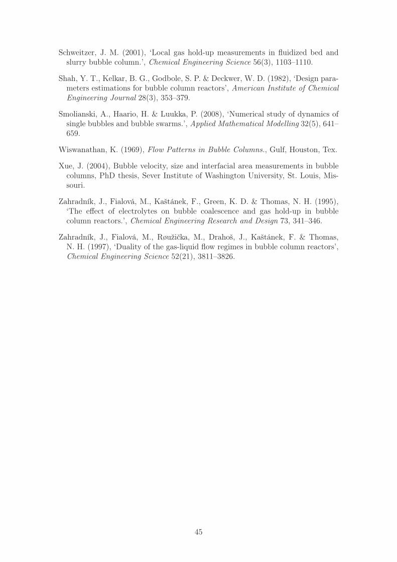
Schweitzer, J. M. (2001), ‘Local gas hold-up measurements in fluidized bed andslurry bubble column.’, Chemical Engineering Science 56(3), 1103–1110.
Shah, Y. T., Kelkar, B. G., Godbole, S. P. & Deckwer, W. D. (1982), ‘Design para-meters estimations for bubble column reactors’, American Institute of ChemicalEngineering Journal 28(3), 353–379.
Smolianski, A., Haario, H. & Luukka, P. (2008), ‘Numerical study of dynamics ofsingle bubbles and bubble swarms.’, Applied Mathematical Modelling 32(5), 641–659.
Wiswanathan, K. (1969), Flow Patterns in Bubble Columns., Gulf, Houston, Tex.
Xue, J. (2004), Bubble velocity, size and interfacial area measurements in bubblecolumns, PhD thesis, Sever Institute of Washington University, St. Louis, Mis-souri.
Zahradník, J., Fialová, M., Kaštánek, F., Green, K. D. & Thomas, N. H. (1995),‘The effect of electrolytes on bubble coalescence and gas hold-up in bubblecolumn reactors.’, Chemical Engineering Research and Design 73, 341–346.
Zahradník, J., Fialová, M., Røužička, M., Drahoš, J., Kaštánek, F. & Thomas,N. H. (1997), ‘Duality of the gas-liquid flow regimes in bubble column reactors’,Chemical Engineering Science 52(21), 3811–3826.
45

46

Chapter 3
Experimental study ofhydrodynamics and bubble size
3.1 Introduction
Bubble dispersion and bubble size are important parameters that influence theperformance of bubble column reactors. The bubble size depends on operatingconditions, global hydrodynamics and turbulence. Bubbles have a high polydis-persity, i.e. they are characterized by different sizes and velocities (Rusche & Issa2015). Only a very few papers are focused on bubble size measurements in the het-erogeneous regime, i.e. Xue (2004), Chaumat et al. (2007), McClure et al. (2015,2016, 2017). They are based on the calculation of chord distributions by multi-pointneedle probes. This technique has been validated in the case of bubbles having al-most vertical trajectories. In the case of heterogeneous regime, bubbles do not havevertical trajectories and their path becomes more chaotic as the distance from thecolumn centre increases. The measurement has then low accuracy, as stated byMcClure et al. (2013) and Xue (2004). Multi-point probes access both the bubblechord distribution and the bubble velocity. To overcome the limits of classical tech-niques, a cross-correlation (CC) technique has been recently developed to measurethe bubble size. The cross-correlation technique does not depend on the trajectoryof the bubbles, so it is well adapted to the heterogeneous regime (Raimundo 2015,Raimundo et al. 2016). In return, cross-correlation technique does not providechord distributions, but a Sauter mean diameter, that is measured with confidenceat any radial position. Chord-based measurement techniques and CC techniqueare therefore complementary.
The impact of contaminants and additives is a key point concerning bubblyflows for industrial applications, that never involve only pure fluids: complex com-positions are used. In literature, the effects of additives are not well-studied: fewexperimental well-documented works provide data on phases velocity and on bubblesize distribution (McClure et al. 2015). In aqueous solutions with alcohol, thebubbles are smaller and the transition of bubbling regimes is delayed to higher gasvelocity, due to the coalescence decrease (Keitel & Onken 1982, Guo et al. 2017)and the bubble rigidity increase (Dargar & Macchi 2006). This effect increases withalcohol molecular weight, as stated by Jamialahmadi & Miiller-Steinhagen (1992).The decrease of surface tension due to the alcohol presence is not enough to ex-plain this behaviour. Several authors (Clift et al. 1978, Kelkar et al. 1983, Lindland
47

& Terjesen 1965, Raymond & Zieminski 1971) suggest that these differences arelinked to the reduction of the bubble-rise velocity.
The sparger effect on the bubble size is another point of industrial interest, asstated by Chaumat et al. (2007) and McClure et al. (2016). The choice of thesparger gives the possibility to modify the bubble size at the column inlet. Thesparger effect is important for a height of approximately one column diameter (Polliet al. 2002).
The objective of this part of the work is to produce data that could validatebubble coalescence and breakage models. Experiments in which coalescence andbreakage change depending on the operating conditions are carried out. Demin-eralised water, tap water and demineralised water with different ethanol concen-trations are used in order to decrease bubble coalescence. Experiments are alsocarried out using two different spargers, generating very different initial bubblesizes and simulating in some cases strong bubble breakage. By considering simul-taneously additives and spargers effects, breakage and coalescence phenomena canbe decoupled. Besides the mean diameter profiles, gas fraction and liquid velocitydistributions are measured, providing a very useful and accurate set of experimentaldata. The cross-correlation technique was first presented by Raimundo (2015) andit was tested with tap water only. In this work, this technique is employed underthe presence of impurities and additives. Different radial and axial positions areconsidered.
3.2 Experimental tools
3.2.1 Gas volume fraction
The global gas volume fraction, also called gas hold-up, can be calculated by usingthe difference of liquid height before and after gas injection:
αg = 1− H0
Hf
(3.1)
where H0 is the non-aerated liquid height and Hf is the aerated liquid height.This method is not very precise due to the interface deformation at the top of
the column: a characteristic error of about 10% is associated with this technique.The local gas fraction can be obtained thanks to an optical probe. The local
gas volume fraction is calculated as the fraction of time in which the gas is detectedat the probe tip, as detailed by Raimundo (2015). A 1C conical mono-fibre opticalprobe is used in this work (Fig. 3.1).
3.2.2 Bubble size
Different methods could be considered to obtain the bubble size: optical probe,cross-correlation and endoscope.
Using an optical probe, the bubble chord can be computed by multiplying thetime of detection of a bubble and the bubble velocity. Liu et al. (1996) explainedhow chord length can be transformed into bubble size by modelling the bubblesas ellipsoidal. This model is defined starting with the horizontal radius and theshape of the bubble. Using this model, it is possible to obtain the vertical Sauter
48

Figure 3.1: Tip of a 1C mono-fibre optical probe (Cartellier & Barrau 1998).
mean diameter from the mean bubble chord, as detailed by Raimundo (2015). Thistechnique is valid in the case of bubbles having almost vertical trajectories. In thecase of heterogeneous flow regime, bubbles trajectories are not vertical, causinglow accuracy, as stated by McClure et al. (2013). This work is focused on theheterogeneous flow regime and then the optical probe technique cannot be used.
An endoscope could be adapted to high gas volume fraction flows. A cam-era captures a high-speed video. A Light Emitting Diode (LED) on the oppositeside provides the necessary light. In each video at least 150 bubbles should beconsidered. Each vertical and horizontal diameter is measured manually. This ap-proach is tedious and requires too much time to get the results. Consequently, itis not suitable to obtain bubble size at several operating conditions. Small bubblesare not detected due to the tool resolution. Huge bubbles are not measured as theyare bigger than the maximum size of the photos.
The mean bubble size can be obtained from the spatial cross-correlation (CC)of the signals of two optical probes (Fig. 3.2). The cross-correlation quantifiesthe similarity of two signals, analysing them simultaneously. The cross-correlationfunction is then calculated as follows (Raimundo 2015):
CC =
∫ texp0
signalA(t)signalB(t)dt
texp. (3.2)
Its value is equal to unity (maximum) if the two probes are in the same position,considering that the signals are identical. The cross-correlation decreases with thedistance between the probes. Its signal reaches an asymptotic value, that dependson the local gas volume fraction. The time-averaged horizontal diameter of thebubbles is obtained by using the CC signal, the distance between the probes andthe eccentricity of the bubbles. The two probes are placed at the same height,with a distance equal to 1 mm (Fig. 3.2). This technique can be used in the caseof heterogeneous regime and high gas volume fractions, as stated by Raimundo(2015) and Raimundo et al. (2016). It has been validated by comparing its resultswith endoscopic measurements. The error is lower than 10% for every operatingcondition.
In the case of heterogeneous regime, the bubbles are often oblate. The CCtechnique measures the horizontal diameters, by using the Sauter mean diameterof the bubbles. In the case of oblate form of the bubbles, the slope of the linearpart of the curve (θ) of the cross-correlation in function of the distance between
49

Figure 3.2: Schematic representation of the CC technique.
the probes depends only on the bubble sizes. The horizontal Sauter mean diameter(dh,32) can therefore be calculated as (Raimundo 2015):
dh,32 = − 1.46
θ 0.505 exp(0.7Ecc), (3.3)
where Ecc is the eccentricity. A constant eccentricity equal to 0.70 is considered,as this value has been obtained by Raimundo (2015) with experiments in the samerange of measurements. If the bubble shape is known, the time-averaged Sautermean diameter, also called Sauter mean diameter, can be computed, by using thetime-averaged horizontal diameter of the bubbles. The eccentricity considered inthis work is in accordance with the value calculated by using the Wellek et al.(1966) correlation for liquid drops, that depends on the surface tension and on theEötvös number.
3.2.3 Liquid velocity
The liquid velocity in bubble columns of different diameters in the heterogeneous re-gime can be obtained by using a modified Pitot tube, called a Pavlov tube (Fig. 3.3)(Forret 2003). The differential pressure between two opposite holes is measured inorder to obtain the liquid velocity. As the presence of two phases is important, Vialet al. (2003) propose to add a calibration parameter and a correction parameterthat considers the gas fraction. These measurements have an associated error ofabout 10-20%, that depends on the gas fraction.
The measured differential pressure ΔP allows the liquid velocity to be obtained:
uL,i(r, t) =
⎧⎪⎨⎪⎩√
2ΔPi
ρLforΔPi ≥ 0
−√
−2ΔPi
ρLforΔPi ≤ 0
(3.4)
50

where uL,i is the instantaneous liquid velocity and ΔPi is the instantaneous differ-ential pressure.
The average liquid velocity uL is obtained by sampling the instantaneous liquidvelocity:
uL(r) =
∑Ni=1 uL,i(r, t)
N. (3.5)
Figure 3.3: Pavlov tube (Forret 2003).
3.3 Experimental setup
Experiments are carried out in a 0.4 m diameter cylindrical bubble column (Fig. 3.4a)at atmospheric pressure for a wide range of superficial gas velocity, that varies from0.03 m/s to 0.35 m/s. The net liquid flow rate is zero. The initial liquid height(without gas) is equal to 4 diameters (H/D=4). This ratio is higher than the criticalvalue above which the gas volume fraction does not depend on the initial height,as stated by Sasaki et al. (2017). The total column height is about 8 diameters, inorder to work with very high gas volume fractions.
The techniques detailed above are used to obtain the experimental data: theglobal gas volume fraction by using the difference of liquid height, the local gasvolume fraction by using a 1C conical mono-fibre optical probe, the Sauter meandiameter by using the CC technique and the liquid velocity by using a Pavlov tubewith a sampling frequency of 400 Hz.
Different water qualities are tested in this work: demineralised water (purewater or slightly contaminated water), tap water (fully contaminated water) andsmall percentages of ethanol (0.01% and 0.05% by volume) in demineralised water.
The gas enters the column through a perforated sparger placed at the bottomof the column. Two different spargers are tested. The first sparger has 92 holesof 2 mm of diameter (Fig. 3.4b), that assures a homogeneous gas distribution.The second sparger has 7 holes of 9 mm (Fig. 3.4c), that allows analysis of theeffects of the sparger on hydrodynamics and bubble dimensions. In the secondsparger, one hole is in the sparger centre, while the other 6 holes create a hexagonat a dimensionless radial position of 0.65 (Fig. 3.4c). In the following sections,the results are mainly collected using the first sparger (92 holes of 2 mm), whilethe results collected with the second sparger (7 holes of 9 mm) are reported inSection 3.4.5.
51

Gas inlet
Gas outlet
Sparger
3.25
m
Φ 0.4 m
1 m
(a) Axial section of the bubble column
(b) Perforated sparger with 92 holes of 2 mm (c) Perforated sparger with 7 holes of 9 mm
Figure 3.4: Bubble column and spargers.
52

3.4 Experimental results
3.4.1 Gas hold-up
The global gas volume fraction is the first macroscopic property that is studied.The global gas volume fraction increases with the superficial gas velocity withdifferent slopes, depending on the operating conditions. This change of slope allowsthe homogeneous and the heterogeneous regimes to be distinguished. In Fig. 3.5and Table A.1 the measured gas hold-up is reported versus the superficial gasvelocities for demineralised water, tap water and demineralised water with differentconcentrations of ethanol. With demineralised water, the regime is homogeneous upto a superficial gas velocity of 0.05 m/s (Fig. 3.5). The global gas volume fractionincreases quickly with a linear dependence on the superficial gas velocity. After asuperficial gas velocity of 0.05 m/s, the transition regime occurs, in which the gashold-up has a low dependence on the superficial gas velocity. The hold-up curvehas a monotonic increasing trend, without any local maximum in the transitionalregime in these experiments. The heterogeneous regime begins at a superficial gasvelocity of about 0.09 m/s: at this superficial gas velocity, the gas hold-up startsto increase with a dependence that is quite linear.
0
10
20
30
40
0.00 0.10 0.20 0.30Superficial gas velocity, m/s
Glo
bal g
as v
olum
e fra
ctio
n, %
Figure 3.5: Gas hold-up versus superficial gas velocity for demineralised water(�), tap water (�), ethanol 0.01% (�) and ethanol 0.05% (�).
In the case of tap water, the gas hold-up curve shows some differences corres-ponding to the transition regime, as reported in Fig. 3.5. The behaviour at thetransition regime is influenced by the water quality used to fill the column. Tapwater results are not fully reproducible, as the water quality changes daily. Itis possible to observe that far away from the transitional regime, the trends fordemineralised water and tap water are similar.
The addition of small quantities of ethanol in water changes radically the hy-drodynamics, in particular in the case of heterogeneous regime. These differences
53

are bigger when the ethanol concentration is higher. The trends are similar underthe homogeneous regime, but the transition is delayed, as shown in Fig. 3.5. In thecase of heterogeneous regime, the differences of gas hold-up between ethanol solu-tions and demineralised water are almost constant as the superficial gas velocityincreases.
3.4.2 Local gas volume fraction
The local gas volume fraction is affected by the superficial gas velocity and theradial and axial positions. The optical probe measures correctly the local gasvolume fraction for every operating condition. The local gas volume fraction ismaximum in the column centre and minimum close to the wall, as suggested by thecorrelation of Schweitzer (2001). The gas volume fraction profile is symmetric andit can be assumed, in first approximation, as parabolic. Increasing the superficialgas velocity, the local gas fraction value becomes higher for every bubble columnposition. The effect is more important in the column centre, where the largestbubbles rise to the top. Close to the wall, the smallest bubbles are dragged downby the liquid that recirculates.
In the case of homogeneous regime, the radial profile is less pronounced. Bigbubbles appear in the centre of the column and the gas fraction radial profile has astronger concavity in the case of heterogeneous and transition regimes, as reportedin Fig. 3.6 and Table A.2.
The axial gas fraction profile in the column centre increases along the axialposition (Fig. 3.7, Table A.6 and Table A.7). More gas is trapped in the highestpart of the column. This axial effect is present under both the homogeneous andthe heterogeneous regimes. This effect may be important for industrial applica-tions: increasing the axial position, the radial gas volume fraction profile is morepronounced and can lead to strong heterogeneities in products concentrations, forinstance.
As observed with the global gas hold-up (Fig. 3.5), the effect of the tap wateron the gas volume fraction is low for both homogeneous and heterogeneous regimes(Fig. 3.6 and Table A.3). Adding few percent of ethanol, the transition is delayed:with a superficial gas velocity of 0.06 m/s, the radial gas volume fraction profileis almost flat. In the case of homogeneous regime, the local gas fraction is almostnot influenced by the presence of ethanol. In the case of heterogeneous regime, thelocal gas fraction is higher if small quantities of ethanol are present (Fig. 3.6).
In the case of heterogeneous regime, the local gas fraction increases adding asmall quantity of alcohol for every position: this discrepancy is important both forthe radial (Fig. 3.6, Table A.4 and Table A.5) and the axial position (Fig. 3.7 andTable A.7). The ethanol effect on the gas fraction is almost absent in the case ofhomogeneous regime (Table A.6).
To further study and validate the local gas fraction measurements, they arecompared with the correlation of Schweitzer (2001) (Eq. (2.3)). It is suitable forthe prediction of gas fraction profiles under the heterogeneous regime. It does notconsider an axial evolution. In accordance with the experiments of Forret (2003),this correlation considers the local gas fraction near the wall close to zero.
Considering a superficial gas velocity of 0.16 m/s, the global gas volume fraction(measured with the difference of height of the liquid into the column) is equal to
54

0
10
20
30
0 0.25 0.5 0.75 1Radial position
(a) 0.03 m/s
0
10
20
30
0 0.25 0.5 0.75 1Radial position
(b) 0.06 m/s
0
10
20
30
40
0 0.25 0.5 0.75 1Radial position
(c) 0.09 m/s
0
10
20
30
40
0 0.25 0.5 0.75 1Radial position
(d) 0.16 m/s
01020304050
0 0.25 0.5 0.75 1Radial position
(e) 0.25 m/s
01020304050
0 0.25 0.5 0.75 1Radial position
(f) 0.35 m/s
Figure 3.6: Radial gas fraction profiles at H/D=2.5 with demineralised water (�),tap water (�), ethanol 0.01% (�) and ethanol 0.05% (�) at different superficialgas velocities. Comparison with Schweitzer (2001) correlation profiles for water
(solid lines) and ethanol 0.05% (dashed lines).
55

0
5
10
15
0 1 2 3 4Axial position (H/D)
Loca
l gas
frac
tion,
%
(a) 0.03 m/s
0
10
20
30
40
0 1 2 3 4Axial position (H/D)
Loca
l gas
frac
tion,
%
(b) 0.16 m/s
Figure 3.7: Axial gas fraction profile in the centre of the column withdemineralised water (�), tap water (�), ethanol 0.01% (�) and ethanol 0.05% (�)
at different superficial gas velocities.
56
0.26. Another method to compute the mean gas fraction is to average the radiallocal gas fraction profile in a certain axial position. In order to compute thisaverage, it is necessary to assume that the fraction of gas near the wall is equal tozero, as suggested by Schweitzer (2001) and Forret (2003). In the same operatingconditions, with a H/D = 2.5, the average of the radial local gas fraction profile isequal to 0.22. This discrepancy is due to different factors: the importance of theaxial effect (Fig. 3.7), the assumption of absence of gas near the wall and the lowprecision of the gas hold-up measured with the difference of liquid height.
The correlation of Schweitzer (2001), calculating the mean gas fraction as theaverage in the axial position of interest, fits well the experimental profile in thecase of heterogeneous regime and demineralised water (Fig. 3.6). The correlationof Schweitzer (2001) cannot be used in the case of homogeneous regime: the ex-perimental radial profile is flat, while the profile obtained from this correlation isparabolic.
Under the heterogeneous regime, the correlation of Schweitzer (2001) is suitablealso in the case of tap water and alcohol addition: the mean gas fraction changes,but a correct radial profile is obtained, as reported in Fig. 3.6.
The results of this work are qualitatively compared with the experimental res-ults of McClure et al. (2016). McClure et al. (2016) use ‘tree’ type spargers, locatedat a height of 0.135 m. The radial profiles with this sparger have an M-shape ifa symmetric sparger is used, as shown in Fig. 3.8. A perforated plate injects gashomogeneously, while a ‘tree’ type sparger cannot. The different type of spar-ger cause the experimental data differences between this work and McClure et al.(2016). For different operating conditions, the sparger choice can significantly in-fluence the global hydrodynamics.
0
10
20
30
0 0.25 0.5 0.75 1
Loca
l gas
frac
tion,
%
Radial position
Figure 3.8: Radial gas fraction profiles at H/D=2.5 with demineralised (�) andtap water (�) versus the experimental data of McClure et al. (2016) (+).
57

3.4.3 Axial liquid velocity
The mean radial profile of axial liquid velocity depends on global hydrodynamicsand on bubbles recirculation, as observed by Krishna et al. (2000b). Its radialprofile has a quadratic shape in the case of heterogeneous regime, with a strongliquid recirculation, that goes up in the column centre and goes down next to thewall, as reported in Fig. 3.9 and Table A.8. The radial profile is more pronouncedin the case of heterogeneous regime and it is almost flat under the homogeneousregime. For a superficial gas velocity of 0.06 m/s, using demineralised water, thetransition regime appears: the radial profile is quadratic with a weak concavity,i.e. the profile is halfway between the homogeneous and the heterogeneous regime.These results are in accordance with gas hold-up and local gas volume fractionprofiles.
-1
-0.5
0
0.5
1
0 0.25 0.5 0.75 1
Axi
al li
quid
vel
ocity
, m/s
Radial position
Figure 3.9: Radial profile of axial liquid velocity at H/D=2.5 with demineralisedwater for different superficial gas velocities: 0.03 m/s (�), 0.06 m/s (�), 0.09 m/s
(×) and 0.16 m/s (�).
In the case of heterogeneous regime, the mean axial liquid velocity profile andthe recirculation does not seem to be influenced by the presence of contaminantsin the water (Fig. 3.10 and Table A.9). The velocity profile depends on the verticalposition close to the sparger, while the dependence is negligible in the case ofH/D>1.
These experimental data are compared with the correlation of Forret (2003)(Eq. (2.10)) (Fig. 3.10). This correlation allows the radial profile of the liquid axialvelocity to be defined if the liquid velocity at the column centre is known. Thisequation can be used in presence of contaminants and additives.
The experimental liquid velocity in the centre of the column is then comparedwith the correlation proposed by Miyauchi & Shyu (1970) (Eq. (2.11)), that canbe used for many operating conditions under the heterogeneous regime. This cor-relation can also be used for scale-up purposes, but it cannot be used in presence
58

-1
-0.5
0
0.5
1
0 0.25 0.5 0.75 1
Axi
al li
quid
vel
ocity
, m/s
Radial position
Figure 3.10: Radial profile of axial liquid velocity for a superficial gas velocity of0.16 m/s at H/D=2.5 for demineralised water (�), tap water (�) and ethanol
0.05% (�); radial profiles are compared with the correlations proposed byMiyauchi & Shyu (1970) and Forret (2003) (solid line).
of contaminants and additives. It slightly underestimates the liquid velocity in thecolumn centre also without additives.
3.4.4 Bubble size
The Sauter mean diameter is obtained from the CC measurements for differentwater qualities, for a wide range of superficial gas velocity, from 0.03 m/s to 0.35m/s. These results are given on Fig. 3.11 and reported in Table A.10, Table A.11,Table A.12 and Table A.13.
The radial profile of the Sauter mean diameter is symmetrical with a maximumin the centre. In the case of homogeneous regime, the profile is flatter. When thesuperficial gas velocity increases, the concavity grows. In the case of heterogeneousregime, big bubbles are formed. These bubbles they rise in the column centre, whilesmall bubbles are dragged down by the liquid recirculation near the wall. Radialprofiles of gas volume fraction, liquid velocity and bubble size are interconnectedand consistent.
The axial evolution of the Sauter mean diameter in the column centre is reportedin Fig. 3.12, in Table A.14 and in in Table A.15. The Sauter mean diameter slightlydecreases for both media close to the sparger. Close to the bottom, the bubble sizeprofile is not developed and it needs about 0.5 m to reach a stable radial profile;above this height, the bubble size grows along the axial position. (Fig. 3.12). Thisincrease can be partially due to the decrease of pressure along the column. Theideal gas law can be used to obtain a first approximation valuation: this effect isless than 5%, while experimentally the increase is more than 20%. It means thatother factors are involved. This phenomenon is still difficult to explain. A partial
59

02468
10
0 0.25 0.5 0.75 1Radial position
(a) 0.03 m/s
02468
10
0 0.25 0.5 0.75 1Radial position
(b) 0.06 m/s
02468
10
0 0.25 0.5 0.75 1Radial position
(c) 0.09 m/s
02468
10
0 0.25 0.5 0.75 1Radial position
(d) 0.16 m/s
02468
10
0 0.25 0.5 0.75 1Radial position
(e) 0.25 m/s
02468
10
0 0.25 0.5 0.75 1Radial position
(f) 0.35 m/s
Figure 3.11: Sauter mean diameter profiles at H/D=2.5 with demineralised water(�), tap water (�), ethanol 0.01% (�) and ethanol 0.05% (�) at different
superficial gas velocities.
60

explanation could be the higher concavity of the radial profiles along the axialposition, that causes an increase of the parabola maximum. The main phenomenonthat should cause the axial increase should be the bubble coalescence.
0
2
4
6
8
10
0 1 2 3 4 5
Saut
er m
ean
diam
eter
, mm
Axial position (H/D)Figure 3.12: Axial Sauter mean diameter profile in the centre of the column for a
superficial gas velocity of 0.16 m/s (heterogeneous regime) with demineralisedwater (�) and ethanol 0.05% (�).
The Sauter mean diameter in demineralised water is higher than in tap water(Fig. 3.11) for every operating condition: water contamination has an importanteffect on the bubble size. Adding ethanol, the Sauter mean diameter becomeslower in comparison with the case of demineralised water, but increases with thesuperficial gas velocity. Adding ethanol, the radial profile is almost flat both for 0.03m/s and for 0.06 m/s (Fig. 3.11), confirming the delay in entering the transitionregime, as suggested by global and local gas volume fraction. The bubble size islower if the concentration of ethanol is higher. The ethanol effect is consistentwith the results of McClure et al. (2015), adding 2-propanol into water. Smallquantity of ethanol and presence of impurities in tap water decrease coalescence;as a consequence, the Sauter mean diameter is lower.
The surface tension difference is too small to have an effect: at 17 ◦C, with anethanol concentration of 0.05%, it goes from 0.07335 N/m to 0.07325 N/m. Thesurface tension decrease is not enough to explain the differences: a small variationof temperature would have a stronger effect than the presence of ethanol. It meansthat other phenomena are at stake. (Kelkar et al. 1983) suggest that the differencesare caused by the bubble-rise velocity reduction. This explanation is reasonablefor the homogeneous regime, where the bubbles go up vertically and the bubblevelocity tends to the terminal velocity. As suggested by several authors (Camarasaet al. 1999, Zahradník et al. 1995, 1997), under the heterogeneous regime, themacro-scale turbulence effect eclipses the others. The effect on the gas fractioncan be entirely explained by the delay in entering the transitional regime (Krishnaet al. 2000a). The homogeneous regime is larger and the gas hold-up at transition
61

in presence of alcohol can be estimated by using the correlation proposed by Reillyet al. (1994).
As presented in Fig. 3.11 for a superficial gas velocity of 0.06 m/s, lower coales-cence causes a transition delay: a lower coalescence rate causes smaller bubbles,resulting in a higher gas hold-up into the column. Bigger bubbles feel a higherbuoyancy force (in comparison with the drag force) and they rise more quickly. Asbig bubbles rise quickly in the column centre, the transition from the homogen-eous regime to the transition regime and to the heterogeneous regime is affected.By using an endoscope, Raimundo (2015) measured the bubble size distributions,observing that they are wide, but still unimodal or bimodal with a predominantpeak. The biggest bubbles are in the column centre.
The principal effect of alcohol is to modify the surface mobility of the bubbles,as stated by Najafi et al. (2007). In the case of pure systems, the bubble interfaceis mobile. In this case, the liquid film between the approaching bubbles drainsout quickly. Alcohol forms a monolayer at the interface; that causes an additionalresistance to the liquid film motion (Jamialahmadi & Miiller-Steinhagen 1992).This additional resistance increases the liquid film drainage time. Consequently, theoverall coalescence rate decreases. Takahashi (2005) stated that another importantaspect is linked to the effect of alcohol on the zeta-potential of the bubbles.
3.4.5 Effect of the sparger on demineralized water systems
A sparger with 92 holes of 2 mm in diameter (Fig. 3.4b) ensures a homogeneous gasdistribution and a generation of small bubbles. The bubble distribution is optimal.Dead zones in the bubble column are absent.
A sparger with 7 holes of 9 mm is used to form bigger bubbles and to enhancebubble breakage close to the bottom of the column. Gas injection with this spargeris completely different: the gas is injected heterogeneously in a small fraction of thecolumn section and is then concentrated close to the holes. In correspondence of thecolumn centre, where the data is collected, the new sparger has a hole (Fig. 3.4c).
The axial gas fraction profiles obtained with the two spargers are comparedin Fig. 3.13 (Table A.16, Table A.17 and Table A.18). More gas accumulatesnear the sparger in the column centre if the 7-holes sparger is used, in the case ofheterogeneous regime. The sparger effect is important for every column positionin the case of homogeneous regime and it determines the gas volume fraction inthe entire column: using the 7-holes sparger, the gas fraction is lower than whenusing the 92-holes sparger for every axial position. Under the heterogenous regime,the sparger effect is important in the lowest part on the column, while its effect isalmost null above a certain height.
Close to the bottom of the column, by using the 92-holes sparger, the radial pro-file of the gas fraction is almost flat (Fig. 3.14) contrary to the results obtained withthe 7-holes sparger: a strong bubble accumulation appears above the holes, whilethe gas concentration is low in the other radial positions. As shown in Fig. 3.14(Table A.19 and Table A.20), the gas volume fraction with the two spargers isapproximately identical under the heterogeneous regime above an axial position of0.5 m.
The initial dimension of the bubbles is strongly influenced by the sparger choice,with the formation of very large bubbles (more than 20 mm) close to the bottom
62
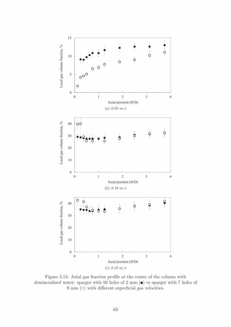
0
5
10
15
0 1 2 3 4
Loca
l gas
vol
ume
fract
ion,
%
Axial position (H/D)
(a) 0.03 m/s
0
10
20
30
40
0 1 2 3 4
Loca
l gas
vol
ume
fract
ion,
%
Axial position (H/D)
(b) 0.16 m/s
0
10
20
30
40
0 1 2 3 4
Loca
l gas
vol
ume
fract
ion,
%
Axial position (H/D)
(c) 0.25 m/s
Figure 3.13: Axial gas fraction profile at the centre of the column withdemineralised water: sparger with 92 holes of 2 mm (�) vs sparger with 7 holes of
9 mm (�) with different superficial gas velocities.
63

0
5
10
15
0 0.25 0.5 0.75 1
Radial position
Loca
l gas
frac
tion,
%
(a) 0.03 m/s
0
10
20
30
40
0 0.25 0.5 0.75 1
Radial position
Loca
l gas
frac
tion,
%
(b) 0.16 m/s
Figure 3.14: Radial gas fraction profile at different axial positions withdemineralised water: sparger with 92 holes of 2 mm (H/D=2.5 (�) and H/D=0.25
(�) vs sparger with 7 holes of 9 mm (H/D=2.5 (�) and H/D=0.25 (�)) withdifferent superficial gas velocities.
64
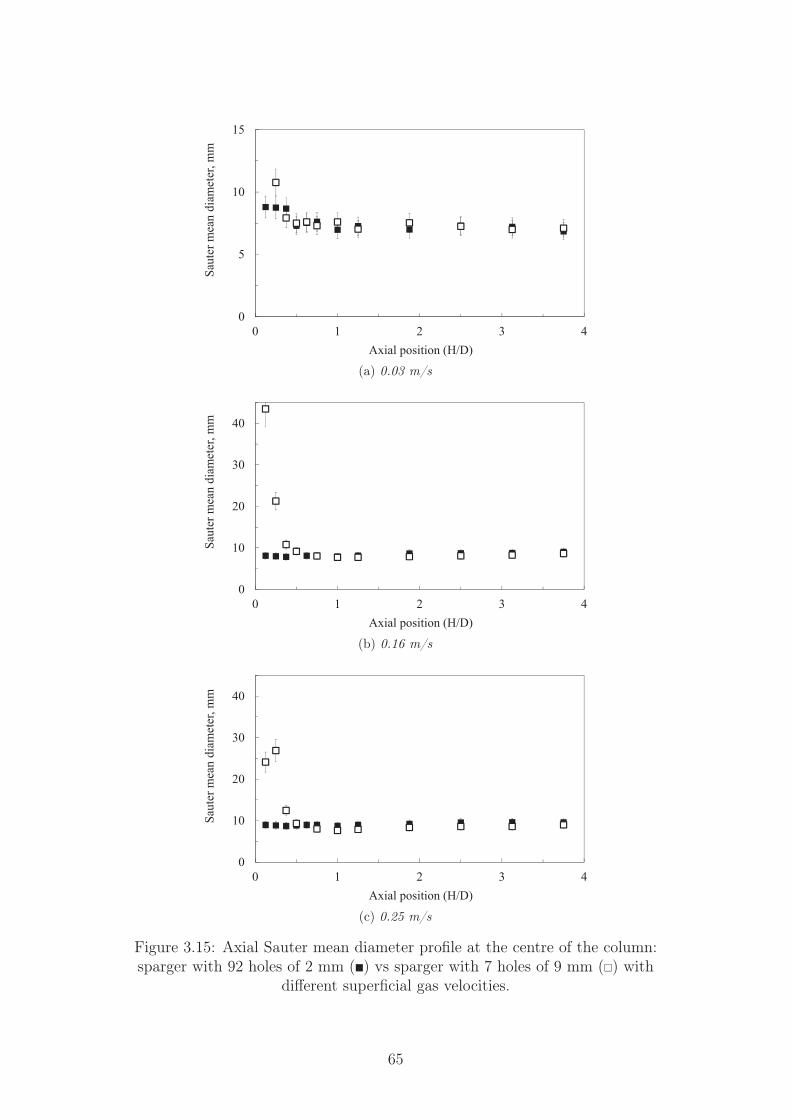
0
5
10
15
0 1 2 3 4
Saut
er m
ean
diam
eter
, mm
Axial position (H/D)
(a) 0.03 m/s
0
10
20
30
40
0 1 2 3 4
Saut
er m
ean
diam
eter
, mm
Axial position (H/D)
(b) 0.16 m/s
0
10
20
30
40
0 1 2 3 4
Saut
er m
ean
diam
eter
, mm
Axial position (H/D)
(c) 0.25 m/s
Figure 3.15: Axial Sauter mean diameter profile at the centre of the column:sparger with 92 holes of 2 mm (�) vs sparger with 7 holes of 9 mm (�) with
different superficial gas velocities.
65

0
5
10
15
0 0.25 0.5 0.75 1
Radial position
Saut
er m
ean
diam
eter
, mm
(a) 0.03 m/s
0
5
10
15
20
0 0.25 0.5 0.75 1
Radial position
Saut
er m
ean
diam
eter
, mm
(b) 0.16 m/s
Figure 3.16: Radial Sauter mean diameter profile at different axial positions withdemineralised water: sparger with 92 holes of 2 mm (H/D=2.5 (�) and H/D=0.25
(�)) vs sparger with 7 holes of 9 mm (H/D=2.5 (�) and H/D=0.25 (�)) withdifferent superficial gas velocities.
66

using the 7-holes sparger in correspondence of the holes, as shown in Fig. 3.15(Table A.21, Table A.22 and Table A.23). The Sauter mean diameter decreasesrapidly along the axial position and after some centimetres, the bubble size is almostidentical to the case of 92-holes sparger (Fig. 3.16, Table A.24 and Table A.25).Under the heterogeneous regime, the sparger has a weak effect both on gas fractionand on Sauter mean diameter above an axial position of 1 m. In the case ofheterogeneous regime, the initial bubble size does not influence the final bubblesize. This effect cannot be neglected in the lowest part of the column. Close tothe bottom, the radial profile of the Sauter mean diameter is flat with the 92-holessparger, while it is irregular with the other sparger, as detailed in Fig. 3.16. Theirregularity of this profile is partially due to the creation of random preferentialpaths of the bubbles. The sparger effect on the bubble size is only important inthe region close to the bottom, where the Sauter mean diameter is very high. Ifthe Sauter mean diameter is very high, bubble breakage is stronger than bubblecoalescence. Bubble breakage is the main phenomenon and bubble coalescence canbe neglected.
3.4.6 Effect of sparger for different media
The effects of additives and sparger design are coupled. The sparger effect is thesame both with demineralised water and with ethanol addition under the het-erogeneous regime: more gas accumulates near the sparger in the column centre.Under the heterogeneous regime, the sparger effect becomes null above 1 m: thegas fraction is not influenced by the sparger above this height, both with demin-eralised water and in presence of ethanol (Fig. 3.17 and Table A.17)). This aspectis reasonably consistent with the conclusion of Polli et al. (2002), stating thatthe sparger effect is important up to a distance of the order of magnitude of thediameter of the column. Under the heterogeneous regime, alcohol addition has arelatively low effect close to the sparger, but it affects the gas fraction in the entirebubble column. Under the homogeneous regime, the ethanol addition has a lowereffect than under the heterogeneous regime (Fig. 3.17), while the sparger choiceinfluences the gas fraction in the entire column (Table A.16).
As shown in Fig. 3.18, the final dimension of the bubbles is almost not influencedby the initial bubble size under the heterogeneous regime, while the alcohol presenceis very important (Table A.21, Table A.22 and Table A.23). The alcohol presencealmost does not influence the rate of bubble size decrease. The alcohol effect isimportant only when the bubble size reaches equilibrium. In the lower part of thecolumn with the 7-holes sparger, when the bubbles are huge, bubble breakage canbe considered as the main phenomenon and bubble coalescence is negligible. Itallows decoupling bubble breakage and bubble coalescence. A priori, the alcoholpresence can infer coalescence and break-up rates. Experimental data show that thepresence of alcohol almost does not modify the rate with which bubbles coming outof the sparger reduce their size, but on the contrary it affects the final equilibriumsize. From these observations, it is possible to state that the alcohol does notchange significantly the break-up rate, but it reduces the coalescence rate. Themain alcohol effect is on the bubble surface mobility and then it is reasonable thatthe coalescence rate, that depends on the bubble surface mobility, is influenced inturn by the presence of alcohol.
67

0
5
10
15
0 1 2 3 4
Loca
l gas
vol
ume
fract
ion,
%
Axial position (H/D)
(a) 0.03 m/s
0
10
20
30
40
50
0 1 2 3 4
Loca
l gas
vol
ume
fract
ion,
%
Axial position (H/D)
(b) 0.16 m/s
0
10
20
30
40
50
60
0 1 2 3 4
Loca
l gas
vol
ume
fract
ion,
%
Axial position (H/D)
(c) 0.25 m/s
Figure 3.17: Axial gas fraction profile at the centre of the column: sparger with92 holes of 2 mm (with demineralised water (�) and ethanol 0.05% (�)) vs
sparger with 7 holes of 9 mm (with demineralised water (�) and ethanol 0.05%(�)) with different superficial gas velocities.
68

0
5
10
15
0 1 2 3 4
Saut
er m
ean
diam
eter
, mm
Axial position (H/D)
(a) 0.03 m/s
0
10
20
30
40
0 1 2 3 4
Saut
er m
ean
diam
eter
, mm
Axial position (H/D)
(b) 0.16 m/s
0
10
20
30
40
0 1 2 3 4
Saut
er m
ean
diam
eter
, mm
Axial position (H/D)
(c) 0.25 m/s
Figure 3.18: Axial Sauter mean diameter profile at the centre of the column:sparger with 92 holes of 2 mm (with demineralised water (�) and ethanol 0.05%(�)) vs sparger with 7 holes of 9 mm (with demineralised water (�) and ethanol
0.05% (�)) with different superficial gas velocities.
69

3.5 Conclusions and perspectivesThe goal of this experimental part is to study hydrodynamics and bubble size inbubble columns under the heterogeneous regime, with the objective of highlightingand studying the breakage and coalescence phenomena.
The use of different quality of water and the addition of small quantities ofethanol is used to control coalescence. Bubble sizes in fully contaminated systemsare significantly lower than in pure or slightly contaminated water. The presenceof small percentages of ethanol into demineralised water delays the transition re-gime and heterogeneous regime occurs later. Water contamination increases thegas volume fraction and decreases the bubble dimension in the case of heterogen-eous regime. Tap water causes similar consequences. Surface tension variationsare not enough to explain these differences. The alcohol presence modifies thesurface mobility of the bubbles. If the surface mobility is lower the coalescencerate decreases and then the bubbles are smaller. Further investigations concern-ing interface physical properties are necessary to understand how alcohol presenceinhibits coalescence.
The sparger choice strongly influences gas volume fraction and bubble size inthe lowest part of the column, close to the bottom. By using a perforated spargerwith big holes, there is an accumulation of big bubbles close to the bottom, in cor-respondence of the holes. In this zone, bubble breakage is the main phenomenon.It allows identifying some configurations in which bubble generation and breakageare the only governing phenomena. The use of both different spargers and alco-hol addition allows stating that bubble breakage is almost not influenced by thepresence of alcohol: alcohol effect changes the surface mobility and then affectsmainly the bubble coalescence. Coalescence models ought to consider the impactof additives, that drastically change the coalescence rate without modifying thephysical properties involved.
Bubble size distributions (BSD) would be interesting to get, but unfortunatelythe CC technique is not able to calculate the BSD: A possible perspective couldbe to couple a classical optical probe for BSD measurements with a CC probe forthe Sauter mean diameter. It could allow rescaling the BSD, that is not preciselymeasured with a classical optical probe in the case of heterogeneous regime.
70

Bibliography
Camarasa, E., Vial, C., Poncin, S., Wild, G., Midoux, N. & Bouillard, J. (1999),‘Influence of coalescence behaviour of the liquid and of gas sparging on hydro-dynamics and bubble characteristics in a bubble column.’, Chemical Engineeringand Processing 38, 329–344.
Cartellier, A. & Barrau, E. (1998), ‘Monofiber optical probes for gas detection andgas velocity measurements: conical probes.’, International Journal of MultiphaseFlow 24(8), 1265–1294.
Chaumat, H., Billet, A. & Delmas, H. (2007), ‘Hydrodynamics and mass transfer inbubble column: Influence of liquid phase surface tension.’, Chemical EngineeringScience 62, 7378–7390.
Clift, R., Grace, J. R. & Weber, M. E. (1978), Bubbles, Drops, and Particles.,Academic Press, New York, New York.
Dargar, P. & Macchi, A. (2006), ‘Effect of surface-active agents on the phaseholdups of three-phase fluidized beds.’, Chemical Engineering and Processing45, 764–772.
Forret, A. (2003), Hydrodynamics scale-up of slurry bubble columns., PhD thesis,Université Claude Bernard Lyon 1 - IFPEN, Lyon.
Guo, K., Wang, T., Liu, Y. & Wang, J. (2017), ‘CFD-PBM simulations of a bubblecolumn with different liquid properties’, Chemical Engineering Journal 329(Sup-plement C), 116–127.
Jamialahmadi, M. & Miiller-Steinhagen, H. (1992), ‘Inhibition of bubble coales-cence by solutes in air/water dispersions.’, Chemical Engineering Journal 50, 47–56.
Keitel, G. & Onken, U. (1982), ‘Inhibition of bubble coalescence by solutes inair/water dispersions.’, Chemical Engineering Science 37, 1635–1638.
Kelkar, B. G., Godbole, S. P., Honath, M. F. & Shah, Y. T. (1983), ‘Effect ofaddition of alcohols on gas holdup and backmixing in bubble columns.’, AmericanInstitute of Chemical Engineering Journal 29, 361–369.
Krishna, R., Dreher, A. J. & Urseanu, M. I. (2000a), ‘Influence of alcohol ad-dition on gas hold-up in bubble columns: Development of a scale up model.’,International Communications in Heat and Mass Transfer 27(4), 465–472.
Krishna, R., Urseanu, M. I., Van Baten, J. & Ellenberger, J. (2000b), ‘Liquidphase dispersion in bubble columns operating in the churn-turbulent flow regime’,Chemical Engineering Journal 78(1), 43 – 51.
Lindland, K. P. & Terjesen, S. G. (1965), ‘The effect of a surface-active agent onmass transfer in falling drop extraction.’, Chemical Engineering Science 5(1), 1–12.
71

Liu, W., Clark, N. N. & Karamavruc, A. I. (1996), ‘General method for the trans-formation of chord-length data to a local bubble-size distribution.’, AmericanInstitute of Chemical Engineering Journal 42(10), 2713–2720.
McClure, D. D., Kavanagh, J. M., Fletcher, D. F. & Barton, G. W. (2013), ‘De-velopment of a CFD model of bubble column bioreactors: Part one - a detailedexperimental study’, Chemical Engineering & Technology 36(12), 2065–2070.
McClure, D. D., Kavanagh, J. M., Fletcher, D. F. & Barton, G. W. (2017), ‘Exper-imental investigation into the drag volume fraction correction term for gas-liquidbubbly flows’, Chemical Engineering Science 170, 91–97.
McClure, D. D., Norris, H., Kavanagh, J. M., Fletcher, D. F. & Barton, G. W.(2015), ‘Towards a CFD model of bubble columns containing significant surfact-ant levels.’, Chemical Engineering Science 127, 189–201.
McClure, D. D., Wang, C., Kavanagh, J. M., Fletcher, D. F. & Barton, G. W.(2016), ‘Experimental investigation into the impact of sparger design on bubblecolumns at high superficial velocities.’, Chemical Engineering Research andDesign 106, 205–213.
Miyauchi, T. & Shyu, C. N. (1970), ‘Flow of fluid in gas-bubble columns’, Chemicalengineering 34(9), 958–964.
Najafi, A. S., Drelich, J., Yeung, A., Xu, Z. & Masliyah, J. (2007), ‘A novel methodof measuring electrophoretic mobility of gas bubbles.’, Journal of Colloid andInterface Science 308(2), 344–350.
Polli, M., Di Stanislao, M., Bagatin, R., Abu Bakr, E. & Masi, M. (2002), ‘Bubblesize distribution in the sparger region of bubble columns’, Chemical EngineeringScience 57(1), 197–205.
Raimundo, P. M. (2015), Analysis and modelization of local hydrodynamics inbubble columns., PhD thesis, Université Grenoble Alpes.
Raimundo, P. M., Cartellier, A., Beneventi, D., Forret, A. & Augier, F. (2016),‘A new technique for in-situ measurements of bubble characteristics in bubblecolumns operated in the heterogeneous regime’, Chemical Engineering Science155, 504 – 523.
Raymond, D. R. & Zieminski, S. A. (1971), ‘Mass transfer and drag coefficientsof bubbles rising in dilute aqueous solutions.’, American Institute of ChemicalEngineering Journal 17(1), 57–65.
Reilly, I. G., Scott, D. S., De Bruijn, T. J. W. & MacIntyre, D. (1994), ‘The role ofgas phase momentum in determining gas hold-up and hydrodynamic flow regimesin bubble column operations.’, The Canadian Journal of Chemical Engineering72, 3–12.
Rusche, H. & Issa, R. (2015), Simulation of a reactive gas-liquid system withquadrature-based moments method., in ‘Eleventh International Conference onComputational Fluid Dynamics in the Minerals and Process Industries’, Mel-bourne, Victoria, Australia.
72

Sasaki, S., Uchida, K., Hayashi, K. & Tomiyama, A. (2017), ‘Effects of columndiameter and liquid height on gas holdup in air-water bubble columns.’, Experi-mental Thermal and Fluid Science 82, 359–366.
Schweitzer, J. M. (2001), ‘Local gas hold-up measurements in fluidized bed andslurry bubble column.’, Chemical Engineering Science 56(3), 1103–1110.
Takahashi, M. (2005), ‘ζ potential of microbubbles in aqueous solutions: Elec-trical properties of the gas-water interface.’, The Canadian Journal of ChemicalEngineering 109(46), 21858–21864.
Vial, C., Bendjaballah-Lalaoui, N., Poncin, S., Wild, G. & Midoux, N. (2003),‘Comparison, combination and validation of measuring techniques for local flowand turbulence analysis in bubble columns and airlift reactors.’, The CanadianJournal of Chemical Engineering 81(3-4), 749–755.
Wellek, R. M., Agrawal, A. K. & Skelland, A. H. P. (1966), ‘Shape of liquid dropsmoving in liquid media’, American Institute of Chemical Engineering Journal12(5), 854–862.
Xue, J. (2004), Bubble velocity, size and interfacial area measurements in bubblecolumns., PhD thesis, Sever Institute of Washington University.
Zahradník, J., Fialová, M., Kaštánek, F., Green, K. D. & Thomas, N. H. (1995),‘The effect of electrolytes on bubble coalescence and gas hold-up in bubblecolumn reactors.’, Chemical Engineering Research and Design 73, 341–346.
Zahradník, J., Fialová, M., Røužička, M., Drahoš, J., Kaštánek, F. & Thomas,N. H. (1997), ‘Duality of the gas-liquid flow regimes in bubble column reactors’,Chemical Engineering Science 52(21), 3811–3826.
73

74
Chapter 4
CFD simulations: hydrodynamicsand mixing
4.1 Introduction
Bubble column reactors require effective mass, momentum and energy transfersbetween the liquid and the gaseous phases. Although bubble column reactorsappear simple, their modelling is difficult. Phase velocities, gas volume fraction,bubble size, flow pattern and turbulence depend on the operating conditions and onthe bubble column design and they are linked in a complex way. Moreover, in thecase of heterogeneous churn-turbulent flow regime, local profiles of the propertiesof interest depend strongly on the radial position. Models for the simulation ofbubble column reactors suitable for both homogeneous and heterogeneous regimestill need to be developed.
CFD simulations are a promising tool for the study of large bubble columnsin a wide range of operating conditions. A common choice is to model these sys-tems with Reynolds-averaged Navier-Stokes (RANS) equations and by using theEulerian-Eulerian multiphase model, describing the two phases as inter-penetratingcontinua, as stated by Zhang (2007), Vaidheeswaran & Lopez de Bertodano (2017).The interactions between the continuous and the disperse phases must be accuratelymodelled (Jakobsen et al. 2005). These interactions are dominated by different in-terfacial forces (McClure et al. 2013, Hlawitschka et al. 2017) and the drag force isthe most important. In the case of high gas volume fractions, the distance betweenbubbles is small and the bubble boundary layers interact, modifying the drag force.This phenomenon can be considered by adding a swarm factor. In the literature,several drag force correlations and swarm factors have been proposed. Differentswarm factors are suitable for low gas volume fractions, while few correlations havebeen proposed for high gas volume fractions (e.g. McClure et al. (2017b)). Thesecorrelations are often empirical or obtained through Direct Numerical Simulations.They are usually based on experiments carried out under the homogeneous regimeand then they have a narrow validity range.
Drag law expressions, including swarm factor, can be studied and validatedthanks to the experimental data of (Raimundo 2015) and the experiments detailedin Chapter 3 and in Gemello et al. (2018) for a wide range of superficial gas ve-locities, going from 0.03 m/s to 0.35 m/s and at different scales. Experimentalgas hold-up, local gas volume fraction and axial liquid velocity are compared with
75

CFD results. The bubble size cannot be compared with the CFD simulations atthis stage: classical CFD simulations consider a fixed bubble size as input para-meter. The population balance model proposed in Chapter 5 will allow overcomingthis limit. In the first part of this chapter, different drag laws and swarm factorsare tested, with a view to obtaining a swarm factor suitable for several operatingconditions.
The choice of the turbulence model is another important point for obtainingreasonable CFD results. Classical models of turbulence are based on the Boussinesq(1897) hypothesis. The choice of the turbulence model has a strong impact on theturbulent mixing, that is a key property for bubble column reactors. In the secondpart of this chapter, four different turbulence models, already usable in ANSYSFluent, are tested: standard k-ε, realizable k-ε, RNG k-ε and k-ω model.
Bubble contribution to mixing is considered in this work. It affects strongly themixing, as detailed by Alméras et al. (2016) for the homogeneous regime. With thismethod, shear-induced turbulence (SIT) and bubble contributions are attributableto similar diffusive properties. Alméras et al. (2015) stated that the bubbles havean influence on the dispersion of a passive scalar in the case of bubbly flows,characterizing the contribution of bubble wake interactions by adding a bubble-induced diffusivity to the scalar transport equations. Mixing due to the bubblecontribution is studied in the last part of this chapter.
Turbulence due to energy transfer from gas to liquid could be included in aRANS model with different techniques, as detailed by Joshi (2001). Pfleger &Becker (2001), Yao & Morel (2004) and Rzehak & Krepper (2013) suggest addingdirectly the source terms in the turbulence properties transport equations, as poin-ted out by Fletcher et al. (2017) and McClure et al. (2017a) for predicting mixing.However, this contribution needs clarifications, in particular for bubble columns athigh gas volume fractions. Sato & Sekoguchi (1975) stated that only a fractionof this contribution forms a source term for the turbulence kinetic energy. Turbu-lence due to energy transfer from gas to liquid is neglected in this chapter, withoutadding source terms in k and ε (or ω) equations.
4.2 Modelling of bubble columnsFluid flows are defined by the continuity equation, that represents the local con-servation of mass, and by the Navier-Stokes equation, that characterizes the localconservation of momentum (Bird et al. 2007):
∂ρ
∂t+∇ρu = 0, (4.1)
∂ (ρu)
∂t+∇ · (ρuu) +∇p = ∇ · T + g (4.2)
where T is the viscous stress tensor and g is the body forces vector. For a Newto-nian fluid, T is equal to:
T = μ
[∇u+ (∇u)T − 2
3∇ · uI
](4.3)
where I is the identity matrix.
76
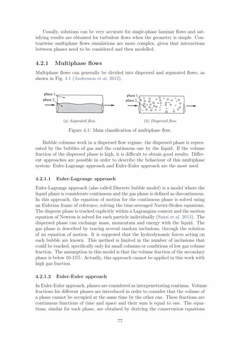
Usually, solutions can be very accurate for single-phase laminar flows and sat-isfying results are obtained for turbulent flows when the geometry is simple. Con-trariwise multiphase flows simulations are more complex, given that interactionsbetween phases need to be considered and then modelled.
4.2.1 Multiphase flows
Multiphase flows can generally be divided into dispersed and separated flows, asshown in Fig. 4.1 (Andersson et al. 2012).
(a) Separated flow. (b) Dispersed flow.
Figure 4.1: Main classification of multiphase flow.
Bubble columns work in a dispersed flow regime: the dispersed phase is repres-ented by the bubbles of gas and the continuous one by the liquid. If the volumefraction of the dispersed phase is high, it is difficult to obtain good results. Differ-ent approaches are possible in order to describe the behaviour of this multiphasesystem: Euler-Lagrange approach and Euler-Euler approach are the most used.
4.2.1.1 Euler-Lagrange approach
Euler-Lagrange approach (also called Discrete bubble model) is a model where theliquid phase is considerate continuous and the gas phase is defined as discontinuous.In this approach, the equation of motion for the continuous phase is solved usingan Eulerian frame of reference, solving the time-averaged Navier-Stokes equations.The disperse phase is tracked explicitly within a Lagrangian context and the motionequation of Newton is solved for each particle individually (Suzzi et al. 2013). Thedispersed phase can exchange mass, momentum and energy with the liquid. Thegas phase is described by tracing several random inclusions, through the solutionof an equation of motion. It is supposed that the hydrodynamic forces acting oneach bubble are known. This method is limited in the number of inclusions thatcould be tracked, specifically only for small columns or conditions of low gas volumefraction. The assumption in this model is that the volume fraction of the secondaryphase is below 10-15%. Actually, this approach cannot be applied in this work withhigh gas fraction.
4.2.1.2 Euler-Euler approach
In Euler-Euler approach, phases are considered as interpenetrating continua. Volumefractions for different phases are introduced in order to consider that the volume ofa phase cannot be occupied at the same time by the other one. These fractions arecontinuous functions of time and space and their sum is equal to one. The equa-tions, similar for each phase, are obtained by deriving the conservation equations
77

for each phase. The Euler-Euler approach presents three models of multiphase flow:volume of fluid (VOF), mixture model and Eulerian model.The Eulerian model isdescribed and used in this work.
Using the Eulerian multiphase model, a single pressure is shared by all phases;momentum and continuity equations are solved instead for each phase. With theEulerian multiphase model, the number of secondary phases is limited only bymemory requirements and convergence behaviour. Any number of secondary phasescan be modelled, provided that sufficient memory is available. For complex mul-tiphase flows, it is possible that each solution is limited by convergence behaviour.The volume of phase q, Vq, is defined by:
Vq =
∫V
αqdV (4.4)
where:n∑
q=1
αq = 1. (4.5)
The continuity equation for phase q is:
∂ (αqρq)
∂t+∇ · (αqρquq) =
n∑p=1
(mpq − mqp) (4.6)
where uq is the velocity of phase q and mpq characterizes the mass transfer fromthe phase p to the phase q.
The momentum balance for phase q is:
∂ (αqρquq)
∂t+∇ · (αqρququq) =
= −αq∇p+∇ · (αqτ q) + αqρqg +n∑
p=1
(mpqupq − mqpuqp) + F (4.7)
where τ q is stress-strain tensor for the phase q.If phase p mass is transferred to phase q (mpq > 0), upq = up; if phase q mass
is transferred to phase p (i.e. mpq < 0), upq = uq. If mqp > 0 then uqp = uq, ifmqp < 0 then uqp = up.
F contains the interfacial forces involved, that are detailed in section 4.2.2.
4.2.2 Interfacial forces
Dispersed gas-liquid systems are generally dominated by interfacial forces (Tabibet al. 2008) and the drag force is the most important one for bubble column reactors.In this work, several drag laws and swarm factors are tested.
The lift force is normally considered minor and it can be important for shearedflows. When velocity gradients are present in the primary fluid field, the dispersedphase is affected by a pushing force oriented perpendicular to the flow direction.It is necessary to consider this phenomenon when the flow of the continuous phaseis not uniform. Including lift force in CFD simulations of bubble columns underthe heterogeneous regime is still an open question. It has been found by some
78

authors that the lift force can be very helpful when two-dimensional simulationsare performed (Joshi 2001). Lift force can be important in a wall-peaked gasvolume fraction distribution linked to a boiling flow, due to the presence of shearflows, as suggested by Sugrue (2017). On the other hand, McClure et al. (2013)found lift force effect as being negligible under the heterogeneous regime for three-dimensional simulations. Finally, as the expression of the lift force coefficient athigh gas fraction is still debated, and as acceptable results are obtained withoutincluding it, the lift force has not been considered in the present study. This isdone also with the objective to simplify as much as possible the final CFD modelobtained from the present work.
The virtual mass is generated mainly by the relative acceleration between thetwo phases. The virtual mass effect is due to the inertia of the liquid phase mass,which exerts a virtual force on the bubbles that accelerate relative to the liquidphase. The virtual mass is quite important when the density of the continuousphase is much bigger than the density of the dispersed phase. The virtual mass hasnot been considered in the present work in order to simplify the final CFD modelas much as possible.
In bubble column reactors, bubbles are concentrated near the walls, not indirect contact with them: this phenomenon can be explained by adding the walllubrication force, that acts in the direction normal to the wall. Wall lubricationforce has been ignored for reasons similar to the previous forces.
The dispersion force is obtained by averaging over time the instantaneous drag.The previous hypothesis leads to two terms: the first one is the drag force andrepresents the mean momentum exchange between the fluids; the second term isthe turbulent dispersion force, depends on the drift velocity and permits to considerthe dispersion of the secondary phases caused by turbulent fluid motion transport.Secondary interfacial forces could be considered in CFD simulations but the finalCFD simulations would be more complex, unstable and time-consuming.
4.2.2.1 Drag law correlations
The drag force is the most important force of interaction between the two phases.During rising motion, the bubble is accelerated by buoyancy and decelerated bypressure effects and the friction between the surface of the bubble and the sur-rounding fluid. In the bubble columns, the drag force is opposed to the buoyancyforce during the ascensions of the bubbles if they go upwards vertically. The draglaw must be studied in detail: it influences the relative velocity of the bubbles andthen the gas volume fraction in the bubble column.
The drag force for the phase q can be calculated as:
FD,q =n∑
h=1
Kjq(uh − uq) (4.8)
where the index h is for the generic phase different from q. Only two phases arepresent in simple bubble columns, e.g. continuous liquid and dispersed bubbles ofgas. Consequently, for these systems the expression can be simplified on:
FD,q = Kpq(up − uq). (4.9)
79

p is the dispersed phase and q is the continuous one.
Kpq =CD Reb Ai μq
8 dp. (4.10)
Ai is the interfacial area between phases per unit mixture volume. The bubbleReynolds number (Reb) is defined with respect to the relative velocity betweenbubble and surrounding liquid:
Reb =ρq(up − uq)dp
μq
. (4.11)
Literature reports several drag correlations for different operating conditions. It ispossible to find correlations for spherical and deformed bubbles and drag laws thatconsider the effect of the contamination of the water.
Grace et al. (1976) and Ishii & Zuber (1979) proposed drag laws suitable fordeformed bubbles. For deformed bubbles, the drag force coefficient depends onReynolds, Eötvös and Morton numbers. Alternatively, some authors use the Froudenumber or the Weber number, that can be written as a function of Reynolds, Eötvösand Morton numbers.
Tomiyama (1998) proposed one of the most common drag laws:
C ∞D = max
{min
{24
Reb
(1 + 0.15Re0.687b
),72
Reb
},8
3
Eo
(4 + Eo)
}, (4.12)
where C ∞D is the drag coefficient for an isolated bubble.
This drag law is suitable for both spherical and ellipsoidal bubbles, in the caseof slightly contaminated air-water systems. Similar expressions are valid for otherwater qualities (pure and fully contaminated systems).
A more compact drag law gives similar results (Zhang et al. 2006) in the studiedrange:
C ∞D =
2
3
√Eo. (4.13)
Using this drag law, the terminal bubble velocity does not depend on the bubblediameter in the diameter range from 5 to 8 mm. The drag law proposed by Tom-iyama (1998) has a larger range of validity and it has the advantage that considerswater contamination effects. The drag law proposed by Tomiyama (1998) is chosenfor this work. More details and a comprehensive collection of drag laws for bothspherical and oblate bubbles are reported in Annex B.
4.2.2.2 Swarm factor
The drag laws described above are studied for isolated bubbles and they are onlysuitable in the case of low gas volume fractions. This work is focused on bubblecolumns with high gas volume fractions: a correction term, called swarm factor h,is required:
h =CD
CD∞ =
(ur
∞
ur
)2
, (4.14)
where CD is the real drag force that acts on a bubble in the actual operatingconditions.
80

The first swarm factors have the following form:
h =1
1− αg2n (4.15)
where n is 1.39 for Bridge et al. (1964) or 1 for Wallis (1969).Ishii & Zuber (1979) coined another swarm factor:
h =1√αl
=1√
1− αg
. (4.16)
Rusche & Issa (2000) provided a factor available for oblate bubbles, αg < 45% and27 ≤ Reb ≤ 960:
h = e3.64αg + αg0.4864. (4.17)
Roghair et al. (2011) studied a swarm factor that can be used also in the case ofhigh Reynolds number, for oblate bubbles with αg < 45%, 150 ≤ Reb ≤ 1200,1 ≤ Eo ≤ 5 and 4 ∗ 10−12 ≤ Mo ≤ 2 ∗ 10−9:
h =
(1 +
18αg
Eo
)(1− αg) (4.18)
The proposed swarm factors hinder the rise of the bubbles, increasing the effect ofthe drag force for high gas volume fractions. The swarm factors are higher thanone at low gas volume fractions. Some of these are reported in Fig. 4.2.
0
0.5
1
1.5
2
2.5
0 20 40 60 80
Swar
m fa
ctor
(h)
Local gas volume fraction, %
Figure 4.2: Swarm factors in function of the gas volume fraction: Bridge et al.(1964) (�), Wallis (1969) (�), Ishii & Zuber (1979) (�), Rusche & Issa (2000)
(×), Simonnet et al. (2008) (�), Roghair et al. (2011) (�), McClure et al. (2014)(�) and McClure et al. (2017b) (�).
81

0
0.2
0.4
0.6
0.8
1
1.2
0 10 20 30 40
Swar
m fa
ctor
(h)
Local gas volume fraction, %
Figure 4.3: Swarm factors that decrease the effect of the drag force in function ofthe gas volume fraction: Simonnet et al. (2008) (�), McClure et al. (2014) (�)
and McClure et al. (2017b) (�).
Simonnet et al. (2008) propose a swarm factor that considers the existenceof a critical value of gas volume fraction of 15%, above which this swarm factordecreases. This empirical expression is completely different from the previous ones.The authors state that this swarm factor has been validated for a gas volumefraction lower than 30%. This swarm factor is shown in Fig. 4.2 and in Fig. 4.3,that focuses on the swarm factors that decrease the effect of the drag force infunction for high gas volume fractions.
h = (1− αg)
[(1− αg)
25 +
(4.8
αg
1− αg
)25]− 2
25
. (4.19)
McClure et al. (2014)) suggest a modified form of the swarm factor proposed bySimonnet et al. (2008):
h =
⎧⎨⎩min (h′, 1.0) for h′ > 1.0
0.8h′ for h′ < 1.0(4.20)
where h′ is the original swarm factor proposed by Simonnet et al. (2008).McClure et al. (2017b) propose an empirical term suitable for gas volume frac-
tions higher than 25%:h = min ((1− αg)
n + b, 1) , (4.21)
where n and b are empirical constants, obtained with a least-squares fit of theirdata. The suggested value for n is 50, while b is linked to the sparger design.
Most of these swarm factors have been studied for air-water systems and theyneed to be validated for applications in other systems.
82

4.2.3 Modelling of turbulence
Turbulence has a main role in coalescence and break-up of bubbles and it enhancesheat and mass transfer rates: turbulence consequently becomes one of the key ele-ments in CFD simulations. Different existing turbulence models, already installedin ANSYS Fluent, are tested in this work: standard k-ε, realizable k-ε, RNG k-εand k-ω models. The objective is to try to justify which one provides the bestresults and which one is the more stable, without modifying them.
Navier-Stokes equations can describe also turbulent flows: a way to simulateturbulent flows could be resolving directly this equation without turbulence mod-els. This approach is called direct numerical simulation (DNS): due to the hugecomputational resources required, it cannot be used in engineering applications.
Another method could be to model only the smallest scales of turbulence, thatare encountered where the flow is mainly viscous, e.g. near a wall, with a sub-gridstress model, and to resolve momentum equation only for the main flow wherelargest eddies are in. This approach is called large-eddy simulation (LES) andallows using coarser meshes than DNS. Intermediate-to-large turbulence is hardto model in a universal way due to anisotropy. The smallest turbulence can beeasily modelled since are closer to isotropy, following the theory of Kolmogorov,that suggests that the smallest length scales are given by the Kolmogorov scale:
η =
(ν3
ε
)1/4
(4.22)
where ν is the kinematic viscosity and ε is the turbulence dissipation rate.The most common way to compute turbulence is averaging over time the Navier-
Stokes equations by Reynolds decomposition. The concept is to split instantaneousvariables into a mean time independent part and a fluctuating part. Time averagingover a reasonable time allows describing separately fluctuations and non-turbulencequantities. Applying the Reynolds decomposition to both pressure and velocity, incontinuity and momentum equations, they become respectively
∂ (αqρq)
∂t+∇ · (αqρq〈uq〉) +∇ · (αqρqu
′q
)= 0; (4.23)
∂ (αqρq〈uq〉)∂t
+∂(αqρqu
′q
)∂t
+∇ · (αqρq(〈uq〉+ u′
q
) (〈uq〉+ u′q
))+
αq (∇〈p〉+∇p′) = αqμq
(∇2〈uq〉+∇2u′q
)+ αqρqgq + F . (4.24)
where the strain-stress tensor was expressed for a Newtonian fluid.Averaging these equations with respect to time, a new set of PDE can be ob-
tained. This set, known as Reynolds-averaged Navier-Stokes (RANS), presents thefollowing equations if the mass transfer is neglected:
∂ (αqρq)
∂t+∇ · (αqρq〈uq〉) = 0; (4.25)
∂ (αqρq〈uq〉)∂t
+∇ · (αqρq (〈uq〉〈uq〉)) + αq∇〈p〉 =
= αqμq
(∇2〈uq〉)+ αqρqgq −∇ · (αqρq〈u′
qu′q〉)+ F . (4.26)
83

The averaging adds a new term:
τ ′′q = ρq〈u′
qu′q〉. (4.27)
It is an unknown symmetric second-order tensor, which has to be modelled inorder to close the problem. Deriving a transport equation for the Reynolds stresstensor itself introduces a third-order tensor. Deriving an equation for this termwould yield to an equation that contains fourth-order moments of the velocitycomponents: this is noted as the closure problem. The Reynolds stress tensor(RST) is a symmetric matrix: this means that six components are unknown andsix equations are needed to close the problem. The Boussinesq approximation(Andersson et al. 2012) considers RST proportional to the mean velocity gradients.The hypothesis of Boussinesq introduces the turbulent viscosity and it is the basisof several turbulence models:
τ ′′q = ρq〈u′
qu′q〉 = −2
3(ρqkq + μt,q∇ · 〈uq〉) I + μt,q
(∇〈uq〉+∇〈uq〉T). (4.28)
These models solve zero, one or two equations with the RANS equations. In thiswork, only two-equations models have been used and described.
Two-equations turbulence models are studied for a single-phase system, in orderto extend them to multiphase systems three options exist (Buffo & Marchisio 2014):
• Dispersed turbulence model: the dominant process that causes the randommotion of the secondary phase is the primary-phase turbulence. The turbu-lence is calculated only for the continuous liquid phase and extra terms areinvolved in primary-phase turbulence equations for considering the turbulenceinduced by the dispersed secondary-phase.
• Mixture turbulence model: it is applicable for separated phases, for stratifiedflows, and when the density ratio between phases is close to 1. In these cases,mixture properties and mixture velocities are used.
• Per-phase model: this model computes the turbulence for each phase sep-arately. This model often provides good results, but the computational re-sources required are too big. For this reason, it is not often used in engineeringapplications.
These three models are implemented in ANSYS Fluent. For this work, only thedispersed model was used, since the density ratio between phases is very high, andso the following equations refer to this option.
4.2.3.1 Standard k − ε model
The standard k− ε model was proposed initially for single-phase flows by Launder& Spalding (1972). Two transport equations are added: the turbulence kineticenergy k and turbulence dissipation rate ε. This model is robust and economical:it assumes that the flow is completely turbulent. This is a direct consequence ofthe definition of ε, relating the large-scale quantity l to the small-scale quantity ε:when the flow is fully turbulent, the rate at which the largest eddies extract energyfrom the mean flow is paired with the rate at which energy goes from larger tosmaller eddies (Versteeg & Malalasekera 2007).
84

For k − ε models, the turbulent viscosity is defined as:
μt = ρCμtk2ε−1. (4.29)
For multiphase flows, if the dispersed turbulence model is adopted, the turbulencekinetic energy equation is
∂ (αqρqkq)
∂t+∇ · (αqρqkq〈uq〉) = ∇ ·
[αq
(μq +
μt,q
σk
)∇kq
]+
+ αq (Gk,q +Gb,q − ρqεq) + αqρqSk,q (4.30)
while the turbulence dissipation rate equation is
∂ (αqρqεq)
∂t+∇ · (αqρqεq〈uq〉) = ∇ ·
[αq
(μq +
μt,q
σε
)∇εq
]+
+ αqεqkq
(C1εGk,q + C1εC3εGb,q − C2ερqεq) + αqρqSε,q (4.31)
where Gk,q is the generation term of the kinetic energy due to gradients of meanvelocity and Gb,q is the generation term of the kinetic energy due to buoyancy. Gb,q
is equal to zero as it is not null when a non-zero gravity field and temperaturegradient are present simultaneously, while, in this case, the temperature gradientis zero and the dispersed phase density is constant; consequently c3ε does not needto be defined. C1ε and C2ε are constants. σk and σε are the turbulent Prandtlnumbers. Sk,q and Sε,q are user-defined production terms of k and ε respectively.
c1ε = 1.44;
c2ε = 1.92;
cμt = 0.09;
σk = 1.00;
σε = 1.30.
These values allow having a good compromise between performance and accuracyfor different kind of flows and these values can be modified for a particular system.
This model is widely used due to its robustness and the ease of interpretation ofterms. Best results are obtained in flows where an isotropic turbulence is presented,characterized with high Reynolds number, but some problems are present withswirling flows: flows involving curvature and regions with low Reynolds number.Literature reports several modifications of the standard model: RNG k − ε andrealizablek − ε models are the most important variants.
4.2.3.2 RNG k − ε model
The RNG model was initially developed from instantaneous Navier-Stokes equa-tions, by using the Re-normalization group theory (Yakhot & Orszag 1986). Thismodel allows obtaining better results with simulations in low-Re region and whenthe flow changes direction suddenly.
The main difference with the standard model is the presence of an extra pro-duction term in the equation of ε contained in the term C∗
2ε. A different way to
85

model the turbulent viscosity is applied in order to consider zones where the flowis not fully turbulent. This model is more responsive to the effects of rapid strainand streamline curvature than the standard one.
∂ (αqρqkq)
∂t+∇ · (αqρqkq〈uq〉) = ∇ ·
[αq
(μq +
μt,q
σk
)∇kq
]+
+ αq (Gk,q +Gb,q − ρqεq) + αqρqSk,q (4.32)
∂ (αqρqεq)
∂t+∇ · (αqρqεq〈uq〉) = ∇ ·
[αq
(μq +
μt,q
σε
)∇εq
]+
+ αqεqkq
(C1εGk,q + C1εC3εGb,q − C∗2ερqεq) + αqρqSε,q, (4.33)
where
C∗2ε = C2ε +
Cμδ3(1− δδ0)
1 + βδ3, (4.34)
δ =k
εS, (4.35)
S = (2〈S〉〈S〉)1/2, (4.36)
where 〈S〉 is the mean strain rate tensor and Gb,q is null, as detailed above.Model constants are calculated analytically by the Re-normalization group the-
ory, obtaining
c1ε = 1.42;
c2ε = 1.68;
cμt = 0.0845;
σk = 1.00;
σε = 1.393;
δ0 = 4.38;
β = 0.012.
4.2.3.3 Realizable k − ε model
Realizable k− ε model is used when both standard and RNG models are not real-izable, i.e. Reynolds stress tensor does not satisfy some mathematical constraints,and it is consistent with the turbulent flow physics. Proposed by Shih et al. (1995),this model uses an equation for the dissipation rate based on the transport equa-tion of the mean square vorticity fluctuation and an alternative formulation for theeddy viscosity.
The turbulence kinetic energy equation is identical to the standard k−ε model,while the turbulence dissipation rate equation is
∂ (αqρqεq)
∂t+∇ · (αqρqεq〈uq〉) = ∇ ·
[αq
(μq +
μt,q
σε
)∇εq
]+
+ αqεq
(C1ρqS + C1εC3ε
Gb,q
kq− C2ρq
εqkq +
√νqεq
)+ αqρqSε,q (4.37)
86

whereC1 = max
(0.43,
η
η + 5
), (4.38)
η = Skqεq, (4.39)
S = (2〈S〉〈S〉)1/2; (4.40)
Gb,q is null, as detailed above. Model constants are calculated to ensure goodperformance for canonical flows:
c1ε = 1.44;
c2 = 1.90;
σk = 1.00;
σε = 1.20.
This model is used for flows that present a large strain rate, i.e. flows with rotationand strong curvature. For swirling flows and flow separation, this model performsbetter than the standard one. The main issues are that it is less stable and thecomputational resources required are bigger (Cappello 2016).
4.2.3.4 k − ω model
The standard k − ω model is an empirical model based on the model of Wilcox(1998) that reports a specific dissipation ω, the frequency of the turbulence, is thequantity used for describing the length-scale of turbulence:
ωq =εqkq. (4.41)
Two equations are solved:
∂ (αqρqkq)
∂t+∇ · (αqρqkq〈uq〉) = ∇ · (αqμeff,k,q∇kq) + αqGk,q + αqρqSk,q (4.42)
∂ (αqρqωq)
∂t+∇ · (αqρqωq〈uq〉) = ∇ · (αqμeff,ω,q∇ωq) + αqGω,q + αqρqSω,q (4.43)
where Gk,q and Gω,q represent respectively the generation of k and ω. μeff,k,q andμeff,ω,q represent the effective diffusivity of turbulence kinetic energy and specificdissipation rate. Sk,q and Sω,q are user-defined source terms.
μeff,k,q = μq +μt,q
σk
(4.44)
μeff,ω,q = μq +μt,q
σω
(4.45)
σk,q and σω are the turbulent Prandtl numbers both equal to 2. The turbulentviscosity depends on k and ω.
This model provides a better performance for low Reynolds number, adversepressure gradients and wall-bounded boundary layer flows; wall functions are notrequired. A finer mesh near the wall is however necessary.
87

4.2.3.5 Turbulence due to energy transfer from gas to liquid
As detailed by Joshi (2001), for a single bubble that rises in liquid the pressureenergy is transformed into potential energy. In a laminar flow, the gas energy istransformed into internal energy. In a turbulent flow, the gas energy is convertedinto turbulence in the liquid phase and finally into internal energy. The fraction ofgas energy that generates turbulence depends on the operating conditions.
In a bubble column, the axial bubble velocity depends on the radial position,due to the liquid recirculation. In the central region of the column, the gas velocityis higher than the slip velocity, as the axial liquid velocity is positive. The energyreleased depends on the gas velocity, while the energy converted into turbulenceand used for viscous dissipation depends on the slip velocity, as detailed by Joshi(2001). In the central region of the column, the energy released is higher than thedissipation. Near the wall, in contrast, the energy of the liquid phase is transferredto the gas phase.
Yao & Morel (2004) stated that the turbulence due to energy transfer from gasto liquid can be considered by adding source terms in the turbulence propertiestransport equations (in k and ε or ω equations). The additional turbulence due toenergy transfer between the phases can be considered by adding the contributionof the drag force, that is the main interfacial force for bubble columns under theheterogeneous regime. In the case of k − ε models, the source terms are:
Sk,q = Kpq (up − uq)2 (4.46)
andSε,q =
1
τpSk,q (4.47)
where Kpq has been defined in Eq. (4.10) and
τp =
(dp
2
ε
)1/3
. (4.48)
Troshko & Hassan (2001) used a similar approach, but they stated that only a frac-tion of the energy due to the drag force is transferred to the liquid-phase turbulence.The turbulence source terms are:
Sk,q = CSk,qαqKpq (up − uq)
2 (4.49)
and
Sε,q =CSε,q
τ ′pSk,q (4.50)
where CSk,qand CSε,q are user-modifiable constants. Troshko & Hassan (2001)
proposed to consider these constant equal to 0.75 and 0.45 respectively.
τ ′p =2CVMdp
3CD |up − uq| . (4.51)
where CVM is the virtual mass coefficient (equal to 0.5) and CD is the drag coeffi-cient.
88

A similar expression has been proposed by Simonin & Viollet (1990):
Sk,q = CSKpq
αqρq
ρpρp + CVMρq
[kpq − 2kq + (up − uq) · udrift] (4.52)
where CS is a constant equal to 1, kpq is the covariance of the phase velocities andudrift is the drift velocity. More details are presented in Simonin & Viollet (1990)and in the ANSYS Fluent Theory Guide.
The turbulence dissipation rate source term is calculated according to Elgho-bashi & Abou-Arab (1983):
Sε,q = 1.2εqkqSk,q. (4.53)
Sato & Sekoguchi (1975) proposed a different approach: instead of adding sourceterms in turbulence equations, the viscosity for the continuous phase is modified:
νq = Cμ
k2q
εq+ 0.6αpdp |up − uq| (4.54)
where Cμ is the turbulent viscosity constant.In the case of turbulent flows, many authors stated that only a fraction of the
energy due to the drag force is transformed into liquid-phase turbulence, as pro-posed by Troshko & Hassan (2001). Kataoka et al. (1992), Hillmer et al. (1994) andRanade (1997) stated that the additional turbulence due to the bubble energy iscompensated by the additional dissipation due to the small-scale interfacial struc-tures. They suggested to consider CSk,q
equal to zero. Other authors used verylow values for CSk,q
. The model of Yao & Morel (2004) is the extreme case, wherethe entire gas-phase energy is converted into liquid-phase turbulence. All othermodels have a lower effect. Considering that this contribution is far from beingwell-understood under the heterogeneous flow regime, these source terms have beenneglected in this chapter. This assumption has been however checked, comparingCFD results to experiments.
4.2.4 Mixing time
Mixing is a continuous process. The mixing time is defined for a predefined level ofhomogeneity: a deviation of 5% from the final concentration is used in this work.The normalized concentration is defined as the ratio C(t)/C ∞. It does not dependon the volume used for the introduction of the scalar. A User Defined Scalar (UDS)transport equation is used to simulate the mixing of a scalar quantity. The sourceterm of the scalar is null. The diffusion coefficient is the sum of molecular (Dm,q)and turbulent (Dt,q) diffusivities.
The turbulent diffusivity is classically linked to the turbulent viscosity throughthe dimensionless turbulent Schmidt number (Sct), that varies from 0.7 to 1 (Combestet al. 2011). An empirical approach could consider a greater global turbulent diffu-sion by using a lower Schmidt-turbulent number. In this work, a constant turbulentSchmidt number equal to 0.7 is used in every simulation, as suggested by Radl &Khinast (2010). Contributions of SIT and bubbles are considered. The diffusivemodel of Alméras et al. (2016) considers bubble contribution as a regular diffusionphenomenon, so an extra diffusivity (D+) is added. This diffusion coefficient isanisotropic: the axial diffusivity is twice the radial diffusivity, due to the velocity
89

fluctuations. This model is based on the experimental analysis of the mixing of alow-diffusive scalar. The diffusive model of Alméras et al. (2016) is adopted in thiswork.
Dt =μt
ρlSct
+D+, (4.55)
where μt is the turbulent viscosity.Alméras et al. (2016) define the extra diffusivity due to the bubbles as:
D+ =
⎧⎨⎩Di,0α0.5g αg ≤ αgc,i
βγ2i UR d αg > αgc,i
(4.56)
where UR is the relative velocity between gas and liquid (measured in m/s), d isthe bubble diameter (in m). The constants are:
Dx,0 = 0.0029;
Dz,0 = 0.0045;
αgc,x = 0.027;
αgc,z = 0.041;
β = 25;
γx = 0.13;
γz = 0.18.
αgc,i is a critical value that divides between low and high gas hold-up regimes. Inthe first case, the diffusivity depends on the gas volume fraction, in the other caseno.
4.3 CFD simulationsFor studying high gas volume fraction systems under the heterogeneous regime, thesimulations ought to be transient and three-dimensional (3D), since the movementof the bubble plume is chaotic (Ekambara et al. 2005).
The Euler-Euler approach is adopted: the two phases are considered as in-terpenetrating continua. The Eulerian model solves momentum and continuityequations for each phase. Different two-equation turbulence models are tested.
4.3.1 Test cases and CFD setup
Three-dimensional CFD Eulerian-Eulerian simulations are carried out with ANSYSFluent 18.0, in a wide range of operating conditions, as the superficial gas velocityranges from 0.03 m/s to 0.35 m/s. Both homogeneous and heterogeneous flowregimes are studied (Fig. 4.4a).
Initially, a cylindrical column with a diameter of 0.4 m is tested; subsequently,other simulations with different column diameters are carried out: 0.15 m, 1 mand 3 m. Instantaneous properties are averaged over a sample time. The requiredtime depends on the operating conditions and on the properties of interest. Everysimulation is sampled over a period of 100 s as a precautionary measure. The initialtransient hydrodynamics is neglected.
90

0
0.1
0.2
0.3
0.1 1Column diameter, m
Heterogeneous flow
Homogeneous flow
Slug
flow
Supe
rfici
al g
as v
eloc
ity, m
/s
(a) Flow regime map of Shah et al. (1982) and simulated cases (×).
0.1
1 10
Term
inal
vel
ocity
, m/s
Equivalent diameter, mm0.4 1 5 10
0.04
0.5 Ellipsoidal bubbles
Spherical bubbles
Sphe
rical
-cap
bub
blesPure
water
Contaminated water
(b) Terminal velocity diagram of Clift et al. (1978).
Figure 4.4: Operating range of CFD simulations.
The PC-SIMPLE algorithm is used. A first-order Euler implicit temporal dis-cretization scheme is adopted. A Green-Gauss node-based formulation is con-sidered for the gradients calculation. The QUICK method is adopted for volumefraction and momentum. The second-order upwind method is used for the scalar.The first-order upwind is chosen for the turbulence: second-order schemes for tur-bulence and temporal discretization compromise severely the numerical stability.Under-relaxation factors are set equal to 0.5 for pressure, volume fraction and mo-mentum, while they are set equal to 0.7 for turbulent equations. Maximum residual
91

values are imposed below 0.0001 for every equation for every simulation. Courant-Friedrichs-Lewy number (CFL) determines the first limit of the time step size:CFL ought to be lower than unity, as stated by Guédon et al. (2017). Sensitivityanalysis of time discretization needs to be carried out for every operating conditionand column size. The time step size is close to 0.005 s for many cases.
At this stage of the work, CFD simulations consider the bubble diameter asan input parameter. A mono-disperse approach is adopted initially: a constantbubble diameter is considered. In the previous chapter is possible to observe thatthe Sauter mean diameter is often between 5 mm and 9 mm. The terminal velocitiesare poorly affected by the bubble size in this range in the case of contaminatedbubbles, has reported in Fig. 4.4b. Preliminary terminal velocity calculations basedon Tomiyama (1998) and Zhang et al. (2006) drag laws are coherent with this. Theaveraged Sauter mean diameter is about 6.5 mm for several operating conditions.A fixed value, equal to 6.5 mm, is used in the CFD simulations of this chapter.Under the homogeneous regime, the profile is almost flat with a constant valueequal to 6.5 mm. Under the heterogeneous regime, the space-averaged Sautermean diameter is about 6.5 mm.
4.3.2 Geometry and meshes
The bubble columns studied in this work can be considered as cylinders with aninitial liquid height (without gas) equal to four diameters. The total height of thecolumn must be at least twice of the initial height of the liquid, with a view tosimulating high gas volume fractions (up to 50%). The column with a diameter of0.4 m (Fig. 4.5) has an initial height of the liquid equal to 1.6 m and a total heightof 3.6 m.
Φ 0.40 m
Φ 0.38 m
Wall zone
Inlet zone
Figure 4.5: Schematic representation of the bottom of the bubble column.
92
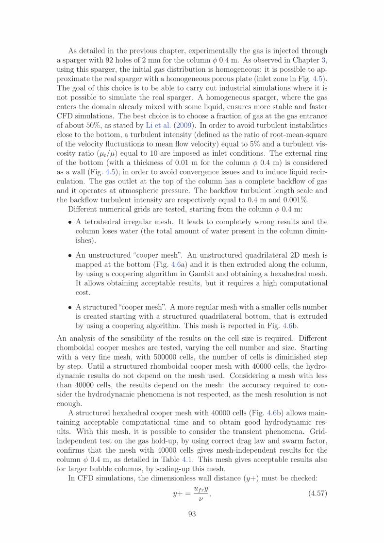
As detailed in the previous chapter, experimentally the gas is injected througha sparger with 92 holes of 2 mm for the column φ 0.4 m. As observed in Chapter 3,using this sparger, the initial gas distribution is homogeneous: it is possible to ap-proximate the real sparger with a homogeneous porous plate (inlet zone in Fig. 4.5).The goal of this choice is to be able to carry out industrial simulations where it isnot possible to simulate the real sparger. A homogeneous sparger, where the gasenters the domain already mixed with some liquid, ensures more stable and fasterCFD simulations. The best choice is to choose a fraction of gas at the gas entranceof about 50%, as stated by Li et al. (2009). In order to avoid turbulent instabilitiesclose to the bottom, a turbulent intensity (defined as the ratio of root-mean-squareof the velocity fluctuations to mean flow velocity) equal to 5% and a turbulent vis-cosity ratio (μt/μ) equal to 10 are imposed as inlet conditions. The external ringof the bottom (with a thickness of 0.01 m for the column φ 0.4 m) is consideredas a wall (Fig. 4.5), in order to avoid convergence issues and to induce liquid recir-culation. The gas outlet at the top of the column has a complete backflow of gasand it operates at atmospheric pressure. The backflow turbulent length scale andthe backflow turbulent intensity are respectively equal to 0.4 m and 0.001%.
Different numerical grids are tested, starting from the column φ 0.4 m:
• A tetrahedral irregular mesh. It leads to completely wrong results and thecolumn loses water (the total amount of water present in the column dimin-ishes).
• An unstructured “cooper mesh”. An unstructured quadrilateral 2D mesh ismapped at the bottom (Fig. 4.6a) and it is then extruded along the column,by using a coopering algorithm in Gambit and obtaining a hexahedral mesh.It allows obtaining acceptable results, but it requires a high computationalcost.
• A structured “cooper mesh”. A more regular mesh with a smaller cells numberis created starting with a structured quadrilateral bottom, that is extrudedby using a coopering algorithm. This mesh is reported in Fig. 4.6b.
An analysis of the sensibility of the results on the cell size is required. Differentrhomboidal cooper meshes are tested, varying the cell number and size. Startingwith a very fine mesh, with 500000 cells, the number of cells is diminished stepby step. Until a structured rhomboidal cooper mesh with 40000 cells, the hydro-dynamic results do not depend on the mesh used. Considering a mesh with lessthan 40000 cells, the results depend on the mesh: the accuracy required to con-sider the hydrodynamic phenomena is not respected, as the mesh resolution is notenough.
A structured hexahedral cooper mesh with 40000 cells (Fig. 4.6b) allows main-taining acceptable computational time and to obtain good hydrodynamic res-ults. With this mesh, it is possible to consider the transient phenomena. Grid-independent test on the gas hold-up, by using correct drag law and swarm factor,confirms that the mesh with 40000 cells gives mesh-independent results for thecolumn φ 0.4 m, as detailed in Table 4.1. This mesh gives acceptable results alsofor larger bubble columns, by scaling-up this mesh.
In CFD simulations, the dimensionless wall distance (y+) must be checked:
y+ =ufry
ν, (4.57)
93

(a) Irregular 1 cm.
(b) Regular 2 cm.
Figure 4.6: Cooper meshes.
94

vsg, m/s 0.03 0.06 0.09 0.16 0.25 0.35Experimental 12.8% 20.0% 20.8% 26.3% 32.2% 37.3%500000 cells 12.5% 17.4% 19.0% 24.2% 30.1% 33.8%150000 cells 12.4% 17.3% 19.0% 24.1% 29.8% 34.1%40000 cells 12.6% 17.3% 18.9% 24.1% 29.6% 34.1%10000 cells 12.1% 16.9% 22.0% 24.8% 26.8% 29.9%
Table 4.1: Grid-independent test on the gas hold-up, by using correct drag lawand swarm factor, for the column φ 0.4 m with different structured cooper meshes.
where ufr is the friction velocity at the nearest wall, y is the distance to the nearestwall and ν is the local kinematic viscosity.
It should range from 30 to 300. It affects wall shear force, pressure drop andwall lubrication force. In a large volume, y+ is not the most important parameter.By using the structured cooper mesh with 40,000 cells, the values of y+ range from30 to 500. In this work, drag force eclipses the effects of the wall forces. Walltreatments and y+ can be neglected. For this reason, standard wall functions areadopted in this work.
To scale-up this bubble column, the scale-up criteria proposed by Wilkinsonet al. (1992) ought to be respected, as stated by Besagni et al. (2018):
• “The diameter of the bubble column must be larger than 0.15 m”.This criterion is satisfied for the columns φ 0.4 m, φ 1 m and φ 3 m. Theφ 0.15 m column is the limit of the criterion and it could cause discrepancies.
• “The aspect ratio must be larger than 5”.Concerning this point, the definition of the aspect ratio is important (Sasakiet al. 2016, 2017, Besagni et al. 2017). Some authors defined the aspect ratioin terms of the column height, while other authors define the aspect ratioin function of the initial liquid level. If the total height of the column isconsidered, the studied bubble columns have an aspect ratio that is higherthan 8 and then they respect largely the criterion. If the initial liquid level isconsidered, the simulations are slightly below the criterion limit, as the initialliquid level is equal to 4 diameters. Under these operating conditions, Forret(2003) stated that the aspect ratio between operating liquid level (aeratedheight) and column diameter ought to be higher than 4. Due to the presenceof high gas volume fractions in the studied systems, the operating liquid levelis about 5 or 6 diameters. This criterion is respected if the actual operatingliquid level is considered.
• “The holes of gas sparger larger than 1-2 mm”.This criterion is satisfied for the three biggest columns (φ 0.4 m, φ 1 m andφ 3 m). These columns provide similar hydrodynamic results. The smallestcolumn (φ 0.15 m) has a sparger with holes of 1 mm. This column is at thelimits of the first and third criteria. For these reasons, some hydrodynamicdifferences could appear, compared with the other columns.
95

4.4 Results and discussion
4.4.1 Drag law and swarm factor
Calculations are validated by comparing CFD results with those obtained exper-imentally. The simulations are initially carried out on the column φ 0.4 m andfor different superficial gas velocities with demineralised water. RNG k − ε modelis initially used; later other turbulence models are tested. The global gas volumefraction is the first parameter to analyse for studying the quality of drag laws andswarm factors.
The first simulations use the drag law of Schiller & Naumann (1935) for sphericalbubbles (See Annex B for the complete study). At low superficial gas velocities(0.03 m/s, 0.09 m/s and 0.16 m/s) the computed global gas volume fraction islower than the experimental one (Fig. 4.7). At higher superficial gas velocities, the
0
20
40
60
80
0 10 20 30
Glo
bal g
as h
old-
up, %
Superficial gas velocity, cm/s
Figure 4.7: Comparison between experimental (�) and CFD gas hold-up fordifferent superficial gas velocities in the column φ 0.4 m using the drag laws ofSchiller & Naumann (1935) (�), Tomiyama (1998) (�) and Zhang et al. (2006)
(�) without swarm factor.
gas hold-up obtained with CFD simulations is higher than with experiments. Itcould mean that the drag law is too weak for low superficial gas velocities, but it istoo strong for high superficial gas velocities. A drag law for oblate bubbles is thenrequired.
The same simulations are carried out with the drag law of Tomiyama (1998),that is the most common for oblate bubbles. CFD simulations with this drag lawresult always in very high gas volume fractions, for any superficial gas velocityinvestigated, except for 0.03 m/s (Fig. 4.7). Similar results are obtained with thedrag law proposed by Zhang et al. (2006) (Fig. 4.7). The inaccuracy of these modelsis wide, with the liquid reaching the top of the domain already for a superficial gasvelocity equal to 0.16 m/s. The tendencies are however good: the global gas hold-up
96

is increasing with the gas velocity. It is useless to analyse the radial profile for thesesimulations, as the gas hold-up results are completely wrong. The drag coefficientis always too high: it is necessary to consider a swarm factor. Every simulationperformed with a drag law for oblate bubbles and without swarm factors, leads toan overestimation of the gas hold-up in the case of heterogeneous regime.
The swarm factors that increase the drag force coefficient cannot be used. Inthe case of heterogeneous regime, the swarm factor ought to be lower than unity,in order to decrease the drag force for high gas volume fractions. The swarm factorproposed by Simonnet et al. (2008) (Equation 4.19) has this characteristic. Thisswarm factor is studied in this work and coupled with the drag law proposed byTomiyama (1998). The gas hold-up predicted by implementing the swarm factoris lower than the experimental one (Fig. 4.8).
0
10
20
30
0 10 20 30
Glo
bal g
as h
old-
up, %
Superficial gas velocity, cm/s
Figure 4.8: Comparison between experimental (�) and CFD gas hold-up in thecolumn φ 0.4 m for different superficial gas velocities by using the drag law ofTomiyama (1998), considering the swarm factor of Simonnet et al. (2008) (�),
the swarm factor of McClure et al. (2014) (�), the swarm factor of McClure et al.(2017b) (�) and the new swarm factor (�).
The swarm factor of Simonnet et al. (2008) has a too strong effect for highgas volume fractions. If this swarm factor is used, some difficulties of convergencealso appear. The instantaneous behaviour of the gas volume fraction is wrong, asshown in Fig. 4.9. Some huge accumulations of gas appear in these simulations,while these huge accumulations were not found in the experiments. In these CFDsimulations, the bubbles create areas where there is only gas and areas wherethere is only water. This non-physical behaviour could be due to the asymptoticvalue of the swarm factor of Simonnet et al. (2008) in the case of very high gasvolume fraction, in which this swarm factor is close to zero. Simonnet et al. (2008)validated this empirical swarm factor only for gas volume fractions lower than 30%.It is likely unsuitable for gas fractions greater than 30%. In CFD simulations, localand instantaneous gas volume fractions exceed this value, due to fluctuations. If
97

the local gas volume fraction is greater than 30%, the drag force decreases to almostzero and causes the unphysical formation of large accumulations of bubbles.
0
20
40
60
80
100
-1 -0.5 0 0.5 1Radial position
(3)
(a) Swarm factor of Simonnet et al. (2008).
0
20
40
60
80
100
-1 -0.5 0 0.5 1Radial position
(3)
(b) New swarm factor.
Figure 4.9: Gas volume fraction for the column φ 0.4 m for a superficial gasvelocity of 0.16 m/s: (1) instantaneous behaviour, (2) sampled behaviour and
(3) instantaneous radial profile at H/D=2.5..
McClure et al. (2014) modified the swarm factor proposed by Simonnet et al.(2008). They used the Favre-averaged model proposed by Burns et al. (2004) for theturbulent diffusion, the drag law of Grace et al. (1976) coupled with the modifiedswarm factor, the k-ε model for turbulence and additional turbulence source termsdue to energy transfer from gas to liquid (Pfleger & Becker 2001). Unphysical hugeaccumulations of bubbles are absent, thanks also to the Favre-averaged turbulentdiffusion model and turbulence source terms.
McClure et al. (2017b) criticized the swarm factors of Simonnet et al. (2008)and McClure et al. (2014) for high gas volume fractions. Alternatively, McClureet al. (2017b) suggested an alternative empirical swarm factor (Equation 4.21).
98

Unphysical huge accumulations of bubbles are absent, but the global gas volumefraction is not well-predicted for each operating condition. McClure et al. (2017b)stated that this swarm factor predicts correctly the hydrodynamic properties onlyfor high gas volume fractions.
The goal of this part of the work is to obtain a global swarm factor that fitswell the experimental data for every operating condition. To achieve this goal, theswarm factor of Simonnet et al. (2008) is modified, adding a minimum constantvalue. The new swarm factor is identical to the correlation of Simonnet et al. (2008)up to 30%, but, instead of decreasing down to zero at higher gas volume fractions,it has a constant value:
h = max
⎧⎨⎩(1− αg)
[(1− αg)
25 +
(4.8
αg
1− αg
)25]− 2
25
, hmin
⎫⎬⎭ . (4.58)
Several minimum constant values (hmin) are tested. For different superficial gasvelocities, the column φ 0.4 m gives CFD results that are in good agreement withthe experiments if hmin is equal to 0.15 (Fig. 4.8). As shown in Fig. 4.9, hugeaccumulations of bubbles are absent: there are only fluctuations and preferentialbubble paths, in which the air fraction is quite bigger. The instantaneous behaviourof the CFD simulations is in good agreement with the experiments.
The other bubble columns are simulated with the swarm factor reported inEq. (4.58): φ 0.15 m, φ 1 m and φ 3 m. In order to keep the cell numberconstant, the column φ 0.4 m is scaled without modifying the mesh. By scaling-up,the differences are lower than 10% and consequently lower than the experimentalerror. The differences between experiments and CFD results are small, as shownin Fig. 4.10. A fine tuning of hmin would be possible between 0.12 and 0.18 to fitsimulations to experiments at every scale, but it is preferable to use a fixed value(hmin=0.15) for scaling-up purposes. The discrepancies are slightly higher withthe column φ 0.15 m. This column is at the limit of two Wilkinson et al. (1992)scale-up criteria, as detailed above. For these reasons, the results obtained withthis column have some discrepancies. Other methods are required for scaling-downthese systems.
As observed in Fig. 4.11, the radial profile of gas volume fraction is almost flatunder the homogeneous regime (0.03 m/s) and it is parabolic under the heterogen-eous regime (0.16 m/s). It allows recognizing the flow regime.
The axial liquid velocity strongly influences the mixing processes and it is animportant parameter for bioreactors, in which shear stress and high velocities candamage the biomass, lowering the efficiency. The axial liquid velocity in the columncentre obtained with CFD simulations is compared with that of experiments ofForret (2003), as shown in Fig. 4.12. These results are compared also with thecorrelation of Miyauchi & Shyu (1970) (Fig. 4.12). The radial profiles of axialliquid velocity are well-predicted with the new swarm factor (Fig. 4.13). By usingthe new swarm factor, CFD and experimental liquid velocity profiles are almostidentical for every operating condition investigated in this study. The liquid velocitystrongly depends on the drag law and swarm factor. As the liquid velocity profileis well-predicted, this new swarm factor, coupled with the drag law proposed byTomiyama (1998), can be considered as correct. Consequently, this swarm factoris used in the following parts of this work.
99

0
10
20
30
0 10 20 30
Com
puta
tiona
l glo
bal g
as h
old-
up, %
Experimental global gas hold-up, %
Figure 4.10: Scale-up effect on the gas hold-up using the Tomiyama (1998) draglaw and the new swarm factor (hmin=0.15). Parity graph for the gas hold-upbetween experimental (Raimundo 2015) and CFD data for different columns:
φ 0.15 m (�), φ 0.4 m (�), φ 1 m (�) and φ 3 m (�).
The physical meaning of the proposed swarm factor is not fully understood.Very complex interactions between bubbles and large turbulent eddies occur. Con-sequently, the resulting drag law, coupled with the swarm factor, can be consideredas an integrated interfacial exchange term. It is considered as a drag force as it isthe main force involved, but it includes probably other interfacial forces.
Standard k-ε, realizable k-ε, RNG k-ε and k-ω models are compared. The firsttwo models give numerical errors in the case of high superficial gas velocities. Thefirst model slightly overestimates the gas fraction in the column centre and under-estimates the axial liquid velocity in the column centre in the case of heterogeneousregime, as reported in Fig. 4.14. Realizable k-ε model gives a well-predicted gasvolume fraction profile and the axial liquid velocity in the column centre is under-estimated, as detailed in Fig. 4.14. RNG k-ε model provides better and more stableresults. With this model, gas volume fraction profile and axial liquid velocity inthe column centre are well-predicted. The k-ω provides radial profiles of local gasvolume fraction and axial liquid velocity very similar to those obtained with RNGk-ε model, as reported in Fig. 4.14. RNG k-ε and k-ω models seem to be the bestones due to their stability and thus they are used in the following parts of thiswork.
100

0
10
20
30
0 0.2 0.4 0.6 0.8 1
Loca
l gas
vol
ume
fract
ion,
%
Radial position
(a) φ 0.4 m
0
10
20
30
0 0.2 0.4 0.6 0.8 1
Loca
l gas
vol
ume
fract
ion,
%
Radial position
(b) φ 1 m
Figure 4.11: Experimental versus CFD sampled radial profiles of the gas volumefraction at H/D=2.5 using the new swarm factor for a superficial gas velocity
equal to 0.03 m/s (experimental (�) vs CFD (dashed line)) and 0.16 m/s(experimental (�) vs CFD (solid line)).
101

0
0.5
1
1.5
0 0.1 0.2 0.3
Axi
al li
quid
vel
ocity
, m/s
Superficial gas velocity, m/s
(a) φ 0.4 m
0
0.5
1
1.5
0 0.1 0.2 0.3
Axi
al li
quid
vel
ocity
, m/s
Superficial gas velocity, m/s(b) φ 1 m
Figure 4.12: Axial liquid velocity in the centre at H/D=3.75: experimental data ofForret (2003) (�) versus CFD data obtained using the new swarm factor (� and
solid line) versus correlation of Miyauchi & Shyu (1970) (dotted line).
102

-1
-0.5
0
0.5
1
0 0.2 0.4 0.6 0.8 1
Axi
al li
quid
vel
ocity
, m/s
Radial position
(a) φ 0.4 m
-1
-0.5
0
0.5
1
0 0.2 0.4 0.6 0.8 1Radial position
(b) φ 1 m
Figure 4.13: Experimental versus CFD sampled radial profiles of the liquidvelocity using the new swarm factor at H/D=3.75 for a superficial gas velocity
equal to 0.03 m/s (experimental (�) vs CFD (dashed line)) and 0.16 m/s(experimental (�) vs CFD (solid line)).
103

0
10
20
30
40
0 0.2 0.4 0.6 0.8 1
Loca
l gas
frac
tion,
%
Radial position
(a) Gas volume fraction at H/D=2.5.
-1
-0.5
0
0.5
1
0 0.2 0.4 0.6 0.8 1
Axi
al li
quid
vel
ocity
, m/s
Radial position
(b) Axial liquid velocity at H/D=3.75.
Figure 4.14: Turbulence models comparison of the hydrodynamic properties forthe column φ 0.4 m and a superficial gas velocity of 0.16 m/s: standard k-ε (dashdot line), realizable k-ε (dotted line), RNG k-ε (solid line) and k-ω (dashed line).
104

4.4.2 Mixing time
An additional transport equation is used to simulate the mixing of a scalar quant-ity. The normalised concentration is used as additional transport equation. Mixingtime is defined as the time necessary to reach a predefined level of homogeneity, i.e.a deviation of 5% from the final concentration. The mixing time results obtainedusing the RNG k-ε and the k-ω models are compared in Fig. 4.15 with the exper-imental data of (Forret 2003). The tracer response data are available only for thecolumn φ 1 m. The diffusion coefficient is defined in three different ways for eachsimulation: considering only the molecular diffusivity, adding only SIT or consider-ing SIT with bubble contribution. CFD curves are obtained by averaging the scalarconcentration over the column section at the same height of the experiments. Thecases simulated with only the molecular diffusivity term in the transport equationare wrong, while the other CFD cases are in good agreement with the values of theexperiments. Bubble contribution does not have a great impact on the mixing timewith both the turbulence models. The RNG k-ε predicts well the concentrationevolution over time (Fig. 4.15). Mixing times obtained with RNG k-ε simulationsunder the heterogeneous regime are listed in Table 4.2.
superficial gas velocity 0.09 m/s 0.16 m/s 0.25 m/sBubble contribution yes no yes no yes no
φ 0.4 m 6.70 7.70 4.70 5.50 3.40 3.60φ 1 m 12.30 12.40 10.20 11.10 5.38 5.35φ 3 m 36.70 37.75 31.08 31.22 23.20 23.33
Table 4.2: Mixing time (in seconds) using RNG k-ε and diffusivity model ofAlméras et al. (2016) for different bubble columns.
These results confirm that bubble contribution on trasport of scalars has notgreat effects, except for the column φ 0.4 m, as shown in Fig. 4.16: a differenceof about 10% appears if the superficial gas velocity is lower than 0.16 m/s. Thebubble contribution should be taken into account for small-scale systems, as statedby Alméras et al. (2015). The time evolution of the scalar concentration field isrepresented in Fig. 4.17.
By using the model of Pfleger & Becker (2001) for considering turbulence dueto energy transfer from gas to liquid, McClure et al. (2014) obtained good resultsfor a column of 0.19 m with a square perforated sparger. McClure et al. (2014)obtained a gas volume fraction profile similar to the experimental data. In thiswork, the hydrodynamics is well-predicted without additional source terms in thek and ε transport equations. McClure et al. (2014) used ANSYS CFX, while theCFD simulations are realized with ANSYS Fluent in the present work. Fletcheret al. (2017) proved that, if identical closure models are used, the choice of thesoftware does not affect the results. Different operating conditions and differentgeometries have been tested: it could be a partial explanation.
The proposed swarm factor allows obtaining computational results in goodagreement with the experiments. Huge accumulations of bubbles are absent andthe instantaneous preferential paths for bubbles (Fig. 4.9) simulate the creation ofexperimental instantaneous bubble macro-structure. The drag force contribution
105

0
0.5
1
1.5
0 5 10 15 20
Nor
mal
ized
con
cent
ratio
n
Time, s(a) RNG k-ε.
0
0.5
1
1.5
0 5 10 15 20
Nor
mal
ized
con
cent
ratio
n
Time, s(b) k-ω.
Figure 4.15: Normalized concentration for the column φ 1 m and a superficial gasvelocity of 0.15 m/s. Comparison of the experimental data of Forret (2003) (�)with the CFD simulations using molecular diffusivity only (dotted line), SIT
(dash dot line) and SIT + bubble contribution (solid line).
106

0
5
10
15
0 0.1 0.2 0.3
Mix
ing
time,
s
Superficial gas velocity, cm/s(a) φ 0.4 m
0
5
10
15
0 0.1 0.2 0.3
Mix
ing
time,
s
Superficial gas velocity, cm/s(b) φ 1 m
Figure 4.16: Mixing time as a function of the superficial gas velocity, calculatedby using the RNG k-ε model coupled with SIT (dash dot line) and SIT + bubble
contribution (solid line). Comparison with the experimental data collected byForret (2003) (�).
107

Figure 4.17: Snapshots of the scalar concentration field with RNG k-ε andAlméras et al. (2015) models for the column φ 0.4 m and a superficial gas velocityequal to 0.15 m/s at different times: t=0, 2, 4, 6, 8, 10, 12, 14 s from left to right.
influences the hydrodynamic behaviour and thus the mixing time. More effortswill be required to fully understand the additional turbulence due to the energytransfer from gas phase to liquid phase.
Column diameter and superficial gas velocity strongly influence the mixing time.In Fig. 4.18 and in Fig. 4.19, mixing time is presented as a function of column dia-meter and superficial gas velocity for both k-ω and RNG k-ε models; furthermore,the Alméras et al. (2015) turbulent diffusivity model is considered. Mixing time islow for high superficial gas velocities. Bigger columns require higher mixing time.The turbulence model choice has stronger effects when column diameter increases.
The turbulent viscosity appears directly in the diffusion coefficient and thenit is an important parameter to model the scalar transport. In Fig. 4.20, thesimulated viscosity is compared with several correlations. The best agreement isobtained with the correlation proposed by Kawase & Moo-Young (1989), whilehigher discrepancies appear with the correlations of Miyauchi & Shyu (1970) andBurns & Rice (1997). Guédon et al. (2017) arrived at the same conclusions.
Furthermore, turbulent kinematic viscosities obtained by using RNG k-ε and k-ω models, are compared in Fig. 4.20. Turbulent kinematic viscosity obtained withthe k-ω is almost twice that obtained with the RNG k-ε. Mixing time computedwith the RNG k-ε is lower. These aspects could appear in contradiction, but thisbehaviour can be explained by considering that there is the convective transport inaddition to the diffusive phenomena. If only the molecular diffusion of the scalaris considered, the mixing time is longer. For the k-ω, the mixing time increase ishigher, so it can be concluded that the macro recirculation is stronger for the RNGk-ε model, and it causes a quicker tracer mixing into the bubble column, even ifthe turbulent dispersion is lower with this turbulence model.
108

0
10
20
30
40
50
0 0.5 1 1.5 2 2.5 3
Mix
ing
time,
s
Column diameter, m
Figure 4.18: Mixing time as a function of the column diameter. Comparisonbetween two different turbulence models: RNG k-ε (� 0.09 m/s, � 0.16 m/s and
� 0.25 m/s) and k-ω (� 0.09 m/s, � 0.16 m/s m and � 0.25 m/s).
0
10
20
30
40
50
0 0.1 0.2 0.3
Mix
ing
time,
s
Superficial gas velocity, m/s
Figure 4.19: Mixing time as a function of the superficial gas velocity. Comparisonbetween two different turbulence models: RNG k-ε (� φ 0.4 m, � φ 1 m and
� φ 3 m) and k-ω (� φ 0.4 m, � φ 1 m and � φ 3 m).
109
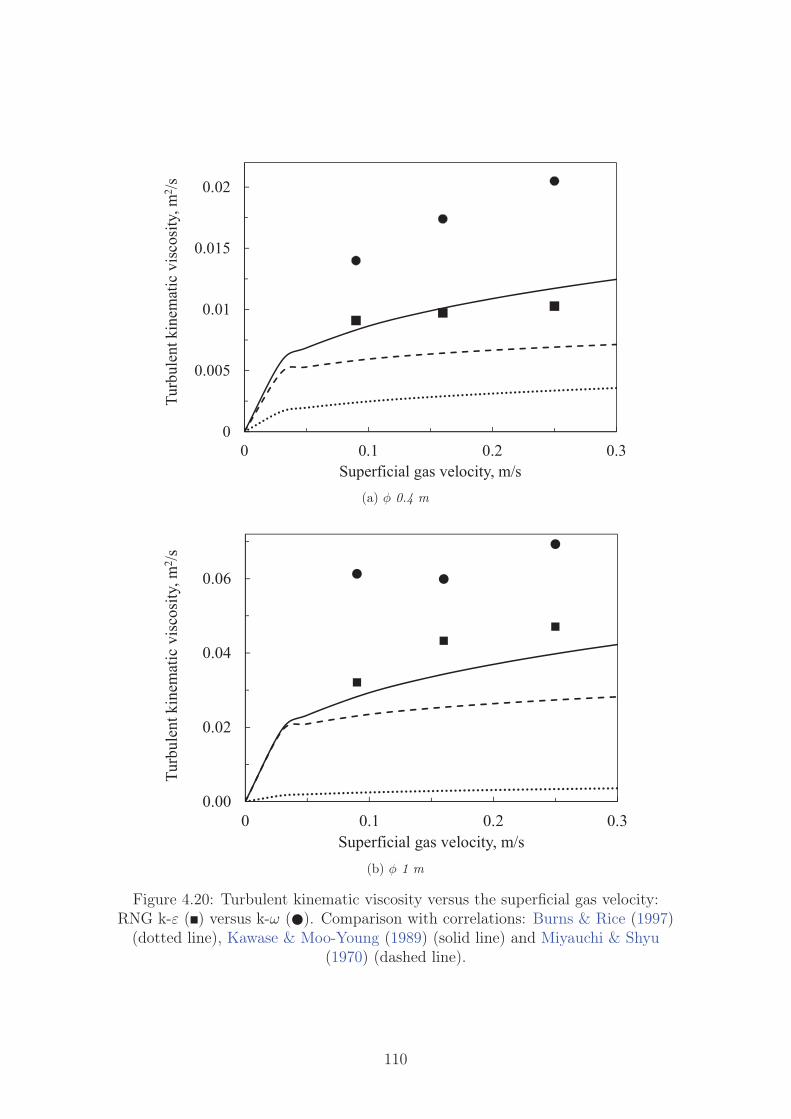
0
0.005
0.01
0.015
0.02
0 0.1 0.2 0.3
Turb
ulen
t kin
emat
ic v
isco
sity
, m2 /s
Superficial gas velocity, m/s(a) φ 0.4 m
0.00
0.02
0.04
0.06
0 0.1 0.2 0.3
Turb
ulen
t kin
emat
ic v
isco
sity
, m2 /s
Superficial gas velocity, m/s(b) φ 1 m
Figure 4.20: Turbulent kinematic viscosity versus the superficial gas velocity:RNG k-ε (�) versus k-ω (�). Comparison with correlations: Burns & Rice (1997)
(dotted line), Kawase & Moo-Young (1989) (solid line) and Miyauchi & Shyu(1970) (dashed line).
110

4.5 Conclusions and perspectivesTransient 3D simulations are required to simulate bubble columns under the het-erogeneous flow regime. Gas-liquid interactions are dominated by interfacial forces.The drag force is the most important interfacial force for these systems. A drag lawsuitable for oblate bubbles needs to be used. The drag law proposed by Tomiyama(1998) has a wide range of validity and it has the advantage that it can considercontamination effects. For high gas volume fractions, the original drag law oughtto be modified considering a swarm factor in order to decrease the drag force effect.The experimental swarm factor of Simonnet et al. (2008) has this characteristic,but its effect is too strong and the instantaneous behaviour is not well-predicted:unphysical huge accumulations of bubbles appear in the column. This swarm factorcan be used for a gas volume fraction up to 30%. This value is instantaneouslyovercome and then the swarm factor of Simonnet et al. (2008) needs to be modified.
By adding a minimum value at the swarm factor of Simonnet et al. (2008)(Equation 4.58), the CFD results are in good agreement with the experimental data.The instantaneous behaviour is correct: unphysical huge accumulations of bubblesare absent. The CFD simulations are stable. The radial profiles of gas volumefraction and liquid velocity are well-predicted. A constant value of hmin=0.15 issuggested. The discrepancy between experimental data and CFD results is verysmall in the case of big bubble columns and then this swarm factor can be used forscaling-up purposes.
An extra diffusion coefficient due to the presence of bubbles (Alméras et al.2015) is considered in the scalar transport equation to study the mixing time.Shear-induced turbulence is the dominant contribution in mixing processes. TheRNG k-ε turbulence model predicts a mixing time that is similar to the exper-imental one. Mixing time is higher if only the molecular diffusion is consideredto model diffusivity. Bubble contribution is often negligible for big columns. Thediffusion due to the presence of bubbles has a significant effect on scalar mixing forsmall columns and, in these cases, the diffusive model of Alméras et al. (2015) im-proves the numerical results. Bubble contribution should be considered for bubblecolumns with a diameter up to 0.4 m.
Secondary interfacial forces, neglected in this work, near wall treatments andother boundary conditions could be considered.
111

Bibliography
Alméras, E., Plais, C., Euzenat, F., Risso, F., Roig, V. & Augier, F. (2016), ‘Scalarmixing in bubbly flows: Experimental investigation and diffusivity modelling’,Chemical Engineering Science 140, 114–122.
Alméras, E., Risso, F., Roig, V., Cazin, S., Plais, C. & Augier, F. (2015), ‘Mixingby bubble-induced turbulence’, Journal of Fluid Mechanics 776, 458–474.
Andersson, B., Andersson, R., Håkansson, L., Mortensen, M., Sudiyo, R., Van Wa-chem, B. & Hellström, L. (2012), Computational Fluid Dynamics for Engineers,first edn, University Press, Cambridge, UK.
Besagni, G., Di Pasquali, A., Gallazzini, L., Gottardi, E., Colombo, L. P. M.& Inzoli, F. (2017), ‘The effect of aspect ratio in counter-current gas-liquidbubble columns: Experimental results and gas holdup correlations’, Interna-tional Journal of Multiphase Flow 94, 53–78.
Besagni, G., Gallazzini, L. & Inzoli, F. (2018), ‘On the scale-up criteria for bubblecolumns’, Petroleum .
Bird, R. B., Stewart, W. E. & Lightfoot, E. N. (2007), Transport Phenomena,revised second edn, John Wiley & Sons, Inc., New York, NJ.
Boussinesq, J. (1897), Théorie de l’écoulement tourbillonnant et tumultueux desliquides dans les lits rectilignes à grande section, Gauthier-Villars et fils.
Bridge, A. G., Lapidus, L. & Elgin, J. C. (1964), ‘The mechanics of vertical gas-liquid fluidized system i: Countercurrent flow’, American Institute of ChemicalEngineering Journal 10(6), 819–826.
Buffo, A. & Marchisio, D. L. (2014), ‘Modeling and simulation of turbulent poly-disperse gas-liquid systems via the generalized population balance equation.’,Reviews in Chemical Engineering 30, 73–126.
Burns, A. D., Frank, T., Hamill, I. & Shi, J. M. (2004), The favre averaged dragmodel for turbulent dispersion in eulerian multi-phase flows, in ‘5th InternationalConference on Multiphase Flow.’, Yokohama, Japan.
Burns, L. F. & Rice, R. G. (1997), ‘Circulation in bubble columns’, AmericanInstitute of Chemical Engineering Journal 43(6), 1390–1402.
Cappello, V. (2016), Simulation of heterogeneous flow in large bubble column withmixing of species, Master thesis, Politecnico di Torino, Torino.
Clift, R., Grace, J. R. & Weber, M. E. (1978), Bubbles, Drops, and Particles,Academic Press.
Combest, D. P., Ramachandran, P. A. & Dudukovic, M. P. (2011), ‘On the gradientdiffusion hypothesis and passive scalar transport in turbulent flows’, Industrial& Engineering Chemistry Research 50(15), 8817–8823.
112
Ekambara, K., Dhotre, M. T. & Joshi, J. B. (2005), ‘CFD simulations of bubblecolumn reactors: 1D, 2D and 3D approach’, Chemical Engineering Science60(23), 6733–6746.
Elghobashi, S. E. & Abou-Arab, T. W. (1983), ‘A two-equation turbulence modelfor two-phase flows’, Physics of Fluids 26, 931–938.
Fletcher, D. F., McClure, D. D., Kavanagh, J. M. & Barton, G. W. (2017), ‘CFDsimulation of industrial bubble columns: Numerical challenges and model valid-ation successes’, Applied Mathematical Modelling 44, 25–42.
Forret, A. (2003), Hydrodynamics scale-up of slurry bubble columns, PhD thesis,Université Claude Bernard Lyon 1-IFPEN, Lyon.
Gemello, L., Plais, C., Augier, F., Cloupet, A. & Marchisio, D. L. (2018), ‘Hy-drodynamics and bubble size in bubble columns: Effects of contaminants andspargers’, Chemical Engineering Science 184, 93–102.
Grace, J., Wairegi, T. & Nguyen, T. H. (1976), ‘Shapes and velocities of singledrops and bubbles moving freely through immiscible liquids’, Transactions ofthe Institution of Chemical Engineers 54, 167–173.
Guédon, G. R., Besagni, G. & Inzoli, F. (2017), ‘Prediction of gas-liquid flow inan annular gap bubble column using a bi-dispersed eulerian model’, ChemicalEngineering Science 161, 138–150.
Hillmer, G., Weismantel, L. & Hofmann, H. (1994), ‘Investigations and modellingof slurry bubble columns’, Chemical Engineering Science 49(6), 837–843.
Hlawitschka, M., Kováts, P., Zähringer, K. & Bart, H.-J. (2017), ‘Simulation andexperimental validation of reactive bubble column reactors’, Chemical Engineer-ing Science 170, 306–319.
Ishii, M. & Zuber, N. (1979), ‘Drag coefficient and relative velocity in bubbly,droplet or particulate flows’, American Institute of Chemical Engineering Journal25(5), 843–855.
Jakobsen, H. A., Lindborg, H. & Dorao, C. A. (2005), ‘Modeling of bubble columnreactors: Progress and limitations’, Industrial & Engineering Chemistry Research44(14), 5107–5151.
Joshi, J. B. (2001), ‘Computational flow modelling and design of bubble columnreactors’, Chemical Engineering Science 56(21), 5893–5933.
Kataoka, I., Besnard, D. C. & Serizawa, A. (1992), ‘Basic equation of turbulenceand modelling of interfacial transfer terms in gas-liquid two-phase flow’, ChemicalEngineering Communications 118, 221–236.
Kawase, Y. & Moo-Young, M. (1989), ‘Turbulence intensity in bubble columns’,The Chemical Engineering Journal 40(1), 55–58.
Launder, B. E. & Spalding, D. B. (1972), Lectures in Mathematical Models ofTurbulence., Academic Press, London, U.K.
113

Li, G., Yang, X. & Dai, G. (2009), ‘CFD simulation of effects of the configurationof gas distributors on gas-liquid flow and mixing in a bubble column’, ChemicalEngineering Science 64(24), 5104–5116.
McClure, D. D., Dolton, T. P., Barton, G. W., Fletcher, D. F. & Kavanagh, J. M.(2017a), ‘Hydrodynamics and mixing in airlift contactors: Experimental workand CFD modelling’, Chemical Engineering Research and Design 127, 154–169.
McClure, D. D., Kavanagh, J. M., Fletcher, D. F. & Barton, G. W. (2013), ‘De-velopment of a CFD model of bubble column bioreactors: Part one - A detailedexperimental study’, Chemical Engineering & Technology 36(12), 2065–2070.
McClure, D. D., Kavanagh, J. M., Fletcher, D. F. & Barton, G. W. (2017b),‘Experimental investigation into the drag volume fraction correction term forgas-liquid bubbly flows’, Chemical Engineering Science 170, 91–97.
McClure, D. D., Norris, H., Kavanagh, J. M., Fletcher, D. F. & Barton, G. W.(2014), ‘Validation of a computationally efficient computational fluid dynamics(CFD) model for industrial bubble column bioreactors’, Industrial & EngineeringChemistry Research 53(37), 14526–14543.
Miyauchi, T. & Shyu, C.-N. (1970), ‘Flow of fluid in gas bubble columns’, KagakuKogaku 34(9), 958–964.
Pfleger, D. & Becker, S. (2001), ‘Modeling and simulation of the dynamic flowbehavior in a bubble column’, Chemical Engineering Science 56, 1737–1747.
Radl, S. & Khinast, J. G. (2010), ‘Multiphase flow and mixing in dilute bubbleswarms’, American Institute of Chemical Engineering Journal 56, 2421–2445.
Raimundo, P. M. (2015), Analysis and modelization of local hydrodynamics inbubble columns, PhD thesis, Université Grenoble Alpes.
Ranade, V. (1997), ‘Modelling of turbulent flow in a bubble column reactor’, Chem-ical Engineering Research and Design 75(1), 1– 23. Process and Product Devel-opment.
Roghair, I., Lau, Y. M., Deen, N. G., Slagter, H. M., Baltussen, M. W., VanSint Annaland, M. & Kuipers, J. A. M. (2011), ‘On the drag force of bubbles inbubble swarms at intermediate and high reynolds numbers’, Chemical Engineer-ing Science 66, 3204–3211.
Rusche, H. & Issa, R. (2000), The effect of voidage on the drag force on particles,droplets and bubbles in dispersed two-phase flow, in ‘2nd Japanese EuropeanTwo-Phase Flow Meeting.’, Tsukuba, Japan.
Rzehak, R. & Krepper, E. (2013), ‘CFD modeling of bubble-induced turbulence’,International Journal of Multiphase Flow 55, 138–155.
Sasaki, S., Hayashi, K. & Tomiyama, A. (2016), ‘Effects of liquid height on gasholdup in air-water bubble column’, Experimental Thermal and Fluid Science72, 67–74.
114

Sasaki, S., Uchida, K., Hayashi, K. & Tomiyama, A. (2017), ‘Effects of columndiameter and liquid height on gas holdup in air-water bubble columns’, Experi-mental Thermal and Fluid Science 82, 359–366.
Sato, Y. & Sekoguchi, K. (1975), ‘Liquid velocity distribution in two-phase bubbleflow’, International Journal of Multiphase Flow 2(1), 79–95.
Schiller, L. & Naumann, N. (1935), ‘A drag coefficient correlation.’, Vdi Zeitung77, 318.
Shah, Y. T., Kelkar, B. G., Godbole, S. P. & Deckwer, W. D. (1982), ‘Design para-meters estimations for bubble column reactors’, American Institute of ChemicalEngineering Journal 28(3), 353–379.
Shih, T. H., Liou, W. W., Shabbir, A. & Zhu, J. (1995), ‘A new k − ε eddy-viscosity model for high reynolds number turbulent flows - model developmentand validation.’, Computers Fluids 24(3), 227–238.
Simonin, O. & Viollet, P. L. (1990), ‘Modeling of turbulent two-phase jets loadedwith discrete particles’, Phenomena in Multiphase Flows pp. 259–269.
Simonnet, M., Gentric, C., Olmos, E. & Midoux, N. (2008), ‘CFD simulation of theflow field in a bubble column reactor: Importance of the drag force formulationto describe regime transitions’, Chemical Engineering and Processing: ProcessIntensification 47(9), 1726–1737.
Sugrue, R. M. (2017), A robust momentum closure approach for multiphase com-putational fluid dynamics applications, PhD thesis, Massachusetts Institute ofTechnology.
Suzzi, D., Radl, S. & Khinast, J. (2013), ‘Validation of euler-euler and euler-lagrange approaches in the simulation of bubble columns.’, Chemical EngineeringTransactions 17, 585–590.
Tabib, M. V., Roy, S. A. & Joshi, J. B. (2008), ‘CFD simulation of bubble column- An analysis of interphase forces and turbulence models’, Chemical EngineeringJournal 139(3), 589–614.
Tomiyama, A. (1998), ‘Struggle with computational bubble dynamics’, MultiphaseScience and Technology 10(4), 369.
Troshko, A. A. & Hassan, Y. A. (2001), ‘A two-equation turbulence model ofturbulent bubbly flows’, International Journal of Multiphase Flow 27(11), 1965–2000.
Vaidheeswaran, A. & Lopez de Bertodano, M. (2017), ‘Stability and convergenceof computational eulerian two-fluid model for a bubble plume’, Chemical Engin-eering Science 160, 210–226.
Versteeg, H. & Malalasekera, W. (2007), An introduction to computational fluid dy-namics: the finite volume method., 2nd edn, Pearson Education Limited, Harlow,England.
115

Wallis, G. B. (1969), One-dimensional two-phase flow, 1st edn, McGraw-Hill, NewYork.
Wilcox, D. C. (1998), Turbulence modeling for CFD., DCW Industries, Inc., LaCanada, California.
Wilkinson, P. M., Spek, A. P. & Van Dierendonck, L. L. (1992), ‘Design parametersestimation for scale-up of high pressure bubble column’, American Institute ofChemical Engineering Journal 38, 544–554.
Yakhot, V. & Orszag, S. A. (1986), ‘Renormalization group analysis of turbulencei basic theory.’, Journal of scientific computing 1(1), 1–51.
Yao, W. & Morel, C. (2004), ‘Volumetric interfacial area prediction in upward bub-bly two-phase flow’, International Journal of Heat and Mass Transfer 47, 307–328.
Zhang, D. (2007), Eulerian modeling of reactive gas-liquid flow in a bubble column,PhD thesis, Enschede, The Netherlands.
Zhang, D., Deen, N. G. & Kuipers, J. A. M. (2006), ‘Numerical simulation ofdynamic flow behavior in a bubble column: A study of closures for turbulenceand interface forces’, Chemical Engineering Science 61, 7593–7608.
116

Chapter 5
Population Balance Modelling ofheterogeneous bubble columnreactors
5.1 Introduction
Eulerian-Eulerian RANS methods allow simulating heterogeneous flows with a rel-atively low computational cost, as detailed in Chapter 4. These methods are oftenused for industrial applications. One important limitation of Eulerian-Eulerianclassical CFD models is due to the assumption that every bubble has the same sizeand that this is an input parameter for the simulation. The use of a single bubblesize hinders the prediction of local hydrodynamic properties. The polydispersity ofgas bubbles is an aspect that turns out to be very important in gas-liquid multiphaseflows: significant variations of bubble size are observed in bubble column reactors.Bubble polydispersity causes considerable variations in the interfacial area, affect-ing, in turn, the rate of exchange of mass, momentum and energy between the twophases (i.e. continuous and disperse) and between the multiphase flow and the ex-ternal boundaries. A population balance model (PBM) can be coupled with CFDsimulations to overcome these limits and make the CFD simulations more predict-ive. Classical mass, momentum and energy equations solved in multiphase flowsare coupled with population balance equations (PBEs). CFD-PBM coupling allowsconsidering the effects of bubble coalescence and breakage on the development ofthe interfacial area between the continuous and disperse phases.
The methods for solving the PBE could be distinguished into three groups:Classes (or sectional) Methods, Monte Carlo Methods and Moment-based Methodsand only some of them are suitable for CFD implementation.
In the Classes Methods (CM) the internal coordinates, for example bubble size,is discretized. These methods, firstly developed for univariate cases (see for examplethe comparison performed by Vanni (2000)), are extended to multivariate cases(Kumar et al. 2008). The discretization is performed by using different techniques,as such the finite volume method proposed by Gunawan et al. (2004), the finiteelement method proposed by Godin et al. (1999) or the finite difference method.The MUSIG method is often used for gas-liquid flows (Frank et al. 2008). Thesemethods could present however the following problem: they could require largecomputational resources, resulting in time-consuming simulations. The transport
117

of separated classes of bubbles, although displaying some advantages, is often time-consuming.
The second group, called Monte Carlo Method (MCM), solves stochastic dif-ferential equations that are capable of reproducing a finite number of artificialrealizations of the system (Zhao et al. 2007); these methods require huge compu-tational costs when coupled with CFD and they can be used only for simplifiedsimulations.
The Methods of Moments solve the transport equations for some lower-ordermoments (Marchisio et al. 2003a). In other words, instead of solving the PBE,a limited number of transport equations, derived from the PBE by applying themoment transform, are solved. These methods present a closure problem thatcan be solved through different methods. An important class of these methods isthe Quadrature-Based Moments Methods (QBMM), used in this work, where theclosure problem is overcome by using an ad-hoc quadrature approximation.
In Quadrature-Based Moments Methods (QBMM), the bubble size distribution(BSD) or Number Density Function (NDF) is assumed to be the summation of somebasis functions centred on the zeros of polynomials orthogonal to the BSD or NDF,or in other words, centred on the nodes of a Gaussian quadrature approximation.The quadrature approximation, calculated from the moments of the BSD or NDF,is more accurate than other methods in overcoming the closure problem even whenthe order of the quadrature approximation is very small (i.e. two or three). Thefinal method, that combines the use of the moments of the BSD and the use of thequadrature approximation, can be employed for coupling with CFD simulations,as a small number of additional equations is required. For a typical problem, theevolution of the BSD can be predicted only by tracking the evolution of six momentsof the BSD, corresponding to a quadrature approximation of order three. By usingthe CM to predict the evolution of the BSD with similar accuracy, 30 or 40 classes(and corresponding transport equations) might have to be solved, resulting in muchhigher computational costs (Marchisio et al. 2003b).
These methods are employed both for univariate and multivariate PBE, wherein other words, one internal coordinate (e.g. bubble size) or multiple internalcoordinates (e.g. bubble size and composition) are employed. For univariate cases,the original Quadrature Method of Moments (QMOM) (McGraw 1997) can be used.The quadrature approximation is obtained with a specific inversion algorithm.
Bubble size depends on coalescence and breakage phenomena, closely linkedto operating conditions and turbulence. These phenomena are however mainlystudied for low gas velocities (Falzone et al. 2018) and model small gas volumefraction. In this work, the objective is to go beyond current practice and developa model that simulates what happens at higher superficial gas velocities. To thisend, experimental data obtained by Gemello et al. (2018a) and detailed in Chapter3 are used. Thanks to these experimental results it is possible to investigate alsothe effects of different initial bubble sizes and the presence of additives. The maingoal of this work is to identify breakage and coalescence kernels that are capableof simulating the bubble size for both homogeneous and heterogeneous regimes.Different mechanisms are involved in bubble breakage as shown by Liao & Lucas(2009) and the main mechanism is linked to turbulent fluctuations. On the otherhand, the coalescence kernel is divided between collision frequency and coalescenceefficiency, as stated by Liao & Lucas (2010). Collisions are caused by several
118

phenomena, the turbulent fluctuations being the most important. The coalescenceefficiency can be studied with three methods: film drainage model, energy modeland critical approach velocity model; the first model is the most common for thehomogeneous regime. Existing breakage and coalescence models were developedand validated for the homogeneous regime, where there is a lack of kernels suitablefor the heterogeneous regime.
In this work, breakage and coalescence models are validated under the hetero-geneous flow regime, providing a suitable and innovative set of models that canpredict correctly the bubble size for a wide range of operating conditions.
Starting from the experimental results detailed in Chapter 3, the existing break-age and coalescence kernels, suitable for the homogeneous regime, are tested andextended for the heterogeneous regime. 3D transient Eulerian-Eulerian CFD sim-ulations with ANSYS Fluent are carried out and coupled with QMOM. 0D simu-lations with Matlab were also performed to provide a preliminary screening of thetested coalescence and breakage models.
5.2 Population Balance Modelling
The disperse phase is constituted by discrete elements (i.e. bubbles in the caseof gas-liquid systems): each element of this phase is identified by a number ofcoordinates, that are classified as internal and external. Two elements are identicalif they have identical coordinates. External coordinates are spatial coordinates andtime, while internal coordinates refer to other intrinsic properties of the elementssuch as volume, surface area, size, age, velocity and temperature (Marchisio & Fox2013).
The Number-density functions (NDF) contains information about the popu-lation of bubbles, explaining how it is distributed over the properties of interestinside an infinitesimal control volume. Let us consider an infinitesimal controlvolume located at physical point x = (x1, x2, x3) of measure dx = (dx1, dx2, dx3)and at phase-space point, ξ = (ξ1, ξ2, ξ3). The NDF nξ(t, x, ξ) identifies the pop-ulation of bubbles in the computational domain at each instant. Integrating theNDF over all possible values of the internal-coordinate vector, the total numberconcentration N(t,x) is obtained, which is the total number of entities per unitvolume located at time t at point x, and it corresponds to the moment of orderzero of the NDF:
N = mξ,0 =
∫nξ(ξ)dξ. (5.1)
Higher-order moments of the NDF can be defined:
mξ,k =
∫ξ1
k1 ...ξMkMnξ(ξ)dξ, (5.2)
where k = (k1, k2, ..., kN) . The PBE is a continuity statement expressed in termsof the NDF. The velocity of the PBE is assumed to be equal to the local velocity inthe continuous phase or derivable from this. The PBE basically counts the numberof elements (bubbles) belonging to a specific finite volume defined both in physical-space and phase-space. The number of elements inside this volume changes due tothe movement of the bubbles in physical space, their velocities, the movement of
119

the bubbles in physical space, continuous processes, and because of discontinuousor discrete events, resulting in the following equation (Marchisio & Fox 2013):
∂
∂t
(∫Ωx
dx∫Ωξ
dξ nξ
)+
∫Ωξ
dξ
∫∂Ωx
(nξu) · dAx+
+
∫Ωx
dx∫∂Ωξ
(nξξ
)· dAξ =
∫Ωx
dx∫Ωξ
dξ Sξ, (5.3)
where u is the velocity vector of the bubbles, ξ is the rate of change of the genericinternal coordinate for the bubbles, Ωx is the finite control volume in physical space,Ωξ is the finite control volume in phase space, ∂Ωx and ∂Ωξ are their boundariesand Sξ considers the discrete events, such as collisions between bubbles, leading tocoalescence or breakage and nucleation.
If the Reynolds-Gauss theorem is applied and the equality is forced to be re-spected for any possible control volumes, the following equation is obtained:
∂nξ
∂t+
∂
∂x· (unξ) +
∂
∂ξ·(ξ nξ
)= Sξ. (5.4)
A generic turbulent gas-liquid flow can be considered as a dispersion of bubbles,that are characterized by their size L, composition φb, velocity ub and possiblytemperature T . The PBE is considered univariate if the population of bubbles isdescribed by just one internal coordinate, for example bubble size or length. ThePBE is called bivariate if two internal coordinates are considered, e.g. bubble sizeand chemical composition. Higher-dimensional PBEs are referred to as multivari-ate. If the bubbles are characterized by their own velocity distribution, the PBEbecomes the generalized population-balance equation (GPBE) were bubble velocityis included in the PBE as an internal variable:
∂nξ
∂t+
∂
∂x· (unξ) +
∂
∂u· (unξ) +
∂
∂ξ·(ξ nξ
)= Sξ, (5.5)
where u is the rate of change of bubble velocity, the acceleration, i.e. the forces perunit mass acting on bubbles (gravity, buoyancy, drag and other interfacial forces).
Isothermal systems are considered in this work and the bubbles have the samechemical composition. Furthermore, it is assumed that the bubble velocity is linkedto the bubble size with a known algebraic relationship and therefore only bubblesize remains an internal coordinate. The final PBE becomes:
∂nL
∂t+
∂
∂x· (unL) +
∂
∂L(GL nL) = S(L), (5.6)
where GL is the continuous rate of change of bubble length (LL) (due to masstransfer) and S(L) considers discrete events such as coalescence and breakage (nuc-leation, a common phenomenon for example in fermentation processes, is not con-sidered in this work). As mentioned the bubble velocity u is considered as known.
If only the size of the bubble is considered as internal coordinate, the definitionin Eq. (5.2), of the moments of order k simplifies into the following expression:
mL,k =
∫ +∞
0
nL(L)Lk dL. (5.7)
120

With this simplified definition of the kth moments, the PBE can be rewritten as:
∂mL,k
∂t+
∂
∂x· (uL,k mL,k) = k GL,k−1mL,k−1 + Smk
, (5.8)
where GL,k is the average rate of change of the moment of order k:
GL,k =
∫ ∞
0
GL nL(L)Lk dL∫ ∞
0
nL(L)Lk dL
, (5.9)
uL,k is the average velocity of the moment of order k:
uL,k =
∫ ∞
0
uL nL(L)Lk dL∫ ∞
0
nL(L)Lk dL
(5.10)
and the source term is written as:
Smk=
∫ ∞
0
SL LkdL. (5.11)
The growth term GL,k is neglected in this work as the mass transfer is not studied.The last term of Eq. (5.8) is the source term due to discontinuous events. Thisterm is an unclosed term, that cannot in general be written in terms of the knownmoments. The term on the right side of the Eq. (5.8) strongly depends on thesystem that is considered. The literature reports different expressions for gas-liquid disperse bubbly systems; other correlations are available for other systems,i.e. particles, bubbles or drops in fluids (Buffo 2012). This term depends ondiscontinuous events, causing a discontinuous jump in phase space and can bedivided in three classes (Marchisio & Fox 2013):
• zero-order processes, in which the events’ rates depend only on the continuousphase, e.g. nucleation; as mentioned this is a very important process infermentation processes, but is neglected in this work;
• first-order processes, in which each event rate depends only on the interactionof the continuous phase with an element of disperse phase, i.e. breakage;
• second-order process, in which the interactions are between two differentelements of disperse phase and the continuous phase, i.e. coalescence.
Simultaneous interactions between three or more dispersed elements are very un-common compared with the other interactions, so higher-order processes can beneglected. Moreover, a higher-order process can always be represented as a se-quence of multiple second-order processes.
121

5.2.1 Source terms
Only breakage and coalescence are considered in this work. The source term inEq. (5.6) can be written as the summation of the terms due to breakage andcoalescence, where each phenomenon produces two terms: death and birth. Thebirth terms are summed up and the death terms are subtracted. Four terms areconsidered (Petitti et al. 2010):
• birth term due to coalescence, BC ;
• death term due to coalescence, DC ;
• birth term due to breakage, BB;
• death term due to breakage, DB.
Coalescence causes at the same time the formation of a new bubble and the deathof two smaller bubbles that collapse together. The two terms due to coalescencecan be calculated respectively as (Marchisio & Fox 2013):
BC(L) =L2
2
∫ L
0
h((L3 + λ3)
1/3, λ)
(L3 − λ3)2/3nL
((L3 + λ3
)1/3)nL(λ)dλ (5.12)
andDC(L) =
∫ ∞
0
h(L, λ)nL(L)nL(λ)dλ, (5.13)
where h(L, λ) is the coalescence kernel (or frequency) related to two bubbles of sizeL and λ.
The third term is due to the formation of daughter bubbles caused by thebreakage of a mother bubble:
BB(L) =
∫ ∞
L
β (L,L′) g(L′)nL(L′)dL′, (5.14)
where g (L) is the breakage kernel (or frequency) for a bubble L and β (L,L′) is thedaughter distribution function for a daughter bubble L formed by the breakage ofthe mother bubble L′.
The death term due to breakage is:
DB(L) = g(L)nL(L). (5.15)
The source term, considering a bubble of size L1, becomes:
S (L) = BC(L)−DC(L) +BB(L)−DB(L). (5.16)
Using the explicit form for all the terms and summing then up we obtain:
S (L) =L2
2
∫ L
0
h((L3 + λ3)
1/3, λ)
(L3 − λ3)2/3nL
((L3 + λ3
)1/3)nL(λ)dλ+
−∫ ∞
0
h(L, λ)nL(L)nL(λ)dλ+
+
∫ ∞
L
β (L,L′) g(L′)nL(L′)dL′+
− g(L)nL(L). (5.17)
122

5.2.2 Breakage kernel and daughter distribution function
Bubbles breakage in turbulent flows is determined by the hydrodynamics of thecontinuous liquid phase and by the interfacial interactions between the phases (Liao& Lucas 2009). This phenomenon is due to a balance between external stressescaused by the liquid phase, surface stresses of the bubble and viscous stresses.The external stresses attempt to destroy the bubbles, meanwhile the other stressesrestore the shape of the bubbles. Using this balance, it is possible to predict themore stable size of the bubbles (Revankar 2001).
Breakage mechanisms can be divided into four groups (Liao & Lucas 2009):
• turbulent fluctuations and collisions;
• viscous shear forces;
• shearing-off process;
• interfacial instability.
In turbulent systems, the first group of mechanisms is the most important andbreakage is mainly caused by turbulent pressure fluctuations along the surface andby collisions between bubbles and eddies. Fluctuations cause a deformation of abubble until separating the bubble into two daughter bubbles. The main externalforce is the dynamic pressure difference around the bubble: breakage can be studiedas a balance between dynamic pressure and surface stresses. Viscous stresses dueto the gas inside the bubble are generally neglected. These become very importantinstead in the case of liquid droplets (Gao et al. 2016) (Li et al. 2017). Themechanisms that cause breakage due to turbulent fluctuation and collision can beclassified on different criteria, that can be combined:
• turbulence kinetic energy of the bubble greater than a critical value;
• velocity fluctuation around the bubble surface greater than a critical value;
• turbulence kinetic energy of the hitting eddy greater than a critical value;
• inertial force of the hitting eddy greater than the interfacial force of thesmallest daughter bubble.
Breakage due to the viscous shear forces is caused by velocity gradient aroundthe interface and wake effect. Viscous shear forces in the continuous phase causevelocity gradients around the interface and deform the bubble, leading to breakage.Breakage can be seen as a balance between external viscous stresses and surfacetension forces. Another cause of shear stress is the wake effect: if a bubble has alarge part outside a wake region, the wake boundary could split. The bubble iselongated and breaks into two equal size daughters or into several smaller bubbles(Renardy et al. 2002).
Shearing-off and interfacial instability could be important if the bubble size in-creases: several small bubbles are sheared-off from a big one. The balance betweenthe viscous shear force and the surface tension of the cap or slug bubbles is con-sidered. The interfacial viscous shear forces are negligible in air-water systemsas the viscosity of water is low. The shearing-off process is characterized by small
123

bubbles sheared-off from a big one and this phenomenon is also called erosive break-age. The shearing-off processes are due to the gas velocity profile into very largebubbles: gas molecules inside the bubble move globally at the bubble terminalvelocity. Near the bubble interface, the velocity is instead equal to the liquid film(Fu & Ishii 2003).
Breakage is due to interfacial instabilities in the case of absence of liquid-phasenet flow. Rayleigh-Taylor instability occurs if a density difference is present anda light liquid is accelerated into a heavy fluid. Kelvin-Helmholtz instability oc-curs if the density ratio is similar to one and a relative velocity exists. Turbulentfluctuations are assumed to be the dominant breakage mechanism and the othermechanisms are neglected in the case of turbulent flow.
The number and the size of the generated bubbles are necessary to describe com-pletely breakage. This information is included in the daughter distribution functionβ that depends on the dimension of the parent bubble and on the local turbulencelevel. The number of daughter bubbles depends on the difference of density betweenthe two phases and on the viscosity of the dispersed phase. Breakage is mainly bin-ary if the density difference is high and the viscosity of the dispersed phase is low,as in bubble columns (Andersson et al. 2012). Only binary breakage is consideredin the models; the parent bubble can break in very different daughter bubbles.
The daughter distribution functions can be divided into:
• empirical model;
• statistical model;
• phenomenological model.
The first class of daughter distribution functions requires a great number of experi-ments to be determined. A statistical model can be formulated in term of differentdistributions: delta function, normal function, beta function and uniform distri-bution. Phenomenological models can be classified according to the final shape:bell-shape, U-shape and M-shape. Many of these distributions are linked to aspecific breakage kernel.
The first phenomenon that was studied is the breakage due to turbulent fluctu-ations and collisions in the case of kinetic energy of bubbles greater than a criticalvalue. Coulaloglou & Tavlarides (1977) studied the turbulent nature of the liquid-liquid dispersion and results can be easily extended to bubbles. The breakagefrequency gi is defined as the inverse of the breakage time multiplied by the frac-tion of bubbles that break. The breakage time is obtained by the homogeneousisotropic turbulence theory, assuming that the bubble velocity is the same as thatof the turbulent eddies. The efficiency is the fraction of bubbles that actuallybreak: it is proportional to the fraction of drops that have a turbulence kineticenergy greater than their surface tension. Through a balance is possible to obtainthe following breakage kernel:
g(L) = c1L−2/3ε1/3 exp
[− c2σ
ρgε2/3L5/3
]. (5.18)
The damping effect of bubbles on the local turbulence intensity is important for
124

high gas fractions and was considered by Coulaloglou & Tavlarides (1977):
g(L) = c1L−2/3 ε1/3
1 + αg
exp
[−c2σ (1 + αg)
2
ρgε2/3L5/3
]. (5.19)
where αg is the local gas volume fraction.Prince & Blanch (1990) explained that the model of Coulaloglou & Tavlarides
(1977) generally predicts a breakage frequency that appears to be lower than theexperimental results for gas-liquid mixtures. The gas density in a gas-liquid systemis much lower than in a liquid-liquid dispersion. In gas-liquid systems, the densityof gas ρg could be replaced by the density of the liquid phase ρl (Lasheras et al.2002). The previous expressions become respectively:
g(L) = c1L−2/3ε1/3 exp
[− c2σ
ρlε2/3L5/3
](5.20)
and
g(L) = c1L−2/3 ε1/3
1 + αg
exp
[−c2σ (1 + αg)
2
ρlε2/3L5/3
]. (5.21)
Velocity fluctuations around the bubble’s surface greater than a critical value ucr
was initially studied by Narasimhan et al. (1979) with a stochastic model in thecase of similar density and similar viscosity between the phases. The eddies arrivenext to the surface of the bubble and cause differences in velocity fluctuations. Thearrival of the eddies could be considered as a Poisson (rare) process. The criticalvelocity is calculated from the energy balance: following this theory symmetricalbinary breakage is the main phenomenon, as this requires less energy than asym-metrical ones. It is inconsistent with the experimental observations of Heskethet al. (1987), as the symmetrical binary breakage is not the main phenomenon.However, this is a controversial issue in the literature and no general theory hasbeen developed yet.
Alopaeus et al. (2002) corrected the model, considering a dependency on tur-bulent dissipation rate, obtaining the following expression for drops in liquid:
g(L) = c3ε1/3 erfc
(√c4
σ
ρlε2/3L5/3+ c5
μg√ρlρgε1/3L4/3
). (5.22)
resulting however in a constant c3 that is not dimensionless. In this model, theviscous forces are also considered in addition to the interfacial ones.
The mechanisms of bubble and droplet breakage have similarities. Laakkonenet al. (2006) modified this kernel in order to use it also for gas-liquid systems, sub-stituting the gas viscosity with the viscosity of the continuous phase, by consideringthat viscous stresses that resist the breakage depend on the liquid viscosity thatsurrounds the bubble instead of the gas viscosity, which is low:
g(L) = c3ε1/3 erfc
(√c4
σ
ρlε2/3L5/3+ c5
μl√ρlρgε1/3L4/3
), (5.23)
where c3, c4 and c5 are numerical constants. The last two constants do not dependon the studied system and they are obtained by the turbulence theory: they are
125

equal to c4 = 0.04 and c5 = 0.01. The first constant was obtained with experimentaldata and for very different systems (i.e. air-water systems) and it is equal to 4.0.
The daughter distribution function of Laakkonen et al. (2006) considers binarybreakage, as the most common phenomenon for gas bubbles. Laakkonen et al.(2006) used a very simple daughter distribution function based on a common stat-istical distribution function, the β-distribution:
β (L, λ) = Nf
(9 +
33
2C + 9C2 +
3
2C3
)(L2
λ3
)(L3
λ3
)2(1− L3
λ3
)C
, (5.24)
where L is the size of the daughter bubble and λ is the size of the mother bubble.Nf is computed imposing that:∫ ∞
0
β (L, λ) dL = Nf (5.25)
and that: ∫ ∞
0
β (L, λ)L3dL = λ3, (5.26)
obtaining:
Nf =4
3+
C
3. (5.27)
The Eq. (5.24) can be rewritten as (Laakkonen et al. 2007):
β (L, λ) =1
2(1 + C)(2 + C)(3 + C)(4 + C)
(L2
λ3
)(L3
λ3
)2(1− L3
λ3
)C
, (5.28)
where the constant C is assumed to be equal to 2 for binary breakage. The finalform for the daughter distribution function is:
β (L, λ) = 180
(L2
λ3
)(L3
λ3
)2(1− L3
λ3
)2
. (5.29)
Wang et al. (2003) proposed a breakage kernel due to interactions betweeneddies and bubbles:
g(L) =
∫ 0.5
0
g(fv|L)dfv, (5.30)
where:
g(fv|L) = 0.923 (1− αg)1/3
∫ L
λmin
Pb(fv|L, λ)(λ+ L)2
λ11/3dλ, (5.31)
where λmin is the minimum eddy size for breakage and Pb(fv|L, λ) is the breakageprobability density for a bubble of size L breaking with breakage fraction fv whenhit by an eddy of size λ (Wang et al. 2004).
Prince & Blanch (1990) considered breakage due to bubble collisions with eddiesequal to or smaller than the bubbles, fixing a minimum value for the eddies of 0.2L.Only eddies having a velocity larger than the critical velocity are considered. Anenergy balance (considering the surface tension) provides the following kernel:
g(L) =
∫ L
0.2L
0.07π4
λ4(L+ λ)2
(L2/3 + λ2/3
)1/2ε1/3 exp
(− 1.18σ
λ2/3ρlLε2/3
)dλ. (5.32)
126

Prince & Blanch (1990) did not include the daughter distribution function in themodel and used a uniform function.
Luo & Svendsen (1996) proposed a breakage kernel based on isotropic turbu-lence theory and probability, with the advantage that the daughter bubble sizedistribution is obtained directly from the breakage frequency:
g(L) =
∫ 0.5
0
g(fv|L)dfv, (5.33)
β(fv, L) =2g(fv|L)∫ 1
0g(fv|L)dfv
, (5.34)
g(fv|L) = 0.923 (1− αg)n( ε
L2
)1/3∫ 1
ξmin
(1 + ξ)2
ξ11/3exp
(− 12cfσ
βρlε2/3L5/3ξ11/3
)dξ,
(5.35)where ξ is the ratio between the size of the eddies able to break the bubble andthe dimension of the bubble. cf is computed as:
cf (f) = f 2/3 + (1− f)2/3 − 1, (5.36)
where f represents the volume ratio between a daughter bubble and its primitivebubble.
The ξmin is related to the Kolmogorov scale LKol:
ξmin =11.4
LKol
(μ3l
ρ3l ε
)1/4
. (5.37)
Lehr et al. (2002) modelled a breakage kernel following the approach of Luo &Svendsen (1996), with the difference that the kernel does not present experimentalconstants. The formulations of g(L) and β(fv, L) are the same as the model of Luo& Svendsen (1996), respectively Eq. (5.33) and Eq. (5.34), whereas g(fv|L) is:
g(fv|L) =∫ L
L1
0.8413√2σ(λ+ d)2
λ13/3exp
(− 2σ
ρlε2/3L1λ2/3
)dλ, (5.38)
where L1 is the smaller daughter bubble size (Wang et al. 2005a).Carrica & Clausse (1993) suggested to use the following kernel in order to
consider the breakage due to interfacial instability:
g(L) = g∗(L− Lcr)
m
(L− Lcr)m + Lmcr
, (5.39)
where Lcr is the critical bubble diameter, that for air-water systems is equal to27mm. g∗ and m are model parameters, set to 100 s−1 and 6.0 respectively.
No detailed studies describe this phenomenon, so it is assumed that two equaldaughter bubbles are created, whereas in case of breakage due to turbulence differ-ent daughter distribution functions are available. Viscous shear forces and shearing-off process have no noticeable impact on breakage for gas-liquid systems. For thisreason, these kernels are not reported in this work.
127

5.2.3 Coalescence kernel
Coalescence may appear more complex than breakage: not only it involves interac-tions of bubbles with the continuous phase but also interactions with surroundingbubbles once they collide due to the external flow and forces. Coalescence couldbe studied using empirical models or first-principle models. The models of the firstgroup are simpler and they represent power law functions with parameters thatare empirically adjusted, depending on disperse phase concentration, number ofbubbles, size of bubbles and other physical properties, as proposed by Casamatta& Vogelpohl (1985), Konno et al. (1988), Wright & Ramkrishna (1994) and Kentishet al. (1998).
The main limitation of these empirical models is that they depend on the ex-perimental set-up and on the geometry of the studied system. Results cannot beextended to other cases: for this reason, first-principle models are preferable andstudied in this work.
Three main first-principle models are usually proposed to study the coalescencephenomenon (Liao & Lucas 2010):
• film-drainage model;
• energy model;
• critical velocity model.
The film-drainage model is the most popular. This theory is based on the idea thattwo bubbles, after colliding, could coalesce together or could be prevented fromcoalescing by the thin film of liquid that is trapped between the bubbles (Shinnar& Church 1960). When two bubbles collide, they fully define the dynamics of thebalance between repulsive forces, caused by the film of liquid that separates themand the attractive forces. This dynamics in turn defines the drainage of the liquid.The phenomenon can be divided into three steps:
• approach and collision between bubbles;
• drainage of the thin film of liquid trapped between bubbles until a criticalthickness;
• final merging consequent to the film ruptures.
The first step is governed by the external forces acting on the bubbles. The secondstep is the controlling one, as the liquid film must be drained out until a criticalthickness, to obtain coalescence.
The energy model assumes that the molecular attraction forces between bubblesare weaker than the turbulent forces and assumes therefore that coalescence is con-trolled by the second ones. During an energetic collision, the approach velocity oftwo colliding bubbles overcomes a critical value and causes an immediate coales-cence event. The energy model was proposed by Howarth (1964) and confirmed bythe experiments of Park & Blair (1975) and Kuboi et al. (1972): they observed thata fraction of collisions causes an immediate coalescence and this fraction increaseswhen the energy of collision grows. According to the energy model, coalescencewill occur immediately when the approach velocity exceeds a critical value at theinstant of collision.
128

The critical velocity model assumes that coalescence is favoured by gentle col-lisions, as observed by Doubliez (1991). Lehr et al. (2002) studied the relationshipbetween coalescence and approach velocity, observing that a low approach velocityleads to coalescence.
For each model, the coalescence kernel can be separated into two parts: acollision frequency and a coalescence efficiency. The first term considers the numberof collisions in a certain time interval. It has units of volume divided by time and itsphysical meaning is the following: the collision frequency multiplied by the numberof bubbles per unit volume (bubble number density) represents the actual numberof collisions between bubbles per unit time. The coalescence efficiency is insteada dimensionless quantity that states the fraction of collision events that actuallyresult in coalescence events:
h (L1, L2) = h0 (L1, L2)λ (L1, L2) , (5.40)
where h (L1, L2) is the coalescence kernel, h0 (L1, L2) is the collision frequency andλ (L1, L2) is the coalescence efficiency.
Bubbles collisions are caused by differences in their relative velocities. Therelative motion is due to different mechanisms as summarized below:
• motion due to turbulent fluctuations in the continuous phase;
• different bubble rise velocities caused by buoyancy and other forces, e.g. dragforce;
• motion due to mean-velocity gradients in the flow;
• wake-entrainment;
• capture of the bubbles in turbulent eddies.
5.2.3.1 Collision frequency
The total collision frequency is generally considered as the sum of the rates dueto the previously cited mechanisms. The first is the most important at mediumsuperficial gas velocities and the other terms are often negligible; on the contrary,at high superficial gas velocities, the wake entrainment could be important dueto the formation of very large bubbles. Bubble collisions due to different bubblerise velocities cannot be ignored if the bubble rise velocity depends on the bubblesize. If two bubbles are captured at the same time in one eddy, they could coalescethanks to the flow shear rate into the eddy (Wang et al. 2006). The final coalescencefrequency can, therefore, be written as a summation of five different terms:
h0 = hT0 + hB
0 + hV0 + hW
0 + hE0 , (5.41)
where the overall collisions frequency is related respectively to turbulent fluctu-ations, buoyancy force, velocity-gradient, wake-entrainment and capture in turbu-lent eddies.
129

Collisions due to turbulent fluctuations. Bubble collisions due to turbulenteddies are calculated by analogy with the gas kinetic theory by Prince & Blanch(1990). The random movement of bubbles in a turbulent flow is considered similarto the random gas motion in the kinetic gas theory (Kennard 1938). The collisionfrequency due to turbulence hT
0 (L1, L2) is calculated as the volume swept by themoving bubble in a certain time interval:
hT0 (L1, L2) = S12urel, (5.42)
where urel is the relative approach velocity between two bubbles. S12 is the collision-sectional area of the colliding bubbles and can be calculated as:
S12 =π
4(L1 + L2)
2 , (5.43)
where L1 and L2 are the diameters of the colliding bubbles.In order to obtain the relative velocity, the most common assumption is that
the colliding bubbles assume the velocity of an equal-sized eddy, as considered byCoulaloglou & Tavlarides (1977), Prince & Blanch (1990) and Luo (1993). A toolarge eddy transports bubbles without effect on the relative movement whereas atoo small eddy does not have sufficient energy to modify bubble movement. Therelative velocity could therefore be calculated as (Liao & Lucas 2010):
urel =√
u2t1 + u2
t2, (5.44)
where ut1 is the eddy velocity with size L1 and ut2 is the eddy velocity with sizeL2. Applying classical turbulence theories and considering the inertial subrangeof isotropic turbulence, the mean turbulent velocity of an eddy is calculated as(Levich 1962):
ut1 =√2ε1/3L
1/31 . (5.45)
The relative velocity becomes:
urel =√2ε1/3
√L2/31 + L
2/32 . (5.46)
The final expression for the collision frequency is:
hT0 (L1, L2) =
√2π
4(L1 + L2)
2 ε1/3√L2/31 + L
2/32 . (5.47)
Prince & Blanch (1990) modified Eq. (5.47):
hT0 (L1, L2) = C ′
1 (L1 + L2)2 ε1/3
√L2/31 + L
2/32 , (5.48)
where C ′1 is a constant that depends on the studied system and varies in the range
of 0.28− 1.11. This equation is widely used to compute the collision frequency.A size ratio between bubbles and eddies could be considered, while in the ori-
ginal model bubbles and eddies were considered equal-sized (Liao & Lucas 2010).Bubbles larger than the turbulence integral length scale Lt cannot be affected by
130

turbulence. Differences between bubble and liquid velocities are considered. Colli-sions lead to coalescence only if L1 < Lt, as stated by Colin et al. (2004):
urel =
⎧⎨⎩Ct√1.61
(εL1+L2
2
)1/3L2 < Lt;
Ct√1.61
(εL1)1/3 L2 > Lt.
(5.49)
Alternatively, to consider this effect, a parameter could be added to the Eq. (5.47)(Wang et al. 2005b):
Π = exp
[−(Lbt,12
hbt,12
)6], (5.50)
where Lbt,12 is the mean relative turbulent path length of bubbles and is related tothe mean distance between bubbles:
Lbt,12 =√
L2bt,1 + L2
bt,2, (5.51)
where:
Lbt,1 =√2 (εL1)
1/3
(L21
4ε
)1/3
≈ 0.89L1; (5.52)
Wu et al. (1998) obtained this correction factor by assuming that average eddiesand bubbles have the same order size:
Π =
[1− exp
(−CΠ
α1/3maxα
1/3g
α1/3max − α
1/3g
)], (5.53)
where the constant CΠ depends on the studied system and it is equal to 3 forair-water systems.
The secondmodificationisto consider the existence of bubbles that reduces thefree space for bubble movement and causes an increase in the collision frequency.Another important correction is to consider the bubble presence, that reduces thefree space for bubble motion and causes an increase in collision frequency. Manycorrelations are available to consider this effect, adding a new parameter γ (Liao& Lucas 2010):
• Wu et al. (1998)
γ =1
α1/3max
(α1/3max − α
1/3g
) αmax = 0.8; (5.54)
• Hibiki & Ishii (2000)
γ =1
αmax − αg
αmax = 0.52; (5.55)
• Lehr et al. (2002)
γ = exp
⎡⎣−(α1/3max
α1/3g
− 1
)2⎤⎦ αmax = 0.6; (5.56)
131

• Wang et al. (2005b)
γ =αmax
αmax − αg
αmax = 0.8. (5.57)
Other correlations for γ are available in the literature.The final equation for the collisions efficiency proposed by Wang et al. (2005b)
is:h0 (L1, L2) = C ′
2 γ Π(L1 + L2)2 ε1/3
√L2/31 + L
2/32 , (5.58)
with C ′2=
√2π/4.
Lehr et al. (2002) proposed the same general expression without Π and using γfrom Eq. (5.56) instead of Eq. (5.57).
Collisions due to buoyancy. This term is non-negligible if the bubble risevelocity is strongly influenced by the size of the bubbles, as a consequence of thebalance between buoyancy, gravity and drag forces. Friedlander (1977) proposedthis expression:
hB0 (L1, L2) = S12|ur1 − ur2|, (5.59)
where ur1 is the rise velocity of bubble L1, that depends on the body forces.
Velocity gradient-induced collisions. This term is normally neglected. Any-way, Friedlander (1977), for laminar shear, proposed the following expression:
hV0 (L1, L2) =
1
6(L1 + L2)
3ShR. (5.60)
Prince & Blanch (1990) used this formula to describe the liquid circulation due tohigh gas rates in bubble columns. The previous equation could be also applied to aturbulent flow, if collisions are caused by the velocity shear of the mean flow. Theconstant ShR
could be modified.
Collisions due to wake entrainment. A large sphere-cap bubble has a bigwake region, where other bubbles are accelerated, causing a collision with theformer one (Bilicki & Kestin 1987). Wake-induced collisions are important forlarge cap bubbles into sufficiently viscous media with laminar wakes.
Kalkach-Navarro et al. (1994) derived the collision frequency due to wake-entrainment hW
0 (L1, L2) as:
hW0 (L1, L2) = C ′
2 (V1 + V2)(V
1/31 + V
1/32
)2
, (5.61)
where C ′2 is an experimental constant and V1 and V2 are the volumes of the two
bubbles.Considering wake interactions and bubble swarms, Colella et al. (1999) proposed
an equation for bubble-bubble interactions in the column:
hW0 (L1, L2) = urel
V BOX1
〈lw〉 , (5.62)
132

where urel is the relative velocity, 〈lw〉 is the normalized average bubbles distance(assumed equal to 1) and V BOX
1 is the volume that is influenced by the wake ofthe bubble L1, following the theory of Nevers & Wu (1971).
Hibiki et al. (2001) calculated the wake-induced collision frequency for bubbleswith uniform size as:
hW0 (L1, L1) = C ′
3C1/3D L2
1urel. (5.63)
It was later extended by Wang et al. (2005b) and Wang et al. (2005a) to the multi-group case:
hW0 (L1, L2) = C ′
3C1/3D L2
1urel, (5.64)
where L1 is the diameter of the leading bubble.Wang et al. (2005a) proposed also the following correlation, in order to obtain
directly the coalescence kernel:
hW0 (L1, L2) = 15.4L2
1 0.71√gL1. (5.65)
Collisions due to capture in a turbulent-eddy. Chesters (1991) stated thatcollisions are dominated by viscous forces in a turbulent flow, if the bubble size ismuch smaller than the energy dissipating eddies, given that the bubble velocitiesare very similar to the liquid velocity:
hE0 (L1, L2) =
0.618
8(L1 + L2)
3
√ε
ν. (5.66)
A typical bubble column has eddies that vary from a minimum size depending onthe Kolmogorov scale and a maximum size that depends on the operating condi-tions. The ratio between bubble size and turbulence length scale is very important.Usually, in bubble columns, bubbles are contained in the inertial subrange and inthat case the collisions due to turbulent fluctuations are very much higher than col-lisions due to capture in a turbulent-eddy. In the rare case of very small bubbles,collisions due to capture in a turbulent-eddy become important.
5.2.3.2 Coalescence efficiency
Only a fraction of collisions leads to coalescence: some of the colliding bubblesseparate after collision or bounce off each other. Efficiency can be divided intothe three main physical models proposed: film-drainage model, energy model andcritical velocity model.
Film-drainage model. The film-drainage model determines the coalescence ef-ficiency by considering two characteristic time scales: the contact time (the timefor which the bubbles stay in contact after a collision) and the drainage time (thetime required by the liquid film between two particles to drain out). Coulaloglou(1975) proposed to describe the efficiency as:
λ (L1, L2) = exp
(−tDtC
), (5.67)
where tD is the drainage time and tC is the contact time.
133

Different regimes of drainage can be identified according to the rigidity of thebubbles (deformable or non-deformable) and the mobility of the interfaces (im-mobile, partially mobile or fully mobile). Bubbles can be assumed rigid when theviscosity is very high or when their diameter is smaller than 1 mm. Chesters (1991)stated that the radial velocity in the film depends on a certain pressure variationand then on an interaction force as follows:
F =3πμlL
2
8h
dhdt
, (5.68)
where F is the force that results again from the pressure fluctuations, the turbulentforce and the repulsion forces, L is the bubbles diameter, h is the film thickness(i.e. the distance between the bubbles) and dh/dt is the approach velocity.
Chesters (1991) derived the drainage time in case of constant compression forceas
tD =3πμl
8FL2 ln
(hi
hf
), (5.69)
where hi and hf are the thicknesses of the liquid film at the beginning and at theend of the drainage process respectively.
Jeffreys & Davies (1971) derived the drainage time for two bubbles with differentdiameters (L1 and L2) as
tD =3πμl
F
(L1L2
L1 + L2
)2
ln
(hi
hf
). (5.70)
where hi and hf are the thicknesses of the liquid film at the beginning and at theend of the drainage process, respectively, and F is the force that results again fromthe pressure fluctuations, the turbulent force and the repulsion forces.
Bubbles larger than 1 mm are considered deformable. In this case the mobility ofthe interface has an important effect. For immobile interfaces, the velocity profile inthe film is parabolic (laminar flow) with no slip at the surface. The approximationof immobile interfaces is applicable to systems containing surfactants or if theviscosity of the dispersed phase is very high. Chesters (1991) derived the followingexpression for the approach velocity:
dhdt
=2h3F
3πμlR4a
, (5.71)
with the interaction force considered proportional to the excess film pressure:
F ∝ πR2a
4σ (L1L2)
L1L2
, (5.72)
where Ra is the film dimension.And thus, integrating from hi to hf , the drainage time results to be:
tD =3Fμl
32πσ2
(L1L2
L1 + L2
)2(
1
h2f
− 1
h2i
). (5.73)
For partially mobile surfaces, Chesters (1991) modified the previous expression forequal-size bubbles:
tD =F 1/2μgπ
2πσ/L3/2
(1
hf
− 1
hi
). (5.74)
134

Deformable bubbles with fully mobile interfaces are the most difficult to study.In the inertial-controlled limit, as for bubbles in turbulent systems, Luo (1993)proposed the following expression:
tD = 0.5u12ρlL
21
(1 + L1/L2)2σ. (5.75)
The contact time was firstly studied by Levich (1962). Chesters (1991) explainedthat the contact time in turbulent flows is inversely proportional to the flow strainrate for the smallest eddies and the drainage velocity model which includes thecontribution of inertia and viscous forces.
For highly viscous liquids the viscous term is prevalent. The approach velocitybecomes
dhdt
=4hσ
3μlL(5.76)
and the drainage time is equal to
tD =3μl (L1L2)
4σ (L1 + L2)ln
(hi
hf
). (5.77)
If inertia is the predominant phenomenon, the drainage time becomes
tD =ρl (L1L2)
2 urel
32σ (L1 + L2)2 ln
(hi
hf
), (5.78)
where urel is the relative velocity of the colliding bubbles.Luo (1993) obtained an expression for the contact time, based on a parallel film
model:
tC =
(1 +
L1
L2
)√(ρg/ρl + CVM) ρlL3
1
3 (1 + L21/L
22) (1 + L3
1/L32) σ
, (5.79)
where CVM is a constant with a range of 0.5 - 0.8.Podgórska & Marchisio (2016) studied in detail these mechanisms for drops in
turbulent flows, providing better expressions for these systems.Many coalescence efficiencies are available in the literature; the most common
was proposed by Coulaloglou & Tavlarides (1977), applying the film drainage modelto immobile interfaces:
λ (L1, L2) = exp
[−C ′′
1
μlρlε
σ2
(L1L2
L1 + L2
)4]. (5.80)
Coulaloglou & Tavlarides (1977) modified this expression, in order to consider highgas volume fraction effects:
λ (L1, L2) = exp
[−C ′′
2
μlρlε
σ2(1 + αg)3
(L1L2
L1 + L2
)4]. (5.81)
For partially and fully mobile interfaces, Lee et al. (1987) proposed two very com-plex equations with many parameters. More details are reported in Liao & Lucas(2010).
135

Chesters (1991) studied viscous collisions and proposed:
• for immobile bubbles
λ (L1, L2) = exp
(−C ′′
3
9μlL4eqερl
128σ2h2f
); (5.82)
• for partially mobile interfaces
λ (L1, L2) = exp
(−C ′′
4
L5/2eq
√3μgμ
3/4l
29/2σ3/2ε1/4ρl1/4hf
); (5.83)
• for fully mobile interfaces
λ (L1, L2) = exp
(−C ′′
5
3Leq√μlερl
4σln
(hi
hf
)). (5.84)
For all cases, the equivalent length is computed as:
Leq =
(1
L1
+1
L2
)−1
. (5.85)
Similar expressions were proposed by the same author (Chesters 1991) for inertialcollisions.
Luo (1993) obtained an expression for the efficiency starting with the definitionof the contact time shown in Eq. (5.79).
Wang et al. (2005b) proposed different coalescence efficiency according to themechanism of collision involved. They refuted the validity of Eq. (5.40), modifyingit as follows:
h0 = hT0 λ
T + hW0 λW + hB
0 λB. (5.86)
Wang et al. (2005b) considered only coalescence due to turbulent eddies, wakeentrainment and different rise velocities. In order to study the coalescence due toturbulent eddies, Wang et al. (2005b) proposed the following equation:
λT (L1, L2) = exp
⎧⎪⎪⎪⎪⎨⎪⎪⎪⎪⎩−
√0.75
[1 +
(L1
L2
)2] [
1 +(
L1
L2
)3]
ρlL1(u21+u2
2)σ[
ρgρl+ CVM
] [1− L1
L2
]3⎫⎪⎪⎪⎪⎬⎪⎪⎪⎪⎭
, (5.87)
where CVM is the virtual mass coefficient.The efficiency linked to wake entrainment is:
λW (L1, L2) = Θ exp
[−0.46ρ
1/2l
ε1/3
σ1/2
(L1L2
L1 + L2
)5/6]
(5.88)
Θ =
⎧⎨⎩(L2−Lc/2)
6
(L2−Lc/2)6+(Lc/2)
6 L2 ≥ Lc/2
0 L2 ≤ Lc/2,(5.89)
136

whereLc = 4
√σ
gΔρ. (5.90)
It can be coupled with the Eq. (5.65), obtaining the following kernel due to wakeentrainment:
hW (L1, L2) = hW0 (L1, L2)λ
W (L1, L2) =
= 15.4ΘL21 0.71
√gL1 exp
[−0.46ρ
1/2l
ε1/3
σ1/2
(L1L2
L1 + L2
)5/6]. (5.91)
Wang et al. (2005b) did not investigate the coalescence efficiency linked to themechanism of different rise velocities: they set a constant value of 0.5 for theefficiency.
Energy model. Sovova (1981) developed a coalescence model for the energeticcollisions of droplets, considering the ratio between kinetic collision energy andinterfacial energy:
λ (L1, L2) = exp
(−C ′′
6
Eσ
Ekinetic
)= exp
⎛⎝−C ′′6
σ(V
2/31 + V
2/32
)12ρg
V1V2
V1+V2u2rel
⎞⎠ . (5.92)
A similar expression was formulated by Simon (2004):
λ (L1, L2) = exp
⎛⎝−C ′′6
σ(V
2/31 + V
2/32
)ρgε2/3
(V
11/91 + V
11/92
)⎞⎠ . (5.93)
Sovova (1981) proposed a miscellaneous model, that considers both the film drain-age model, both the energy model:
λ (L1, L2) = λ1 (L1, L2) + λ2 (L1, L2)− λ1 (L1, L2)λ2 (L1, L2) , (5.94)
where λ1 (L1, L2) is calculated from the energy model and λ2 (L1, L2) is calculatedfrom the film drainage model.
Critical approach velocity model. Lehr et al. (2002) observed that abovea certain relative approach velocity the bubbles bounce; if the relative approachvelocity is lower than a critical value then the bubbles can collide. Starting withthe observation that gentle collisions lead to more efficient coalescence, Lehr et al.(2002) proposed the following coalescence efficiency:
λ (L1, L2) = min
(ucrit
urel
, 1
), (5.95)
here the relative velocity urel is reported in Eq. (5.46) and the critical approachvelocity ucrit depends on the studied system and can be determined experimentally.By fitting with experiments, the ucrit has found to be equal to 0.08 m/s for distilledwater-air systems. This critical value does not depend on the size of the bubbles inthe studied range (3-8 mm). In liquid with additives the coalescence inhibition lead
137

to lower critical velocities. The final expression for the coalescence kernel considersalso the γ correction of Eq. (5.56) resulting in (Lehr et al. 2002):
h (L1, L2) =π
4(L1 + L2)
2 urel min
(ucrit
urel
, 1
)γ (5.96)
or alternatively in:
h (L1, L2) =π
4(L1 + L2)
2 min(urel, ucrit) exp
⎡⎣−(α1/3max
α1/3g
− 1
)2⎤⎦ . (5.97)
5.3 Quadrature Method of Moments (QMOM)QBMMs constitute a particular class of very successful methods that overcome theclosure problem by using quadrature approximations. A general quadrature of Nnodes requires knowledge of N weights (wi) and N nodes (Li) with 1 ≥ i ≥ N(Marchisio & Fox 2013).
For univariate systems the internal coordinate is a scalar; for M -variate sys-tems the internal coordinate is a vector of length M . Using QMOM, the momentequations are solved by estimating the source terms through the quadrature ap-proximation. The quadrature approximation permits to overcome the closure prob-lem. This approximation is determined from the available computed moments byemploying moment-inversion algorithms.
This method has a degree of accuracy higher than interpolation schemes ofthe same order, as it makes use of a Gaussian quadrature approximation. This isdone by determining the sequence of polynomials orthogonal to the unknown NDFfrom its moments. As the nodes of the quadrature approximation are the rootsof the polynomial of order N orthogonal to the NDF, the approximation can besummarized as: ∫
f(ξ)n(ξ)dξ ≈N∑i=1
f(ξi)wi, (5.98)
where n(ξ) is the unknown NDF and ξ is here a generic internal coordinate, as forexample bubble size.
This approximation is exact if f(ξ) is a polynomial of order 2N − 1 or smaller(Dette & Studden 1997). An interpolation formula with N equally spaced nodeshas a degree of accuracy of N − 1; a Gaussian quadrature has a degree of accuracyof 2N − 1. For this reason, quadrature approximations are very interesting: theirdegree of accuracy is essentially twice that of other formulas with the same numberof nodes.
A quadrature of order N is constructed by tracking the first 2N moments. Ifthe number of nodes is higher, the accuracy increases, but also the computationcost increases. Moreover, numerical problems might arise when N increases. Infact, transport equations for moments of higher order are more likely to make theoverall CFD simulation unstable and hinder convergence. The best compromisefor bubble columns is often to use three nodes for the quadrature approximation,solving six additional moment equations for the gas phase:
∂
∂t(ρgmk) +∇ · (ρgmkug) = ρgSmk
, (5.99)
138

where ρg is the gas phase density, ug is the gas phase average velocity, mk is themoment of order k of the BSD, Smk
is the normalized source term for the kth
moment due to coalescence and breakage.The calculation of nodes and weights of the quadrature approximation is ob-
tained by the moment of order k:
mk =
∫ ∞
o
n(L)Lk dL ≈N=3∑i=1
wi Lki , (5.100)
where n(L) is the unknown BSD or NDF.The moments can be normalized with respect to the local bubble volume frac-
tion, in order to simplify the implementation:
mk = μkαg; (5.101)
resulting in:∂
∂t(ρgαgμk) +∇ · (ρgαgμkug) = ρgSmk
. (5.102)
Summarizing moments are transported into the equations and weights and nodesare used to calculate the source terms. It is necessary to use a procedure thatallows determining the N quadrature nodes and weights from the 2N moments ofthe BSD. This is called inversion algorithm and will be detailed below (Marchisio& Fox 2013).
Standard procedures could be used to solve these systems but these are not veryefficient. For the quadrature theory, the BSD must be non-negative and non-null inthe integration interval and all its moments must exist. An orthogonal polynomialfamily {Pα(L)} ought to be defined in the interval of integration. The polynomialsare obtained using the following recurrence formula:
Pα+1(L) = (L− aα)Pα(L)− bαPα−1(L), (5.103)
where α varies from 0 to N and where
aα =
∫Ln(L)Pα(L)Pα(L)dL∫n(L)Pα(L)Pα(L)dL
, (5.104)
bα =
∫n(L)Pα(L)Pα(L)dL∫
n(L)Pα−1(L)Pα−1(L)dL. (5.105)
The initial conditions are P−1(L) = 0 and P0(L) = 1. For the bubble size, theintegration interval varies from 0 to +∞.
The recursive formula generates an orthogonal polynomial family that considersthe weight function (namely the BSD) in the interval of integration; it is alsopossible to write the coefficients aα and bα in terms of the moments, e.g. thefollowing coefficients can be calculated using m0, m1, m2, and m3:
a0 =m1
m0
, (5.106)
a1 =m3m
20 +m3
1 − 2m1m0
m2m0 +m21 − 2m2
1m0
, (5.107)
139

b1 =m2m0 +m2
1 − 2m21m0
m20
. (5.108)
An important feature of orthogonal polynomials is that the internal coordinatesare always sampled into the domain of the BSD.
Using the recursive formula of the orthogonal polynomials, it is possible to findweights and nodes by solving the following eigenvalue/eigenvector problem:
L
⎡⎢⎢⎢⎢⎢⎢⎢⎣
P0(L)P1(L)P2(L)
...PN−2(L)PN−1(L)
⎤⎥⎥⎥⎥⎥⎥⎥⎦=
⎡⎢⎢⎢⎢⎢⎢⎢⎣
a0 1b1 a1 1
b2 a2 1. . . . . . . . .
bN−2 aN−2 1bN−1 aN−1
⎤⎥⎥⎥⎥⎥⎥⎥⎦
⎡⎢⎢⎢⎢⎢⎢⎢⎣
P0(L)P1(L)P2(L)
...PN−2(L)PN−1(L)
⎤⎥⎥⎥⎥⎥⎥⎥⎦
⎡⎢⎢⎢⎢⎢⎢⎢⎣
000...0
PN(L)
⎤⎥⎥⎥⎥⎥⎥⎥⎦.
(5.109)The zeros of PN(L) are the nodes of the quadrature approximation and they are theeigenvalues of the tridiagonal matrix. With a diagonal similarity transformationand preserving the eigenvalues, the matrix can be transformed into a symmetricmatrix called the Jacobi matrix:
J =
⎡⎢⎢⎢⎢⎢⎢⎢⎣
a0√b1√
b1 a1√b2√
b2 a2√b3
. . . . . . . . .√bN−2 aN−2
√bN−1√
bN−1 aN−1
⎤⎥⎥⎥⎥⎥⎥⎥⎦. (5.110)
Calculating the eigenvalues of the Jacobi matrix is easier than calculating the eigen-values of the initial matrix reported in Eq. (5.109) and the zeros of the polynomialPN(L). As shown by Wilf (1962), the N weights could be computed as wα = m0 j
2α1,
where jα1 represent the α-th of the jα1th eigenvector jα of the Jacobi matrix.The coefficients aα and bα of the recursive formula can be computed by means
of the orthogonality condition and by using the moments. Two efficient methodsfor calculating the Jacobi matrix from the moments are the Product-Differencealgorithm (Gordon 1981) and Wheeler algorithm (Wheeler 1974).
5.3.1 Product-difference algorithm
The product-difference (PD) algorithm, developed by Gordon (1981), is based onthe theory of continued fractions of Stieltjes. The first step is to construct a matrixP with components Pα,β starting from the moments. It can be calculated as:
• Pα,1 = δα,1 for α = 1, . . . , 2N − 1, where δα,1 is the Kronecker delta;
• Pα,2 = (−1)α−1mα−1 for α = 1, . . . , 2N , where mα−1 is the α-th moment;
• Pα,β = Pα,β−1Pα+1,β−2 − P1,β−2Pα+1,β−1 for α = 1, . . . , 2N + 2 − β and β =3, . . . , 2N + 1.
140

Normalized moments m′α = mα/m0 could be used: in this case the final weights
ought to be multiplied by m0.The P matrix is used to compute the coefficients of the continued fraction ζα,
that in turn are used to calculate the coefficients aα and bα, imposing ζ1 = 0.
ζα =P1,α+1
P1,αP1,α−1
α = 2, . . . , 2N ; (5.111)
aα = ζ2α + ζ2α−1 α = 1, . . . , N ; (5.112)
bα = −√
ζ2α+1 + ζ2α α = 1, . . . , N. (5.113)
The PD algorithm generally becomes less stable when N increases. The stabilitydepends on the absolute values of the moments and typically problems appear whenN > 10 (Buffo 2012). The PD algorithm fails for distributions with mean equalto zero, i.e. m1 = 0, as a division by zero is performed when ζα are computed,but this problem is not significant when the bubble size is studied: the values ofinternal coordinate are strictly higher than zero (Marchisio & Fox 2013).
5.3.2 Wheeler algorithm
The Wheeler algorithm is based on a different set of basic functions πα(L) torepresent the orthogonal polynomials, instead of the powers of L (Wheeler 1974).The coefficients are obtained by the modified moments:
νk =
∫πk(L)n(L) dL (5.114)
where k = 0, . . . , 2N − 1.Assuming that:
π−1(L) = 0; (5.115)
π0(L) = 1; (5.116)
πα+1(L) = (L− a′α)πα(L)− b′απα−1(L). (5.117)
An efficient algorithm is available in order to calculate the coefficients of the Jacobimatrix through some intermediate quantities:
σα,β =
∫n(L)πα(L)πβ(L)dL (5.118)
with α, β ≥ −1.The initialization is:
σ−1,α = 0 α = 1, . . . , 2N − 2 (5.119)
σ0,α = να α = 0, . . . , 2N − 1 (5.120)
a0 = a′0 +ν1ν0
(5.121)
b0 = 0 (5.122)
141

The coefficients for the Jacobi matrix are computed as:
σα,β = σα−1,β+1−(ak−1−a′β)σα−1,β−bβ−1σα−2,β+b′β−1σα−1,β−1 β = α, . . . , 2N−α−1(5.123)
aα = a′α − σα−1,α
σα−1,α−1
+σα,α+1
σα,α
(5.124)
bα =σα,α
σα−1,α−1
(5.125)
The Wheeler algorithm is more stable than the PD algorithm, both with normalizedmoments m′
α = mα/m0 both with standard moments mα (Buffo 2012); this methodcould be used also in the case of distributions with mean equal to zero, i.e. m1 = 0.The Wheeler algorithm allows obtaining weights and abscissas for a set of realizablemoments. For unrealisable moment sets, this method fails; an adaptive versionproposed by Yuan & Fox (2011) of this algorithm could be used.
5.3.3 Correction algorithms
The original QMOM formulation, proposed by Marchisio et al. (2003b) has a sig-nificant issue: errors due to spatial and time discretization are inevitable. Duringthe simulations, the moments could be corrupted, forming an unrealizable or in-consistent moment set. An unrealizable moment set does not correspond to anyreal BSD, as explained by Wright (2007). A revised QMOM version can be used inorder to solve this problem; this version allows correcting corrupted moment sets,obtaining a more stable code.
A method for recovering a corrupted moment set is the Minimum Square Al-gorithm proposed by McGraw (1997). This iterative method is based on the ideaof identifying and correcting only the moment that after adjustment maximizesthe smoothness of its logarithmic function, by using a minimization procedure.The method can identify quickly the moments that ought to be corrected and thecorrected values that are valid. Details are reported in Petitti et al. (2010).
Sometimes, this method is not able to correct the moment set quickly andthen, after some iterations, a second correction procedure is adopted. This methodhas been proposed by Wright (2007) and it restores the corrupted moments withthe moments calculated with the arithmetic mean of two log-normal distributions.These log-normal distributions are obtained from the first four moments, keepingfixed values for m0 (related to the number of bubbles per unit volume) and m3
(related to the volume fraction). Details are reported in Petitti et al. (2010).These two algorithms have a key role in the simulations and in their stability,
avoiding negative nodes and moments. These correction algorithms mainly modifythe higher-order moments. The magnitude of these corrections are acceptable, thusthey do not affect largely the final results, while the stability is higher. This proced-ure, proposed by Petitti et al. (2010), strongly influences the physical consistencyof the results and solves many stability issues.
5.3.4 Source term in QMOM
It is useful to discuss a bit more in details the functional form of the source termappearing on the right-hand side of the moment transport equation, when mass
142

transfer is neglected and only coalescence and breakage are considered. The right-hand side term of Eq. (5.8), the source term for the kth moments Smk
is related tocoalescence and breakage and calculated with the nodes and weight of the quad-rature formula. By using three nodes, the source terms can be written as:
Smk=
1
2
N=3∑i=1
wi
N=3∑j=1
wjhij
[(L3i + L3
j
)k/3 − Lki − Lk
j
]+
N=3∑i=1
wigi(bki − Lk
i
)(5.126)
where:
• Li and Lj are the nodes of the quadrature approximation, that can be seenas the size of the bubble “classes”;
• wi and wj are the weights of the quadrature approximation;
• hij = h (Li, Lj) is the coalescence kernel generated by the interaction betweenbubbles of size Li and bubbles of size Lj;
• gi = g (Li) is the breakage kernel considering bubbles of size Li;
• bki is the kth moment of the daughter distribution function of the daughterbubble L, generated by the mother bubble Li. It is calculated as:
bki =
∫ Lmax
Lmin
β (L, Li)Lk dL, (5.127)
where the daughter bubble has Lmin equal to zero and Lmax equal to themother bubble size (Li).
The final expression for Eq. (5.126) is therefore:
Smk=
1
2
N=3∑i=1
wi
N=3∑j=1
wjhij
[(L3i + L3
j
)k/3 − Lki − Lk
j
]+
+N=3∑i=1
wigi
((∫ Li
0
β (L, Li)Lk dL
)− Lk
i
). (5.128)
The integral appearing in Eq. (5.128) can be solved analytically, when possible, orby using another quadrature approximation, e.g. Gauss-Legendre with 6 nodes. Inthis latter case the calculations require longer time and the error of the approxim-ation often is non-negligible.
The integral of Eq. (5.127) has an analytical solution in the case of binary break-age, starting with the daughter distribution function of Laakkonen et al. (2007)(Eq. (5.29)), as observed by Petitti et al. (2010):
bki =
∫ Li
0
(180
(L2
L3i
)(L3
L3i
)2(1− L3
L3i
)2)Lk dL =
=3240Lk
i
(k + 9)(k + 12)(k + 15). (5.129)
Given this analytical solution, the daughter distribution function proposed byLaakkonen et al. (2007) is preferable in many cases.
143

5.4 PBM implementation
5.4.1 CFD-PBM coupling
As mentioned before, in CFD simulations with the standard Eulerian-Eulerianmethod, the bubbles are assumed to be monodispersed, i.e. with the same size. Apopulation balance model (PBM) can be coupled with CFD simulations in orderto overcome this limitation. In this work the Quadrature Method of Moments(QMOM) with three nodes is employed, as the recommended option for univariatePBM. With this method, six additional gas-phase transport equations are solved:
∂
∂t(ρgαgμk) +∇ · (ρgαgμkug) = ρgSmk
(5.130)
where μk is the moment of order k normalized with respect to the local bubblevolume fraction and Smk
is the source term calculated with the quadrature formulaand reported in Eq. (5.126). To overcome stability issues, the correction algorithmssuggested by Petitti et al. (2010) are used.
The QMOM method can be implemented following this methodology:
• write a User Defined Function (UDF) that implements the QMOM methodand compile it;
• add 6 User Defined Scalars (UDS) for the gas dispersed phase, for which sixequations are solved;
• add memories (User Defined Memories - UDM) in order to check the differentparameters and values obtained by the QMOM;
• hook in macros/subroutines defined in UDF and for the source terms for thescalars, where the source terms are calculated in the UDF. The Sauter meandiameter is the bubble size considered in CFD simulations;
• set the boundary conditions for scalars of the moments. The bubbles areinitialized with a log-normal distribution centred on a mean value and witha fixed variance, according to the work of Petitti et al. (2010);
• initialize the User Defined Scalars in the entire volume at the boundary valuesthrough patch operation, in order to minimize the initial death time.
Different strategies can be used to couple QMOM with the Eulerian-Eulerian solverin ANSYS Fluent. The three groups of bubbles can be considered as:
• a single phase moving with the same velocity, that is calculated by computingthe interfacial forces with the Sauter mean diameter d32 (Buffo et al. 2013);
• a single phase moving with a size-dependent velocity; generally, a quadraticdependence of bubble velocity versus bubble size is assumed (Marchisio &Fox 2013);
• three different phases, with their properties (Mazzei et al. 2012).
144

The first choice is the cheapest in terms of computational time, whereas the lastone is the most expensive. This choice is really important and influences resultsand computational cost. The main difference between the first and the secondoption is due to the effect of the velocity on the drag force. The version of QMOMthat considers the same velocity for each bubble is extremely robust and allowsobtaining the bubble size and with a solving for the PBM with an increase of thecomputational time, in comparison with the standard time with an increase in thetime for Eulerian-Eulerian simulations of just 30%.
5.4.2 Zero-dimensional simulations
Three-dimensional transient CFD simulations provide very accurate results. How-ever for studying new breakage and coalescence kernels is necessary to carry outmany simulations for different operating conditions: several weeks are necessaryto obtain a correct kernel. To overcome this problem and to obtain preliminaryresults, a zero-dimensional (0D) model can be used. An ideally mixed system isassumed, even if the local flow conditions affect the population dynamics (De Bonaet al. 2016). In 0D models, spatial homogeneity and perfect mixing of the disperseand continuous phases is assumed (Buffo et al. 2016).
The zero-dimensional lumped model considers the volume-average value of theturbulent dissipation rate; it is implemented in MATLAB and it is computationallyvery cheap (Buffo et al. 2016): in some seconds it is possible to carry out severalsimulations. This model permits to study the evolution of the moments of theBSD; the hydrodynamic properties and the parameters are introduced as input.The turbulent dissipation rate and the other properties of interest show a spatialdependence: under certain operating conditions this effect can be neglected andthe system evolution can be written in terms of volume-averaged properties.
The original population equation reads as follows:
∂n(t,x, L)∂t
+∂
∂x· (ugn(t,x, L)) = S(t,x, L) (5.131)
and it can be volume-averaged. If the BSD is volume-averaged, according to thefollowing definition:
n(t, L) =1
V
∫V
n(t,x, L)dx (5.132)
and the PBE is volume-average the next equation is obtained:
∂n(t, L)
∂t=
1
V
∫V
S(t,x, L)dx = S(t, L). (5.133)
In case of lumped models and for systems where only breakage and coalescence areconsidered Eq. (5.133) becomes:
∂n(t, L)
∂t=
1
2
∫ L
0
h(ε,(L3 + λ3
)1/3, λ)n((
L3 + λ3)1/3
, t)n(λ, t)dλ+
−n(L, t)
∫ ∞
0
h(ε, L, λ)n(λ, t)dλ+
+
∫ ∞
L
β(L′, L) g(ε, L′)n(L′, t)dL′ − g(ε, L)n(L, t), (5.134)
145
and applying the moment transformation, it becomes:
dmk
dt= Smk
, (5.135)
where Smkis the source term. For the lumped 0D model, the source is evaluated
with the kernels calculated with the volume-averaged turbulent dissipation rate:
ε =
∑i εiVi
V(5.136)
where εi is the turbulent dissipation rate in the ith cell of the CFD simulation andVi is the volume of this cell. The volume-averaged turbulent dissipation rate iscomputed by CFD 3D simulations in the same operating conditions. The sourceterm expression is equal to Eq. (5.126), but the coalescence (hij) and breakage (gi)kernels are calculated considering the volume-averaged properties, e.g. ε.
Some corrections could be applied in order to obtain more accurate results.The volume-averaged turbulent dissipation rate could be computed by the CFDsimulations with an average that considers the turbulent dissipation rate seen by thebubbles (Favre-like average seen by the bubbles) instead of a turbulent dissipationrate seen by the continuous phase, as detailed in Annex C:
ε ′ =
∑i εiαgi∑i αgi
(5.137)
where αgi is the gas fraction.Also the spatial distribution of the turbulent dissipation rate could be con-
sidered, in a homogeneous 0D model. Calculating the source term, spatial integralsappear in breakage and coalescence kernels. The assumption of volume-averagedturbulent dissipation rate of the lumped 0D model is not always suitable, as thedependency of the kernel on the turbulent dissipation rate is not linear. Buffo et al.(2016) specified that the homogeneous 0D model provides better results than thelumped 0D model. it is in fact more complex and it is more computationally ex-pensive. It should be used only if the lumped 0D model provides inaccurate resultscompared with the 3D CFD simulations for same operating conditions.
5.5 Test case description and setup
5.5.1 Experimental test cases
As detailed in Chapter 3 experiments were conducted in a 0.4 m diameter cyl-indrical bubble column for a range of superficial gas velocities between 0.03 m/sand 0.35 m/s. It allows studying both the homogeneous and the heterogeneous flowregimes. Different hydrodynamic properties were measured: gas hold-up, local gasfraction, liquid velocity and bubbles Sauter mean diameter. The gas is injectedthrough a perforated sparger at the bottom of the column. The sparger has 92holes of 2 mm of diameter (Fig. 3.4b), ensuring a homogeneous distribution of thegas. Subsequently, another perforated sparger is used (7 holes of 9 mm) (Fig. 3.4c):this allows generating big bubbles and this data is used to decouple breakage andcoalescence phenomena.
146

Experiments with different qualities of water (i.e. demineralised water, tap wa-ter and demineralised water with small percentages of ethanol) allow consideringthe effect of additives in the coalescence kernel. They strongly modify hydrodynam-ics and bubble size, as reported by McClure et al. (2013, 2014, 2015). Gemello et al.(2018a) stated that the presence of additives affects the mobility of the gas-liquidinterface, that influences the coalescence efficiency, while but it has little effect onbreakage. Additives at low concentrations did not modify significantly the surfacetension. This result suggests that coalescence is affected by the modification ofphysical properties, but relevant descriptors are still not identified.
The turbulence model choice is investigated in this work. The turbulent dis-sipation rate is an important parameter for breakage and coalescence kernels. Ithas never been measured directly in heterogeneous bubbly flows, due to the lackof a reliable measurement method. Forret (2003) studied the turbulent viscosityin bubble columns in a wide range of operating conditions. A correlation for thecalculation of the turbulent viscosity in the column centre was proposed:
νt = 0.036D1.6u0.11sg . (5.138)
where D is the column diameter (in m) and usg is the superficial gas velocity (inm/s).
Furthermore, Forret (2003) studied its radial profile: it is flat until the nor-malized radial position of 0.8 and after it decreases quickly to zero at the wall.The turbulence kinetic energy is experimentally calculated by using a Pavlov tubeat 400 Hz for a superficial gas velocity of 0.16 m/s. By calculating the turbulentviscosity, with the Forret (2003) correlation and profile, and by measuring the tur-bulence kinetic energy, the turbulence dissipation rate can be approximated, asdetailed below (Eq. (5.143)).
5.5.2 CFD simulations setup
Simulations are performed using the commercial CFD code ANSYS Fluent 18.0.Simulations are carried out using a Eulerian-Eulerian multiphase method, as de-tailed Chapter 4. Classical CFD simulations presented in Chapter 4 are coupledwith the PBM, using the same geometry, mesh and setup. In this work, the Quad-rature Method of Moments (QMOM) with three nodes is employed. To avoidinconsistent moment sets, the QMOM version suggested by Petitti et al. (2010)is used. For the PBM, six equations are added in Fluent (User Defined Scalars- UDS). Initially, the simulations are carried out by approximating the 92-holessparger with a homogeneous porous plate. In the CFD simulations, the gas entersthe column already mixed with the liquid with a constant gas volume fraction.The bubbles, that enter the system, have an initial log-normal distribution centredon a mean value and with a fixed variance, according to the work of Petitti et al.(2010). Initially, the inlet bubble size is imposed equal to 7.7 mm. Standard wallfunction is used. The drag law of (Tomiyama 1998) is adopted, with the swarmfactor proposed in the previous chapter.
Turbulence property influence the coalescence and breakage kernels. The mainturbulence properties of interest are the turbulent viscosity, the turbulence kineticenergy and the turbulence dissipation rate. The turbulence dissipation rate playsa direct role in the coalescence and breakage kernels. Initially, the simulations are
147
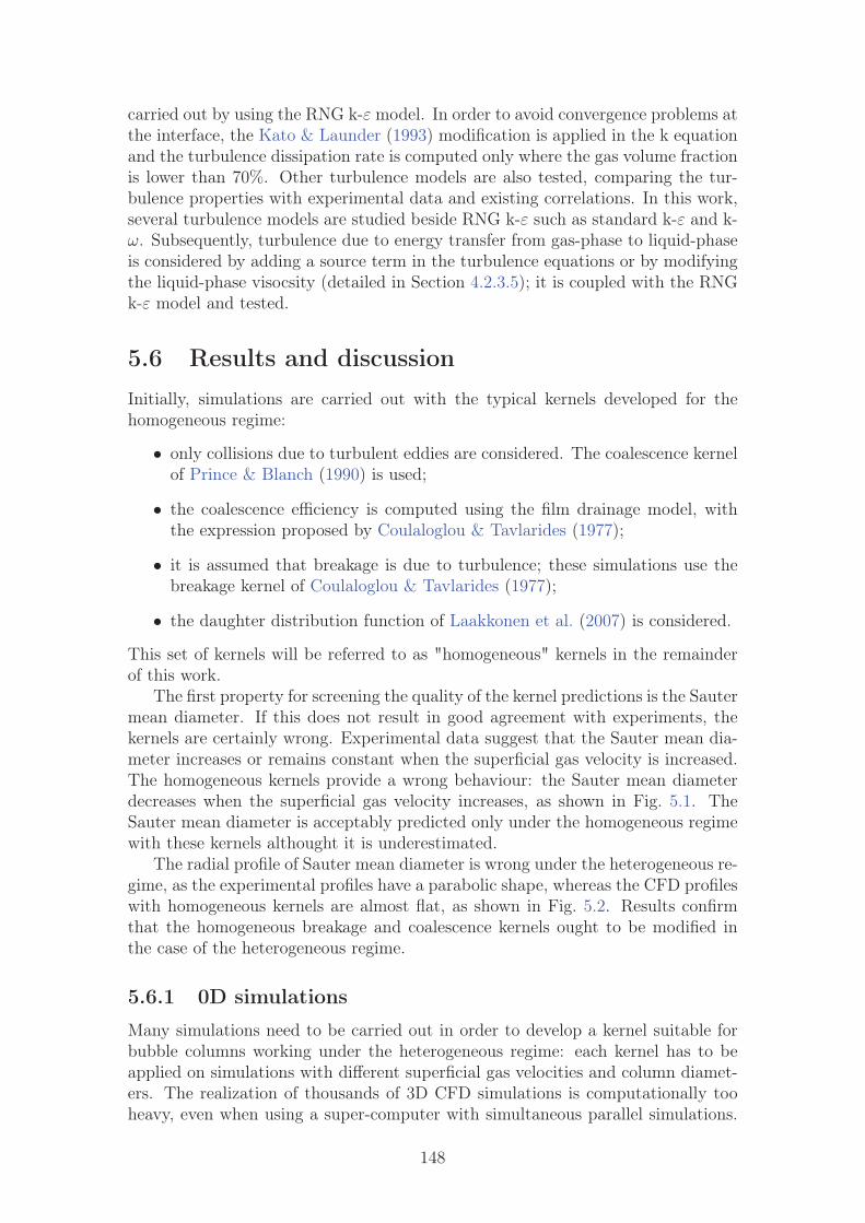
carried out by using the RNG k-ε model. In order to avoid convergence problems atthe interface, the Kato & Launder (1993) modification is applied in the k equationand the turbulence dissipation rate is computed only where the gas volume fractionis lower than 70%. Other turbulence models are also tested, comparing the tur-bulence properties with experimental data and existing correlations. In this work,several turbulence models are studied beside RNG k-ε such as standard k-ε and k-ω. Subsequently, turbulence due to energy transfer from gas-phase to liquid-phaseis considered by adding a source term in the turbulence equations or by modifyingthe liquid-phase visocsity (detailed in Section 4.2.3.5); it is coupled with the RNGk-ε model and tested.
5.6 Results and discussionInitially, simulations are carried out with the typical kernels developed for thehomogeneous regime:
• only collisions due to turbulent eddies are considered. The coalescence kernelof Prince & Blanch (1990) is used;
• the coalescence efficiency is computed using the film drainage model, withthe expression proposed by Coulaloglou & Tavlarides (1977);
• it is assumed that breakage is due to turbulence; these simulations use thebreakage kernel of Coulaloglou & Tavlarides (1977);
• the daughter distribution function of Laakkonen et al. (2007) is considered.
This set of kernels will be referred to as "homogeneous" kernels in the remainderof this work.
The first property for screening the quality of the kernel predictions is the Sautermean diameter. If this does not result in good agreement with experiments, thekernels are certainly wrong. Experimental data suggest that the Sauter mean dia-meter increases or remains constant when the superficial gas velocity is increased.The homogeneous kernels provide a wrong behaviour: the Sauter mean diameterdecreases when the superficial gas velocity increases, as shown in Fig. 5.1. TheSauter mean diameter is acceptably predicted only under the homogeneous regimewith these kernels althought it is underestimated.
The radial profile of Sauter mean diameter is wrong under the heterogeneous re-gime, as the experimental profiles have a parabolic shape, whereas the CFD profileswith homogeneous kernels are almost flat, as shown in Fig. 5.2. Results confirmthat the homogeneous breakage and coalescence kernels ought to be modified inthe case of the heterogeneous regime.
5.6.1 0D simulations
Many simulations need to be carried out in order to develop a kernel suitable forbubble columns working under the heterogeneous regime: each kernel has to beapplied on simulations with different superficial gas velocities and column diamet-ers. The realization of thousands of 3D CFD simulations is computationally tooheavy, even when using a super-computer with simultaneous parallel simulations.
148
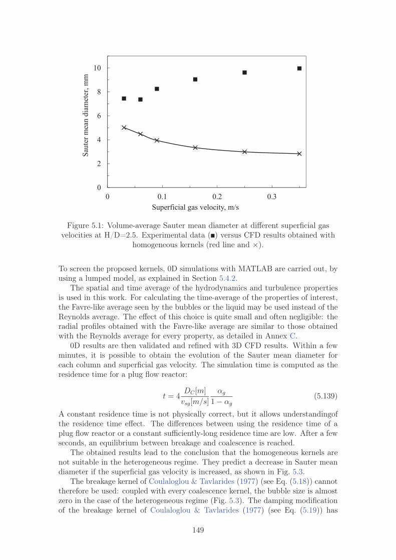
0
2
4
6
8
10
0 0.1 0.2 0.3Superficial gas velocity, m/s
Saut
er m
ean
diam
eter
, mm
Figure 5.1: Volume-average Sauter mean diameter at different superficial gasvelocities at H/D=2.5. Experimental data (�) versus CFD results obtained with
homogeneous kernels (red line and ×).
To screen the proposed kernels, 0D simulations with MATLAB are carried out, byusing a lumped model, as explained in Section 5.4.2.
The spatial and time average of the hydrodynamics and turbulence propertiesis used in this work. For calculating the time-average of the properties of interest,the Favre-like average seen by the bubbles or the liquid may be used instead of theReynolds average. The effect of this choice is quite small and often negligible: theradial profiles obtained with the Favre-like average are similar to those obtainedwith the Reynolds average for every property, as detailed in Annex C.
0D results are then validated and refined with 3D CFD results. Within a fewminutes, it is possible to obtain the evolution of the Sauter mean diameter foreach column and superficial gas velocity. The simulation time is computed as theresidence time for a plug flow reactor:
t = 4DC [m]
vsg[m/s]
αg
1− αg
(5.139)
A constant residence time is not physically correct, but it allows understandingofthe residence time effect. The differences between using the residence time of aplug flow reactor or a constant sufficiently-long residence time are low. After a fewseconds, an equilibrium between breakage and coalescence is reached.
The obtained results lead to the conclusion that the homogeneous kernels arenot suitable in the heterogeneous regime. They predict a decrease in Sauter meandiameter if the superficial gas velocity is increased, as shown in Fig. 5.3.
The breakage kernel of Coulaloglou & Tavlarides (1977) (see Eq. (5.18)) cannottherefore be used: coupled with every coalescence kernel, the bubble size is almostzero in the case of the heterogeneous regime (Fig. 5.3). The damping modificationof the breakage kernel of Coulaloglou & Tavlarides (1977) (see Eq. (5.19)) has
149

0
2
4
6
8
0 0.25 0.5 0.75 1
Saut
er m
ean
diam
eter
, mm
Radial position(a) 0.03 m/s.
0
2
4
6
8
10
0 0.25 0.5 0.75 1
Saut
er m
ean
diam
eter
, mm
Radial position
(b) 0.16 m/s.
Figure 5.2: Sauter mean diameter profile in the case of homogeneous (0.03 m/s)and heterogeneous (0.16 m/s) flow regimes at H/D=2.5. Experimental data (�)
versus CFD results obtained with homogeneous kernels (dashed line).
150

0
2
4
6
8
10
0 0.1 0.2 0.3Superficial gas velocity, m/s
Saut
er m
ean
diam
eter
, mm
Figure 5.3: Averaged Sauter mean diameter at different superficial velocities with0D simulations: experimental data (�) versus 0D simulations with the breakagekernels of Coulaloglou & Tavlarides (1977) (dashed line and �), Coulaloglou &Tavlarides (1977) with damping effect (dotted line and ×) and Laakkonen et al.
(2007) (solid line and �) coupled with the homogeneous coalescence kernels.
very little effect. The bubble size obtained with the breakage kernel of Laakkonenet al. (2007) is slightly better, but still not acceptable if coupled with homogeneouscoalescence kernels.
In 0D simulations the coalescence and breakage kernels can be studied separ-ately in order to understand the source of mismatch with the observed experimentaldata. Closer observation of the simulation data reveal that the problem is the co-alescence kernel that predict zero coalescence resulting in a decrease of the Sautermean diameter when the superficial gas velocity increases. These results confirmthat the coalescence kernel ought to be modified. The efficiency of Coulaloglou &Tavlarides (1977) is not suitable for the heterogeneous regime, in fact the turbulentdissipation rate is too high and the coalescence efficiency is almost zero for high ε.Every coalescence efficiency obtained with the film drainage model is not suitable:the Sauter mean diameter decreases if the superficial gas velocity grows (Fig. 5.4).Therefore another model, more properly describing the phenomena involved duringbubble coalescence under the heterogeneous regime, must be used.
The critical approach velocity model proposed by Lehr et al. (2002) is thentested. This coalescence kernel provides a correct behaviour for the Sauter meandiameter: it increases with the superficial gas velocity, but the values are incorrect,as shown in Fig. 5.5. This kernel looks interesting, but the constants have tobe modified and more accurate kernel constants can be obtained with 3D CFDsimulations.
151

0
0.1
0.2
0.3
0.4
0 0.1 0.2 0.3
Superficial gas velocity, m/s
Saut
er m
ean
diam
eter
, mm
Figure 5.4: Averaged Sauter mean diameter at different superficial velocitiesobtained with 0D simulations without breakage (only coalescence obtained withthe film drainage model), starting with an initial bubble size equal to 0.1 mm
(solid line and �).
0
10
20
30
0 0.1 0.2 0.3Superficial gas velocity, m/s
Saut
er m
ean
diam
eter
, mm
Figure 5.5: Averaged Sauter mean diameter at different superficial velocities with0D simulations: experimental data (�) versus 0D simulations with the collision
frequency of Lehr et al. (2002), the coalescence efficiency of Lehr et al. (2002) andthe breakage kernel of Laakkonen et al. (2007) (solid line and ×).
152

5.6.2 Kernel parameter identification with 3D CFD simula-tions
Several combinations of breakage and coalescence kernels are studied. Differentmodels for the breakage kernel, collision frequency and coalescence efficiency aretested, while the daughter distribution function of Laakkonen et al. (2007) is used,because of its analytical solution. 0D simulation results allow excluding the co-alescence efficiency kernels based on the film drainage model. Nevertheless, somesimulations by using the film drainage model are carried out in order to validatethe 0D simulations.
As detailed at the beginning of Chapter 5.6, "homogeneous" kernels cannotbe used in the case of bubble columns under the heterogeneous regime. Breakageand coalescence phenomena can be studied separately to understand the causesof discrepancy. The coalescence kernel predicts a Sauter mean diameter decreasewhen the superficial gas velocity increases, as shown in Fig. 5.6. As reported above
0
2
4
6
8
10
0 0.1 0.2 0.3Superficial gas velocity, m/s
Saut
er m
ean
diam
eter
, mm
Figure 5.6: Sauter mean diameter at different superficial gas velocities:experimental data (�) versus CFD results obtained with homogeneous kernels(dashed line and ×), with film drainage velocity model and Laakkonen et al.
(2006) breakage (dash-dot line and �), with film drainage model withoutbreakage (dotted line and �) and with the critical approach velocity model and
the Laakkonen et al. (2006) breakage kernel (solid line and �).
in 0D simulations, coalescence efficiency of Coulaloglou & Tavlarides (1977) cannotbe used in the case of heterogeneous regime. The turbulent dissipation rate is toohigh and the coalescence efficiency decreases too much for high turbulent dissipationrates. The kernels of coalescence efficiency based on the film drainage model are notsuitable, as the Sauter mean diameter decreases when the superficial gas velocityincreases (Fig. 5.6). These results confirm that the film drainage model does notwell describe the heterogeneous flow regime, in accordance with 0D simulations.The Sauter mean diameter profiles should be parabolic, whereas the CFD profiles
153

with homogeneous kernels are completely flat for every operating condition, asshown in Fig. 5.7. In order to further validate these results, some correctionsfor high gas volume fractions are proposed. The breakage kernel of Coulaloglou& Tavlarides (1977) with damping effect (Eq. (5.19)), coalescence efficiency ofWang et al. (2005b) (Eq. (5.58)) and Coulaloglou & Tavlarides (1977) for high gasfraction (Eq. (5.81)) have been tested. These corrections are not enough to obtainacceptable results if they are used with a film drainage model coalescence efficiency.
The breakage kernel of Coulaloglou & Tavlarides (1977) with damping effect,reported in Eq. (5.19), cannot be used: the Sauter mean diameter is too low forboth the homogeneous and heterogeneous regimes. By using the breakage kernelproposed by Laakkonen et al. (2007), the results are in a better agreement withexperiments. As detailed above, the breakage kernel of Laakkonen et al. (2007)could provide realistic results if coupled with a correct coalescence kernel.
The critical approach velocity model of Lehr et al. (2002) is then tested. Thecritical approach velocity model results in a correct trend for the Sauter meandiameter, that increases with the superficial gas velocity, although the numericalabsolute values are not exact. This kernel seems interesting but it is necessary tomodify the constants.
The objective is to obtain a model with a wider range of validity, suitable underdifferent operating conditions, with a focus on the heterogeneous regime. Underthe heterogeneous regime, the best results seem to be obtained by coupling thecollision frequency of Wang et al. (2005b), the coalescence efficiency of Lehr et al.(2002), the breakage kernel of Laakkonen et al. (2006) and the daughter distributionfunction of Laakkonen et al. (2007).
The critical approach velocity is equal to 0.08 m/s for pure water. The criticalapproach velocity has a lower value for tap water (contaminated water). Withthe collision frequency of Wang et al. (2005b), the bubble size increases with thesuperficial gas velocity but its values are higher than in the experiments. As sug-gested by Buffo (2012), the constant
√2π/4 should be replaced with an empirical
constant that can be fitted with CFD simulations. This set of kernels provides aspace-averaged Sauter mean diameter that slightly increases with the superficialgas velocity and its values are similar to experimental data if a constant equal to0.16 is used, as demonstrated in Fig. 5.6.
The Sauter mean diameter profiles obtained with this model are compared withthe experimental data in Fig. 5.7 for different operating conditions. The radialprofiles of Sauter mean diameter are well-predicted. CFD and experimental profilesare in a good agreement. The Sauter mean diameter profile is parabolic in caseof heterogeneous regime. These profiles are quite correct for every superficial gasvelocity. The main discrepancies appear next to the wall. The profile is almost flatfor a superficial gas velocity equal to 0.03 m/s, that corresponds to the homogeneousregime. These preliminary results are in accordance with the experiments and theymust be validated by analysing the effects of turbulence, initial conditions andscale-up.
The film drainage model cannot be used in the case of heterogeneous regime,as the turbulence dissipation rate is too high. It causes a contact time than is toolow compared with the film drainage time and thus the efficiency is almost zero.The critical approach velocity model does not consider contact and drainage time,but the relative velocity between two colliding bubbles and then the efficiency is
154

02468
10
0 0.25 0.5 0.75 1Radial position
(a) 0.03 m/s
02468
10
0 0.25 0.5 0.75 1Radial position
(b) 0.06 m/s
02468
10
0 0.25 0.5 0.75 1Radial position
(c) 0.09 m/s
02468
10
0 0.25 0.5 0.75 1Radial position
(d) 0.16 m/s
02468
10
0 0.25 0.5 0.75 1Radial position
(e) 0.25 m/s
02468
10
0 0.25 0.5 0.75 1Radial position
(f) 0.35 m/s
Figure 5.7: Sauter mean diameter profile at different superficial gas velocities atH/D=2.5. Experimental data (�) versus CFD results obtained with critical
approach velocity model and Laakkonen et al. (2006) breakage.
155

not zero in the case of heterogeneous regime. If two bubbles approach at a velocitylower than the critical one, they coalesce also under the heterogeneous regime. Thecritical approach velocity model is used in the following part of this work.
5.6.3 CFD-PBM simulations validation
5.6.3.1 Hydrodynamics validation
The hydrodynamics was well-predicted using a fixed bubble size, as detailed inChapter 4. CFD-PBM coupling allows to understand if the swarm factor proposedin the previous chapter can be used also for poly-disperse systems. The drag lawcan be modified in order to consider the effect of bubble size distribution as follows:
FD ≈ 3
4
αgρlρg
|urel|urel
∫L2 CD (L) n dL∫
L3 n dL
≈ 3
4
αgρlρg
|urel|urel
∑3i=1 wiL
2i CD (L)∑3
i=1 wiL3i
. (5.140)
With the operating conditions investigated in this work, the minimum value used inEq. (4.58) ought to be increased (hmin=0.3). The presence of small and big bubblesincreases the risk of huge accumulation of bubbles. The value of hmin here proposedcan be used both with a fixed bubble size (without PBM) and with a PBM. For thebiggest columns, i.e. φ 1 m and φ 3 m, the classical value of hmin=0.15 can be usedand then this value can be considered as suitable for industrial purposes. Since withthe column φ 0.4 m, with hmin=0.15 and in presence of a PBM, big accumulationsof bubbles occur for high gas volume fractions, a value of 0.30 is used in thischapter. The choice of this value influences only the CFD hydrodynamics for veryhigh superficial gas velocities, i.e. equal to 0.25 m/s and 0.35 m/s, while the effectis lower in the other cases.
CFD-PBM simulations using the default drag force and the drag force presentedin Eq. (5.140) are compared in the case of the heterogeneous regime. The effect ofthe modification of the drag force is low, as observed in Fig. 5.8. It can be due tothe fact that the terminal velocity is almost constant in this size range (Gemelloet al. (2018b)). This drag force correction is robust and the computational time isnot affected. This effect could be important under presence of a class of bubblessmaller than 2 mm or bigger than 10 mm. The CFD-PBM global hydrodynamics iscorrect, as observed by Gemello et al. (2018b) without PBM: gas gold-up, local gasfraction (Fig. 5.8a) and liquid velocity (Fig. 5.8b) are similar to the experimentalresults. The swarm factor proposed by Gemello et al. (2018b) and detailed inChapter 4 can be considered as valid for poly-disperse systems.
5.6.4 Turbulence model effects
The turbulence properties (i.e. turbulent viscosity, turbulence kinetic energy andturbulence dissipation rate) influence the coalescence and breakage kernels. Inparticular, the turbulence dissipation rate plays a direct role in the coalescenceand breakage kernels. The simulations presented before are carried out by usingthe RNG k-ε model. Other turbulence models ought to be tested, comparingthe turbulence properties with experimental data and existing correlations. In
156
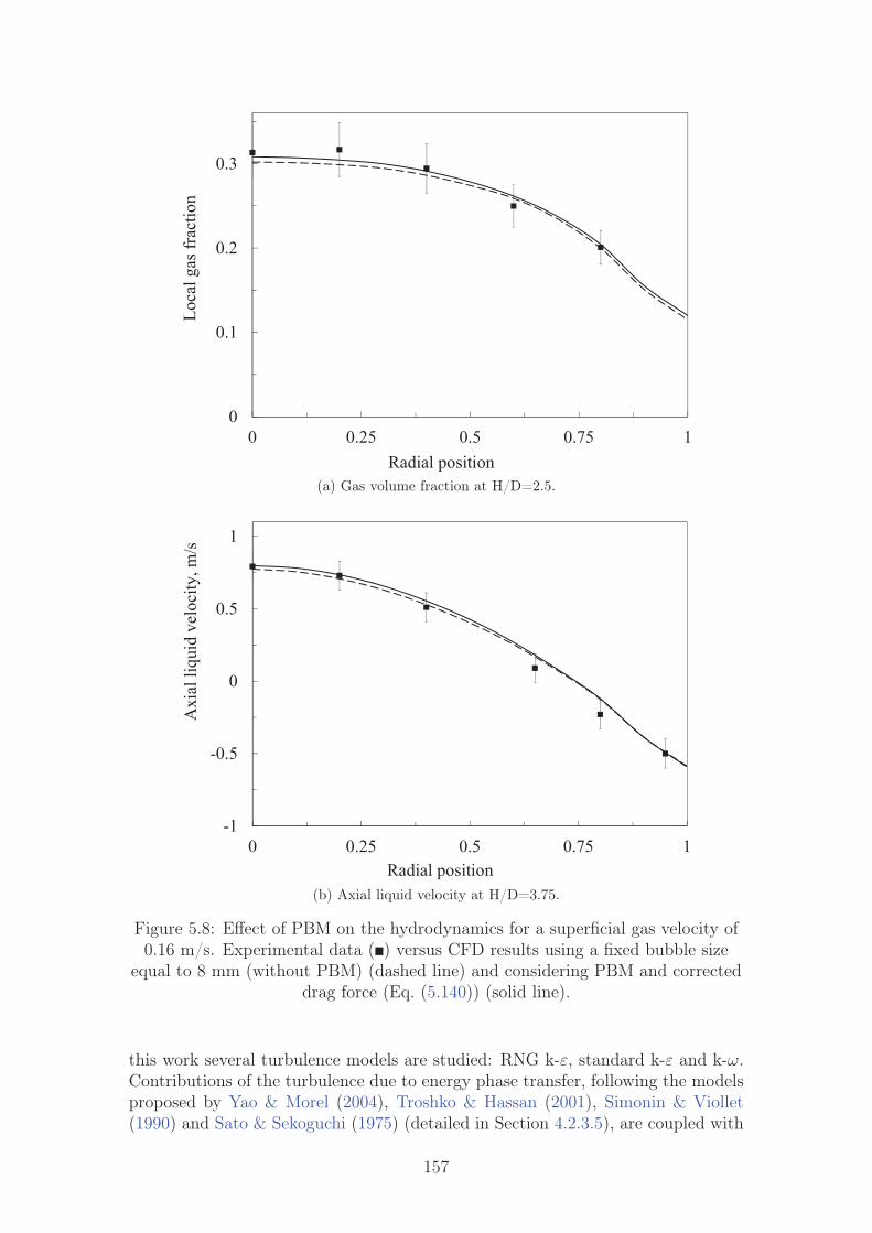
0
0.1
0.2
0.3
0 0.25 0.5 0.75 1Radial position
Loca
l gas
frac
tion
(a) Gas volume fraction at H/D=2.5.
-1
-0.5
0
0.5
1
0 0.25 0.5 0.75 1Radial position
Axi
al li
quid
vel
ocity
, m/s
(b) Axial liquid velocity at H/D=3.75.
Figure 5.8: Effect of PBM on the hydrodynamics for a superficial gas velocity of0.16 m/s. Experimental data (�) versus CFD results using a fixed bubble size
equal to 8 mm (without PBM) (dashed line) and considering PBM and correcteddrag force (Eq. (5.140)) (solid line).
this work several turbulence models are studied: RNG k-ε, standard k-ε and k-ω.Contributions of the turbulence due to energy phase transfer, following the modelsproposed by Yao & Morel (2004), Troshko & Hassan (2001), Simonin & Viollet(1990) and Sato & Sekoguchi (1975) (detailed in Section 4.2.3.5), are coupled with
157

the RNG k-ε model and tested.Forret (2003) studied the turbulent viscosity in bubble columns in a wide range
of operating conditions. She proposed a correlation for the calculation of the tur-bulent viscosity in the column centre:
νt = 0.036D1.6v0.11sg . (5.141)
Furthermore, Forret (2003) studied its radial profile. The radial profile should beflat until a normalized radial position of 0.8 and then decrease quickly to zero atthe wall (see Fig. 5.9).
0
0.005
0.01
0.015
0 0.2 0.4 0.6 0.8 1
Effe
ctiv
e ki
nem
atic
visc
osity
, m2 /s
Radial position
Figure 5.9: Kinematic turbulent viscosity for the column φ 0.4 m with asuperficial gas velocity equal to 0.16 m/s at H/D=2.5. Data obtained by Forret(2003) (�) versus CFD results with different turbulence models: RNG k-ε (blacksolid line), standard k-ε (black dashed line), realizable k-ε (black dotted line),
standard k-ω (red solid line) and SST k-ω (red dashed line).
The standard k-ω model provides turbulent viscosity value closer to the correl-ation, but a wrong radial profile in the case of heterogeneous regime. The RNGk-ε model underestimates the turbulent viscosity, while the realizable k-ε modeloverestimates it. The standard k-ε model strongly overestimates it. These resultsare compared in Fig. 5.9.
In Chapter 4, different kinematic turbulent viscosity have been tested and com-pred with CFD results, as shown in Fig. 4.20. The best agreement was obtainedwith the correlation of Kawase & Moo-Young (1989), while higher discrepanciesappear with the correlations of Miyauchi & Shyu (1970) and Burns & Rice (1997).By using the the correlation of Kawase & Moo-Young (1989), the RNG k-ε modelseems to provide the best results. The choice of the kinematic turbulent viscositycorrelation influences the comparison between the turbulence models.
The turbulence kinetic energy can be calculated using the fluctuating liquidvelocity components:
k =1
2
((u′)2 + (v′)2 + (w′)2
). (5.142)
158
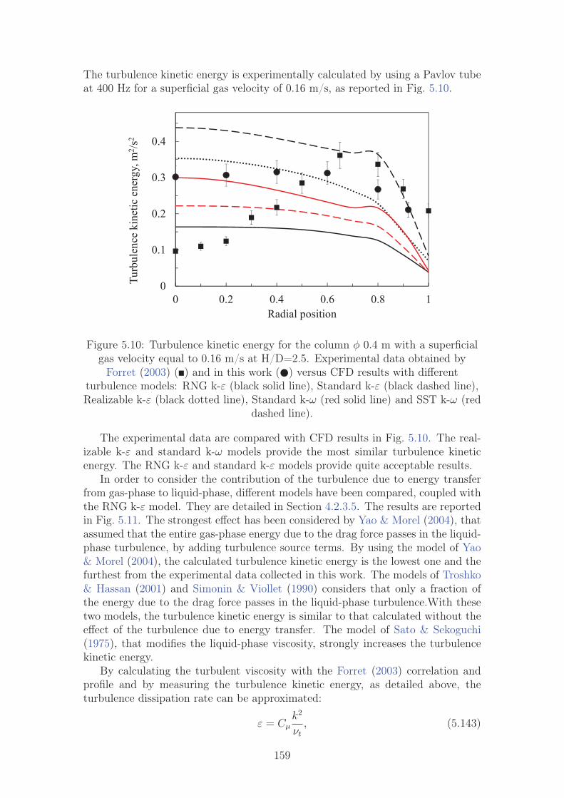
The turbulence kinetic energy is experimentally calculated by using a Pavlov tubeat 400 Hz for a superficial gas velocity of 0.16 m/s, as reported in Fig. 5.10.
0
0.1
0.2
0.3
0.4
0 0.2 0.4 0.6 0.8 1
Turb
ulen
ce k
inet
ic e
nerg
y, m
2 /s2
Radial position
Figure 5.10: Turbulence kinetic energy for the column φ 0.4 m with a superficialgas velocity equal to 0.16 m/s at H/D=2.5. Experimental data obtained by
Forret (2003) (�) and in this work (�) versus CFD results with differentturbulence models: RNG k-ε (black solid line), Standard k-ε (black dashed line),Realizable k-ε (black dotted line), Standard k-ω (red solid line) and SST k-ω (red
dashed line).
The experimental data are compared with CFD results in Fig. 5.10. The real-izable k-ε and standard k-ω models provide the most similar turbulence kineticenergy. The RNG k-ε and standard k-ε models provide quite acceptable results.
In order to consider the contribution of the turbulence due to energy transferfrom gas-phase to liquid-phase, different models have been compared, coupled withthe RNG k-ε model. They are detailed in Section 4.2.3.5. The results are reportedin Fig. 5.11. The strongest effect has been considered by Yao & Morel (2004), thatassumed that the entire gas-phase energy due to the drag force passes in the liquid-phase turbulence, by adding turbulence source terms. By using the model of Yao& Morel (2004), the calculated turbulence kinetic energy is the lowest one and thefurthest from the experimental data collected in this work. The models of Troshko& Hassan (2001) and Simonin & Viollet (1990) considers that only a fraction ofthe energy due to the drag force passes in the liquid-phase turbulence.With thesetwo models, the turbulence kinetic energy is similar to that calculated without theeffect of the turbulence due to energy transfer. The model of Sato & Sekoguchi(1975), that modifies the liquid-phase viscosity, strongly increases the turbulencekinetic energy.
By calculating the turbulent viscosity with the Forret (2003) correlation andprofile and by measuring the turbulence kinetic energy, as detailed above, theturbulence dissipation rate can be approximated:
ε = Cμk2
νt, (5.143)
159

0
0.1
0.2
0.3
0.4
0 0.2 0.4 0.6 0.8 1
Turb
ulen
ce k
inet
ic e
nerg
y, m
2 /s2
Radial position
Figure 5.11: Turbulence kinetic energy for the column φ 0.4 m with a superficialgas velocity equal to 0.16 m/s at H/D=2.5. Experimental data obtained in this
work (�) versus CFD results with RNG k-ε model (solid line) coupled withdifferent models for considering the turbulence due to energy transfer from
gas-phase to liquid-phase: Yao & Morel (2004) (dotted line), Troshko & Hassan(2001) (dash-dot-dot line), Simonin & Viollet (1990) (dash-dot line) and Sato &
Sekoguchi (1975) (dashed line).
where Cμ is a numerical constant approximately equal to 0.09 in many cases andequal to 0.085 in ANSYS Fluent.
Every turbulence model underestimates the turbulence dissipation rate. Thestandard k-ε and standard k-ω models slightly underestimate the turbulence dissip-ation rate, while the discrepancies are higher with the other models. All the othermodels have turbulence dissipation rate values smaller than the experimental oneof about 20-40%. These results are reported in Fig 5.12.
Power consumption per unit of mass should equal to the loss of potential energyper unit of mass, i.e. the turbulence dissipation rate considering an energy balance.The power consumption per unit of volume (P/V ) can be calculated with thefollowing formula (Roels & Heijnen 1980, Menzel et al. 1990):
P/V =1
Hpusg ln
(1 + ρl
g H (1− αg)
p
), (5.144)
where H is the operating liquid height, p is the external pressure, usg is the super-ficial gas velocity, ρl is the density of the liquid phase, g is the gravity accelerationand αg is the global gas volume fraction.
Considering a superficial gas velocity equal to 0.16 m/s, with a global gas volumefraction equal to 0.24, the turbulence dissipation rate should be equal to 1.08 m2/s3,slightly bigger than the values presented in Fig. 5.12.
The contribution of the turbulence due to energy transfer from gas-phase toliquid-phase on the turbulence dissipation rate is presented in Fig 5.13. Everymodel tested in this work has a positive effect on the turbulence dissipation rate:
160

0
0.25
0.5
0.75
1
1.25
0 0.2 0.4 0.6 0.8 1
Turb
ulen
ce d
issip
atio
n ra
te, m
2 /s3
Radial position
Figure 5.12: Turbulence dissipation rate for the column φ 0.4 m with a superficialgas velocity equal to 0.16 m/s at H/D=2.5. Data obtained with Eq. (5.143) (�)versus CFD results with different turbulence models: RNG k-ε (black solid line),Standard k-ε (black dashed line), Realizable k-ε (black dotted line), Standard k-ω
(red solid line) and SST k-ω (red dashed line).
it is higher than the one calculated without considering the turbulence due tothe energy transfer. The results are more similar to the data calculated withEq. (5.143).
The turbulence properties comparison strongly depends on the turbulent vis-cosity correlation choice. The standard k-ω model seems to be the best choice ifthe the turbulent viscosity is calculated with the Forret (2003) correlation, whilethe RNG k-ε model seems to be the best one if the turbulent viscosity correlationproposed by Kawase & Moo-Young (1989) is adopted. The contribution of theturbulence due to energy transfer from gas-phase to liquid-phase has a positiveeffect on the turbulence dissipation rate, while the effect on the turbulence kineticenergy strongly depends on the model that is adopted.
The objective of this part of the work is not to compare the turbulent propertiesor to suggest a better turbulence model, but understand the effect that turbulentproperties have on coalescence and breakage. The effect of the turbulence modelchoice on the Sauter mean diameter is quite low, as shown in Fig. 5.14. Every tur-bulence models provides similar results. The standard k-ε presents some differencesnext to the wall, with a more pronounced profile. The effect of the turbulence dueto energy transfer from gas-phase to liquid-phase on the Sauter mean diameter islow (Fig. 5.15).
It is possible to conclude that the coalescence and breakage kernels studiedin this work are suitable for many turbulence models and the best results areobtained with the RNG k-ε, realizable k-ε and standard k-ω and SST k-ω models.This set of kernel can be used also if the turbulence due to energy transfer fromgas to liquid is considered. One possible explanation is that using the criticalapproach velocity model, the effect of the turbulence dissipation rate on the coalesce
161

0
0.5
1
1.5
0 0.2 0.4 0.6 0.8 1Turb
ulen
ce d
issip
atio
n ra
te, m
2 /s3
Radial position
Figure 5.13: Turbulence dissipation rate for the column φ 0.4 m with a superficialgas velocity equal to 0.16 m/s at H/D=2.5. Data obtained with Eq. (5.143) (�)
versus CFD results with RNG k-ε model (solid line) coupled with differentmodels for considering the turbulence due to energy transfer from gas-phase to
liquid-phase: Yao & Morel (2004) (dotted line), Troshko & Hassan (2001)(dash-dot-dot line), Simonin & Viollet (1990) (dash-dot line) and Sato &
Sekoguchi (1975) (dashed line).
0
2
4
6
8
10
0 0.2 0.4 0.6 0.8 1
Saut
er m
ean
diam
eter
, mm
Radial position
Figure 5.14: Sauter mean diameter for the column φ 0.4 m with a superficial gasvelocity equal to 0.16 m/s at H/D=2.5. Experimental data obtained by Gemelloet al. (2018a) (�) versus CFD results with different turbulence models: RNG k-ε(black solid line), Standard k-ε (black dashed line), Realizable k-ε (black dotted
line), Standard k-ω (red solid line) and SST k-ω (red dashed line).
162
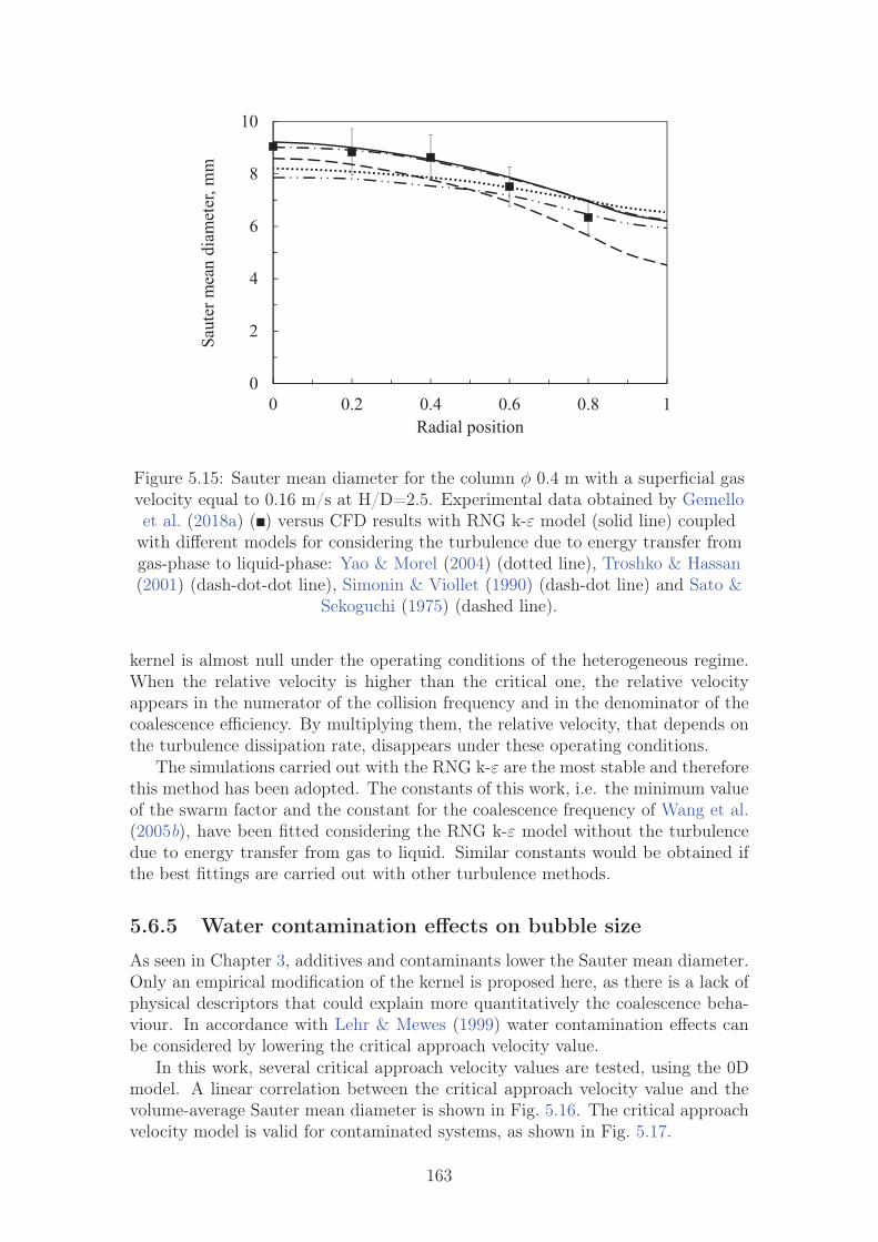
0
2
4
6
8
10
0 0.2 0.4 0.6 0.8 1
Saut
er m
ean
diam
eter
, mm
Radial position
Figure 5.15: Sauter mean diameter for the column φ 0.4 m with a superficial gasvelocity equal to 0.16 m/s at H/D=2.5. Experimental data obtained by Gemelloet al. (2018a) (�) versus CFD results with RNG k-ε model (solid line) coupled
with different models for considering the turbulence due to energy transfer fromgas-phase to liquid-phase: Yao & Morel (2004) (dotted line), Troshko & Hassan(2001) (dash-dot-dot line), Simonin & Viollet (1990) (dash-dot line) and Sato &
Sekoguchi (1975) (dashed line).
kernel is almost null under the operating conditions of the heterogeneous regime.When the relative velocity is higher than the critical one, the relative velocityappears in the numerator of the collision frequency and in the denominator of thecoalescence efficiency. By multiplying them, the relative velocity, that depends onthe turbulence dissipation rate, disappears under these operating conditions.
The simulations carried out with the RNG k-ε are the most stable and thereforethis method has been adopted. The constants of this work, i.e. the minimum valueof the swarm factor and the constant for the coalescence frequency of Wang et al.(2005b), have been fitted considering the RNG k-ε model without the turbulencedue to energy transfer from gas to liquid. Similar constants would be obtained ifthe best fittings are carried out with other turbulence methods.
5.6.5 Water contamination effects on bubble size
As seen in Chapter 3, additives and contaminants lower the Sauter mean diameter.Only an empirical modification of the kernel is proposed here, as there is a lack ofphysical descriptors that could explain more quantitatively the coalescence beha-viour. In accordance with Lehr & Mewes (1999) water contamination effects canbe considered by lowering the critical approach velocity value.
In this work, several critical approach velocity values are tested, using the 0Dmodel. A linear correlation between the critical approach velocity value and thevolume-average Sauter mean diameter is shown in Fig. 5.16. The critical approachvelocity model is valid for contaminated systems, as shown in Fig. 5.17.
163

0
2
4
6
0 0.04 0.08Critical approach velocity, m/s
Saut
er m
ean
diam
eter
, mm
Figure 5.16: Effect of the critical approach velocity value on the Sauter meandiameter with a superficial gas velocity equal to 0.16 m/s.
0
2
4
6
8
10
0 0.25 0.5 0.75 1Radial position
Saut
er m
ean
diam
eter
, mm
Figure 5.17: Ethanol effect on the Sauter mean diameter with a superficial gasvelocity equal to 0.16 m/s. Experimental data obtained by Gemello et al. (2018a)with demineralised water (�), ethanol 0.01% (�) and ethanol 0.05% (�) versusCFD results with different critical approach velocities: 0.08 m/s (demineralised
water) (solid line), 0.065 m/s (ethanol 0.01%) (dashed line) and 0.05 m/s(ethanol 0.05%) (dotted line).
By knowing the space-averaged Sauter mean diameter, it is possible to obtainthe critical approach velocity model and this value can be used to study the Sauter
164
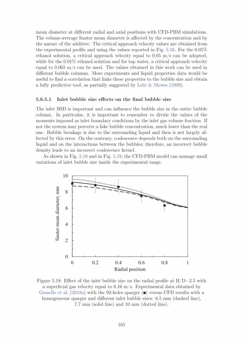
mean diameter at different radial and axial positions with CFD-PBM simulations.The volume-average Sauter mean diameter is affected by the concentration and bythe nature of the additive. The critical approach velocity values are obtained fromthe experimental profile and using the values reported in Fig. 5.16. For the 0.05%ethanol solution, a critical approach velocity equal to 0.05 m/s can be adopted,while for the 0.01% ethanol solution and for tap water, a critical approach velocityequal to 0.065 m/s can be used. The values obtained in this work can be used indifferent bubble columns. More experiments and liquid properties data would beuseful to find a correlation that links these properties to the bubble size and obtaina fully predictive tool, as partially suggested by Lehr & Mewes (1999).
5.6.5.1 Inlet bubble size effects on the final bubble size
The inlet BSD is important and can influence the bubble size in the entire bubblecolumn. In particular, it is important to remember to divide the values of themoments imposed as inlet boundary conditions by the inlet gas volume fraction. Ifnot the system may perceive a fake bubble concentration, much lower than the realone. Bubble breakage is due to the surrounding liquid and then is not largely af-fected by this error. On the contrary, coalescence depends both on the surroundingliquid and on the interactions between the bubbles; therefore, an incorrect bubbledensity leads to an incorrect coalescence kernel.
As shown in Fig. 5.18 and in Fig. 5.19, the CFD-PBM model can manage smallvariations of inlet bubble size inside the experimental range.
0
2
4
6
8
10
0 0.2 0.4 0.6 0.8 1
Saut
er m
ean
diam
eter
, mm
Radial position
Figure 5.18: Effect of the inlet bubble size on the radial profile at H/D=2.5 witha superficial gas velocity equal to 0.16 m/s. Experimental data obtained by
Gemello et al. (2018a) with the 92-holes sparger (�) versus CFD results with ahomogeneous sparger and different inlet bubble sizes: 6.5 mm (dashed line),
7.7 mm (solid line) and 10 mm (dotted line).
165

0
2
4
6
8
10
0 1 2 3 4
Saut
er m
ean
diam
eter
, mm
Axial position (H/D)
Figure 5.19: Effect of the inlet bubble size on the axial profile at the centre of thecolumn with a superficial gas velocity equal to 0.16 m/s. Experimental dataobtained by Gemello et al. (2018a) with the 92-holes sparger (�) versus CFDresults with a homogeneous sparger and different inlet bubble sizes: 6.5 mm
(dashed line), 7.7 mm (solid line) and 10 mm (dotted line).
By using an initial bubble size slightly lower than the previous one, equal to6.5 mm, the bubble size is almost the same above a height of 1 m. By using aninitial bubble size equal to 10 mm, the bubble size is slightly higher, but it is stillacceptable. Small variations of initial bubble size are not very important, as thesystem reaches an equilibrium between coalescence and breakage.
5.6.5.2 Sparger effects on the bubble size
Gemello et al. (2018a) realized experiments with two different spargers. Firstly, aperforated sparger with several small holes (2 mm) is used. It generates bubbleswith a Sauter mean diameter between 5 mm and 10 mm. The profile close to thebottom is almost flat, as detailed in Chapter 3. A sparger with 7 holes of 9 mm isthen used, in order to modify the inlet bubble size. It causes the formation of bigbubbles close to the bottom of the column, above the holes. The sparger choiceradically influences the bubble dimension in the lowest part of the column. Aperforated sparger with big holes causes the formation of big bubbles in the lowestpart of the column, above the holes. The breakage of the bubbles is the predominantphenomenon if big bubbles are present. The bubble size decreases quickly alongthe axial position and the bubbles are almost not affected by the sparger after somecentimetres. They reach quickly the equilibrium bubble dimension.
The previous simulations were realized by considering the high number of holesof the first sparger (92 holes) as a homogeneous porous plate. In CFD-PBM simu-lations, the gas enters the column already mixed with the liquid. A constant inletgas volume fraction is assumed. The initial Sauter mean diameter is fixed equal
166
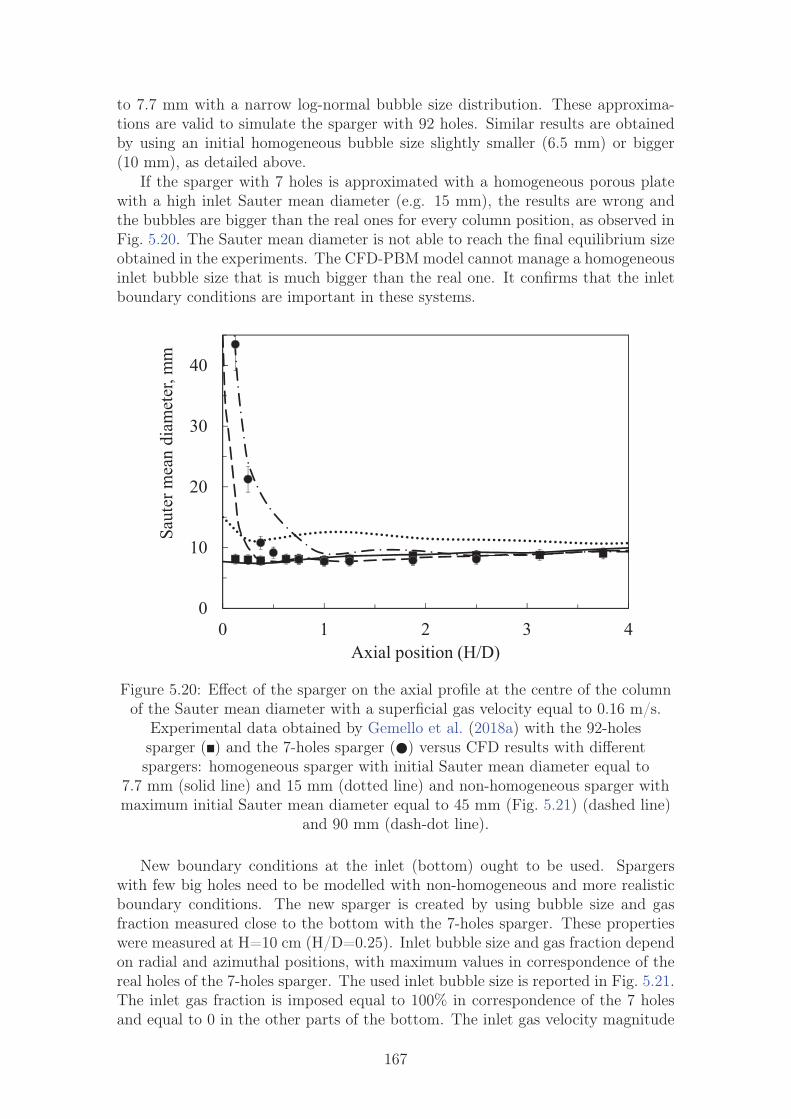
to 7.7 mm with a narrow log-normal bubble size distribution. These approxima-tions are valid to simulate the sparger with 92 holes. Similar results are obtainedby using an initial homogeneous bubble size slightly smaller (6.5 mm) or bigger(10 mm), as detailed above.
If the sparger with 7 holes is approximated with a homogeneous porous platewith a high inlet Sauter mean diameter (e.g. 15 mm), the results are wrong andthe bubbles are bigger than the real ones for every column position, as observed inFig. 5.20. The Sauter mean diameter is not able to reach the final equilibrium sizeobtained in the experiments. The CFD-PBM model cannot manage a homogeneousinlet bubble size that is much bigger than the real one. It confirms that the inletboundary conditions are important in these systems.
0
10
20
30
40
0 1 2 3 4
Saut
er m
ean
diam
eter
, mm
Axial position (H/D)
Figure 5.20: Effect of the sparger on the axial profile at the centre of the columnof the Sauter mean diameter with a superficial gas velocity equal to 0.16 m/s.
Experimental data obtained by Gemello et al. (2018a) with the 92-holessparger (�) and the 7-holes sparger (�) versus CFD results with differentspargers: homogeneous sparger with initial Sauter mean diameter equal to
7.7 mm (solid line) and 15 mm (dotted line) and non-homogeneous sparger withmaximum initial Sauter mean diameter equal to 45 mm (Fig. 5.21) (dashed line)
and 90 mm (dash-dot line).
New boundary conditions at the inlet (bottom) ought to be used. Spargerswith few big holes need to be modelled with non-homogeneous and more realisticboundary conditions. The new sparger is created by using bubble size and gasfraction measured close to the bottom with the 7-holes sparger. These propertieswere measured at H=10 cm (H/D=0.25). Inlet bubble size and gas fraction dependon radial and azimuthal positions, with maximum values in correspondence of thereal holes of the 7-holes sparger. The used inlet bubble size is reported in Fig. 5.21.The inlet gas fraction is imposed equal to 100% in correspondence of the 7 holesand equal to 0 in the other parts of the bottom. The inlet gas velocity magnitude
167

is calculated in order to obtain a correct superficial gas velocity (iterative method),and it depends on the imposed inlet gas fraction and on the used interpolationmethod.
50
40
30
20
10
0
Saut
er m
ean
diam
eter
, mm
Figure 5.21: Inlet Sauter mean diameter with the 7-holes sparger.
The effect of the 7-holes sparger is important close to the bottom, in CFD-PBMsimulations (Fig. 5.20). With this sparger, big bubbles appear close to the bottom.These big bubbles disappear quickly and the sparger effect is almost null above1 m. The behaviour is in good agreement with the experimental data. In CFD-PBM simulations, the equilibrium size is reached a little slower, but the agreementis still good. An important aspect is that, in the CFD simulations, the turbulencedissipation rate is low next to the sparger. It might be used to study more in detailthe turbulence models, with a focus on the turbulence properties in the lowest partof the column. A study on the effects of the inlet turbulence properties would beuseful to further validate the kernels proposed in this work.
Considering these results, the effects of breakage and coalescence can be par-tially decoupled. Close to the bottom, the breakage is the main phenomenon andthe coalescence is negligible. In this region, where the breakage is the principalphenomenon, the bubble size behaviour is quite correct, as the Sauter mean dia-meter decreases quickly, in good agreement with the experimental data. If both thebreakage kernel and the final equilibrium bubble size are correct, the coalescencemodel can be considered as correct. Breakage and coalescence kernels are validover a wide range of conditions.
168

5.6.6 Scale-up effects
Raimundo (2015) collected experimental data with tap water by using bubblecolumns at different scales: the column diameters were equal to 0.15 m, 0.4 m,1 m and 3 m. The Sauter mean diameter does not change too much when thecolumn diameter changes. It may be assumed that the behaviour is the same withdemineralised water.
The initial rhomboidal cooper mesh with 40,000 cells, obtained and used withthe column φ 0.4 m, is scaled up, in order to analyse the scale-up effect on theSauter mean diameter in the CFD-PBM simulations. Grid-independent tests arerequired and they confirm that this mesh can be used for scale-up purposes, asreported in Chapter 4.
In the CFD-PBM simulations, the Sauter mean diameter is approximately thesame also if the column diameter changes (Fig. 5.22). CFD-PBM results are quitein accordance with the experimental data of Raimundo (2015). Similar results areobtained by using RNG k-ε and k-ω turbulence models, as shown in Fig. 5.22. Itmeans that the breakage and coalescence kernels proposed above can be used forthe scale-up of these systems, with different turbulence models.
The final goal of this work is the industrial scale-up of bubble columns under theheterogeneous flow regime. Industrially, the Sauter mean diameter is not known apriori and it is often difficult to obtain it. The four bubble columns are simulatedusing different homogeneous inlet bubble sizes. The inlet Sauter mean diameter hasan important effect with the smallest bubble columns. As presented in Fig. 5.23, theinlet bubble size partially influences the Sauter mean diameter at H/D=2.5 for thecolumn φ 0.4 m, while its influence is almost zero for the columns φ 1 m and φ 3 m.The time needed for one bubble to reach H/D=2.5 is longer in the biggest columnsthan in the smallest ones. It allows reaching the equilibrium bubble size with awider range of inlet Sauter mean diameters. The Sauter mean diameter obtainedwith the CFD simulations are compared with the experimental data presented inChapter 3, that was obtained with demineralised water in the column φ 0.4 m(Fig. 5.23). New experiments by using bubble columns at different scales shouldbe carried out in order to improve these models. Fortunately, industrial bubblecolumns are usually large and it means that the lack of knowledge about the bubblesize close to the bottom does not strongly influence the final Sauter mean diameter.
5.7 Conclusions and perspectives
CFD simulations are frequently used for the study of bubble columns under indus-trial operating conditions and bubble size plays a key role in the hydrodynamicsand transport phenomena for these systems. CFD simulations are coupled witha population balance model (PBM) in order to consider coalescence and breakagephenomena.
Coalescence and breakage phenomena are caused by different mechanisms andthe most important are linked to turbulent fluctuations in the continuous phase.Breakage causes the formation of daughter bubbles and it is then necessary todefine both the breakage frequency (breakage kernel) and the daughter distributionfunction. Coalescence rate is instead quantified by a kernel in turn divided into twoparts: a collision frequency and a coalescence efficiency. The collision frequency
169

0
2
4
6
8
10
0 0.2 0.4 0.6 0.8 1
Saut
er m
ean
diam
eter
, mm
Radial position
(a) RNG k-ε model.
0
2
4
6
8
10
0 0.2 0.4 0.6 0.8 1
Saut
er m
ean
diam
eter
, mm
Radial position
(b) Standard k-ω model.
Figure 5.22: Scale-up effect with a superficial gas velocity equal to 0.16 m/s anddifferent turbulence models on the radial profile of Sauter mean diameter at
H/D=2.5. Experimental data obtained by Gemello et al. (2018a) on the columnφ 0.4 m (�) versus CFD results with different bubble column: φ 0.4 m (solid
lines), φ 1 m (dashed lines) and φ 3 m (dotted lines).
170

0
2
4
6
8
10
0 0.2 0.4 0.6 0.8 1
Saut
er m
ean
diam
eter
, mm
Radial position
(a) φ 0.4 m
0
2
4
6
8
10
0 0.25 0.5 0.75 1
Saut
er m
ean
diam
eter
, mm
Radial position
(b) φ 1 m
0
2
4
6
8
10
0 0.25 0.5 0.75 1
Saut
er m
ean
diam
eter
, mm
Radial position
(c) φ 3 m
Figure 5.23: Effect of inlet bubble size (homogeneous sparger) for different bubblecolumns with a superficial gas velocity equal to 0.16 m/s on the radial profile of
Sauter mean diameter at H/D=2.5. Experimental data obtained by Gemello et al.(2018a) on the column φ 0.4 m (�) versus CFD results with different inlet bubble
sizes: 6.5 mm (dashed lines), 7.7 mm (solid lines) and 10 mm (dotted lines).
171

defines the number of collisions while the coalescence efficiency is the fraction ofcolliding bubbles that actually coalesce. The latter one can be studied by usingdifferent methods: film drainage model, energy model and critical approach velocitymodel. The film drainage model is the most used for the homogeneous regime. Thework of this chapter suggests that the critical approach velocity model is the bestone for the heterogeneous regime. The best breakage kernels and the collisionfrequency need to be coupled with the critical approach velocity model. The meanbubble Sauter mean diameter predicted by the model in good agreement withthe experiments for both the homogeneous and the heterogeneous flow regimes ifthe kernels are correctly fitted. Its radial profile has a parabolic shape under theheterogeneous regime, while it is almost flat under the homogeneous regime.
The best set of breakage and coalescence kernels in the case of heterogeneousregime seems to be the breakage kernel proposed by Laakkonen et al. (2006), thedaughter distribution function proposed by Laakkonen et al. (2007), the modi-fied collision frequency proposed by Wang et al. (2005b) and the critical approachvelocity model for coalescence efficiency proposed by Lehr et al. (2002). Theseequations are reported here:
• Breakage kernel - Laakkonen et al. (2006)
g(L) = c3ε1/3 erfc
(√c4
σ
ρlε2/3L5/3+ c5
μl√ρlρgε1/3L4/3
),
with c3 = 4.0, c4 = 0.04 and c5 = 0.01.
• Daughter distribution function - Laakkonen et al. (2007)
bki =3240Lk
i
(k + 9)(k + 12)(k + 15).
• Collision frequency - Wang et al. (2005b)
h0 (L1, L2) = C ′2 γ Π(L1 + L2)
2 ε1/3√
L2/31 + L
2/32 ,
where C ′2 = 0.16, while Π and γ are two correction factors:
– Wu et al. (1998), Π =
[1− exp
(−CΠ
α1/3maxα
1/3g
α1/3max − α
1/3g
)], with CΠ = 3;
– Wang et al. (2005b), γ =αmax
αmax − αg
, with αmax = 0.8.
• Coalescence efficiency - Lehr et al. (2002)
λ (L1, L2) = min
(ucrit
urel
, 1
),
with ucrit=0.08 m/s for demineralised water, lower for contaminated systems.
172

Coalescence and breakage kernels are generally affected by turbulence properties.Many turbulence models are tested: their effect on the bubble size seems fairlysmall. The coalescence and breakage kernels proposed in this chapter can be usedwith many turbulence models involved in Eulerian-Eulerian simulations. The con-tribution of the turbulence due to the energy transfer from the gas-phase to theliquid-phase is still an open question and it affects the turbulence properties. Itseffects on the bubble size is low, if the set of coalescence and breakage kernels pro-posed in work is used. This set of kernels is suitable for several turbulence modelsand even if the turbulence due to the energy transfer is considered.
The previous set of kernels has been obtained, under the heterogeneous regime,with demineralised water using a homogeneous gas sparger. It is also valid forless-coalescent liquids, i.e. contaminated water and ethanol solutions. Contamin-ants and additives effects can be considered with an adjusted value of the criticalapproach velocity. CFD-PBM simulations well predict hydrodynamics and bubblesize for these systems. More experiments with additives and experimental dataon the liquid properties are required to obtain a fully predictive tool, that con-siders the additive effects a priori. The link between liquid physical properties andcoalescence needs to be clarified.
The CFD-PBM simulations with this set of kernels are not very sensitive tothe inlet bubble size. The results are in agreement with the experiments obtainedby using the sparger with many small holes. On the other hand, these simulationscannot consider an inlet bubble size much larger than the experimental one. Theinlet boundary conditions are important. It is necessary to model the sparger withfew big holes with non-homogeneous and realistic inlet boundary conditions. Inthis work, the sparger with few big holes is modelled using the experimental gasfraction and bubble size measured in the lowest part of the column. It allows thecorrect prediction of hydrodynamics and bubble size for this sparger.
The proposed set of kernels seems to be suitable also for the industrial scale-upof bubble columns under the heterogeneous regime, but more studies and experi-mental data are required.
173

Bibliography
Alopaeus, V., Koskinen, J., Keskinen, K. I. & Majander, J. (2002), ‘Simulation ofthe population balances for liquid-liquid systems in a nonideal stirred tank. part2 - parameter fitting and the use of the multiblock model for dense dispersions’,Chemical Engineering Science 57(10), 1815–1825.
Andersson, B., Andersson, R., Håkansson, L., Mortensen, M., Sudiyo, R., Van Wa-chem, B. & Hellström, L. (2012), Computational Fluid Dynamics for Engineers,first edn, University Press, Cambridge, UK.
Bilicki, Z. & Kestin, J. (1987), ‘Transition criteria for two-phase flow patterns invertical upward flow.’, International Journal of Multiphase Flow 13, 283–298.
Buffo, A. (2012), Multivariate population balance for turbulent gas-liquid flows.,PhD thesis, Politecnico di Torino, Torino, Italy.
Buffo, A., De Bona, J., Vanni, M. & Marchisio, D. L. (2016), ‘Simplified volume-averaged models for liquid-liquid dispersions: Correct derivation and comparisonwith other approaches.’, Chemical Engineering Science 153, 382–393.
Buffo, A., Vanni, M., Marchisio, D. L. & Fox, R. O. (2013), ‘MultivariateQuadrature-Based Moments Methods for turbulent polydisperse gas-liquid sys-tems’, International Journal of Multiphase Flow 50, 41–57.
Burns, L. F. & Rice, R. G. (1997), ‘Circulation in bubble columns’, AmericanInstitute of Chemical Engineering Journal 43(6), 1390–1402.
Carrica, P. M. & Clausse, A. A. (1993), A Mathematical Description of the CriticalHeat Flux as Nonlinear Dynamic Instability, G. Gouesbet and A. Berlemont.Instabilities in Multiphase Flow, Plenum Press, New York.
Casamatta, G. & Vogelpohl, A. (1985), ‘Modeling of fluid dynamics and masstransfer in extraction columns’, German Chemical Engineering 8, 96–103.
Chesters, A. K. (1991), ‘The modeling of coalescence processes in fluid-liquid dis-persions: A review of current understanding’, Chemical Engineering Researchand Design: transactions of the Institution of Chemical Engineers: Part A69, 259–270.
Colella, D., Vinci, D., Bagatin, R., Masi, M. & Abu Bakr, E. (1999), ‘A study oncoalescence and breakage mechanisms in three different bubble columns’, Chem-ical Engineering Science 54(21), 4767–4777.
Colin, C., Riou, X. & Fabre, J. (2004), Turbulence and shear-induced coalescencein gas-liquid pipe flows, in ‘ICMF 2004 - 5th International Conference on Mul-tiphase Flow’, Yokohama, Japan.
Coulaloglou, C. A. (1975), Dispersed phase interactions in an agitated flow vessel,PhD thesis, Illinois Institute of Technology, Chicago, Illinois.
174
Coulaloglou, C. A. & Tavlarides, L. L. (1977), ‘Description of interaction processesin agitated liquid-liquid dispersions’, Chemical Engineering Science 32, 1289–1297.
De Bona, J., Buffo, A., Vanni, M. & Marchisio, D. L. (2016), ‘Limitations ofsimple mass transfer models in polydisperse liquid-liquid dispersions.’, ChemicalEngineering Journal 296, 112–121.
Dette, H. & Studden, W. J. (1997), The Theory of Canonical Moments with Ap-plications in Statistics, Probability, and Analysis., John Wiley and Sons., NewYork.
Doubliez, L. (1991), ‘The drainage and rupture of a non-foaming liquid film formedupon bubble impact with a free surface’, International Journal of MultiphaseFlow 17, 783–803.
Falzone, S., Buffo, A., Vanni, M. & Marchisio, D. L. (2018), ‘Simulation of turbulentcoalescence and breakage of bubbles and droplets in the presence of surfactants,salts, and contaminants’, Advances in Chemical Engineering 52, 125–188.
Forret, A. (2003), Hydrodynamics scale-up of slurry bubble columns., PhD thesis,Université Claude Bernard Lyon 1 - IFPEN, Lyon, France.
Frank, T., Zwart, P. J., Krepper, E., Prasser, H. M. & Lucas, D. (2008), ‘Validationof cfd models for mono- and polydisperse airâĂŞwater two-phase flows in pipes’,Nuclear Engineering and Design 238(3), 647–659.
Friedlander, S. K. (1977), Smoke, Dust and Haze, Wiley, New York.
Fu, X. Y. & Ishii, M. (2003), ‘Two-group interfacial area transport in vertical air-water flow: I. mechanistic model’, Nuclear Engineering and Design 219(2), 14–168.
Gao, Z., Li, D., Buffo, A., Podgórska, W. & Marchisio, D. L. (2016), ‘Simula-tion of droplet breakage in turbulent liquid-liquid dispersions with CFD-PBM:Comparison of breakage kernels’, Chemical Engineering Science 142, 277–288.
Gemello, L., Cappello, V., Augier, F., Marchisio, D. L. & Plais, C. (2018b), ‘CFD-based scale-up of hydrodynamics and mixing in bubble columns’, Chemical En-gineering Research and Design 136, 846–858.
Gemello, L., Plais, C., Augier, F., Cloupet, A. & Marchisio, D. L. (2018a), ‘Hy-drodynamics and bubble size in bubble columns: Effects of contaminants andspargers’, Chemical Engineering Science 184, 93–102.
Godin, F. B., Cooper, G., D. & Rey, A. D. (1999), ‘Numerical methods for apopulation-balance model of a periodic fermentation process.’, American Insti-tute of Chemical Engineering Journal 45, 1359–1364.
Gordon, R. G. (1981), ‘Error bounds in equilibrium statistical mechanics’, Journalof Mathematical Physics 9, 655–663.
175

Gunawan, R., Fusman, I. & Braatz, R. D. (2004), ‘High resolution algorithms formultidimensional population balance equations.’, American Institute of ChemicalEngineering Journal 50, 2738–2749.
Hesketh, R. P., Russell, T. W. F. & Etchells, A. W. (1987), ‘Bubble size in hori-zontal pipelines.’, American Institute of Chemical Engineering Journal 33, 663–667.
Hibiki, T. & Ishii, M. (2000), ‘One-group interfacial area transport of bubblyflows in vertical round tubes’, International Journal of Heat and Mass Transfer43, 2711–2726.
Hibiki, T., Takasama, T. & Ishii, M. (2001), ‘Interfacial area transport of bub-bly flow in a small diameter pipe’, Journal of Nuclear Science and Technology38, 614–620.
Howarth, W. J. (1964), ‘Coalescence of drops in a turbulent flow field’, ChemicalEngineering Science 19, 33–38.
Jeffreys, G. V. & Davies, G. A. (1971), Coalescence of Liquid Droplets and LiquidDispersion: Recent Advances in Liquid-Liquid Extraction, 1 st edn, PergamonPress, Oxford, UK.
Kalkach-Navarro, S., Lahey Jr., R. T. & Drew, D. A. (1994), ‘Analysis of thebubbly/slug flow regime transition’, Nuclear Engineering and Design 151(1), 15–39.
Kato, M. & Launder, B. E. (1993), The modeling of turbulent flow around sta-tionary and vibrating square cylinders, in ‘9th Symposium on Turbulent ShearFlows’, Kyoto, Japan.
Kawase, Y. & Moo-Young, M. (1989), ‘Turbulence intensity in bubble columns’,The Chemical Engineering Journal 40(1), 55–58.
Kennard, E. H. (1938), Kinetic Theory of Gases, McGraw-Hill, New York.
Kentish, S. E., Stevens, G. W. & Pratt, H. R. C. (1998), ‘Estimation of coalescenceand breakage rate constants within a kühni column’, Industrial & EngineeringChemistry Research 37(3), 1099–1106.
Konno, M., Muto, T. & Saito, S. (1988), ‘Coalescence of dispersed drops in anagitated tank’, Journal of Chemical Engineering of Japan 21, 335–338.
Kuboi, R., Komasawa, I. & Otake, T. (1972), ‘Collision and coalescence of disperseddrops in turbulent liquid flow’, Journal of Chemical Engineering of Japan 5, 423–424.
Kumar, J., Peglow, M., Warnecke, G. & Heinrich, S. (2008), ‘The cell average tech-nique for solving multi-dimensional aggregation population balance equations’,Computers & Chemical Engineering 32, 1810–1830.
Laakkonen, M., Alopaeus, V. & Aittamaa, J. (2006), ‘Validation of bubble break-age, coalescence and mass transfer models for gas-liquid dispersion in agitatedvessel’, Chemical Engineering Science 61, 218–228.
176

Laakkonen, M., Moilanen, P., Alopaeus, V. & Aittamaa, J. (2007), ‘Modellinglocal bubble size distributions in agitated vessels’, Chemical Engineering Science62, 721–740.
Lasheras, J. C., Eastwood, C., Martínez-Bazán, C. & Montañés, J. L. (2002), ‘Areview of statistical models for the break-up of an immiscible fluid immersedinto a fully developed turbulent flow’, International Journal of Multiphase Flow28, 247–278.
Lee, C. H., Erickson, L. E. & Glasgow, L. A. (1987), ‘Bubble break-up and co-alescence in turbulent gas-liquid dispersions’, Chemical Engineering Communic-ations 59, 65–84.
Lehr, F. & Mewes, D. (1999), ‘A transport equation for the interfacial area densityapplied to bubble columns’, Chemical Engineering Science 56, 1159–1166.
Lehr, F., Millies, M. & Mewes, D. (2002), ‘Bubble-size distributions and flowfields in bubble columns’, American Institute of Chemical Engineering Journal48(11), 2426–2443.
Levich, V. G. (1962), Physicochemical Hydrodynamics, Prentice Hall, EnglewoodCliffs, NJ.
Li, D., Gao, Z., Buffo, A., Podgórska, W. & Marchisio, D. L. (2017), ‘Dropletbreakage and coalescence in liquid-liquid dispersions: Comparison of differentkernels with EQMOM and QMOM’, American Institute of Chemical EngineeringJournal 63(6), 2293–2311.
Liao, Y. & Lucas, D. (2009), ‘A literature review of theoretical models for dropand bubble breakup in turbulent dispersions’, Chemical Engineering Science64, 3389–3406.
Liao, Y. & Lucas, D. (2010), ‘A literature review on mechanisms and models for thecoalescence process of fluid particles’, Chemical Engineering Science 65, 2851–2864.
Luo, H. (1993), Coalescence, breakup and liquid circulation in bubble column re-actors, PhD thesis, The Norwegian Institute of Technology, Trondheim, Norway.
Luo, H. & Svendsen, H. F. (1996), ‘Modeling and simulation of binary approach byenergy conservation analysis’, Chemical Engineering Communications 145, 145–153.
Marchisio, D. L. & Fox, R. O. (2013), Computational Models for PolydisperseParticulate and Multiphase Systems, Cambridge Series in Chemical Engineering,Cambridge University Press, Cambridge, UK.
Marchisio, D. L., Vigil, R. D. & Fox, R. O. (2003a), ‘Implementation of the quad-rature method of moments in CFD codes for aggregation-breakage problems’,Chemical Engineering Science 58, 3337–3351.
177

Marchisio, D. L., Vigil, R. D. & Fox, R. O. (2003b), ‘Quadrature method of mo-ments for aggregation-breakage processes’, Journal of Colloid and Interface Sci-ence 258, 322–334.
Mazzei, L., Marchisio, D. L. & Lettieri, P. (2012), ‘New quadrature-based momentmethod for the mixing of inert polydisperse fluidized powders in commercial cfdcodes.’, American Institute of Chemical Engineering Journal 58(10), 3054–3069.
McClure, D. D., Deligny, J., Kavanagh, J. M., Fletcher, D. F. & Barton, G. W.(2014), ‘Impact of surfactant chemistry on bubble column systems’, ChemicalEngineering & Technology 37(4), 652–658.
McClure, D. D., Kavanagh, J. M., Fletcher, D. F. & Barton, G. W. (2013), ‘De-velopment of a CFD model of bubble column bioreactors: Part one - a detailedexperimental study’, Chemical Engineering & Technology 36(12), 2065–2070.
McClure, D. D., Norris, H., Kavanagh, J. M., Fletcher, D. F. & Barton, G. W.(2015), ‘Towards a CFD model of bubble columns containing significant surfact-ant levels’, Chemical Engineering Science 127, 189–201.
McGraw, R. (1997), ‘Description of aerosol dynamics by the quadrature method ofmoments.’, Aerosol Science and Technology 27, 255–265.
Menzel, T., In der Weide, T., Staudacher, O., Wein, O. & Onken, U. (1990),‘Reynolds stress model for bubble column reactor’, Industrial & EngineeringChemistry Research 29(6), 988–994.
Miyauchi, T. & Shyu, C.-N. (1970), ‘Flow of fluid in gas bubble columns’, KagakuKogaku 34(9), 958–964.
Narasimhan, G., Ramakrishna, D. & Gupta, J. P. (1979), ‘A model for transitionalbreakage probability of droplets in agitated lean liquid-liquid dispersions’, Chem-ical Engineering Science 34, 257–265.
Nevers, N. & Wu, J. L. (1971), ‘Bubble coalescence in viscous fluids.’, AmericanInstitute of Chemical Engineering Journal 17, 182–186.
Park, J. Y. & Blair, L. M. (1975), ‘The effect of coalescence on drop size distributionin an agitated liquid-liquid dispersion’, Chemical Engineering Science 30, 1057–1064.
Petitti, M., Nasuti, A., Marchisio, D. L., Vanni, M., Baldi, G., Mancini, N. &Podenzani, F. (2010), ‘Bubble size distribution modeling in stirred gas-liquidreactors with QMOM augmented by a new correction algorithm.’, AmericanInstitute of Chemical Engineering Journal 56, 36–53.
Podgórska, W. & Marchisio, D. L. (2016), ‘Modeling of turbulent drop coales-cence in the presence of electrostatic forces’, Chemical Engineering Research andDesign 108, 30–41.
Prince, M. J. & Blanch, H. W. (1990), ‘Bubble coalescence and break-up in air-sparged bubble columns’, American Institute of Chemical Engineering Journal36, 1485–1499.
178

Raimundo, P. M. (2015), Analysis and modelization of local hydrodynamics inbubble columns, PhD thesis, Université Grenoble Alpes.
Renardy, Y., Cristini, V. & Li, J. (2002), ‘Drop fragment distributions under shearwith inertia’, International Journal of Multiphase Flow 28, 1125–1147.
Revankar, S. T. (2001), Coalescence and breakup of fluid particles in multi-phaseflow, in ‘ICMF 2001 - 4th International Conference on Multiphase Flow’, Ne-wOrleans, Louisiana, USA.
Roels, J. A. & Heijnen, J. J. (1980), ‘Power dissipation and heat production inbubble columns: Approach based on nonequilibrium thermodynamics’, Biotech-nology and Bioengineering 22(11), 2399–2404.
Sato, Y. & Sekoguchi, K. (1975), ‘Liquid velocity distribution in two-phase bubbleflow’, International Journal of Multiphase Flow 2(1), 79–95.
Shinnar, R. & Church, J. M. (1960), ‘Predicting particle size in agitated disper-sions’, Industrial and Engineering Chemistry 52, 253–256.
Simon, M. (2004), Koaleszenz von Tropfen und Tropfenschwärmen, PhD thesis,Teschinschen Universtität Kaiserslautern, Kaiserslautern, Germany.
Simonin, O. & Viollet, P. L. (1990), ‘Modeling of turbulent two-phase jets loadedwith discrete particles’, Phenomena in Multiphase Flows pp. 259–269.
Sovova, H. (1981), ‘Breakage and coalescence of drops in a batch stirred vessel - iicomparison of model and experiments’, Chemical Engineering Science 36, 1567–1573.
Tomiyama, A. (1998), ‘Struggle with computational bubble dynamics.’, MultiphaseScience and Technology 10(4), 369.
Troshko, A. A. & Hassan, Y. A. (2001), ‘A two-equation turbulence model ofturbulent bubbly flows’, International Journal of Multiphase Flow 27(11), 1965–2000.
Vanni, M. (2000), ‘Approximate population balance equation for aggregation-breakage processes’, International Journal of Multiphase Flow 221, 143–160.
Wang, T. F., Wang, J. F. & Jin, Y. (2003), ‘A novel theoretical breakup kernelfunction for bubbles/droplets in a turbulent flow’, Chemical Engineering Science58(20), 4629–4637.
Wang, T. F., Wang, J. F. & Jin, Y. (2004), ‘An efficient numerical algorithm for “anovel theoretical breakup kernel function of bubble/droplet in a turbulent flow”’,Chemical Engineering Science 59, 2593–2595.
Wang, T. F., Wang, J. F. & Jin, Y. (2005a), ‘Population balance model for gas-liquid flows: Influence of bubble coalescence and breakup models’, Industrial &Engineering Chemistry Research 44(11), 7540–7549.
179

Wang, T. F., Wang, J. F. & Jin, Y. (2005b), ‘Theoretical prediction of flow re-gime transition in bubble columns by the population balance model’, ChemicalEngineering Science 60, 6199–6209.
Wang, T., Wang, J. & Jin, Y. (2006), ‘A CFD-PBM coupled model for gas-liquidflows’, American Institute of Chemical Engineering Journal 52, 125–140.
Wheeler, J. C. (1974), ‘Modified moments and gaussian quadratures.’, Rocky Moun-tain Journal of Mathematics 4, 287–296.
Wilf, H. (1962), Mathematics for the Physical Sciences., John Wiley and Sons.,New York.
Wright, D. L. (2007), ‘Numerical advection of moments of the particle size distri-bution in eulerian models.’, Journal of Aerosol Science 38, 352–369.
Wright, H. & Ramkrishna, D. (1994), ‘Factors affecting coalescence frequency ofdroplets in a stirred liquid-liquid dispersion’, American Institute of ChemicalEngineering Journal 40, 767–776.
Wu, Q., Kim, S. & Ishii, M. (1998), ‘One-group interfacial area transport in verticalbubbly flow’, International Journal of Heat and Mass Transfer 41, 1103–1112.
Yao, W. & Morel, C. (2004), ‘Volumetric interfacial area prediction in upward bub-bly two-phase flow’, International Journal of Heat and Mass Transfer 47, 307–328.
Yuan, C. & Fox, R. O. (2011), ‘Conditional quadrature method of moments forkinetic equations.’, Journal of Computational Physics 230, 8216–8246.
Zhao, H., Maisels, A., Matsoukas, T. & Zheng, C. (2007), ‘Analysis of four Monte-Carlo methods for the solution of population balances in dispersed systems’,Powder Technology 173, 38–50.
180

Chapter 6
Concluding remarks and futureworks
The objective of this work is to correctly predict the bubble size distributions inbubble columns and to study breakage and coalescence under industrial operatingconditions, focusing the attention on the heterogeneous flow regime.
To study these phenomena, new experimental data is required. Under the het-erogeneous regime, the liquid recirculation is strong and the radial profiles of gasvolume fraction, liquid velocity and mean bubble size have a strong concavity. Thepresence of contaminants and additives in the continuous phase, namely water,(demineralized water, tap water and demineralised water with small quantities ofethanol) has a strong effect on bubble size and coalescence. Bubbles in demin-eralised water are significantly bigger than in tap water. The addition of smallquantities of ethanol into demineralised water greatly decreases the bubble size,delays regime transition and increases the gas volume fraction under the hetero-geneous flow regime. The presence of ethanol modifies the surface bubble mobilityand decreases bubble coalescence. The relevant physical properties, that causethese differences, still need to be identified. Surface tension is one of them, butits variation is not the only explanation for these differences and more studiesare required to understand the factors that prevent coalescence. The relationshipbetween the physical properties of liquids and coalescence kernels needs to be clari-fied. More experiments with additives and experimental data on the relevant liquidproperties can be useful to consider them in the coalescence and breakage kernelsand to obtain a fully predictive tool.
The sparger choice strongly influences the bubble size and the hydrodynamicsclose to the bottom. With a sparger perforated with big holes, there is an accumu-lation of big bubbles in the lowest part of the column, in which bubble breakageis the main phenomenon. The effects of ethanol and sparger were combined todecouple coalescence and breakage phenomena. The presence of additives almostdoes not influence breakage, while its effect is important on bubble coalescence, asthe surface mobility changes. For these reasons, in this thesis several experimentshave been carried out, that allow to study correctly Sauter mean diameter andhydrodynamic properties in a wide range of operating conditions under the hetero-geneous regime, in presence of contaminants and additives and by using differentperforated spargers.
181

The study of bubble size distributions (BSD) could be interesting, but the cross-correlation technique used in the present work is not able to measure the BSD, as itcalculates only the Sauter mean diameter. An interesting experimental perspectivecould be to couple a classical optical probe method for BSD, that currently is notsuitable for the heterogeneous regime, with a cross-correlation technique for Sautermean diameter, in order to rescale the BSD under the heterogeneous regime.
The experimental results are used to carry out 3D URANS (Unsteady Reynolds-averaged Navier-Stokes equations) CFD (Computational Fluid Dynamics) simula-tions and the main results of this validation can be summarized as follows:
• Bubble column reactors under the heterogeneous flow regime are dominatedby interfacial forces and the drag force is the most important. Hydrodynamicprofiles have a strong link with interfacial forces and turbulence. A drag lawsuitable for oblate bubbles, such as Tomiyama (1998), needs to be used. Thisshould be modified by considering a swarm factor, to incorporate the swarmeffect. It must decrease the drag force for high gas volume fractions. For veryhigh gas volume fractions, the swarm factor of Simonnet et al. (2008) causesconvergence issues and an incorrect instantaneous behaviour, with bubblesthat create unphysical huge accumulations of bubbles. By modifying theswarm factor of Simonnet et al. (2008), CFD hydrodynamics is in agreementwith experimental data. A minimum value is added to the swarm factor ofSimonnet et al. (2008). The radial profiles of gas volume fraction and phasesvelocity are well predicted. The scale-up effects on hydrodynamics are in-vestigated and it is possible to state that this swarm factor can be assumedsuitable for industrial scale-up purposes. These results allow predicting cor-rectly the hydrodynamics of bubble columns under the heterogeneous regime,in the case of fixed bubble size.
• Turbulence has strong effects on these systems. Different turbulence modelsare tested. An extra diffusion coefficient due to bubbles, as presented byAlméras et al. (2015) is considered, in order to simulate the dispersion of ascalar. The RNG k-ε turbulence model predicts turbulence properties andscalar mixing reasonably, with good agreement with experimental data. Theextra diffusion coefficient due to bubbles cannot be neglected for the smallestcolumn, as it has a significant effect on scalar mixing (about 15%), while it isnegligible in other cases. The main contribution is due to the Shear InducedTurbulence (SIT).
• CFD simulations coupled with a Population Balance Model (PBM) to predictthe bubble size distribution show that bubble size influences the hydrodynam-ics and the BSD is required to estimate the interfacial area and the local heatand mass transfer rate. Numerous mechanisms are involved in bubble coales-cence and breakage. The existing models of breakage (Liao & Lucas 2009)and coalescence (Liao & Lucas 2010), developed for the homogeneous regime,are tested under the heterogeneous regime. The coalescence kernel can be di-vided in collision frequency and coalescence efficiency. Breakage and collisionfrequency mechanisms are linked to turbulent fluctuations. The coalescenceefficiency can be studied through the film drainage model under the homo-geneous regime, while it is not suitable for the heterogeneous regime. The
182

best model under the heterogeneous regime seems to be the critical approachvelocity model. The breakage model of Laakkonen et al. (2006), the collisionfrequency model of Wang et al. (2005) with a modified constant and the crit-ical approach velocity model for coalescence efficiency of Lehr et al. (2002)are demonstrated in this work to be suitable for the heterogeneous regime.The Sauter mean diameter of the bubbles predicted with this set of modelsis in agreement with experimental data for both the homogeneous and theheterogeneous regimes. The radial profile of the Sauter mean diameter isparabolic under the heterogeneous regime and almost flat under the homo-geneous regime, in agreement with experiments. Hydrodynamics is still wellpredicted.
• Turbulence properties influence the coalescence and breakage kernels and,in particular, the turbulence dissipation rate plays a direct role. Testingdifferent turbulence models, it is possible to conclude that the set of kernelsproposed in this work can be used with different classical turbulence modelsinvolved in Eulerian-Eulerian simulations.
• The proposed set of kernels allows carrying out simulations that are ableto handle small changes in inlet bubble size. The CFD-PBM results arein agreement with experimental data obtained with the sparger formed byseveral small holes (homogeneous gas distribution). These simulations cannothandle a homogeneous inlet bubble size much higher than the experimentaldata. The sparger with a few big holes needs to be modelled with non-homogeneous and more realistic inlet boundary conditions. In this work,Experimental gas fraction and bubble size measured close to the bottom areused to model this sparger. Hydrodynamics and bubble size are well predictedby using realistic inlet boundary conditions.
• The set of kernels proposed in this work can be used for scale-up purposes, butmore experiments and CFD studies are necessary on this topic. Experimentaldata with demineralized water, with or without alcohol addition at largerscale can be useful to validate these CFD-PBM models for industrial scale-up. CFD simulations with different geometries and meshes of industrial-scalebubble columns should be carried out.
Some limits have not yet been overcome and different perspectives and future worksare possible:
• The swarm factor proposed in this work is able to correctly predict the hy-drodynamics, but it has the limit to be empirical. The original swarm factorof Simonnet et al. (2008) was obtained thanks to experimental data and thecorrection proposed in this work is obtained thanks to a CFD fitting. A the-oretical model might provide suitable results for different gas-liquid systems.Moreover, the study of secondary interfacial forces, that are not consideredin this work, could be an interesting perspective.
• More studies on the cntribution of the turbulence due to energy transfer fromgas-phase to liquid-phase could be an important perspective. A comparisonbetween the effects of these models and the effects of the extra diffusivitymodel of Alméras et al. (2015) should be carried out.
183

• The critical approach velocity model of Lehr et al. (2002) has the advantagethat it can be successfully applied to less coalescent systems (alcohol solu-tions). The effect of the additives can be considered with an adjusted criticalapproach velocity. But the relevant physical properties that cause coalescencediminution still need to be identified. Surface tension variation is too smallto justify the bubble size differences. The critical approach velocity modelshould be based on a more solid theoretical foundation. As detailed above,other experiments with additives and measurements of the liquid propertiesare required.
• Moreover, a theoretical basis and DNS simulations could be used to obtain afully predictive set of kernels.
The ultimate goal would be to obtain completely a-priori industrial CFD-PBMsimulations, without the need for experiments.
184

BibliographyAlméras, E., Risso, F., Roig, V., Cazin, S., Plais, C. & Augier, F. (2015), ‘Mixing
by bubble-induced turbulence’, Journal of Fluid Mechanics 776, 458–474.
Laakkonen, M., Alopaeus, V. & Aittamaa, J. (2006), ‘Validation of bubble break-age, coalescence and mass transfer models for gas-liquid dispersion in agitatedvessel’, Chemical Engineering Science 61, 218–228.
Lehr, F., Millies, M. & Mewes, D. (2002), ‘Bubble-size distributions and flowfields in bubble columns’, American Institute of Chemical Engineering Journal48(11), 2426–2443.
Liao, Y. & Lucas, D. (2009), ‘A literature review of theoretical models for dropand bubble breakup in turbulent dispersions.’, Chemical Engineering Science64, 3389–3406.
Liao, Y. & Lucas, D. (2010), ‘A literature review on mechanisms and models for thecoalescence process of fluid particles.’, Chemical Engineering Science 65, 2851–2864.
Simonnet, M., Gentric, C., Olmos, E. & Midoux, N. (2008), ‘CFD simulation of theflow field in a bubble column reactor: Importance of the drag force formulationto describe regime transitions’, Chemical Engineering and Processing: ProcessIntensification 47(9), 1726–1737.
Tomiyama, A. (1998), ‘Struggle with computational bubble dynamics.’, MultiphaseScience and Technology 10(4), 369.
Wang, T. F., Wang, J. F. & Jin, Y. (2005), ‘Theoretical prediction of flow re-gime transition in bubble columns by the population balance model’, ChemicalEngineering Science 60, 6199–6209.
185

186

Appendix A
Experimental data
Superficial gasvelocity, m/s
Global gas volume fraction, %
DMW Tap water Ethanol 0.01% Ethanol 0.05%
0.01 3.50 3.50 3.15 3.500.02 7.69 6.96 6.72 8.220.03 10.78 10.93 10.98 12.490.04 12.73 13.34 13.54 16.690.05 14.83 15.23 15.37 19.630.06 15.50 16.72 17.13 21.790.07 16.61 18.94 18.94 23.260.08 18.10 20.15 20.15 25.270.09 18.93 20.17 21.41 26.650.10 19.75 20.25 22.37 27.970.11 20.94 21.44 23.49 29.250.12 21.52 22.02 23.86 30.340.13 22.29 22.79 25.11 31.390.14 23.00 23.72 26.32 32.260.15 23.70 25.31 27.10 32.980.16 24.60 26.02 27.44 33.540.17 25.00 26.37 28.26 34.640.18 25.55 26.55 29.44 35.170.20 26.74 27.74 29.77 36.350.22 27.41 27.91 31.15 38.220.24 28.39 28.39 31.76 39.640.25 28.86 28.86 32.64 40.170.26 29.18 29.68 33.22 40.670.28 30.11 30.61 33.80 41.460.30 30.72 31.72 34.92 42.230.32 31.46 32.46 36.00 42.890.35 33.18 34.18 37.08 45.12
Table A.1: Global hold-up for demineralised water (DMW), tap water, ethanol0.01% and ethanol 0.05% for the column φ 0.4 m.
187

Radialposition
Local gas volume fraction, %
0.03 m/s 0.06 m/s 0.09 m/s 0.16 m/s 0.25 m/s 0.35 m/s
0.00 12.99 21.07 25.01 31.32 38.36 46.090.20 12.89 21.16 24.51 31.65 39.42 45.230.40 12.07 20.88 22.16 29.43 36.21 41.390.60 12.54 20.80 19.08 24.98 29.76 36.290.80 12.37 18.62 16.99 20.07 24.04 29.42
Table A.2: Local gas volume fraction at H/D=2.5 with demineralised water.
Radialposition
Local gas volume fraction, %
0.03 m/s 0.06 m/s 0.09 m/s 0.16 m/s 0.25 m/s 0.35 m/s
0.00 12.6 21.5 23.4 30.7 37.7 43.00.20 13.0 20.5 22.8 30.0 34.1 43.40.40 12.2 20.0 22.4 27.7 34.1 42.00.60 12.3 20.5 20.5 25.6 30.4 36.20.80 12.2 19.0 15.8 20.8 23.7 26.6
Table A.3: Local gas volume fraction at H/D=2.5 with tap water.
Radialposition
Local gas volume fraction, %
0.03 m/s 0.06 m/s 0.09 m/s 0.16 m/s 0.25 m/s 0.35 m/s
0.00 12.95 22.75 26.90 34.06 40.50 48.000.20 12.70 22.38 26.66 34.05 41.50 46.600.40 12.26 22.46 24.64 31.48 38.20 43.500.60 12.30 22.44 21.54 27.06 32.00 38.000.80 12.23 20.58 18.80 22.19 26.00 31.00
Table A.4: Local gas volume fraction at H/D=2.5 with ethanol 0.01%.
Radialposition
Local gas volume fraction, %
0.03 m/s 0.06 m/s 0.09 m/s 0.16 m/s 0.25 m/s 0.35 m/s
0.00 12.88 26.12 29.73 37.43 43.65 51.230.20 12.33 24.81 29.89 36.14 44.60 48.680.40 12.65 25.62 28.37 33.65 39.15 46.540.60 11.82 25.71 25.23 29.57 33.05 40.100.80 11.95 24.50 21.50 23.31 28.15 33.40
Table A.5: Local gas volume fraction at H/D=2.5 with ethanol 0.05%.
188

Axialposition
Local gas volume fraction, %
DMW Tap water Ethanol 0.05%
0.125 10.350.25 9.1 9.2 9.530.375 9.01 9.1 9.060.5 9.71 9.8 10.21
0.625 10.270.75 10.83 10.5 10.831 10.83 11 11.33
1.25 11.65348 11.5 12.041.875 12.27 12.15 12.772.5 12.6 12.7 12.88
3.125 12.6 12.75 13.043.75 13 13.02 13.12
Table A.6: Local gas volume fraction at the column centre at different axialpositions with a superficial gas velocity equal to 3 cm/s (homogeneous regime)
with demineralised water (DMW), tap water and ethanol 0.05%.
Axialposition
Local gas volume fraction, %
DMW Tap water Ethanol 0.05%
0.125 29.21 30.3 30.680.25 28.7 29.52 30.670.375 28.175 28.87 31.240.5 27.63 28.765 31.61
0.625 27.63 28.010.75 27.64 28.31 32.21 27.63 28.4 31.95
1.25 28.385 28.735 32.651.875 28.735 30.455 34.162.5 30.7 31.335 37.43
3.125 31.44 37.753.75 32.3 34.015 39.34
Table A.7: Local gas volume fraction at the column centre at different axialpositions with a superficial gas velocity equal to 16 cm/s (heterogeneous regime)
with demineralised water (DMW), tap water and ethanol 0.05%.
189

Radialposition
Axial liquid velocity, m/s
0.03 m/s 0.06 m/s 0.09 m/s 0.16 m/s
0.00 0.20 0.51 0.81 0.880.20 0.15 0.49 0.67 0.660.40 0.18 0.38 0.41 0.500.60 0.14 0.28 0.24 0.230.75 0.12 -0.02 -0.10 -0.120.80 -0.06 -0.28 -0.28 -0.270.90 -0.18 -0.43 -0.46 -0.440.95 -0.35 -0.56 -0.59 -0.66
Table A.8: Axial liquid velocity at H/D=2.5 with demineralised water.
Radialposition
Axial liquid velocity, m/s
DMW Tap water Ethanol 0.05%
0.00 0.87 1.00 1.060.20 0.75 0.87 0.930.40 0.55 0.58 0.600.60 0.25 0.28 0.290.75 -0.130.80 -0.28 -0.35 -0.460.90 -0.480.95 -0.73 -0.49 -0.59
Table A.9: Axial liquid velocity at H/D=2.5 with a superficial gas velocity equalto 16 cm/s (heterogeneous regime) with demineralised water (DMW), tap water
and ethanol 0.05%.
190

Radialposition
Sauter mean diameter, mm
0.03 m/s 0.06 m/s 0.09 m/s 0.16 m/s 0.25 m/s 0.35 m/s
0.00 7.45 7.36 8.25 9.05 9.62 9.960.20 7.22 7.35 8.10 8.84 9.23 9.550.40 7.18 7.38 7.49 8.63 8.35 8.750.60 7.13 6.90 6.60 7.51 7.70 8.300.80 7.02 6.60 6.00 6.34 6.17 6.69
Table A.10: Sauter mean diameter at H/D=2.5 with demineralised water.
Radialposition
Sauter mean diameter, mm
0.03 m/s 0.09 m/s 0.16 m/s 0.25 m/s 0.35 m/s
0.00 5.68 6.74 7.11 7.41 7.620.20 5.58 6.24 6.97 7.53 8.070.40 6.38 5.87 6.83 7.22 7.490.60 5.56 5.54 5.67 6.17 6.060.80 5.33 4.35 4.07 4.76 5.14
Table A.11: Sauter mean diameter at H/D=2.5 with tap water.
Radialposition
Sauter mean diameter, mm
0.03 m/s 0.06 m/s 0.09 m/s 0.16 m/s 0.25 m/s 0.35 m/s
0.00 6.61 6.80 7.07 7.34 8.01 8.410.20 6.52 6.78 7.00 7.23 7.99 7.790.40 6.61 6.60 6.49 6.72 7.02 7.820.60 6.59 6.21 5.78 6.04 6.53 7.010.80 6.40 6.10 5.25 5.29 5.52 5.38
Table A.12: Sauter mean diameter at H/D=2.5 with ethanol 0.01%.
Radialposition
Sauter mean diameter, mm
0.03 m/s 0.06 m/s 0.09 m/s 0.16 m/s 0.25 m/s 0.35 m/s
0.00 5.83 5.85 5.88 6.07 6.66 6.920.20 5.98 5.85 5.83 5.99 6.78 6.760.40 6.01 5.71 5.33 5.56 5.68 6.400.60 6.08 5.87 4.94 5.00 4.94 5.720.80 5.83 5.82 4.46 4.38 4.47 3.99
Table A.13: Sauter mean diameter at H/D=2.5 with ethanol 0.05%.
191

Axialposition
Sauter mean diameter, mm
DMW Ethanol 0.05%
0.125 8.80 8.050.25 8.750.375 8.67 8.910.50 7.29 8.170.625 7.520.75 7.62 6.931.00 6.98 6.951.25 7.26 7.521.875 6.99 6.842.50 7.30 6.793.125 7.20 6.763.75 6.85 7.04
Table A.14: Sauter mean diameter at the column centre at different axialpositions with a superficial gas velocity equal to 3 cm/s (homogeneous regime)
with demineralised water (DMW) and ethanol 0.05%.
Axialposition
Sauter mean diameter, mm
DMW Ethanol 0.05%
0.125 8.11 6.890.25 8.00 6.870.375 7.84 6.500.50 6.480.625 8.11 6.400.75 8.11 6.351.00 7.89 6.401.25 8.13 6.071.875 8.66 6.382.50 8.70 6.073.125 8.77 6.383.75 9.05 6.704.375 9.375.00 9.81
Table A.15: Sauter mean diameter at the column centre at different axialpositions with a superficial gas velocity equal to 16 cm/s (heterogeneous regime)
with demineralised water (DMW) and ethanol 0.05%.
192

Local gas volume fraction, %
Axialposition
92-holes sparger 7-holes sparger
DMW Ethanol 0.05% DMW Ethanol 0.05%
0.125 1.80 10.35 3.820.25 9.10 4.15 9.53 4.760.375 9.01 4.58 9.06 4.510.50 9.71 5.06 10.21 5.710.625 10.270.75 10.83 6.55 10.83 6.281.00 10.83 6.88 11.33 7.491.25 11.65 7.72 12.04 8.361.875 12.27 8.43 12.77 9.492.50 12.60 8.99 12.88 10.033.125 12.60 10.21 13.04 11.233.75 13 11.03 13.12 12.14
Table A.16: Local gas volume fraction at the column centre at different axialpositions with a superficial gas velocity equal to 3 cm/s (homogeneous regime)with demineralised water (DMW) and ethanol 0.05%: 92-holes sparger versus
7-holes sparger.
Local gas volume fraction, %
Axialposition
92-holes sparger 7-holes sparger
DMW Ethanol 0.05% DMW Ethanol 0.05%
0.125 29.21 39.58 30.68 48.550.25 28.7 39.95 30.67 44.480.375 28.175 29.14 31.24 32.840.50 27.63 26.11 31.61 29.50.625 27.630.75 27.64 26.01 32.2 29.161.00 27.63 31.95 29.071.25 28.39 25.68 32.65 29.371.875 28.74 27.8 34.16 30.622.50 30.7 30.08 37.43 35.873.125 31.44 31.84 37.75 36.363.75 32.3 32.48 39.34 38.9
Table A.17: Local gas volume fraction at the column centre at different axialpositions with a superficial gas velocity equal to 16 cm/s (heterogeneous regime)with demineralised water (DMW) and ethanol 0.05%: 92-holes sparger versus
7-holes sparger.
193

Local gas volume fraction, %
Axialposition
92-holes sparger 7-holes sparger
DMW Ethanol 0.05% DMW Ethanol 0.05%
0.125 42.61 38.58 51.930.250 35.10 36.890.375 34.62 41.32 36.94 43.750.50 34.62 37.16 38.02 40.400.625 33.67 38.030.75 33.72 34.44 39.16 38.231.00 34.81 33.76 40.32 37.531.25 35.15 33.54 43.00 38.351.875 35.67 35.57 43.65 40.122.50 37.70 37.91 45.37 42.713.125 38.38 39.08 48.12 45.443.75 40.30 41.72 47.19
Table A.18: Local gas volume fraction at the column centre at different axialpositions with a superficial gas velocity equal to 25 cm/s (heterogeneous regime)with demineralised water (DMW) and ethanol 0.05%: 92-holes sparger versus
7-holes sparger.
194

Local gas volume fraction, %
Radialposition
92-holes sparger 7-holes sparger
H/D=2.50 H/D=0.25 H/D=2.50 H/D=0.25
0.00 12.99 9.01 9.20 9.010.20 12.89 7.77 9.25 7.770.40 12.07 8.50 9.42 8.500.60 12.54 7.21 8.60 7.210.80 12.37 7.74 7.27 7.74
Table A.19: Local gas volume fraction with a superficial gas velocity equal to 3cm/s (homogeneous regime) with demineralised water at two different heights
(H/D=2.5 versus H/D=0.25): 92-holes sparger versus 7-holes sparger.
Local gas volume fraction, %
Radialposition
92-holes sparger 7-holes sparger
H/D=2.50 H/D=0.25 H/D=2.50 H/D=0.25
0.00 31.32 29.50 31.00 29.500.20 31.65 29.13 31.33 29.130.40 29.43 28.16 31.34 28.160.60 24.98 27.80 27.11 27.800.80 20.07 28.19 22.58 28.19
Table A.20: Local gas volume fraction with a superficial gas velocity equal to 16cm/s (heterogeneous regime) with demineralised water at two different heights
(H/D=2.5 versus H/D=0.25): 92-holes sparger versus 7-holes sparger.
195

Sauter mean diameter, mm
Axialposition
92-holes sparger 7-holes sparger
DMW Ethanol 0.05% DMW Ethanol 0.05%
0.125 8.80 8.05 14.720.250 8.75 10.77 10.610.375 8.67 7.92 8.91 7.440.500 7.29 7.50 8.17 8.270.625 7.52 7.600.750 7.62 7.30 6.93 7.771.000 6.98 7.60 6.95 7.301.250 7.26 7.03 7.52 7.311.875 6.99 7.53 6.84 7.362.500 7.30 7.25 6.79 6.633.125 7.20 7.00 6.76 6.903.750 6.85 7.10 7.04 6.46
Table A.21: Sauter mean diameter at the column centre at different axialpositions with a superficial gas velocity equal to 3 cm/s (homogeneous regime)with demineralised water (DMW) and ethanol 0.05%: 92-holes sparger versus
7-holes sparger.
Sauter mean diameter, mm
Axialposition
92-holes sparger 7-holes sparger
DMW Ethanol 0.05% DMW Ethanol 0.05%
0.125 8.11 43.47 6.89 41.310.25 8.00 21.26 6.87 20.780.375 7.84 10.80 6.50 10.900.50 9.17 6.48 8.210.625 8.11 6.400.75 8.11 8.04 6.35 7.071.00 7.89 7.72 6.40 6.221.25 8.13 7.73 6.07 6.081.875 8.66 7.88 6.38 5.892.50 8.70 8.09 6.07 6.383.125 8.77 8.25 6.383.75 9.05 8.63 6.70
Table A.22: Sauter mean diameter at the column centre at different axialpositions with a superficial gas velocity equal to 16 cm/s (heterogeneous regime)
with demineralised water and ethanol 0.05%: 92-holes sparger versus 7-holessparger.
196
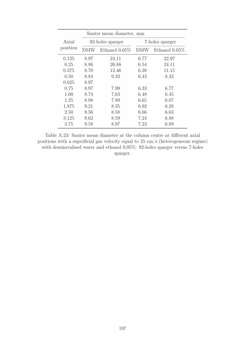
Sauter mean diameter, mm
Axialposition
92-holes sparger 7-holes sparger
DMW Ethanol 0.05% DMW Ethanol 0.05%
0.125 8.97 24.11 6.77 22.970.25 8.86 26.88 6.54 24.110.375 8.70 12.46 6.38 11.150.50 8.84 9.33 6.43 8.330.625 8.970.75 8.97 7.99 6.33 6.771.00 8.74 7.63 6.48 6.451.25 8.98 7.89 6.65 6.071.875 9.21 8.35 6.92 6.282.50 9.56 8.58 6.66 6.633.125 9.62 8.59 7.24 6.883.75 9.58 8.97 7.23 6.89
Table A.23: Sauter mean diameter at the column centre at different axialpositions with a superficial gas velocity equal to 25 cm/s (heterogeneous regime)
with demineralised water and ethanol 0.05%: 92-holes sparger versus 7-holessparger.
197

Sauter mean diameter, mm
Radialposition
92-holes sparger 7-holes sparger
H/D=2.50 H/D=0.25 H/D=2.50 H/D=0.25
0.00 7.25 8.30 6.81 8.300.20 6.80 8.12 6.96 8.120.40 7.18 7.74 6.79 7.740.60 7.13 7.05 6.40 7.050.80 7.02 7.37 6.23 7.37
Table A.24: Sauter mean diameter with a superficial gas velocity equal to 3 cm/s(homogeneous regime) with demineralised water at two different heights(H/D=2.5 versus H/D=0.25): 92-holes sparger versus 7-holes sparger.
Sauter mean diameter, mm
Radialposition
92-holes sparger 7-holes sparger
H/D=2.50 H/D=0.25 H/D=2.50 H/D=0.25
0.00 9.05 8.00 8.40 8.000.20 8.84 8.05 8.20 8.050.40 8.63 8.01 7.84 8.010.60 7.51 7.90 7.07 7.900.80 6.34 7.48 6.60 7.48
Table A.25: Sauter mean diameter with a superficial gas velocity equal to 16cm/s (heterogeneous regime) with demineralised water at two different heights
(H/D=2.5 versus H/D=0.25): 92-holes sparger versus 7-holes sparger.
198

Appendix B
Drag laws
B.1 Drag laws for spherical bubbles
The first drag law was formulated by Stokes (1851), for Reb << 1 and sphericaltotally contaminated bubbles:
CD =24
Reb. (B.1)
Schiller & Naumann (1935) corrected this relation to extend the field until Reb ≤800, and it is the most utilized for bubble columns in homogeneous regime:
CD =24
Reb
(1 + 0.15Re0.687b
). (B.2)
A constant value for Reb > 1000 is considered in order to use this correlation in alarger field:
CD =
{24Reb
(1 + 0.15Re0.687b ) Reb ≤ 1000;
0.44 Reb ≥ 1000.(B.3)
Subsequently, different correlations have been developed; in general the coefficientdepends on the Reynolds number.
Other important drag laws were proposed by Zhang & Vanderheyden (2002):
CD = 0.44 +24
Reb+
1
1 +√Reb
(B.4)
and by Fdhila & Duineveld (1996):
CD =24
Reb
(1 + 0.9135Re0.6305b
). (B.5)
B.2 Drag laws model for oblate bubbles
For a deformed bubble, the drag coefficient depends on the Reynolds, the Eötvösand the Morton number:
CD = f(Reb, Eo, Mo). (B.6)
In certain cases, some authors use the Weber number or the Frounde number. Boththese numbers can be written in function of the Reynolds, Eötvös and Morton
199

number. It is necessary to take three independent dimensionless numbers.
We =ρq u
2r deqσ
= Re2b
(Mo
Eo
)1/2
; (B.7)
Fr =
√ρq v2r
Δρ g deq=
√We
Eo(B.8)
where ur is the relative velocity between the two phases.For different operating conditions, Fan et al. (1999) found an empirical correl-
ation to obtain directly the relative velocity. It can give a first idea for severalsystems, with spherical and ellipsoidal bubbles:
ur =
(σg
ρq
)1/4[(
Mo−1/4
Kb
(Δρ
ρq
)5/4
d′2)−n
+
(2 c
d′+
Δρd′
2 ρq
)−n/2]−1/n
(B.9)
with:
d′ = db
√ρl g
σ;
Kb = max(Kb0 Mo−0.038, 12
);
Kb0 = 10.2 for organic and 14.7 for aqueous solution;n = 1.6 for clean and 0.8 for contaminated systems;c = 1.2 for pure liquid and 1.4 for multi-composition liquid.
Maxworthy et al. (1996) proposed to use for deformed bubbles:
CD =
⎧⎪⎪⎨⎪⎪⎩min
{43
Eo
Wec,8
3Eo2/3
}for Eo ≤ 7.12
8
3
4Eo
(9.5 + Eo)for Eo ≥ 7.12
(B.10)
where:Wec = max(0.517ln(Mo) + 7.624, 2.326) (B.11)
Tomiyama (1998) suggested to use for deformed bubbles:
CD =8
3
Eo
(4 + Eo). (B.12)
This expression for Eo > 40 tends to a constant value of 8/3, as calculated byDavies & Taylor (1950) for a regime of spherical cap.
In case of spherical bubbles Tomiyama (1998) used the drag law of Levich(1962), available for Re >> 1:
CD =48
Reb. (B.13)
Tomiyama (1998) obtained a correlation usable for every regime:
CD = max
{min
{24
Reb
(1 + 0.15Re0.687b
),48
Reb
},8
3
Eo
(4 + Eo)
}. (B.14)
200

Dijkhuizen et al. (2010) proposed a correlation suitable for spherical and deformedbubbles:
CD =
√CD
2 (Reb) + CD2 (Eo); (B.15)
CD (Reb) =16
Reb
(1 +
Reb
8 + 0.5(Re+ 3.315Reb
0.5)) ; (B.16)
CD (Eo) =4Eo
(9.5 + Eo). (B.17)
Zhang et al. (2006) suggested a shorter correlation that gives results very similarto the others:
CD =2
3
√Eo. (B.18)
In case of boiling regime, the most used correlation was proposed by Ishii & Zuber(1979), considering the effect of the gas fraction inside:
CD =8
3(1− αg)
2. (B.19)
Tomiyama et al. (2002) coined also another correlation:
CD =8
3
Eo
E2/3(1− E2
)−1Eo+ 16E4/3
F−2 (B.20)
where:
F =sin−1
(√1− E2
)− E(√
1− E2)
(1− E2)(B.21)
and E is the shape factor that is:
E =1
1 + 0.163Eo0.757. (B.22)
Hosokawa & Tomiyama (2009) calculated E starting by the E0, the shape factorin an infinite medium.
E0 =
⎧⎪⎪⎪⎪⎨⎪⎪⎪⎪⎩1 Ta ≥ 1;
{0.81 + 0.206 tanh [(0.8− log10 Ta) 2]}3 39.8 ≥ Ta;
0 39.8 ≥ Ta.
(B.23)
Using the Tadaki number:Ta = Reb Mo0.23. (B.24)
Starting by E0, it is possible to obtain E:
E = E0 max{1− 0.35
y
D, 0.65
}(B.25)
where y is the distance by the wall and D the diameter of the column.
201
BibliographyDavies, R. M. & Taylor, G. (1950), ‘The mechanics of large bubbles rising through
extended liquids and through liquids in tubes.’, Proceedings A - The Royal So-ciety 200, 1062.
Dijkhuizen, W., Roghair, I., Annaland, M. & Kuipers, J. (2010), ‘DNS of gasbubbles behaviour using an improved 3D front tracking model-drag force on isol-ated bubbles and comparison with experiments.’, Chemical Engineering Science65(4), 1415–1426.
Fan, L., Yang, G., Lee, D. & Luo, X. (1999), ‘Some aspects of high-pressure phe-nomena of bubbles in liquids and liquid-solid suspensions.’, Chemical EngineeringScience 54, 4681–4709.
Fdhila, R. & Duineveld, P. (1996), ‘The effect of surfactant on the rise of sphericalbubble at high reynolds and peclet number.’, Physics of Fluid 8(2), 310–321.
Hosokawa, S. & Tomiyama, A. (2009), ‘Multi-fluid simulation of turbulent bubblyin pipe flows.’, International Journal of Multiphase flow 28, 1497–1519.
Ishii, M. & Zuber, N. (1979), ‘Drag coefficient and relative velocity in bubbly,droplet or particulate flows’, American Institute of Chemical Engineering Journal25(5), 843–855.
Levich, V. G. (1962), Physicochemical Hydrodynamics, Prentice Hall, EnglewoodCliffs, NJ.
Maxworthy, T., Gnann, C., Kürten, M. & Durst, F. (1996), ‘Experiments on therise of air bubbles in clean viscous liquids.’, Journal of Fluid Mechanics 321, 421–441.
Schiller, L. & Naumann, N. (1935), ‘A drag coefficient correlation.’, Vdi Zeitung77, 318.
Stokes, G. G. (1851), ‘On the effect of the internal friction of fluids on the motionof pendulums.’, Cambridge Philos. Trans. 9, 8–106.
Tomiyama, A. (1998), ‘Struggle with computational bubble dynamics.’, MultiphaseScience and Technology 10(4), 369.
Tomiyama, A., Celata, G., Hokosawa, S. & Yoshida, S. (2002), ‘Terminal velocity ofsingle bubbles in surface tension force dominant regime.’, International Journalof Multiphase flow 28, 1497–1519.
Zhang, D., Deen, N. G. & Kuipers, J. A. M. (2006), ‘Numerical simulation ofdynamic flow behavior in a bubble column: A study of closures for turbulenceand interface forces’, Chemical Engineering Science 61, 7593–7608.
Zhang, D. & Vanderheyden, W. (2002), ‘The effects of mesoscale structures on thedisperse two-phase flows and their closures for dilute suspensions.’, InternationalJournal of Multiphase Flow 28, 805–822.
202

Appendix C
Favre-like average
C.1 Favre-like average definitionThe Favre-like or phase average, in two-fluid models, allows to make a time averageof the property of a phase by taking into account the instantaneous local volumefraction of this phase (Favre 1965, O’Brien 2012). The Favre mean can replace theReynolds mean in multiphase flows (Burns et al. 2004).
A generic variable Θ, can be divided into a mean part Θ and a fluctuating partΘ′′ if a phase-fraction weighted average is used (O’Brien 2014):
Θ = Θ + Θ′′, (C.1)
Θ =
∫αi(t)Θ(t)dt∫αi(t)dt
, (C.2)
that is equal to:
Θ =αiΘ
αi
, (C.3)
where αi is the instantaneous local gas volume fraction of the phase i.In this work different properties are calculated with both Reynolds and Favre-
like average: axial velocities of the two phases, Sauter mean diameter and turbu-lence properties.
The gas volume fraction (and consequently the liquid volume fraction) is thesame by using Reynolds and Favre-like averages.
The axial gas velocity with the Favre-like average seen by the bubbles (ug) iscalculated as follows:
ug =αgug
αg
, (C.4)
where ug is the instantaneous axial gas velocity and αg is the instantaneous gasvolume fraction.
Consequently, by using the Reynolds average, the axial gas velocity can bedivided into a mean part αg and a fluctuating part u′
g, as follows (O’Brien 2014):
αg = αg + α′g, (C.5)
while, by using the Favre-like average, the axial gas velocity can be divided into amean part αg and a fluctuating part u′
g (O’Brien 2014):
αg = αg + α′′g . (C.6)
203

Concerning the axial liquid velocity, the Favre-like average seen by the liquid phaseshould be considered (ul):
ul =αlul
αl
, (C.7)
where ul is the instantaneous axial liquid velocity and αl is the instantaneousliquid volume fraction, that is the complementary of the instantaneous gas volumefraction.
The Sauter mean diameter with the Favre-like average seen by the bubbles(d32,g) is defined as:
d32,g =αgd32αg
, (C.8)
where d32 is the instantaneous Sauter mean diameter.The turbulence properties refer to the liquid, but they can affect bubble co-
alescence and breakage phenomena. For this reason, the Favre-like averages seenby both the bubbles and the liquid are calculated. Concerning the turbulence kin-etic energy, the Favre-like averages seen by the bubbles kg and the liquid kl arecalculated respectively as:
kg =αgk
αg
(C.9)
and
kl =αlk
αl
, (C.10)
where k is the instantaneous turbulence kinetic energy.The Favre-like averages of the turbulence dissipation rate seen by the bubbles
εg and liquid εl
εg =αgε
αg
(C.11)
andεl =
αlε
αl
, (C.12)
where ε is the instantaneous turbulence dissipation rate.
C.2 Favre-like average effects
The effect of the Favre-like average on the properties listed above is studied in thiswork by comparing the Reynolds averages with the Favre-like averages. In this partof the work, the radial profiles, obtained with the column φ 0.4 m and a superficialgas velocity equal to 0.16 m/s (heterogeneous regime) at H/D=2.5, are compared.
The effect of the Favre-like average on the axial liquid velocities is quite small(Fig. C.1). The Favre-like average seen by the liquid is slightly smaller than theReynold average for every radial position, except at the wall, where the means areidentical.
The effect on the axial gas velocity could be considered. Expect at the wall, theuse of the Favre-like average, instead of the Reynolds average, causes an increaseof this property, as shown in Fig. C.2.
204

-1
-0.5
0
0.5
1
0 0.25 0.5 0.75 1
Axi
al li
quid
vel
ocity
, m/s
Radial position
Figure C.1: Radial profile of the axial liquid velocity for a superficial gas velocityof 0.16 m/s at H/D=2.5. Experimental data (�) versus CFD results obtained byconsidering the Reynolds average (solid line) and the Favre-like average seen by
the liquid (dotted line).
-0.5
0
0.5
1
1.5
0 0.25 0.5 0.75 1
Axi
al b
ubbl
e ve
loci
ty, m
/s
Radial position
Figure C.2: Radial profile of the axial gas velocity for a superficial gas velocity of0.16 m/s at H/D=2.5. Experimental data (�) versus CFD results obtained by
considering the Reynolds average (solid line) and the Favre-like average seen bythe bubbles (dashed line).
205

The Sauter mean diameter, if calculated with the Favre-like average seen by thebubbles, has an increase lower than 10% . The radial profile shape is the same andthe discrepancies are lower close to wall. The radial profiles of the Sauter meandiameter are reported in Fig. C.3.
0
2
4
6
8
10
12
0 0.25 0.5 0.75 1
Saut
er m
ean
diam
eter
, mm
Radial position
Figure C.3: Radial profile of the Sauter mean diameter for a superficial gasvelocity of 0.16 m/s at H/D=2.5. Experimental data (�) versus CFD resultsobtained by considering the Reynolds average (solid line) and the Favre-like
average seen by the bubbles (dashed line).
The effects of the Favre-like averages on the turbulence properties are almostnegligible, as shown in Fig. C.4 and C.5 for turbulence kinetic energy and tur-bulence dissipation rate respectively. The radial profile calculated with Favre-likeaverage seen by the bubbles is slightly higher than the classical one, while thosecalculated with the Favre-like average seen by the liquid is slightly lower.
For every property, the radial profile is slightly influenced by the Favre-likeaverage and its effect is often negligible. The Favre-like average seen by the bubblesslightly increases every property, while the Favre-like average seen by the liquid hasthe opposite effect.
206

0
0.05
0.1
0.15
0.2
0.25
0.3
0.35
0.4
0 0.25 0.5 0.75 1
Turb
ulen
ce k
inet
ic e
nerg
y, m
2 /s2
Radial position
Figure C.4: Radial profile of the turbulence kinetic energy for a superficial gasvelocity of 0.16 m/s at H/D=2.5. Experimental data (�) versus CFD resultsobtained by considering the Reynolds average (solid line) and the Favre-like
average seen by the bubbles (dashed line) and the liquid (dotted line).
0
0.2
0.4
0.6
0.8
1
1.2
1.4
1.6
0 0.25 0.5 0.75 1
Turb
ulen
ce d
issip
atio
n ra
te, m
2 /s3
Radial position
Figure C.5: Radial profile of the turbulence dissipation rate for a superficial gasvelocity of 0.16 m/s at H/D=2.5. Experimental data (�) versus CFD resultsobtained by considering the Reynolds average (solid line) and the Favre-like
average seen by the bubbles (dashed line) and the liquid (dotted line).
207

BibliographyBurns, A. D. B., Frank, T., Hamill, I. & Shi, J. M. (2004), The Favre averaged
drag model for turbulent dispersion in eulerian multi-phase flows., in ‘5th Inter-national Conference on Multiphase Flow, ICMF-2004’, Yokohama, Japan.
Favre, A. (1965), ‘Equations des gaz turbulents compressibles. i. Formes générales.’,Journal de Mécanique 4, 361–390.
O’Brien, T. (2012), A Favre-averaged turbulence model for gas-particle flows., in‘2012 AIChE Annual Meeting’, Pittsburgh, Pennsylvania, USA.
O’Brien, T. (2014), A multiphase turbulence theory for gas-solids flows using Favre-averaging., in ‘2014 NETL Workshop on Multiphase Flow Science’, Morgantown,West Virginia, USA.
208