MODELLING OF NONLINEAR LONG MEMORY - mii.lt · MODELLING OF NONLINEAR LONG MEMORY Doctoral...
125
VILNIUS UNIVERSITY IEVA GRUBLYTĖ MODELLING OF NONLINEAR LONG MEMORY Doctoral Dissertation Physical Sciences, Mathematics (01P) Vilnius, 2017
Transcript of MODELLING OF NONLINEAR LONG MEMORY - mii.lt · MODELLING OF NONLINEAR LONG MEMORY Doctoral...
VILNIUS UNIVERSITY
IEVA GRUBLYTĖ
MODELLING OF NONLINEAR LONG MEMORY
Doctoral DissertationPhysical Sciences, Mathematics (01P)
Vilnius, 2017

The scientific work was carried out in 2013-2017 at Vilnius University and Universityof Cergy-Pontoise (France).
Scientific Supervisor - Prof. Dr. Habil. Donatas Surgailis (Vilnius University,Physical sciences, Mathematics - 01P).Scientific Advisor - Prof. Dr. Paul Doukhan (University of Cergy-Pontoise, Phys-ical sciences, Mathematics - 01P).
VILNIAUS UNIVERSITETAS
IEVA GRUBLYTĖ
NETIESINIAI ILGOS ATMINTIES MODELIAI
Daktaro disertacijaFiziniai mokslai, matematika (01P)
Vilnius, 2017
Disertacija rengta 2013-2017 metais Vilniaus Universitete ir Cergy-Pontoise Univer-sitete (Prancūzija).
Mokslinis vadovas - prof. habil. dr. Donatas Surgailis (Vilniaus universitetas,fiziniai mokslai, matematika - 01P).Mokslinis konsultantas - prof. dr. Paul Doukhan (Cergy-Pontoise universitetas,fiziniai mokslai, matematika - 01P).

Contents
Notations and Abbreviations 7
1 Introduction 9
2 State of the art 152.1 Long memory . . . . . . . . . . . . . . . . . . . . . . . . . . . . . . . 152.2 Long memory processes . . . . . . . . . . . . . . . . . . . . . . . . . . 182.3 Estimation . . . . . . . . . . . . . . . . . . . . . . . . . . . . . . . . . 23
3 Projective stochastic equations and nonlinear long memory 263.1 Introduction . . . . . . . . . . . . . . . . . . . . . . . . . . . . . . . . 263.2 Projective processes and their properties . . . . . . . . . . . . . . . . 283.3 Projective stochastic equations . . . . . . . . . . . . . . . . . . . . . . 313.4 Examples . . . . . . . . . . . . . . . . . . . . . . . . . . . . . . . . . 363.5 Simulations . . . . . . . . . . . . . . . . . . . . . . . . . . . . . . . . 403.6 Modifications . . . . . . . . . . . . . . . . . . . . . . . . . . . . . . . 423.7 Long memory . . . . . . . . . . . . . . . . . . . . . . . . . . . . . . . 45
4 A nonlinear model for long memory conditional heteroscedasticity 524.1 Introduction . . . . . . . . . . . . . . . . . . . . . . . . . . . . . . . . 534.2 Stationary solution . . . . . . . . . . . . . . . . . . . . . . . . . . . . 554.3 Weak dependence . . . . . . . . . . . . . . . . . . . . . . . . . . . . . 66
Projective weak dependence coefficients . . . . . . . . . . . . . . . . . 67τ -weak dependence coefficients . . . . . . . . . . . . . . . . . . . . . . 69
4.4 Strong dependence . . . . . . . . . . . . . . . . . . . . . . . . . . . . 704.5 Leverage . . . . . . . . . . . . . . . . . . . . . . . . . . . . . . . . . . 774.6 A generalized nonlinear model for long memory conditional heteroscedas-
ticity . . . . . . . . . . . . . . . . . . . . . . . . . . . . . . . . . . . . 80Stationary solution . . . . . . . . . . . . . . . . . . . . . . . . . . . . 80
5
Model properties . . . . . . . . . . . . . . . . . . . . . . . . . . . . . 884.7 A simulation study . . . . . . . . . . . . . . . . . . . . . . . . . . . . 89
5 Quasi-MLE for quadratic ARCH model with long memory 935.1 Introduction . . . . . . . . . . . . . . . . . . . . . . . . . . . . . . . . 935.2 QML estimators . . . . . . . . . . . . . . . . . . . . . . . . . . . . . . 955.3 Main results . . . . . . . . . . . . . . . . . . . . . . . . . . . . . . . . 985.4 Lemmas . . . . . . . . . . . . . . . . . . . . . . . . . . . . . . . . . . 1025.5 Simulation study . . . . . . . . . . . . . . . . . . . . . . . . . . . . . 110
Conclusions 113
A Lemmas 114
B Nested Volterra series 117
6

Notations and Abbreviations
N - the set of natural numbers, N = 1, 2, . . .
Z - the set of natural numbers, Z = . . . ,−2,−1, 0, 1, 2, . . .
R - the set of real numbers
C,C(. . . ) denote generic constants, possibly dependent on the variables intobrackets, which may be different at different locations
EX denotes the mean of random variable X
Var(X) denotes the variance of random variable X
Cov(X, Y ) denotes the covariance of random variables X, Y
sign(·) is a sign function
1(·), 1(.) denote the indicator function
x ∧ y denotes min(x, y) for real numbers x, y
x ∨ y denotes max(x, y) for real numbers x, y
L is a lag operator, i.e. LXt = Xt−1
B(·, ·) is a beta function
Γ(·) is a gamma function
BH(t) denotes fractional Brownian motion where H is the Hurst parameter
→D[0,1] denotes the weak convergence of random processes in the Skorohodspace D[0, 1]
7

‖ · ‖p := E1/p| · |p, p ≥ 1 denotes Lp norm
`∞(R) denotes the space of all bounded functions on R
i.i.d independent identically distributed
r.v random variable
a.s. almost surely
r.h.s right hand side
l.h.s left hand side
w.r.t with respect to
8
Chapter 1
Introduction
Long memory as an object of research
A discrete-time second-order stationary process Xt, t ∈ Z is called long memory ifits covariance γ(k) = Cov(X0, Xk) decays slowly with the lag in such a way that itsabsolute series diverges:
∞∑k=1|γ(k)| =∞. (1.1)
In the converse case when∞∑k=1|γ(k)| <∞ and
∞∑k=1
γ(k) 6= 0 (1.2)
the process Xt is said to have short memory. Negative memory is defined as
∞∑k=1|γ(k)| <∞ and
∞∑k=1
γ(k) = 0. (1.3)
Long memory processes have different properties from short memory (in particular,i.i.d.) processes. Long memory processes have been found to arise in a variety ofphysical and social sciences. See, e.g., the monographs Beran (1997), Doukhan et al.(2003), Giraitis et al. (2012), Beran et al. (2013) and the references therein.
Conditions (1.1)-(1.3) defining long, short and negative memory are very general.A useful asymptotic theory and statistical inference is possible if one specifies therate of decay of γ(k) at infinity. Particularly, (1.1) is often specified as
γ(k) = |k|−1+2dLγ(|k|), |k| ≥ 1, 0 < d < 1/2 (1.4)
9
orγ(k) ∼ cγ|k|−1+2d, k →∞, 0 < d < 1/2, cγ > 0, (1.5)
where Lγ : [1,∞)→ R is a slowly varying function at infinity. Parameter d ∈ (0, 1/2)in (1.4) and (1.5) is called the long memory parameter of Xt. It characterizes theintensity of long memory of the process Xt: when d > 0 is small the covariancefunction decays relatively fast and the intensity of long memory is small, while inthe case when d is close to 1/2 the covariance function decays very slowly since theexponent −1+2d is almost zero, and the corresponding process Xt has very strongmemory.
Probably, the most important model of long memory processes is the linear, ormoving average process
Xt =∑s≤t
bt−sζs, t ∈ Z, (1.6)
where ζs, s ∈ Z is a standardized i.i.d. sequence, and the moving average co-efficients bj decay slowly so that ∑∞j=0 |bj| = ∞, ∑∞j=0 b
2j < ∞. The last con-
dition guarantees that the series in (1.6) converges in mean square and satisfiesEXt = 0, EX2
t = ∑∞j=0 b
2j < ∞. In the literature it is often assumed that the
coefficients regularly decay as
bj ∼ κjd−1, j →∞ (∃ κ > 0, 0 < d < 1/2). (1.7)
Condition (1.7) guarantees (1.5), i.e. that
γ(k) =∞∑j=0
bjbk+j ∼ κ2B(d, 1− 2d)k−1+2d, k →∞ (1.8)
and hence ∑∞k=1 |γ(k)| = ∞. Thus, the parameter d in (1.7) is the long memoryparameter of Xt as defined in (1.5).
An important property of the linear process in (1.6)-(1.7) is the fact that its(normalized) partial sums process Sn(τ) := ∑[nt]
j=1Xj, τ ≥ 0 tends to a fractionalBrownian motion (Davydov (1970)), viz.,
n−d−1/2Sn(τ) →D[0,1] σ(d)BH(t), (1.9)
where H = d + 12 is the Hurst parameter, σ(d)2 := κ2B(d, 1 − 2d)/d(1 + 2d) > 0
and→D[0,1] denotes the weak convergence of random processes in the Skorohod spaceD[0, 1]. By definition, fractional Brownian motion is a Gaussian process with zero
10
mean and covariance function
EBH(s)BH(t) = 12(t2H + s2H − |t− s|2H), t, s ≥ 0. (1.10)
Note that the normalization in (1.9) grows faster than the classical normalizationn1/2 in Donsker’s invariance principle for weakly dependent summands, and the limitprocess BH has dependent increments in contrast to the usual Brownian motion withindependent increments. Fractional Brownian motion is H-self-similar and plays avery important role in many applications of stochastic processes. The above men-tioned properties of the partial sums limit are characteristic to long memory althoughin general the covariance decay as in (1.5) does not imply a fractional Brownian mo-tion limit of the partial sums process.
Motivation and aims of the thesis
It is well-known that the linear model (1.6) has its drawbacks and sometimes is notcapable of incorporating empirical features (“stylized facts”) of some observed timeseries. The “stylized facts” may include typical asymmetries, clusterings, and othernonlinearities which are often observed in financial data, together with long memory.A very important stylized fact of asset returns is conditional heteroscedasticity, orthe property of the conditional variance
Var[Xt+1|Ft] = E[(Xt+1 − E[Xt+1|Ft])2|Ft]
being a random process and not a constant like in linear models. Here, Ft isthe “historic” σ-field containing “all available information” and E[Xt+1|Ft] is thebest forecast of Xt+1 given the “information” Ft. For the linear process in (1.6)and Ft = σζs, s ≤ t, the best forecast is E[Xt+1|Ft] = b1ζt + b2ζt−2 + . . . andXt+1 − E[Xt+1|Ft] = b0ζt+1 is independent of Ft so that the conditional varianceis constant: Var[Xt+1|Ft] = b2
0Eζ2t , meaning that this model is conditionally ho-
moscedastic. Therefore developing nonlinear models with long memory presents con-siderable interest.
Problems and main results
The principal goal of this thesis is to introduce new nonlinear models with long mem-ory that could be used for modelling of financial returns and statistical inference.
1. Projective stochastic equations (Chapter 3).
11
The main goal is to introduce a new class of nonlinear processes which generalizethe linear model in (1.6)-(1.7) and enjoy similar long memory properties to (1.8)and (1.9). For this, we define projective moving averages Xt, t ∈ Z, where Xt
is a Bernoulli shift written as a backward martingale transform of the innovationsequence. We introduce a new class of nonlinear stochastic equations for projectivemoving averages, termed projective equations, involving a (nonlinear) kernel Q and alinear combination of projections ofXt on “intermediate” lagged innovation subspaceswith given coefficients αi, βi,j. We obtain conditions for solvability of these equations.We also show that under certain conditions on kernel and coefficients, the solutionexhibits covariance and distributional long memory, with fractional Brownian motionas the limit of the corresponding partial sums process. Results are presented inChapter 3 and Grublytė and Surgailis (2014).
2. A nonlinear model for long memory conditional heteroscedasticity (Chapter 4).The main goal is to introduce a new class of conditionally heteroscedastic processes
that generalize some of the already known models and are able to model long memoryand other stylized facts in certain cases. For this, we discuss a class of conditionallyheteroscedastic time series models satisfying the ARCH-type equation rt = ζtσt,where ζt is a noise sequence and the conditional standard deviation σt is a nonlinearfunction Q depending on a linear combination of past values rs, s < t with coefficientsbj. We obtain the conditions for the existence of stationary solution rt with finitep-th moment, 0 < p < ∞. Weak dependence properties of rt are studied, includingthe invariance principle for partial sums of Lipschitz functions of rt. The case whenQ is the square root of a quadratic polynomial corresponds to a quadratic ARCH(QARCH) model and is of special interest. We prove that in this case rt can exhibita leverage effect and long memory, in the sense that the squared process r2
t haslong memory autocorrelation and its normalized partial sums process converges toa fractional Brownian motion. Analogous results are obtained for the generalizedversion of the model described above where the conditional variance satisfies an AR(1)equation, i.e. the volatily form includes the lagged volatilities from the past. We alsoobtain a new condition for the existence of higher moments of rt which does notinclude the Rosenthal constant. A short simulation study showing the behavior ofprocesses defined by this model is included. Results are presented in Chapter 4 andDoukhan et al. (2016), Grublytė and Škarnulis (2017).
3. Quasi-MLE for quadratic ARCH model with long memory (Chapter 5).The goal is to provide the asymptotic results for quasi-maximum likelihood esti-
mators in parametric version of long memory QARCH model introduced in Chapter4 (also Doukhan et al. (2016), Grublytė and Škarnulis (2017)). Similarly as in Beran
12
and Schützner (2009) we discuss several QML estimators: the estimator involvingexact conditional variance depending on infinite past and its more realistic versionwhere the volatilities depend only on finite number of returns from past. Undercertain moment conditions we prove consistency and asymptotic normality of thecorresponding QML estimators, including the estimator of long memory parameter0 < d < 1/2. Results are presented in Chapter 5 and Grublytė et al. (2017).
The novelty
New nonlinear models with long memory for modelling of financial returns are de-veloped in this thesis. These processes are defined as stationary solutions of certainnonlinear stochastic difference equations involving a given i.i.d. “noise”. Solvabil-ity of these equations is studied and covariance and distributional long memory isproved. Finally, for a particularly tractable nonlinear parametric model with longmemory (GQARCH) consistency and asymptotic normality of quasi-ML estimatorsare proved.
The processes studied in the thesis are new and have not been investigated in ascientific literature before.
Methods
Many proofs in the thesis use the idea of projections (discussed in more detail inChapter 3, Section 3.2). Besides that, other standard tools from probability theory,functional analysis, mathematical statistics and time series analysis were used.
Dissemination
The results were presented in the following conferences and seminars:
• 54th conference of Lithuanian Mathematical Society, Vilnius (Lithuania), June19-20, 2013.
• 55th conference of Lithuanian Mathematical Society, Vilnius (Lithuania), June26-27, 2014.
• 11th International Vilnius Conference on Probability Theory and MathematicalStatistics, Vilnius (Lithuania), June 30 - July 4, 2014.
• Séminaire SAMM: Statistique, Analyse et Modélisation Multidisciplinaire, Uni-versité Paris 1 Panthéon-Sorbonne, Paris (France), November 28, 2015.
13
• 8th annual SoFiE (The Society for Financial Econmetrics) conference, Aarhus(Denmark), June 23 - 26, 2015.
• Conference “Stochastic Processes”, Luminy (France), February 15-19, 2016.
• Seminar at “Workshop on Dependence”, Institut Henri Poincaré, Paris (France),September 27, 2016.
Publications
• I. Grublytė, D. Surgailis (2014). Projective stochastic equations and nonlinearlong memory, Adv. in Appl. Probab., 46(4):1-22.
• P. Doukhan, I. Grublytė, D. Surgailis (2016). A nonlinear model for long mem-ory conditional heteroscedasticity, Lith. Math. J. 56(2):164–188.
• I. Grublytė, A. Škarnulis (2017). A generalized nonlinear model for long mem-ory conditional heteroscedasticity, Statistics 51(1):123-140.
• I. Grublytė, D. Surgailis, A. Škarnulis (2017). QMLE for quadratic ARCHmodel with long memory. J. Time Ser. Anal. 38(4):535–551.
Structure of thesis
The thesis consists of Introduction, State of the Art, three Chapters, Conclusions,two Appendixes and Bibliography. The review of aims and problems is given inIntroduction. State of the Art presents an overview of the scientific work in thisfield. Chapter 3 introduces nonlinear processes defined through projective stochasticequations. Chapter 4 presents a very general class of nonlinear conditionally het-eroscedastic models. A separate case of (G)QARCH model ((Generalized) QuadraticARCH) is studied in more detail. Chapter 5 considers the estimation of parametersin generalized QARCH models using QML method. The results of the thesis aresummarized in Conclusions.
Acknowledgements
I’m very grateful to my advisors prof. Donatas Surgailis and prof. Paul Doukhan fortheir guidance during my PhD thesis.
14

Chapter 2
State of the art
In this chapter, firstly we present some of the most commonly used definitions oflong memory. Next, we briefly review the (nonlinear) long memory processes studiedin the literature. Finally, a short overview on the estimation of parameters in thesemodels is presented at the end of the chapter.
2.1 Long memory
Long memory processes were studied in a literature by numerous authors, see, e.g.,the monographs Beran (1997), Doukhan et al. (2003), Giraitis et al. (2012) and thereferences therein. The problems considered include the detection of long memory,estimation of long memory parameter, limit theorems for long memory processes,simulation of processes, etc. According to Samorodnitsky (2007), the first attemptsto study long memory start with the papers of Mandelbrot and his coleagues in 1960s(see Mandelbrot (1965), Mandelbrot and Van Ness (1968)) where the authors seekto explain the phenomenon observed by Hurst (1951) in the empirical data of Nileflows.
Hurst (1951) considered the R/S statistic for Nile river data defined as follows.Given a sequence of n observations X1, X2, . . . , Xn, define the partial sum sequenceSm = X1 + · · · + Xm for m = 0, 1, . . . (with S0 = 0). The R/S statistic (range ofobservations/sample standard deviation) takes the following form
R
S(X1, . . . , Xn) =
max0≤i≤n(Sn − inSn)−min0≤i≤n(Sn − i
nSn)
( 1n
∑ni=1(Xi − 1
nSn)2)1/2 .
It is known that if X1, X2, . . . is a stationary ergodic sequence of random variableswith a common mean µ and finite variance, such that the standard central limit
15
theorem holds, then growth rate of R/S statistic is the square root of the samplesize. However, Hurst noticed that the growth rate in R/S statistic for the Nile flowsdata was closer to n0.74. This phenomenon was called Hurst phenomenon and led tovarious efforts to explain it.
The fact that the R/S growth rate has unusual behavior suggested that some of theassumptions are not satisfied in the previous example. Mandelbrot (1965) decidedto refuse the assumption of the validity of the central limit theorem for processXt and proposed to consider a finite variance model with very slowly decayingcorrelations. This approach appeared to be very succesfull. Fractional GaussianNoise (the difference of fractional Brownian motion BH , H > 0) defined as
Xt := BH(t)−BH(t− 1),
with autocovariances Cov(Xt+n, Xt) = 2(|n+1|2H + |n−1|2H−2n2H
)is the simplest
example of such model and gives the growth rate nH in the R/S statistic.Since then, various other definitions of the long memory were proposed (see eg.
Samorodnitsky (2007), where the most popular definitions are summarized). Mostoften (due to simplicity and easy estimation from data) the definitions use the secondorder properties of stochastic processes, for example, asymptotics of covariances,spectral density, variance of partial sums.
The following definition of long memory is based on the slow decay of covariances.
Definition 2.1.1 A covariance stationary process X(t), t ∈ Z is said to have longmemory if its autocovariances γ(k) = Cov(Xt, Xt−k) are not absolutely summable,i.e. ∑
k∈Z|γ(k)| =∞. (2.1)
The process is said to have short memory if
∞∑k=1|γ(k)| <∞ and
∞∑k=1
γ(k) 6= 0. (2.2)
The process is said to have negative memory if
∞∑k=1|γ(k)| <∞ and
∞∑k=1
γ(k) = 0. (2.3)
The definition above imposes very general conditions for autocovariances. It isoften useful to go a bit further and specify the decay rate of covariances. Let us firstintroduce the notion of slowly varying functions.
16
Definition 2.1.2 A function L is said to be slowly varying at infinity, if L is positiveon [a;∞), for some a > 0, and ∀t > 0:
limx→∞
L(tx)L(x) = 1.
Definition 2.1.3 A stationary process X(t), t ∈ Z is said to have long memory, ifthe autocovariance function γ(k) = Cov(Xt, Xt−k) decays hyperbolically, as k →∞,
γ(k) = k2d−1L(k), 0 < d < 1/2 (2.4)
where L(·) is a slowly varying function at infinity. The parameter d is called a long-memory parameter.
Clearly, if the process X(t), t ∈ Z satisfies (2.4), it also satisfies (2.1), theconverse not necessarily being truth.
Another common definition of long memory considers the limiting distributionof normalized partial sums process Sn(τ) := ∑[nτ ]
j=1Xj, τ ≥ 0 where [x] denotes theinteger part of x. Let us first give some definitions (see eg. Giraitis et al. (2016)).
Definition 2.1.4 (i) A real valued stochastic process Z(t), t ∈ R with Z(0) = 0 issaid to have stationary increments if for any integer k > 0, and for any t1 < t2 <
· · · < tk, ti ∈ R, i = 1, . . . , k and h ∈ R, the joint distributions of Z(tj + h) −Z(h), 1 ≤ j ≤ k and Z(tj)− Z(0), 1 ≤ j ≤ k are the same. In other words, if forany h ∈ R,
Z(h+ t)− Z(h), t ∈ R =fdd Z(t)− Z(0), t ∈ R.
(ii) A process Z(t), t ∈ R is said to be self-similar with index H > 0, if finitedimensional distributions of Z(at) and aHZ(t) are the same for all a > 0:
Z(at), t ∈ R =fdd aHZ(t), t ∈ T.
In other words, for any a > 0, k = 1, 2, . . . , and for any tj ∈ R, 1 ≤ j ≤ k,
(Z(at1), . . . , Z(atk)) =fdd aH(Z(t1), . . . , Z(tk)).
The process is said to be H-sssi if it is self-similar and has stationary increments. Afractional Brownian motion BH is an example of a Gaussian H-sssi process and playsa very important role in many applications of stochastic processes.
17
Definition 2.1.5 Let 0 < H < 1 be any number. A Gaussian process BH =BH(t), t ∈ R, with BH(0) = 0, EBH(t) ≡ 0 and covariance function:
rH(s, t) := EBH(s)BH(t) = 12(|s|2H + |t|2H − |s− t|2H
), t, s ≥ 0,
is called a fractional Brownian motion (fBm) with parameter 0 < H < 1.
The following result of Lamperti (1962) gives the basis for the definition of dis-tributional long memory.
Theorem 2.1.1 (Lamperti). Let Xj be a strictly stationary process and supposethere exist nonrandom numbers An →∞ and b ∈ R such that
A−1n
[nτ ]∑j=1
(Xj − b)→fdd. Z(τ), τ ≥ 0,
where the limit process Z(τ), τ ≥ 0, is not identically zero. Then Z(τ) is a stochas-tically continuous H-sssi process with some parameter H > 0 and the normalizationAn = nHL(n), where L(·) is a slowly varying function .
The process Xt is said to have distributional long memory if the limit pro-cess Z(τ), τ ∈ [0, 1] has dependent increments. Fractional Brownian motion inDefinition 2.1.5 is a typical example of Z(τ), τ ∈ [0, 1] in the long memory case.
For more details on various long memory definitions see e.g. Giraitis et al. (2012),Samorodnitsky (2007).
2.2 Long memory processes
The main model for long memory processes is the linear, or moving average process
Xt =∑s≤t
bt−sζs, t ∈ Z, (2.5)
where ζs, s ∈ Z is a standardized i.i.d. sequence, and the moving average coef-ficients bj decay slowly so that ∑∞j=0 |bj| = ∞, ∑∞j=0 b
2j < ∞. The last condition
guarantees the mean square convergence of series in (2.5) and the process satisfiesEXt = 0, EX2
t = ∑∞j=0 b
2j <∞.
In the literature the decay rate of coefficients bj is often specified. In particular,it is often assumed that
bj ∼ κjd−1, j →∞ (∃ κ > 0, 0 < d < 1/2). (2.6)
18
Condition (2.6) guarantees (2.4) and (2.1), i.e. that
γ(k) =∞∑j=0
bjbk+j ∼ κ2B(d, 1− 2d)k−1+2d, k →∞ (2.7)
and hence ∑∞k=1 |γ(k)| =∞. Thus, Xt is a long memory process by both Definitions2.1.3 and 2.1.1 and the parameter d in (1.7) is the long memory parameter of Xt.
A very important case of linear processes (2.5) with (2.6) is the parametric classARFIMA(p, d, q), in which case d ∈ (0, 1/2) is the order of fractional integration. Thelatter class consists of linear processes with coefficients given by power expansion
∞∑j=0
zjbj = (1− z)−dθ(z)/ϕ(z), |z| < 1
where θ(z) = 1 + θ1z + · · · + θqzq, ϕ(z) = 1 − ϕ1z − · · · − ϕpzp are polynomials of
degree p, q ≥ 0 that have no common zeros and ψ(z) has no zeros in the unit disc|z| ≤ 1.
Another important property of the linear process in (2.5)-(2.6) is the distribu-tional long memory or the fact that its (normalized) partial sums process Sn(τ) :=∑[nt]j=1Xj, τ ≥ 0 tends to a fractional Brownian motion (Davydov (1970)), viz.,
n−d−1/2Sn(τ) →D[0,1] σ(d)BH(t), (2.8)
where H = d + 12 is the Hurst parameter, σ(d)2 := κ2B(d, 1 − 2d)/d(1 + 2d) > 0
and→D[0,1] denotes the weak convergence of random processes in the Skorohod spaceD[0, 1].
Nonlinear long memory processes
Despite its success and popularity, the linear model has its drawbacks as it is notalways capable to incorporate the so called “stylized facts” of empirical data, such asclusterings, asymmetry, and various other nonlinearities observed in financial data,together with long memory. As a result, various alternative (nonlinear) long memorymodels were proposed. We remark that “nonlinear long memory” is a very generalterm and the literature on this topic is so vast that we will briefly review only someof them.
19
Subordinated processes
Probably the most studied class of nonlinear long memory processes are subordinatedprocesses of the form Q(Xt), where Xt is a stationary Gaussian or linear longmemory process and Q : R → R is a nonlinear function (see e.g. Taqqu (1979),Ho and Hsing (1997), Giraitis et al. (2012)). If function Q : R → R is such thatEQ2(X0) < ∞, then the process Yt := Q(Xt), t ∈ Z is also stationary. If, inaddition, the process Xt has long memory, we can expect to observe this propertyin a subordinated process Yt in a sense of slowly decaying covariances and/or thebehavior of partial sums process. However, proving the long memory for subordinatedprocesses is a rather difficult task, mainly because of the nonlinearity of processYt, t ∈ Z.
The Gaussian process Xt is probably the only case of subordinated processes forwhich a complete solution is known. In particular, under specific moment conditionsthe decay of covariances of process Yt is determined by the behavior of processXt. If Xt has short memory, a nonlinear function of it also has short memory.However, if Xt has long memory, the subordinated process Yt can have either longor short memory, depending on values of additional parameters. Moreover, centraland noncentral limit theorems are already known for this type of processes. Theproofs use the method of Hermite expansions, for more details on covariance decayand limit theorems of subordinated Gaussian processes see eg. Giraitis et al. (2012).
Stochastic volatility
A stochastic volatility process rt is usually defined as
rt = σtζt, t ∈ Z,
where ζt is a sequence of standartized i.i.d. r.v. and σt is a positive functionindependent of ζt. In contrast to conditionally heteroscedastic models (describedin more detail bellow), σt is an unobserved process which could be interpreted asvolatility but does not represent a conditional variance. The probabilistic properties(stationarity, ergodicity, covariance structure, etc.) of stochastic volatility processesare discussed in a review paper by Davis and Mikosch (2009).
Quite often σt is defined as σt = f(ηt) where f is a (nonlinear) function andηt is some stationary process with well known properties, eg. Gaussian or ARMA(FARIMA) type process. For example, by choosing f(x) = ex and ηt to be anARMA(p, q) process we obtain an Exponential GARCH (EGARCH) model proposed
20
by Nelson (1991). When ηt is a FARIMA(p, d, q) process we obtain a FractionalIntegrated Exponential GARCH (FIEGARCH) by Bollerslev and Mikkelsen (1996).A related class of long memory stochastic processes was proposed by Breidt et al.(1998) and Harvey (1998) almost simultaneously. This class corresponds to ηt =a + ∑∞
j=1 bjξt−j where ξt, t ∈ Z are standard i.i.d r.v. and bj are the coefficients ofFARIMA model. This model is briefly reviewed in Hurvich and Soulier (2009).
Conditional heteroscedasticity
A stationary time series rt, t ∈ Z is said to be conditionally heteroscedastic if itsconditional variance σ2
t = Var[rt|rs, s < t] is a non-constant random process. Infinancial modeling, rt are interpreted as (asset) returns and σt as volatilities. A classof conditionally heteroscedastic ARCH-type processes is defined from a standardizedi.i.d. sequence ζt, t ∈ Z as solutions of stochastic equation
rt = ζtσt, σt = V (rs, s < t), (2.9)
where V (x1, x2, . . . ) is some function of x1, x2, . . . .The ARCH(∞) model corresponds to V (x1, x2, . . . ) =
(a+∑∞
j=1 bjx2j
)1/2, or
σ2t = a+
∞∑j=1
bjr2t−j, (2.10)
where a ≥ 0, bj ≥ 0 are coefficients. The ARCH(∞) model includes the well-knownARCH(p) and GARCH(p, q) models of Engle (1982) and Bollerslev (1986). However,despite their tremendous success, the GARCH models are not able to capture someempirical features of asset returns, in particularly, the asymmetric or leverage effectdiscovered by Black (1976), and the long memory decay in autocorrelation of squaresr2
t . Giraitis and Surgailis (2002) proved that the squared stationary solution of theARCH(∞) model in (2.10) with a > 0 always has short memory, in the sense that∑∞j=0 Cov(r2
0, r2j ) < ∞. (However, for integrated ARCH(∞) models with ∑∞
j=1 bj =1, bj ≥ 0 and a = 0 the situation is different; see Giraitis et al. (2016).)
The above shortcomings of the ARCH(∞) model motivated numerous studiesproposing alternative forms of the conditional variance and the function V (x1, x2, . . . )in (2.9). In particular, stochastic volatility models can display both long memory andleverage except that in their case, the conditional variance is not a function of rs, s < t
alone and therefore it is more difficult to estimate from real data in comparison withthe ARCH models; see Shephard and Andersen (2009). Sentana (1995) discussed a
21
class of Quadratic ARCH (QARCH) models with σ2t being a general quadratic form
in lagged variables rt−1, . . . , rt−p. Sentana’s specification of σ2t encompasses a variety
of ARCH models including the asymmetric ARCH model of Engle (1990) and the“linear standard deviation” model of Robinson (1991) corresponding to a case whereaij = 0 for 0 < i, j ≤ p.
The limiting case (when p =∞) of the “linear standard deviation” (see Robinson(1991)) is the LARCH model discussed in Giraitis et al. (2000) (see also Giraitis andSurgailis (2002), Berkes and Horvath (2003), Giraitis et al. (2004), Giraitis et al.(2009), Truquet (2014) and other papers) and corresponding to V (x1, x2, . . . ) = a+∑∞j=1 bjxj, or
σt = a+∞∑j=1
bjrt−j, (2.11)
where a ∈ R, bj ∈ R are real-valued coefficients satisfying B :=∑∞
j=1 b2j
1/2< ∞
and a 6= 0. Giraitis et al. (2000) showed that a second order strictly stationarysolution rt to (2.11) exists if and only if B < 1, in which case it can be representedby the convergent orthogonal Volterra series
rt = σtζt, σt = a(
1 +∞∑k=1
∞∑j1,...,jk=1
bj1 . . . bjkζt−j1 . . . ζt−j1−···−jk
). (2.12)
Of particular interest is the case when the bj’s in (2.11) are proportional toARFIMA coefficients, in which case the long memory of the volatility and the (squared)returns can be rigorously proved. In particular, Giraitis et al. (2000) showed that thesquared stationary solution r2
t of the LARCH model with bj decaying as in (1.7)under certain moment conditions may have long memory autocorrelations, i.e.
Cov(r20, r
2t ) ∼ κ2
1t2d−1, t→∞,
where κ21 :=
(2aκ
1−B2
)2B(d, 1−2d)Er2
0. Moreover, its (normalized) partial sums processSn(τ) := ∑[nt]
j=1(r2j −Er2
j ), τ ≥ 0 tends to a fractional Brownian motion (Giraitis et al.(2000)),
n−d−1/2Sn(τ) →D[0,1] κ2BH(t), (2.13)
where H = d+ 12 is the Hurst parameter, κ2
2 := κ21/(d(1 + 2d)) > 0.
The leverage effect in the LARCH model was discussed in detail in Giraitis et al.(2004). Given a stationary conditionally heteroscedastic time series rt with E|rt|3 <∞, leverage (a tendency of σ2
t to move into the opposite direction as rs for s < t) isusually measured by the covariance ht−s = Cov(σ2
t , rs). In Giraitis et al. (2004), the
22
process rt is said to have leverage of order k (1 ≤ k <∞) (denoted by rt ∈ `(k))whenever
hj < 0, 1 ≤ j ≤ k. (2.14)
Given that E|r0|3 < ∞, |µ|3 < ∞, B2 < 1/5 and |µ3| ≤ 2(1− 5B2)/B(1 + 3B2)holds, Giraitis et al. (2004) proved that the second order stationary solution of (2.11)rt ∈ `(k) whenever ab1 < 0, abj ≤ 0, j = 2, . . . , k, i.o.w. process rt has leverage oforder k.
Despite being able to capture both the asymmetry and the long memory, LARCHmodel has its drawbacks. The volatility σt (2.11) of the LARCH model may as-sume negative values, lacking some of the usual volatility interpretation and bringingdifficulties in parameter estimation.
2.3 Estimation
Let us briefly present the problem of parameter estimation in conditionally het-eroscedastic models. Consider a model in (2.9) where σ2
t has a parametric form anddepends on a parameter θ = (θ1, . . . , θk). Assume that the observations r1, r2, . . . , rn,n ∈ N come from this model with the true parameter θ0 = (θ0,1, . . . , θ0,k). The aimis to get the best possible estimator θn of θ0. The consistency (the fact that θn → θ0
as n → ∞ in probability) or strong consistency (θn → θ0 as n → ∞ almost surely)and the asymptotic normality (the convergence of θn − θ0 to Gaussian distributionin law under proper norming) are the desired properties of such estimators.
Let us present Quasi-maximum likelihood (QML) method in more detail as itis the most relevant in this thesis. The idea of QML estimation if to maximizecertain objective function that is obtained from the likelihoods of observations underassumption of a particular model. When the “noise” sequence in (2.9) is Gaussian,the maximum likelihood estimator is defined as
θn = arg maxθ∈Θ
Ln(θ),
where Θ is the parameter space and
Ln(θ) =n∏t=1
1√2πσ2
t
exp(− r2
t
2σ2t
)
23
is the likelihood function. The estimator above can be equivalently rewriten as
θn = arg minθ∈Θ
1n
n∑t=1
( r2t
σ2t
+ log σ2t
).
In the case of non-Gaussian “noise”, the same Gaussian likelihood is often used andthe estimator is called Quasi-maximum likelihood estimator.
One of the difficulties that arises in the QML estimation is that the volatilitiesσ2t often depend on infinite past (this is true, for example, for ARCH(∞) in (2.10),
LARCH in (2.11), where volatility is written as a linear combination of past returns).However, in practice only a finite number of observations is known. The simplestsolution to this problem is to truncate the volatilities by assuming that the unknownreturns ri, i < 0 are all equal to 0. In this case two estimators are often considered:one involving exact conditional variance σ2
t depending on infinite past
θn = arg maxθ∈Θ
Ln(θ), Ln(θ) = 1n
n∑t=1
( r2t
σ2t (θ)
+ log σ2t (θ)
)
and its more realistic version obtained by replacing σ2t by σ2
t depending only on finitepast (rs, 1 ≤ s < t):
θn = arg maxθ∈Θ
Ln(θ), Ln(θ) = 1n
n∑t=1
( r2t
σ2t (θ)
+ log σ2t (θ)
).
Quasi-maximum likelihood method gives consistent and asymptotically normalestimators of parameters in strictly stationary GQARCH model under very mildregularity conditions and does not require any conditions for higher moments (seeFrancq and Zakoian (2009), Chapter 7, Theorems 7.1 and 7.2). The latter factis particularly relevant from the practical perspective as the requirements of finitefourth or even higher moments seem to be too strict in real data, for example infinancial time series. Robinson and Zaffaroni (2006) proved strong consistency andasymptotic normality of QML estimator in ARCH(∞) model (2.10) with a > 0 andthe coefficients bj = bj(λ) written as some functions depending on finite dimensionalparameter λ ∈ Rm. The estimation of parameters in long memory LARCH modelwas studied in Beran et al. (2013). Recall that the main dissadvantage of LARCHmodel is the fact that the volatilities might become negative and in general arenot separated from 0. Thus, the standard Quasi-maximum likelihood estimator isinconsistent. Beran and Schützner (2009) considered a modified Quasi-maximumlikelihood estimator that involves an additional “small” tuning parameter ε, also
24

other estimation methods for LARCH model were developed in Francq and Zakoian(2010b), Levine et al. (2009), Truquet (2014).
Finally, many other methods for estimation were discussed in the literature, forexample in Straumann (2005), Francq and Zakoian (2009) and we will only mentionsome of them. Probably the simplest method for ARCH models is the Least squares(LS) method that is based on the minimization of squared errors. LS provides theestimators in ARCH case explicitely, moreover, they are consistent and asymptoti-cally normal if Er4
t < ∞ and Er8t < ∞ respectively (see Francq and Zakoian (2009)
for more details). Whittle (1953) proposed estimator based on spectral densities andperiodograms. It is often used in practice and also covers long memory cases. Weare not going into more details here as in this thesis we are mainly focusing on QMLestimation.
Chapter 3
Projective stochastic equations andnonlinear long memory
Abstract. A projective moving average Xt, t ∈ Z is a Bernoulli shift written as abackward martingale transform of the innovation sequence. We introduce a new classof nonlinear stochastic equations for projective moving averages, termed projectiveequations, involving a (nonlinear) kernel Q and a linear combination of projections ofXt on “intermediate” lagged innovation subspaces with given coefficients αi, βi,j. Theclass of such equations include usual moving-average processes and the Volterra seriesof the LARCH model. Solvability of projective equations is obtained using a recursiveequality for projections of the solution Xt. We show that under certain conditionson Q,αi, βi,j, this solution exhibits covariance and distributional long memory, withfractional Brownian motion as the limit of the corresponding partial sums process.
3.1 Introduction
The present chapter introduces a new class of nonlinear processes which generalize thelinear model in (2.5)-(2.6) and enjoy similar long memory properties to (2.7) and (2.8).These processes are defined through solutions of the so-called projective stochasticequations. Here, the term “projective” refers to the fact that these equations containlinear combinations of projections, or conditional expectations, of Xt’s on laggedinnovation subspaces which enter the equation in a nonlinear way.
Let us explain the main idea of our construction. We call a projective movingaverage a random process Xt of the form
Xt =∑s≤t
gs,tζs, t ∈ Z, (3.1)
26
where ζs is a sequence of standardized i.i.d. r.v.’s as in (1.6), gt,t ≡ g0 is a deter-ministic constant and gs,t, s < t are r.v.’s depending only on ζs+1, . . . , ζt such that
gs,t = gt−s(ζs+1, . . . , ζt), s < t, (3.2)
where gj : Rj → R, j = 1, 2, . . . are nonrandom functions satisfying
∑s≤t
Eg2s,t =
∑s≤0
Eg2−s(ζs+1, . . . , ζ0) < ∞. (3.3)
It follows easily that under condition (3.3) the series in (3.1) converges in mean squareand define a stationary process with zero mean and finite variance EX2
t = ∑s≤t Eg2
s,t.The next question - how to choose the “coefficients” gs,t (3.2) so that they depend onXt and behave like (2.6) when j = t− s→∞?
A particularly simple choice of the gs,t’s to achieve the above goals is
gs,t = bt−sQ(E[s+1,t]Xt), s ≤ t (3.4)
where bj are as in (2.6), Q : R→ R is a given deterministic kernel, and E[s+1,t]Xt :=E[Xt|ζv, s + 1 ≤ v ≤ t] is the projection of Xt onto the subspace of L2 generated bythe innovations ζv, s + 1 ≤ v ≤ t (the conditional expectation). The correspondingprojective stochastic equation has the form
Xt =∑s≤t
bt−sQ(E[s+1,t]Xt)ζs. (3.5)
Notice that when s→ −∞ then E[s+1,t]Xt → Xt by a general property of a conditionalexpectation and then gs,t ∼ bt−sQ(Xt) if Q is continuous. This means that the gs,t’sin (3.4) feature both the long memory in (2.6) and the dependence on the “current”value Xt through Q(Xt). In particular, for Q(x) = max(0, x), the behavior of gs,t in(3.4) strongly depends on the sign of Xt and the trajectory of (3.5) appears to bevery asymmetric (see Figure 3.3, top).
Let us briefly describe the remaining sections. Section 3.2 contains basic defini-tions and properties of projective processes. Section 3.3 introduces a general classof projective stochastic equations, (3.5) being a particular case. We obtain sufficientconditions of solvability of these equations, and a recurrent formula for computationof “coefficients” gs,t (Theorem 3.3.1). Sections 3.4 and 3.5 present some examplesand simulated trajectories and histograms of projective equations. It turns out thatthe LARCH model studied in Giraitis et al. (2000) and elsewhere is a particular caseof projective equations corresponding to linear kernel Q(x) (Section 3.4). Some mod-
27
ifications of projective equations are discussed in Section 3.6. Section 3.7 deals withlong memory properties of stationary solutions of stochastic projective equations.We show that under some additional conditions these solutions have long memoryproperties similar to (2.7) and (2.8).
Finally, we remark that “nonlinear long memory” is a general term and that othertime series models different from ours for such behavior were proposed in the liter-ature. Among them, probably the most studied class are subordinated processesof the form Q(Xt), where Xt is a Gaussian or linear long memory process andQ : R→ R is a nonlinear function. See Taqqu (1979), Ho and Hsing (1997) and Gi-raitis et al. (2012) for a detailed discussion. A related class of Gaussian subordinatedstochastic volatility models is studied in Robinson (2001). Doukhan et al. (2012) dis-cuss a class of long memory Bernoulli shifts. Baillie and Kapetanios (2008) considerfractionally integrated process with nonlinear autoregressive innovations. A generalinvariance principle for fractionally integrated models with weakly dependent inno-vations satisfying the projective dependence condition of Wu (2005) is established inShao and Wu (2006). See also Wu and Min (2005) and Remark 3.7.1 below.
We expect that the results of this chapter can be extended in several directions,e.g., projective equations with initial condition, continuous time processes, randomfield set-up, infinite variance processes. For applications, a major challenge is esti-mation of parameters of projective equations.
3.2 Projective processes and their properties
Let ζt, t ∈ Z be a sequence of i.i.d. r.v.’s with Eζ0 = 0, Eζ20 = 1. For any integers
s ≤ t we denote F[s,t] := σζu : u ∈ [s, t] the sigma-algebra generated by ζu, u ∈ [s, t],F(−∞,t] := σζu : u ≤ t, F := σζu : u ∈ Z. For s > t, we define F[s,t] := ∅,Ω asthe trivial sigma-algebra. Let L2
[s,t], L2(−∞,t], L
2 be the spaces of all square integrabler.v.’s ξ measurable w.r.t. F[s,t], F(−∞,t], F , respectively. For any s, t ∈ Z let
E[s,t][ξ] := E[ξ∣∣∣F[s,t]
], ξ ∈ L2
be the conditional expectation. Then ξ 7→ E[s,t][ξ] is a bounded linear operator in L2;moreover, E[s,t], s, t ∈ Z is a projection family satisfying E[s2,t2]E[s1,t1] = E[s2,t2]∩[s1,t1]
for any intervals [s1, t1], [s2, t2] ⊂ Z. From the definition of conditional expectation itfollows that if gu : R→ R, u ∈ Z are arbitrary measurable functions with Eg2
u(ζu) <∞, [s2, t2] ⊂ Z is a given interval and ξ = ∏
u∈[s2,t2] gu(ζu) is a product of independent
28
r.v.’s, then for any interval [s1, t1] ⊂ Z
E[s1,t1]∏
u∈[s2,t2]gu(ζu) =
∏u∈[s1,t1]∩[s2,t2]
gu(ζu)∏
v∈[s2,t2]\[s1,t1]E[gv(ζv)].
In particular, if Egu(ζu) = 0, u ∈ Z then
E[s1,t1]∏
u∈[s2,t2]gu(ζu) =
∏u∈[s1,t1] gu(ζu), [s2, t2] ⊂ [s1, t1],
0, [s2, t2] 6⊂ [s1, t1].(3.6)
Any r.v. Yt ∈ L2(−∞,t] can be expanded into orthogonal series Yt = EYt +∑
s≤t Ps,tYt,
where Ps,tYt := (E[s,t] − E[s+1,t])Yt. Note that Ps,tYt,Fs,t, s ≤ t is a backward mar-tingale difference sequence and EY 2
t = (EYt)2 +∑s≤t E(Ps,tYt)2.
Definition 3.2.1 A projective process is a random sequence Yt ∈ L2(−∞,t], t ∈ Z of
the formYt = EYt +
∑s≤t
gs,tζs, (3.7)
where gs,t are r.v.’s satisfying the following conditions (i) and (ii):(i) gs,t is F[s+1,t]-measurable, ∀s, t ∈ Z, s < t; gt,t is a deterministic number;(ii) ∑s≤t Eg2
s,t <∞, ∀ t ∈ Z.
In other words, a projective process has the property that the projections E[s,t]Yt =EYt + ∑t
i=s Pi,tYt = EYt + ∑ti=s ζigi,t, s ≤ t form a backward martingale transform
w.r.t. the nondecreasing family F [s,t], s ≤ t of sigma-algebras, for each t ∈ Z fixed.A consequence of the last fact is the following moment inequality which is an easyconsequence of Rosenthal’s inequality (Hall and Heyde (1980), p.24). See also Giraitiset al. (2012), Lemma 2.5.2.
Proposition 3.2.1 Let Yt be a projective process in (3.7). Assume that µp :=E|ζ0|p <∞ and ∑s≤t(E|gs,t|p)2/p <∞ for some p ≥ 2. Then E|Yt|p <∞. Moreover,there exists a constant Cp <∞ depending on p alone and such that
E|Yt|p ≤ Cp
(|EYt|p + µp
(∑s≤t
(E|gs,t|p)2/p)p/2)
.
Definition 3.2.2 A projective moving average is a projective process of (3.7) suchthat the mean EYt = µ is constant and there exist a number g0 ∈ R and nonrandommeasurable functions gj : Rj → R, j = 1, 2, . . . such that
gs,t = gt−s(ζs+1, . . . , ζt) a.s., for any s ≤ t, s, t ∈ Z.
29
By definition, a projective moving average is a stationary Bernoulli shift (Dedeckeret al. (2007), p.21):
Yt = µ+∑s≤t
ζsgt−s(ζs+1, . . . , ζt) (3.8)
with mean µ and covariance
Cov(Ys, Yt) =∑u≤s
E[gs−u(ζu+1, . . . , ζs)gt−u(ζu+1, . . . , ζt)]
=∑u≤0
E[g−u(ζu+1, . . . , ζ0)gt−s−u(ζu+1, . . . , ζt−s−u)], s ≤ t. (3.9)
These facts together with the ergodicity of Bernoulli shifts (implied by a generalresult in Stout (1974), Theorem 3.5.8) are summarized in the following corollary.
Corollary 3.2.1 A projective moving average is a strictly stationary and ergodicstationary process with finite variance and covariance given in (3.9).
Remark 3.2.1 If the coefficients gs,t are nonrandom, a projective moving average isa linear process Yt = µ+∑
s≤t gt−sζs, t ∈ Z.
Proposition 3.2.2 Let Yt be a projective process of (3.7) and aj, j ≥ 0 a deter-ministic sequence, ∑∞j=0 |aj| <∞,
∑∞j=0 |aj||EYt−j| <∞. Then ut := ∑∞
j=0 ajYt−j,
t ∈ Z is a projective process ut = Eut + ∑s≤t ζsGs,t with Eut = ∑∞
j=0 ajEYt−j andcoefficients Gs,t := ∑t−s
j=0 ajgs,t−j.
Proof follows easily by the Cauchy-Schwarz inequality and is omitted.
Proposition 3.2.3 If Yt is a projective process of (3.7), then for any s ≤ t
E[s,t]Yt = EYt +∑s≤u≤t
ζugu,t, Ps,tYt = (E[s,t] − E[s+1,t])Yt = ζsgs,t. (3.10)
The representation (3.7) is unique: if (3.7) and Yt = ∑s≤t g
′s,tζs are two represen-
tations, with g′s,t satisfying conditions (i) and (ii) of Definition 3.2.1, then g′s,t =gs,t ∀ s ≤ t.
Proof of (3.10) is immediate by definition of projective process. From (3.10) itfollows that ζsg′′s,t = 0, where g′′s,t := gs,t − g′s,t is independent of ζs. Relation Eζ2
s = 1implies P(|ζs|2 > ε) > 0 for all ε > 0 small enough. Hence, 0 = P(|ζsg′′s,t| > ε) ≥P(|ζs| >
√ε, |g′′s,t| >
√ε) = P(|ζs| >
√ε)P(|g′′s,t| >
√ε), implying P(|g′′s,t| >
√ε) = 0
for any ε > 0.
The following invariance principle is due to Dedecker and Merlevede (Dedeckerand Merlevede (2003), Cor. 3), see also (Wu (2005), Theorem 3 (i)).
30
Proposition 3.2.4 Let Yt be a projective moving average of (3.7) such that µ = 0and
Ω(2) :=∞∑t=0‖g0,t‖ <∞, (3.11)
where ‖ξ‖ = E1/2[ξ2], ξ ∈ L2. Then
n−1/2[nτ ]∑t=1
Yt −→D[0,1] cYB(τ), (3.12)
where B is a standard Brownian motion and c2Y := ‖∑∞t=0 g0,t‖2 = ∑
t∈Z E[Y0Yt].
3.3 Projective stochastic equations
Let Qs,t = Qs,t(xu,v, s < u ≤ v ≤ t), s, t ∈ Z, s < t be some given measurabledeterministic functions depending on (t − s)(t − s + 1)/2 real variables xu,v, s < t,
and µt, Qt,t, t ∈ Z be some given constants. A projective stochastic equation has theform
Xt = µt +∑s≤t
ζsQs,t(E[u,v]Xv, s < u ≤ v ≤ t). (3.13)
Definition 3.3.1 By solution of (3.13) we mean a projective process Xt, t ∈ Zsatisfying ∑s≤t E[Q2
s,t(E[u,v]Xv, s < u ≤ v ≤ t)] < ∞ and (3.13) for any t ∈ Z.
Proposition 3.3.1 Assume that that µt = µ does not depend on t ∈ R, the functionsQs,t = Qt−s, s ≤ t in (3.13) depend only on t − s, and that Xt is a solutionof (3.13). Then Xt is a projective moving average of (3.8) with EXt = µ andgn : Rn → R, n = 0, 1, . . . defined recursively by
g0 := Q0, (3.14)
gn(x−n+1, . . . , x0) := Qn
(µ+
v∑k=u
xkgv−k(xu+1, . . . , xv),−n < u ≤ v ≤ 0), n ≥ 1.
Moreover, such solution is unique.
Proof. From (3.13) and the uniqueness of (3.7) (Proposition 3.2.3) we have Xt =µ+∑
s≤t gs,tζs, where gs,t = Qt−s(E[u,v]Xv, s < u ≤ v ≤ t). For s = t this yields gt,t =Q0 = g0 ∀t ∈ Z as in (3.14). Similarly, gt−1,t = Q1(E[t,t]Xt) = Q1(µ + g0ζt) = g1(ζt),where g1 is defined in (3.14). Assume by induction that
gt−m,t = gm(ζt−m+1, . . . , ζt), ∀ t ∈ Z (3.15)
31
with gm defined in (3.14), hold for any 0 ≤ m < n and some n ≥ 1; we need to showthat (3.15) holds for m = n, too. Using (3.15), (3.10) and (3.14) we obtain
gt−n,t = Qn(E[u,v]Xv, t− n < u ≤ v ≤ t)
= Qn
(µ+
v∑k=u
ζkgv−k(ζu+1, . . . , ζv), t− n < u ≤ v ≤ t)
= gn(ζt−n+1, . . . , ζt).
This proves the induction step n − 1 → n and hence the proposition, too, since theuniqueness follows trivially.
Clearly, the choice of possible kernels Qs,t in (3.13) is very large. In this chapterwe focus on the following class of projective stochastic equations:
Xt = µ+∑s≤t
ζsQ(αt−s +
∑s<u≤t
βt−u,u−s(E[u,t]Xt − E[u+1,t]Xt
)), (3.16)
where αi, i ≥ 0, βi,j, i ≥ 0, j ≥ 1 are given arrays of real numbers, µ ∈ R is aconstant, and Q = Q(x) is a measurable function of a single variable x ∈ R. Twomodifications of (3.16) are briefly discussed below, see (3.38) and (3.41). Particularcases of (3.16) are
Xt =∑s≤t
ζsQ(αt−s + βt−sE[s+1,t]Xt
), (3.17)
and
Xt = µ+∑s≤t
ζsQ(αt−s +
∑s<u≤t
βu−s(E[u,t]Xt − E[u+1,t]Xt
)), (3.18)
corresponding to βi,j = βi+j and βi,j = βj, respectively.Next, we study the solvability of projective equation (3.16). We assume that Q
satisfies the following dominating bound: there exists a constant cQ > 0 such that
|Q(x)| ≤ cQ|x|, ∀ x ∈ R. (3.19)
Denote
KQ :=∞∑i=0
α2i
∞∑k=0
c2k+2Q
∞∑j1=1
β2i,j1 · · ·
∞∑jk=1
β2i+j1+···+jk−1,jk
. (3.20)
The main result of this section is the following theorem:
32
Theorem 3.3.1 (i) Assume condition (3.19) and
KQ < ∞. (3.21)
Then there exists a unique solution Xt of (3.16), which is written as a projectivemoving average in (3.7) with coefficients gt−k,t recursively defined as
gt−k,t :=
Q(αk +∑k−1
i=0 βi,k−iζt−igt−i,t), k = 1, 2, . . . ,
Q(αk), k = 0.(3.22)
More explicitly,
Xt = µ+Q(α0)ζt +Q(α1 + β0,1ζtQ(α0)
)ζt−1
+ Q(α2 + β0,2ζtQ(α0) + β1,1ζt−1Q
(α1 + β0,1ζtQ(α0)
))ζt−2 + . . . .
(ii) In the case of linear function Q(x) = cQx, condition (3.21) is also necessary forthe existence of a solution of (3.16).
Proof. (i) Let us show that the gk−t,t’s as defined in (3.22) satisfy ∑∞k=0 Eg2t−k,t <
∞. From (3.19) and (3.22) we have the recurrent inequality:
Eg2t−k,t ≤ c2
QE(αk +
k−1∑i=0
βi,k−iζt−igt−i,t
)2= c2
Q
(α2k +
k−1∑i=0
β2i,k−iEg2
t−i,t
). (3.23)
Iterating (3.23) we obtain
Eg2t−k,t ≤ c2
Q
(α2k + c2
Q
k−1∑i=0
β2i,k−i
(α2i +
i−1∑j=0
β2j,i−jEg2
t−j,t
))
= c2Qα
2k + c4
Q
k−1∑i=0
α2iβ
2i,k−i + c6
Q
k−1∑i=0
α2i
k−1−i∑j1=1
β2i,j1β
2i+j1,k−i−j1 + . . . (3.24)
and hence∞∑k=0
Eg2t−k,t ≤ c2
Q
∞∑i=0
α2i + c4
Q
∞∑i=0
α2i
∞∑j1=1
β2i,j1 + c6
Q
∞∑i=0
α2i
∞∑j1=1
β2i,j1
∞∑j2=1
β2i+j1,j2 + . . .
= KQ < ∞ (3.25)
according to (3.21). Therefore, Xt = µ + ∑s≤t gs,tζs is a well-defined projective
moving-average. The remaining statements about Xt follow from Proposition 3.3.1.
33
(ii) Similarly to (3.23), (3.25) in the case Q(x) = cQx we obtain
Eg2t−k,t = c2
QE(αk +
k−1∑i=0
βi,k−iζt−igt−i,t
)2= c2
Q
(α2k +
k−1∑i=0
β2i,k−iEg2
t−i,t
)
and hence Var(Xt) = ∑∞k=0 Eg2
t−k,t = KQ. This proves (ii) and Theorem 3.3.1, too.
Remark 3.3.1 From recurrent relation (3.22), the gt−k,t’s can be expressed as func-tions of ζt−k+1, . . . , ζt via the so-called nested Volterra series (see Appendix B andthe extented version of Grublytė and Surgailis (2014) available at arXiv:1312.1938).
In the case of equations (3.17) and (3.18), condition (3.21) can be simplified, seebelow. Note that for A2 := ∑∞
i=0 α2i = 0, equations (3.22) admit a trivial solution
gt−k,t = 0 since Q(0) = 0 by (3.19), leading to the constant process X = µ in (3.16).
Proposition 3.3.2 (i) Let A2 > 0, βi,j = βi+j, i ≥ 0, j ≥ 1, and B2 := ∑∞i=0 β
2i .
Then KQ <∞ is equivalent to A2 <∞ and B2 <∞.(ii) Let A2 > 0, βi,j = βj, i ≥ 0, j ≥ 1 and B2 := ∑∞
i=1 β2i . Then KQ < ∞ is
equivalent to A2 <∞ and c2QB
2 < 1. Moreover, KQ = c2QA
2/(1− c2QB
2).
Proof. (i) By definition,
KQ =∞∑k=0
c2k+2Q
∞∑i=0
α2i
∞∑j1=1
β2i+j1 · · ·
∞∑jk=1
β2i+j1+···+jk−1+jk
=∞∑k=0
c2k+2Q
∑0≤i<j1<···<jk<∞
α2iβ
2j1 . . . β
2jk
≤∞∑k=0
c2k+2Q A2B2
1 . . . B2k,
where B2k := ∑∞
j=k β2j . Since B2 < ∞ entails limk→∞B
2k = 0, ∀ε > 0∃K ≥ 1 such
that B2k < ε/c2
Q ∀ k > K. Hence,
KQ ≤ c2QA
2( K∑k=0
(c2QB
2)k +∞∑k=K
εk)<∞.
Therefore, A2 < ∞ and B2 < ∞ imply KQ < ∞. The converse implication isobvious.
34
(ii) Follows by
KQ =∞∑k=0
c2k+2Q
∞∑i=0
α2i
∞∑j1=1
β2j1 · · ·
∞∑jk=1
β2jk
=∞∑k=0
c2k+2Q A2(B2)k =
c2QA
2
1− c2QB
2 .
Remark 3.3.2 It is not difficult to show that conditions on the βi,j’s in Proposition3.3.2 (i) and (ii) are part of the following more general condition:
lim supi→∞
∞∑j=1
c2Qβ
2i,j < 1,
which also guarantees that KQ <∞.
The following Proposition 3.3.3 obtains a sufficient condition for the existence ofhigher moments E|Xt|p <∞, p > 2 of the solution of projective equation (3.16). Theproof of Proposition 3.3.3 is based on a recurrent use of Rosenthal-type inequality ofProposition 3.2.1, which contains an absolute constant Cp depending only on p. Forp ≥ 2, denote
KQ,p := C2/pp
∞∑i=0
α2i
∞∑k=0
(cQC1/pp µ1/p
p )2k+2∞∑j1=1
β2i,j1 · · ·
∞∑jk=1
β2i+j1+···+jk−1,jk
, (3.26)
where (recall) µp = E|ζ0|p. Note C2 = µ2 = 1, hence KQ,2 = KQ coincides with(3.20).
Proposition 3.3.3 Assume conditions of Theorem 3.3.1 and KQ,p < ∞, for somep ≥ 2. Then E|Xt|p <∞.
Proof. The proof is similar to that of Theorem 3.3.1 (i). By Proposition 3.2.1,
(E∣∣∣Xt
∣∣∣p)2/p≤ C2/p
p
(∣∣∣EXt
∣∣∣p + µp(∑s≤t
(E|gs,t|p
)2/p)p/2)2/p
= C2/pp µ2/p
p
∑s≤t
(E|gs,t|p)2/p.
Using condition (3.19), Proposition 3.2.1 and inequality (a+ b)q ≤ aq + bq, 0 < q ≤ 1
35
we obtain the following recurrent inequality:(E|gs,t|p
)2/p≤
(cpQE
∣∣∣αt−s +∑
s<u≤tβt−u,u−sζugu,t
∣∣∣p)2/p
≤ c2QC
2/pp
(|αt−s|p + µp
(∑s<u≤t
(|βt−u,u−s|p E|gu,t|p)2/p)p/2)2/p
≤ c2QC
2/pp
(|αt−s|2 + µ2/p
p
∑s<u≤t
β2t−u,u−s(E|gu,t|p)2/p
).
Iterating the last inequality as in the proof of Theorem 3.3.1 we obtain (E|Xt|p)2/p ≤KQ,p <∞, with KQ,p given in (3.26).
Finally, let us discuss the question whenXt of (3.16) satisfies the weak dependencecondition in (3.11) for the invariance principle.
Proposition 3.3.4 Let Xt satisfy the conditions of Theorem 3.3.1 and Ω(2) bedefined in (3.11). Then
Ω(2) ≤∞∑i=0|αi|
∞∑k=0
ck+1Q
∞∑j1=1|βi,j1| · · ·
∞∑jk=1|βi+j1+···+jk−1,jk |. (3.27)
In particular, if the quantity on the r.h.s. of (3.27) is finite, Xt satisfies the func-tional central limit theorem in (3.12).
Proof follows from (3.24) and the inequality |∑xi|1/2 ≤∑ |xi|1/2.
3.4 Examples
Example 3.4.1 (Finitely dependent projective equations) Consider equation(3.16), where αi = βi,j = 0 for all i > m and some m ≥ 0. Since Q(0) = 0, thecorresponding equation writes as
Xt = µ+∑
t−m<s≤tζsQ
(αt−s +
∑s<u≤t
βt−u,u−s(E[u,t]Xt − E[u+1,t]Xt
)), (3.28)
where the r.h.s. is F[t−m+1,t]-measurable. In particular, Xt of (3.28) is an m-dependent process. We may ask if the above process can be represented as a moving-average of length m w.r.t. to some i.i.d. innovations? In other words, if there existsan i.i.d. standardized sequence ηs, s ∈ Z and coefficients cj, 0 ≤ j < m such that
Xt =∑
t−m<s≤tct−sηs, t ∈ Z. (3.29)
36
To construct a negative counter-example to the above question, consider the sim-ple case of (3.28) with m = 2, µ = 0, α1 = 0, β0,1 = 1, Q(α0) = 1:
Xt = ζtQ(α0) + ζt−1Q(α1 + β0,1E[t,t]Xt) = ζt + ζt−1Q(ζt). (3.30)
Assume that EQ(ζt) = 0. Then EXtXt−1 = 0,EX2t = 1 + EQ2(ζ0). On the other
hand, from (3.29) with m = 2 we obtain 0 = EXtXt−1 = c0c1, implying that Xt isan i.i.d. sequence.
Let us show that the last conclusion contradicts the form of Xt in (3.30) undergeneral assumptions on Q and the distribution of ζ = ζ0. Assume that ζ is symmetric,∞ > Eζ4 > (Eζ2)2 = 1 and Q is antisymmetric. Then
Cov(X2t , X
2t−1) = EQ2(ζ)
(Eζ4 − 1) + (Eζ2Q2(ζ)− EQ2(ζ))
.
Assume, in addition, that Q is monotone nondecreasing on [0,∞). Then Eζ2Q2(ζ) ≥Eζ2EQ2(ζ) = EQ2(ζ), implying Cov(X2
t , X2t−1) > 0. As a consequence, (3.30) is not
a moving average of length 2 in some standardized i.i.d. sequence.
Example 3.4.2 (Linear kernel Q) For linear kernel Q(x) = cQx, the solution of(3.16) of Theorem 3.3.1 can be written explicitly as Xt = µ + ∑∞
k=1X(k)t , where
X(1)t = cQ
∑∞i=0 αiζt−i is a linear process and
X(k+1)t = ck+1
Q
∞∑i=0
αi∞∑
j1,...,jk=1βi,j1 . . . βi+j1+···+jk−1,jkζt−iζt−i−j1 . . . ζt−j1−···−jk
for k ≥ 1 is a Volterra series of order k + 1 (see Dedecker et al. (2007), p.22), whichare orthogonal in sense that EX(k)
t X(`)s = 0, t, s ∈ Z, k, ` ≥ 1, k 6= `.
Let H2(−∞,t] ⊂ L2
(−∞,t] be the subspace spanned by products 1, ζs1 , . . . , ζsk , s1 <
· · · < sk ≤ t, k ≥ 1. Clearly, the above Volterra series Xt, X(k)t ∈ H2
(−∞,t], ∀t ∈ Z(corresponding to linear Q) constitute a very special class of projective processes. Forexample, the process in (3.30) cannot be expanded in such series unless Q is linear.To show the last fact, decompose (3.30) as Xt = Yt + Zt, where Yt := ζt + αζt−1ζt ∈H2
(−∞,t], α := EζQ(α) and Zt := ζt−1(Q(ζt) − αζt) is orthogonal to H2(−∞,t], Zt 6= 0,
hence Xt 6∈ H2(−∞,t].
Example 3.4.3 (The LARCH model) The Linear ARCH (LARCH) model, in-troduced by Robinson (1991) (see also Giraitis et al. (2000), Giraitis et al. (2004),
37
Giraitis et al. (2009)), Giraitis and Surgailis (2002)), is defined by the equations
rt = σtζt, σt = α +∞∑j=1
βjrt−j, (3.31)
where ζt is a standardized i.i.d. sequence, and the coefficients βj satisfy B :=∑∞j=1 β
2j
1/2< ∞. It is well-known (Giraitis and Surgailis (2002)) that a second
order strictly stationary solution rt to (3.31) exists if and only if
B < 1, (3.32)
in which case it can be represented by the convergent orthogonal Volterra series
rt = σtζt, σt = α(
1 +∞∑k=1
∞∑j1,...,jk=1
βj1 . . . βjkζt−j1 . . . ζt−j1−···−jk
).
Clearly, the last series is a particular case of the Volterra series of the previousexample. We conclude that under the condition (3.32), the volatility process Xt =σt of the LARCH model satisfies the projective equation (3.18) with linear functionQ(x) = x and αj = αβj. Note that (3.32) coincides with the condition c2
QB2 < 1 of
Proposition 3.3.2 (ii) for the existence of solution of (3.18).From Proposition 3.3.3 the following new result about the existence of higher
order moments of the LARCH model is derived.
Corollary 3.4.1 Assume that
C1/pp µ1/p
p B < 1, (3.33)
where µp = E|ζ0|p and Cp is the absolute constant from Proposition 3.2.1, p ≥ 2.Then E|rt|p = µpE|σt|p <∞. Moreover,
E|σt|p ≤α2C4/p
p µ2/pp B2
1− C2/pp µ
2/pp B2
. (3.34)
Proof follows from Proposition 3.3.3 and the easy fact that for the LARCH model,KQ,p of (3.26) coincides with the r.h.s. of (3.34).
Condition (3.33) can be compared with the sufficient condition for E|rt|p <∞, p =2, 4, . . . in Giraitis et al. (2000), Lemma 3.1:
(2p − p− 1)1/2µ1/pp B < 1. (3.35)
38
Although the best constant Cp in the Rosenthal’s inequality is not known, (3.33)seems much weaker than (3.35), especially when p is large. See, e.g. Hitchenko(1990), where it is shown that C1/p
p = O(p/ log p), p→∞.
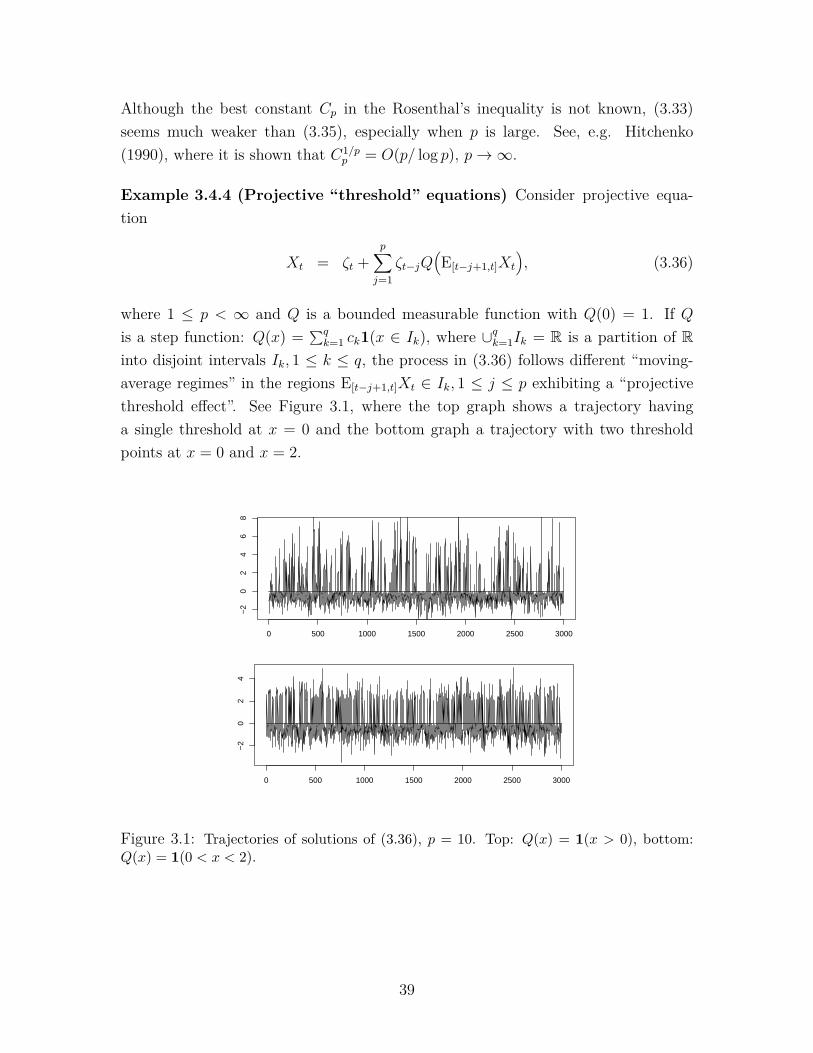
Example 3.4.4 (Projective “threshold” equations) Consider projective equa-tion
Xt = ζt +p∑j=1
ζt−jQ(E[t−j+1,t]Xt
), (3.36)
where 1 ≤ p < ∞ and Q is a bounded measurable function with Q(0) = 1. If Qis a step function: Q(x) = ∑q
k=1 ck1(x ∈ Ik), where ∪qk=1Ik = R is a partition of Rinto disjoint intervals Ik, 1 ≤ k ≤ q, the process in (3.36) follows different “moving-average regimes” in the regions E[t−j+1,t]Xt ∈ Ik, 1 ≤ j ≤ p exhibiting a “projectivethreshold effect”. See Figure 3.1, where the top graph shows a trajectory havinga single threshold at x = 0 and the bottom graph a trajectory with two thresholdpoints at x = 0 and x = 2.
0 500 1000 1500 2000 2500 3000
−2
02
46
8
0 500 1000 1500 2000 2500 3000
−2
02
4
Figure 3.1: Trajectories of solutions of (3.36), p = 10. Top: Q(x) = 1(x > 0), bottom:Q(x) = 1(0 < x < 2).
39
3.5 Simulations
Solutions of projective equations can be easily simulated using a truncated expansionX
(M)t = ∑
t−M≤s≤t gs,tζs instead of infinite series in (3.1). We chose the truncationlevel M equal to the sample size M = n = 3000 in the subsequent simulations. Thecoefficients gs,t of projective equations are computed very fast from recurrent formula(3.22) and simulated values ζs,−M ≤ s ≤ n. The innovations were taken standardnormal. For better comparisons, we used the same sequence ζs,−M ≤ s ≤ n in allsimulations.
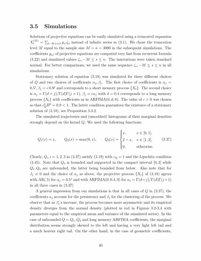
Stationary solution of equation (3.18) was simulated for three different choicesof Q and two choices of coefficients αj, βj. The first choice of coefficients is αj =0.5j, βj = c 0.9j and corresponds to a short memory process Xt. The second choiceis αj = Γ(d+ j)/Γ(d)Γ(j + 1), βj = cαj with d = 0.4 corresponds to a long memoryprocess Xt with coefficients as in ARFIMA(0, d, 0). The value of c > 0 was chosenso that c2
QB2 = 0.9 < 1. The latter condition guarantees the existence of a stationary
solution of (3.18), see Proposition 3.3.2.The simulated trajectories and (smoothed) histograms of their marginal densities
strongly depend on the kernel Q. We used the following functions:
Q1(x) = x, Q2(x) = max(0, x), Q3(x) =
x, x ∈ [0, 1],2− x, x ∈ [1, 2],0, otherwise.
(3.37)
Clearly, Qi, i = 1, 2, 3 in (3.37) satisfy (3.19) with cQ = 1 and the Lipschitz condition(3.45). Note that Q3 is bounded and supported in the compact interval [0, 2] whileQ1, Q2 are unbounded, the latter being bounded from below. Also note that forβj ≡ 0 and the choice of αj as above, the projective process Xt of (3.18) agreeswith AR(.5) for αj = 0.5j and with ARFIMA(0, 0.4, 0) for αj = Γ(d+j)/Γ(d)Γ(j+1)in all three cases in (3.37)
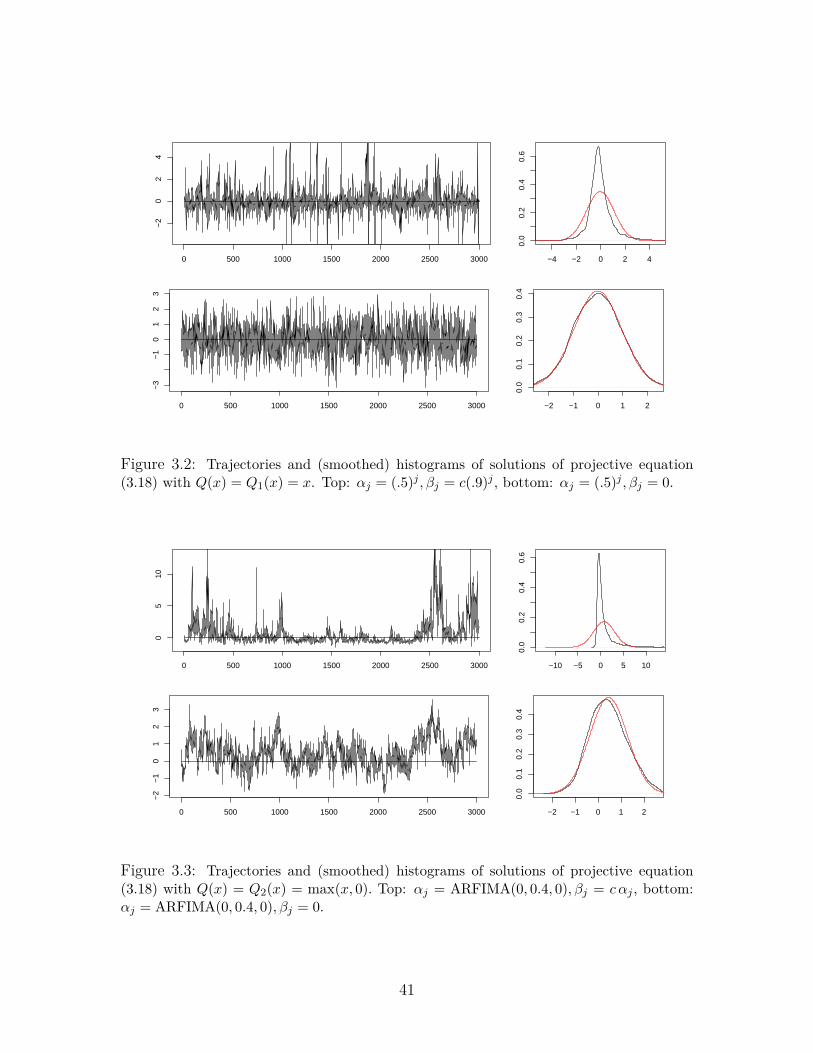
A general impression from our simulations is that in all cases of Q in (3.37), thecoefficients αj account for the persistence and βj for the clustering of the process. Weobserve that as βj’s increase, the process becomes more asymmetric and its empiricaldensity diverges from the normal density (plotted in red in Figures 3.2-3.4 withparameters equal to the empirical mean and variance of the simulated series). In thecase of unbounded Q = Q1, Q2 and long memory ARFIMA coefficients, the marginaldistribution seems strongly skewed to the left and having a very light left tail anda much heavier right tail. On the other hand, in the case of geometric coefficients,
40
0 500 1000 1500 2000 2500 3000
−2
02
4
−4 −2 0 2 4
0.0
0.2
0.4
0.6
0 500 1000 1500 2000 2500 3000
−3
−1
01
23
−2 −1 0 1 2
0.0
0.1
0.2
0.3
0.4
Figure 3.2: Trajectories and (smoothed) histograms of solutions of projective equation(3.18) with Q(x) = Q1(x) = x. Top: αj = (.5)j , βj = c(.9)j , bottom: αj = (.5)j , βj = 0.
0 500 1000 1500 2000 2500 3000
05
10
−10 −5 0 5 10
0.0
0.2
0.4
0.6
0 500 1000 1500 2000 2500 3000
−2
−1
01
23
−2 −1 0 1 2
0.0
0.1
0.2
0.3
0.4
Figure 3.3: Trajectories and (smoothed) histograms of solutions of projective equation(3.18) with Q(x) = Q2(x) = max(x, 0). Top: αj = ARFIMA(0, 0.4, 0), βj = c αj , bottom:αj = ARFIMA(0, 0.4, 0), βj = 0.
41
0 500 1000 1500 2000 2500 3000
−2
02
46
−6 −4 −2 0 2 4 6
0.0
0.1
0.2
0.3
0.4
0.5
0 500 1000 1500 2000 2500 3000
02
46
8
−1.5 −0.5 0.0 0.5 1.0 1.5
0.0
0.5
1.0
1.5
2.0
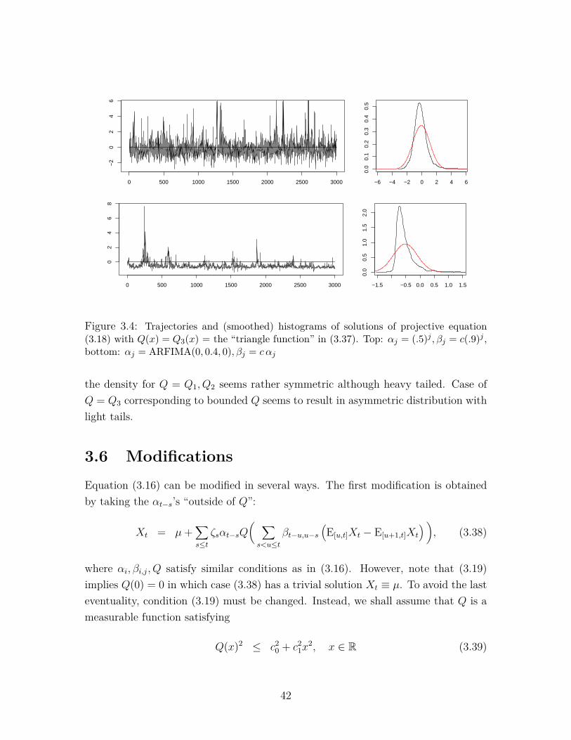
Figure 3.4: Trajectories and (smoothed) histograms of solutions of projective equation(3.18) with Q(x) = Q3(x) = the “triangle function” in (3.37). Top: αj = (.5)j , βj = c(.9)j ,bottom: αj = ARFIMA(0, 0.4, 0), βj = c αj
the density for Q = Q1, Q2 seems rather symmetric although heavy tailed. Case ofQ = Q3 corresponding to bounded Q seems to result in asymmetric distribution withlight tails.
3.6 Modifications
Equation (3.16) can be modified in several ways. The first modification is obtainedby taking the αt−s’s “outside of Q”:
Xt = µ+∑s≤t
ζsαt−sQ( ∑s<u≤t
βt−u,u−s(E[u,t]Xt − E[u+1,t]Xt
)), (3.38)
where αi, βi,j, Q satisfy similar conditions as in (3.16). However, note that (3.19)implies Q(0) = 0 in which case (3.38) has a trivial solution Xt ≡ µ. To avoid the lasteventuality, condition (3.19) must be changed. Instead, we shall assume that Q is ameasurable function satisfying
Q(x)2 ≤ c20 + c2
1x2, x ∈ R (3.39)
42
for some c0, c1 ≥ 0. Denote
KQ := c20
∞∑k=0
c2k1
∞∑i=0
α2i
∞∑j1=1
α2i+j1β
2i,j1 · · ·
∞∑jk=1
α2i+j1+···+jkβ
2i+j1+···+jk−1,jk
.
Proposition 3.6.1 can be proved similarly to Theorem 3.3.1 and its proof is omitted.
Proposition 3.6.1 (i) Assume condition (3.39) and
KQ < ∞. (3.40)
Then there exists a unique solution Xt of (3.38), which is written as a projectivemoving average of (3.7) with coefficients gt−k,t recursively defined as
gt−k,t := αkQ( k−1∑i=0
βi,k−iζt−igt−i,t
), k = 1, 2, . . . , gt,t := α0Q(0).
(ii) In the case of linear function Q(x) = c0 + c1x, condition (3.40) is also necessaryfor the existence of a solution of (3.38).
Remark 3.6.1 Let A2k := ∑∞
i=k α2i and |βi,j| ≤ β. Then
KQ ≤ c20
∞∑k=0
(c1β)2k∞∑i=0
α2i
∞∑j1=1
α2i+j1 · · ·
∞∑jk=1
α2i+j1+···+jk ≤ c2
0
∞∑k=0
(c1β)2kA20A
21 . . . A
2k.
Hence, A2 = A20 < ∞ and β < ∞ imply KQ < ∞, for any c0, c1, β; see the proof of
Proposition 3.3.2.
Projective stochastic equations (3.16) and (3.38) can be further modified by in-cluding projections of lagged variables. Consider the following extension of (3.16):
Xt = µ+ ∑s≤t
ζsQ(αt−s +
t−1∑u=s+1
βt−1−u,u−s(E[u,t−1]Xt−1 − E[u+1,t−1]
)Xt−1
), (3.41)
where αi, βi,j, Q are the same as in (3.16) and the only new feature is that t isreplaced by t − 1 in the inner sum on the r.h.s. of the equation. This fact allowsto study nonstationary solutions of (3.41) with a given projective initial conditionXt = X0
t , t ≤ 0 and the convergence of Xt to the equilibrium as t → ∞; however,we shall not pursue this topic in the present paper. The following proposition is asimple extension of Theorem 3.3.1 and its proof is omitted.
43
Proposition 3.6.2 Let αi, βi,j, Q satisfy the conditions of Theorem 3.3.1, including(3.19) and (3.21). Then there exists a unique solution Xt of (3.41), which is writtenas a projective moving average of (3.7) with coefficients gt−k,t recursively defined asgt−k,t := Q(αk), k = 0, 1 and
gt−k,t := Q(αk +
k−2∑i=0
βi,k−1−iζt−1−igt−1−i,t−1), k ≥ 2.
Finally, consider a projective equation (3.13) with µt ≡ 0 and kernels Qs,t =Qt−s(xs+1,t−1, . . . , xs+1,s) depending on t− s real variables, where Q0 = 1 and
Qj(x1, . . . , xj) = d(x1)1 · d(x2) + 1
2 · d(x3) + 23 . . .
d(xj) + j − 1j
, (3.42)
j ≥ 1, where d(x), x ∈ R is a measurable function taking values in the interval(−1/2, 1/2). More explicitly,
Xt =∞∑j=0
Qj
(E[t−j+1,t−1]Xt−1,E[t−j+1,t−2]Xt−2, . . . ,E[t−j+1,t−j]Xt−j
)ζt−j, (3.43)
where E[t−j+1,t−j]Xt−j = EXt = 0. Note that when d(x) = d is constant, Xt(3.43) is a stationary ARFIMA(0, d, 0) process. Time-varying fractionally integratedprocesses with deterministic coefficients of the form (3.42) were studied in Philippeet al. (2006), Philippe et al. (2008). We expect that (3.43) feature a “random”memory intensity depending on the values of the process. A rigorous study of longmemory properties of this model does not seem easy. On the other hand, solvabilityof (3.43) can be established similarly to the previous cases (see below).
Proposition 3.6.3 Let d(x) be a measurable function taking values in (−1/2, 1/2)and such that supx∈R d(x) ≤ d, where d ∈ (0, 1/2). Then there exists a uniquestationary solution Xt of (3.43), which is written as a projective moving averageof (3.7) with coefficients gs,t recursively defined as gt,t := 1 and
gs,t := Qt−s( ∑s<u≤t−1
ζugu,t−1,∑
s<u≤t−2ζugu,t−2, . . . , 0
), s < t, (3.44)
with Qt−s defined at (3.42).
Proof. Note that supx1,...,xj∈R |Qj(x1, . . . , xj)| ≤ Γ(d + j)/Γ(d)Γ(j) =: ψj and∑∞j=0 ψ
2j < ∞. Therefore the gs,t’s in (3.44) satisfy ∑
s≤t Eg2s,t < ∞ for any t ∈ Z.
The rest of the proof is analogous as the case of Theorem 3.3.1.
44
3.7 Long memory
In this section we study long memory properties (the decay of covariance and partialsums’ limits) of projective equations (3.16) and (3.38) in the case when the coefficientsαj’s decay slowly as jd−1, 0 < d < 1/2.
Theorem 3.7.1 Let Xt be the solution of projective equation (3.16) satisfying theconditions of Theorem 3.3.1 and µ = EXt = 0. Assume, in addition, that Q is aLipschitz function, viz., there exists a constant cL > 0 such that
|Q(x)−Q(y)| < cL|x− y|, x, y ∈ R (3.45)
and that there exist κ > 0 and 0 < d < 1/2 such that
bj := Q(αj) ∼ κ jd−1, j →∞ (3.46)
and
βj := max0≤i<j
|βi,j−i| = o(bj), j →∞. (3.47)
Then, as t→∞
EX0Xt ∼∞∑k=0
bkbt+k ∼ κ2dt
2d−1, (3.48)
where κ2d := κ2B(d, 1− d) and B(d, 1− d) is beta function. Moreover, as n→∞
n−1/2−d[nτ ]∑t=1
Xt −→D[0,1] cκ,dBH(τ), (3.49)
where BH is a fractional Brownian motion with parameter H = d+(1/2) and varianceEB2
H(t) = t2H and c2κ,d := κ2B(d,1−d)
d(1+2d) .
Proof. Let us note that the statements (3.48) and (3.49) are well-known whenβi,j ≡ 0, in which case Xt coincides with the linear process Yt := ∑
s≤t bt−sζs, see,e.g., Giraitis et al. (2012), Proposition 3.2.1 and Corollary 4.4.1.
The natural idea of the proof is to approximate Xt by the linear process Yt.
45
For t ≥ 0, k ≥ 0, denote
rXt := EX0Xt =∑s≤0
E[gs,0 gs,t], rYt := EY0Yt =∑s≤0
b−sbt−s,
ϕt−k,t := gt−k,t − bk = Q(αk +
k−1∑i=0
βi,k−iζt−igt−i,t
)−Q(αk).
Then
rXt − rYt =∑s≤0
E[(b−s + ϕs,0)(bt−s + ϕs,t)− b−sbt−s]
=∑s≤0
b−sE[ϕs,t] +∑s≤0
bt−sE[ϕs,0] +∑s≤0
E[ϕs,0 ϕs,t] =:3∑i=1
ρi,t.
Using (3.45) we obtain
|Eϕt−k,t|2 ≤ Eϕ2t−k,t ≤ c2
LE( k−1∑i=0
βi,k−iζt−igt−i,t
)2
= c2L
( k−1∑i=0
β2i,k−iEg2
t−i,t
)
≤ β2kc
2L
( ∞∑i=0
Eg2t−i,t
)≤ β2
kc2LKQ.
This and condition (3.47) imply that
|Eϕt−k,t|+ E1/2ϕ2t−k,t ≤ δkk
d−1, ∀ t, k ≥ 0,
where δk → 0 (k →∞). Therefore for any t ≥ 1
|ρ1,t| ≤ C∞∑k=1
kd−1(t+ k)d−1δt+k ≤ Cδ′tt2d−1,
|ρ2,t| ≤ C∞∑k=1
kd−1δk(t+ k)d−1 ≤ Cδ′tt2d−1,
|ρ3,t| ≤∑s≤t
E1/2[ϕ2s,0] E1/2[ϕ2
s,t] ≤ C∞∑k=1
kd−1(t+ k)d−1δkδt+k ≤ Cδ′tt2d−1,
where δ′k → 0 (k →∞). This proves (3.48).To show (3.49), consider Zt := Xt − Yt = ∑
u≤t ϕu,tζu, t ∈ Z. By stationarity of
46
Zt, for any s ≤ t we have
Cov(Zt, Zs) =∑u≤0
E[ϕu,0 ϕu,t−s] ≤∑u≤0
E1/2[ϕ2u,0] E1/2[ϕ2
u,t−s] = o((t− s)2d−1),
see above, and therefore E(∑n
t=1 Zt)2
= o(n2d+1), implying
n−d−(1/2)[nτ ]∑t=1
Xt = n−d−(1/2)[nτ ]∑t=1
Yt + op(1).
Therefore partial sums of Xt and Yt tend to the same limit cκ,dBH(τ), in thesense of weak convergence of finite dimensional distributions. The tightness in D[0, 1]follows from (3.48) and the Kolmogorov criterion. Theorem 3.7.1 is proved.
A similar but somewhat different approximation by a linear process applies in thecase of projective equations of (3.38). Let us discuss a special case of βi,j:
βi,j = 1, for all i = 0, 1, . . . , j = 1, 2, . . . . (3.50)
Note that for such βi,j,∑s<u≤t βt−u,u−s(E[u,t] − E[u+1,t])Xt = E[s+1,t]Xt, s < t and
the corresponding projective equation (3.38) with µ = 0, αi = bi coincides with(3.5). Recall that for bounded βi,j’s as in (3.50), condition (3.39) on Q together with∑∞i=0 α
2i < ∞ guarantee the existence of the stationary solution Xt (see Remark
3.6.1). We shall also need the following additional condition:
E(Q(E[s,0]X0)−Q(X0)
)2→ 0, as s→ −∞. (3.51)
Since E(E[s,0]X0 − X0
)2→ 0, s → −∞, so (3.51) is satisfied if Q is Lipschitz, but
otherwise conditions (3.51) and (3.39) allow Q to be even discontinuous. Denote
c2Q,d :=
(E[Q(X0)]
)2B(d, 1− d).
Theorem 3.7.2 Let Xt be the solution of projective equation (3.38) with µ =0, βi,j as in (3.50), Q satisfying (3.39) and
αk ∼ kd−1, k →∞, ∃ 0 < d < 1/2. (3.52)
In addition, let (3.51) hold. Then
EX0Xt ∼ c2Q,dt
2d−1, t→∞ (3.53)
47
and
n−1/2−d[nτ ]∑t=1
Xt −→D[0,1] c′Q,dBH(τ), c′Q,d := cQ,d/(d(1 + 2d)1/2. (3.54)
Proof. Similarly as in the proof of the previous theorem, let Yt := ∑s≤t bt−sζs,
bk := αkE[Q(X0)], rXt := EX0Xt, rYt := EY0Yt, t ≥ 0. Relation (3.53) follows from
rXt − rYt = o(t2d−1), t→∞. (3.55)
We have Xt = ∑s≤t gs,tζs, gs,t = αt−sQ(E[s+1,t]Xt), EX2
t = ∑s≤t Eg2
s,t < ∞ andE[Q(E[s+1,t]Xt)2] ≤ c2
0+c21E(E[s+1,t]Xt)2 ≤ c2
0+c21EX2
t < C. Decompose rXt = rX1,t+rX2,t,where
rX1,t :=∑s≤0
αsαt+sE[Q(E[s+1,0]X0)] E[Q(E[1,t]Xt)], rX2,t :=∑s≤0
αsαt+sγs,t,
and where
|γs,t| :=∣∣∣E[Q(E[s+1,0]X0)
Q(E[s+1,t]Xt)−Q(E[1,t]Xt)
]∣∣∣ ≤ γ1/21,s γ
1/22,s,t.
Here, γ1,s := E[Q2(E[s+1,0]X0)] ≤ C, see above, while
|γ2,s,t| := E[(Q(E[s+1,t]Xt)−Q(E[1,t]Xt)
)2]= E
[(Q(E[s+1−t,0]X0)−Q(E[1−t,0]X0)
)2]→ 0, t→∞ (3.56)
uniformly in s ≤ 0, according to (3.51). Hence and from (3.52) it follows that
|rX2,t| = o(t2d−1), t→∞. (3.57)
Accordingly, it suffices to prove (3.55) with rXt replaced by rX1,t. We have
rX1,t = rYt +∑s≤0
αsαt+sϕ1,s,t +∑s≤0
αsαt+sϕ2,s,t +∑s≤0
αsαt+sϕ3,s,t,
where the “remainders” ϕ1,s,t := E[Q(X0)]
E[Q(E[s+1,0]X0)] − E[Q(X0)], ϕ2,s,t :=
E[Q(X0)]
E[Q(E[1−t,0]X0)]− E[Q(X0)]
and ϕ3,s,t :=(E[Q(E[s+1,0]X0)]− E[Q(X0)]
)×(E[Q(E[1−t,0]X0)]− E[Q(X0)]
)can be estimated similarly to (3.56), leading to the
asymptotics of (3.57) for each of the three sums in the above decomposition of rX1,t.This proves (3.53).
48
Let us prove (3.54). Consider the convergence of one-dimensional distributionsfor τ = 1, viz.,
n−d−1/2SXn → N (0, σ2), σ = c′Q,d, (3.58)
where SXn := ∑nt=1Xt. Then (3.58) follows from
E(SXn − SYn )2 = o(n1+2d), (3.59)
where SYn := ∑nt=1 Yt and Yt is as above. We have
E(SXn − SYn )2 = E(∑s≤n
ζsn∑
t=1∨sαt−sQs,t
)2
=∑s≤n
n∑t1,t2=1∨s
αt1−sαt2−sE[Qs,t1Qs,t2 ], (3.60)
where Qs,t := Q(E[s+1,t]Xt
)− E[Q(X0)]. Let us prove that uniformly in s ≤ t1
E[Qs,t1Qs,t2 ] = o(1), as t2 − t1 →∞. (3.61)
We have for s ≤ t1 ≤ t2 that
E[Qs,t1Qs,t2 ] = E[Qs,t1
Q(E[s+1,t2]Xt2
)− E[Q(X0)]
]= E[Qs,t1 ]
E[Q(E[t1+1,t2]Xt2
)]− E[Q(X0)]
+ E
[Qs,t1
Q(E[s+1,t2]Xt2
)−Q
(E[t1+1,t2]Xt2
)]=: ψ′s,t1,t2 + ψ′′s,t1,t2 ,
where we used the fact that Qs,t1 and Q(E[t1+1,t2]Xt2
)are independent. Here, thanks
to (3.51), we see that |ψ′s,t1,t2| ≤ E1/2[Q2s,t1 ] E1/2
[Q(E[t1−t2+1,0]X0
)− Q(X0)
2]≤
CE1/2[Q(E[t1−t2+1,0]X0
)−Q(X0)
2]→ 0 uniformly in s ≤ t1 ≤ t2 as t2 − t1 →∞.
The same is true for |ψ′′s,t1,t2| since it is completely analogous to (3.56). This proves(3.61). Next, with (3.60) in mind, split E(SXn − SYn )2 =: Tn = T1,n + T2,n, where
T1,n :=∑s≤n
n∑t1,t2=1∨s
1(|t1 − t2| > K) . . . , T2,n :=∑s≤n
n∑t1,t2=1∨s
1(|t1 − t2| ≤ K) . . . ,
where K is a large number. By (3.61), for any ε > 0 we can find K > 0 such thatsups≤t1<t2:t2−t1>K |E[Qs,t1Qs,t2 ]| < ε and therefore
|T1,n| < ε∑s≤n
n∑t1,t2=1∨s
|αt1−sαt2−s| ≤ Cεn∑
t1,t2=1|rt1−t2| ≤ Cεn1+2d
49
holds for all n > 1 large enough, where rt := ∑∞i=0 |αiαt+i| = O(t2d−1) in view of
(3.52). On the other hand, |T2,n| ≤ CKn = o(n1+2d) for any K < ∞ fixed. Then(3.59) follows, implying the finite-dimensional convergence in (3.54). The tightnessin (3.54) follows from (3.53) and the Kolmogorov criterion, similarly as in the proofof Theorem 3.7.1. Theorem 3.7.2 is proved.
Remark 3.7.1 Shao and Wu (2006) discussed partial sums limits of fractionallyintegrated nonlinear processes Yt = (1 − L)−dut, t ∈ Z, where LXt = Xt−1 is thebackward shift, (1− L)d = ∑∞
j=0 ψj(d)Lj, d ∈ (−1, 1) is the fractional differentiationoperator, and ut is a causal Bernoulli shift:
ut = F (. . . , ζt−1, ζt), t ∈ Z (3.62)
in i.i.d. r.v.’s ζt, t ∈ Z. The weak dependence condition on ut (3.62), analogousto (3.11) and guaranteeing the weak convergence of normalized partial sums of Yttowards a fractional Brownian motion, is written in terms of projections P0ut =(E[0,t] − E[1,t])ut:
Ω(q) :=∞∑t=1‖P0ut‖q < ∞, (3.63)
where ‖ξ‖q := E1/q|ξ|q and q = 2 for 0 < d < 1/2; see Theorem. 2.1 in Shao andWu (2006), also Wu and Min (2005), Wu (2005). The above mentioned papers verify(3.63) for several classes of Bernoulli shifts. It is of interest to verify (3.63) forprojective moving averages. For Xt of (3.1) and 0 < d < 1/2, ut := (1 − L)dXt =∑s≤t ζsGs,t is a well-defined projective moving average with coefficients
Gs,t :=∑s≤v≤t
ψt−v(d)gs,v, s ≤ t,
see Proposition 3.2.2. For concreteness, let gs,t = ψt−s(−d)Q(E[s+1,t]Xt) as in Theo-rem 3.7.2 with αj = ψj(−d). We have Ω(2) = ∑∞
t=1 ‖G0,t‖2, where
‖G0,t‖22 = E
[ t∑v=0
ψt−v(d)ψv(−d)Q(E[1,v]Xv)]2
= E[ t−1∑v=0
ψt−v(d)ψv(−d)Qv,t
]2, (3.64)
where Qv,t := Q(E[1,v]Xv) − Q(E[1,t]Xt) and we used ∑tv=0 ψt−v(d)ψv(−d) = 0, t ≥ 1
in the last equality. Note that ψt−v(d)ψv(−d) < 0 have the same sign and Qv,t ≈Q(Xv)−Q(Xt) are not negligible in (3.64). Therefore we conjecture that ‖G0,t‖2
2 =O(∑t−1
v=0 |ψt−v(d)ψv(−d)|)2
= O(t−2(1−d)) and hence Ω(2) =∞ for 0 < d < 1/2. The
50

above argument suggests that projective moving averages posses a different “memorymechanism” from fractionally integrated processes in Shao and Wu (2006).
51
Chapter 4
A nonlinear model for longmemory conditionalheteroscedasticity
Abstract. We discuss a class of conditionally heteroscedastic time series modelssatisfying the equation rt = ζtσt, where ζt are standardized i.i.d. r.v.’s and theconditional standard deviation σt is a nonlinear function Q of inhomogeneous linearcombination of past values rs, s < t with coefficients bj. The existence of stationarysolution rt with finite pth moment, 0 < p < ∞ is obtained under some conditionson Q, bj and the pth moment of ζ0. Weak dependence properties of rt are studied,including the invariance principle for partial sums of Lipschitz functions of rt. Inthe case when Q is the square root of a quadratic polynomial, we prove that rt canexhibit a leverage effect and long memory, in the sense that the squared process r2
t haslong memory autocorrelation and its normalized partial sums process converges to afractional Brownian motion. The results are extended to a generalized model wherethe conditional variance satisfies an AR(1) equation σ2
t = Q2(a+∑∞j=1 bjrt−j
)+γσ2
t−1.We also provide another condition for the existence of higher moments of rt whichdoes not include the Rosenthal constant. A simulated trajectories and histograms ofmarginal density of σt for different values of γ are presented.
52
4.1 Introduction
A class of conditionally heteroscedastic ARCH-type processes is defined from a stan-dardized i.i.d. sequence ζt, t ∈ Z as solutions of stochastic equation
rt = ζtσt, σt = V (rs, s < t), (4.1)
where V (x1, x2, . . . ) is some function of x1, x2, . . . . The present chapter discusses aclass of models (4.1) with V of the form
V (x1, x2, . . . ) = Q(a+∞∑j=1
bjxj), (4.2)
where Q(x), x ∈ R is a (nonlinear) function of a single real variable x ∈ R whichmay be separated from zero by a positive constant: Q(x) ≥ c > 0, x ∈ R. LinearQ(x) = x corresponds to the LARCH model (2.11). Probably, the most interestingnonlinear case of Q in (4.2) is
Q(x) =√c2 + x2, (4.3)
where c ≥ 0 is a parameter. In the latter case, the model is described by equations
rt = ζtσt, σt =√√√√c2 +
(a+
∑s<t
bt−srs
)2. (4.4)
Note that σt ≥ c ≥ 0 in (4.4) is nonnegative and separated from 0 if c > 0. Particularcases of volatility forms in (4.4) are:
σt =√c2 + (a+ brt−1)2 ( Engle (1990) asymmetric ARCH(1)), (4.5)
σt =√√√√c2 +
(a+ b
p
p∑j=1
rt−j)2, (4.6)
σt =∣∣∣a+
∞∑j=1
bjrt−j∣∣∣ (Q(x) = |x|), (4.7)
σt =√c2 + (a+ b((1− L)−d − 1)rt)2. (4.8)
In (4.5)-(4.8), a, b, c are real parameters, p ≥ 1 an integer, Lxt = xt−1 is the backwardshift, and (1 − L)−dxt = ∑∞
j=0 ϕjxt−j, ϕj = Γ(d + j)/Γ(d)Γ(j + 1), ϕ0 = 1 is thefractional integration operator, 0 < d < 1/2. The squared volatility (conditionalvariance) σ2
t in (4.5)-(4.8) and (4.4) is a quadratic form in lagged returns rt−1, rt−2, . . .
53
and hence represent particular cases of Sentana (1995) Quadratic ARCH (QARCH)model with p = ∞. It should be noted, however, that the first two conditionalmoments do not determine the unconditional distribution. Particularly, (4.1) with(4.4) generally is a different process from Sentana (1995) QARCH process, the latterbeing defined as a solution of a linear random-coefficient equation for rt in contrastto the nonlinear equation in (4.1). See also Example 4.2.2 below.
The model in (4.1)-(4.2) can be generalized by including the lagged volatilitiesfrom the past, in particular
rt = ζtσt, σ2t = Q2
(a+
∞∑j=1
bjrt−j
)+ γσ2
t−1, (4.9)
where 0 ≤ γ < 1 is a parameter. The inclusion of lagged σ2t−1 in (4.9) helps to reduce
very sharp peaks and clustering of volatility which occur in trajectory of (4.1)-(4.2)with (4.3) near the threshhold c > 0 (see Figure 4.1). The generalization from (4.1)-(4.2) to (4.9) is similar to that from ARCH to GARCH models, see Engle (1982),Bollerslev (1986), particularly, (4.9) with Q(x) of (4.3) and bj = 0, j ≥ 2 reduces tothe Asymmetric GARCH(1,1) of Engle (1990), see Example 4.6.1.
Let us describe the main results of this chapter. Section 4.2 obtains sufficientconditions on Q, bj and |µ|p := E|ζ0|p for the existence of stationary solution of (4.1)-(4.2) with finite moment E|rt|p <∞, p > 0. We use the fact that the above equationscan be reduced to the “nonlinear moving-average” equation
Xt =∑s<t
bt−sζsQ(a+Xs)
for linear form Xt := ∑s<t bt−srs in (4.2), and vice-versa. Section 4.3 aims at pro-
viding weak dependence properties of model (4.1)-(4.2), in particular, the invarianceprinciple for Lipschitz functions of rt and Xt, under the assumption that bj aresummable and decay as j−γ with γ > 1. Section 4.4 discusses long memory prop-erty of the quadratic model in (4.4). For bj ∼ βjd−1, j → ∞, 0 < d < 1/2 asin (4.8), we prove that the squared process r2
t has long memory autocorrelationsand its normalized partial sums process tend to a fractional Brownian motion withHurst parameter H = d + 1/2 (Theorem 4.4.2). Section 4.5 establishes the leverageeffect in spirit of Giraitis et al. (2004), viz., the fact that the “leverage function”hj := Cov(σ2
t , rt−j), j ≥ 1 of model (4.4) takes negative values provided the coeffi-cients a and bj have opposite signs. Finally, Section 4.6 extends the results of previoussections to a more general class of volatility forms in (4.9) that include lagged volatil-
54
ity from the past σ2t−1. In addition, another condition for the existence of higher
moments of rt which does not include the Rosenthal constant is obtained in Theorem4.6.2. Simulated trajectories and histograms of marginal density for different valuesof parameter γ are presented in Section 4.7.
Notation. In what follows, C,C(. . . ) denote generic constants, possibly dependenton the variables in brackets, which may be different at different locations. at ∼ bt (t→∞) is equivalent to limt→∞ at/bt = 1.
4.2 Stationary solution
This section discusses the existence of a stationary solution of (4.1)-(4.2), viz.,
rt = ζtQ(a+
∑s<t
bt−srs), t ∈ Z. (4.10)
DenoteXt :=
∑s<t
bt−srs. (4.11)
Then rt in (4.10) can be written as rt = ζtQ(a + Xt) where (4.11) formally satisfiesthe following equation:
Xt =∑s<t
bt−sζsQ(a+Xs). (4.12)
Below we give rigorous definitions of solutions of (4.10) and (4.12) and a statement(Proposition 4.2.2) justifying (4.12) and the equivalence of (4.10) and (4.12).
In this section we consider a general case of (4.10)-(4.12) when the innovationsmay have infinite variance. More precisely, we assume that ζt, t ∈ Z are i.i.d.r.v.’s with finite moment |µ|p := E|ζt|p < ∞, p > 0. We use the following momentinequality.
Proposition 4.2.1 Let Yj, j ≥ 1 be a sequence of r.v.’s such that E|Yj|p < ∞ forsome p > 0 and the sum on the r.h.s. of (4.13) converges. If p > 1 we additionallyassume that Yj is a martingale difference sequence: E[Yj|Y1, . . . , Yj−1] = 0, j =2, 3, . . . . Then there exists a constant Kp depending only on p and such that
E∣∣∣ ∞∑j=1
Yj∣∣∣p ≤ Kp
∑∞j=1 E|Yj|p, 0 < p ≤ 2,(∑∞j=1(E|Yj|p)2/p
)p/2, p > 2.
(4.13)
Remark 4.2.1 In the sequel, we shall refer toKp in (4.13) as the Rosenthal constant.For 0 < p ≤ 1 and p = 2, inequality (4.13) holds with Kp = 1, and for 1 < p < 2, it
55
is known as von Bahr and Esséen inequality, see von Bahr and Esséen (1965), whichholds with Kp = 2. For p > 2, inequality (4.13) is a consequence of the Burkholderand Rosenthal inequality (see Burkholder (1973), Rosenthal (1970), also Giraitis et al.(2012), Lemma 2.5.2). Osekowski (2012) proved that K1/p
p ≤ 2(3/2)+(1/p)(p4 +1)1/p(1+
plog(p/2)
), in particular, K1/4
4 ≤ 27.083. See also Hitchenko (1990).
Let us give some formal definitions. Let Ft = σ(ζs, s ≤ t), t ∈ Z be the sigma-fieldgenerated by ζs, s ≤ t. A random process ut, t ∈ Z is called adapted (respectively,predictable) if ut is Ft-measurable for each t ∈ Z (respectively, ut is Ft−1-measurablefor each t ∈ Z). Define
Bp :=
∑∞j=1 |bj|p, 0 < p < 2,(∑∞j=1 b
2j
)p/2, p ≥ 2.
(4.14)
Definition 4.2.1 Let p > 0 be arbitrary.(i) By Lp-solution of (4.10) we mean an adapted process rt, t ∈ Z with E|rt|p <∞such that for any t ∈ Z the series ∑s<t bt−srs converges in Lp and (4.10) holds.(ii) By Lp-solution of (4.12) we mean a predictable process Xt, t ∈ Z with E|Xt|p <∞ such that for any t ∈ Z the series ∑s<t bt−sζsQ(a+Xs) converges in Lp and (4.12)holds.
Let Q(x), x ∈ R be a Lipschitz function, i.e., there exists LipQ > 0 such that
|Q(x)−Q(y)| ≤ LipQ|x− y|, x, y ∈ R. (4.15)
Note (4.15) implies the bound
Q2(x) ≤ c21 + c2
2x2, x ∈ R, (4.16)
where c1 ≥ 0, c2 ≥ LipQ and c2 can be chosen arbitrarily close to LipQ; in particular,(4.16) holds with c2
2 = (1 + ε2)Lip2Q, c
21 = Q2(0)(1 + ε−2), where ε > 0 is arbitrarily
small.
Proposition 4.2.2 Let Q be a measurable function satisfying (4.16) with some ci ≥0, i = 1, 2 and ζt be an i.i.d. sequence with |µ|p = E|ζ0|p < ∞ and satisfyingEζ0 = 0 for p > 1. In addition, assume Bp <∞.(i) Let Xt be a stationary Lp-solution of (4.12). Then rt := ζtQ(a + Xt) is astationary Lp-solution of (4.10) and
E|rt|p ≤ C(1 + E|Xt|p). (4.17)
56
Moreover, for p > 1, rt,Ft, t ∈ Z is a martingale difference sequence with
E[rt|Ft−1] = 0, E[|rt|p|Ft−1] = |µ|p∣∣∣Q(a+
∑s<t
bt−srs)|p. (4.18)
(ii) Let rt be a stationary Lp-solution of (4.10). Then Xt in (4.11) is a stationaryLp-solution of (4.12) such that
E|Xt|p ≤ CE|rt|p. (4.19)
Moreover, for p ≥ 2
E[XtX0] = Er20
∞∑s=1
bt+sbs, t = 0, 1, . . . . (4.20)
Remark 4.2.2 Let p ≥ 2 and |µ|p < ∞, then by inequality (4.13), rt being astationary Lp-solution of (4.10) is equivalent to rt being a stationary L2-solution of(4.10) with E|r0|p <∞. Similarly, if Q and ζt satisfy the conditions of Proposition4.2.2 and p ≥ 2, then Xt being a stationary Lp-solution of (4.12) is equivalent toXt being a stationary L2-solution of (4.12) with E|X0|p <∞.
Proof of Proposition 4.2.2. (i) Since Xt is predictable and Q satisfies (4.16) so
E|rt|p = |µ|pE|Q(a+Xt)|p
≤ |µ|pE|c21 + c2
2(a+Xt)2|p/2
≤ C(1 + E|Xt|p) < C <∞,
proving (4.17). Moreover, if p > 1 then E[rt|Ft−1] = 0 is a stationary martingaledifference sequence. Hence by Proposition 4.2.1, the series in (4.11) converges in Lp
and satisfies
E|Xt|p ≤ C
∑∞j=1 |bj|p, 0 < p ≤ 2(∑∞j=1 b
2j
)p/2, p > 2
= CBp < ∞.
In particular, ζtQ(a+∑s<t bt−srs) = ζtQ(a+Xt) = rt by the definition of rt. Hence,
rt is a Lp-solution of (4.10). Stationarity of rt follows from stationarity of Xt.Relations (4.18) follow from E[ζt|Ft−1] = 0, E[|ζt|p|Ft−1] = |µ|p, p > 1, and the
fact that Xt is Ft−1-measurable.(ii) Since rt is a Lp-solution of (4.10), so rt = ζtQ(a + Xt) with Xt defined in(4.11), and Xt satisfy (4.12), where the series converges in Lp. Also note that Xt
57
is predictable. Hence, Xt is a Lp-solution of (4.12). By (4.16),
E|rt|p = |µ|pE|Q(a+Xt)|p ≤ |µ|pE|c21 + c2
2(a+Xt)2|p/2 ≤ C(1 + E|Xt|p) < C.
It also readily follows that, for p > 1, rt,Ft, t ∈ Z is a martingale differencesequence. Hence, by the moment inequality in (4.13),
E|Xt|p ≤ Kp
∑∞j=1 |bj|pE|rt−j|p, 0 < p ≤ 2(∑∞j=1 b
2jE2/p|rt−j|p
)p/2, p > 2
= CBpE|rt|p, (4.21)
proving (4.19). Stationarity of Xt and (4.20) are easy consequences of the abovefacts and stationarity of rt.
The following theorem obtains a sufficient condition in (4.22) for the existenceof a stationary Lp-solution of equations (4.10) and (4.12). Condition (4.22) involvesthe pth moment of innovations, the Lipschitz constant LipQ, the sum Bp in (4.14)and the Rosenthal constant Kp in (4.13). Part (ii) of Theorem 4.2.1 shows that forp = 2, condition (4.22) is close to optimal, being necessary in the case of quadraticQ2(x) = c2
1 + c22x
2.
Theorem 4.2.1 Let the conditions of Proposition 4.2.2 be satisfied, p > 0 is arbi-trary. In addition, assume that Q satisfies the Lipschitz condition in (4.15).
(i) LetKp|µ|pLippQBp < 1. (4.22)
Then there exists a unique stationary Lp-solution Xt of (4.12) and
E|Xt|p ≤C(p,Q)|µ|pBp
1−Kp|µ|pLippQBp
, (4.23)
where C(p,Q) <∞ depends only on p and c1, c2 in (4.16).(ii) Assume, in addition, that Q2(x) = c2
1 + c22x
2, where ci ≥ 0, i = 1, 2, and µ2 =Eζ2
0 = 1. Then c22B2 < 1 is a necessary and sufficient condition for the existence of
a stationary L2-solution Xt of (4.12) with a 6= 0.
Remark 4.2.3 Condition (4.22) agrees with the contraction condition for the op-erator defined by the r.h.s. of (4.12) and acting in a suitable space of predictableprocesses with values in Lp. For the LARCH model, explicit conditions for finitenessof the pth moment were obtained in Giraitis et al. (2000), Giraitis et al. (2004) usinga specific diagram approach for multiple Volterra series. For larger values of p > 2,
58
condition (4.22) is preferable to the corresponding condition
(2p − p− 1)1/2|µ|1/pp B1/pp < 1, p = 2, 4, 6, . . . , (4.24)
in Giraitis et al. (2000), formula (2.12) for the LARCH model, since the coefficient(2p−p−1)1/2 grows exponentially with p in contrast to the bound on K1/p
p in Remark4.2.1 (see also Chapter 3, Example 3.4.3). On the other hand for p = 4 (4.24) becomes√
11|µ|1/44 B1/22 < 1 while (4.22) is satisfied if K1/4
4 |µ|1/44 B
1/22 ≤ 27.083|µ|1/44 B
1/22 < 1,
see Remark 4.2.1, which is worse than (4.24).
Proof of Theorem 4.2.1. (i) For n ∈ N define a solution of (4.12) with zero initialcondition at t ≤ −n as
X(n)t :=
0, t ≤ −n,∑t−1s=−n bt−sζsQ(a+X(n)
s ), t > −n, t ∈ Z.(4.25)
Let us show that X(n)t converges in Lp to a stationary Lp-solution Xt as n→∞.
First, let 0 < p ≤ 2. Let m > n ≥ 0. Then by inequality (4.13) for any t > −m wehave that
E|X(m)t −X(n)
t |p = Kp|µ|p ∑−m≤s<−n
|bt−s|pE|Q(a+X(m)s )|p
+∑
−n≤s<t|bt−s|pE
∣∣∣Q(a+X(n)s )−Q(a+X(m)
s )∣∣∣p
=: Kp|µ|pS ′m,n + S ′′m,n.
Let χp(n) := ∑∞j=n |bj|p. From the bound |a+ x|2 ≤ (2a2/ε) + (1 + ε)x2, valid for any
0 < ε < 1/2, x ∈ R and a ≥ 0, it follows that
∣∣∣c21 + c2
2(a+X(m)s )2)
∣∣∣p/2 ≤ cp1 + cp2|(a+X(m)s )2|p/2
≤ C(c1, c2) + cp2 (1 + ε)p/2|X(m)s |p
≤ C(c1, c2) + cp3|X(m)s |p,
59
with c3 > c2 > LipQ arbitrarily close to LipQ. Then using (4.16) we obtain
S ′m,n ≤∑
−m≤s<−n|bt−s|pE
∣∣∣c21 + c2
2(a+X(m)s )2
∣∣∣p≤ C(Q)Kp|µ|pχp(t+ n) + cp3
∑−m≤s<−n
|bt−s|pE|X(m)s −X(n)
s |p,
S ′′m,n ≤ LippQ∑
−n≤s<t|bt−s|pE
∣∣∣X(n)s −X(m)
s
∣∣∣p.Consequently,
E|X(m)t −X(n)
t |p ≤ C(Q)Kp|µ|pχp(t+ n) +Kp|µ|pcp3∑
−m≤s<t|bt−s|pE
∣∣∣X(n)s −X(m)
s
∣∣∣p.Iterating the above inequality, we obtain
E|X(m)t −X(n)
t |p ≤ C(Q)Kp|µ|pχp(t+ n) +
∞∑k=1
(Kp|µ|kcp3)k (4.26)
×∑
−m≤sk<···<s1<t
|bt−s1|p|bs1−s2|p . . . |bsk−1−sk |pχp(sk + n).
Since Kp|µ|pcp3Bp < 1 by (4.22) and sups≥1 χp(s) ≤ Bp <∞, the series on the r.h.s. of(4.26) is bounded uniformly in m,n and tends to zero as m,n→∞ by the dominatedconvergence theorem. Hence, there exist Xt, t ∈ Z such that
limn→∞
E|Xt −X(n)t |p = 0, ∀ t ∈ Z. (4.27)
Note that Xt is predictable and
E|Xt|p = limn→∞
E|X(n)t |p ≤
C(Q)Kp|µ|pBp
1−Kp|µ|pcp3Bp
≤ C(p,Q)|µ|pBp
1−Kp|µ|pLippQBp
,
where the last inequality follows by taking c3 > LipQ sufficiently close to LipQ.
60
We also have by (4.23) and (4.15) that
E∣∣∣∑s<t
bt−sζsQ(a+Xs)−t−1∑s=−n
bt−sζsQ(a+X(n)s )
∣∣∣p= E
∣∣∣ ∑s<−n
bt−sζsQ(a+Xs) +t−1∑s=−n
bt−sζs(Q(a+Xs)−Q(a+X(n)s ))
∣∣∣p≤ Kp|µ|p
∑s<−n
|bt−s|pE∣∣∣Q(a+Xs)
∣∣∣p+
∑−n≤s<t
|bt−s|pE∣∣∣Q(a+Xs)−Q(a+X(n)
s )∣∣∣p
≤ C( ∑s<−n
|bt−s|p +∑s<t
|bt−s|pE∣∣∣Xs −X(n)
s
∣∣∣p) → 0
as n→∞. Whence and from (4.25) it follows that Xt is a stationary Lp-solutionof (4.12) satisfying (4.23).
To show the uniqueness of stationary Lp-solution of (4.12), let X ′t, X ′′t be twosuch solutions of (4.12), and mp(t) := E|X ′t−X ′′t |p. Then supt∈Zmp(t) ≤M <∞ andmp(t) ≤ Kp|µ|pLippQ
∑s<t |bt−s|pmp(s) follows by (4.15). Iterating the last equation we
obtain that mp(t) ≤ (Kp|µ|pLippQBp)kM holds for all k ≥ 1, where Kp|µ|pLippQBp < 1.Hence, mp(t) = 0. This proves part (i) for 0 < p ≤ 2.
The proof of part (i) for p > 2 is analogous. Particularly, using (4.13) as in (4.21),we obtain
E|Xt|p ≤ Kp|µ|p(∑s<t
b2t−sE2/p|Q(a+Xs)|p
)p/2≤ Kp|µ|p
(∑s<t
b2t−s(C(Q) + cp3E|Xs|p)2/p
)p/2≤ Kp|µ|pBp(C(p,Q) + cp3 sup
s∈ZE|Xs|p)
implying (1 − Kp|µp|cp3Bp) supt∈Z E|Xt|p ≤ C(p,Q)|µ|pBp and hence the bound in(4.23) for p > 2, by taking c3 sufficiently close to LipQ. This proves part (i).
(ii) Note that Q(x) =√c2
1 + c22x
2 is a Lipschitz function and satisfies (4.15) withLipQ = c2. Hence by K2 = 1 and part (i), a unique L2-solution Xt of (4.12) underthe condition c2
2B2 < 1 exists. To show the necessity of the last condition, let Xt
61
be a stationary L2-solution of (4.12). Then
EX2t =
∑s<t
b2t−sEQ2(a+Xs)
=∑s<t
b2t−sE
(c2
1 + c22(a+Xs)2
)= B2
(c2
1 + c22(a2 + EX2
t ))> c2
2B2EX2t
since a 6= 0. Hence, c22B2 < 1 unless EX2
t = 0, or Xt = 0 is a trivial process.Clearly, (4.12) admits a trivial solution if and only if 0 = Q(a) =
√c2
1 + c22a
2 = 0, orc1 = c2 = 0. This proves part (ii) and the theorem.
Example 4.2.1 (The LARCH model) Let Q(x) = x and ζt be a standardizedi.i.d. sequence with zero mean and unit variance. Then (4.12) becomes the bilinearequation
Xt =∑s<t
bt−sζs(a+Xs). (4.28)
The corresponding conditionally heteroscedastic process rt = ζt(a+Xt) in Propo-sition 4.2.2(i) is the LARCH model discussed in Giraitis et al. (2000), Giraitis et al.(2004) and elsewhere. As shown in Giraitis et al. (2000), Theorem 2.1, equation (4.28)admits a covariance stationary predictable solution if and only if B2 = ∑∞
j=1 b2j < 1.
Note the last result agrees with Theorem 4.2.1 (ii). A crucial role in the study of theLARCH model is played by the fact that its solution can be written in terms of theconvergent orthogonal Volterra series
Xt = a∞∑k=1
∑sk<···<s1<t
bt−s1 . . . bsk−1−skζs1 . . . ζsk .
Except for Q(x) = x, in other cases of (4.12) including the QARCH model in (4.4),Volterra series expansions are unknown and their usefulness is doubtful.
Example 4.2.2 (Asymmetric ARCH(1)) Consider the model (4.1) with σt in(4.5), viz.
rt = ζt(c2 + (a+ brt−1)2
)1/2, (4.29)
where ζt are standardized i.i.d. r.v.’s. By Theorem 4.2.1 (ii), equation (4.29) has aunique stationary solution with finite variance Er2
t = (a2 + c2)/(1− b2) if and only ifb2 < 1.
In parallel, consider the random-coefficient AR(1) equation
rt = κεt + bηtrt−1, (4.30)
62
where (εt, ηt) are i.i.d. random vectors with zero mean Eεt = Eηt = 0 and unitvariances E[ε2
t ] = E[η2t ] = 1 and κ, b are real coefficients. As shown in Sentana
(1995) (see also Surgailis (2008)), equation (4.30) has a stationary solution with finitevariance under the same condition b2 < 1 as (4.29). Moreover, if the coefficients κand ρ := E[εtηt] ∈ [−1, 1] in (4.30) are related to the coefficients a, c in (4.29) as
κρ = a, κ2 = a2 + c2, (4.31)
then the processes in (4.29) and (4.30) have the same volatility forms since
σ2t := E[r2
t |rs, s < t] = κ2 + 2κbρ+ b2r2t−1
= c2 + (a+ brt−1)2
agrees with the corresponding expression σ2t = c2 + (a+ brt−1)2 in the case of (4.5).
A natural question is whether the above stationary solutions rt and rt of(4.29) and (4.30), with parameters related as in (4.31), have the same (uncondi-tional) finite-dimensional distributions? As shown in (Surgailis (2008), Corollary2.1), the answer is positive in the case when ζt and (εt, ηt) are Gaussian se-quences. However, the conditionally Gaussian case seems to be the only exceptionand in general the processes rt and rt have different distributions. This can beseen by considering the 3rd conditional moment of (4.29)
E[r3t |rt−1] = µ3
(c2 + (a+ brt−1)2
)3/2, (4.32)
which is an irrational function of rt−1 (unless µ3 = Eζ30 = 0 or b = 0), while a similar
moment of (4.30)
E[r3t |rt−1] = κ3ν3,0 + 3bκ2ν2,1rt−1 + 3b2κν1,2r
2t−1 + b3ν0,3r
3t−1 (4.33)
is a cubic polynomial in rt−1, where νi,j := E[εi0ηj0]. Moreover, (4.32) has a constant
sign independent of rt−1 while the sign of the cubic polynomial in (4.33) changes withrt ranging from ∞ to −∞ if the leading coefficient b3ν0,3 6= 0.
Using the last observation we can prove that the bivariate distributions of (rt, rt−1)and (rt, rt−1) are different under general conditions on the innovations and the pa-rameters of the two equations. The argument is as follows. Let b > 0, c > 0, µ3 >
0, ν0,3 = Eη30 > 0. Assume that ζ0 has a bounded strictly positive density function
0 < f(x) < C, x ∈ R and (ε0, η0) has a bounded strictly positive density function0 < g(x, y) < C, (x, y) ∈ R2. The above assumptions imply that the distributions
63
of rt and rt have infinite support. Indeed, by (4.29) and the above assumptions wehave that P(rt > K) =
∫R P(c2 + (a + brt−1)2 > (K/y)2)f(y)dy > 0 for any K > 0
since limy→∞ P(c2 + (a+ brt−1)2 > (K/y)2) = 1. Similarly, P(rt > K) =∫R2 P(rt−1 >
(K − κx)/by)g(x, y)dxdy > 0 and P(rt < −K) > 0,P(rt < −K) > 0 for any K > 0.Since h(x) := µ3
(c2 + (a + bx)2
)3/2≥ 1 for all |x| > K and any sufficiently large
K > 0, from (4.32) we obtain that for any K > 0
Er3t1(rt−1 > K) = Eh(rt−1)1(rt−1 > K) > 0 and
Er3t1(rt−1 < −K) = Eh(rt−1)1(rt−1 < −K) > 0. (4.34)
On the other hand, since h(x) := κ3ν3,0 + 3bκ2ν2,1x + 3b2κν1,2x2 + b3ν0,3x
3 ≥ 1 forx > K and h(x) ≤ −1 for x < −K and K large enough, from (4.33) we obtain thatfor all sufficiently large K > 0
Er3t1(rt−1 > K) = Eh(rt−1)1(rt−1 > K) > 0 and
Er3t1(rt−1 < −K) = Eh(rt−1)1(rt−1 < −K) < 0. (4.35)
Clearly, (4.34) and (4.35) imply that the bivariate distributions of (rt, rt−1) and(rt, rt−1) are different under the stated assumptions.
For models (4.29) and (4.30), we can explicitly compute covariances ρ(t) =Cov(r2
t , r20), ρ(t) = Cov(r2
t , r20) and some other joint moment functions, as follows.
Let µ3 = Eζ30 = 0, µ4 = Eζ4
0 < ∞ and m2 := Er20, m3(t) := Er2
t r0, m4(t) :=Er2
t r20, t ≥ 0. Then
m2 = (a2 + c2)/(1− b2), m3(0) = 0,m3(1) = E[((a2 + c2) + 2abr0 + b2r2
0)r0] = 2abm2 + b2m3(0) = 2abm2,
m3(t) = E[((a2 + c2) + 2abrt−1 + b2r2t−1)r0] = b2m3(t− 1) = . . . = b2(t−1)m3(1)
= 2ab(a2 + c2)1− b2 b2(t−1), t ≥ 1. (4.36)
Similarly,
m4(0) = µ4E[((a2 + c2) + 2abr−1 + b2r2−1)2]
= µ4(a2 + c2)2 + (2ab)2m2 + b4m4(0) + 2b2(a2 + c2)m2,m4(t) = E[((a2 + c2) + 2abrt−1 + b2r2
t−1)r20] = (a2 + c2)m2 + b2m4(t− 1), t ≥ 1
64
resulting in
m4(0) = µ4((a2 + c2)2 + ((2ab)2 + 2(a2 + c2)b2)m2)1− µ4b4 , (4.37)
m4(t) = m2(a2 + c2) · 1− b2t
1− b2 + b2tm4(0), t ≥ 1,
and
ρ(t) = (m4(0)−m22)b2t, t ≥ 0. (4.38)
In a similar way, when the distribution of ζ0 is symmetric one can write recursivelinear equations for joint even moments E[r2p(0)r2p(t)] of arbitrary order p = 1, 2, . . .involving E[r2l(0)r2p(t)], 1 ≤ l ≤ p − 1 and m2k(0) = E[r2k(0)], 1 ≤ k ≤ 2p. Theseequations can be explicitly solved in terms of a, b, c and µ2k, 1 ≤ k ≤ 2p.
A similar approach can be applied to find joint moments of the random-coefficientAR(1) process in (4.30), with the difference that symmetry of (ε0, η0) is not needed.Let m2 := Er2
t , m3(t) := E[r2t r0], m4(t) := E[r2
t r20] and ρ(t) := Cov(r2
t , r20), νi,i :=
E[εi0ηj0]. Then
m2 = κ2/(1− b2),m3(0) = E[(κε0 + bη0r−1)3] = κ3ν3,0 + 3κb2ν1,2m2 + b3ν0,3m3(0),m3(1) = E[(κ+ 2κρbr0 + b2r2
0)r0] = 2κρbm2 + b2m3(0),m3(t) = E[(κ2 + 2κρbrt−1 + b2r2
t−1)r0]= b2m3(t− 1) = · · · = b2(t−1)m3(1), t ≥ 2
and
m4(0) = E[(κε0 + bη0r−1)4]= κ4ν4,0 + 6κ2b2ν2,2m2 + 4κb3ν1,3m3(0) + b4ν0,4m4(0),
m4(1) = E[(κεt + bηtr0)2r20] = κ2m2 + 2κρbm3(0) + b2m4(0),
m4(t) = E[(κεt + bηtrt−1)2r20] = κ2m2 + b2m4(t− 1), t ≥ 2,
65
leading to
m3(0) = κ3ν3,0 + 3κb2ν1,2m2
1− ν0,3b3 ,
m3(t) = b2(t−1)(2κρbm2 + b2m3(0)), t ≥ 1,
m4(0) = κ4ν4,0 + 6κ2b2ν2,2m2 + 4κb3ν1,3m3(0)1− ν0,4b4 , (4.39)
m4(t) = m2κ2(1− b2t
1− b2
)+ b2t(m4(0) + 2κρm3(0)/b), t ≥ 1,
and
ρ4(t) = b2(t−1)ρ4(1), t ≥ 1,ρ4(1) = 2ρκbm3(0) + b2(m4(0)− m2
2).
Then if ν3,0 = ν1,2 = 0 we have m3(0) = 0 and ρ4(t) = (m4(0) − m22)b2t; moreover,
m2 = m2 in view of (4.31). Then ρ4(t) = ρ4(t) is equivalent to m4(0) = m4(0), whichfollows from
µ4 = ν0,4 = ν4,0 and 6ν2,2 = µ4(4ν21,1 + 2), (4.40)
see (4.38), (4.37), (4.39). Note that (4.40) hold for centered Gaussian distribution(ε0, η0) with unit variances Eε2
0 = Eη20 = 1.
4.3 Weak dependence
Various measures of weak dependence for stationary processes yt = yt, t ∈ Zhave been introduced in the literature, see e.g. Dedecker et al. (2007). Usually, thedependence between the present (t ≥ 0) and the past (t ≤ −n) values of yt ismeasured by some dependence coefficients decaying to 0 as n→∞. The decay rateof these coefficients plays a crucial role in establishing many asymptotic results. Theclassical problem is proving Donsker’s invariance principle:
1√n
[nτ ]∑t=1
(y − Eyt)→ σB(τ), in the Skorohod space D[0, 1], (4.41)
where B = B(τ), τ ∈ [0, 1] is a standard Brownian motion. The above result isuseful in change-point analysis (Csörgo and Horvath (1997)), financial mathematicsand many other areas. Further applications of weak dependence coefficients includeempirical processes in Dedecker and Prieur (2007) and the asymptotic behavior of
66
various statistics, including the maximum likelihood estimators (see Ibragimov andLinnik (1971) and the application to GARCH estimation in Lindner (2009)).
The present section discusses two measures of weak dependence - the projectiveweak dependence coefficients of Wu (2005) and the τ -dependence coefficients intro-duced in Dedecker and Prieur (2004), Dedecker and Prieur (2005) - for stationarysolutions rt, Xt of equations (4.10), (4.12). We show that the decay rate of theabove weak dependence coefficients is determined by the decay rate of the movingaverage coefficients bj.
Projective weak dependence coefficients
Let us introduce some notation. For r.v. ξ, write ‖ξ‖p := E1/p|ξ|p, p ≥ 1. Letyt, t ∈ Z be a stationary causal Bernoulli shift in i.i.d. sequence ζt, in otherwords,
yt = f(ζs, s ≤ t), t ∈ Z, (4.42)
where f : RN → R is a measurable function. We also assume Ey0 = 0, ‖y0‖p =E1/p|y0|p <∞. Introduce the projective weak dependence coefficients
ωp(i; yt) := ‖fi(ξ0)− fi(ξ′0)‖p, δp(i; yt) := ‖f(ξi)− f(ξ′i)‖p, (4.43)
where ξi := (. . . , ζ−1, ζ0, ζ1, . . . , ζi), ξ′i := (. . . , ζ−1, ζ′0, ζ1, . . . , ζi), fi(ξ0) := E[f(ξi)|ξ0] =
E[yi|F0] is the conditional expectation and ζ ′0, ζt, t ∈ Z are i.i.d. r.v.s. Note thei.i.d. sequences ξ and ξ′i coincide except for a single entry. Then ωp(i; yt) ≤δp(i; yt), i ≥ 0 and condition
∞∑k=0
ω2(k; yt) <∞ (4.44)
guarantees the weak invariance principle in (4.41) with σ2 := ∑j∈Z Cov(y0, yj), see
Wu (2005). The last series absolutely converges in view of (4.44) and the bound in Wu(2005), Theorem 1, implying |Cov(y0, yj)| ≤
∑∞k=0 ω2(k; yt)ω2(k + j; yt), j ≥ 0.
Below, we verify Wu’s condition (4.44) for Xt, rt in (4.12), (4.10). We assumethat the coefficients bj decay as j−γ with some γ > 1, viz.,
∃γ > 0, c > 0 : |bj| < cj−γ, ∀ j ≥ 1. (4.45)
Proposition 4.3.1 Let Q be Lipschitz function as in (4.15), p ≥ 1, Kp|µ|pLippQBp <
1 (see (4.22)), and Xt, rt be stationary Lp-solutions of (4.12), (4.10), respectively.
67
In addition, assume that bj satisfy (4.45) with γ > max1/2, 1/p.Then
δp(k; Xt) = O(k−γ) and δp(k; rt) = O(k−γ). (4.46)
Proof. We will give the proof for p ≥ 2 only as the proof for p ∈ [1, 2] is similar.Following the notation in (4.43), let X ′t, r′t be the corresponding processes
(Bernoulli shifts) of the i.i.d. sequence ξ′ := (. . . , ζ−1, ζ′0, ζ1, ζ2, . . . ) with ζ0 replaced
by its independent copy ζ ′0. Note that X ′t = Xt (t ≤ 0), r′t = rt (t < 0). We haveδ2
2(k; Xt) = (E|Xk −X ′k|p)2/p = ‖Xk −X ′k‖2p, where
Xk −X ′k =∑
0<s<kbt−s(rs − r′s) + bk(ζ0 − ζ ′0)Q(a+X0).
Then with v2p := ‖Q(a+X0)‖2
p using Rosenthal’s inequality (4.13) similarly as in theproof of Theorem 4.2.1 we obtain
‖Xk −X ′k‖2p ≤ K2/p
p
( ∑0<s<k
b2k−s‖rs − r′s‖2
p + ‖ζ0 − ζ ′0‖2pb
2kv
2p
)
≤ K2/pp
( ∑0<s<k
b2k−s|µ|2/pp ‖Q(a+Xs)−Q(a+X ′s)‖2
p + 4|µ|2/pp b2kv
2p
)
≤ K2/pp |µ|2/pp
(Lip2
Q
∑0<s<k
b2k−s‖Xs −X ′s‖2
p + 4b2kv
2p
).
Let αk := K2/pp |µ|2/pp Lip2
Qb2k. Iterating the last inequality we obtain
δ22(k; Xt) ≤
4v2p
Lip2Q
(αk +
∑0<s<k
αsαk−s + . . .)
=4v2
p
Lip2Q
· Ak,
where Ak is as in (A.1) (see Appendix A). Since A = ∑k>0 αk = (Kp|µ|pLippQBp)2/p <
1 and αk ≤ Ck−2γ, by Lemma A.1 we obtain δ2(k; Xt) ≤ Ck−γ, proving the firstinequality in (4.46). The proof of the second inequality in (4.46) follows similarlyusing δ2
p(k; rt) = ‖rk − r′k‖2p ≤ Lip2
Q|µ|2/pp ‖Xk −X ′k‖2p = Lip2
Q|µ|2/pp δ22(k; Xt).
The next corollary follows from the above-mentioned result of Wu (2005), relationsδ2(k; yt) ≤ Cδ2(k; rt), δ2(k; zt) ≤ Cδ2(k; Xt) and (4.46).
Corollary 4.3.1 Let yt := h(rt), zt := h(Xt), where Xt, rt are as in Propo-sition 4.3.1, p = 2 and h : R → R is a Lipschitz function. In addition, assume thatbj satisfy (4.45) with γ > 1. Then
n−1/2[nτ ]∑t=1
(yt−Eyt) →D[0,1] cyB(τ) and n−1/2[nτ ]∑t=1
(zt−Ezt) →D[0,1] czB(τ), (4.47)
68

where B is a standard Brownian motion and
c2y :=
∑t∈Z
Cov(y0, yt) <∞, c2z :=
∑t∈Z
Cov(z0, zt) <∞.
τ-weak dependence coefficients
Let yt, t ∈ Z be a stationary process with ‖y0‖p < ∞, p ∈ [1,∞]. FollowingDedecker and Prieur (2004), Dedecker and Prieur (2005), we define the τ -weak de-pendence coefficients
τp(yji1≤i≤k) :=∥∥∥∥ supf∈Λ1(Rk)
∣∣∣E[f(yj1 , . . . , yjk)∣∣∣yt, t ≤ 0
]− E[f(yj1 , . . . , yjk)]
∣∣∣∥∥∥∥p
measuring the dependence between ytt≤0 and yji1≤i≤k, 0 < j1 < · · · < jk, and
τp(n; yj) := supk≥1
k−1 supn≤j1<···<jk
τp(yji1≤i≤k).
Here, Λ1(Rk) denotes the class of all Lipschitz functions f : Rk → R with
|f(x1, . . . , xk)−f(y1, . . . , yk)| ≤k∑i=1|xi−yi| for any (x1, . . . , xk), (y1, . . . , yk) ∈ Rk.
In the case when yt is a causal Bernoulli shift of an i.i.d. sequence ζt as in (4.42),τ -coefficients can be estimated via δ-coefficients:
τp(n, yt) ≤∞∑j=n
δp(j, yt). (4.48)
The above bound is an easy consequence of the coupling inequality of Dedecker andPrieur (2005):
τp(yji1≤i≤k) ≤k∑i=1‖yji − y∗ji‖p and τp(n, yt) ≤ sup
j≥n‖yj − y∗j‖p, (4.49)
where y∗j has the same distribution as yt and is independent of ys, s ≤ 0. Indeed,let y∗t be the corresponding process (Bernoulli shift) of the i.i.d. sequence ξ∗ :=(. . . , ζ∗−2, ζ
∗−1, ζ0, ζ1, . . . ) with (ζ∗s , s < 0) an independent copy of (ζs, s < 0). Introduce
also “intermediate” i.i.d. sequence ξ∗i := (. . . , ζ∗−i−1, ζ∗−i, ζ−i+1, . . . , ζ0, ζ1, . . . ), i ≥
1, ξ∗1 := ξ∗ and the corresponding Bernoulli shift y∗i,t with the same f as in (4.42).Note the sequences ξ∗i and ξ∗i+1 agree up to single entry. By triangle inequality,‖yn − y∗n‖p ≤
∑∞i=1 ‖y∗i,n − y∗i+1,n‖p = ∑∞
i=1 δp(n+ i, yt), leading to (4.48) via (4.49).
69
The following corollary is immediate from (4.48) and Proposition 4.3.1.
Corollary 4.3.2 Let Q be Lipschitz function as in (4.15), p ≥ 1, Kp|µ|pLippQBp < 1(see (4.22)) and let Xt, rt be stationary Lp-solutions of (4.12), (4.10), respec-tively. In addition, assume that bj satisfy (4.45) with γ > 1. Then
τp(n; Xj) = O(n−γ+1), τp(n; rj) = O(n−γ+1). (4.50)
Theorem 1 in Dedecker and Prieur (2007) together with Corollary 4.3.2 imply thefollowing CLT for the empirical distribution functions FX
n (u) := n−1∑nt=1 1(Xt ≤
u), F rn(u) := n−1∑n
t=1 1(rt ≤ u), u ∈ R of stationary solutions Xt, rt of (4.12),(4.10). Let FX(u) := P(X0 ≤ u), F r(u) := P(r0 ≤ u) be the corresponding distribu-tion functions. See Dedecker and Prieur (2007) for the definition of weak convergencein the space `∞(R) of all bounded functions on R.
Corollary 4.3.3 Let the conditions of Corollary 4.3.2 hold with p = 1 and γ >
5. Moreover, assume that FX , F r have bounded densities. Then √n(FX
n (u) −FX(u)), u ∈ R and
√n(F r
n(u)−F r(u)), u ∈ R converge weakly in `∞(R) as n→∞towards Gaussian processes on R with zero mean and respective covariance functions
∑k∈Z
Cov(1(X0 ≤ u),1(Xk ≤ u)) and∑k∈Z
Cov(1(r0 ≤ u),1(rk ≤ u)).
Remark 4.3.1 Let the noise ζ0 have a bounded density fζ and infx∈RQ(x) > 0, thenFX , F r have bounded densities fX , fr, particularly, fr(x) = E[fζ(x/σ0)/σ0], σ0 =Q(a + X0). Thus, the requirement that FX , F r have bounded densities does notnecessarily impose additional conditions on the coefficients bj.
Remark 4.3.2 In Dedecker and Prieur (2007) a general tightness condition is pro-posed in Proposition 6 for alternative classes of functions besides indicators of half-lines. Conditions are not immediate to check which explains why we restricted to thecase of empirical cumulative distribution functions.
4.4 Strong dependence
The term strong dependence or long memory usually refers to stationary processyt, t ∈ Z whose covariance decays slowly with the lag so that its absolute seriesdiverges: ∑∞k=1 |Cov(y0, yk)| =∞. Since the variance of ∑n
k=1 yt usually grows fasterthan n under long memory, Donsker’s invariance principle in (4.41) is no more validand the limit of the partial sums process, if exists, might be quite complicated.
70

It is natural to expect that the “long memory” asymptotics of bj in (4.51) inducessome kind of long memory of solutions rt, Xt of (4.1), (4.12), under generalassumptions on Q. Concerning the latter process, this is true indeed as shown in thefollowing theorem.
Theorem 4.4.1 Let Xt be a stationary L2-solution of (4.12), where
bj ∼ β jd−1 (∃ 0 < d < 1/2, β > 0) (4.51)
and Q satisfies the Lipschitz condition in (4.15) with Lip2QB
2 = Lip2Q
∑∞j=1 b
2j < 1.
Then
Cov(X0, Xt) ∼ λ21t
2d−1, t→∞ and (4.52)
n−d−(1/2)[nτ ]∑t=1
Xt →D[0,1] λ2Bd+(1/2)(τ),
where Bd+(1/2) is a fractional Brownian motion with Var(Bd+(1/2)(τ)) = τ 2d+1 andλ2
1 := β2B(d, 1− 2d)EQ2(a+X0), λ22 := λ2
1/d(1 + 2d).
Proof. The first relation in (4.52) follows from (4.20) and (4.51). The second relationin (4.52) follows from a general result in Abadir et al. (2014), Proposition 3.1, usingthe fact that rs in (4.12) is a stationary ergodic martingale difference sequence.
Clearly, properties as in (4.52) do not hold for rt = ζtQ(a + Xt) which is anuncorrelated martingale difference sequence. Here, long memory should appear in thebehavior of the volatility σt = Q(a + Xt), being “hidden” inside of nonlinear kernelQ. The last fact makes it much harder to prove it rigorously. Further we restrictourselves to the quadratic model with Q2(x) = c2 + x2, or
rt = ζt
√√√√c2 +(a+
∑s<t
bt−srs
)2, t ∈ Z (4.53)
as in (4.4), where (recall) ζt are standardized i.i.d. r.v.s, with zero mean and unitvariance, and bj, j ≥ 1 are real numbers satisfying (4.51).
The following theorem shows that under some additional conditions the squaredprocess r2
t of (4.53) has similar long memory properties as Xt in Theorem 4.4.1.For the LARCH model (see Example 4.2.1 above) similar results were obtained inGiraitis et al. (2000), Theorems 2.2, 2.3.
71
Theorem 4.4.2 Let rt be a stationary L2-solution of (4.53) with bj satisfying(4.51) and B2 = ∑∞
j=1 b2j < 1. Assume in addition that µ4 = E[ζ4
0 ] <∞ and Er4t <∞.
ThenCov(r2
0, r2t ) ∼ κ2
1t2d−1, t→∞, (4.54)
where κ21 :=
(2aβ
1−B2
)2B(d, 1− 2d)Er2
0. Moreover,
n−d−1/2[nτ ]∑t=1
(r2t − Er2
t ) →D[0,1] κ2Bd+1/2(τ), n→∞, (4.55)
where Bd+(1/2) is a fractional Brownian motion as in (4.52) and κ22 := κ2
1/(d(1+2d)).
Proof. The proof of Theorem 4.4.2 heavily relies on the decomposition
(r2t − Er2
t )−∑s<t
b2t−s(r2
s − Er2s) = 2aXt + Zt, (4.56)
where Zt on the r.h.s. of (4.56) is negligible so its memory intensity is less than thememory intensity of the main term, Xt. Accordingly, r2
t−Er2t = (1−∑∞j=1 b
2jL
j)−1ξt
behaves like an AR(∞) process with long memory innovations ξt := 2aXt+Zt ≈ 2aXt.A rigorous meaning to the above heuristic explanation is provided below.
By the definition of rt in (4.53),
Zt := Ut + Vt, whereUt := (ζ2
t − 1)Q2(a+Xt),Vt := X2
t − EX2t −
∑s<t
b2t−s(r2
s − Er2s)
= 2∑
s2<s1<t
bt−s1bt−s2rs1rs2 . (4.57)
Let us first check that the double series in (4.57) converges in mean square and(4.57) holds. Let
Xt,N :=∑
−N<s<tbt−srs, Vt,N := 2
∑−N<s2<s1<t
bt−s1bt−s2rs1rs2 ,
then Vt,N = X2t,N − EX2
t,N −∑−N<s<t b
2t−s(r2
s − Er2s) and, for M > N ,
E(X2t,N −X2
t,M)2 = E(Xt,N −Xt,M)2(Xt,N +Xt,M)2 ≤ ‖Xt,N −Xt,M‖24‖Xt,N +Xt,M‖2
4.
72
By Rosenthal’s inequality in (4.13),
‖Xt,N +Xt,M‖24 ≤ C
∑−M<s<t
b2t−s ≤ C and
‖Xt,N −Xt,M‖24 ≤ C
∑−M<s≤−N
b2t−s → 0 (N,M →∞).
Therefore, limN,M→∞ E(X2t,N −X2
t,M)2 = 0.The convergence of EX2
t,N and ∑−N<s<t b2t−s(r2
s − Er2s) in L2 as N → ∞ is easy.
Hence, Vt,N , N ≥ 1 is a Cauchy sequence in L2 and the double series in (4.57) con-verges as claimed above, proving (4.57).
Let us prove that in the decomposition (4.56), Zt is negligible in the sense thatits (cross)covariances decay faster as the covariance of the main term, Xt, viz.,
E[ZtZ0] = o(t2d−1), E[XtZ0] = o(t2d−1), E[ZtX0] = o(t2d−1) (4.58)
as t → ∞. Note, for t ≥ 1, E[U0Ut] = E[V0Ut] = 0 and E[VtU0] = 2btE[ζ0(ζ20 −
1)Q2(a + X0)∑s2<0 bt−s2rs2 ] = O(bt) = o(t2d−1). Hence, the first relation in (4.58)follows from
E[VtV0] = o(t2d−1), t→∞, (4.59)
which is proved below. Since E[V 2t ] < ∞,E[Vt] = 0 we can write the orthogonal
expansionVt =
∑s<t
PsVt,
where PsVt := E[Vt|Fs]− E[Vt|Fs−1] is the projection operator.By orthogonality of Ps,∣∣∣EV0Vt
∣∣∣ =∣∣∣∑s<0
E[(PsV0)(PsVt)]∣∣∣ ≤ ∑
s<0‖PsV0‖2‖PsVt‖2.
Relation (4.59) follows from
‖PsV0‖22 = o(b2
−s) = o((−s)2(d−1)), s→ −∞. (4.60)
Indeed, if (4.60) is true then
EV0Vt = o(∑s<0
(−s)d−1(t− s)d−1)
= o(t2d−1), t→∞,
proving (4.59).Consider (4.60). We have by (4.57) and the martingale difference property of rs
73
that
PsV0 = 2rsb−s∑u<s
b−uru
and
‖PsV0‖22 = 4b2
−sE[r2s
(∑u<s
b−uru)2]≤ 4b2
−s‖rs‖24
∥∥∥∑u<s
b−uru∥∥∥2
4.
By Rosenthal’s inequality in (4.13),
E∣∣∣∑u<s
b−uru∣∣∣4 ≤ C4
(∑u<s
b2−u(Er4
u)1/2)2≤ C
( ∑u>|s|
u2(d−1))2
= O(|s|2(2d−1)) = o(1).
Therefore,
‖PsV0‖22 ≤ C|s|2(d−1)+2d−1 = o(|s|2(d−1)),
proving (4.60), (4.59), and the first relation in (4.58). The remaining two relationsin (4.58) follow easily, e.g.,
E[XtZ0] = btE[r0(ζ20 − 1)Q2(a+X0)] + 2
∑s1<0
bt−s1b−s1Ls1 ,
where
Ls1 := E[r2s1
∑s2<s1
b−s2rs2 ]
≤ E1/2[r4s1 ]E1/2
[( ∑s2<s1
b−s2rs2
)2]= O
(( ∑s2<s1
b2−s2
)1/2)= O(|s1|d−(1/2)), s1 → −∞.
Therefore
E[XtZ0] = O(td−1) +∑s1<0
(t− s1)d−1(−s1)2d−(3/2) = o(t2d−1).
This proves (4.58).Next, let us prove (4.54). Recall the decomposition (4.56). Denote ξt := 2aXt+Zt,
74
then (4.56) can be rewritten as (r2t − Er2
t )−∑s<t b
2t−s(r2
s − Er2s) = ξt, or
r2t − Er2
t =∞∑i=0
ϕiξt−i, t ∈ Z, (4.61)
where ϕj ≥ 0, j ≥ 0 are the coefficients of the power series
Φ(z) :=∞∑j=0
ϕjzj = (1−
∞∑j=1
b2jzj)−1, z ∈ C, |z| < 1
given by ϕ0 := 1,
ϕj := b2j +
∑0<k<j
∑0<s1<···<sk<j
b2s1b
2s2−s1 . . . b
2sk−sk−1
b2j−sk , j ≥ 1. (4.62)
From (4.51) and Lemma A.1 (see Appendix A) we infer that
ϕt = O(t2d−2), t→∞, (4.63)
in particular, Φ(1) = ∑∞t=0 ϕt = 1/(1 − B2) < ∞ and the r.h.s. of (4.61) is well-
defined. Relation (4.58) implies that
γt := Cov(ξ0, ξt) ∼ 4a2Cov(X0, Xt) ∼ 4a2κ23t
2d−1, t→∞ (4.64)
with κ23 = β2B(d, 1− 2d)Er2
0. Let us show that
Cov(r2t , r
20) =
∞∑i,j=0
ϕiϕjγt−i+j ∼ Φ2(1)γt, t→∞. (4.65)
With (4.64) in mind, (4.65) is equivalent to
Jt :=∞∑
i,j=0ϕiϕj(γt−i+j − γt) = o(t2d−1). (4.66)
For a large L > 0, split Jt = J ′t,L + J ′′t,L, where
J ′t,L :=∑
i,j>0:|j−i|≤Lϕiϕj(γt−i+j − γt), J ′′t,L :=
∑i,j>0:|j−i|>L
ϕiϕj(γt−i+j − γt).
Clearly, (4.66) follows from
t1−2dJ ′t,L = o(1) ∀ L > 0 and limL→∞
lim supt→∞
t1−2dJ ′′t,L = 0. (4.67)
75
The first relation in (4.67) is immediate from (4.64) since the latter implies γt+k−γt =o(t2d−1) for any k fixed.
With (4.63) and (4.64) in mind, the second relation in (4.67) follows from
limL→∞
lim supt→∞
t1−2dJt,L = 0, (4.68)
where Jt,L := ∑i,j>0:|j−i|>L i
2d−2j2d−2(t2d−1 + |t + j − i|2d−1+ ) and where k2d−1
+ :=min(1, k2d−1), k ∈ Z+.
Split the last sum according to whether |t+ j− i| ≥ t/2, or |t+ j− i| < t/2. Then
J ′t,L :=∑
i,j>0:|j−i|>L,|t+j−i|≥t/2i2d−2j2d−2(t2d−1 + |t+ j − i|2d−1)
≤ Ct2d−1 ∑i,j>0:|j−i|>L
i2d−2j2d−2 ≤ Ct2d−1L2d−1
follows by∑i,j>0:|j−i|>L i2d−2j2d−2 ≤ ∑0<i<L/2,j>L/2 i
2d−2j2d−2+∑i>L/2,j>0 i2d−2j2d−2 =
O(L2d−1). Therefore, limL→∞ lim supt→∞ t1−2dJ ′t,L = 0.Next, since |t+ j − i| < t/2 implies i > t/2, so with k := t+ j − i we obtain
J ′′t,L ≤ Ct2d−2 ∑i,j>0:|t+j−i|<t/2
j2d−2(t2d−1 + |t+ j − i|2d−1+ )
≤ Ct2d−2 ∑j>0
j2d−2 ∑|k|<t/2
(t2d−1 + |k|2d−1+ )
≤ Ct4d−2,
implying lim supt→∞ t1−2dJ ′′t,L = 0 for any L > 0. This proves (4.67), (4.66), and(4.65). Clearly, (4.54) follows from (4.65) and (4.64).
It remains to show the invariance principle in (4.55). With (4.61) in mind, de-compose Sn(τ) := ∑[nτ ]
t=1(r2t − Er2
t ) = ∑3i=1 Sni(τ), where
Sn1(τ) := 2aΦ(1)[nτ ]∑t=1
Xt,
Sn2(τ) := Φ(1)[nτ ]∑t=1
Zt,
Sn3(τ) :=[nτ ]∑t=1
∞∑i=0
ϕi(ξt−i − ξt).
76
Here, ES2n2(τ) = o(n2d+1) follows from (4.58). Consider
ES2n3(τ) :=
[nτ ]∑t,s=1
∞∑i,j=0
ϕiϕjE(ξt−i − ξt)(ξs−j − ξs) =[nτ ]∑t,s=1
ρt−s,
where ρt := ∑∞i,j=0 ϕiϕj(γt+j−i − γt+j − γt−i + γt) = o(t2d−1) follows similarly to
(4.67). Hence, Sni(τ) = op(n−d−1/2), i = 2, 3. The convergence n−d−1/2Sn1(τ)→D[0,1]
κ2Bd+(1/2)(τ) follows from Theorem 4.4.1.This completes the proof of Theorem 4.4.2.
4.5 Leverage
Given a stationary conditionally heteroscedastic time series rt with E|rt|3 < ∞and conditional variance σ2
t = Var(r2t | rs, s < t), leverage (a tendency of σ2
t to moveinto the opposite direction as rs for s < t) is usually measured by the covarianceht−s = Cov(σ2
t , rs). Following Giraitis et al. (2004), we say that rt has leverage oforder k (1 ≤ k <∞) (denoted by rt ∈ `(k)) whenever
hj < 0, 1 ≤ j ≤ k. (4.69)
Note that for rt in (4.1),
hj = E[r2j r0], j = 0, 1, . . . (4.70)
is the mixed moment function. Below, we show that in the case of the quadratic σ2t
in (4.4) (correspoding to model (4.53)) and µ3 = E[ζ30 ] = 0, the function hj in (4.70)
satisfies a linear equation in (4.75), below, which can be analyzed and the leverageeffect for rt in (4.53) established in spirit of Giraitis et al. (2004).
Let L2(Z+) be the Hilbert space of all real sequences ψ = (ψj, j ∈ Z+),Z+ :=1, 2, . . . with finite norm ‖ψ‖ := (∑∞j=1 ψ
2j )1/2 < ∞. As in the previous sections,
let B :=(∑∞
j=1 b2j
)1/2and assume that ζt is an i.i.d. sequence with zero mean and
unit variance; µi := Eζ i0, i = 1, 2, . . . .The following theorem establishes a criterion for the presence or absence of lever-
age in model (4.53), analogous to the Theorem 2.4 in Giraitis et al. (2004). We alsonote that the proof of Theorem 4.5.1 is simpler than that of the above mentionedtheorem, partly because of the assumption µ3 = 0 used in the derivation of equation(4.75). Particularly, for the Asymmetric ARCH(1) in (4.29) with E|r0|3 < ∞, µ3 =
77
Eζ30 = 0 the leverage function is hj = 2m2ab
2j−1, see (4.36), and rt ∈ `(k) is equiva-lent to ab < 0. Apparently, conditions µ3 = 0 and B2 < 1/5 are not necessary for thestatement of Theorem 4.5.1 although a similar condition |µ3| ≤ 2(1−5B2)/B(1+3B2)appears in the study of the leverage effect in Giraitis et al. (2004), (51).
Theorem 4.5.1 Let rt be a stationary L2-solution of (4.53) with E|r0|3 < ∞,|µ|3 < ∞. Assume in addition that B2 < 1/5 and µ3 = Eζ3
0 = 0. Then for any fixedk such that 1 ≤ k ≤ ∞:(i) if ab1 < 0, abj ≤ 0, j = 2, . . . , k, then rt ∈ `(k),(ii) if ab1 > 0, abj ≥ 0, j = 2, . . . , k, then hj > 0, j = 1, . . . , k.
Proof. Let us first prove that ‖h‖ <∞. Note that
limn→∞
E( ∑−n<s<t
bt−srs)2r0 = E
( ∑−∞<s<t
bt−srs)2r0, (4.71)
which follows from the definition of L3-solution of (4.53) and Remark 4.2.2. Thenusing (4.71), Ert = E[r3
t ] = E[rtrs] = 0, s < t we obtain
hj = limn→∞
E[(c2 + a2 + 2a
∑−n<s<t
bt−srs +∑
−n<s<tb2t−sr
2s
+ 2∑
−n<s2<s1<t
bt−s1bt−s2rs1rs2
)rt−j
]= 2am2bj +
∑t−j<s<t
b2t−shj+s−t + 2bj lim
n→∞ERn(t, j), (4.72)
where Rn(t, j) := r2t−j
∑−n<s<t−j bt−srs. Using Hölder’s and Rosenthal’s (4.13) in-
equalities we obtain
|ERn(t, j)| ≤ E2/3|rt−j|3E1/3∣∣∣ ∑−n<s<t−j
bt−srs∣∣∣3
≤ E|r0|3K3( ∑−n<s<t−j
b2t−s
)3/2≤ C. (4.73)
Hence,
|hj| ≤ C|bj|+∑
0<i<jb2j−i|hi| ≤ C
(|bj|+
∑0<i<j
ϕj−i|bi|), (4.74)
where the first inequality in (4.74) follows from (4.72) and (4.73) and the secondinequality in (4.74) by iterating the first one with ϕj as in (4.62). Since ∑∞j=1 ϕj =∑∞k=1B
2k = 1/(1−B2), from the second inequality in (4.74) we obtain ‖h‖ ≤ CB/(1−
78
B2) <∞. The last fact implies ERn(t, j) = ∑n+t−ji=1 hibi+j →
∑∞i=1 hibi+j. From (4.72)
we obtain that the leverage function h ∈ L2(Z+) is a solution of the linear equation:
hj = 2abjm2 +∑
0<i<jb2ihj−i + 2bj
∑i>0
bi+jhi, j = 1, 2, . . . . (4.75)
From Minkowski’s inequality, we get
∑j>0
(∑
0<i<jb2ihj−i)2 ≤ B4‖h‖2,
∑j>0
(bj∑i>0
bi+jhi)2≤ B4‖h‖2
and then (4.75) implies that ‖h‖ ≤ 2|a|m2B + 3B2‖h‖, or
‖h‖ ≤ 2|a|m2B
1− 3B2 (4.76)
provided B2 < 1/3.Let us prove the statements (i) and (ii) of Theorem 4.5.1 for k = 1. From (4.75)
it follows that
h1 = 2am2b1 + 2b1
∞∑u=1
hub1+u = 2b1(am2 +∞∑u=1
hub1+u).
Since |∑∞u=1 hub1+u| ≤ ‖h‖B, we have sgn(h1) = sgn(b1a) provided ‖h‖B < |a|m2
holds. The last relation follows from (4.76) and B2 < 1/5; indeed,
‖h‖B ≤ 2|a|m2B2
1− 3B2 ≤ |a|m2.
This proves (i) and (ii) for k = 1.The general case k ≥ 1 follows similarly by induction on k. Indeed, from (4.75)
we have that
hk = 2bk(am2 +∞∑u=1
hubk+u) +k−1∑j=1
b2k−jhj.
Assume h1, . . . , hk−1 < 0, then the second term ∑k−1j=1 b
2k−jhj < 0. Moreover,
|∞∑u=1
hubk+u| ≤ ‖h‖B < |a|m2
implying that the sign of the first term is the same as sgn(abk).Theorem 4.5.1 is proved.
79
4.6 A generalized nonlinear model for long mem-ory conditional heteroscedasticity
The present section extends the results of previous sections to a more general classof volatility forms:
rt = ζtσt, σ2t = Q2
(a+
∞∑j=1
bjrt−j
)+ γσ2
t−1, (4.77)
where ζt are standardized i.i.d. random variables, a, bj are real parameters, Q(x)is a Lipschitz function of real variable x ∈ R and 0 ≤ γ < 1 is a parameter. Formost of the statements below, the proofs are analogous to the proofs of correspondingstatements in previous sections and are omitted. The only exception is the proof ofTheorem 4.6.2 where a new condition for the existence of stationary solution thatdoes not use the Rosenthal constant is obtained.
A general impression from our results is that the GQARCH modification (cor-responding to (4.77) with Q in (4.3)) of the QARCH model discussed in previoussections (see also Doukhan et al. (2016)) allows for a more realistic volatility model-ing as compared to the LARCH and QARCH models, at the same time preservingthe long memory and the leverage properties of the above mentioned models.
Stationary solution
First we consider the existence of stationary solution of (4.77). Since 0 ≤ γ < 1,equations (4.77) yield
σ2t =
∞∑`=0
γ`Q2(a+Xt−`) and rt = ζt
√√√√ ∞∑`=0
γ`Q2(a+Xt−`), (4.78)
whereXt :=
∑s<t
bt−srs. (4.79)
In other words, stationary solution of (4.77), or
rt = ζt
√√√√ ∞∑`=0
γ`Q2(a+∞∑j=1
bjrt−`−j) (4.80)
80
can be defined via (4.79), or stationary solution of
Xt :=∑s<t
bt−sζs
√√√√ ∞∑`=0
γ`Q2(a+Xs−`), (4.81)
and vice versa.
Definition 4.6.1 Let p > 0 be an arbitrary real number.(i) By Lp-solution of (4.78) or/and (4.80) we mean an adapted process rt, t ∈ Zwith E|rt|p <∞ such that for any t ∈ Z the series Xt = ∑∞
j=1 bjrt−j converges in Lp,the series σ2
t = ∑∞`=0 γ
`Q2(a+Xt−`) converges in Lp/2 and (4.80) holds.(ii) By Lp-solution of (4.81) we mean a predictable process Xt, t ∈ Z with E|Xt|p <∞ such that for any t ∈ Z the series σ2
t = ∑∞`=0 γ
`Q2(a + Xt−`) converges in Lp/2,the series ∑s<t bt−sζsσs converges in Lp and (4.81) holds.
Define
Bp :=
∑∞j=1 |bj|p, 0 < p < 2,(∑∞j=1 b
2j
)p/2, p ≥ 2,
Bp,γ :=
Bp/(1− γp/2), 0 < p < 2,Bp/(1− γ)p/2, p ≥ 2.
(4.82)
Note Bp = Bp,0.Proposition 4.6.1 says that equations (4.80) and (4.81) are equivalent in the sense
that by solving one the these equations one readily obtains a solution to the otherone.
Proposition 4.6.1 Let Q be a measurable function satisfying (4.16) with some ci ≥0, i = 1, 2 and ζt be an i.i.d. sequence with |µ|p = E|ζ0|p < ∞ and satisfyingEζ0 = 0 for p > 1. In addition, assume Bp <∞ and 0 ≤ γ < 1.(i) Let Xt be a stationary Lp-solution of (4.81) and let σt :=
√∑∞`=0 γ
`Q2(a+Xt−`).Then rt = ζtσt in (4.78) is a stationary Lp-solution of (4.80) and
E|rt|p ≤ C(1 + E|Xt|p). (4.83)
Moreover, for p > 1, rt,Ft, t ∈ Z is a martingale difference sequence with
E[rt|Ft−1] = 0, E[|rt|p|Ft−1] = |µ|pσpt . (4.84)
(ii) Let rt be a stationary Lp-solution of (4.80). Then Xt in (4.79) is a stationary
81
Lp-solution of (4.81) such that
E|Xt|p ≤ CE|rt|p.
Moreover, for p ≥ 2
E[XtX0] = Er20
∞∑s=1
bt+sbs, t = 0, 1, . . . .
Remark 4.6.1 Let p ≥ 2 and |µ|p < ∞, then by inequality (4.13), rt being astationary Lp-solution of (4.78) is equivalent to rt being a stationary L2-solution of(4.78) with E|r0|p <∞. Similarly, if Q and ζt satisfy the conditions of Proposition4.6.1 and p ≥ 2, then Xt being a stationary Lp-solution of (4.79) is equivalent toXt being a stationary L2-solution of (4.79) with E|X0|p <∞. See also Section 4.2,Remark 4.2.2.
Theorem 4.6.1 extends Theorem 4.2.1 from γ = 0 to γ > 0.
Theorem 4.6.1 Let ζt satisfy the conditions of Proposition 4.6.1 and Q satisfythe Lipschitz condition in (4.15).
(i) Let p > 0 andK1/pp |µ|1/pp LipQB1/p
p,γ < 1, (4.85)
where Kp is the absolute constant from the moment inequality in (4.13). Then thereexists a unique stationary Lp-solution Xt of (4.81) and
E|Xt|p ≤C(p,Q)|µ|pBp
1−Kp|µ|pLippQBp,γ
, (4.86)
where C(p,Q) <∞ depends only on p and c1, c2 in (4.16).(ii) Assume, in addition, that Q2(x) = c2
1 + c22x
2, where ci ≥ 0, i = 1, 2, and µ2 =Eζ2
0 = 1. Then c22B2,γ < 1 is a necessary and sufficient condition for the existence of
a stationary L2-solution Xt of (4.81) with a 6= 0.
A major shortcoming of Theorem 4.6.1 (also Theorem 4.2.1) is the presence ofthe universal constant Kp in the condition (4.85). The upper bound of Kp given inOsekowski (2012) leads to restrictive conditions on Bp,γ in (4.85) for the existence ofLp-solution, p > 2. For example, for p = 4 the above mentioned bound in Osekowski(2012) gives
K4µ4B22/(1− γ)2 ≤ (27.083)4µ4B
22/(1− γ)2 < 1 (4.87)
82
requiring B2 = ∑∞j=1 b
2j to be very small (see also Remarks 4.2.1, 4.2.3). Since sta-
tistical inference based of “observable” squares r2t , 1 ≤ t ≤ n usually requires the
existence of Er4t and higher moments of rt (see e.g. Grublytė et al. (2017), also
Chapter 5), the question arises to derive less restrictive conditions for the existenceof these moments which do not involve the Rosenthal constant Kp. This is achievedin the subsequent Theorem 4.6.2. Particularly, for γ = 0,LipQ = 1 the sufficientcondition (4.89) of Theorem 4.6.2 for the existence of Erpt , p ≥ 2 even becomes
p∑j=2
(p
j
)|µj|
∞∑k=1|bk|j < 1. (4.88)
Condition (4.88) coincides with the corresponding condition in the LARCH case inGiraitis et al. (2004), Proposition 3. Moreover, (4.88) and (4.89) apply to more gen-eral classes of ARCH models in (4.77) to which the specific Volterra series techniquesused in Giraitis et al. (2000), Giraitis et al. (2004) are not applicable. In the particularcase p = 4 condition (4.88) becomes
6B2 + 4|µ3|∞∑k=1|bk|3 + µ4
∞∑k=1|bk|4 < 1,
which seems to be much better than condition (4.87) based on Theorem 4.6.1.
Theorem 4.6.2 Let ζt satisfy the conditions of Proposition 4.6.1 and Q satisfythe Lipschitz condition in (4.15).Let p = 2, 4, . . . be even and
p∑j=2
(p
j
)|µj|LipjQ
∞∑k=1|bk|j < (1− γ)p/2. (4.89)
Then there exists a unique stationary Lp-solution Xt of (4.81).
Proof. For p = 2, condition (4.89) agrees with Lip2QB2,γ < 1 or condition (4.85)
so we shall assume p ≥ 4 in the subsequent proof. In the latter case (4.89) impliesLip2
QB2,γ < 1 and the existence of a stationary L2-solution Xt of (4.81). It sufficesto show that the above L2-solution satisfies EXp
t <∞.Towards this end similarly as in the proof of Theorem 4.6.1 (i) consider the so-
lution X(n)t of (4.81) with zero initial condition at t ≤ −n recurently defined as
follows
X(n)t :=
0, t ≤ −n,∑t−1s=−n bt−sζsσ
(n)s , t > −n, t ∈ Z,
(4.90)
83
where σ(n)s :=
√∑n+s`=0 γ
`Q2(a+X(n)s−`).
Let σ(n)t := 0, t < −n. Since E(X(n)
t − Xt)2 → 0 (n → ∞), by Fatou’s lemma itsuffices to show that under condition (4.89)
E(X(n)t )p < C, (4.91)
where the constant C <∞ does not depend on t, n.Since p is even for any t > −n we have that
E(X(n)t )p =
t−1∑s1,...,sp=−n
E[bt−s1ζs1σ
(n)s1 . . . bt−spζspσ
(n)sp
]
=p∑j=2
(p
j
)t−1∑s=−n
bjt−sµjE[(σ(n)
s )j( s−1∑u=−n
bt−uζuσ(n)u
)p−j]. (4.92)
Hence using Hölder’s inequality:
|Eξjηp−j| ≤ cjEj/p|ξ/c|pE(p−j)/p|η|p ≤ cj[ jpcp
E|ξ|p+p− jp
E|η|p], 1 ≤ j ≤ p, c > 0
we obtain
E(X(n)t )p ≤
p∑j=2
(p
j
)|µj|cj3
t−1∑s=−n
|bjt−s|
jpcp3
E(σ(n)s )p + p−j
pE( s−1∑u=−n
bt−uζuσ(n)u
)p
=t−1∑s=−n
β1,t−sE(σ(n)s /c3)p +
t−1∑s=−n
β2,t−sE(X
(n)t,s
)p, (4.93)
where X(n)t,s := ∑s−1
u=−n bt−uζuσ(n)u , c3 > LipQ and where
β1,t−s :=p∑j=2
j
p
(p
j
)|bjt−s||µj|cj3, β2,t−s :=
p∑j=2
p− jp
(p
j
)|bjt−s||µj|cj3.
The last expectation in (4.93) can be evaluated similarly to (4.92)-(4.93):
E(X
(n)t,s
)p=
p∑j=2
(p
j
)s−1∑u=−n
bjt−uµjE[(σ(n)
u )j( u−1∑v=−n
bt−vζvσ(n)v
)p−j]
≤s−1∑u=−n
β1,t−uE(σ(n)u /c3)p +
s−1∑u=−n
β2,t−uE(X
(n)t,u
)p.
84
Proceeding recurrently with the above evaluation results in the inequality:
E(X(n)t )p ≤
t−1∑s=−n
βt−sE(σ(n)s /c3)p, (4.94)
where
βt−s := β1,t−s
(1 +
t−s−1∑k=1
∑s<uk<···<u1<t
β2,t−u1 . . . β2,t−uk
).
Let βi := ∑∞t=1 βi,t, i = 1, 2, β := ∑∞
t=1 βt. By assumption (4.89),
β1 + β2 =p∑j=2
(p
j
)|µj|cj3
∞∑k=1|bk|j < (1− γ)p/2
whenever (c3 − LipQ) > 0 is small enough, and therefore
β
(1− γ)p/2 ≤ 1(1− γ)p/2
∞∑t=1
β1,t(1 +
∞∑k=1
βk2 )
= 1(1− γ)p/2
β1
1− β2< 1. (4.95)
Next, let us estimate the expectation on the r.h.s. of (4.94) in terms of the expecta-tions on the l.h.s. Using (4.16) and Minkowski’s inequalities we obtain
E2/p(σ(n)s )p ≤
s+n∑`=0
γ`E2/p|Q(a+X(n)s−`|p
≤s+n∑`=0
γ`E2/p|c21 + c2
2(a+X(n)s−`)2|p/2
≤ C + c23
n+s∑`=0
γ`E2/p(X(n)s−`)p,
where c3 > c2 > LipQ and c3−LipQ > 0 can be chosen arbitrarily small. Particularly,for any fixed T ∈ Z
sup−n≤s<T
E2/p(σ(n)s )p ≤ c2
3(1− γ) sup
−n≤s<TE2/p(X(n)
s )p + C.
Substituting the last bound into (4.94) we obtain
sup−n≤t<T
E2/p(X(n)t )p ≤ β2/p
(1− γ) sup−n≤s<T
E2/p(X(n)s )p + C. (4.96)
85
Relations (4.96) and (4.95) imply
sup−n≤t<T
E2/p(X(n)t )p ≤ C
1− β2/p
(1−γ)
< ∞
proving (4.91) and the theorem, too.
Example 4.6.1 (Asymmetric GARCH(1,1)) The asymmetric GARCH(1,1) modelof Engle (1990) corresponds to
σ2t = c2 + (a+ brt−1)2 + γσ2
t−1, (4.97)
or
σ2t = θ + ψrt−1 + a11r
2t−1 + δσ2
t−1 (4.98)
in the parametrization of Sentana (1995), (5), with parameters in (4.97), (4.98) re-lated by
θ = c2 + a2, δ = γ, ψ = 2ab, a11 = b2. (4.99)
Under the conditions that ζt = rt/σt are standardized i.i.d., a stationary asymmet-ric GARCH(1,1) (or GQARCH(1,1) in the terminology of Sentana (1995)) processrt with finite variance and a 6= 0 exists if and only if B2,γ = b2/(1− γ) < 1, or
b2 + γ < 1, (4.100)
see Theorem 4.6.1 (ii). Condition (4.100) agrees with condition a11 + δ < 1 for co-variance stationarity in Sentana (1995). Under the assumptions that the distributionof ζt is symmetric and µ4 = Eζ4
t <∞, Sentana (1995) provides a sufficient conditionfor finiteness of Er4
t together with explicit formula
Er4t = µ4θ[θ(1 + a11 + δ) + ψ2]
(1− a211µ4 − 2a11δ − δ2)(1− a11 − δ)
. (4.101)
The sufficient condition of Sentana (1995) for Er4t < ∞ is µ4a
211 + 2a11δ + δ2 < 1,
which translates toµ4b
4 + 2b2γ + γ2 < 1 (4.102)
in terms of the parameters of (4.97). Condition (4.102) seems weaker than the suffi-cient condition µ4b
4 +6b2 < (1−γ)2 of Theorem 4.6.2 for the existence of L4-solution
86
of (4.97).Following the approach in Section 4.2, Example 4.2.2, below we find explicitly
the covariance function ρ(t) := Cov(r20, r
2t ), including the expression in (4.101), for
stationary solution of the asymmetric GARCH(1,1) in (4.97). We can write thefollowing moment equations:
m2 = (c2 + a2)/(1− b2 − γ), m3(0) = 0,
m3(1) =∞∑`=0
γ`E(c2 + a2 + 2abr−` + b2r2−`)r0 = 2abm2,
m3(t) =∞∑`=0
γ`E(c2 + a2 + 2abrt−`−1 + b2r2t−`−1)r0
= 2abm2γt−1 + b2
t−2∑`=0
γ`m3(t− `− 1), t ≥ 2. (4.103)
From equations above one can show by induction thatm3(t) = 2abm2(γ+b2)t−1, t ≥ 1.Similarly,
m4(0) = µ4E((c2 + a2) + 2abr0 + b2r20 + γσ2
0)2
= µ4
((c2 + a2)2 + (2ab)2m2 + b4m4(0) + 2(c2 + a2)(b2 + γ)m2
+ (2b2γ + γ2)m4(0)/µ4
),
m4(t) =∞∑`=0
γ`E(c2 + a2 + 2abrt−`−1 + b2r2t−`−1)r2
0
=∞∑`=0
γ`(c2 + a2)m2 + b2∞∑`=0
γ`m4(|t− `− 1|)
+ 2ab∞∑`=t
γ`m3(`− t+ 1), t ≥ 1.
Using 2ab∑∞`=t γ`m3(`− t+ 1) = 4a2b2m2∑∞`=t γ
`(γ+ b2)`−t = 4a2b2m2γt/(1− γ(γ+
b2)) and ρ(t) = m4(t)−m22 we obtain the system of equations
ρ(0) = m4(0)−m22,
ρ(t) = b2∞∑`=0
γ`ρ(|t− `− 1|) + 4a2b2m2γt/(1− γ(γ + b2))
= b2t−2∑`=0
γ`ρ(t− `− 1) + Cγt−1, t ≥ 1, (4.104)
where C := b2∑∞`=1 γ
`ρ(`) + (m4(0) − m22)b2 + 4a2b2m2γ/(1 − γ(γ + b2)) is some
87
constant independent of t and
m4(0) = µ4m2
1− b4µ4 − (2b2γ + γ2)
((c2 + a2)(1 + b2 + γ) + (2ab)2
). (4.105)
Note that the expression above coincides with (4.101) given that the relations in(4.99) hold.
Since the equation in (4.104) is analogous to (4.103), the solution to (4.104) isρ(t) = C(γ + b2)t−1, t ≥ 1. In order to find C, we combine ρ(t) = C(γ + b2)t−1 andthe expression for C to obtain the equation C = Cb2γ/(1 − γ(γ + b2)) + (m4(0) −m2
2)b2 + 4a2b2m2γ/(1− γ(γ + b2)). Now C can be expressed as
C = b2 (m4(0)−m22)(1− γ(γ + b2)) + 4a2m2γ
1− γ(γ + 2b2)
together with (4.105) and ρ(t) = C(γ + b2)t−1, t ≥ 1 giving explicitly the covariancesof process r2
t .
Model properties
The present section studies long memory and leverage properties of the generalizedquadratic ARCH (GQARCH) model in (4.77) corresponding to Q in (4.3), viz.,
rt = ζt
√√√√ ∞∑`=0
γ`(c2 +
(a+
∑s<t−`
bt−`−srs)2)
, t ∈ Z, (4.106)
where 0 ≤ γ < 1, a 6= 0, c are real parameters, ζt are standardized i.i.d. randomvariables, with zero mean and unit variance, and bj, j ≥ 1 are real numbers.
Theorem 4.6.3 extends the results on long memory in Theorem 4.4.2 correspondingto γ = 0 to the case γ > 0. In Theorem 4.6.3 and below, 0 ≤ γ < 1, B2 = ∑∞
j=1 b2j
and B(·, ·) is beta function.
Theorem 4.6.3 Let rt be a stationary L2-solution of (4.106) with coefficients bjdecaying regularly as in (4.51). Assume in addition that µ4 = E[ζ4
0 ] < ∞, andE[r4
t ] <∞. ThenCov(r2
0, r2t ) ∼ κ2
1t2d−1, t→∞, (4.107)
where κ21 :=
(2aβ
1−γ−B2
)2B(d, 1− 2d)Er2
0. Moreover,
n−d−1/2[nτ ]∑t=1
(r2t − Er2
t ) →D[0,1] κ2Wd+(1/2)(τ), n→∞, (4.108)
88
where Wd+(1/2) is a fractional Brownian motion with Hurst parameter H = d+(1/2) ∈(1/2, 1) and κ2
2 := κ21/(d(1 + 2d)).
Proposition 4.6.2 below extends to the GQARCH model the leverage effect dis-cussed in Theorem 4.5.1 and Giraitis et al. (2004). The study of leverage for model(4.53) (corresponding to (4.106) with γ = 0) was based on linear equation for leveragefunction in (4.75). A similar equation (4.109) for leverage function can be derivedfor model (4.106) in the general case 0 ≤ γ < 1. Namely, using Ers = 0, Ersr0 =m21(s = 0),Er2
sr0 = 0 (s ≤ 0),Er0rs1rs2 = 1(s1 = 0)h−s2 (s2 < s1) as in proof ofTheorem (4.5.1) we have that
ht = Er2t r0 =
t−1∑`=0
γ`E[(c2 + (a+
∑s<t−`
bt−`−srs)2)r0]
=t−1∑`=0
γ`(2am2bt−` +
∑s<t−`
b2t−`−sE[r2
sr0])
+ 2t−1∑`=0
γ`∑
s2<s1<t−`bt−`−s1bt−`−s2E[rs1rs2r0]
= 2am2bt,γ +∑
0<i<thib
2t−i,γ + 2
∑i>0
hiwi,t,γ, (4.109)
where bt,γ, b2t,γ are defined as follows
bt,γ :=t−1∑j=0
γjbt−j, b2t,γ :=
t−1∑j=0
γjb2t−j, t ≥ 1 (4.110)
and wi,t,γ := ∑t−1`=0 γ
`bt−`bi+t−`. From now on the proof is analogous to the proof ofTheorem 4.5.1 and is not included.
Proposition 4.6.2 Let rt be a stationary L2-solution of (4.106) with E|r0|3 <
∞, |µ|3 < ∞. Assume in addition that B2,γ < 1/5, µ3 = Eζ30 = 0. Then for any
fixed k such that 1 ≤ k ≤ ∞:(i) if ab1 < 0, abj ≤ 0, j = 2, . . . , k, then rt ∈ `(k),(ii) if ab1 > 0, abj ≥ 0, j = 2, . . . , k, then hj > 0, for j = 1, . . . , k.
4.7 A simulation study
The (asymmetric) GQARCH model of (4.106) and the LARCH model of (2.11) havesimilar long memory and leverage properties and both can be used for modelling of
89
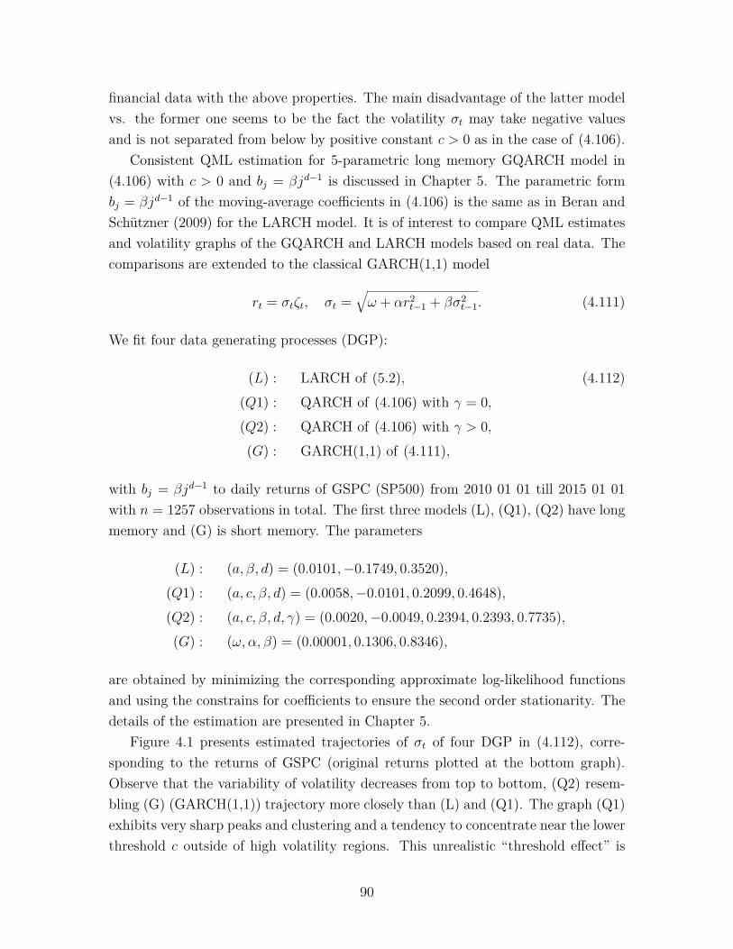
financial data with the above properties. The main disadvantage of the latter modelvs. the former one seems to be the fact the volatility σt may take negative valuesand is not separated from below by positive constant c > 0 as in the case of (4.106).
Consistent QML estimation for 5-parametric long memory GQARCH model in(4.106) with c > 0 and bj = βjd−1 is discussed in Chapter 5. The parametric formbj = βjd−1 of the moving-average coefficients in (4.106) is the same as in Beran andSchützner (2009) for the LARCH model. It is of interest to compare QML estimatesand volatility graphs of the GQARCH and LARCH models based on real data. Thecomparisons are extended to the classical GARCH(1,1) model
rt = σtζt, σt =√ω + αr2
t−1 + βσ2t−1. (4.111)
We fit four data generating processes (DGP):
(L) : LARCH of (5.2), (4.112)(Q1) : QARCH of (4.106) with γ = 0,(Q2) : QARCH of (4.106) with γ > 0,(G) : GARCH(1,1) of (4.111),
with bj = βjd−1 to daily returns of GSPC (SP500) from 2010 01 01 till 2015 01 01with n = 1257 observations in total. The first three models (L), (Q1), (Q2) have longmemory and (G) is short memory. The parameters
(L) : (a, β, d) = (0.0101,−0.1749, 0.3520),(Q1) : (a, c, β, d) = (0.0058,−0.0101, 0.2099, 0.4648),(Q2) : (a, c, β, d, γ) = (0.0020,−0.0049, 0.2394, 0.2393, 0.7735),(G) : (ω, α, β) = (0.00001, 0.1306, 0.8346),
are obtained by minimizing the corresponding approximate log-likelihood functionsand using the constrains for coefficients to ensure the second order stationarity. Thedetails of the estimation are presented in Chapter 5.
Figure 4.1 presents estimated trajectories of σt of four DGP in (4.112), corre-sponding to the returns of GSPC (original returns plotted at the bottom graph).Observe that the variability of volatility decreases from top to bottom, (Q2) resem-bling (G) (GARCH(1,1)) trajectory more closely than (L) and (Q1). The graph (Q1)exhibits very sharp peaks and clustering and a tendency to concentrate near the lowerthreshold c outside of high volatility regions. This unrealistic “threshold effect” is
90
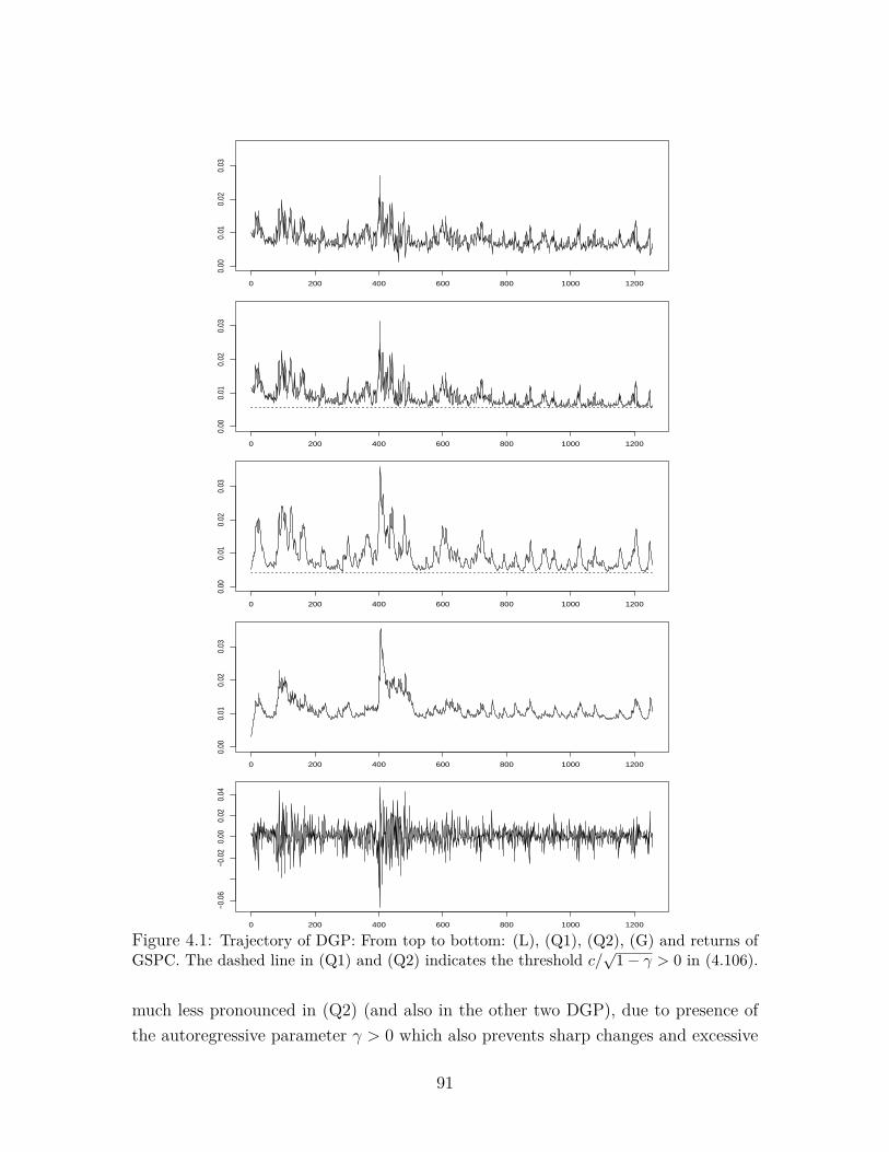
0 200 400 600 800 1000 1200
0.00
0.01
0.02
0.03
0 200 400 600 800 1000 1200
0.00
0.01
0.02
0.03
0 200 400 600 800 1000 1200
0.00
0.01
0.02
0.03
0 200 400 600 800 1000 1200
0.00
0.01
0.02
0.03
0 200 400 600 800 1000 1200
−0.0
6−0
.02
0.00
0.02
0.04
Figure 4.1: Trajectory of DGP: From top to bottom: (L), (Q1), (Q2), (G) and returns ofGSPC. The dashed line in (Q1) and (Q2) indicates the threshold c/
√1− γ > 0 in (4.106).
much less pronounced in (Q2) (and also in the other two DGP), due to presence ofthe autoregressive parameter γ > 0 which also prevents sharp changes and excessive
91
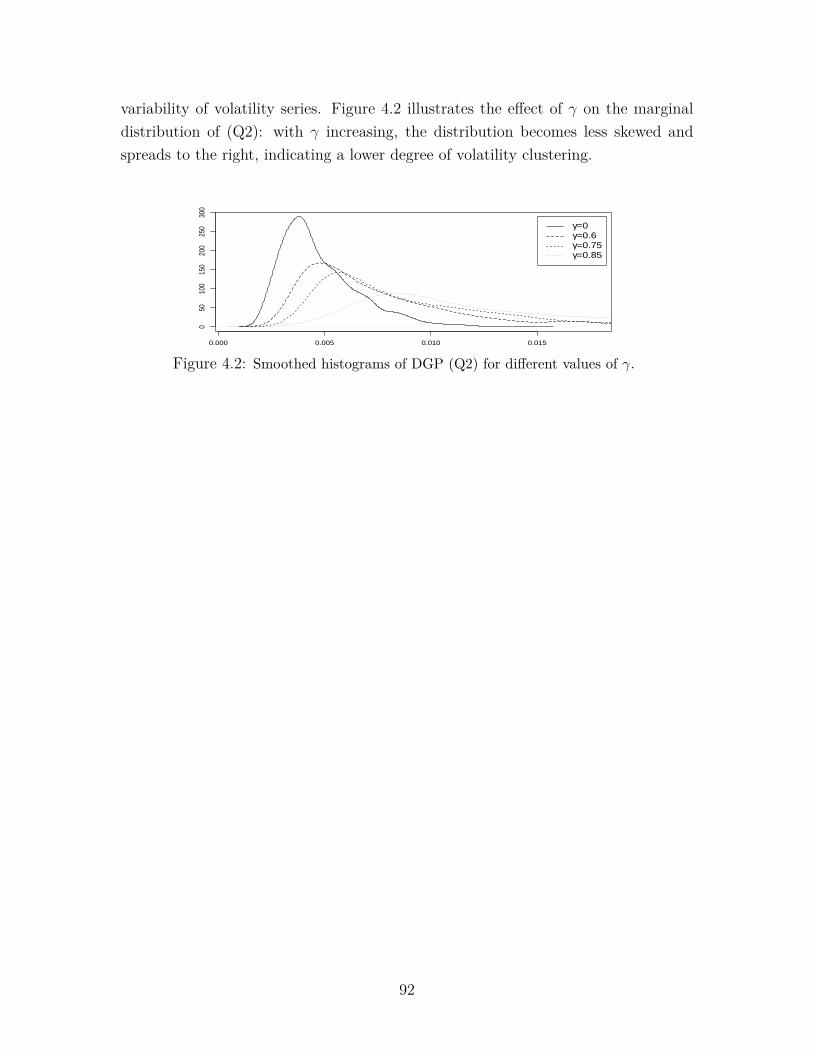
variability of volatility series. Figure 4.2 illustrates the effect of γ on the marginaldistribution of (Q2): with γ increasing, the distribution becomes less skewed andspreads to the right, indicating a lower degree of volatility clustering.
0.000 0.005 0.010 0.015
050
100
150
200
250
300
γ=0γ=0.6γ=0.75γ=0.85
Figure 4.2: Smoothed histograms of DGP (Q2) for different values of γ.
92
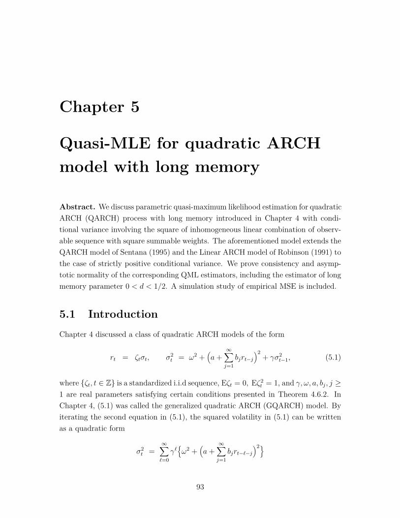
Chapter 5
Quasi-MLE for quadratic ARCHmodel with long memory
Abstract. We discuss parametric quasi-maximum likelihood estimation for quadraticARCH (QARCH) process with long memory introduced in Chapter 4 with condi-tional variance involving the square of inhomogeneous linear combination of observ-able sequence with square summable weights. The aforementioned model extends theQARCH model of Sentana (1995) and the Linear ARCH model of Robinson (1991) tothe case of strictly positive conditional variance. We prove consistency and asymp-totic normality of the corresponding QML estimators, including the estimator of longmemory parameter 0 < d < 1/2. A simulation study of empirical MSE is included.
5.1 Introduction
Chapter 4 discussed a class of quadratic ARCH models of the form
rt = ζtσt, σ2t = ω2 +
(a+
∞∑j=1
bjrt−j)2
+ γσ2t−1, (5.1)
where ζt, t ∈ Z is a standardized i.i.d sequence, Eζt = 0, Eζ2t = 1, and γ, ω, a, bj, j ≥
1 are real parameters satisfying certain conditions presented in Theorem 4.6.2. InChapter 4, (5.1) was called the generalized quadratic ARCH (GQARCH) model. Byiterating the second equation in (5.1), the squared volatility in (5.1) can be writtenas a quadratic form
σ2t =
∞∑`=0
γ`ω2 +
(a+
∞∑j=1
bjrt−`−j)2
93
in lagged variables rt−1, rt−2, . . . , and hence it represents a particular case of QuadraticARCH model by Sentana (1995) with p =∞. The model (5.1) includes the classicalAsymmetric GARCH(1,1) process of Engle (1990) and the Linear ARCH (LARCH)model of Robinson (1991):
rt = ζtσt, σt = a+∞∑j=1
bjrt−j. (5.2)
The main interest in (5.1) and (5.2) seems the possibility of having slowly decayingmoving-average coefficients bj with ∑∞
j=1 |bj| = ∞, ∑∞j=1 b2j < ∞ for modeling long
memory in volatility, in which case rt and ζt must have zero mean in order that theseries ∑∞j=1 bjrt−j converges. Giraitis et al. (2000) proved that the squared stationarysolution r2
t of the LARCH model in (5.2) with bj decaying as jd−1, 0 < d < 1/2 mayhave long memory autocorrelations. For the GQARCH model in (5.1), similar resultswere established in Chapter 4. Namely, assume that the parameters γ, ω, a, bj, j ≥ 1in (5.1) satisfy
bj ∼ c jd−1 (∃ 0 < d < 1/2, c > 0),
γ ∈ [0, 1), a 6= 0 and
6B2 + 4|µ3|∞∑j=1|bj|3 + µ4
∞∑j=1
b4j < (1− γ)2, (5.3)
where µp := Eζp0 , p = 1, 2, . . . , B2 := ∑∞j=1 b
2j . Then (see Chapter 4, Theorems 4.6.2
and 4.6.3) there exists a stationary solution of (5.1) with Er4t <∞ such that
Cov(r20, r
2t ) ∼ κ2
1t2d−1, t→∞
and
n−d−1/2[nτ ]∑t=1
(r2t − Er2
t ) →D[0,1] κ2Wd+(1/2)(τ), n→∞,
whereWd+(1/2) is a fractional Brownian motion with Hurst parameterH = d+(1/2) ∈(1/2, 1) and κi > 0, i = 1, 2 are some constants.
As noted in Chapter 4, the GQARCH model of (5.1) and the LARCH model of(5.2) have similar long memory and leverage properties and both can be used formodelling of financial data with the above properties. The main disadvantage of thelatter model vs. the former one seems to be the fact that volatility σt in (5.2) mayassume negative values and is not separated from below by positive constant c > 0as in the case of (5.1). The standard quasi-maximum likelihood (QML) approach to
94
estimation of LARCH parameters is inconsistent and other estimation methods weredeveloped in Beran and Schützner (2009), Francq and Zakoian (2010b), Levine et al.(2009), Truquet (2014).
The present chapter discusses QML estimation for the 5-parametric GQARCHmodel
σ2t (θ) =
∞∑`=0
γ`ω2 +
(a+ c
∞∑j=1
jd−1rt−`−j)2
, (5.4)
depending on parameter θ = (γ, ω, a, d, c), 0 < γ < 1, ω > 0, a 6= 0, c 6= 0 and d ∈(0, 1/2). The parametric form bj = c jd−1 of moving-average coefficients in (5.4) is thesame as in Beran and Schützner (2009) for the LARCH model. Similarly as in Beranand Schützner (2009) we discuss the QML estimator θn := arg minθ∈Θ Ln(θ), Ln(θ) :=1n
∑nt=1
(r2t
σ2t (θ) + log σ2
t (θ))
involving exact conditional variance in (5.4) depending on
infinite past rs,−∞ < s < t, and its more realistic version θn := arg minθ∈Θ Ln(θ),obtained by replacing the σ2
t (θ)’s in (5.4) by σ2t (θ) depending only rs, 1 ≤ s < t (see
Section 5.2 for the definition). It should be noted that the QML function in Beran andSchützner (2009) is modified to avoid the degeneracy of σ−1
t in (5.2), by introducingan additional tuning parameter ε > 0 which affects the performance of the estimatorand whose choice is a non-trivial task. For the GQARCH model (5.4) with ω > 0the above degeneracy problem does not occur and we deal with unmodified QMLEin contrast to Beran and Schützner (2009). We also note that our proofs use differenttechniques from Beran and Schützner (2009). Particularly, the method of orthogonalVolterra expansions of the LARCH model used in Beran and Schützner (2009) is notapplicable for model (5.4), see Chapter 4, Example 4.2.1.
This chapter is organized as follows. In Section 5.2 we define several QML esti-mators of parameter θ in (5.4). Section 5.3 presents the main results of the paperdevoted to consistency and asymptotic normality of the QML estimators. The proofsin this section are based on four lemmas presented in Section 5.4. Finite sampleperformance of these estimators is investigated in the simulation study in Section5.5.
5.2 QML estimators
Let Ft = σ(ζs, s ≤ t), t ∈ Z be the sigma-field generated by ζs, s ≤ t. For real p ≥ 2,define as in Chapter 4 Section 4.6
Bp :=( ∞∑j=1
b2j
)p/2, Bp,γ := Bp/(1− γ)p/2. (5.5)
95
The following assumptions on the parametric GQARCH model in (5.4) are im-posed.
Assumption (A): ζt is a standardized i.i.d. sequence with Eζt = 0,Eζ2t = 1.
Assumption (B): Θ ⊂ R5 is a compact set of parameters θ = (γ, ω, a, d, c) definedby
(i) γ ∈ [γ1, γ2] with 0 < γ1 < γ2 < 1;
(ii) ω ∈ [ω1, ω2] with 0 < ω1 < ω2 <∞;
(iii) a ∈ [a1, a2] with −∞ < a1 < a2 <∞;
(iv) d ∈ [d1, d2] with 0 < d1 < d2 < 1/2;
(v) c ∈ [c1, c2] with 0 < ci = ci(d, γ) <∞, c1 < c2 such that B2 = c2∑∞j=1 j
2(d−1) <
1− γ for any c ∈ [c1, c2], γ ∈ [γ1, γ2], d ∈ [d1, d2].
We assume that the observations rt, 1 ≤ t ≤ n follow the model in (5.1) with thetrue parameter θ0 = (γ0, ω0, a0, d0, c0) belonging to the interior Θ0 of Θ in Assumption(B). The restriction on parameter c in (v) is due to condition (4.89) in Theorem 4.6.2with p = 2. The QML estimator of θ ∈ Θ is defined as
θn := arg minθ∈Θ
Ln(θ), (5.6)
whereLn(θ) = 1
n
n∑t=1
(r2t
σ2t (θ)
+ log σ2t (θ)
)(5.7)
and σ2t (θ) is defined in (5.4), viz.,
σ2t (θ) =
∞∑`=0
γ`ω2 +
(a+ cYt−`(d)
)2, where (5.8)
Yt(d) :=∞∑j=1
jd−1rt−j.
Note the definitions in (5.6)-(5.8) depend on (unobserved) rs, s ≤ 0 and therefore theestimator in (5.6) is usually referred to as the QMLE given infinite past (Beran andSchützner (2009)). A more realistic version of (5.6) is defined as
θn := arg minθ∈Θ
Ln(θ), (5.9)
96
where
Ln(θ) := 1n
n∑t=1
(r2t
σ2t (θ)
+ log σ2t (θ)
), where (5.10)
σ2t (θ) :=
t−1∑`=0
γ`ω2 +
(a+ cYt−`(d)
)2, Yt(d) :=
t−1∑j=1
jd−1rt−j.
Note all quantities in (5.10) depend only on rs, 1 ≤ t ≤ n, hence (5.9) is called theQMLE given finite past. The QML functions in (5.7) and (5.10) can be written as
Ln(θ) = 1n
n∑t=1
lt(θ) and Ln(θ) = 1n
n∑t=1
lt(θ)
respectively, where
lt(θ) := r2t
σ2t (θ)
+ log σ2t (θ), lt(θ) := r2
t
σ2t (θ)
+ log σ2t (θ). (5.11)
Finally, following Beran and Schützner (2009) we define a truncated version of (5.9)involving the last O(nβ) quasi-likelihoods lt(θ), n− [nβ] < t ≤ n, as follows:
θ(β)n := arg min
θ∈ΘL(β)n (θ), L(β)
n (θ) := 1[nβ]
n∑t=n−[nβ ]+1
lt(θ). (5.12)
where 0 < β < 1 is a “bandwidth parameter”. Note that for any t ∈ Z and θ0 =(γ0, ω0, a0, d0, c0) ∈ Θ, the random functions Yt(d) and Yt(d) in (5.8) and (5.10) areinfinitely differentiable w.r.t. d ∈ (0, 1/2) a.s. Hence using the explicit form ofσ2t (θ) and σ2
t (θ), it follows that σ2t (θ), σ2
t (θ), lt(θ), lt(θ), Ln(θ), Ln(θ), L(β)n (θ) etc. are
all infinitely differentiable w.r.t. θ ∈ Θ0 a.s. We use the notation
L(θ) := ELn(θ) = Elt(θ) (5.13)
and
A(θ) := E[∇T lt(θ)∇lt(θ)
]and B(θ) := E
[∇T∇lt(θ)
], (5.14)
where ∇ = (∂/∂θ1, . . . , ∂/∂θ5) and the superscript T stands for transposed vector.Particularly, A(θ) and B(θ) are 5× 5-matrices. By Lemma 5.4.1, the expectations in(5.14) are well-defined for any θ ∈ Θ under condition Er4
0 <∞. We have
B(θ) = E[σ−4t (θ)∇Tσ2
t (θ)∇σ2t (θ)] and A(θ) = κ4B(θ), (5.15)
97
where κ4 := E(ζ20 − 1)2 > 0.
5.3 Main results
Everywhere in this section rt is a stationary solution of model (5.4) as definedin Definition 4.6.1 and satisfying Assumptions (A) and (B) of the previous sec-tion. As usual, all expectations are taken with respect to the true value θ0 =(γ0, ω0, a0, d0, c0) ∈ Θ0, where Θ0 is the interior of the parameter set Θ ⊂ R5.
The asymptotic results in Theorems 5.3.1 and 5.3.2 are similar to the results ofBeran and Schützner (2009), Theorems 1-4, pertaining to the 3-parametric LARCHmodel in (5.2) with bj = cjd−1, except that Beran and Schützner (2009) deal witha modified QMLE involving a “tuning parameter” ε > 0. As explained in Beranand Schützner (2009), Section 3.2, the convergence rate of ∇Ln(θ0) and θn (basedon nonstationary truncated observable series in (5.10)) is apparently too slow toguarantee asymptotic normality, this fact being a consequence of long memory involatility and the main reason for introducing the estimators θ(β)
n in (5.12). Theorems5.3.1 and 5.3.2 are based on subsequent Lemmas 5.4.1-5.4.4 which describe propertiesof the likelihood processes defined in (5.7), (5.10) and (5.11). As noted in Section5.1, our proofs use different techniques from Beran and Schützner (2009) which relyon explicit Volterra series representation of stationary solution of the LARCH model.
Theorem 5.3.1 (i) Let E|rt|3 < ∞. Then θn in (5.6) is a strongly consistent esti-mator of θ0, i.e.
θna.s.→ θ0.
(ii) Let E|rt|5 <∞. Then θn in (5.6) is asymptotically normal:
n1/2(θn − θ0
)law→ N(0,Σ(θ0)), (5.16)
where Σ(θ0) := B−1(θ0)A(θ0)B−1(θ0) = κ4B−1(θ0) and matrices A(θ), B(θ) are de-
fined in (5.15).
Proof. (i) Follows from Lemmas 5.4.2 and 5.4.4 (i) using standard argument.(ii) By Taylor’s expansion,
0 = ∇Ln(θn) = ∇Ln(θ0) +∇T∇Ln(θ∗n)(θn − θ0),
where θ∗n →p θ0 since θn →p θ0. Then ∇T∇Ln(θ∗n) →p ∇T∇L(θ0) by Lemma 5.4.4(5.57). Next, since r2
t /σ2t (θ0) − 1,Ft, t ∈ Z is a square-integrable and ergodic
98
martingale difference sequence, the convergence n1/2∇Ln(θ0) law→ N(0, A(θ0)) followsby the martingale central limit theorem in (Billingsley (1968), Therem 23.1). Then(5.16) follows by Slutsky’s theorem and (5.14).
The following theorem gives asymptotic properties of “finite past” estimators θnand θ(β)
n defined in (5.9) and (5.12), respectively.
Theorem 5.3.2 (i) Let E|rt|3 <∞ and 0 < β < 1. Then
E|θn − θ0| → 0 and E|θ(β)n − θ0| → 0.
(ii) Let E|rt|5 <∞ and 0 < β < 1− 2d0. Then
nβ/2(θ(β)n − θ0) law→ N(0,Σ(θ0)), (5.17)
where Σ(θ0) is the same as in Theorem 5.3.1.
Proof. Part (i) follows from Lemmas 5.4.2 and 5.4.4 (i) as in the case of Theorem5.3.1 (i).
To prove part (ii), by Taylor’s expansion
0 = ∇L(β)n (θ(β)
n ) = ∇L(β)n (θ0) +∇T∇L(β)
n (θ∗n)(θ(β)n − θ0),
where θ∗n →p θ0 since θ(β)n →p θ0. Then ∇T∇L(β)
n (θ∗n)→p ∇T∇L(θ0) by Lemma 5.4.4(5.57)-(5.58). From the proof of Theorem 5.3.1 (ii) we have that nβ/2∇L(β)
n (θ0) law→N(0, A(θ0)), where L(β)
n (θ) := 1[nβ ]
∑nt=n−[nβ ]+1 lt(θ). Hence, the central limit theorem
in (5.17) follows from
In(β) := E|∇L(β)n (θ0)−∇L(β)
n (θ0)| = o(n−β/2). (5.18)
We have In(β) ≤ supn−[nβ ]≤t≤n E|∇lt(θ0)−∇lt(θ0)| and (5.18) follows from
E|∇lt(θ0)−∇lt(θ0)| = o(t−β/2), t→∞. (5.19)
Write ‖ξ‖p := E1/p|ξ|p for Lp-norm of r.v. ξ. Using |∇(lt(θ0)−lt(θ0))| ≤ r2t |∇(σ−2
t (θ0)−σ−2t (θ0))| + |∇(log σ2
t (θ0) − log σ2t (θ0))| and assumption E|rt|5 < ∞, relation (5.19)
follows from
‖σ−4t ∂iσ
2t − σ−4
t ∂iσ2t ‖5/3 = O(td0−1/2 log t) and (5.20)
‖σ−2t ∂iσ
2t − σ−2
t ∂iσ2t ‖1 = O(td0−1/2 log t), i = 1, . . . , 5,
99
where σ2t := σ2
t (θ0), σ2t := σ2
t (θ0), ∂iσ2t := ∂iσ
2t (θ0), ∂iσ2
t := ∂iσ2t (θ0). Below, we
prove the first relation (5.20) only, the proof of the second one being similar. Wehave σ−4
t ∂iσ2t − σ−4
t ∂iσ2t = σ−4
t σ−4t (σ2
t + σ2t )(σ2
t − σ2t )∂iσ2
t + σ−4t (∂iσ2 − ∂iσ2
t ). Thenusing σ2
t ≥ ω21/(1− γ2) > 0, σ2
t ≥ ω21/(1− γ2) > 0, relation the first relation in (5.20)
follows from
‖(σ2t − σ2
t )(∂iσ2t /σt)‖5/3 = O(td0−1/2) and (5.21)
‖∂iσ2t − ∂iσ2
t ‖5/3 = O(td0−1/2 log t), i = 1, . . . , 5. (5.22)
Consider (5.21). By Hölder’s inequality,
‖(σ2t − σ2
t )(∂iσ2t /σt)‖5/3 ≤ ‖σ2
t − σ2t ‖5/2‖∂iσ2
t /σt‖5,
where ‖∂iσ2t /σt‖5 < C according to (5.32). Hence, (5.21) follows from
‖σ2t − σ2
t ‖5/2 = O(td0−1/2). (5.23)
To show (5.23), similarly as in the proof of (5.43) split σ2t − σ2
t = Ut,1 + Ut,2, whereUt,i := Ut,i(θ0), i = 1, 2 are defined in (4.57), i.e., Ut,1 = ∑t−1
`=1 γ`0
(a0 + c0Yt−`
)2−(
a0 +c0Yt−`)2
, Ut,2 = ∑∞`=t γ
`0
ω2
0 +(a0 +c0Yt−`
)2and Yt := Yt(d0), Yt := Yt(d0). We
have |Ut,1| ≤ C∑t−1`=1 γ
`0|Yt−`− Yt−`|(1+ |Yt−`|+ |Yt−`|), |Ut,2| ≤ C
∑∞`=t γ
`0(1+ |Yt−`|2)
and hence
‖σ2t − σ2
t ‖5/2 ≤ C t−1∑`=1
γ`0‖(Yt−` − Yt−`)(1 + |Yt−`|+ |Yt−`|)‖5/2
+∞∑`=t
γ`0(1 + ‖Yt−`‖5)
≤ C t−1∑`=1
γ`0‖Yt−` − Yt−`‖5 +∞∑`=t
γ`0
, (5.24)
where we used the fact that ‖Yt‖5 < C, ‖Yt‖5 < C by ‖rt‖5 < C and Rosenthal’sinequality in (4.13). In a similar way from (4.13) it follows that
‖Yt−` − Yt−`‖5 ≤ C ∑j>t−`
j2(d0−1)1/2
≤ C(t− `)d0−1/2. (5.25)
Substituting (5.25) into (5.24) we obtain
‖σ2t − σ2
t ‖5/2 ≤ C t−1∑`=1
γ`0(t− `)d0−1/2 +∞∑`=t
γ`0
= O(td0−1/2),
100
proving (5.23).It remains to show (5.22). Similarly as above, ∂iσ2
t − ∂iσ2t = ∂iUt,1 + ∂iUt,2, where
∂iUt,j := ∂iUt,j(θ0), j = 1, 2. Then (5.22) follows from
‖∂iUt,1‖5/3 = O(td0−1/2 log t) and ‖∂iUt,2‖5/3 = o(td0−1/2), i = 1, . . . , 5. (5.26)
For i = 1, the proof of (5.26) is similar to (5.24). Consider (5.26) for 2 ≤ i ≤ 5.Denote Vt(θ) := 2a+ c(Yt(d) + Yt(d)), Vt := Vt(θ0), ∂iVt := ∂iVt(θ0), then
‖∂iUt,1‖5/3 ≤ Ct−1∑`=1
γ`0
‖∂i(Yt−` − Yt−`)‖5‖Vt‖5 + ‖Yt−` − Yt−`‖5‖∂iVt‖5
,
where ∂i(Yt−` − Yt−`) = 0, ∂i 6= ∂d and
‖∂d(Yt − Yt)‖5 = ‖∑j>t
jd0−1(log j)rt−j‖5
≤ C∑j>t
j2(d0−1) log2 j1/2
= O(td0−1/2 log t)
similarly as in (5.25) above. Hence, the first relation in (5.26) follows from (5.25) and‖∂iVt‖5 ≤ C(1 + ‖∂dYt−`‖5 + ‖∂dYt−`‖5) ≤ C <∞ as in the proof of (5.22), and theproof of the second relation in (5.26) is analogous. This proves (5.19) and completesthe proof of Theorem 5.3.2.
Remark 5.3.1 As noted above, the moment conditions of Theorems 5.3.1 and 5.3.2are similar to those in Beran and Schützner (2009) for the LARCH model. Particu-larly, condition (M′5) in Beran and Schützner (2009), Theorems 2 and 5, for asymp-totic normality of estimators ensures E|rt|5 < ∞. This situation is very differentfrom GARCH models where strong consistency and asymptotic normality of QMLestimators holds under virtually no moment assumption on the observed process (seee.g. Francq and Zakoian (2010a), Chapter 7). The main reason for this differenceseems to be the fact that differentiation with respect to d of Yt(d) = ∑∞
j=1 jd−1rt−j
in (5.8) affects all terms of this series and results in “new” long memory processes∂iYt(d)/∂di = ∑∞
j=1 jd−1(log j)irt−j, i = 1, 2, 3 which are not bounded by C|Yt(d)|
or Cσ2t (θ). Therefore, derivatives of σ−2
t (θ) in (5.8) are much more difficult to con-trol than in the GARCH case, where these quantities are bounded (see Francq andZakoian (2010a), proof of Theorem 7.2).
Remark 5.3.2 We expect that our results can be extended to more general para-
101
metric coefficients, e.g. fractional filters bj(c, d), j ≥ 1 with transfer function
∞∑j=1
e−ijxbj(c, d) = g(c, d)((1− eix)−d − 1), x ∈ [−π, π],
where g(c, d) is a smooth function of (c, d) ∈ (0,∞)× (0, 1/2). Particularly,
bj(c, d) := g(c, d) Γ(j + d)Γ(d)Γ(j + 1) ∼
g(c, d)Γ(d) j
d−1, j →∞ (5.27)
and ∑∞j=1 b2j(c, d) = g2(c, d)(Γ(1− 2d)− Γ2(1− d))/Γ2(1− d), see e.g. Giraitis et al.
(2012), Chapter 7. See also Beran and Schützner (2009), Section 2.2. The impor-tant condition used in our proofs and satisfied by bj(c, d) in (5.27) is that the partialderivatives ∂idbj(c, d), i = 1, 2, 3 decay at a similar rate jd−1 (modulus a slowly varyingfactor). Particularly, for ARFIMA(0, d, 0) coefficients b0
j(d) := Γ(j + d)/Γ(d)Γ(j +1) = ∏j
k=1d+k−1k
it easily follows that ∂db0j(d) = b0
j(d)∑jk=1
1d+k−1 ∼ b0
j(d) log j ∼Γ(d)−1jd−1 log j and, similarly, ∂idb0
j(d) ∼ b0j(d)(log j)i ∼ Γ(d)−1jd−1(log j)i, j →
∞, i = 2, 3.
5.4 Lemmas
For multi-index i = (i1, . . . , i5) ∈ N5, i 6= 0 = (0, . . . , 0), |i| := i1 + · · · + i5, denotepartial derivative ∂i := ∂|i|/
∏5j=1 ∂
ijθij .
Lemma 5.4.1 Let E|rt|2+p <∞, for some integer p ≥ 1. Then for any i ∈ N5, 0 <|i| ≤ p,
E supθ∈Θ|∂ilt(θ)| <∞. (5.28)
Moreover, if E|rt|2+p+ε <∞ for some ε > 0 and p ∈ N then for any i ∈ N5, 0 ≤ |i| ≤p
E supθ∈Θ|∂i(lt(θ)− lt(θ))| → 0, t→∞. (5.29)
102
Proof. We use the following (Faa di Bruno) differentiation rule:
∂iσ−2t (θ) =
|i|∑ν=1
(−1)νν!σ−2(1+ν)t (θ)
∑j1+···+jν=i
χj1,...,jν
ν∏k=1
∂jkσ2t (θ), (5.30)
∂i log σ2t (θ) =
|i|∑ν=1
(−1)ν−1(ν − 1)!σ−2νt (θ)
∑j1+···+jν=i
χj1,...,jν
ν∏k=1
∂jkσ2t (θ),
where the sum ∑j1+···+jν=i is taken over decompositions of i into a sum of ν multi-
indices jk 6= 0, k = 1, . . . , ν, and χj1,...,jνis a combinatorial factor depending only
on jk, 1 ≤ k ≤ ν.Let us prove (5.28). We have |∂ilt(θ)| ≤ r2
t |∂iσ−2t (θ)|+ |∂i log σ2
t (θ)|. Hence using(5.30) and the fact that σ2
t (θ) ≥ ω2/(1− γ) ≥ ω21/(1− γ2) > 0 we obtain
supθ∈Θ|∂ilt(θ)| ≤ C(r2
t + 1)|i|∑ν=1
∑j1+···+jν=i
ν∏k=1
supθ∈Θ
(|∂jkσ2t (θ)|/σt(θ)).
Therefore by Hölder’s inequality
E supθ∈Θ|∂ilt(θ)| ≤ C(E(r2
t + 1)(2+p)/2)2/(2+p)
×|i|∑ν=1
∑j1+···+jν=i
ν∏k=1
E1/qk(
supθ∈Θ|∂jkσ2
t (θ)|/σt(θ))qk, (5.31)
where ∑νj=1 1/qj ≤ p/(2 + p). Note |i| = ∑ν
k=1 |jk| and hence the choice qk =(2 + p)/|jk| satisfies ∑ν
j=1 1/qj = ∑νk=1 |jk|/(2 + p) ≤ p/(2 + p). Using (5.31) and
condition E|rt|2+p ≤ C, relation (5.28) follows from
E supθ∈Θ
(|∂jσ2
t (θ)|/σt(θ))(2+p)/|j |
< ∞ (5.32)
for any multi-index j ∈ N5, 1 ≤ |j| ≤ p.Consider first the case |j| = 1, or the partial derivative ∂iσ2
t (θ) = ∂σ2t (θ)/∂θi, 1 ≤
103
i ≤ 5. We have
∂iσ2t (θ) =
∑∞`=1 `γ
`−1ω2 +
(a+ cYt−`(d)
)2, θi = γ,∑∞
`=0 γ`2ω, θi = ω,∑∞
`=0 γ`2(a+ cYt−`(d)
), θi = a,∑∞
`=0 γ`2(a+ cYt−`(d)
)Yt−`(d), θi = c,∑∞
`=0 γ`2c(a+ cYt−`(d)
)∂dYt−`(d), θi = d.
(5.33)
We claim that there exist C > 0, 0 < γ < 1 such that
supθ∈Θ
∣∣∣∂iσ2t (θ)
σt(θ)∣∣∣ ≤ C(1 + Jt,0 + Jt,1), i = 1, . . . , 5, where (5.34)
Jt,0 :=∞∑`=0
γ` supd∈[d1,d2]
|Yt−`(d)|, Jt,1 :=∞∑`=0
γ` supd∈[d1,d2]
|∂dYt−`(d)|.
Consider (5.34) for θi = γ. Using `2γ`−2 ≤ Cγ` for all ` ≥ 1, γ ∈ [γ1, γ2] ⊂ (0, 1)and some C > 0, 0 < γ < 1 together with Assumption (B) and Cauchy inequality,we obtain |∂γσ2
t (θ)|/σt(θ) ≤(∑∞
`=1 `2γ`−2
ω2 +
(a + cYt−`(d)
)2)1/2≤ C(1 + Jt,0)
uniformly in θ ∈ Θ, proving (5.34) for θi = γ. Similarly, |∂cσ2t (θ)|/σt(θ) ≤ C(1 +Jt,0)
and |∂dσ2t (θ)|/σt(θ) ≤ C(1 + Jt,1). Finally, for θi = ω and θi = a, (5.34) is immediate
from (5.33), proving (5.34).With (5.34) in mind, (5.32) for |j| = 1 follows from
EJ2+pt,i = E
( ∞∑`=0
γ` supd∈[d1,d2]
|∂idYt−`(d)|)2+p
< ∞, i = 0, 1. (5.35)
Using Minkowski’s inequality and stationarity of Yt(d) we obtain E1/(2+p)J2+pt,i ≤∑∞
`=0 γ` E1/(2+p) supd |∂idYt−`(d)|2+p ≤ C(E supd |∂idYt(d)|2+p)1/(2+p), where ∂idYt(d) =∑∞
j=1 ∂idjd−1rt−j. Hence using Beran and Schützner (2009), Lemma 1 (b) and the
inequality xy ≤ xq/q + yq′/q′, x, y > 0, 1/q + 1/q′ = 1 we obtain
1∑i=0
EJ2+pt,i ≤ C
1∑i=0
E supd∈[d1,d2]
|∂idYt(d)|2+p
≤ C2∑i=0
supd∈[d1,d2]
E|∂idYt(d)|2+p < ∞ (5.36)
104
since
supd∈[d1,d2]
E|∂idYt(d)|2+p ≤ C supd∈[d1,d2]
( ∞∑j=1
(∂idjd−1)2(E|rt−j|2+p)2/(2+p))(2+p)/2
<∞
according to condition E|rt|2+p < C, Rosenthal’s inequality in (4.13) and the factthat supd∈[d1,d2]
∑∞j=1(∂idjd−1)2 ≤ supd∈[d1,d2]
∑∞j=1 j
2(d−1)(1 + log2 j)2 < C, i = 0, 1, 2.This proves (5.32) for |j| = 1.
The proof of (5.32) for 2 ≤ |j| ≤ p is simpler since it reduces to
E supθ∈Θ|∂jσ2
t (θ)|(p+2)/2 < ∞, 2 ≤ |j| ≤ p. (5.37)
Recall θ1 = γ and j ′ := j − (j1, 0, 0, 0, 0) = (0, j2, j3, j4, j5). If j ′ = 0 thensupθ∈Θ |∂jσ2
t (θ)| ≤ CJt,0 follows as in (5.34) implying (5.37) as in (5.36) above.Next, let j ′ 6= 0. Denote
Q2t (θ) := ω2 +
(a+ cYt(d)
)2(5.38)
so that σ2t (θ) = ∑∞
`=0 γ`Q2
t−`(θ). We have with m := j1 ≥ 0 that |∂jσ2t (θ)| ≤∑∞
`=m(`!/(`−m)!)γ`−m |∂j ′Q2t−`(θ)| and (5.32) follows from
E supθ∈Θ|∂jQ2
t (θ)|(p+2)/2 < ∞. (5.39)
For j2 6= 0 (recall θ2 = ω) the derivative in (5.39) is trivial so that it suffices to check(5.39) for j1 = 0 only. Then applying Faa di Bruno’s rule we get
|∂jQ2t (θ)|(p+2)/2 ≤ C
∑j1+j2=j
|∂j1(a+ cYt(d))|(p+2)/2|∂j2(a+ cYt(d))|(p+2)/2
and hence (5.39) reduces to
E supθ∈Θ|∂j(a+ cYt(d))|p+2 < ∞, 0 ≤ |j| ≤ p,
whose proof is similar to (5.35) above. This ends the proof of (5.28).The proof of (5.29) is similar. We have |∂i(lt(θ) − lt(θ))| ≤ r2
t |∂i(σ−2t (θ) −
σ−2t (θ))|+ |∂i(log σ2
t (θ)− log σ2t (θ))|. Hence, using Hölder’s inequality similarly as in
105
the proof of (5.28) it suffices to show
E supθ∈Θ|∂i(σ−2
t (θ)− σ−2t (θ))|
p+2p → 0 and
E supθ∈Θ|∂i(log σ2
t (θ)− log σ2t (θ))|
p+2p → 0. (5.40)
Below, we prove the first relation in (5.40) only, the proof of the second one beinganalogous.
Using the differentiation rule in (5.30) we have that
|∂i(σ−2t (θ)− σ−2
t (θ))| ≤ C|i|∑ν=1
∑j1+···+jν=i
∣∣∣Wj1,...,jνt (θ)− Wj1,...,jν
t (θ)∣∣∣,
where
Wj1,...,jνt (θ) := σ
−2(1+ν)t (θ)∏ν
k=1 ∂jkσ2
t (θ),
Wj1,...,jνt (θ) := σ
−2(1+ν)t (θ)∏ν
k=1 ∂jk σ2
t (θ).
Whence, (5.40) follows from
supθ∈Θ|Wj1,...,jν
t (θ)− Wj1,...,jνt (θ)| →p 0, t→∞ (5.41)
andE supθ∈Θ
(|Wj1,...,jν
t (θ)|+ |Wj1,...,jνt (θ)|
)(p+2+ε)/p≤ C <∞ (5.42)
for some constants ε > 0 and C > 0 independent of t. In turn, (5.41) and (5.42)follow from
supθ∈Θ|∂j(σ2
t (θ)− σ2t (θ))| →p 0, t→∞ (5.43)
and
E supθ∈Θ
(|∂jσ2
t (θ)|/σt(θ))(2+p+ε)/|j |
< C, (5.44)
E supθ∈Θ
(|∂j σ2
t (θ)|/σt(θ))(2+p+ε)/|j |
< C,
for any multi-index j such that |j| ≥ 0 and 1 ≤ |j| ≤ p, respectively.Using condition E|rt|2+p+ε < C, relations in (5.44) can be proved analogously to
(5.32) and we omit the details. Consider (5.43). Split σ2t (θ)−σ2
t (θ) = Ut,1(θ)+Ut,2(θ),
106
where
Ut,1(θ) :=t−1∑`=1
γ`(a+ cYt−`(d)
)2−(a+ cYt−`(d)
)2, (5.45)
Ut,2(θ) :=∞∑`=t
γ`ω2 +
(a+ cYt−`(d)
)2.
Then supθ∈Θ |∂jUt,i(θ)| →p 0, t→∞, i = 1, 2 follows by using Assumption (B) andconsidering the bounds on the derivatives as in the proof of (5.32). For instance,let us prove (5.43) for ∂j = ∂d, |j| = 1. We have |∂dUt,1(θ)| ≤ C
∑t−1`=1 γ
`
(1 +|Yt−`(d)|)|∂d(Yt−`(d) − Yt−`(d))| + |∂dYt−`(d)| |Yt−`(d) − Yt−`(d)|
.
Hence, supθ∈Θ |∂dUt,1(θ)| →p 0 follows from 0 ≤ γ ≤ γ2 < 1 and
E supd∈[d1,d2]
(|Yt(d)− Yt(d)|2 + |∂d(Yt(d)− Yt(d))|2) → 0 and (5.46)
E supd∈[d1,d2]
(|Yt(d)|2 + |Yt(d)|2 + |∂dYt(d)|2 + |∂dYt(d)|2) ≤ C. (5.47)
The proof of (5.47) mimics that of (5.36) and therefore is omitted. To show (5.46),note Yt(d) − Yt(d) = ∑∞
j=t jd−1rt−j and use a similar argument as in (5.36) to show
that the l.h.s. of (5.47) does not exceed C supd∈[d1,d2]∑2i=0 E|∂id(Yt(d) − Yt(d))|2 ≤
C supd∈[d1,d2]∑∞j=t j
2(d−1) (1 + log2 j) → 0, t → ∞. This proves (5.43) for |j| = 1and ∂j = ∂d. The remaining cases in (5.43) follow similarly and we omit the details.This proves (5.29) and completes the proof of Lemma 5.4.1.
Lemma 5.4.2 The function L(θ), θ ∈ Θ in (5.13) is bounded and continuous. More-over, it attains its unique minimum at θ = θ0.
Proof. We have |L(θ1) − L(θ2)| ≤ E|lt(θ1) − lt(θ2)| ≤ CE|σ2t (θ1) − σ2
t (θ2)|, wherethe last expectation can be easily shown to vanish as |θ1 − θ2| → 0, θ1, θ2 ∈ Θ. Thisproves the first statement of the lemma. To show the second statement of the lemma,write
L(θ)− L(θ0) = E[σ2
t (θ0)σ2t (θ)
− log σ2t (θ0)σ2t (θ)
− 1].
The function f(x) := x − 1 − log x > 0 for x > 0, x 6= 1 and f(x) = 0 if and only ifx = 1. Therefore L(θ) ≥ L(θ0),∀ θ ∈ Θ while L(θ) = L(θ0) is equivalent to
σ2t (θ) = σ2
t (θ0) (Pθ0 − a.s.) (5.48)
Thus, it remains to show that (5.48) implies θ = θ0 = (γ0, ω0, a0, d0, c0). Consider the“projection” Psξ = E[ξ|Fs]− E[ξ|Fs−1] of r.v. ξ, E|ξ| <∞, where Fs = σ(ζu, u ≤ s)
107
(see Section 5.2). (5.48) implies
0 = Ps(σ2t (θ)−σ2
t (θ0)) = Ps(Q2t (θ)−Q2
t (θ0))+(γ−γ0)Psσ2t−1(θ0), ∀ s ≤ t−1, (5.49)
where Q2t (θ) = ω2 +
(a+∑
u<t bt−u(θ)ru)2
is the same as in (5.38). We have
PsQ2t (θ) = 2abt−s(θ)rs + 2bt−s(θ)rs
∑u<s
bt−u(θ)ru +∑s≤u<t
b2t−u(θ)Psr2
u (5.50)
= 2abt−s(θ)ζsσs(θ0) + 2bt−s(θ)ζsσs(θ0)∑u<s
bt−u(θ)ru
+∑s<u<t
b2t−u(θ)Psσ2
u(θ0) + b2t−s(θ)(ζ2
s − 1)σ2s(θ0).
Whence and from (5.49) for s = t− 1 using Pt−1σ2t−1(θ0) = 0 we obtain
C1(θ, θ0)ζ2t−1 + 2C2(θ, θ0)ζt−1 − C1(θ, θ0) = 0 (5.51)
where
C1(θ, θ0) := (c2 − c20)σt−1(θ0),
C2(θ, θ0) := (ac− a0c0) +∑u<t−1
(c2(t− u)d−1 − c20(t− u)d0−1)ru.
Since Ci(θ, θ0), i = 1, 2 are Ft−2-measurable, (5.51) implies C1(θ, θ0) = C2(θ, θ0) = 0,particularly, c = c0 since σt−1(θ0) ≥ ω > 0. Then 0 = C2(θ, θ0) = c0(a − a0) +c2
0∑u<t−1((t − u)d−1 − (t − u)d0−1)ru and Eru = 0 lead to a = a0 and next to 0 =
E(∑u<t−1((t − u)d−1 − (t − u)d0−1)ru)2 = Er20∑j≥2(jd−1 − jd0−1)2 = 0, or d = d0.
Consequently, Ps(Q2t (θ)−Q2
t (θ0)) = 0 for any s ≤ t− 1 and hence γ = γ0 in view of(5.49). Finally, ω = ω0 follows from Eσ2
t (θ) = Eσ2t (θ0) and the fact that ω > 0, ω0 > 0.
This proves θ = θ0 and the lemma, too.
Lemma 5.4.3 Let Er40 <∞. Then matrices A(θ) and B(θ) in (5.14) are well-defined
and strictly positive definite for any θ ∈ Θ.
Proof. From (5.15), it suffices to show that
∇σ2t (θ)λT = 0 (5.52)
for some θ ∈ Θ and λ ∈ R5, λ 6= 0 leads to a contradiction. To the last end, weuse a similar projection argument as in the proof of Lemma 5.4.2. First, note that
108
σ2t (θ) = Q2
t (θ) + γσ2t−1(θ) implies
∇σ2t (θ) = (0,∇4Q
2t (θ)) + γ∇σ2
t−1(θ) + (∇γ)σ2t−1(θ),
where ∇4 = (∂/θ2, . . . , ∂θ5). Hence and using the fact that (5.52) holds for any t ∈ Zby stationarity, from (5.52) we obtain
(σ2t−1(θ),∇4Q
2t (θ))λT = 0. (5.53)
Thus,(Psσ2
t−1(θ), Ps∇T4Q
2t (θ))λ = 0, ∀ s ≤ t− 1;
c.f. (5.49). For s = t − 1 using Pt−1σ2t−1(θ) = 0, Pt−1∇4Q
2t (θ) = ∇4Pt−1Q
2t (θ) by
differentiating (5.50) similarly to (5.51) we obtain
D1(λ)ζ2t−1 + 2D2(λ)ζt−1 −D1(λ) = 0 (5.54)
where D1(λ) := 2λ5σt−1(θ) and
D2(λ) := λ3c+ λ5a+ 2λ5c∑u<t−1
(t− u)d−1ru + λ4c2 ∑u<t−1
(t− u)d−2 log(t− u)ru,
λ = (λ1, . . . , λ5)T . As in (5.51), Di(λ), i = 1, 2 are Ft−2-measurable, (5.54) im-plying Di(λ) = 0, i = 1, 2. Hence, λ5 = 0 and then D2(λ) = 0 reduces to λ3c +λ4c
2∑u<t−1(t − u)d−2 log(t − u)ru = 0. By taking expectation and using c 6= 0 we
get λ3 = 0 and then λ4 = 0 since E(∑u<t−1(t − u)d−2 log(t − u)ru)2 6= 0. The abovefacts allow to rewrite (5.53) as 2ωλ2 + λ1σ
2t−1(θ) = 0. Unless both λ1, λ2 vanish, the
last equation means that either λ1 6= 0 and σ2t (θ) is a deterministic process which
contradicts c 6= 0, or λ1 = 0, λ2 6= 0 and ω = 0, which contradicts ω 6= 0. Lemma5.4.3 is proved.
Write | · | for the Euclidean norm in R5 and in R5 ⊗ R5 (the matrix norm).
Lemma 5.4.4 (i) Let E|rt|3 <∞. Then
supθ∈Θ|Ln(θ)− L(θ)| a.s.→ 0 and E sup
θ∈Θ|Ln(θ)− Ln(θ)| → 0. (5.55)
(ii) Let Er4t <∞. Then ∇L(θ) = E∇lt(θ) and
supθ∈Θ|∇Ln(θ)−∇L(θ)| a.s.→ 0 and E sup
θ∈Θ|∇Ln(θ)−∇Ln(θ)| → 0. (5.56)
109
(iii) Let E|rt|5 <∞. Then ∇T∇L(θ) = E∇T∇`t(θ) = B(θ) (see (5.14)) and
supθ∈Θ |∇T∇Ln(θ)−∇T∇L(θ)| a.s.→ 0, (5.57)E supθ∈Θ |∇T∇Ln(θ)−∇T∇Ln(θ)| → 0. (5.58)
Proof. Consider the first relation in (5.55). The pointwise convergence Ln(θ) a.s.→L(θ) follows by ergodicity of lt(θ) and the uniform convergence in (5.55) fromE supθ∈Θ |∇lt(θ)| <∞, c.f. Beran and Schützner (2009), proof of Lemma 3, which inturn follows from of Lemma 5.4.1 (5.28) with p = 1. The proof of the second relationin (5.55) is immediate from Lemma 5.4.1 (5.29) with p = 0, ε = 1. The proof of thestatements (ii) and (iii) using Lemma 5.4.1 is similar and is omitted.
5.5 Simulation study
In this section we present a short simulation study of the performance of the QMLEfor the GQARCH model in (5.4). The GQARCH model in (5.4) with i.i.d. standardnormal innovations ζt was simulated for −m + 1 ≤ t ≤ m and two sample sizesm = 1000 and m = 5000, using the recurrent formula in (5.1) with zero initialcondition σ−m = 0. The numerical optimization procedure minimized the QMLfunction:
Lm = 1m
m∑t=1
(r2t
σ2t
+ log σ2t
), (5.59)
with
rt = ζtσt, σ2t = ω2 +
(a+ c
t+m−1∑j=1
jd−1rt−j)2
+ γσ2t−1, t = 1, . . . ,m. (5.60)
The QML function in (5.59) can be viewed as a “realistic proxy” to the QMLfunction Ln(θ) in (5.12) with m = nβ since (5.59)-(5.60) similarly to (5.12) use“auxiliary” observations in addition to r1, . . . , rm for computation of m likelihoodsin (5.59). However, the number of “auxiliary” observations in (5.59) equals m anddoes not grow as m1/β = n, 0 < β < 1 − 2d < 1 in the case of (5.60) and Theorem5.3.2 (ii), which is completely unrealistic. Despite of the violation of the conditionm = nβ of Theorem 5.3.2 (ii) in our simulation study, the differences between thesample RMSEs and the theoretical standard deviations are not vital (and sometimeseven insignificant), see Table 5.1 below.
Finite-sample performance of the QML estimator θm minimizing (5.59) was stud-ied for fixed values of parameters γ0 = 0.7, a0 = −0.2, c0 = 0.2 and different values
110
of ω0 = 0.1, 0.01 and the long memory parameter d0 = 0.1, 0.2, 0.3, 0.4. The abovechoice of θ0 = (γ0, ω0, a0, d0, c0) can be explained by the observation that the QMLestimation of γ0, a0, c0 appears to be more accurate and stable in comparison withestimation of ω0 and d0. The small values of ω0 in our experiment reflect the factthat in most real data studied by us, the estimated QML value of ω0 was less than0.05.
The numerical QML minimization was performed under the following constraints:
0.005 ≤ γ ≤ 0.989, 0 ≤ ω ≤ 2, −2 ≤ a ≤ 2, 0 ≤ d ≤ 0.5,
and the value of c in optimization procedure is chosen in a way to guarantee Assump-tion (B) (v) with appropriate 0 < ci(d, γ), i = 1, 2.
The results of the simulation experiment are presented in Table 5.1 below, whichshows the sample R(oot)MSEs of the QML estimates θm = (γm, ωm, am, dm, cm) with100 independent replications, for two sample lengths m = 1000 and m = 5000 andthe above choices of θ0 = (γ0, ω0, a0, d0, c0). The sample RMSEs in Table 5.1 areconfronted with standard deviations (in brackets) of the infinite past estimator in(5.6) computed according to Theorem 5.3.1 (ii) with Σ(θ0) obtained by inverting asimulated matrix B(θ0)/κ4.
A general impression from Table 5.1 is that theoretical standard deviations (brack-eted entries) are generally smaller than the sample RMSEs, however, these differ-ences become less pronounced with increase of m and in some cases (e.g., whenω0 = 0.1,m = 5000) they seem to be insignificant. Some tendencies in Table 5.1are quite surprising, particularly, the decrease of the theoretical standard deviationsand most of sample RMSEs as d0 increases. Also note a sharp increase of theoreticalstandard deviations of ωn when ω0 = 0.01, which can be explained by the fact thatthe derivative ∂ωσ2
t (θ0) = 2ω0/(1 − γ0) becomes very small with ω0, resulting in asmall entry of B(θ0) and a large entry of Σ(θ0). On the other hand, the RMSEsin Table 5.1 appear to be more stable and less dependent on θ0 compared to thebracketed entries (particularly, this applies to errors of ωm and dm).
111
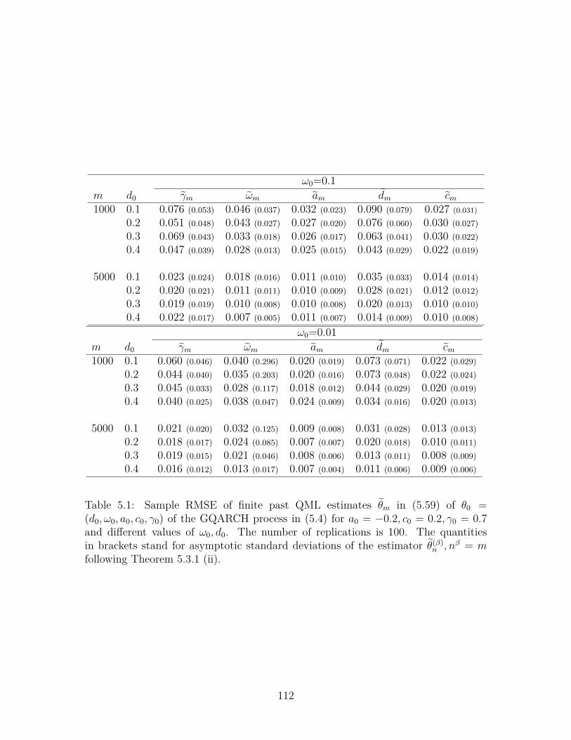
ω0=0.1m d0 γm ωm am dm cm1000 0.1 0.076 (0.053) 0.046 (0.037) 0.032 (0.023) 0.090 (0.079) 0.027 (0.031)
0.2 0.051 (0.048) 0.043 (0.027) 0.027 (0.020) 0.076 (0.060) 0.030 (0.027)0.3 0.069 (0.043) 0.033 (0.018) 0.026 (0.017) 0.063 (0.041) 0.030 (0.022)0.4 0.047 (0.039) 0.028 (0.013) 0.025 (0.015) 0.043 (0.029) 0.022 (0.019)
5000 0.1 0.023 (0.024) 0.018 (0.016) 0.011 (0.010) 0.035 (0.033) 0.014 (0.014)0.2 0.020 (0.021) 0.011 (0.011) 0.010 (0.009) 0.028 (0.021) 0.012 (0.012)0.3 0.019 (0.019) 0.010 (0.008) 0.010 (0.008) 0.020 (0.013) 0.010 (0.010)0.4 0.022 (0.017) 0.007 (0.005) 0.011 (0.007) 0.014 (0.009) 0.010 (0.008)
ω0=0.01m d0 γm ωm am dm cm1000 0.1 0.060 (0.046) 0.040 (0.296) 0.020 (0.019) 0.073 (0.071) 0.022 (0.029)
0.2 0.044 (0.040) 0.035 (0.203) 0.020 (0.016) 0.073 (0.048) 0.022 (0.024)0.3 0.045 (0.033) 0.028 (0.117) 0.018 (0.012) 0.044 (0.029) 0.020 (0.019)0.4 0.040 (0.025) 0.038 (0.047) 0.024 (0.009) 0.034 (0.016) 0.020 (0.013)
5000 0.1 0.021 (0.020) 0.032 (0.125) 0.009 (0.008) 0.031 (0.028) 0.013 (0.013)0.2 0.018 (0.017) 0.024 (0.085) 0.007 (0.007) 0.020 (0.018) 0.010 (0.011)0.3 0.019 (0.015) 0.021 (0.046) 0.008 (0.006) 0.013 (0.011) 0.008 (0.009)0.4 0.016 (0.012) 0.013 (0.017) 0.007 (0.004) 0.011 (0.006) 0.009 (0.006)
Table 5.1: Sample RMSE of finite past QML estimates θm in (5.59) of θ0 =(d0, ω0, a0, c0, γ0) of the GQARCH process in (5.4) for a0 = −0.2, c0 = 0.2, γ0 = 0.7and different values of ω0, d0. The number of replications is 100. The quantitiesin brackets stand for asymptotic standard deviations of the estimator θ(β)
n , nβ = mfollowing Theorem 5.3.1 (ii).
112
Conclusions
The principal goal of this thesis was to introduce new nonlinear models with longmemory which can be used for modelling of financial returns and statistical inference.Apart from long memory, these models are capable to exhibit other stylized factssuch as asymmetry and leverage. The processes studied in the thesis are defined asstationary solutions of certain nonlinear stochastic difference equations involving agiven i.i.d. “noise”. Apart from solvability issues of these equations which are nottrivial by itself, we proved that their solutions exhibit long memory properties asin (1.5) and (1.9). Finally, for a particularly tractable nonlinear parametric modelwith long memory (GQARCH) we prove consistency and asymptotic normality ofquasi-ML estimators.
113
Appendix A
Lemmas
The proofs of Proposition 4.3.1 and Theorems 4.4.2, 4.6.3 use the following lemmas.
Lemma A.1 For αj ≥ 0, j = 1, 2, . . . , denote
Ak := αk +∑
0<p<k
∑0<i1<···<ip<k
αi1αi2−i1 . . . αip−ip−1αk−ip , k = 1, 2, . . . . (A.1)
Assume that A := ∑∞j=1 αj < 1 and
αj ≤ c j−γ (∃ c > 0, γ > 1). (A.2)
Then there exists C > 0 such that for any k ≥ 1
Ak ≤ Ck−γ. (A.3)
Proof. We have Ak = ∑0≤p<k Ak,p, where
Ak,p :=∑
0<i1<···<ip<kαi1αi2−i1 . . . αip−ip−1αk−ip (p ≥ 1), Ak,0 := αk
is the inner sum in (A.1). W.l.g., assume c ≥ 1 in (A.2). Let us prove that thereexists λ > 0 such that
Ak,p ≤ c(p+ 2)λAp+1k−γ, ∀ 0 ≤ p < k <∞. (A.4)
Since A < 1, so (A.4) and ∑p>0(p+ 2)λAp+1 <∞ together imply (A.3).By dividing both sides of (A.4) by Ap+1, it suffices to show (A.4) for A = 1. The
proof uses induction on p. Clearly, (A.4) holds for p = 0. To prove the induction
114
step p− 1→ p ≥ 1, note
Ak,p =∑
0<i<kαiAk−i,p−1 =
∑kp+1<i<k
αiAk−i,p−1 +∑
k− kp+1≤k−i<k
αiAk−i,p−1. (A.5)
Here, αi1(i > kp+1) ≤ ci−γ1(i > k
p+1) ≤ c(p + 1)γk−γ and, similarly, by the inductiveassumption
Ak−i,p−11(k − i ≥ k − k
p+ 1) ≤ c(p+ 1)λ(k − k
p+ 1)−γ = c(p+ 1)λ(p+ 1
p
)γk−γ.
Assumption A = 1 implies ∑k>0Ak,p = 1 for any p ≥ 0. Using the above facts from(A.5) we obtain
Ak,p = c(p+ 1)γkγ
∑k/(p+1)<i<k
Ak−i,p−1 + c(p+ 1)λkγ
(p+ 1p
)γ ∑k−k/(p+1)≤k−i<k
αi
≤ c((p+ 1)γ + (p+ 1)λ
(p+ 1p
)γ)k−γ.
Hence the proof of the induction step p − 1 → p ≥ 1 amounts to verifying theinequality (p+ 1)γ + (p+ 1)λ
(p+1p
)γ≤ (p+ 2)λ, or
nγ + nλ( n
n− 1)γ≤ (n+ 1)λ, n = 2, 3, . . . . (A.6)
The above inequality holds with λ = 3γ. Indeed,
nγ + nλ( n
n− 1)γ
= nλ(n−2γ +( n
n− 1)γ
) ≤ nλ(n−2 +( n
n− 1))γ
≤ nλ(1 + 1n− 1 + 1
n2 )γ ≤ nλ(1 + 3n
+ 3n2 + 1
n3 )γ = (n+ 1)λ,
proving (A.6) and the lemma, too.
Lemma A.2 Assume that 0 ≤ β < 1 and αj ∼ cj−γ (∃ γ > 0, c > 0). Then
αt,β :=t−1∑j=0
βjαt−j ∼c
1− β t−γ, t→∞.
Proof. It suffices to show that the difference Dt := αt,β − αt/(1 − β) decays fasterthan αt, in other words, that
Dt =t−1∑j=0
βj(αt − αt−j)−∞∑j=t
βjαt−j = o(t−γ).
115
Clearly, ∑t/2<j<t βj(αt − αt−j) = O(βt/2) = o(t−γ), ∑∞j=t βjαt−j = O(βt) = o(t−γ).
Relation ∑0≤j≤t/2 βj(αt − αt−j) = o(t−γ) follows by the dominated convergence the-
orem since sup0≤j≤t/2 |αt − αt−j|tγ ≤ C and |αt − αt−j|tγ → 0 for any fixed j ≥ 0.
116
Appendix B
Nested Volterra series
First we introduce some notation. Let T ⊂ Z be a set of integers which is boundedfrom above, i.e., sups : s ∈ T < ∞. Let ST be a class of nonempty subsetsS = s1, . . . , sn ⊂ T, s1 < · · · < sn. Write |S| for the cardinality of S ⊂ Z. Forany S = s1, . . . , sn ∈ ST , S ′ = s′1, . . . , s′m ∈ ST , the notation S ≺ S ′ means thatm = n + 1 and s1 = s′1, . . . , sn = s′n < s′n+1 = s′m. In particular, S ≺ S ′ impliesS ⊂ S ′ and |S ′\S| = 1. Note that ≺ is not a partial order in ST since S ≺ S ′, S ′ ≺ S ′′
do not imply S ≺ S ′′. A set S ∈ ST is said maximal if there is no S ′ ∈ ST such thatS ≺ S ′. Let Smax
T denote the class of all maximal elements of ST .
Definition B.1 Let T ⊂ Z be a set bounded from above, and ST be a class of subsetsof T . Let GT := GS, S ∈ ST be a family of measurable functions GS = Gs1,...,sm :R→ R indexed by sets S = s1, . . . , sm ∈ ST and such that GS =: aS is a constantfunction for any maximal set S ∈ Smax
T . A nested Volterra series is a sum
V (GT ) =∑
S1∈ST :|S|=1ζS1GS1
( ∑S1≺S2
ζS2\S1GS2
(. . .
ζSp−1\Sp−2GSp−1
( ∑Sp−1≺Sp
ζSp\Sp−1GSp
))), (B.1)
where the nested summation is taken over all sequences S1 ≺ S1 ≺ · · · ≺ Sp ∈SmaxT , p = 1, 2, . . . , with the convention that GS = aS, S ∈ Smax
T , and ζS := ζs forS = s, |S| = 1.
In particular, when ST = S : S ⊂ T is the class of all subsets of T , (B.1) can
117

be rewritten as
V (GT ) =∑s1∈T
ζs1Gs1
( ∑s1<s2∈T
ζs2Gs1,s2
(. . .
ζsp−1Gs1,...,sp−1
( ∑sp−1<sp∈T
ζspGs1,...,sp
))), (B.2)
where the last sum is taken over all maximal sets s1, . . . , sp ∈ SmaxT .
The following example clarifies the above definition and its relation to the usualVolterra series (Dedecker et al., 2007, p.22).
Example B.1 Let T (t) = (−∞, t] ∩ Z, t ∈ Z and ST (t) be the class of all subsetsS = s1, . . . , sk ⊂ T (t) having k points. Let GT (t) = GS, S ∈ ST (t) be a family oflinear functions
GS(x) :=
x, S ∈ ST , S 6∈ SmaxT (t) ,
aS = as1,...,sk , S = s1, . . . , sk ∈ SmaxT (t) .
Then
V (GT (t)) =∑
s1<···<sk≤tas1,...,skζs1ζs2 . . . ζsk =
∑S⊂T,|S|=k
aSζS, (B.3)
ζS := ζs1ζs2 . . . ζsk , is the (usual) Volterra series of order k. The series in (B.3)converges in mean square if and only if
AT (t) :=∑
s1<···<sk≤ta2s1,...,sk
<∞, (B.4)
in which case EV 2(GT (t)) = AT (t), EV (GT (t)) = 0.
Proposition B.1 Let T (t) := (−∞, t] ∩ Z, t ∈ Z as in Example B.1. Assume thatthe system GT (t) = GS, S ∈ ST (t) in Definition B.1 satisfies the following condition
|GS(x)|2 ≤
α2S + β2
Sx2, S ∈ ST (t), S 6∈ Smax
T (t) ,
α2S(= a2
S), S ∈ SmaxT (t) ,
(B.5)
where αS, βS are real numbers satisfying
AT (t) :=∑p≥1
∑S1≺S2≺···≺Sp
β2S1β
2S2 . . . β
2Sp−1α
2Sp < ∞, (B.6)
118
where the inner sums are taken over all sequences S1 ≺ S2 ≺ · · · ≺ Sp, Si ∈ ST (t), 1 ≤i ≤ p with |S1| = 1 and Sp ∈ Smax
T (t) .Then, the nested Volterra series V (GT (t)) in (B.2) converges in mean square and
satisfies EV (GT (t))2 ≤ AT (t), EV (GT (t)) = 0. Moreover, Xt := V (GT (t)) is a projectiveprocess with zero mean and coefficients
gs,t := GS1
( ∑S1≺S2
ζS2\S1GS2
(. . . ζSp−1\Sp−2GSp−1
( ∑Sp−1≺Sp
ζSp\Sp−1GSp
)))(B.7)
if S1 = s ∈ ST (t), gs,t := 0 otherwise, where the nested summation is defined as in(B.1).
Proof. Clearly, the coefficients gs,t in (B.7) satisfy the measurability condition (i) ofDefinition 3.2.1. Condition (ii) for these coefficients follows by recurrent applicationof (B.5):
∑s≤t
Eg2s,t =
∑S1∈ST (t):|S1|=1
EG2S1
( ∑S1≺S2
ζS2\S1GS2(. . . ))
≤∑
S1∈ST (t):|S1|=1
(α2S1 + β2
S1E( ∑S1≺S2
ζS2\S1GS2(. . . ))2)
≤∑
S1∈ST (t):|S1|=1
(α2S1 + β2
S1
∑S1≺S2
(α2S2 + β2
S2E( ∑S2≺S3
ζS3\S2GS3(. . . ))2))
≤∑
S1∈ST (t):|S1|=1α2S1
(1 + β2
S1
∑S1≺S2
α2S2 + β2
S1
∑S1≺S2≺S3
β2S2α
2S3 + . . .
)=
∑p≥1
∑S1≺S2≺···≺Sp
β2S1β
2S2 . . . β
2Sp−1α
2Sp = AT (t) <∞.
Therefore, Xt = ∑s≤t gs,tζs is a well-defined projective process and Xt = V (GT (t)).
Proposition B.1 is proved.
Remark B.1 In the case of a usual Volterra series in (B.3), condition (B.5) is sat-isfied with αS = 0, βS = 1 for S ∈ ST (t), S 6∈ Smax
T (t) , and the sums AT (t) of (B.6) andAT (t) of (B.4) coincide: AT (t) = AT (t). This fact confirms that condition (B.6) for theconvergence of nested Volterra series cannot be generally improved.
119

Bibliography
Abadir, K., Distaso, W., Giraitis, L., and Koul, H. (2014). Asymptotic normality forweighted sums of linear processes. Econometric Th., 30:252–284.
Baillie, T. and Kapetanios, G. (2008). Nonlinear models for strongly dependentprocesses with financial applications. J. Econometrics, 147:60–71.
Beran, J. (1997). Statistics for Long Memory Processes, volume 61 of Monographson Statistics and Applied Probability. Chapman and Hall, New York.
Beran, J., Feng, Y., Gosh, S., and Kulik, R. (2013). Long Memory Processes: Prob-abilistic Properties and Statistical Methods. Springer, Heidelberg.
Beran, J. and Schützner, M. (2009). On approximate pseudo-maximum likelihoodestimation for LARCH-processes. Bernoulli, 15:1057–1081.
Berkes, I. and Horvath, L. (2003). Asymptotic results for long memory LARCHsequences. Ann. Appl. Probab., 13:641–668.
Billingsley, P. (1968). Convergence of Probability Measures. Wiley, New York.
Black, F. (1976). Studies in stock price volatility changes. In 1976 Business Meetingof the Business and Economics Statist. Sec., pages 177–181. Amer. Statist. Assoc.
Bollerslev, T. (1986). Generalized autoregressive conditional heteroscedasticity. J.Econometrics, 31:307–327.
Bollerslev, T., Chou, R., and Kroner, K. (1992). ARCH modeling in finance. A reviewof the theory and empirical evidence. J. Econometrics, 52:5–59.
Bollerslev, T. and Mikkelsen, H. O. (1996). Modeling and pricing long memory instock market volatility. Journal of Econometrics, 73:151–184.
Breidt, F. J., Crato, N., and de Lima, P. (1998). On the detection and estimation oflong memory in stochastic volatility. Journal of Econometrics, 83:325–348.
120
Burkholder, D. L. (1973). Distribution functions inequalities for martingales. Ann.Probab., 1:19–42.
Csörgo, M. and Horvath, L. (1997). Limit Theorems in Change-Point Analysis. Wiley,Chichester.
Davis, R. A. and Mikosch, T. (2009). Probabilistic Properties of Stochastic Volatil-ity Models. In Andersen, T., Davis, R., Kreiss, J.-P., and Mikosch, T., editors,Handbook of Financial Time Series, pages 255–268. Springer-Verlag.
Davydov, Y. (1970). The invariance principle for stationary process. Theory Probab.Appl., 15:145–180.
Dedecker, J., Doukhan, P., Lang, G., León, J. R., Louhichi, S., and Prieur, C. (2007).Weak Dependence: With Examples and Applications, volume 190 of Lecture Notesin Statistics. Springer, New York.
Dedecker, J. and Merlevede, F. (2003). The conditional central limit theorem inHilbert spaces. Stoch. Process. Appl., 108:229–262.
Dedecker, J. and Prieur, C. (2004). Coupling for τ−dependent sequences and appli-cations. J. Theoretical Probab., 17:861–885.
Dedecker, J. and Prieur, C. (2005). New dependence coefficients. Examples andapplications to statistics. Probab. Th. Relat. Fields., 132:203–236.
Dedecker, J. and Prieur, C. (2007). An empirical central limit theorem for dependentsequences. Stoch. Process. Appl., 117:121–142.
Doukhan, P., Grublytė, I., and Surgailis, D. (2016). A nonlinear model for longmemory conditional heteroscedasticity. Lithuanian Math. J., 56(2):164–188.
Doukhan, P., Lang, G., and Surgailis, D. (2012). A class of Bernoulli shifts with longmemory: asymptotics of the partial sums process. Preprint.
Doukhan, P., Oppenheim, G., and Taqqu, M. (2003). Theory and Applications ofLong-Range Dependence. Birkhäuser, Boston.
Engle, R. F. (1982). Autoregressive conditional heterosckedasticity with estimates ofthe variance of United Kingdom inflation. Econometrica, 50:987–1008.
Engle, R. F. (1990). Stock volatility and the crash of ’87. Discussion. Rev. FinancialStudies, 3:103–106.
121
Francq, C. and Zakoian, J.-M. (2009). A tour in the asymptotic theory of GARCHestimation. In Andersen, T., Davis, R., Kreiss, J.-P., and Mikosch, T., editors,Handbook of Financial Time Series, pages 85–111. Springer-Verlag.
Francq, C. and Zakoian, J.-M. (2010a). GARCH Models: Structure, Statistical Infer-ence and Financial Applications. Wiley, New York.
Francq, C. and Zakoian, J.-M. (2010b). Inconsistency of the MLE and inference basedon weighted LS for LARCH models. J. Econometrics, 159:151–165.
Giraitis, L., Koul, H. L., and Surgailis, D. (2012). Large Sample Inference for LongMemory Processes. Imperial College Press, London.
Giraitis, L., Leipus, R., Robinson, P. M., and Surgailis, D. (2004). LARCH, leverageand long memory. J. Financial Econometrics, 2:177–210.
Giraitis, L., Leipus, R., and Surgailis, D. (2009). ARCH(∞) models and long memoryproperties. In Andersen, T., Davis, R., Kreiss, J.-P., and Mikosch, T., editors,Handbook of Financial Time Series, pages 71–84. Springer-Verlag.
Giraitis, L., Robinson, P. M., and Surgailis, D. (2000). A model for long memoryconditional heteroskedasticity. Ann. Appl. Probab., 10:1002–1024.
Giraitis, L. and Surgailis, D. (2002). ARCH-type bilinear models with double longmemory. Stoch. Process. Appl., 100:275–300.
Giraitis, L., Surgailis, D., and Škarnulis, A. (2016). Integrated ARCH(∞) processeswith finite variance. preprint.
Grublytė, I. and Škarnulis, A. (2017). A generalized nonlinear model for long memoryconditional heteroscedasticity. Statistics, 51(1):123–140.
Grublytė, I. and Surgailis, D. (2014). Projective stochastic equations and nonlinearlong memory. Adv. Appl. Probab., 46(4):1–22.
Grublytė, I., Surgailis, D., and Škarnulis, A. (2017). QMLE for quadratic ARCHmodel with long memory. Journal of Time Series Analysis, 38(4):535–551.
Hall, P. and Heyde, C. (1980). Martingale Limit Theory and Applications. AcademicPress, New York.
Harvey, A. (1998). Long memory in stochastic volatility. In Knight, J. and Satchell,S., editors, Forecasting Volatility in the Financial Markets, pages 307–320. Butter-worth and Heineman.
122
Hitchenko, P. (1990). Best constants in martingale version of Rosenthal’s inequality.Ann. Probab., 18:1656–1668.
Ho, H.-C. and Hsing, T. (1997). Limit theorems for functionals of moving averages.Ann. Probab., 25:1636–1669.
Hurst, H. (1951). Long-term storage capacity of reservoirs. Transactions of theAmerican Society of Civil Engineers, 116:770–808.
Hurvich, C. M. and Soulier, P. (2009). Stochastic Volatility Models with Long Mem-ory. In Andersen, T., Davis, R., Kreiss, J.-P., and Mikosch, T., editors, Handbookof Financial Time Series, pages 345–354. Springer-Verlag.
Ibragimov, I. A. and Linnik, Y. V. (1971). Independent and Stationary Sequences ofRandom Variables. Wolters-Noordhoff, Groningen.
Lamperti, J. W. (1962). Semi-stable stochastic processes. Trans. Amer. Math. Soc.,104:62–78.
Levine, M., Torres, S., and Viens, F. (2009). Estimation for the long-memory param-eter in LARCH models, and fractional Brownian motion. Stat. Inf. Stoch. Process.,12:221–250.
Lindner, A. M. (2009). Stationarity, mixing, distributional properties and momentsof GARCH(p, q)−processes. In Andersen, T., Davis, R., Kreiss, J.-P., and Mikosch,T., editors, Handbook of Financial Time Series, pages 43–69. Springer-Verlag.
Mandelbrot, B. (1965). Une classe de processus stochastiques homothetiques a soi;application a loi climatologique de H. E. Hurst. Comptes Rendus Academic SciencesParis, 240:3274–3277.
Mandelbrot, B. and Van Ness, J. (1968). Fractional Brownian motions, fractionalnoises and applications. SIAM Review, 10:422–437.
Nelson, D. B. (1991). Conditional heteroskedasticity in asset returns: a new approach.Econometrica, 59:347–370.
Osekowski, A. (2012). A note on Burkholder-Rosenthal inequality. Bull. Polish Acad.Sci. Mathematics, 60:177–185.
Philippe, A., Surgailis, D., and Viano, M.-C. (2006). Invariance principle for a class ofnon stationary processes with long memory. C. R. Acad. Sci. Paris, pages 269–274.
123
Philippe, A., Surgailis, D., and Viano, M.-C. (2008). Time-varying fractionally inte-grated processes with nonstationary long memory. Th. Probab. Appl., 52:651–673.
Robinson, P. M. (1991). Testing for strong serial correlation and dynamic conditionalheteroskedasticity in multiple regression. J. Econometrics, 47:67–84.
Robinson, P. M. (2001). The memory of stochastic volatility models. J. Econometrics,101:195–218.
Robinson, P. M. and Zaffaroni, P. (2006). Pseudo-maximum likelihood estimation ofARCH(∞) models. The Annals of Statistics, 34:1049–1074.
Rosenthal, H. P. (1970). On the subspaces of Lp (p > 2) spanned by the sequencesof independent random variables. Israel J. Math., 8:273–303.
Samorodnitsky, G. (2007). Long range dependence. Stochastic Systems, 1:163—-257.
Sentana, E. (1995). Quadratic ARCH models. Rev. Econom. Stud., 3:77–102.
Shao, X. and Wu, W. (2006). Invariance principles for fractionally integrated non-linear processes. Preprint http://galton.uchicago.edu/ wbwu/papers/fipfeb3.pdf.
Shephard, N. and Andersen, T. (2009). Stochastic volatility: origins and overview.In Andersen, T., Davis, R., Kreiss, J.-P., and Mikosch, T., editors, Handbook ofFinancial Time Series, pages 233–254. Springer-Verlag.
Stout, W. (1974). Almost sure convergence. Academic Press, New York.
Straumann, D. (2005). Estimation in Conditionally Heteroscedastic Time SeriesModels. Springer, Berlin Heidelberg.
Surgailis, D. (2008). A Quadratic ARCH(∞) model with long memory and Lévystable behavior of squares. Adv. Appl. Probab., 40:1198–1222.
Taqqu, M. (1979). Convergence of integrated processes of arbitrary Hermite rank.Zeit. Wahrsch. verw. Geb., 50:53–83.
Truquet, L. (2014). On a family of contrasts for parametric inference in degenerateARCH models. Econometric Th., 30:1165–1206.
von Bahr, B. and Esséen, C.-G. (1965). Inequalities for the rth absolute moment ofa sum of random variables, 1 ≤ r ≤ 2. Ann. Math. Statist., 36:299–303.
124

Whittle, P. (1953). Estimation and information in stationary time series. Arkiv förMatematik, 2:423–443.
Wu, W. (2005). Nonlinear system theory: another look at dependence. Proc. Natl.Acad. Sci., 102:14150–14154.
Wu, W. and Min, W. (2005). On linear processes with dependent innovations. Stoch.Process. Appl., 115:939–958.
125