Modelling of lab and field experiments HGA EXPERIMENT

Modelling of lab and field experiments HGA EXPERIMENT

FORGE Report D4.15

Name Organisation Signature Date

Compiled S. LEVASSEUR University of Liege 27/2/2012

Verified RP Shaw BGS 8th November 2013

Approved RP Shaw BGS 8th November 2013

Keywords.

Mont Terri URL; HG-A experiment; Opalinus Clay; Gas flow; modelling

Bibliographical reference

S. LEVASSEUR, F. COLLIN, R. CHARLIER. 20132 Modelling of lab and field experiments HGA EXPERIMENT

FORGE Report D4.15. 41pp.

Euratom 7th Framework Programme Project: FORGE

FORGE Report: D4.15

i

Fate of repository gases (FORGE)

The multiple barrier concept is the cornerstone of all proposed schemes for underground disposal of radioactive wastes. The concept invokes a series of barriers, both engineered and natural, between the waste and the surface. Achieving this concept is the primary objective of all disposal programmes, from site appraisal and characterisation to repository design and construction. However, the performance of the repository as a whole (waste, buffer, engineering disturbed zone, host rock), and in particular its gas transport properties, are still poorly understood. Issues still to be adequately examined that relate to understanding basic processes include: dilational versus visco-capillary flow mechanisms; long-term integrity of seals, in particular gas flow along contacts; role of the EDZ as a conduit for preferential flow; laboratory to field up-scaling. Understanding gas generation and migration is thus vital in the quantitative assessment of repositories and is the focus of the research in this integrated, multi-disciplinary project. The FORGE project is a pan-European project with links to international radioactive waste management organisations, regulators and academia, specifically designed to tackle the key research issues associated with the generation and movement of repository gasses. Of particular importance are the long-term performance of bentonite buffers, plastic clays, indurated mudrocks and crystalline formations. Further experimental data are required to reduce uncertainty relating to the quantitative treatment of gas in performance assessment. FORGE will address these issues through a series of laboratory and field-scale experiments, including the development of new methods for up-scaling allowing the optimisation of concepts through detailed scenario analysis. The FORGE partners are committed to training and CPD through a broad portfolio of training opportunities and initiatives which form a significant part of the project. Further details on the FORGE project and its outcomes can be accessed at www.FORGEproject.org.

Contact details: S. Levasseur, F. Collin, R. Charlier

Université de Liège – ArGEnCo

Secteur Géotechnologies, Hydrogéologie, Prospection géophysique (GEO³)

Institut de Mécanique et de Génie Civil, Chemin des Chevreuils 1, Bât. B52/3 B 4000 Liège 1 - Sart Tilman Belgique Tél.: 04/366.93.34 Fax: 04/366.93.26 E-mail [email protected]; [email protected]; [email protected] www.argenco.ulg.ac.be

http://www.forgeproject.org/�

Faculté des Sciences Appliquées

Département d’Architecture, Géologie, Environnement & Constructions

Secteur GEO³ Prof. R. CHARLIER

Université de Liège – ArGEnCo www.argenco.ulg.ac.be

Secteur Géotechnologies, Hydrogéologie, Prospection géophysique (GEO³)

Institut de Mécanique et de Génie Civil, Chemin des Chevreuils 1, Bât. B52/3 B 4000 Liège 1 - Sart Tilman– Belgique

Tél.: 04/366.93.34 ; Fax: 04/366.93.26 E-mail : [email protected]

1

FORGE – WP4 TASK 4.3: Modelling of lab and field

experiments HGA EXPERIMENT

Technical report

27/02/2012

S. Levasseur, F. Collin, R. Charlier

[email protected] , [email protected] , [email protected]

FORGE –WP4 / Task 4.3: Modelling of lab and field experiments – HGA Experiment

2

Table of content

1 HGA EXPERIMENT OBJECTIVES AND MODELLING PLAN ....... ..................... 3

2 CONSTITUTIVE MODELS........................................................................................... 4

2.1 Mechanical anisotropy................................................................................................................................ 4

2.2 Hydraulic anisotropy ................................................................................................................................ 11

2.3 Balance equations...................................................................................................................................... 12

3 MODEL PARAMETERS IDENTIFICATION.................... ....................................... 12

3.1 Mechanical parameter estimation from triaxial tests............................................................................ 12

3.2 Hydraulic parameters ............................................................................................................................... 15

4 2D MODELLING OF TUNNEL EXCAVATION.................. .................................... 16

4.1 Geometry, boundary conditions and loading description...................................................................... 16

4.2 Hydromechanical parameters .................................................................................................................. 19

4.3 Qualitative analysis of numerical results................................................................................................. 20 4.3.1 Influence of anisotropic settings on global behaviour under purely mechanical conditions..............20 4.3.2 Influence of anisotropic settings on hydro-mechanical modelling..................................................... 23 4.3.3 Interpretation of numerical results ..................................................................................................... 27

4.4 Complementary investigations for quantitative analysis ....................................................................... 29 4.4.1 Mesh sensitivity around HGA borehole............................................................................................. 29 4.4.2 Influence of the lateral large gallery on HGA modelling................................................................... 30 4.4.3 Introduction of an artificial EDZ around HGA borehole ................................................................... 35

4.5 Calibration on experimental results ........................................................................................................ 36

4.6 Interpretation of calibrated numerical results........................................................................................ 39

5 CONCLUSIONS............................................................................................................. 40

6 REFERENCES............................................................................................................... 41


3

1 HGA experiment objectives and modelling plan

The objective of the HGA experiment is to investigate the hydro-mechanical evolution of a backfilled and sealed tunnel section. In particular, the goals concern:

- the understanding of the generation and the behaviour evolutions of an Excavated Damaged Zone (EDZ) in Opalinus Clay;

- the upscaling of hydraulic conductivity determination from the lab test to the tunnel scale;

- the investigation of self-sealing processes;

- the estimation of gas leakage rates.

The geometry of the problem consists in a tunnel of 13m in length and 1.035m in diameter drilled in Opalinus Clay. More than 20 observation boreholes have been drilled parallel and oblique to the microtunnel axis and equipped with multipacker piezometer systems, inclinometer chains, chain deflectometers and stress cells to monitor the correspondent parameters in the host rock (pore water pressure, total stress and displacements – cf. Figure 1). After excavation, the micro-tunnel has also been instrumented with surface extensometers, strain gages, time domain reflectometers (TDRs), piezometers and geophones.

The test plan consists in the drilling and instrumentation of the boreholes (Phase 0), the excavation of the microtunnel followed by backfilling and sealing (Phase 1), installation and inflation of the megapacker (Phase 2), hydraulic constant pressure and constant rate injection tests (Phase 3), gas injection tests (Phase 4) and a second hydraulic test series (Phase 5) (cf. Figure 2 – Trick et al., 2007).

Figure 1: General layout of the HGA gallery with instrumentation boreholes (Trick et al., 2007)


4

Figure 2: General test plan of the HGA experiment (Trick et al., 2007)

In the framework of the Workpackage 4 (WP 4) – Task 4.3 (Modelling of lab and field experiments), the global approach of the phenomena are divided in the following four stages (I. Gaus, G.W. Lanyon, P. Marschall, J. Rueedi, 19 Nov. 2009, oral communication):

SubTask 1: Modelling of tunnel excavation considering mechanical behaviour of Opalinus Clay (including anisotropy and suction), development of EDZ.

SubTask 2: Modelling of water injection considering resaturation, evolution and role of EDZ, interpretation of long term injection tests and self-sealing.

SubTask 3: Modelling of the gas injection including the design and the prediction of gas injection phase, the model calibration, the test interpretation and the interpretation of the second set of hydrotests.

SubTask 4: Insight modelling and upscaling.

In this context, ULg have carried out some particular numerical tools that are described in the following.

2 Constitutive models

Opalinus Clay is well-known to have a non-negligible anisotropic behaviour. Constitutive models taking into account this anisotropy have been developed.

2.1 Mechanical anisotropy

The model uses elastic cross-anisotropy coupled with an extended Drucker-Prager hardening plasticity model. The plastic yield limit considers that the material cohesion depends on the angle between major principal stress and the bedding orientation.


5

The elasto-plasticity principle (concept of a loading surfacef in the stress space which limits

the region of elastic deformation) allows that the total strain rateijεɺ be split into elasticeijεɺ and

plastic pijεɺ components:

e pij ij ijε ε ε= +ɺ ɺ ɺ 2-1)

Because of elastic anisotropy, the elasto-plastic stress-strain relations are more convenient to be expressed in the anisotropic axis, as indicated by the star in exponent (ijσ ∗′ and ijε ∗ )

*ij ijkl klCσ ε∗′ = ɺɺ (2-1)

where ijklC is the elasto-plastic constitutive matrix.

In the more general situation, the reference axes do not coincide with the axes of anisotropy and the expression of ijσ ∗′ and ijε ∗ can be obtained from ijσ ′ and ijε expressed in the system of

reference through the following transformation:

; ij ki lj kl ij ki lj klR R R Rσ σ ε ε∗ ∗′ ′= = (2-2)

where ijR is theij component of the rotation matrix:

cos cos sin cos sin

sin cos sin sin cos cos cos sin sin sin sin cos

sin sin cos sin cos sin sin cos sin cos cos cos

R

α ϕ α ϕ ϕα θ θ ϕ α α θ θ ϕ α θ ϕ

θ α α ϕ θ ϕ α θ θ α ϕ θ

= − − − − − −

(2-3)

where α is the rotation angle around the axes 3E (rotation in the 1 2( , )E E ) plane, the angles

ϕ and θ define the rotation around the axes 2e′ and 1e , respectively (Figure 3). The positive

direction of rotation is counter-clockwise. ( )1 2 3, ,E E E and ( )1 2 3, ,e e e are the reference axes

and the anisotropic axes, respectively.

Figure 3: Transformation of the global axis ( )1 2 3, ,E E E into anisotropic axes ( )1 2 3, ,e e e .


6

At the end of each step of computation, the stress and strain obtained in the anisotropic axes ( ijσ ∗′ and ijε ∗ ) are re-transformed to be expressed in the global axes ( ijσ ′ and ijε ):

; ij ik jl kl ij ik jl klR R R Rσ σ ε ε∗ ∗′ ′= = (2-4)

Elastic anisotropy

*eijεɺ is the ij strain rate component that does not modify the hardening state of the material. *eijεɺ is linked to stress rate through the Hooke law :

*e eij ijkl klDε σ ∗′=ɺ ɺ (2-5)

The eijklD matrix considers anisotropic elasticity. Considering the requirement of symmetry of

the stiffness matrix, the anisotropic elasticity needs a maximum of 21 independent parameters to be fully described. However, axes of symmetry in the structure of many materials limit the number of independent parameters. An anisotropy induced by three orthogonal structural directions, usually called orthotropy, requires 9 parameters to define the elastic matrix, as follow:

3121

1 2 3

3212

1 2 3

13 23

1 2 3

12

13

23

1- -

1- -

1- -

1

2

1

2

1

2

eijkl

E E E

E E E

E E ED

G

G

G

νν

νν

ν ν

= (2-6)

The symmetry of the stiffness matrix imposes that

31 13 23 3221 12

2 1 3 1 2 3

; ; E E E E E E

ν ν ν νν ν= = = (2-7)

By inversing the matrix eijklD , the elastic relation is:

* *e eij ijkl klCσ ε′ = ɺɺ (2-8)

with


7

23 32 21 31 23 21 32 31

2 3 2 3 2 3

12 13 32 13 31 32 31 12

1 3 1 3 1 3

13 23 12 23 21 13 21 12

1 2 1 2 1 2

12

13

23

1

det det det

1

det det det

1

det det det

2

2

2

eijkl

E E E E E E

E E E E E E

C

E E E E E E

G

G

G

ν ν ν ν ν ν ν ν



− + +

+ − +

+ + −=

(2-9)

with 31 13 21 12 32 23 31 12 23

1 2 3

1 2det

E E E

ν ν ν ν ν ν ν ν ν− − − −= (2-10)

Sedimentary rocks show usually a more limited form of anisotropy. The behaviour is isotropic in the plane of bedding and the unique direction of anisotropy is perpendicular to bedding. The properties of such materials are independent of rotation about an axis of symmetry normal to the bedding plane (Graham and Houlsby, 1982). This type of elastic anisotropy, called transverse isotropy or cross-anisotropy, requires 5 independent parameters and is a particular case of Equations (2-6) and (2-9) for which:

( )

12 21 //,//

13 23 //,

13 23 //,

//12 //,//

//,//

1 2 //

3

2 1

G G G

EG G

E E E

E E

ν ν νν ν ν

ν

⊥

⊥

⊥

= = = = = = =

= = +

= =

(2-11)

where the subscripts // and ⊥ indicate, respectively, the direction parallel to bedding (directions 1 and 2) and perpendicular to bedding (direction 3).

Plastic anisotropy

The Drucker-Prager plastic yield limit, flow rule and consistency condition are expressed in the anisotropic axis (stress and strain components are expressed with a star exponent). This way of proceed aims at keeping the elastic matrix (needed in the development of the consistency condition) as simple as possible.

The limit between the elastic and the plastic domain is represented by a yield surface in the principal stress space. This surface corresponds to the Drucker-Prager yield surfacef (Drucker and Prager, 1952):

ˆ

30

tan

cf II m Iσ σ φ

≡ − − =

(2-12)


8

With ( )2sin

3 3 sinm

φφ

=−

(2-13)

Iσ and ˆII σ are the first stress tensor invariant and the second deviatoric stress tensor

invariant, respectively:

iiIσ σ ∗′= (2-14)

ˆ

1ˆ ˆ ˆ ;

2 3ij ij ij ij ij

III σ

σ σ σ σ σ δ∗ ∗ ∗ ∗′ ′ ′ ′= = − (2-15)

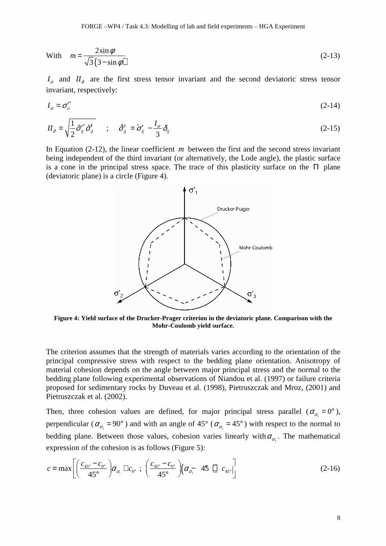
In Equation (2-12), the linear coefficient m between the first and the second stress invariant being independent of the third invariant (or alternatively, the Lode angle), the plastic surface is a cone in the principal stress space. The trace of this plasticity surface on the Π plane (deviatoric plane) is a circle (Figure 4).

Figure 4: Yield surface of the Drucker-Prager criterion in the deviatoric plane. Comparison with the

Mohr-Coulomb yield surface.

The criterion assumes that the strength of materials varies according to the orientation of the principal compressive stress with respect to the bedding plane orientation. Anisotropy of material cohesion depends on the angle between major principal stress and the normal to the bedding plane following experimental observations of Niandou et al. (1997) or failure criteria proposed for sedimentary rocks by Duveau et al. (1998), Pietruszczak and Mroz, (2001) and Pietruszczak et al. (2002).

Then, three cohesion values are defined, for major principal stress parallel (1

0σα = ° ),

perpendicular (1

90σα = ° ) and with an angle of 45° (1

45σα = ° ) with respect to the normal to

bedding plane. Between those values, cohesion varies linearly with1σα . The mathematical

expression of the cohesion is as follows (Figure 5):

( )1 1

45 0 45 00 45max ; 45

45 45

c c c cc c cσ σα α° ° ° °

° ° − − = + − ° + ° °

(2-16)


9

with 1σα being the angle between the normal to the bedding plane n

� and the major principal

stress 1σ� :

1

1

1

.arccos

n

nσσασ′ = ′

� �

� � (2-17)

Figure 5: Schematic view of the cohesion evolution as a function of the angle between the normal vector to

bedding plane and the direction of major principal stress.

In addition, a general non-associated plasticity framework is considered:

p Pij

ij

gε λσ

∗∗

∂=′∂

ɺ (2-18)

with the plastic potential g defined as:

ˆ 0g II m Iσ σ′≡ + = (2-19)

in which ( )2sin

3 3 sinm

ψψ

′ =−

(2-20)

where ψ is the dilatancy angle. When ψ φ= , ij ij

f g

σ σ∗ ∗

∂ ∂=′ ′∂ ∂

and the flow rule is associated.

The plastic multiplier pλ is obtained from the consistency condition, which states that during plastic flow the stress state stays on the limit surface:

0ijij

f fdf σ κ

σ κ∗

∗

∂ ∂′≡ + =′∂ ∂

ɺɺ (2-21)

with κ being the hardening variable(s). The used model is a hardening Drucker-Prager model that allows hardening/softening processes during plastic flow. This is introduced via an hyperbolic variation of the friction angle and the cohesion between initial (0φ and 0c ) and

final ( fφ and fc ) values as a function of the Von Mises equivalent plastic strain peqε

(Barnichon, 1998):


10

( )0

0

pf eq

pp eqB

φ φ εφ φ

ε−

= ++

(2-22)

( )0

0

pf eq

pc eq

c cc c

B

εε

−= +

+ (2-23)

where the Von Mises equivalent plastic strain peqε is obtained by integration of the Von Mises

equivalent plastic strain rate peqεɺ :

* *

0

2ˆ ˆ

3

tp p p p peq eq eq ij ijdtε ε ε ε ε= =∫ ɺ ɺɺ ɺ ; (2-24)

Coefficients pB and cB represent respectively the values of equivalent plastic strain for which

half of the hardening/softening on friction angle and cohesion is achieved (Figure 6). Thus, the consistency condition given in equation (2-21) reads:

0pij eqp p

ij eq eq

f f d f dcdf

d c d

φσ εσ φ ε ε

∗∗

∂ ∂ ∂ ′≡ + + = ′∂ ∂ ∂ ɺɺ (2-25)

Figure 6: Hardening/softening hyperbolic relation for 2 values of coefficient Bp

The Von Mises equivalent plastic strain can be expressed as a function of the plastic multiplier combining Equations (2-18) and (2-24), for the specific expression of the Drucker-Prager plastic potential (2-19):

2 1 3

3 3 3p P Peq

ij ij kk ll

g g g gε λ λσ σ σ σ∗ ∗ ∗ ∗

∂ ∂ ∂ ∂ = − = ′ ′ ′ ′∂ ∂ ∂ ∂

ɺ ɺɺ (2-26)

Combining together the elastic relation (2-8) and expression of plastic strain gives:

pij ijkl kl

kl

gCσ ε λ

σ∗ ∗

∗

∂ = − ′∂

ɺɺɺ (2-27)

That allows us to determine the plastic multiplier pλɺ :


11

33

eijkl kl

ijp

emnop p p

mn eq eq

fC

f f d f dcC

d c d

εσ

λφ

σ φ ε ε

∗∗

∗

∂′∂

=∂ ∂ ∂ − + ′∂ ∂ ∂

ɺ

ɺ (2-28)

2.2 Hydraulic anisotropy

Darcy’s law

The general Darcy flow law is used and defines the Darcy fluid velocity w

q as a linear

function of permeability and the gradient of fluid pressure wp :

( ) ( )int

.w

w www w

kKq p p

gρ µ= − ∇ = − ∇ (2-29)

where wK is the anisotropic tensor of permeability. This tensor has nine components and may

be written in a general form as follows:

xx xy xz

w yx yy yz

zx zy zz

K K K

K K K K

K K K

=

intk is the intrinsic permeability [m²] andwµ is the fluid dynamic viscosity [Pa/s].

k depends on the degree of saturation of the material:

r satk k k= (2-30)

with rk being the relative permeability coefficient defined by Marschall et al. (2005) for the

Opalinus Clay as:

( )22 0.51 (1 )rw r rk S S= − − (2-31)

where rS is the degree of saturation.

Retention curve

The degree of saturation is related to suction by the following expression:

112 2

11

CSR CSRw

r

pS

CSR

− − − = +

(2-32)

where CSR1 and CSR2 are material parameters.


12

Water specific mass

The water specific mass depends on pore water pressure:

00 1 w w

w ww

p pρ ρχ

−= +

(2-33)

where 0wρ is the reference water specific mass at reference pore water pressure wχ is the

liquid compressibility coefficient.

2.3 Balance equations

Momentum balance equation

The momentum balance equation is written for quasi-static conditions:

( ) 0ijdiv σ = (2-34)

where ijσ is the total stress tensor [Pa] expressed by:

ij ij r wb S pσ σ ′= − (2-35)

where b is the Biot coefficient and ijσ ′ the effective stress.

Water mass balance equation

We suppose that the water is only in the liquid phase. Then, the water mass balance equation can be written:

( ) ( ) w r w wwnS div q Q

tρ ρ∂ + =

∂ (2-36)

where w

q is the mean speed of the liquid phase compared to the solid phase [m.s-1] and wρ is

the bulk density of water [kg.m-3].

3 Model parameters identification 3.1 Mechanical parameter estimation from triaxial t ests

Laloui and François (2008) have compiled triaxial tests results corresponding to three different inclinations of the bedding plane with respect to the loading direction σ1 (Figure 7):

� Loading parallel to bedding planes: P-Sample, 1σα = 90°

� Loading perpendicular to bedding planes: S-Sample, 1σα = 0°

� Loading with an inclination of 45° to bedding planes: Z-Sample, 1σα = 45°

These triaxial tests have been performed under 4 different confinement pressures σ3 equal to: 0, 5, 10 and 15MPa (Figure 8). The geomechanical characteristics have been determined


13

through the comparison between these experimental results and their simulations based on the Drucker-Prager elastoplastic model without hardening/softening regimes.

Figure 7: Orientation of bedding with respect to the loading direction in P-, S- and Z- samples

Figure 8: Triaxial results under 4 different confinement pressures σ3 for three different inclinations of the bedding plane with respect to the loading direction σ1

Plastic parameter calibration

Assuming that plastic anisotropy only concerns cohesion parameter and not friction angle, the friction angle øc has been fixed to 20° in all directions as commonly admitted in literature. Cohesions are estimated from (p,q) graph drawn for each case (Figure 9). According to failure criteria given in equations (2-12) and (2-16) without taking into account hardening parameters in the behaviour, we obtain by considering only the most relevant (p,qfailure) points:

c0° = 6.4MPa, c45° =1.8MPa, c90° = 4.5MPa.


14

Figure 9: Failure criteria in (p, q) plane for three different inclinations of the bedding plane with respect to the loading direction σ1

Elastic parameter calibration

Identification of Poisson’s ratio can not be easily performed on triaxial test results. Its value with bedding orientation is chosen according to literature (Gens et al., 2007, Wileveau 2005, Martin and Lanyon 2003):

υ// // = 0.33 υ//⊥ = 0.24

Young’s modulus is identified on all triaxial tests. By averaging estimation for each loading case, we obtain the values summarized in Table 1 associated to numerical modelling results presented in Figure 10. They show that the elastic stiffness’s (and the corresponding shear strengths) are clearly affected by initial stress state as well as the direction of loading with respect to the bedding plane.


15

Figure 10: Triaxial tests calibrations under 4 different confinement pressures σ3 for three different inclinations of the bedding plane with respect to the loading direction σ1

Table 1: Young modulus identification on triaxial test with bedding orientation

σ3 [MPa] E// [GPa]

P-samples

E⊥⊥⊥⊥ [GPa]

S-samples

E45° [GPa]

Z-samples

0 3.2 2.2 2.3

5 4.6 3.5 3.2

10 5.9 4.9 4.1

15 7.2 6.2 4.0

3.2 Hydraulic parameters

The hydraulic parameters presented in Table 2 have been obtained from the literature (Gens et al., 2007, Wileveau 2005, Martin and Lanyon 2003). Table 2: Hydraulic characteristics

Initial porosity [-] n0 0.1

Initial intrinsic permeability [m²] ,//satk

,satk ⊥

2.10-20

8.10-21

Water specific mass [kg/m³] ρw 1000

Fluid dynamic viscosity [Pa.s] µw 10-3

Liquid compressibility coefficient [MPa-1] 1/χw 5.10-4

Coefficient of the water retention curve [MPa] CSR1 5

[-] CSR2 1.2


16

4 2D Modelling of tunnel excavation

Based on the in-situ measurements, the objective of the modelling of the excavation phase is to identify the concepts, the processes and the parameters of models in order to reproduce the creation and evolution of the EDZ. Also, these modelling will indicate the accuracy and the relevance of current models to predict EDZ structure.

4.1 Geometry, boundary conditions and loading descr iption

The HGA gallery has been excavated from a niche of the Gallery 04 of the Mont-Terri Underground Research Laboratory (URL). The drilling is parallel to the bedding orientation. In a section perpendicular to the gallery, the bedding plane is oriented at 45° with respect to horizontal direction (Figure 11).

Figure 11: Schematic view of the orientation of the HGA gallery with respect to bedding plane.

The problem has been considered as a 2D plane strain problem, considering a perpendicular section in the middle of the gallery. A 40m wide square domain has been considered. The initial stress is anisotropic:

� σZ = 6.5MPa (vertical stress),

� σX = 4.4MPa (horizontal radial stress)

� σY = 2.2MPa (horizontal axial stress)

The initial pore water pressure has been fixed to 0.9MPa. Because of the bedding anisotropy and the initial stress state does not follow the same orientation planes, the whole cross section needs to be taken into account in our model (no symmetry exists, see Figure 13).

In term of mechanical conditions, the external boundaries are kinematically constrained (no displacement). The internal boundary (at the gallery wall) is stress controlled. To simulate the excavation phase, the total stress at the gallery wall is decreased from the initial anisotropic stress to 0MPa within one day (86400s). The pore water pressure is maintained constant at 0.9MPa on the external boundaries while the pore water pressure at the gallery wall is reduced from 0.9MPa to 0MPa in 1 day (see Figure 12).

Afterward, a ventilation is put in place with a relative humidity RH = 83% and a temperature T = 13°C in average. To reproduce gallery ventilation, pore water pressure is linearly


17

decreased from 0 to a given suction in 7 days and then a constant pressure is maintained. Suction can be estimated as follow:

( )ln 23.9ww a

w

RTP P RH MPa

M

ρ− = = − (4-1)

Seepage elements are considered on the gallery wall to impose this relative humidity. That condition allows flow of water from the ground to the gallery (if the pore pressure of the ground is higher than the imposed pore pressure at the gallery wall) but restricts flow of water from the gallery to the ground.

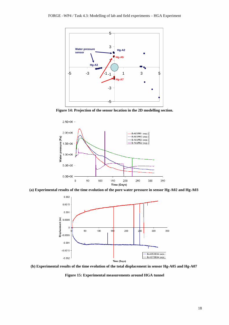
The hydro-mechanical response of Opalinus Clay around the excavated gallery has been simulated over a period of 322 days (from 18th February to 31st December 2005). The numerical results are compared with in-situ measurements in sensor HG-A2 and HG-A3 for pore water pressure and HG-A5 and HG-A7 for displacements. The locations of the sensors projected on one plane perpendicular to HGA borehole are reported in Figure 14. Pore water pressure and displacement evolutions with time measured in situ are drawn in Figure 15.

Figure 12: Hydromechanical loading (subtask 1)

Figure 13: Boundary conditions of the 2D plane strain model.

σy = 8MPa

σx = 3MPa

0 End of excavation End of excavation

Ventilation pressure is reached

0.9

0.1

Pw [MPa]

-24 days days


18

-5

-3

-1

1

3

5

-5 -3 -1 1 3 5

Hg-A3

Hg-A2

Hg-A5

Hg-A7

Water pressure sensor

-5

-3

-1

1

3

5

-5 -3 -1 1 3 5

-5

-3

-1

1

3

5

-5 -3 -1 1 3 5

Hg-A3

Hg-A2

Hg-A5

Hg-A7

Water pressure sensor

Figure 14: Projection of the sensor location in the 2D modelling section.

(a) Experimental results of the time evolution of the pore water pressure in sensor Hg-A02 and Hg-A03

(b) Experimental results of the time evolution of the total displacement in sensor Hg-A05 and Hg-A07

Figure 15: Experimental measurements around HGA tunnel


19

4.2 Hydromechanical parameters

The parameters consider in the Drucker-Prager elastoplastic model corresponds to the values identified on triaxial tests and summarized in Table 1 (for mechanical properties) and in Table 2 (for hydraulic properties). In this model, no hardening neither softening is included, which means that cohesion and friction angle do not evolve. No dilatancy is also taken into account. Furthermore, the model does not consider any evolution of Young’s modulus with stress state. Only one single value of E is included in each direction of anisotropy. By considering as initial stress the horizontal value σX = σ3 = 4.4MPa, the anisotropic values of E have been evaluated by linear interpolations of Table 1 estimations. Then, it follows: E// = 4.4GPa and E⊥= 3.3GPa. All the useful parameters are summarized in Table 3.

Table 3: Opalinus Clay parameters

Physical parameters

Initial porosity [-] n0 0.1

Volumic mass [kg/m³] ρ 2450

Water specific mass [kg/m³] ρw 1000

Water content [%] W 6.1

Fluid dynamic viscosity [Pa.s] µw 10-3

Liquid compressibility coefficient [MPa-1] 1/χw 5.10-4

Mechanical parameters

Young’s modulus [GPa] E//

E⊥

4.4

3.3

Poisson’s ratio [-] υ////

υ//⊥

0.33

0.24

Shear modulus [GPa] G////

G//⊥

1.6

1.3

Friction angle [°] øc 20

Cohesion [MPa]

c0°

c45°

c90°

6.4

1.8

4.5

Dilatancy [°] ψ 0

Biot coefficient [-] b 0.6

Hydraulic parameters

Initial intrinsic permeability [m²] ,//satk

,satk ⊥

2.10-20

8.10-21

Coefficient of the water retention curve [MPa] CSR1 5

[-] CSR2 1.2


20

4.3 Qualitative analysis of numerical results

4.3.1 Influence of anisotropic settings on global b ehaviour under purely mechanical conditions

In a first time, each kind of anisotropy is studied separately on a purely mechanical model of tunnel excavation (meaning that hydraulic variables are fixed). Then, it concerns analysis of the effects of initial stress anisotropy, Young’s modulus anisotropy and cohesion anisotropy on horizontal and vertical stresses and on plastic indicator. In a second time, analysis is extended to the combined effects of these three kinds of anisotropy.

Effect of initial stress anisotropy

In this mechanical modelling, parameters are assumed isotropic, meaning that Young’s modulus E is equal to 3.86GPa and Poisson’s ratio υ is equal to 0.28. Anisotropy only comes from initial stress conditions: σZ = 6.5MPa (vertical stress), σX = 4.4MPa (horizontal stress).

Tunnel excavation in these conditions provides an oval shape of tunnel due to stress redistribution corresponding to compression zone on horizontal axis and extension zone on vertical axis (Figure 16). As the vertical initial stress is higher than the horizontal one, plastic indicator describes an elliptic zone around tunnel for which the main orientation is horizontal. This plastic indicator is a reduced deviator equal to 1 if the current state is elasto-plastic (on the yield limit) and less than 1 otherwise (elastic behaviour). Maximal values reached are 0.817 horizontally and 0.257 vertically meaning that no plasticity is developed.

Horizontal stress Vertical stress

Plastic indicator

Figure 16: Effect of initial stress anisotropy on horizontal and vertical stresses and plastic indicator

0.235

[MPa]

-1.35

-6.30

[MPa]

0

-12.6

0.8


21

Effect of Young’s modulus anisotropy

In this mechanical modelling, initial stresses and Poisson’s ratio are assumed isotropic, meaning that σZ = σX = 4.4MPa and Poisson’s ratio υ is equal to 0.28. Anisotropy only comes from Young’s modulus: E// = 4.4GPa and E⊥ = 3.3GPa, oriented at 45°.

Tunnel excavation in these conditions provides slight oval shape of tunnel oriented at 45°, which is not sufficient to generate significant changes in stress redistributions. Stresses and plastic indicator are quite similar to cases without any anisotropy (Figure 17, plastic indicator is limited to 0.494).


Plastic indicator

Figure 17: Effect of Young modulus anisotropy on horizontal and vertical stresses and plastic indicator

Effect of cohesion anisotropy

In this mechanical modelling, initial stresses and Poisson’s ratio are assumed isotropic, meaning that σZ = σX = 4.4MPa and Poisson’s ratio υ is equal to 0.28. Anisotropy comes from Young’s modulus as previously: E// = 4.4GPa and E⊥ = 3.3GPa, oriented at 45°, and from plastic anisotropy through cohesion: c0° = 6.4MPa, c45° =1.8MPa and c90° = 4.5MPa.

As no plasticity is developed during excavation, stress redistribution around tunnel is similar to the previous case. Plastic indicator value is less than 1, however its distribution follows new orientations: maximal values are oriented along directions at 0° and 90°, minimal values are oriented along directions at ±45° (Figure 18).

[MPa]

-0.57

-7.50

[MPa]

-0.57

-7.50

0.455

0


22


Plastic indicator

Figure 18: Effect of cohesion anisotropy on horizontal and vertical stresses and plastic indicator

Combined effects of the three anisotropy sources

If the three sources of anisotropy are considered simultaneously, tunnel excavation provides an oval shape of tunnel oriented at +11° with the horizontal direction. However, stress redistribution directions are closed the horizontal one like in the case where initial stresses anisotropy is only considered. Effects of elasto-plastic anisotropy are too small to be significant on orientations; only a slight rotation can be noticed (Figure 19). However, elasto-plastic anisotropy influences the level of stress reached around excavation by intensifying the horizontal compression zone and the vertical extension zone. In term of plastic indicator, maximum value is reached and equal to 1 near the horizontal direction. It means that only the coupling between anisotropies of initial stresses, elastic and plastic parameters can provide plasticity in the model.

[MPa]

-0.57

-7.50

[MPa]

-0.57

-7.50

0.722

0


23


Plastic indicator

Deformed mesh

Figure 19: Simultaneous effect of initial stress, Young modulus and cohesion anisotropies on horizontal and vertical stresses, plastic indicator and deformed mesh

4.3.2 Influence of anisotropic settings on hydro-me chanical modelling

Previous calculations have been performed without taking into account hydraulic aspects. In this section, excavation and ventilation of the HGA borehole are modelled in order to put in evidence the effect of permeability and its anisotropy on hydro-mechanical modelling.

As described in section 4.1 and Figure 12, excavation modelling is performed in 24h. It is followed by ventilation phase. During 1 week, capillary pressure is reduced to reach -24MPa. Finally, pressure is kept constant for 10 months.

In a first analysis, no anisotropy is considered on permeability. Compare to previous calculation case, only hydraulic isotropic behaviour is added. It permits to put in evidence the effects of water and ventilation through water pressure and saturation degree on stress and strain fields and plastic indicator (Figure 20). In a second analysis, permeability anisotropy is included to capture its influence (Figure 21).

With isotropic hydraulic conditions

At the end of excavation phases: the presence of water generates a decrease of effective stresses and plastic criteria compare to previous cases, extending a little bit the plastic zone (Figure 20). On water pressure distribution, two zones with very high pressures can be

[MPa]

-1.24

-6.21

[MPa]

0

-10.9

1

0


24

distinguished. They correspond to the previous mechanical compression area. On contrary, in extension area, porosity increases and water pressure decreases. It results a small diminution of saturation degree and suction.

After 10 months of ventilation at 85% of relative humidity creates suction of -24MPa on the tunnel wall and the diminution of saturation degree. It provides an increase of effective stress all around the tunnel borehole. It is followed by a decrease of plastic indicator for which the maximal value is now equals to 0.773, meaning that no more plasticity is developed.

After excavation: After 10 months of ventilation:

Horizontal stress Horizontal stress

Vertical stress

Vertical stress

Plastic indicator

Plastic indicator

[MPa]

-1.02

-7.20

[MPa]

0

-10.5

[MPa]

-3.17

-9.52

[MPa]

0

-14.3

1

0

0.746

0.186


25

Water pressure

Water pressure

Saturation degree

Saturation degree

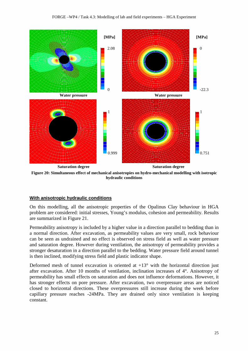
Figure 20: Simultaneous effect of mechanical anisotropies on hydro-mechanical modelling with isotropic hydraulic conditions

With anisotropic hydraulic conditions

On this modelling, all the anisotropic properties of the Opalinus Clay behaviour in HGA problem are considered: initial stresses, Young’s modulus, cohesion and permeability. Results are summarized in Figure 21.

Permeability anisotropy is included by a higher value in a direction parallel to bedding than in a normal direction. After excavation, as permeability values are very small, rock behaviour can be seen as undrained and no effect is observed on stress field as well as water pressure and saturation degree. However during ventilation, the anisotropy of permeability provides a stronger desaturation in a direction parallel to the bedding. Water pressure field around tunnel is then inclined, modifying stress field and plastic indicator shape.

Deformed mesh of tunnel excavation is oriented at +13° with the horizontal direction just after excavation. After 10 months of ventilation, inclination increases of 4°. Anisotropy of permeability has small effects on saturation and does not influence deformations. However, it has stronger effects on pore pressure. After excavation, two overpressure areas are noticed closed to horizontal directions. These overpressures still increase during the week before capillary pressure reaches -24MPa. They are drained only since ventilation is keeping constant.

[MPa]

2.08

0

1

0.999

[MPa]

0

-22.3

1

0.751


26

After excavation: After 10 months of ventilation:

Deformed mesh Deformed mesh

Horizontal stress Horizontal stress

Vertical stress

Vertical stress

Plastic indicator

Plastic indicator

[MPa]

-1.02

-7.20

[MPa]

0

-10.9

[MPa]

-0.65

-8.53

[MPa]

0

-13.1

1

0.2

0.202

0


27

Water pressure

Water pressure

Saturation degree Saturation degree Figure 21: Simultaneous effect of mechanical anisotropies on hydro-mechanical modelling with

anisotropic hydraulic conditions

4.3.3 Interpretation of numerical results

Because of the difference sources of anisotropy, the hydro-mechanical response of Opalinus Clay around the excavated gallery is not axisymmetric. The anisotropic stress state tends to induce two distinct behaviours on vertical and horizontal directions: an extensional behaviour (negative variation of pore water pressure) in the vertical direction and a compressive behaviour (positive variation of pore water pressure) in the horizontal direction (Figure 16). On the contrary, elastic anisotropy provokes higher variation of pore pressure in the stiffer direction (parallel to bedding) and less variation of pore pressure (or even negative variation) in the less rigid direction (perpendicular to bedding – Figure 20 ). Finally, anisotropic permeability makes drainage faster in the direction parallel to bedding (Figure 21). So, the combination of all sources of anisotropy makes complex the pore water pressure evolution.

Figure 21 shows the pore water pressure distribution at day 0 (immediately after excavation) and day 316, respectively. After one year of ventilation of the gallery, the negative pore water pressure propagates faster in the more permeable direction (parallel to bedding). The deformed mesh one year after the excavation presents minimum and maximum displacements occurring at 9° and 99° with respect to x axis, respectively. It corresponds to preferential directions in which plastic zone develops after excavation. Those directions correspond probably to the zone in which maximum shear stresses are concentrated. At the end of the simulation, the negative pore water pressure (suction) induced by the gallery ventilation provokes an increase in strength. As a consequence, the plastic processes are suppressed and the behaviour is elastic.

[MPa]

2.08

0

[MPa]

2

-22.7

1

0.999

1

0.740


28

Comparison with phenomena observed in situ

These previous numerical results can be compared to phenomena observed in situ. Figure 22 presents a picture of HGA borehole after excavation and its interpretation in term of damage. Two different damages can be distinguished:

� First, damage zones referred as “b” are slightly inclined to horizontal axis. They well correspond to plastic zones created after excavation as shown in Figure 21 or Figure 19. By analogy between plasticity and damage, the “b”-zones may be viewed as an excavation damaged zones due to mechanical anisotropy.

� Second, damage zones referred as “a” correspond to excavation shell at 45°, parallel to bedding, where water pressure and saturation degree decrease after excavation (see Figure 21). Stress modifications in this direction could reactivate bedding planes and generate some additional failures. The “a”-zones may be viewed as an excavation damaged zones due to hydraulic anisotropy effects. Remark that failure impact zone seems to be larger in the top than in the bottom on Figure 22 because of tectonic fault planes weakening the rock in a direction subparallel to bedding.

(a) (b)

Figure 22: (a) Picture of HGA borehole after excavation; (b) Schematic view of damage

Qualitatively, numerical results seem realistic and reliable to interpret observed phenomena. However quantitatively, comparison between experimental measurements and numerical results of water pressure evolution in the lateral HG-A3 borehole (Figure 23) shows that modelling is not sufficient to reproduce phenomena. Numerical simulation is able to reproduce the main trends of pore water pressure evolutions but some discrepancies between numerical and experimental results still exist. In fact, on one hand the intensity of the peak of the pore water pressure evolution measured by sensor HG-A3 is underestimated by the numerical simulations; on the other hand, the pore water pressure decrease after the peak is faster in the numerical simulations than in situ observed. Then, to improve the proposed 2D plane strain analysis, some complementary investigations are proposed in the following.


29

Figure 23: Water pressure evolution in HG-A3 borehole – comparison between experimental

measurements and numerical results

4.4 Complementary investigations for quantitative a nalysis

In order to improve the 2D plane strain numerical analysis of HGA microtunnel excavation, some complementary investigations are proposed based on the influences of mesh size, the presence of the main gallery or the creation of an excavation damaged zone.

4.4.1 Mesh sensitivity around HGA borehole

In the finite element analysis, some overpressures do not correspond to any physical effects but are the consequences of numerical instabilities, like oscillations, due to un-adapted mesh. As we have noticed a huge gradient of pore pressure on the first elements in contact with tunnel wall, several mesh sizes are studied to put in evidence whether previous results were perturbed or not by this kind of phenomena. From meshes corresponding to different degrees of refinement (see in Figure 24), analysis of water pressure field after 1 week of ventilation is proposed. Comparison of water pressure evolutions with time at 50cm to tunnel wall in the horizontal direction (that is to say closed to HG-A3 sensors borehole) for these 4 meshes can be shown in Figure 25.

These comparisons permit to illustrate that the global fine mesh (noted d) and the fine mesh around tunnel wall (noted c) provide the same water pressure evolution. On contrary, coarser meshes (noted a and b) provide overpressures with a “late-effect” in time. This confirms that even if in the previous analysis results (summarized in Figure 21) are qualitatively relevant, they are not quantitatively significant. Because of a strong gradient of water pressure close to tunnel wall, finite element model needs to admit a very fine mesh to better analyse the problem. Furthermore, the pore pressure level reached does not yet correspond to the measured one. Mesh size does not explain the intensity of the pore water pressure peak.


30

(a) (b)

(c) (d)

Figure 24: Pore pressure evolution after excavation depending of mesh size

Figure 25: Comparison of water pressure evolutions with time at 50cm to tunnel wall in the horizontal direction (HG-A3) for 4 different meshes

4.4.2 Influence of the lateral large gallery on HGA modelling

HGA microtunnel is closed and quite parallel to the main Gallery 04 of Mont Terri URL, which has been drilled 8 months before HGA microtunnel (see Figure 26). The short distance between HGA and the Gallery is expected to have effects on pore water pressure field. In fact, usually initial pore pressure in Mont Terri URL is equal to 2MPa, while around HGA

Por

e pr

essu

re (

MP

a)

0 50 100 150 200 250 300 350 400 days

mesh a

mesh b

meshes c & d

[MPa]

2.0

-2.0


31

microtunnel it has been measured equals to 0.9MPa. By including Gallery 04 in our model (considering a distance between HGA and the Gallery equals to 7.5m – see red box in Figure 26-a), the goal of this section is to evaluate its influence and to show if gallery drainage could explain the low water pressure value.

(a) (b)

Figure 26: Views of HGA microtunnel and Gallery04 in Mont Terri URL

Excavation and ventilation of Gallery04 during 8 mo nths

The main effects observed after excavation and ventilation of the Gallery04 are similar to the ones observed previously around HGA tunnel as shown on Figure 27. However, the specific shape of the gallery, provide some additional stress concentrations.

Because of the large scale of the excavated Gallery, ventilation and permeability anisotropy do not play a significant role on water pressures. Pressure field shape is not oriented parallel to bedding as around HGA borehole. Nevertheless, its extension is very large and includes microtunnel area, meaning that Gallery04 has an influence on HGA microtunnel environment. After 8 months of ventilation, water pressure in the neighbourhood of HGA microtunnel is around 0.9MPa, which is consistent with the measured value.

At the end of gallery excavation After 8 months of ventilation

Plastic indicator Plastic indicator

1

0.2

7.5m


32

Water pressure Water pressure

Figure 27: Results of Gallery04 modelling

Microtunnel modelling

After 8 months of ventilation, HGA microtunnel is drilled. During 1 year, no activity is realised despite tunnel ventilation. Then, a saturated backfill is put in place and we study its effect on pore pressure (Figure 28), saturation degree (Figure 29) and plastic indicator (Figure 30) during the 8 following years.

Even if qualitatively, results present in Figure 28, Figure 29 and Figure 30 are similar to the previous ones without gallery effects, evolution of water pressures with time (Figure 28) show that gallery excavation and drainage affect the water pressure evolution till the microtunnel area. Microtunnel is on the influence zone of Gallery04 drainage. However, it seems to not have influence on saturation degree; results on Figure 21 and Figure 29 are similar.

Plastic indicators are also similar (see Figure 21 and Figure 30): whereas after excavation plasticity appears, during the first year of ventilation plastic indicator decreases. After one year, saturated backfill installation keeps impermeable microtunnel wall. Suction is high, saturation degree increases and then plastic indicator evolves to reach a value close to 0.962. As water pressures are less than initial ones, no plasticity appears even after 9 years.

To conclude, the main effect of Gallery 04 is observed on water pressure evolutions. The measure value of initial pore pressure (before HGA microtunnel excavation) can be explained by Gallery04 drainage. One year after HGA microtunnel excavation, the global pore pressure stays constant and equal to 09.MPa. However, in the close neighbourhood of HGA microtunnel, pore pressure evolution is not significantly affect by Gallery04 drainage. Its influence is weak compare to the own microtunnel drainage to play a significant additional role on water pressure evolutions. Then, one can assume that it is not necessary to consider Gallery04 in the following.

5

0

[MPa]

1.35

-2.0

[MPa]


33

After microtunnel excavation After 1 year

After 2 years After 2 years (zoom)


Figure 28: Pore pressure evolutions around gallery04 and HGA microtunnel

2.5

-2

0.9

-0.9

[MPa]

0.9

-0.9

[MPa]

[MPa]

0.9

-0.9

[MPa]

0.9

-0.9

0.9

-0.9

[MPa]


34

After 1 year After 9 years

Figure 29: Saturation degree evolutions around HGA microtunnel (modelling accounting gallery effect)

After excavation After excavation (zoom)

After 1 year After 1 year (zoom)


Figure 30: Plastic indicator evolutions around gallery04 and HGA microtunnel

1

0.7

1

0.2

1

0.2

1

0.2


35

4.4.3 Introduction of an artificial EDZ around HGA borehole

Tunnel drilling provides stress redistribution and damage (microcracking), which reduce rock strength and increase permeability in a borehole surrounding area corresponding to the Excavation Damaged Zone. To take it into account in our approach, we propose to introduce an artificial EDZ through an ellipsoid defined thanks to an analogy between damage and plasticity as proposed in Figure 31. An example, we have chosen an ellipsoid centred on tunnel axis, for which the larger axis is 1.5m long oriented horizontally and the smaller axis is 0.75m long. In EDZ, Young modulus anisotropic values are divided by 100, whereas permeability anisotropic values are multiplied by 1000 compare to Table 3.

By introducing an EDZ, high vertical stress and large overpressures appear at the interface between EDZ and undamaged rock along the ellipsoid larger axis after excavation (see Figure 31 and Figure 32). It results two high values in the plastic indicator field in horizontal directions. More precisely, unloading due to excavation leads to vertical strains larger than the horizontal ones at the interface between intact rock and EDZ. Then, rock is in compression along larger ellipsoid axis because of EDZ contraction. This contraction can be explained by a decrease of water pressure in EDZ, in which permeability is very high. Deformed shape grows at the beginning of ventilation, increasing overpressures. When ventilation is stabilised, no more deformation appears and overpressures progressively decrease by EDZ drainage. However, one can notice that even if EDZ is oriented horizontally, drainage is influenced by permeability anisotropy at 45°.

Then, one can conclude that adding artificial EDZ around HGA borehole in FE modelling should be considered to explain the water pressure and displacement evolutions observed in situ (Figure 15). The next section 4.5 will be dedicated to its calibration.

At the end of excavation After 1 week

After 1 year

Figure 31: Water pressure evolution accounting EDZ

2.0

-2.0

[MPa]

2.0

-2.0

[MPa]


36

Vertical stress Plastic indicator

Figure 32: vertical stress and Plastic indicator evolutions accounting EDZ

4.5 Calibration on experimental results

According to Figure 31, the maximum of water pressure appears close to the extremity of EDZ-ellipsoid larger axis. Assuming that EDZ size is less than one tunnel radius and that HG-A3 sensors are outside EDZ, we have arbitrarily fixed ellipsoid size to 1m horizontally (half length of larger axis) and 0.57m vertically (half length of smaller axis). This corresponds to the area where plastic indicator is about 0.6 – 0.7 around tunnel without taking into account any EDZ. In these conditions, calibration is performed on displacement and water pressure measurements done on Figure 15.

To start calibration, only a reduced Young modulus is considered in EDZ. Permeability values are not modified. Using values of the 1st calibration in Table 4 provides displacements and pore water pressure fittings of Figure 33. It results that a modified value of Young modulus permits to well estimate displacements but is not sufficient to reproduce water pressure evolutions.

A second calibration is then proposed to take into account permeability evolution of about 5 orders of magnitude inside the EDZ (see Table 4). This permits to better fit experimental curves (Figure 34). However, calibration is not sufficient: displacements are overestimated and peaks of water pressure are not reproduced.

Table 4: Young modulus and Permeability calibrations

1st calibration 2nd calibration 3rd calibration 4th calibration

Outside

EDZ

Inside

EDZ

Outside

EDZ

Inside

EDZ

Outside

EDZ

Inside

EDZ

Outside

EDZ

Inside

EDZ

E// [GPa] 4.4 0.44 4.4 0.44 10 1 10 1

E⊥⊥⊥⊥ [GPa] 3.3 0.33 3.3 0.33 4 0.4 4 0.4

ksat // [m²] 2.10-20 2.10-20 2.10-20 2.10-15 2.10-20 2.10-15 8.10-21 8.10-16

ksat ⊥⊥⊥⊥ [m²] 8.10-21 8.10-21 8.10-21 8.10-16 8.10-21 8.10-16 3.210-21 3.210-16

0

-13

[MPa] 1.0

0.2


37

Figure 33: Displacements and Water pressures fitting by 1st calibration


38

Figure 34: Displacements and Water pressures fitting by 2nd calibration

To try to improve calibration, another way has been proposed. In this third calibration, anisotropic Young moduli of intact rock (outside EDZ) are fixed to values commonly used in literature: E// = 10GPa and E⊥= 4GPa. Inside the EDZ, Young modulus is divided by 10; a ratio of 105 is still chosen on permeability tensor (Table 4). By this way, displacement curve is better fitted as shown in Figure 35. Water pressure evolutions do not still reproduced peak magnitudes but show a realistic modification of slope at the beginning of ventilation phase.

Figure 35: Displacements and Water pressures fitting by 3rd calibration


39

Finally, a last calibration of permeability tensor (4th calibration in Table 4) provides a good compromise between displacements and water pressures fitting. In fact, dividing by 2.5 the permeability outside EDZ (intact rock) and multiplying by 105 the permeability inside EDZ permits to increase maximal overpressures without modifying significantly displacements as shown in Figure 36.

Figure 36: Displacements and Water pressures fitting by 4th calibration

4.6 Interpretation of calibrated numerical results

Figure 36 shows the rapid increase of pore water pressure in sensor HG-A3 while sensors HG-A2 measures a slight increase of pore water pressure. This difference in the pore water pressure response according to the radial direction of observation is due to the different sources of anisotropy (elastic, plastic, hydraulic and stress state). The main contribution of this difference is probably the anisotropy of the stress state. Vertical stress being much higher than horizontal stress, the gallery wall displacement is higher in the vertical direction, inducing a dilation of pore space along with a decrease of pore water pressure (sensor HG-A2). On the contrary, in the horizontal direction (sensor HG-A3), the behaviour is more compressive, inducing drastic increase of the pore water pressure.

The previous 2D plane strain numerical simulation is able to reproduce the main trends of pore water pressure evolutions. The introduction of a horizontal EDZ around HGA borehole permits to well capture the magnitude of the peak and the decrease which follows in the pore water pressure evolution measured by sensor HG-A3. The experimental measurement of the pore water pressure in sensor HG-A2 shows a slight increase of pore water pressure until 50


40

days after excavation while the numerical modelling predicts an immediate decrease of the pore water pressure. However, at long-term the same magnitude is reached.

Total displacement of sensor HG-A5 (1m above the gallery) and HG-A7 (1m below the excavation) show that after an immediate displacement 0.5mm, the displacements continue to increase due to consolidation processes. If the previous 2D plane strain numerical simulation is able to capture immediate response, the subsequent evolution of the displacements is slightly underestimated. The modelled displacements in sensor HG-A5 and HG-A7 are quite equal but opposite in sign. Anisotropy considered in the model is not sufficient to capture differences in these symmetric orientations (-90° and +90°).

Even if the 3D complex geometry of the system has been simplified into a 2D plane strain problem, the general trend of numerical results is in good agreement with experimental measurements. Nevertheless, new parameter calibration was necessary to capture good fittings.

However, these results have to be taken carefully. In 2D simulation, neither the effects of the impervious liner installed in the 6 first meters of the gallery nor the effects of excavation steps have been considered, even though they should have mechanical and hydraulic consequences on the global hydro-mechanical response. Moreover, all the sensors that are located in a 3D space have been projected in the 2D modelled plane, neglecting their longitudinal location. These assumptions let think that 2D plane strain model is still uncertain and need to be completed in future by 3D modelling.

5 Conclusions

The hydro-mechanical behaviour of Opalinus Clay around an excavated gallery has been numerically simulated through a 2D plane strain approach. To reproduce the dependency of the shear strength with the bedding orientation, an extended Drucker-Prager model with an anisotropic cohesion has been developed. The ability of that model to reproduce the behaviour of Opalinus Clay has been proved by numerical simulations of triaxial tests performed with different orientations of loading with respect to bedding plane and by numerical simulations of HGA microtunnel. However, analyses have put in evidence some numerical difficulties and the necessity to add complementary investigations on the presence of the main gallery or the creation of an excavation damaged zone around borehole. This has retarded the initial program, explaining why no numerical modelling relative to water and gas injection tests (subtasks 2 and 3) has been investigated yet.

Based on subtask 1 and the modelling of tunnel excavation, we have shown that the hydro-mechanical response of the Opalinus Clay around excavation is governed by four sources of anisotropy: the in-situ stress, the elastic modulus, the plastic yielding and the water permeability, keeping quite complex the global response of Opalinus Clay. Nevertheless, all the developments performed on HGA microtunnel numerical simulations show good agreement with available in-situ experimental measurements in term of displacement and water pressure evolutions.


41

6 References Barnichon J.D. (1998). Finite element modelling in structural and petroleum geology. PhD

Thesis, Université de Liège.

Drucker D.C., Prager W. (1952). Solid mechanics and plastic analysis for limit design. Quarterly of Applied Mathematics, vol. 10(2), pp. 157-165.

Duveau G., Shao J.F. and Henry J.P. (1998). Assessment of some failure criteria for strongly anisotropic geomaterials. Mechanics of cohesive-frictional materials, vol. 3, pp. 1-26.

Gens A., Vaunat J., Garitte B., Wileveau Y. (2007). In situ behaviour of a stiff layered clay subject to thermal loading: observations and interpretation. Geotechnique, vol. 57(2), pp. 207–228.

Graham J., Houlsby G.T. (1982) Anisotropic elasticity of a natural clay. Géotechnique, vol. 33(2), pp. 165-180.

Laloui L., François B. (2008). Benchmark on constitutive modeling of the mechanical behaviour of Opalinus Clay. Mont Terri Project, Technical Report.

Marschall P., Horseman S. and Gimmi T. (2005). Characterisation of Gas Transport Properties of the Opalinus Clay, a Potential Host Rock Formation for Radioactive Waste Disposal. Oil & Gas Science and Technology – Rev. IFP, vol. 60(1), pp. 121-139.

Martin C. D., Lanyon G. W. (2003) Measurement of in situ stress in weak rocks at Mont Terri Rock Laboratory, Switzerland. Int. J. Rock Mech. Mining Sci., vol. 40(7–8), pp. 1077–1088.

Niandou H., Shao J.F., Henry J.P., Fourmaintraux D. (1997). Laboratory investigations of the mechanical behaviour of Tournemire shale, Int. J. Rock Mech. Min. Sci., vol. 34, pp. 3-16.

Pietruszczak S., Mroz Z. (2001). On failure criteria for anisotropic cohesive-frictional materials. Int. J. Numer. Anal. Meth. Geomech., vol. 25, pp. 509-524.

Pietruszczak S., Lydzba D., Shao J.F. (2002). Modelling of inherent anisotropy in sedimentary rocks. Int. J. Solids and Structures, vol. 39, pp. 637-648.

Trick T., Marschall P., Rösli U., Lettry Y., Bossart P., Enachescu C. (2007). Instrumentation for a gas path through host rock and along sealing experiment. 7th International Symposium on Field Measurements in Geomechanics.

Wileveau Y. (2005). THM behaviour of host rock (HE-D) experiment: Progress report. Part 1, Technical Report TR 2005-03. Mont Terri Project.

Modelling of lab and field experiments HGA EXPERIMENT

Documents

Transcript of Modelling of lab and field experiments HGA EXPERIMENT