lable at ScienceDirect

Applied Geography 75 (2016) 28e35

Contents lists avai

Applied Geography

journal homepage: www.elsevier .com/locate/apgeog

Modelling of geographic cancer risk factor disparities in US counties*

Kyle D. BuckUS EPA/ORD/NHEERL/Gulf Ecology Division, 1 Sabine Island Drive, Gulf Breeze, FL 32561, USA

a r t i c l e i n f o

Article history:Received 18 August 2015Received in revised form29 July 2016Accepted 2 August 2016

Keywords:CancerMortality to incidence ratioGeographically weighted regressionSocialEconomicIndex

* A theoretical framework and geographic approcancer risk factor disparities in the United States.

E-mail address: buck.kyle@epa.gov.

http://dx.doi.org/10.1016/j.apgeog.2016.08.0010143-6228/© 2016 Published by Elsevier Ltd.

a b s t r a c t

The goal of this research is to create a theoretical framework for the identification of cancer risk factordisparities and address the recognition of geographic patterns in these factors. 34 secondary variablescovering the entire US at the county level in 2010 were analyzed, both individually and grouped(theoretically and statistically), in relation to the mortality to incidence ratio (MIR) for all cancer sites. Ana priori assessment and a principal components analysis (PCA) were used to group variables to testsocietal constructs. OLS and geographically weighted regressions (GWRs) were used to assess influenceof both individual and grouped variables against the MIR. The theoretical grouping of variables showedlittle change in predictive capability of OLS models. In GWR model, there was marked improvement overthe OLS. Maps produced using local R2 showed clear regional patterns of influence between the in-dicators and the MIR. Both the theoretical model and the justification for a spatial approach to cancer riskfactor disparities were shown to be effective in this paper. The link between this suite of indicators andthe health outcomes is clear, and supports the idea that a full representation of the SES landscape shouldbe used to both predict health outcomes and to assess policy options for improving these outcomes. Withthe presence of definitive regional patterns and clear connections between the MIR and societalgroupings, the findings from this research suggest a need to shift to a more comprehensive and spatialapproach to cancer disparities research.

© 2016 Published by Elsevier Ltd.

1. Introduction

The impact of cancer is enormous and takes a toll on both theindividual and societal level. The total US economic impact ofcancer in 2014 is estimated at $216.6 billion dollars, with nearly13.7 million people living with cancer, over 1.6 million diagnoses,andmore than half amillion deaths (Howlander, Noone,& Krapcho,2012; ACS, 2012). There is good news amidst the bad, however.Cancer incidence and mortality rates have been dropping in recentyears according to the American Cancer Society (ACS) along with 5-year survival rates, due in part to lifestyle improvements, moreadvanced treatment options, and earlier detection of many cancertypes (ACS, 2010).

Although the overall impact of cancer in the US looks to beheaded in the right direction, the effect is not felt equally among allgroups in the US. Cancer disparities, defined by National CancerInstitute (NCI), as “adverse differences in cancer incidence, cancer

ach to the identification of

prevalence, cancer death, cancer survivorship, and burden of canceror related health conditions that exist among specific populationgroups in the United States”, are becoming an increasing focus(National Health Disparities Act, 2000). As a result, NCI fundedprograms and research initiatives have aimed at the lack of cohe-sive analysis and clear frameworks by which disparities areassessed (Harper & Lynch, 2010). This paper proposes both atheoretical framework as well as a method of analysis intended tofill this identified gap.

In order to effectively address the cancer health disparities issue,a theoretical model is proposed that takes a more holistic approachto the assessment of social and economic constructs as they relateto cancer outcomes. This approach builds on previous research,which has concentrated predominantly on socioeconomic status(SES), race, ethnicity and gender differences as they relate to canceroutcomes (Calo, Suarez, Soto-Sal, gado, Quintana, & Ortiz, 2015;Cook et al., 2015; Hess, Lee, Fish, Daly, Cress, & Mayadev, 2015;Rizzo, Sherman & Arciero, 2015; Kim, Paik, Yoon, Lee, Kim & Sung,2015). Additional studies investigate the interaction of societalvariables that exists across communities and how other healthbehaviors influence specific cancer outcomes (Goovaerts et al.,2015; Kuo, Mobley & Anselin, 2011; Oliver, Smith, Siadaty, Hauck,

K.D. Buck / Applied Geography 75 (2016) 28e35 29

Pickle, 2006; Xiao, Gwede & Milla, 2007). Using a geographicapproach in the analysis of disparities, the aim of this research isultimately on the identification of regional trends and changes insocietal influence that lead to these differential impacts across allcancer types.

2. Materials and methods

2.1. Conceptual background

In order for any type of analysis to be successful, a solid theo-retical framework is required. In the case of cancer health dispar-ities, the framework proposed here will be based on the merging oftwo separate fields. The conceptual model of place-based healthvulnerability, shown in Fig. 1, forms the backbone of this researchand is significant in its combination of spatial methodologiesadopted from hazards geography and health disparities models(Cutter, 1996; Roux, 2012). By breaking apart each of the compo-nents of health risk, operationalization is possible along withmeasurement of each component's influence.

A big piece of this research lies in the correspondence of healthdisparities and hazards geography fields and what they areattempting to measure. Establishing the connection based on theconcept of vulnerability provides justification for the combinationof fields as well as the formation of a conceptual model merging thetwo. The link between cancer outcomes and geography has pro-vided further impetus into the development of newmodels for riskassessment (Lin, Schootman, & Zhan, 2015). In addition to this link,the ability to operationalize the model is of key concern, as it allowsfor the identification and measurement of cancer disparities basedon place and the measurement and comparison of the constructedfactors to the places with identified disparities.

Within the field of hazards geography, a great deal of researchhas been conducted on drivers of social vulnerability, with greatattention paid to the interaction of variables in space and time(Adger, 2006; Cutter, Mitchell, & Scott, 2000; Cutter, Boruff, &Shirley, 2003). What the hazards research has revealed is an intri-cate social structure with a high geographic dependence, whereone social factor does not always exert the same level of influenceon vulnerability. Utilizing the knowledge gained in the hazardsfield provides a much better metric for assessment of vulnerabilityto negative cancer outcomes. The outcomes as well as the drivers ofvulnerability between cancer and hazards are very similar andtreating the analysis of them similarly is a logical progression in theadvancement of cancer outcomes prediction.

Fig. 1. Place-based health vulnerability model.

In this conceptualization, vulnerability begins with the access,and health/behavior, and community/environmental characteris-tics, which interact to yield a baseline health risk. Variables used tomeasure these constructs are shown in the breakout boxes. Theresulting health risk is then filtered through the local social fabric toyield community health vulnerability, which will result in certaincancer outcomes and lead to potential disparities. Each factor inthis model has the potential to influence the other, and contributeto changes in the health vulnerability of a place. In this model, theshift in terminology from risk to vulnerability marks the change to aplace-based measurement, rather than an individual-basedmeasure.

Health disparities can stem from ethnic, gender, income, and agedivisions. In order to accurately reflect the influence of these, theanalysis must account for multiple combinations of variables thatcan exist amongst groups. Combinations of factors have been uti-lized in a few studies, but the scale has remained limited and only asmall number of variables are used in each case (Wagner et al.,2012; Li, Sunquist & Sunquist, 2012; Harper & Lynch, 2010). It isnot necessarily accurate to say a group is of a certain social class,and therefore more vulnerable. Other social indicators may exist,making them more or less vulnerable. For example, an individualmay be vulnerable due to their age, but this vulnerability could bedecreased if the individual is a wealthy, married female. Access tohealthy food options and green space can also influence the overallvulnerability (Bader, Purciel, Yousefzadeh, Neckerman, 2010; Dai,2011). Determining the relative impact of all cancer drivers inaddition to how these drivers interact with each other will allow fora much more thorough and accurate assessment of the sociallandscape and lead to better measurement of the drivers.

Cancer mortality-to-incidence ratios (MIR) are chosen as healthdisparity outcomes for a multitude of reasons. Cancer as anoutcome is relevant due to the large burden along with a well-researched history and established patterns of disparities amongcertain populations. The MIR measure represents potentiallyavoidable cancer deaths and has proven to be effective in control-ling for latency periods and relocation. It also helps to capture theearly detection of cancer and any effective treatment outcomes.Also, due to the interest in cancer disparities, the MIR is used tohelp isolate counties that are not receiving appropriate care, mostlikely due to differences in SES (Hebert et al., 2009; Wan, Zhan, Zou& Wilson, 2013).

The geographic analysis of cancer disparities is carried out inthis research using a geographically weighted regression (GWR)due to the demonstrated improvement in predictive ability of thesemodels in landscapes where characteristics are clustered (Kupfer &Farris, 2007; Zhao, Gao, Wang, Liu & Li, 2015; Fotheringham,Brundson, & Charlton, 2002). A GWR model allows for regressioncoefficients to vary by location, and thus helps to control for spatialnon-stationarity (Fotheringham et al., 2002; Legendre, 1993). Thecauses of cancer disparities will likely not be the same for all lo-cations, resulting in poor predictive models over the large spatialextent of the U.S. By using a GWR in addition to the proposedtheoretical framework for assessing cancer vulnerability, a picturecan be created that demonstrates large scale trends across the US.The regions where disparities are known to exist can be examinedin this larger context to better inform decisions related to thecauses of the disparities.

2.1.1. Data sourcesAll data collected for this research is freely available and

accessible. The temporal availability of each variable lies in therange of 2005e2010, with every attempt made to match the datefor accuracy of statistical analysis. Details for data sources alongwith dates can be found in Table 1. The data for outcome measures

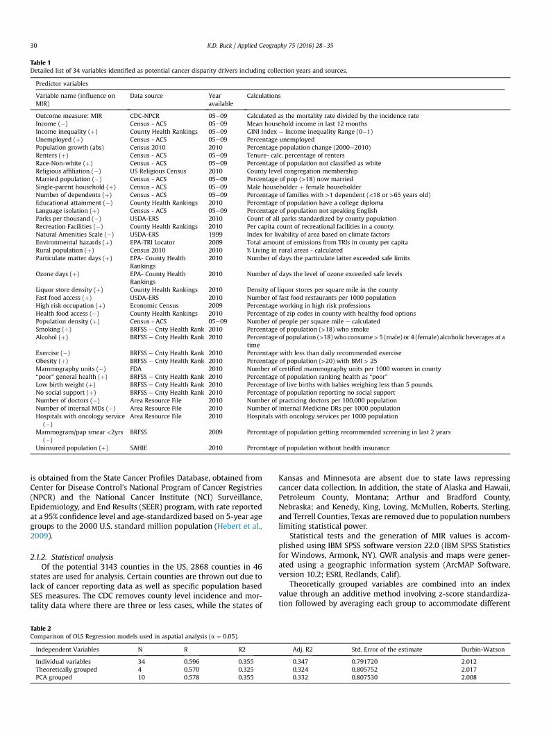
Table 1Detailed list of 34 variables identified as potential cancer disparity drivers including collection years and sources.

Predictor variables

Variable name (influence onMIR)

Data source Yearavailable

Calculations

Outcome measure: MIR CDC-NPCR 05e09 Calculated as the mortality rate divided by the incidence rateIncome (�) Census - ACS 05e09 Mean household income in last 12 monthsIncome inequality (þ) County Health Rankings 05e09 GINI Index e Income inequality Range (0e1)Unemployed (þ) Census - ACS 05e09 Percentage unemployedPopulation growth (abs) Census 2010 2010 Percentage population change (2000e2010)Renters (þ) Census - ACS 05e09 Tenure- calc. percentage of rentersRace-Non-white (þ) Census - ACS 05e09 Percentage of population not classified as whiteReligious affiliation (�) US Religious Census 2010 County level congregation membershipMarried population (�) Census - ACS 05e09 Percentage of pop (>18) now marriedSingle-parent household (þ) Census - ACS 05e09 Male householder þ female householderNumber of dependents (þ) Census - ACS 05e09 Percentage of families with >1 dependent (<18 or >65 years old)Educational attainment (�) County Health Rankings 2010 Percentage of population have a college diplomaLanguage isolation (þ) Census - ACS 05e09 Percentage of population not speaking EnglishParks per thousand (�) USDA-ERS 2010 Count of all parks standardized by county populationRecreation Facilities (�) County Health Rankings 2010 Per capita count of recreational facilities in a county.Natural Amenities Scale (�) USDA-ERS 1999 Index for livability of area based on climate factorsEnvironmental hazards (þ) EPA-TRI Locator 2009 Total amount of emissions from TRIs in county per capitaRural population (þ) Census 2010 2010 % Living in rural areas - calculatedParticulate matter days (þ) EPA- County Health

Rankings2010 Number of days the particulate latter exceeded safe limits

Ozone days (þ) EPA- County HealthRankings

2010 Number of days the level of ozone exceeded safe levels

Liquor store density (þ) County Health Rankings 2010 Density of liquor stores per square mile in the countyFast food access (þ) USDA-ERS 2010 Number of fast food restaurants per 1000 populationHigh risk occupation (þ) Economic Census 2009 Percentage working in high risk professionsHealth food access (�) County Health Rankings 2010 Percentage of zip codes in county with healthy food optionsPopulation density (þ) Census - ACS 05e09 Number of people per square mile e calculatedSmoking (þ) BRFSS e Cnty Health Rank 2010 Percentage of population (>18) who smokeAlcohol (þ) BRFSS e Cnty Health Rank 2010 Percentage of population (>18) who consume> 5 (male) or 4 (female) alcoholic beverages at a

timeExercise (�) BRFSS e Cnty Health Rank 2010 Percentage with less than daily recommended exerciseObesity (þ) BRFSS e Cnty Health Rank 2010 Percentage of population (>20) with BMI > 25Mammography units (�) FDA 2010 Number of certified mammography units per 1000 women in county“poor” general health (þ) BRFSS e Cnty Health Rank 2010 Percentage of population ranking health as “poor”Low birth weight (þ) BRFSS e Cnty Health Rank 2010 Percentage of live births with babies weighing less than 5 pounds.No social support (þ) BRFSS e Cnty Health Rank 2010 Percentage of population reporting no social supportNumber of doctors (�) Area Resource File 2010 Number of practicing doctors per 100,000 populationNumber of internal MDs (�) Area Resource File 2010 Number of internal Medicine DRs per 1000 populationHospitals with oncology service

(�)Area Resource File 2010 Hospitals with oncology services per 1000 population

Mammogram/pap smear <2yrs(�)

BRFSS 2009 Percentage of population getting recommended screening in last 2 years

Uninsured population (þ) SAHIE 2010 Percentage of population without health insurance

K.D. Buck / Applied Geography 75 (2016) 28e3530

is obtained from the State Cancer Profiles Database, obtained fromCenter for Disease Control's National Program of Cancer Registries(NPCR) and the National Cancer Institute (NCI) Surveillance,Epidemiology, and End Results (SEER) program, with rate reportedat a 95% confidence level and age-standardized based on 5-year agegroups to the 2000 U.S. standard million population (Hebert et al.,2009).

2.1.2. Statistical analysisOf the potential 3143 counties in the US, 2868 counties in 46

states are used for analysis. Certain counties are thrown out due tolack of cancer reporting data as well as specific population basedSES measures. The CDC removes county level incidence and mor-tality data where there are three or less cases, while the states of

Table 2Comparison of OLS Regression models used in aspatial analysis (a ¼ 0.05).

Independent Variables N R R2

Individual variables 34 0.596 0.355Theoretically grouped 4 0.570 0.325PCA grouped 10 0.578 0.355

Kansas and Minnesota are absent due to state laws repressingcancer data collection. In addition, the state of Alaska and Hawaii,Petroleum County, Montana; Arthur and Bradford County,Nebraska; and Kenedy, King, Loving, McMullen, Roberts, Sterling,and Terrell Counties, Texas are removed due to population numberslimiting statistical power.

Statistical tests and the generation of MIR values is accom-plished using IBM SPSS software version 22.0 (IBM SPSS Statisticsfor Windows, Armonk, NY). GWR analysis and maps were gener-ated using a geographic information system (ArcMAP Software,version 10.2; ESRI, Redlands, Calif).

Theoretically grouped variables are combined into an indexvalue through an additive method involving z-score standardiza-tion followed by averaging each group to accommodate different

Adj. R2 Std. Error of the estimate Durbin-Watson

0.347 0.791720 2.0120.324 0.805752 2.0170.332 0.807530 2.008

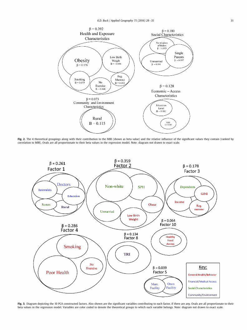
Fig. 2. The 4 theoretical groupings along with their contribution to the MIR (shown as beta value) and the relative influence of the significant values they contain (ranked bycorrelation to MIR). Ovals are all proportionate to their beta values in the regression model. Note: diagram not drawn to exact scale.

Fig. 3. Diagram depicting the 10 PCA constructed factors. Also shown are the significant variables contributing to each factor, if there are any. Ovals are all proportionate to theirbeta values in the regression model. Variables are color coded to denote the theoretical groups to which each variable belongs. Note: diagram not drawn to exact scale.

K.D. Buck / Applied Geography 75 (2016) 28e35 31

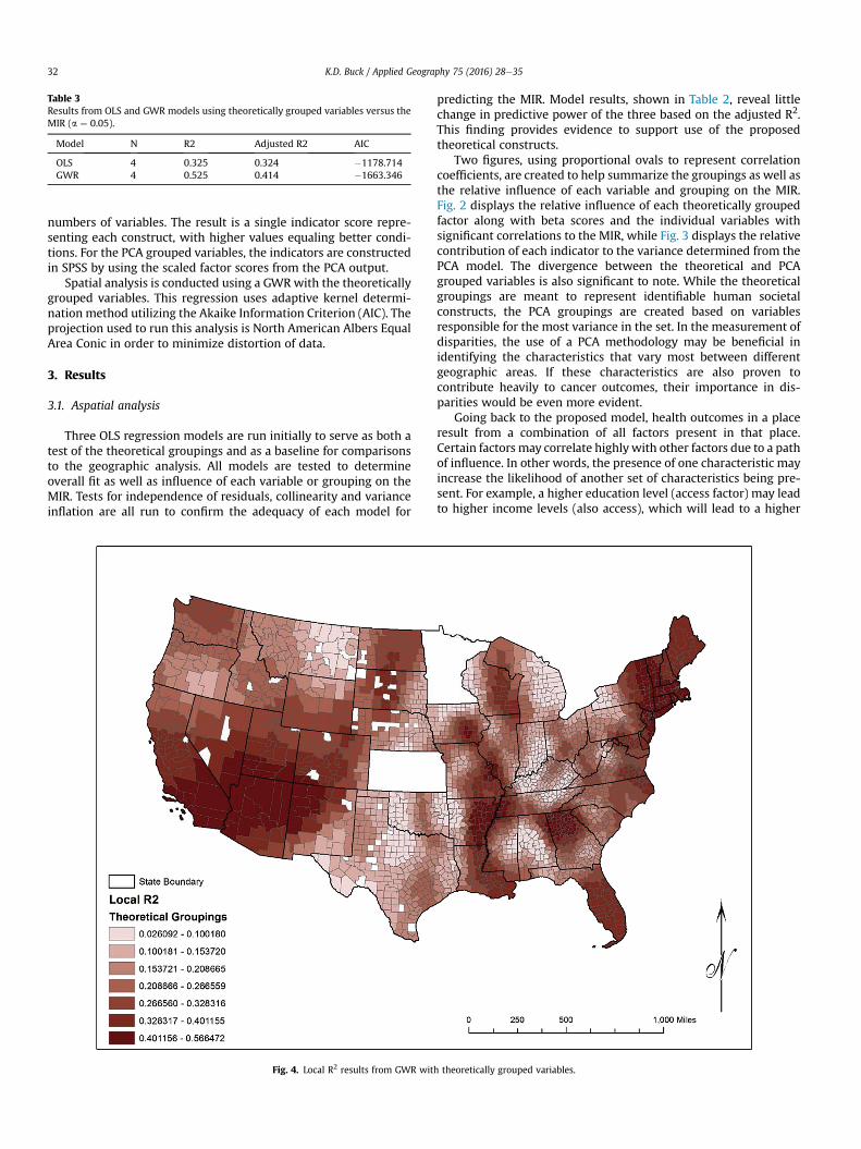
Table 3Results from OLS and GWR models using theoretically grouped variables versus theMIR (a ¼ 0.05).

Model N R2 Adjusted R2 AIC

OLS 4 0.325 0.324 �1178.714GWR 4 0.525 0.414 �1663.346

K.D. Buck / Applied Geography 75 (2016) 28e3532

numbers of variables. The result is a single indicator score repre-senting each construct, with higher values equaling better condi-tions. For the PCA grouped variables, the indicators are constructedin SPSS by using the scaled factor scores from the PCA output.

Spatial analysis is conducted using a GWRwith the theoreticallygrouped variables. This regression uses adaptive kernel determi-nation method utilizing the Akaike Information Criterion (AIC). Theprojection used to run this analysis is North American Albers EqualArea Conic in order to minimize distortion of data.

3. Results

3.1. Aspatial analysis

Three OLS regression models are run initially to serve as both atest of the theoretical groupings and as a baseline for comparisonsto the geographic analysis. All models are tested to determineoverall fit as well as influence of each variable or grouping on theMIR. Tests for independence of residuals, collinearity and varianceinflation are all run to confirm the adequacy of each model for

Fig. 4. Local R2 results from GWR wit

predicting the MIR. Model results, shown in Table 2, reveal littlechange in predictive power of the three based on the adjusted R2.This finding provides evidence to support use of the proposedtheoretical constructs.

Two figures, using proportional ovals to represent correlationcoefficients, are created to help summarize the groupings as well asthe relative influence of each variable and grouping on the MIR.Fig. 2 displays the relative influence of each theoretically groupedfactor along with beta scores and the individual variables withsignificant correlations to the MIR, while Fig. 3 displays the relativecontribution of each indicator to the variance determined from thePCA model. The divergence between the theoretical and PCAgrouped variables is also significant to note. While the theoreticalgroupings are meant to represent identifiable human societalconstructs, the PCA groupings are created based on variablesresponsible for the most variance in the set. In the measurement ofdisparities, the use of a PCA methodology may be beneficial inidentifying the characteristics that vary most between differentgeographic areas. If these characteristics are also proven tocontribute heavily to cancer outcomes, their importance in dis-parities would be even more evident.

Going back to the proposed model, health outcomes in a placeresult from a combination of all factors present in that place.Certain factors may correlate highlywith other factors due to a pathof influence. In other words, the presence of one characteristic mayincrease the likelihood of another set of characteristics being pre-sent. For example, a higher education level (access factor) may leadto higher income levels (also access), which will lead to a higher

h theoretically grouped variables.

Fig. 5. Local R2 results from GWR with theoretically grouped variables.

K.D. Buck / Applied Geography 75 (2016) 28e35 33

likelihood of access to recreational facilities and healthy food. All ofthis may result in a higher chance of exercising and eating well anda lower vulnerability to negative cancer outcomes. To summarize,even though the model constructs (factors) may be assembledaccurately, the relationship between the factors may be direction-ally dependent, meaning that one or more factors are ultimatelyresponsible for starting a chain of events that leads to higher cancerfatality rates. Ultimately, the results support the use of this theo-retical framework in assessing the influence of societal structuresvia theoretically grouped variables on cancer MIRs.

3.1.1. Spatial analysisThe outcomes of the GWR models for both the theoretically and

PCA grouped variables reveal improvements over the OLS models(Table 3). The adjusted R2 of the theoretically grouped OLS modelwas 0.325, whereas the GWR model produced an adjusted R2 of0.414. For the PCA grouped OLS model, the adjusted R2 was 0.332,while for the GWR model the adjusted R2 improved to a 0.417. Thisimprovement provides further evidence that spatial patterns are abetter predictor of cancer outcomes than using only aspatialmethods.

A major benefit of the GWR is the ability to visually representthe varying strength of relationship between the dependent andindependent variables by mapping the local R2 values. In this way,the explanatory strength can be tied to places. In Fig. 4, the varia-tion in local R2 values for the theoretically grouped variables isevident. The locations where the predictive values are strongestcorrespond with areas of both higher and lower MIR values as well,

indicating that this trend is not related solely to a better or worseoutcome. What it does signify is a strong regional trend. Fig. 5 re-veals a similar pattern in the PCA grouped variables, tying in theareas where variances are highest as well.

Looking at these two figures provides a clear depiction of thevarying relationship that exists between the SES of an area and thecancer outcomes for better or for worse. Regardless of the MIRvalues, there seems to be a presence of higher predictive statisticsin areas where populations are more concentrated. The northeast,for example, shows up as a place with higher predictive values. Inaddition to this, the Mississippi river corridor, Florida, the Atlantametro area, and the Southwest US all have higher local R2 values.This is significant, especially in the Southeast, due to the highernumbers of cancer fatalities that exist in this area. This regionpossesses many of the characteristics associated with poor cancerrates, and this shows up very clearly.

The most promising output from the GWR analysis comes fromthe individual regression outputs. Every county in the analysis hasits own regression equation, complete with local R2 values andcoefficients for each independent variable. These equations canprovide details on both the MIR as well as the level to which thesocietal structure influences this value. Even more detail may begleaned from the coefficients, which indicate the relative influenceof each construct on the MIR in that county. This output yieldsnumerous possibilities for future research. Table 4 provides a smallexample of data extracted from the analysis. In this table is thepredicted MIR as well as the measured MIR, along with all relevantinformation revealing strength of relationships between the

Table 4Example fromGWRmodel showing 4 counties. The observedMIR andmodel predictedMIR are shown alongwith the local R2 and the coefficients for each of the 4 theoreticallygrouped variables.

Observed MIR LocalR2 Predicted MIR Social Coeff. Health Coeff. Economic Coeff. Community Coeff.

3.903199 0.45625 2.70978 0.83920 0.58787 0.61050 �0.137383.565063 0.09086 0.24843 0.15098 0.66697 �0.00978 0.54660�1.351778 0.45395 �0.93240 0.16859 0.4052 0.64910 0.21508�2.449035 0.09192 �0.21783 0.55487 0.17388 �0.65367 0.81945

K.D. Buck / Applied Geography 75 (2016) 28e3534

indicators and the MIR. Two counties with high and two with lowMIR are shown. Each group has one county with high and one withlow local R2 as well. It is evident in just this small sample that theinfluence of each theoretical group on the MIR varies greatlydepending on location. This must be considered a major change inthe way these influences are analyzed.

4. Discussion

The primary outcome of this research is the establishment ofregional trends between MIRs and SES factors. Just as there is not asingle SES factor explaining cancer incidence or mortality rates,there also exists no single correlation among the regions. In otherwords, the linkage between SES factors andMIR in one place cannotbe assumed to exist in other places. There does appear to beregional clustering of the relationships, however, which impliesthat MIR outcomes and SES factors tend to vary in a manner thatcould be predicted. Given this information it would be possible tobetter identify the specific characteristics of a community thatpotentially drive poor cancer outcomes. In addition, there is reasonto look at more localized patterns, given appropriate data.

In addition to the spatial distribution among the MIR outcomesand SES factors, this research also demonstrates the benefit of atheoretical model for place-based assessment of cancer disparities.The model shows promise as a way to account for multiple com-ponents of social structure existing in a specific geography. Inaddition, it proves capable of operationalization for US counties,making possible the testing of multiple societal characteristics in acohesive manner. Dependent on data availability, this could alsotranslate to scaling at different levels.

Geographic regression models were shown to improve thepredictive capabilities by accounting for spatial non-stationaritythat existed in the data. This proves a definitive link between thecharacteristics of a place and the change in how certain predictorvariables influence cancer outcomes and implies that smaller casestudies are not applicable to other places where influences may notbe the same. Having a country wide analysis of this regional vari-ance should prove very helpful in making comparisons across casestudies in the future.

Lastly, this research shows promise in the identification ofspatial cancer disparities and the ability to identify sets of com-munity characteristics linked to them. The ability to break downand analyze individual places and quantify the link between amultitude of characteristics and cancer outcomes could be veryhelpful in justifying the location of specific services known to helpdecrease cancer rates.

5. Conclusion

The policy implications of this research are broad reaching andhave the potential to aid in the identification of places where notonly disparities exist, but also the reasons why they exist. A majorgoal that has carried through each iteration of the Healthy Peopleinitiative is the reduction/elimination of disparities. In order toaccomplish this goal, both the location of the disparities as well as

and understanding of the drivers is necessary. Removing obstaclesto proper health care and equitable health outcomes is critical, andunderstanding how these obstacles present themselves in a place isessential to achieving the goal of Healthy People, 2020 (HealthyPeople, 2015).

Hopefully the findings in this paper will begin to address theneed for identification of both the fundamental drivers of cancerdifferences and the regional patterns that impact how societaldrivers actually affect cancer outcomes in a specific place. Asopposed to working from the bottom up, starting with smallerspatial studies, the work presented here attempts a top downapproach by creating a country-wide look at disparities and theirdrivers. With this overview, smaller scale studies can be bettersituated in relation to others and better predictions made.

References

ACS, A. C. S. (2010). Cancer facts& figures 2010. Atlanta, GA: American Cancer SocietyACS.

ACS, A. C. S. (2012). Cancer facts & figures 2012. Atlanta, GA.Adger, W. N. (2006). Vulnerability. Global Environmental Change-Human and Policy

Dimensions, 16(3), 268e281.Bader, M. D. M., Purciel, M., Yousefzadeh, P., & Neckerman, K. M. (2010). Disparities

in neighborhood food environments: Implications of measurement strategies.Economic Geography, 86(4), 409e430.

Calo, W. A., Suarez, E., Soto-Salgado, M., Quintana, R. A., & Ortiz, A. P. (2015).Assessing lung cancer incidence disparities between Puerto Ricans and otherRacial/Ethnic Groups in the United States, 1992-2010. Journal of Immigrant andMinority Health, 17(3), 971e975. http://dx.doi.org/10.1007/s10903-014-0153-1.

Cook, M. B., Rosenberg, P. S., McCarty, F. A., Wu, M. X., King, J., Eheman, C., et al.(2015). Racial disparities in prostate cancer incidence rates by census division inthe United States, 1999-2008. Prostate, 75(7), 758e763. http://dx.doi.org/10.1002/pros.22958.

Cutter, S. L. (1996). Vulnerability to environmental hazards. Progress in HumanGeography, 20(4), 529e539. http://dx.doi.org/10.1177/030913259602000407.

Cutter, S. L., Boruff, B. J., & Shirley, W. L. (2003). Social vulnerability to environ-mental hazards. Social Science Quarterly, 84(2), 242e261.

Cutter, S. L., Mitchell, J. T., & Scott, M. S. (2000). Revealing the vulnerability of peopleand places: A case study of Geogretown County, South Carolina. Annals of theAssociation of American Geographers, 90(4), 713e737.

Dai, D. (2011). Racial/ethnic and socioeconomic disparities in urban green spaceaccessibility: Where to intervene? Landscape and Urban Planning, 102(4),234e244.

Fotheringham, A. S., Brundson, C., & Charlton, M. (2002). Geographically weightedregression: The analysis of spatially varying relationships. Wiley.

Goovaerts, P., Hong, X., Adunlin, A., Ali, A., Tan, F., Gwede, C. K., et al. (2015).Geographically-weighted regression analysis of percentage of late-stage pros-tate cancer diagnosis in Florida. Applied Geography, 62, 191e200.

Harper, S., & Lynch, J. (2010). Methods for measuring Cancer Disparities: Using datarelevant to healthy people 2010 Cancer-Related objectives. In NCI Cancer sur-veillance monograph series (Vol. 6). The National Cancer Institute.

Healthy People 2020 [Internet]. Washington, DC: U.S. Department of Health andHuman Services, Office of Disease prevention and health promotion [citedAugust 11, 2015], 2015, Available from:: [https://www.healthypeople.gov/2020/about/foundation-health-measures/Disparities].

Hebert, J. R., Daguise, V. G., Hurley, D. M., et al. (2009). Mapping cancer mortality-to-incidence ratios to illustrate racial and sex disparities in a high-risk popu-lation. Cancer, 115(11), 2539e2552.

Hess, C., Lee, A., Fish, K., Daly, M., Cress, R. D., & Mayadev, J. (2015). Socioeconomicand Racial Disparities in the Selection of Chest Wall Boost Radiation Therapy inCalifornian Women After Mastectomy. Clinical Breast Cancer, 15(3), 212e218.http://dx.doi.org/10.1016/j.clbc.2014.11.007.

Howlander, M., Noone, A. M., & Krapcho, M. (2012). SEER Cancer statistics review,1975-2009. National Cancer Institute.

Kim, S. E., Paik, H. Y., Yoon, H., Lee, J. E., Kim, N., & Sung, M. K. (2015). Sex- andgender-specific disparities in colorectal cancer risk. World Journal of Gastroen-terology, 21(17), 5167e5175. http://dx.doi.org/10.3748/wjg.v21.i17.5167.

K.D. Buck / Applied Geography 75 (2016) 28e35 35

Kuo, T. M., Mobley, L. R., & Anselin, L. (2011). Geographic disparities in late-stagebreast cancer diagnosis in California. Health & Place, 17(1), 327e334.

Kupfer, J. A., & Farris, C. A. (2007). Incorporating spatial non-stationarity ofregression coefficients into predictive vegetation models. Landscape Ecology,22(6), 837e852. http://dx.doi.org/10.1007/s10980-006-9058-2.

Legendre, P. (1993). Spatial autocorrelation - Trouble or new paradigm. Ecology,74(6), 1659e1673. http://dx.doi.org/10.2307/1939924.

Lin, Y., Schootman, M., & Zhan, F. B. (2015). Racial/ethnic, area socioeconomic, andgeographic disparities of cervical cancer survival in Texas. Applied Geography,56, 21e28. http://dx.doi.org/10.1016/j.apgeog.2014.10.004.

Li, X. L., Sunquist, K., & Sunquist, J. (2012). Neighborhood deprivation and prostatecancer mortality: A multilevel analysis from Sweden. Prostate Cancer andProstatic Diseases, 15(2), 128e134.

Minority Health and Health Disparities Research and Education Act of 2000, 106U.S.C. x 1880, 2000, Retrieved from https://www.congress.gov/bill/106th-congress/senate-bill/1880/.

Oliver, N. M., Smith, E., Siadaty, M., Hauck, F. R., & Pickle, L. W. (2006). Spatialanalysis of prostate cancer incidence and race in Virginia, 1990-1999. AmericanJournal of Preventive Medicine, 30(2), S67eS76.

Rizzo, J. A., Sherman, W. E., & Arciero, C. A. (2015). Racial disparity in survival from

early breast cancer in the department of defense healthcare system. Journal ofSurgical Oncology, 111(7), 819e823. http://dx.doi.org/10.1002/jso.23884.

Roux, A. V. D. (2012). Conceptual approaches to the study of health disparities. InJ. E. Fielding (Ed.), Annual review of public health (Vol. 33, pp. 41e58). Palo Alto:Annual Reviews.

Wagner, S. E., Hurley, D. M., Hebert, J. R., McNamara, C., Bayakly, A. R., & Vena, J. E.(2012). Cancer mortalityto-incidence ratios in Georgia describing racial cancerdisparities and potential geographic determinants. Cancer, 118(6), 4032e4045.

Wan, N., Zhan, F. B., Zou, B., & Wilson, J. G. (2013). Spatial access to health careservices and disparities in colorectal cancer stage at diagnosis in Texas. Pro-fessional Geographer, 65(3), 527e541. http://dx.doi.org/10.1080/00330124.2012.700502.

Xiao, H., Gwede, C. K., & Milla, K. (2007). Analysis of prostate cancer incidence usinggeographic information system and multilevel modeling. Journal of the NationalMedical Association, 99(3), 218.

Zhao, Z. Q., Gao, J. B., Wang, Y. L., Liu, J. G., & Li, S. C. (2015). Exploring spatiallyvariable relationships between NDVI and climatic factors in a transition zoneusing geographically weighted regression. Theoretical and Applied Climatology,120(3e4), 507e519. http://dx.doi.org/10.1007/s00704-014-1188-x.