MODELLING OF BIOLOGICAL SYSTEMS - MPI-CBG · method. One often hears that this is because...

Section IV

MODELLING OFBIOLOGICAL SYSTEMS

3rd Readingb711_Chapter-14.qxd 2/27/2009 4:04 PM Page 379

381

3rd Reading

Chapter 14

Spatiotemporal Modelingand Simulation in Biology

Ivo F. Sbalzarini

1. Introduction

Describing the dynamics of processes in both space and time simultane-ously is referred to as spatiotemporal modeling. This is in contrast todescribing the dynamics of a system in time only as is, for example, usu-ally done in chemical kinetics or pathway models. Solving spatiotempo-ral models in a computer requires spatiotemporal computer simulations.While computational data analysis allows unbiased and reproducible pro-cessing of large amounts of data from, e.g. high-throughput assays,computer simulations enable virtual experiments in silico that would notbe possible in reality. This greatly expands the range of possible pertur-bations and observations. Computational experiments allow studyingsystems whose complexity prohibits manual analysis, and they makeaccessible time and length scales that cannot be reached by lab experi-ments. Examples of the latter include molecular dynamics (MD) studiesin structural biology and studies in ecology or evolutionary biology.In virtual experiments, all variables are controllable and observable.We can thus measure everything and precisely control all influences and cross-couplings. This allows disentangling coupled effects that could not beseparated in real experiments, greatly reduces or eliminates the need forindirect control experiments, and facilitates interpretation of the results.Finally, computational models do not involve living beings, thus enabling

b711_Chapter-14.qxd 2/27/2009 4:04 PM 81

experiments that would not be possible in reality due to ethical reasons.Although we focus on applications of spatiotemporal computer simula-tions in biology, the employed concepts and methods are more gener-ally valid.

Resolving a dynamic process in space greatly increases the number ofdegrees of freedom (variables) that need to be tracked. Consider, forexample, a biochemical heterodimerization reaction. This reaction can bemodeled by its chemical kinetics using three variables: the concentrationsof the two monomers and the concentration of dimers. Assume now thatmonomers are produced at certain locations in space and freely diffusefrom there. Their concentration thus varies in space in such a way that itis higher close to the source and lower farther away, which greatlyincreases the number of variables we have to track in the simulation.If we are, say, interested in the local concentrations at 1000 positions, wealready have to keep track of 3000 variables. Moreover, the reactions tak-ing place at different points in space are not independent. Each localreaction can influence the others through diffusive transport ofmonomers and dimers. The complexity of spatiotemporal models thusrapidly increases. In fact, there is no theoretical limit to the number ofpoints in space that we may use to resolve the spatial patterns in the con-centration fields. Using infinitely many points corresponds to modelingthe system as a continuum.

A number of powerful mathematical tools are available to efficientlydeal with spatiotemporal models and to simulate them. While it is notpossible within the scope of this chapter to describe each of them indetail, we will give an overview with references to specialized literature.We then review in detail one particular method that is well suited forapplications in biology. But before we start, we revisit some of the moti-vations and particularities of spatiotemporal modeling in the life sciences.

In spatiotemporal modeling, nature is mostly described in fourdimensions: time plus three spatial dimensions. While time and the pres-ence of reservoirs (integrators) are essential for the existence of dynam-ics, three-dimensional (3D) spatial aspects also play important roles inmany biological processes. Think, for example, of predators hunting theirprey in a forest, of blood flowing through our arteries, of the electro-magnetic fields in the brain, or of such an unpleasant phenomenon as the

382 I. F. Sbalzarini


epidemic spread of a disease. In all of these examples, and many others,the spatial distributions of some quantities play an essential role. Modelsand simulations of such systems should thus account for and resolve thesedistributions. When determining the location of an epileptic site in thebrain, it is, for instance, of little value to know the total electric currentdensity in the whole brain — we need to know precisely where the sourceis. These examples extend across all scales of biological systems, from theabove-mentioned predator–prey interactions in ecosystems over mor-phogenesis1–5 and intracellular processes to single molecules. Think,for example, of conformational changes in proteins. Examples atthe intracellular level include virus entry6,7 and transport,8–10 intracellularsignaling,11,12 the diffusion of proteins in the various cellular compart-ments,13–15 or the fact that such compartments exist in the first place.

Spatial organization is important, as the same protein can have dif-ferent effects depending on the intracellular compartment in which it islocated. The most prominent example is probably cytochrome C, whichis an essential part of the cell respiration chain in the mitochondria, buttriggers programmed cell death (apoptosis) when released into the cyto-plasm.16 Another example is found in the role of transmembrane signal-ing during morphogenesis. Differences in protein diffusion constants arenot large enough to produce Turing patterns,1 and the slow transportacross intercompartment membranes is essential.17 Examples of spatiotem-poral processes at the multi-cellular level include tumor growth18–20 andcell-cell signaling,21 including phenomena such as bacterial quorum sens-ing, the microscopic mechanism underlying the macroscopic phenome-non of bioluminescence in certain squid.22

Given the widespread importance of spatiotemporal processes, it isnot surprising that a number of large software projects for spatiotempo-ral simulations in biology have been initiated. Examples in computationalcell biology23,24 include E-Cell, MCell, and the Virtual Cell.

2. Properties of Biological Systems

Simulating spatially resolved processes in biological systems, such asgeographically structured populations, multicellular organs, or cellorganelles, provides a unique set of challenges to any mathematical

Spatiotemporal Modeling and Simulation in Biology 383


method. One often hears that this is because biological systems are“complex”.

Biochemical networks, ecosystems, biological waves, heart cell syn-chronization, and life in general are located in the high-dimensional,nonlinear regime of the map of dynamical systems,25 together with quan-tum field theory, nonlinear optics, and turbulent flows. None of thesetopics are completely explored. They are at the limit of our currentunderstanding and will remain challenging for many years to come. Whyis this so, and what do we mean by “complex”?

Biological systems exhibit a number of characteristics that render themdifficult. These properties frequently include one or several of the following:

• high-dimensional (or infinite-dimensional in the continuum limit);• regulated;• delineated by complex shapes;• nonlinear;• coupled across scales and subsystems;• plastic over time (time-varying dynamics); and/or• nonequilibrium.

Due to these properties, biological systems challenge existing meth-ods in modeling and simulation. They are thus particularly well suited todrive the development of new methods and theories. The challenges pre-sented by spatiotemporal biological systems have to be addressed on sev-eral fronts simultaneously: numerical simulation methods, computationalalgorithms, and software engineering.26 Numerical methods are neededthat can deal with multi-scale systems27–31 and topological changes incomplex geometries. Computer algorithms have to be efficient enoughto deal with the vast number of degrees of freedom, and software plat-forms must be available to effectively and robustly implement thesealgorithms on multiprocessor computers.32

2.1. Dimensionality and Degrees of Freedom

The large number of dimensions (degrees of freedom) is due to the fact thatbiological systems typically contain more compartments, components, and



interaction modes than traditional engineering applications such as elec-tronic circuits or fluid mechanics.26 In a direct numerical simulation, alldegrees of freedom need to be explicitly tracked. In continuous systems,each point in space adds additional degrees of freedom, leading to an infi-nite number of dimensions. Such systems have to be discretized, i.e. thenumber of degrees of freedom needs to be reduced to a computationallyfeasible amount, which is done by selecting certain representative dimen-sions. Only these are then tracked in the simulation, approximating thebehavior of the full, infinite-dimensional system. Discretizations must beconsistent, i.e. the discretized system has to converge to the full systemif the number of explicitly tracked degrees of freedom goes to infinity.

Discrete biological systems already have a finite number of degrees offreedom and can sometimes be simulated directly. If the number of degreesof freedom is too large, as is e.g. the case when tracking the motion of allatoms in a protein, we do, however, again have to reduce them in orderfor simulations to be feasible. This can be done by collecting severaldegrees of freedom into one and only tracking their collective behavior.These so-called “coarse graining” methods greatly reduce the computa-tional cost and allow simulations of very large, high-dimensional systemssuch as patches of lipid bilayers with embedded proteins,33,34 or actin fil-aments.35 Coarse graining thus allows extending the capabilities ofmolecular simulations to time and length scales of biological interest.

2.2. Regulation

In biological systems, little is left to chance, which might seem surprisinggiven the inherently stochastic nature of molecular processes, environ-mental influences, and phenotypic variability. These underlying fluctua-tions are, however, in many cases a prerequisite for adaptive deterministicbehavior, as has been shown, for example, in gene regulation networks.36

In addition to such indirect regulation mediated by bistability and sto-chastic fluctuations, feedback and feed-forward loops are ubiquitous inbiological systems. From signal transduction pathways in single cells toDarwinian evolution, regulatory mechanisms play important roles.Results from control theory tell us that such loops can alter the dynamicbehavior of a system, change its stability or robustness, or give rise to



multi-stable behavior that enables adaptation to external changes anddisturbances.36 Taking all of these effects into account presents a grandchallenge to simulation models not only because many of the hypotheti-cal regulatory mechanisms are still unknown or poorly characterized.

2.3. Geometric Complexity

Biological systems are mostly characterized by irregular and often mov-ing or deforming geometries. Processes on curved surfaces may be cou-pled to processes in enclosed spaces; and surfaces frequently change theirtopology, such as in fusion or fission of intracellular compartments.Examples of such complex geometries are found on all length scales andinclude the prefractal structures of taxonomic and phylogenetic trees,37

regions of stable population growth in ecosystems,38 pneumonal andarterial trees,39 the shapes of neurons,40 the cytoplasmic space,41 clustersof intracellular vesicles,42 electric currents through ion channels in cellmembranes,43 protein chain conformations,44 and protein structures.45

Complex geometries are not only difficult to resolve and represent in thecomputer, but the boundary conditions imposed by them on dynamicspatiotemporal processes may also qualitatively alter the macroscopicallyobserved dynamics. Diffusion in complex-shaped compartments such asthe endoplasmic reticulum (ER; Fig. 1) may appear anomalous, even ifthe underlying molecular diffusion is normal.46–49

2.4. Nonlinearity

Common biological phenomena such as interference, cooperation, andcompetition lead to nonlinear dynamic behavior. Many processes, fromrepressor interactions in gene networks over predator–prey interactionsin ecosystems to calcium waves in cells, are not appropriately describedby linear systems theory as predominantly used and taught in physics andengineering. Depending on the number of degrees of freedom, nonlin-ear systems exhibit phenomena not observed in linear systems. Thesephenomena include bifurcations, nonlinear oscillations, and chaos andfractals. Nonlinear models are intrinsically hard to solve. Most of them areimpossible to solve analytically; and computer simulations are hampered



by the fact that common computational methods, such as normal modeanalysis, Fourier transforms, or the superposition principle, break downin nonlinear systems because a nonlinear system is not equal to the sumof its parts.25

2.5. Coupling Across Scales

Coupling across scales means that events on the microscopic scale suchas changes in molecular conformation can have significant effects on theglobal, macroscopic behavior of the system. This is certainly the case formany biological systems — bioluminescence due to bacterial quorumsensing22 for example, or the effect on the behavior of a whole organismwhen hormones bind to their receptors. Such multi-scale systems sharethe property that the individual scales cannot be separated and treatedindependently. There is a continuous spectrum of scales with coupledinteractions that impose stringent limits on the use of computer simu-lations. Direct numerical simulation of the complete system wouldrequire resolving it in all detail everywhere. Applied to the simulation ofa living cell, this would mean resolving the dynamics of all atoms in thecell. A cell consists of about 1015 atoms, and biologically relevantprocesses such as protein folding and enzymatic reactions occur onthe time scale of milliseconds. The largest molecular dynamics (MD)50


3rd Reading

Fig. 1. (a) Shaded view of a 3D computer reconstruction of the geometry of anendoplasmic reticulum (ER) of a live cell.49 (b) Close-up of a reconstructed ER, illus-trating the geometric complexity of this intracellular structure.

b711_Chapter-14.qxd 2/27/2009 4:04 PM Page 387

simulations currently done consider about 1010 atoms over one nanosecond.In order to model a complete cell, we would need a simulation about100 000 times larger, running over a millionfold longer time interval.This would result in a simulation at least 1011 times bigger than what cancurrently be done. This is certainly not feasible and will remain so formany years to come. Even if one could simulate the whole system at fullresolution, the results would be of questionable value. The amount ofdata generated by such a simulation would be vast, and the interestingmacroscopic phenomena that we are looking for would mostly be maskedby noise from the small scales. In order to treat coupled systems, we thushave to use multi-scale models28–31 and formulations at the appropriatelevel of detail.

2.6. Temporal Plasticity

While the analysis of high-dimensional, nonlinear systems is already compli-cated as such, the systems themselves also frequently change over time inbiological applications. In a mathematical model, this is reflected by jumpsin the dynamic equations or by coefficients and functions that change overtime. During its dynamics, the system can change its behavior or switch toa different mode. For example, the dynamics of many processes in cellsdepend on the cell cycle, physiological processes in organisms alter theirdynamics depending on age or disease, and environmental changes affectthe dynamic behavior of ecosystems. Such systems are called “plastic” or“time-varying”. Dealing with time-varying systems, or equations thatchange their structure over time, is an open issue in numerical simulations.Consistency of the solution at the switching points must be ensured in orderto prevent the simulation method from becoming unstable.

2.7. Nonequilibrium

According to the second law of thermodynamics, entropy can onlyincrease. Life evades this decay by feeding on negative entropy.51 The dis-crepancy between life and the fundamental laws of thermodynamics haspuzzled scientists for a long time. It can only be explained by assumingthat living systems are not in equilibrium. Most of statistical physics and



thermodynamics has been developed for equilibrium situations and,hence, does not readily apply to living systems. Phenomena such as theestablishment of cell polarity or the organization of the cell membranecan only be explained when accounting for nonequilibrium processessuch as vesicular recycling.52 Due to our incomplete knowledge of thetheoretical foundations of nonequilibrium processes, they are muchharder to understand. Transient computer simulations are often the solemethod available for their study.

3. Spatiotemporal Modeling Techniques

Dynamic spatiotemporal systems can be described in various ways,depending on the required level of detail and fidelity. We distinguishthree dimensions of description: phenomenological vs. physical, discretevs. continuous, and deterministic vs. stochastic. The three axes are inde-pendent and all combinations are possible. Depending on the chosen sys-tem description, different modeling techniques are available. Figure 2gives an overview of the most frequently used ones as well as examples ofdynamic systems that could be described with them.

3.1. Phenomenological vs. Physical Models

Phenomenological models reproduce or approximate the overall behav-ior of a system without resolving the underlying mechanisms. Such mod-els are useful if one is interested in analyzing the reaction of the systemto a known perturbation, without requiring information about how thisreaction is brought about. This is in contrast to physical models, whichfaithfully reproduce the mechanistic functioning of the system. Physicalmodels thus allow predicting the system behavior in new, unseen situa-tions, and they give information about how things work. Physical mod-els are based on first principles or laws from physics.

3.2. Discrete vs. Continuous Models

The discrete vs. continuous duality relates to the spatial resolution of themodel. In a discrete model, each constituent of the system is explicitly



accounted for as an individual entity. Examples include MD simula-tions,50 where the position and velocity of each atom are explicitlytracked and atoms are treated as individual, discrete entities. In a contin-uous model, a mean field average is followed in space and time. Examplesof such field quantities are concentration, temperature, and chargedensity.

In continuous models, we distinguish two types of quantities. On theone hand, quantities whose value in a homogeneous system does notdepend on the averaging volume are called “intensive”. Examples includeconcentration or temperature. If 1 L of water at 20°C is divided into twohalf-liter glasses, the water in each of the two glasses will still have a tem-perature of 20°C, even though the volume is halved. The temperature ofthe water is independent of the volume of water, hence making temper-ature an intensive property. On the other hand, quantities whose value ina homogeneous system depends on the volume are called “extensive”.These are quantities such as mass, heat, or charge. Neither of the twohalf-liters of water has the same mass as the original liter. Intensive and


3rd Reading

Fig. 2. Most common modeling techniques for all combinations of continuous/discrete and deterministic/stochastic models. The techniques for physical and phe-nomenological models are identical, but in the former case the models are based onphysical principles. Common examples of application of each technique are given inthe shaded areas.


extensive quantities come in pairs: concentration–mass, temperature–heat, charge density–charge, etc. Field quantities as considered in con-tinuous models are always intensive, and quantities in discrete models areusually extensive. Corresponding extensive and intensive quantities areinterrelated through an averaging operation. The concentration of mol-ecules can e.g. be determined by measuring the total mass of all mole-cules within a given volume and dividing this mass by the volume. Weimagine such an averaging volume around each point in space in order torecover a spatially resolved concentration field. If the averaging volumechosen is too small, entry and exit of individual molecules will lead to sig-nificant jumps in the average. With a growing averaging volume, the con-centration may converge to a stable value. If the volume is furtherenlarged, the concentration may again start to vary due to macroscopicspatial gradients. This behavior is illustrated in Fig. 3. Above the contin-uum limit λ, the average is converged and microscopic single-particleeffects are no longer significant. The value of the continuum limit is gov-erned by the abundance of particles compared to the size of the averag-ing volume. If the microscopic particles are molecules such as proteins, λis related to their mean free path. On length scales larger than the scaleof field variations L, macroscopic gradients of the averaged field becomeapparent if the field is not homogeneous, i.e. if its value varies in space.The dimensionless ratio Kn = λ/L is called the Knudsen number.


3rd Reading

Fig. 3. The value u of a volume-averaged intensive field quantity depends on thesize of the averaging volume V. For volumes smaller than the continuum limit λ,individual particles cause the average to fluctuate. In the continuum region above λ,the volume average can be stationary or vary smoothly due to macroscopic fieldgradients above the length scale of field variations L.


Continuous models are valid only if the microscopic and macroscopicscales are well separated, i.e. if Kn << 1; for any spatial distribution withKn >> 1, discrete models are the only choice since each particle is impor-tant and no continuum region exists. Between these two cases lies therealm of mesoscopic models.53

Continuous deterministic models are characterized by smoothlyvarying (on length scales >L) field quantities whose temporal and spatialevolution depends on some derivatives of the same or other field quanti-ties. The fields can, for example, model concentrations, temperatures, orvelocities. Such models are naturally formulated as unsteady partial dif-ferential equations (PDEs),54,55 since derivatives relate to the existence ofintegrators, and hence reservoirs, in the system. The most prominentexamples of continuous deterministic models in biological systemsinclude diffusion models, advection, flow, and waves. Discrete determin-istic models are characterized by discrete entities interacting over spaceand time according to deterministic rules. The interacting entities can,e.g. model cells in a tissue,5 individuals in an ecosystem, or atoms in amolecule.50 Such models can mostly be interpreted as interacting particlesystems or automata. In biology, discrete deterministic models can befound in ecology or in structural biology.

3.3. Stochastic vs. Deterministic Models

Biological systems frequently include a certain level of randomness, as isthe case for unpredictable environmental influences, fluctuations in mol-ecule numbers upon cell division, and noise in gene expression levels.Such phenomena can be accounted for in stochastic models. In suchmodels, the model output is not entirely predetermined by the presentstate of the model and its inputs, but it also depends on random fluctu-ations. These fluctuations are usually modeled as random numbers ofa given statistical distribution. Continuous stochastic models are charac-terized by smoothly varying fields whose evolution in space and timedepends on probability densities that are functions of some derivatives ofthe fields. In the simplest case, this amounts to a single noise term mod-eling, e.g. Gaussian or uniform fluctuations in the dynamics. Models of thiskind are mostly formalized as stochastic differential equations (SDEs).56



These are PDEs with stochastic terms that can be used to model proba-bilistic processes such as the spread of epidemics, neuronal signal trans-duction,57,58 or evolution theory. In discrete stochastic models, probabilisticeffects mostly pertain to discrete random events. These events arecharacterized by their probability density functions. Examples includepopulation dynamics (individuals have certain probabilities to be born,die, eat, or be eaten), random walks of diffusing molecules, or stochasti-cally occurring chemical reactions. Several methods are also available forcombining stochastic and deterministic models into hybrid stochastic-deterministic models.59,60

4. Spatiotemporal Simulation Methods

Depending on the modeling technique chosen for a given system (Fig. 2),different numerical methods exist for simulating the resulting model in acomputer. While it is impossible to give an exhaustive list of all availablemethods, we will highlight the most important ones for each category ofmodels. The same numerical methods can be used for both physical andphenomenological models.

4.1. Methods for Discrete Stochastic Models

Discrete stochastic models as formulated by events occurring accordingto certain probability distributions can be simulated using stochasticsimulation algorithms (SSAs) such as Gillespie’s algorithm61,62 or theGibson–Bruck algorithm.63 While most of these algorithms were origi-nally developed for temporal dynamics only, they have since been gen-eralized to spatiotemporal models such as reaction-diffusionmodels.64,65 Monte Carlo methods66,67 provide the basis for most ofthese algorithms. Simulating probabilistic trajectories of the model thusamounts to sampling from the model probability distributions. Inorder to estimate the average trajectory or the standard deviation,ensemble averages over many simulations must be computed. This fun-damentally limits the convergence properties of these methods toO(1/√N ), where N is the number of simulations performed.68 Agent-based methods with probabilistic agents are also frequently used to



simulate discrete stochastic models. A prominent example is Brownianagents.69

4.2. Methods for Discrete Deterministic Models

Simulations of discrete deterministic models are frequently implementedusing methods from the class of finite automata. The most prominentexamples are cellular a automata70–72 and agent-based simulations.73 Infinite automata, spatially distributed computational cells (or agents) withcertain attributed properties interact according to sets of deterministicrules. These interaction rules map the state (the values of the attributedproperties) of the interacting cells to certain actions, which in turnchange the states of the cells. Finite automata are powerful and fascinat-ing tools, as already small sets of simple rules can give rise to very com-plex nonlinear model behavior. They can be used for diverse purposessuch as studying behavioral aspects of interacting individuals in ecosys-tems, studying artificial life, simulating interacting neurons,71 simulatingsocial interactions,74 or simulating pattern-forming mechanisms in mor-phogenesis.5 Another important class of discrete deterministic simula-tions is found in MD.50 Here, the atomistic behavior of molecules issimulated by explicitly tracking the dynamics and positions of all atoms.Atoms in classical MD are modeled as discrete particles that interactaccording to deterministic mechanisms such as interatomic bonds, vander Waals forces, or electrostatics.

4.3. Methods for Continuous Stochastic Models

Continuous stochastic models formulated as SDEs can be numericallysimulated using a variety of stochastic integration methods,75,76 mostnotably Euler–Maruyama or Milstein’s higher-order method.76 It is,however, important to keep in mind that each simulation represents justone possible realization of the stochastic process. In order to estimatemeans and variances, many independent simulations need to be performed


3rd Reading

a The word “cellular” refers to computational cells in the algorithm and does notimply any connection with biological cells.


and an ensemble average computed.76 While the topic of SDEs may seemexotic to many computational biologists, it is more widespread than onewould think. Simulating, for example, a reaction-diffusion model withstochastic reactions amounts to numerically solving an SDE.64,65

4.4. Methods for Continuous Deterministic Models

Continuous deterministic models as represented by PDEs can be solvedusing any of the discretization schemes from numerical analysis.77,78 Themost common ones include finite difference (FD) methods,79 finiteelement (FE) methods,80,81 and finite volume (FV) methods for conser-vation laws.82,83 FD methods are based on Taylor series expansions84 ofthe spatial field functions and approximation of the differential operatorsby difference operators such that the first few terms in the Taylor expan-sion are preserved. FE methods express the unknown field function in agiven function space. The basis functions of this space are supported onpolygonal elements that tile the computational domain. Determiningthe unknown field function then amounts to solving a linear system ofequations for the weights of the basis functions on all elements. FVmethods make use of physical conservation laws such as conservation ofmass or momentum. The computational domain is subdivided into dis-joint volumes, for each of which the balance equations are formulated(change of volume content equals inflow minus outflow) and numeri-cally solved.

All of these methods have the common property that they require acomputational mesh — regular or irregular — that discretizes the com-putational domain into simple geometric structures such as lines (FD),areas (FE), or volumes (FV) with the appropriate connectivity. Forcomplex-shaped domains as they frequently occur in biological systems(cf. Fig. 1), it can be a daunting task to find a good connected mesh thatrespects the boundary conditions and has sufficient regularity to preservethe accuracy and efficiency of the numerical method. Mesh-free particlemethods85–87 relax this constraint by basing the discretization on pointobjects that do not require any connectivity information. While particleformulations are the natural choice for discrete models, their advantagescan be transferred to the continuous domain using continuum particle



methods as described in Sec. 5; they are based on approximating thesmooth field functions of a continuous model by integrals that are beingdiscretized onto computational elements called particles. While the par-ticles in discrete simulations represent real-world objects such as mole-cules, atoms, animals, or cells, particles in continuous methods arecomputational elements that collectively approximate a field quantity asoutlined in Sec. 5.1.

4.5. Representing Complex Geometriesin the Computer

Complex geometries and surfaces can be represented in the computerusing a variety of methods,88 which can be classified according to theconnectivity information they require. Triangulated surfaces89 are anexample of connectivity-based representations, as they require each tri-angle to know which other triangles it is connected to. Establishing thisconnectivity information on complex-shaped surfaces is computationallyexpensive, so these representations are preferably used in conjunctionwith numerical methods that operate on the same connectivity. This isthe case when using FE methods with triangular elements in simulationsinvolving triangulated surfaces,3,90 or FD methods in conjunction withpixelated surface representations.91 An example of a complex triangulatedsurface is shown in Fig. 1(a).

Connectivity-less surface representations include scattered pointclouds92 and implicit surface representations such as level sets.93 In levelset methods, the geometry is implicitly represented as an isosurface of ahigher-dimensional level function. Level sets are well suited to be used incombination with particle methods because the level function candirectly be represented on the same set of computational particles.94–96

This allows treating arbitrarily complex geometries at constant computa-tional cost, and simulating moving and deforming geometries with nolinear stability limit. The ER shown in Fig. 1(b) was, e.g. represented inthe computer as a level set in order to simulate diffusion processes on itssurface using particle methods.96



5. Introduction to Continuum Particle Methods

Particle methods are point-based spatiotemporal simulation methodsthat exhibit a number of favorable properties, which help address thecomplications of spatiotemporal biological systems (cf. Sec. 2):

• They are the most universal simulation method. Particle methodscan be used for all types of models in Fig. 2, whereas most othernumerical methods are limited to one or two types of models.

• They are intimately linked to the physical or biological process theyrepresent, since particles correspond to real-world entities (in dis-crete models) or approximate field quantities (in continuous models).The interactions between the particles can mostly be intuitivelyunderstood as forces or exchange of mass. This prevents spurious,unphysical modes from showing up in the simulation results, a capa-bility that has recently also been developed for FE methods.97

• They are well suited for simulations in complex geometries, such asthe ER shown in Fig. 1,49 and for simulations on complex curvedsurfaces such as intracellular membranes.96 No computationalmesh needs to be generated and no connectivity constraints satis-fied. This effectively avoids the increased algorithmic complexityof mesh-based methods in complex geometries due to loss of the“nice” structure of the matrix.

• Due to their inherent regularity (particles have a finite size thatdefines the resolution of the method; cf. Sec. 5.1), particle meth-ods can easily handle topological changes such as fusion and fissionin the simulated geometry. Mesh-based methods need special reg-ularization so as not to become unstable when two fusing or sep-arating objects touch in exactly one point.

• They are inherently adaptive, as particles are only required wherethe represented quantity is present, and the motion of the particlesautomatically tracks these regions. This constitutes an importantcomputational advantage compared to mesh-based methods,where a mesh is required throughout the computational domain.



• Particle methods are not subject to any linear convective stabilitycondition (CFL condition98,99).27,100 When simulating flows orwaves with mesh-based methods, the CFL condition imposes atime step limit such that the flow or wave can never travel morethan a certain number of mesh cells per time step. In particlemethods, convection simply amounts to moving the particles withthe local velocity field, and no limit on how far they can move isimposed as long as their trajectories do not intersect.

• Thanks to advancements in fast algorithms for N-body interactions(cf. Sec. 6), particle methods are as computationally efficient asmesh-based methods. In addition, the data structures and opera-tors in particle simulations can be distributed across many proces-sors, enabling highly efficient parallel simulations.32

Since continuum applications of particle methods are far less knownthan discrete ones, we focus on deterministic continuous models. Forreasons of simplicity, however, we will not cover the most recent exten-sions of particle methods to multi-resolution and multi-scale27–31 prob-lems using concepts from adaptive mesh refinement,101 adaptive globalmappings,101 or wavelets.100

In continuum particle methods, a particle p occupies a certain posi-tion xp and carries a physical quantity ωp, referred to as its strength. Theseparticle attributes — strength and location — evolve so as to satisfy theunderlying governing equations in a Lagrangian frame of reference.27

Simulating a model thus amounts to tracking the dynamics of all N com-putational particles carrying the physical properties of the system beingsimulated. The dynamics of the N particles are governed by sets of ordi-nary differential equations (ODEs) that determine the trajectories of theparticles p and the evolution of their properties ω over time. Thus,

(1)

d

d

d

d

xv K x x

F x x

pp p q p q

q

N

pp q p

tt p N

t

= = = …

=

=∑( ) ( , ; , ) , , ,

( , ; ,

ω ω

ωω ω

1

1 2

qqq

Np N) , , , ,

=∑ = …

1

1 2



where vp(t) is the velocity of particle p at time t. The dynamics ofthe particles are completely defined by the functions K and F,which represent the model being simulated. In pure particle methods,K and F emerge from integral approximations of differential opera-tors (cf. Sec. 5.2.1); in hybrid particle-mesh (PM) methods, theyentail solutions of field equations that are discretized on a superim-posed mesh (cf. Sec. 5.2.2). The sums on the right-hand side ofEq. (1) correspond to quadrature84 (numerical integration) of somefunctions.

In order to situate continuum particle methods on the map ofnumerical analysis, we consider the different strategies to numericallysolve a differential equation as outlined in Fig. 4 for the example of a sim-ple PDE, the Poisson equation, which we wish to solve for the intensivefield quantity u. One way consists of discretizing the equation onto acomputational mesh with resolution h using FD, FE, or FV, and thennumerically solving the resulting system Au = f of linear algebraic equa-tions. The discretization needs to be done consistently in order to ensurethat the discretized equations model the same system as the originalPDE, and the numerical solution of the resulting linear system is subjectto stability criteria. An alternative route is to solve the PDE analytically


3rd Reading

Fig. 4. Strategies to numerically solve a differential equation, illustrated on theexample of the two-dimensional (2D) Poisson equation: (1) discretization of thePDE on a mesh with resolution h, followed by numerical solution of the discretizedequations for the intensive property u; or (2) integral solution for the extensive prop-erty that is numerically approximated by quadrature.


using Green’s function55 G(x, y).b The resulting integral defines an exten-sive quantity that is then discretized and computed by a quadrature84

with some weights w. The values of the weights depend on the particu-lar quadrature rule used. For midpoint quadrature102 and the example ofFig. 4, they would be wq = f (yq)dy. This defines the right-hand side ofEq. (1) for this example. The advantages of the latter procedure are thatthe integral solution is always consistent (even analytically exact), andthat numerical quadrature is always stable. The only property thatremains to be concerned about is the solution’s accuracy. The first wayof solution is sometimes referred to as the “intensive method”, and thesecond as the “extensive method”.

5.1. Function Approximation by Particles

The approximation of a continuous field function u(x) by particles ind-dimensional space can be developed in three steps:

• Step 1: integral representation. Using the Dirac δ-function identity,the function u can be expressed in integral form as

(2)

In point particle methods such as random walk (cf. Sec. 7.1), thisintegral is directly discretized on the set of particles using aquadrature rule with the particle locations as quadrature points.Such a discretization, however, does not allow recovering thefunction values at locations other than those occupied by theparticles.

• Step 2: integral mollification. Smooth particle methods relax thislimitation by regularizing the δ-function by a mollification kernelζ ε = ε−dζ (x/ε), with limε→0 ζ ε = δ, that conserves the first r − 1moments of the δ -function identity.85 The kernel ζ ε can be thoughtof as a cloud or blob of strength, centered at the particle location,

u u( ) ( ) ( ) .x y x y y= -Ú d d


3rd Reading

b Note that Green’s function always exists, even though it may not be known inclosed form in most cases.


as illustrated in Fig. 5. The core size ε defines the characteristicwidth of the kernel and thus the spatial resolution of the method.The regularized function approximation is defined as

(3)

and can be used to recover the function values at arbitrary loca-tions x. The approximation error is of order εr, hence

(4)

As introduced above, r is the first nonvanishing moment of themollification kernel.27,85 For positive symmetric kernels, such as aGaussian, r = 2.

• Step 3: mollified integral discretization. The regularized integral inEq. (3) is discretized over N particles using the quadrature rule

(5)

where x hp and ωh

p are the numerical solutions of the particle positionsand strengths, determined by discretizing the ODEs in Eq. (1) intime. The quadrature weights ωp are the particle strengths anddepend on the particular quadrature rule used. The most frequentchoice is to use midpoint quadrature,102 thus setting ωp = u(xp)Vp,

uhph

ph

p

N

ε ε( ) ,( )x x x= -=Â ω z

1

u u rε ε( ) ( ) ( ).x x= + O

u uε ε( ) ( ) ( )x y x y y= -Ú z d


3rd Reading

Fig. 5. Two particles of strengths ω1 and ω2, carrying mollification kernels ζε.


where Vp is the volume of particle p. Using this discretization, weobtain the function approximation

(6)

where s depends on the number of continuous derivatives of the mol-lification kernel zε,27,85 and h is the interparticle distance. For aGaussian, s → ∞.

From the approximation error in Eq. (6), we see that it is imper-ative that the distance h between any two particles is always less thanthe kernel core size ε, thus maintaining

(7)

at all times. If this “particle overlap” condition is violated, the approx-imation error becomes arbitrarily large, and the method ceases to bewell posed.

5.2. Operator Approximation

Two strategies are distinguished to evaluate differential operators onparticles: pure particle methods and hybrid PM methods.

5.2.1. Pure particle methods

In pure particle methods, differential operators on functions that are rep-resented on particles are approximated by integral operators. The sumson the right-hand side of Eq. (1) thus represent the discretized versionsof these integral operators. If we are interested in diffusion processes, forexample, the relevant differential operators are ∇2 and ∇ . (D∇) (cf. Sec. 7).Both of them can be approximated by integral operators that allow con-sistent evaluation on scattered particle locations and conserve massexactly103,104 (cf. Sec. 7.2). The concept of this approximation methodhas been extended to a general, systematic framework for approximating

hε

< 1

u uh

uhh

sr

s

ε εε

εε

( ) ( ) ( ) ( ) ,x x x= + ÊËÁ

ˆ¯ = + + Ê

ËÁˆ¯O O O



any differential operator by a corresponding integral.105 Following thisframework, a differential operator Lβ of order β applied to a continuousfunction u(x) is equivalent to the integral operator

(8)

with a suitable scaled kernel η βε(x) = ε−dηβ(x/ε) of core size ε. This inte-

gral operator is then discretized over the particles using, e.g., midpointquadrature102 of resolution h, yielding

(9)

Pure particle methods thus amount to evaluating direct particle–particle (PP) interactions, which means that for each particlep = 1, 2,…,N we have to compute a sum over all particles q = 1, 2,…,N[cf. Eq. (1)]. The computational complexity of this N-body problemthus nominally scales as O(N 2). Efficient algorithms do, however, exist toreduce it to O(N) in all practical cases. These algorithms will be outlinedin Sec. 6. Alternatively, hybrid PM methods, as described next, can be used.

5.2.2. Hybrid particle-mesh (PM) methods

In hybrid PM methods, as pioneered by Harlow,106 some (but not all)of the differential operators are evaluated on a superimposed regularCartesian mesh.107 This amounts to splitting the operators into sepa-rate short-range and long-range contributions. The short-range inter-actions are directly evaluated on the particles, whereas the long-rangecontributions are evaluated on the mesh. Using direct PP interactionsfor the short-range part allows better resolving local phenomena andretaining the favorable stability properties of particle methods in thecase of convection (moving the particles is a local operation).Prominent examples of hybrid PM methods can be found in fluiddynamics and electrostatics. Both applications involve long-rangeinteractions in order to compute the velocities (fluid dynamics) or

L u V u uh p q q p p qq

bb

bh( ) ( ( ) ( )) ( ).| |x x x x x= ± -Â1ε

ε

L u u ubb

bh( ) ( ( ) ( )) ( )| |x y x x y y= ± -Ú1ε

ε d



forces (electrostatics). In a hybrid PM approach, such long-rangeinteractions are modeled by a corresponding field equation that isthen solved on the mesh. In many applications, the fields to be dis-cretized are gradient fields, such that the corresponding long-rangeoperator is the Laplace operator and the field equation hence is thePoisson equation (cf. Fig. 4). This equation can efficiently be solvedusing, e.g. FD79 implemented in a multigrid algorithm,108 or Poissonsolvers based on fast Fourier transforms. In hybrid PM methods, thefunctions K and F in Eq. (1) may thus contain contributions corre-sponding to the solution of the field equation on the mesh.Therefore, hybrid methods require

• interpolation of the ωp carried by the particles from the irregularparticle locations xp onto the M regular mesh points (ωm):

(10)

• and interpolation of the field solution Fm (and, similarly, Km

if present) from the mesh to the (not necessarily same) particlelocations (Fp):

(11)

The accuracy of the method depends on the smoothness of K and F,on the interpolation functions Q and R, and on the mesh-based discretiza-tion scheme employed for the solution of the field equations. In order toachieve high accuracy, the interpolation functions Q and R must besmooth to minimize local errors, and conserve the moments of the inter-polated quantity to minimize far-field errors.27 In addition, it is necessarythat Q is at least of the same order of accuracy as R in order to avoid spu-rious contributions to F h

p.107 This can easily be achieved by selecting the

same interpolation function, W, for both operations: Q = R = W. Accurateinterpolation functions that conserve the moments of the interpolated

F x x Fph

ph

m mh

m

MR p N= − =

=∑ ( ) , , , .

1

1 2 K

ω ωmh

m ph

ph

p

NQ m M= − =

=∑ ( ) , , , ;x x

1

1 2 K



quantity up to a certain order can be constructed systematically.109

Conservation of moments is an important property in the simulation ofbiological systems, where the laws of physics require quantities such asmass (zero-order moment), impulse (first-order moment), and angularimpulse (second-order moment) to be conserved. Building this conser-vation right into the method constitutes an obvious advantage. One ofthe most commonly used moment-conserving interpolation kernels (butnot the only one) is the M ′4 function,109 given by

(12)

where s = |x|/h = |xp − xm|/h. Hereby, h denotes the mesh spacing andx is the distance from the particle to the respective mesh node, as illus-trated in Fig. 6. The M ′4 kernel is third-order accurate, exactly con-serving moments up to and including the second moment. For eachparticle–node pair, we compute one weight 0 ≤ Wpm ≤ 1 and the por-tion ωm = Wpmωp of the strength of particle p is attributed to mesh node

′ =

− + ≤ <

− − ≤ ≤

>

M s

s s s

s s s

s

4

2 3

2

112

5 3 1

12

2 1 2

0

( )

( )

( ) ( )

,

if 0

if 1

if 2


3rd Reading

Fig. 6. Particle-to-mesh interpolation in one dimension. The interpolation weightis computed from the mesh spacing h and the distance x between the particle andthe mesh node. For each particle–node pair, a different weight is computed. Theparticle strength is then multiplied by these weights and assigned to the mesh nodes.Mesh-to-particle interpolation works analogously and uses the same interpolationkernels.


m (Fig. 6). This is done independently for each particle and can efficientlybe parallelized on vector and multi-processor computers.32 In higherdimensions, the kernels are tensorial products of the one-dimensional(1D) kernels. Their values can thus be computed independently ineach spatial direction and then multiplied to form the final interpola-tion weight for a given particle and mesh node: W(x,y,z) =Wx(x)Wy(y)Wz(z).

Meshes are used not only to accelerate the computation of long-range interactions in hybrid PM schemes, but also to periodically reini-tialize the particle locations to regular positions in order to maintain theoverlap condition of Eq. (7). Reinitialization using a mesh is needed ifparticles tend to accumulate in certain areas of the computational domainand to disperse in others. In such cases, the function approximationwould cease to be well posed as soon as the condition in Eq. (7) is vio-lated. This can be prevented by periodically resetting the particle posi-tions to regular locations by interpolating the particle properties to thenodes of a regular Cartesian mesh as outlined above, discarding the pres-ent set of particles, and generating new particles at the locations of themesh nodes. This procedure is called remeshing.85

6. Efficient Algorithms for Particle Methods

The evaluation of PP interactions is a key component of particle meth-ods and PM algorithms. Equation (1), however, defines an N-body prob-lem, which is of potentially O(N 2) complexity to solve. It is this highcomputational cost that has long prevented the use of particle methodsin computational science. Fortunately, this can be circumvented and thecomplexity can be reduced to O(N) in all practical cases. Together withefficient implementations on parallel computers,32 this makes particlemethods a competitive alternative to mesh-based methods.

If the functions K and F in Eq. (1) are local (but not necessarily com-pact), the algorithmic complexity of the sums in Eq. (1) naturally reducesto O(N) by considering only interactions within a certain cut-off radiusrc around each particle. This corresponds to short-range interactionswhere only nearby neighbors of a given particle significantly contribute.The specific value of rc depends on the interaction law, i.e. the kernel



functions K and F in Eq. (1), and has to be chosen to meet the desiredsimulation accuracy. The most conservative choice of rc is given by theradius where the interaction contributions fall below the machine epsilonof the computer84 and hence become insignificant.

For long-range interactions whose value decays as O(1/r 2) or slowerwith increasing interparticle distance r, cut-offs are not appropriate andwe have to consider the full N-body problem of Eq. (1). Examples ofsuch interactions include Coulomb forces, gravitation, or the Biot–Savartlaw in electromagnetism and fluid dynamics. Fast algorithms such as mul-tipole expansions110 (cf. Sec. 6.2) are, however, available to reduce thecomplexity of the corresponding pure particle method to O(N) also inthese cases, albeit with a large prefactor. This large prefactor typicallycauses pure particle implementations of long-range interactions to beseveral orders of magnitude slower than the corresponding hybrid PMalgorithm. Nevertheless, fast N-body methods are appealing from aconceptual point of view.

6.1. Fast Algorithms for Short-Range Interactions

Considering only the interactions within an rc-neighborhood naturallyreduces the algorithmic complexity of the PP evaluation from O(N 2) toO(N ) with a prefactor that depends on the value of rc and the local par-ticle density. This requires, however, that the set of neighbors to interactwith is known or can be determined with at most O(N ) cost. Since par-ticle methods do not use any connectivity information (cf. Sec. 4.4),neighborhood information is not explicitly available and it changes overtime if particles move. Finding the neighbors of each particle by search-ing over all other particles would again render the complexity of the algo-rithm O(N 2), annihilating all benefits of a finite cut-off radius rc. Twostandard methods are available to find the interaction partners in O(N )time: cell lists and Verlet lists.

In cell lists, particles are sorted into equisized cubic cells whose sizecorresponds to the interaction cut-off rc. Each cell contains a (linked) listof the particles residing in it. Interactions are then computed by sweep-ing through these lists. If particle p is to interact with all of its neighborscloser than rc, this involves considering all other particles in the same cell



as particle p (center cell) as well as all particles in all immediately adjacentcells [Fig. 7(a)]. The shaded areas around the computational domain inFig. 7 are needed to satisfy the boundary conditions using the method ofimages as outlined in Sec. 7.2.2.

For spherically symmetric interactions in 3D, cell lists contain up to27/(4π/3) ≈ 6 times more particles than actually needed. Verlet lists111

are available to reduce this overhead. For each particle p, they consist ofan explicit list of all other particles with which it has to interact. This listcontains the indices of all particles within a sphere around xp. The radiusof this Verlet sphere has to be at least rc, but is usually enlarged by a cer-tain margin (skin) in order for the Verlet lists to be valid over several sim-ulation time steps. The Verlet lists need to be rebuilt as soon as anyparticle has moved farther than the skin margin. Choosing the skin sizeis a trade-off between minimizing the lengths of the lists (and hence thenumber of interactions to be computed) and maximizing the timebetween list updates.112 In the 3D case, Verlet list algorithms are at most81/(4π(1 + skin)3) times faster than cell list algorithms. In order to ensureoverall O(N) scaling, Verlet lists are constructed using intermediatecell lists.


3rd Reading

Fig. 7. Cell–cell interactions in cell list algorithms. (a) For asymmetric PP interac-tions, all adjacent cells have to be considered and the interactions are one-sided.(b) In traditional symmetric cell list algorithms, interactions are required on all butone boundary. (c) Introducing diagonal interactions (1–3), the cell layers for theboundary conditions (light blue; cf. Sec. 7.2.2) also become symmetric. This reducesthe memory overhead and improves the efficiency of parallel implementations byreducing the communication volume. The 2D case is depicted. See text for interac-tions in the 3D case.


Another point of possible optimization concerns the symmetry of PPinteractions. By construction of the kernel-based interactions, the effectof a particle p on another particle q is the same (with a possible signchange) as the effect of particle q on p. Looping over all particles andcomputing the interactions with all neighbors within the cut-off radiusthus considers every interaction twice. The computational cost can bereduced by a factor of (at most) two if interactions are evaluated sym-metrically. We then only loop over half of the neighbors and attribute theinteraction contributions to both participating particles at once. How,then, is it possible to make sure that all interactions are considered exactlyonce? In cell lists, it is sufficient to loop over only those particles q in thecenter cell for which q > p, as well as over all particles in half of the neigh-boring cells [Fig. 7(b)]. In Fig. 7(c), diagonal interactions are introducedin order to further reduce the memory overhead for the boundary layersby 33% in the 2D case and 40% in the 3D case.32 In parallel implementa-tions, the diagonal interaction scheme moreover has the advantage oflower communication overhead. If the cells are numbered in ascendingx,y,(z), starting from the center cell with number 0, the symmetric cell–cell interactions are32 0–0, 0–1, 0–3, 0–4, and 1–3 in the 2D case; and0–0, 0–1, 0–3, 0–4, 0–9, 0–10, 0–12, 0–13, 1–3, 1–9, 1–12, 3–9, 3–10,and 4–9 in the 3D case. Verlet list algorithms remain unchanged inthe symmetric case, as the Verlet lists are constructed using interme-diate symmetric cell lists and hence only contain unique interactions inthe first place.

6.2. Fast Algorithms for Long-Range Interactions

In 1986, Joshua Barnes and Piet Hut113 introduced a fast hierarchicalO(N log N ) algorithm for N-body problems. The Barnes–Hut algorithmdivides the domain into a tree of regular cuboidal cells. Each cell in thetree has half the edge length of its parent cell, and stores informationabout the center of mass and the total strength of all particles inside. Thetree is then traversed for each particle p for which the interactions are to beevaluated. Direct PP interactions are only computed for nearby interactionpartners q. If the partners are sufficiently far away, they are collectively



approximated by the center of mass and the total strength of the largestpossible cell that satisfies the closeness criterion

(13)

where d is the diagonal of the cell currently being considered, ∆ is thedistance of particle p from the center of mass of that cell, and θ is a fixedaccuracy parameter ∼1. This amounts to coarse-graining clusters ofremote particles to single particles.

Based on the Barnes–Hut algorithm, Leslie Greengard andVladimir Rokhlin presented the fast multipole method (FMM).110,114,115

Their formulation uses a finite series expansion of the interactionkernel and direct cell–cell interactions in the tree. Compared to theBarnes–Hut algorithm, this further reduces the algorithmic complexityto O(N).

7. Particle Methods for the Simulationof Diffusion Processes

We consider the simulation of continuous spatial diffusion processes asa simple example of biological relevance.116 Physically, the macroscopicphenomenon of diffusion is created by the collective behavior of alarge (in theory, infinite) number of microscopic particles, such asmolecules, undergoing Brownian motion.116–118 From continuumtheory,119 we can define a concentration field as the mean mass of par-ticles per unit volume at every point in space (cf. Sec. 3.2). For abundantdiffusing particles, this allows formulating a continuous deterministicmodel for the spatiotemporal evolution of the concentration fieldu(x, t) in a closed, bounded domain Ω. This model is formulated asthe PDE

(14)

In this diffusion equation, D(x, t) denotes the diffusion tensor, ∇ theNabla operator, and ∂Ω the boundary of the domain Ω.

∂∂

= ∇ ∇ ∈ < ≤⋅u tt

t u t t T( , )

( ( , ) ( , )) , .x

D x x xfor Ω Ω∂ 0

d∆

< q,



Terminology classifies diffusion processes based on the structure ofthe diffusion tensor:

• If D is constant everywhere in Ω, diffusion is called “homogeneous”.A D that varies in space defines “inhomogeneous diffusion”.

• If D is proportional to the identity matrix, D = D , diffusion iscalled “isotropic”; otherwise, “anisotropic”. Isotropic diffusion ischaracterized by a flux whose magnitude does not depend on itsdirection, and it can be described using a scalar diffusion constant D.For isotropic, homogeneous diffusion, the diffusion equationsimplifies to

(15)

where ∇2 is the Laplace operator.At t = 0, the concentration field is specified by an initial condition

The model is completed by problem-specific boundary conditions pre-scribing the behavior of u along ∂Ω. The most frequently used types ofboundary conditions are Neumann and Dirichlet conditions. A Neumannboundary condition fixes the diffusive flux through the boundary to a pre-scribed value fN (n is the outer unit normal on the boundary):

whereas a Dirichlet condition prescribes the concentration fD at theboundary:

If the boundary function f is 0 everywhere on ∂Ω, the boundarycondition is called “homogeneous”.

u t f t t TD( , ) ( , ) , .x x x= ∈ < ≤for ∂ Ω 0

∂∂

= ∇ ⋅ = ∈ < ≤uu t f t t TNn

x n x x( , ) ( , ) , ;for ∂ Ω 0

u t u( , ) ( ) .x x x= = ∈0 0 Ω

∂∂

= ∇ ∈ < ≤u tt

D u t t T( , )

( , ) , , xx x2 0for Ω Ω∂



In the framework of pure particle methods, continuous diffusionmodels can be simulated using particles carrying mass as their extensivestrength ω and collectively representing the intensive concentration field u.In the following, we review the stochastic method of random walk (RW)and the deterministic particle strength exchange (PSE) method. Using a1D test problem, we then compare the accuracy and the convergencebehavior of the two methods.

7.1. The Method of Random Walk (RW)

The Random Walk (RW)116,120 method is based on the stochastic inter-pretation of Green’s function solution55 (cf. Fig. 4) of the diffusionequation:

(16)

In the case of d-dimensional isotropic homogeneous free-space diffu-sion, i.e. D = D and Ω = IRd, Green’s function is explicitly knownto be121

(17)

The RW method interprets this function as the transition density of a sto-chastic process.122 In d dimensions, the method starts by either uniformlyor randomly placing N particles p at initial locations x 0

p , p = 1, 2,…,N.Each particle is assigned a strength of ωp = Vpu0(x

0p ), where Vp is the par-

ticle volume. This defines a point particle function approximation (cf.Sec. 5.1) to the initial concentration field u0(x). The particles thenundergo a random walk by changing their positions at each positive-integer time step n according to the transition density in Eq. (17):

(18)x xpn

pn

pn D t+ = +1 0 2 ( , ),d

G tDt Dtd( , , )

( )exp .x y

x y= -

-È

ÎÍÍ

˘

˚˙˙

14 42

22

p

u t G t u( , ) ( , , ) ( ) .x x y y y= Ú 0 dΩ


3rd Reading

NN


where NN np (0, 2Dδt) is a vector of i.i.d. Gaussian random numbers

with each component having a mean of zero and a variance of 2Dδt;δt is the simulation time step size. Moving the particles accordingto Eq. (18) creates a concentration field that, for N → ∞, convergesto the exact solution of the diffusion equation as given in Eq. (16).Homogeneous Neumann boundary conditions can be satisfiedby reflecting the particles at the boundary. Drawing the stepdisplacements in Eq. (18) from a multivariate Gaussian distribu-tion readily extends the RW method to anisotropic diffusionprocesses.

RW is a stochastic simulation method. This Monte Carlo66,67 char-acter limits its convergence capabilities (cf. Sec. 4.1), since the varianceof the mean of N i.i.d. random variables is given by 1/√N times theindividual variance of a single random variable68 (cf. Sec. 7.3).Moreover, the solution deteriorates with increasing diffusion constant Das the variance of the random variables becomes larger. In the case ofsmall D (<<δt), the motion of the particles can be masked by the sam-pling noise. RW thus works best for an intermediate range of diffusionconstants.

7.2. Particle Strength Exchange (PSE)

The Particle Strength Exchange (PSE)103,104 method is a determinis-tic pure particle method to simulate continuous diffusion processesin space. It is based on approximating the diffusion operator bya mass-conserving integral operator that can be consistently evaluatedon the particle locations (cf. Sec. 5.2.1). The PSE scheme hasbeen devised by Degond and Mas-Gallic for both isotropic103

and anisotropic104 diffusion. We illustrate the concept in theisotropic case. Anisotropic PSE is analogous and follows a similarderivation.104

7.2.1. PSE for isotropic diffusion

In free space, i.e. Ω = IRd, the isotropic PSE method103 obtains an integralapproximation to the Laplace operator in Eq. (15) by considering the



concentration at a location y and expanding it into a Taylor series84

around x :

(19)

Subtracting u(x) on both sides, multiplying the whole equation by ascaled kernel function ηε(x) = ε−dη(x/ε) of core size ε > 0, and integrat-ing over y yields

(20)

For the approximation to be consistent, we have to ask the followingrequirement for the kernel function η103:

(21)

r is the order of the approximation and x = (x1, x2,…, xd) ∈ IRd. αα =(α1, α2,…,αd) ∈ INd is a d-dimensional index and (e1, e2,…,ed) is thecanonical basis of IRd. In the 3D case, the above requirement can beexpressed as

(22)x x i ji j ijh d( ) , , ,x xd forIR3 2 1 2 3Ú = =

xr

ii

i ii

d

i

ia ha

( ), , ,

, , , ,

x xe

e

d

if

d

=" Œ π £ £ +

= Œ=Â0 2 1 1

2 2 1 21

α α

α

IN

K,, .di

d

d

Ï

ÌÔ

ÓÔ=

’Ú1

IR

( ( ) ( )) ( )

!( ) ( )[ ]( )

u u

iu

d

di

i

r

y x x y y

y x xx

- - =

- ◊ — ¢

Ú

ÚÂ ¢=

+IR

IR

hε d

1

1

1

¢¢=

•+

-

+ - -Ú

x xx y y

y x x y y

h

h

ε

ε

( )

( ) .( )

d

du rdO 2

2

IR

u ui

u

u

i

i

r

r

( ) ( )!

( ) ( )( )

(

y x y x x

y x

xx x

= + - ◊ — ¢ÈÎÍ

˘˚

+ -

¢=

+

¢=+

Â 1

1

1

22O ••).



(23)

(24)

for i1, i2, i3 ∈ IN+0, and δij = 1 if i = j and 0 otherwise. The first condition

normalizes the kernel function. The second one requires all moments upto order r + 1 to vanish, and the third one is required in order to boundthe truncation error. Using the requirement in Eq. (21), the onlyremaining terms in Eq. (20) are

(25)

and the integral operator that approximates the Laplacian is found as

(26)

While this operator is not the only possibility of discretizing theLaplacian onto particles, it has the big advantage of conservingmass exactly.85 The approximation error is O(εr), with r being thelargest integer for which the condition in Eq. (21) is fulfilled.85

Equation (26) is discretized using the particle locations as quadraturepoints. Thus,

(27)

where Vq is the volume of particle q. Inserting this discretized operatorinto Eq. (15), the final PSE scheme for isotropic diffusion reads

— = - --

=Âε εε, ( ) ( ) ( ),h

hph

q qh

q ph

q

N

ph

qhu V u V u2 2

1x x xh

— = - -- Úε εε2 2u u ud( ) ( ( ) ( )) ( ) .x y x x y yIR

h d

ε εε- - - = — +Ú2 2( ( ) ( )) ( ) ( ) ( ),u u ud

ry x x y y xIR

h d O

x x x22

3r +Ú < •h( ) d

IR

x x x i i i i i i ri i i1 2 3 1 2 3 1 2 31 2 3

3 0 1 3 1h( )x xd if orIRÚ = + + = £ + + £ +



The PSE kernel ηε is local and the fast algorithms described in Sec. 6.1 canbe used to reduce the computational complexity to O(N). In order tosimulate diffusion using PSE, the strengths of all the particles change(i.e. they exchange mass) while their locations remain constant (i.e. theydo not move). This is dual to the method of RW, where theparticles conserve their mass but move in space. In PSE, all geometry andboundary condition processing thus only needs to be done once wheninitializing the particles. Combined convection-diffusion problems canbe simulated by moving the particles with the convective velocity fieldinstead of keeping them fixed.

Besides the obvious choice of using a Gaussian [cf. Eq. (17)] as thePSE kernel η, various algebraic kernels have also been derived. Algebraickernels are computationally more efficient, since evaluating the expo-nential function on the floating-point unit of a computer processor takesseveral tens of clock cycles. In the 3D case, the following second-orderaccurate kernel as proposed by G.-H. Cottet (private communication,1999) can, for example, be used:

(29)

7.2.2. Boundary conditions in PSE

The PSE algorithm as described so far only applies to infinite domains orto particles farther away from the boundary than rc. For particles withinan rc-neighborhood from the boundary, we need to modify the PSEscheme in order to account for the prescribed boundary conditions.

hp

( ) .xx

=+

15 1

12 10


3rd Reading

d

dd

d

x

x x

ph

ph

p q qh

q ph

q

N

ph

qh

t

tV D V u V u

p

=

= - -

=

-

=Â

0

1 2

2

1

ωε ε( ) ( )

, , ,

h

K NN .

(28)


For homogeneous boundary conditions in the case of flat (compared tothe core size ε of the mollification kernel) boundaries, a straightforwardmethod consists of placing mirror particles in an rc-neighborhood out-side of the simulation domain (Fig. 7). In the resulting method ofimages, the integral operator becomes

(30)

The final scheme is thus represented as

(31)

The positive sign between the two kernel functions applies for homoge-neous Neumann boundary conditions, whereas the negative sign is tobe used in the case of homogeneous Dirichlet boundary conditions. Themethod of images is restricted to the case of homogeneous boundaryconditions. For inhomogeneous boundary conditions, the particlestrengths need to be adjusted in the vicinity of the boundary.123

7.3. Comparison of PSE and RW

The accuracy of the RW and PSE methods is illustrated by using a bench-mark case of isotropic homogeneous diffusion on the 1D (d = 1) rayΩ = [0, ∞), subject to the following initial and boundary conditions:

(32)

The exact analytic solution of this problem is

(33)u x txDt

e x Dtex ( , )

( )./( )=

+- +

1 4 3 21 42

u x t u x xe x tu x t x t T

x( , ) ( ) [ , ),( , ) , .

= = = Œ • == = = < £

ÏÌÔ

ÓÔ

-0 0 00 0 0 0

02

d

d

ωph

p q qh

q ph

q

N

ph

qh

ph

qh

tV D V u V u= - - ± +-

=Âε ε ε

2

1( )( ( ) ( )).h hx x x x

ε εε ε- - - ± + +Ú2 ( ( ) ( ))( ( ) ( )) ( ).u ud

ry x x y x y yIR

h h d O



Both RW and PSE simulations of this benchmark case are performedwith varying numbers of particles in order to study spatial convergence.49

The boundary condition at x = 0 is satisfied using the method of imagesas introduced in Sec. 7.2.2.

Figure 8 shows the RW and PSE solutions in comparison to the exactsolution at a final time of T = 10 for N = 50 particles and a diffusion con-stant of D = 10−4. The accuracy of the simulations for different numbersof particles is assessed by computing the final L2 error

(34)

for each N. The resulting convergence curves are shown in Fig. 9. ForRW, we observe the characteristic slow convergence of O(1/√N ).68 ForPSE, a convergence of O(1/N 2) is observed, in agreement with theemployed second-order kernel function. Below an error of 10−6, machineprecision is reached. It can be seen that the error of a PSE simulation

LN

u x T u x Tp pp

N

22

1

1 21= -

È

ÎÍÍ

˘

˚˙˙=

Â ( ( , ) ( , ))ex


3rd Reading

0 1 2 3 40

0.1

0.2

0.3

0.4

0.5

x0 1 2 3 4

0

0.1

0.2

0.3

0.4

0.5

x

Fig. 8. Comparison of (a) RW and (b) PSE solutions of the benchmark case. Thesolutions at time T = 10 are shown (circles) along with the exact analytic solution[solid line; Eq. (33)]. For both methods, N = 50 particles, a time step of δt = 0.1,and D = 10−4 are used. The RW solution is sampled in 20 intervals of width δx = 0.2.For the PSE, a core size of ε = h is used.


is several orders of magnitude lower than the one of the correspondingRW simulation with the same number of particles. Using only 100 par-ticles, PSE is already close to machine precision. It is evident from theseresults that large numbers of particles are necessary to achieve reasonableaccuracy using RW in complex-shaped domains.

8. Reaction-Diffusion Processes

The reviewed particle methods for the simulation of diffusion processescan be extended to account for spatially resolved (bio)chemical reactionsusing either deterministic reaction kinetics or stochastic models. In thefollowing, we consider reaction-diffusion systems governed by equationsof the Fisher–KPP124,125 type:

(35)

The concentration vector u contains one entry ui per chemical speciesi, and the diffusion tensors Di are allowed to vary among species and

∂∂

- — ◊ — =ut

u fii i i( ) ( ).D u


3rd Reading

log10 N

log 10

L2

Fig. 9. Convergence curves for RW and PSE. The L2 error versus the number ofparticles for the RW (triangles) and the PSE (circles) solutions of the benchmark caseat time T = 10 are shown. For both methods, a time step of δt = 0.1 and D = 10−4

are used. The RW solution is sampled in 20 intervals of width δx = 0.2; and for thePSE, a core size of ε = h is used. The machine epsilon of the computer is 10−6.

b711_Chapter-14.qxd 2/27/2009 4:04 PM 9

in space. All chemical reactions are described by the sourceterms fi.

8.1. Previous Approaches and Applications in Biology

Coupled reaction-diffusion systems exhibit nontrivial stability propertiesthat can give rise to the formation of stable concentration patterns calledTuring patterns,1 or traveling waves called Fisher waves.126

Twenty years after the seminal work of Turing,1 Gierer andMeinhardt used reaction-diffusion systems to formulate their theory ofpattern formation in biology.127 They introduced the Gierer–Meinhardtmodel, which has become one of the most widely used pattern formationmodels in biology, with later applications also in computer graphics.128

The first biological applications of reaction-diffusion models con-sidered morphogenesis,1 following the idea that reaction-diffusion pat-terns of growth factors could explain the geometries and shapes foundin nature. Computer simulations linking pattern formation to growthand morphogenesis were done using, e.g. hybrid cellular automata–PDE simulations to explain stalk formation and cell differentiation inslime mold.2

Simulations of reaction-diffusion patterns on surfaces first consideredspherical objects such as globular tumors.18 Morphogenesis of more complexsurfaces was simulated using an FE method to solve the reaction-diffusion equation on triangulated surfaces.3 This method allowed treat-ing shapes as complex as branched unicellular algae. Moving-mesh FEtechniques were later used to directly couple the motion of the boundaryto reaction-diffusion patterns on continuously deforming 2D domains.129

A different approach uses the solution of an interior Poisson problem toevolve the surface shape.20

Besides morphogenesis, reaction-diffusion models also have impor-tant applications in cell motility,130 cell modeling,131 and cell culture pat-tern formation.132 Emerging applications also include spatiotemporalsimulations of cell signaling pathways.133 Since the first ODE model ofthe chemotaxis pathway in Escherichia coli was published by Bray et al. in1993,134 computer simulations have become increasingly more sophisti-cated in resolving spatial phenomena. A recent model explicitly includes


3rd Readingb711_Chapter-14.qxd 2/27/2009 4:04 PM 0

diffusion of the key signal transduction molecule in the cytoplasmicspace.12 Other examples of reaction-diffusion signaling modelsinclude a sporulation control network model11 and plant shoot meris-tem simulations.135

8.2. Reaction-Diffusion in Particle Methods

Extending the simulation scheme outlined in Sec. 7 to reaction-diffusionproblems as governed by Eq. (35), all components of the concentrationvector u are represented on the same set of computational particles, sup-porting property vectors ωh

p .Evaluating the reaction terms fi amounts to a purely local exchange

of strength among species in the same particle. Reactions are thus evalu-ated independently for each particle. The rate of exchange between dif-ferent ui is directly given by the reaction kinetics that are evaluated usingeither a deterministic method based on kinetic ODEs or a stochasticmethod such as Gillespie’s SSA algorithm.61,62 The latter is possiblebecause individual particles constitute homogeneous reaction spaces withno spatial gradients present inside a single particle. The deterministicsolver uses the same time integrator as the diffusion part, and is thusrestricted by the time step stability limit; while the stochastic solverdirectly operates on (scaled) molecule numbers, and is used outside ofthe time integrator’s right-hand side.

8.2.1. An example with moving reaction fronts

As an illustrative example, we consider the reaction a + b → 2a with rateconstant k. Both species a and b diffuse with the same isotropic diffusionconstant D. We use a combination of PSE103 and SSA61,62 to simulate theexample system on the surface of a sphere with diameter l. The initialcondition is such that one half of the sphere contains only a, and theother half only b. Since a and b are initially unmixed, diffusion is requiredin order to bring them together and allow the reaction to start. As b is“eaten up” by a, the reaction front separating the two species moves intothe region where b initially was and thus forms a traveling Fisher wave,which propagates in the direction orthogonal to the reaction front.



The wave stops as soon as the sphere contains only a and all of b has beenconsumed. If we identify the concentration of a with [a] = u and nor-malize the total concentration to 1 everywhere, mass action kinetics givesthe reaction term f (u) = ku(1 − u). Inserting this into Eq. (35) yields anonlinear PDE. Such systems can exhibit bifurcations (cf. Sec. 2), whichis the case in the present example as Fisher waves only exist for speedss ≥ s* = 2√f ′(0) = 2√k .136,137 For s < s*, no moving front exists.

For the stochastic simulations, we denote by Xp the total numberof molecules contained in particle p, and define an analog toAvogadro’s number, viz. M, the number of molecules per unit mass.Gillespie introduced the product hc as the expected number of reac-tions per unit time. For the binary reaction here, it is h = Xa

p X bp. The

rate constant k and the reaction parameter c are related as k = MVc.61

We interpret c as the probability that two molecules of species a and breact, provided they meet in space and time. This probability is inde-pendent of the particle volume.c

Figure 10(a) shows the total mass, integrated over the surface of thesphere, of a and b as they evolve in time. The front position is also shown,defined as the location where [a] = [b] = 0.5. As long as reactions occur,[a] and [b] change and the wave travels at a more or less constant speeds, given by the slope of the dashed curve in Fig. 10(a). If the dimension-less front speed is plotted against the dimensionless reaction parameter,the curves for different diffusion constants D collapse as shown in Fig. 10(b).We also observe that the theoretical scaling136,137 is well approximated,particularly if the reaction is significantly faster than the diffusion.

9. Conclusions

Spatiotemporal models and numerical computer simulations are of rap-idly growing importance in almost all areas of biology. Besides computa-tional data analysis, including image processing, gene and protein sequenceanalysis, clustering, and machine learning, modeling and simulation are


3rd Reading

c The probability of an encounter to occur, on the other hand, does depend on theparticle volume. This is, however, already accounted for in h, as the number of mol-ecules Xp per particle is an extensive property.


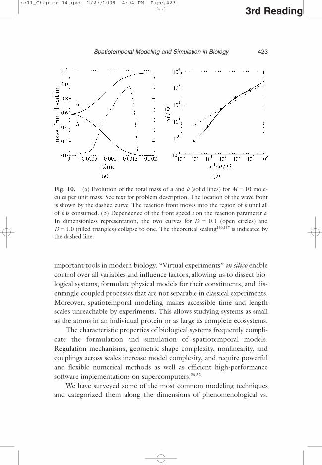
important tools in modern biology. “Virtual experiments” in silico enablecontrol over all variables and influence factors, allowing us to dissect bio-logical systems, formulate physical models for their constituents, and dis-entangle coupled processes that are not separable in classical experiments.Moreover, spatiotemporal modeling makes accessible time and lengthscales unreachable by experiments. This allows studying systems as smallas the atoms in an individual protein or as large as complete ecosystems.

The characteristic properties of biological systems frequently compli-cate the formulation and simulation of spatiotemporal models.Regulation mechanisms, geometric shape complexity, nonlinearity, andcouplings across scales increase model complexity, and require powerfuland flexible numerical methods as well as efficient high-performancesoftware implementations on supercomputers.26,32

We have surveyed some of the most common modeling techniquesand categorized them along the dimensions of phenomenological vs.


3rd Reading

Fig. 10. (a) Evolution of the total mass of a and b (solid lines) for M = 10 mole-cules per unit mass. See text for problem description. The location of the wave frontis shown by the dashed curve. The reaction front moves into the region of b until allof b is consumed. (b) Dependence of the front speed s on the reaction parameter c.In dimensionless representation, the two curves for D = 0.1 (open circles) andD = 1.0 (filled triangles) collapse to one. The theoretical scaling136,137 is indicated bythe dashed line.


physical, discrete vs. continuous, and deterministic vs. stochastic. Wesummarized for each of these model classes some of the available numer-ical simulation methods with pointers to specialized literature. We thenmotivated the use of point-based particle methods that do not requireany connectivity-based discretization and allow simulating both discreteand continuous systems. While their application to discrete systems isstandard, the use of continuum particle methods is less widespread. Wehave reviewed continuum particle methods in more detail and demon-strated their application to diffusion and reaction-diffusion problems.This was intended as an easy-to-follow introduction. Applications toother phenomena such as flows and waves are well documented in theliterature.

Notwithstanding the inherent complexity of biological systems, awealth of methods and tools are available that enable highly accurate andpredictive spatiotemporal simulations. At the same time, biology canserve as an important technology driver to stimulate the development ofnew methods and further advances in numerical analysis, computationalscience, and high-performance computing. Numerical methods that effi-ciently handle multi-scale systems27–31 and topological changes in com-plex geometries are at the forefront of research in computational science.In parallel, computer algorithms have to be efficient enough to deal withthe vast number of degrees of freedom, and software platforms must beavailable to effectively and robustly implement these algorithms onmulti-processor supercomputers.32 Just as fluid dynamics — in particular,the nonlinear, multi-scale problem of turbulence — has driven the devel-opment of numerical methods in the past, the major scientific goal ofmodeling an entire cell138 might continue to do so in the future.

References1. Turing AM. (1952) The chemical basis of morphogenesis. Phil Trans R Soc

Lond B 237: 37–72.2. Marée AFM. (2000) From Pattern Formation to Morphogenesis. PhD thesis.

University of Utrecht, Utrecht, The Netherlands.3. Harrison LG, Wehner S, Holloway DM. (2001) Complex morphogenesis of

surfaces: theory and experiment on coupling of reaction-diffusion patterningto growth. Faraday Discuss 120: 277–94.



4. Kaandorp JA, Sloot PMA, Merks RMH, et al. (2005) Morphogenesis of thebranching reef coral Madracis mirabilis. Proc R Soc Lond B Biol Sci272: 127–33.

5. Grant MR, Mostov KE, Tlsty TD, Hunt CA. (2006) Simulating properties ofin vitro epithelial cell morphogenesis. PLoS Comput Biol 2: e129.

6. Smith AE, Helenius A. (2004) How viruses enter animal cells. Science304: 237–42.

7. Dimitrov DS. (2004) Virus entry: molecular mechanisms and biomedicalapplications. Nat Rev Microbiol 2: 109–22.

8. Dinh AT, Theofanous T, Mitragotri S. (2005) A model for intracellulartrafficking of adenoviral vectors. Biophys J 89: 1574–88.

9. Greber UF, Way M. (2006) A superhighway to virus infection. Cell124: 741–54.

10. Marsh M, Helenius A. (2006) Virus entry: open sesame. Cell 124: 729–40.11. Marwan W. (2003) Theory of time-resolved complementation and its use to

explore the sporulation control network in Physarum polycephalum. Genetics164: 105–15.

12. Lipkow K, Andrews SS, Bray D. (2005) Simulated diffusion of phosphorylatedCheY through the cytoplasm of Escherichia coli. J Bacteriol 187: 45–53.

13. Dayel MJ, Hom EF, Verkman AS. (1999) Diffusion of green fluorescentprotein in the aqueous-phase lumen of the endoplasmic reticulum. Biophys J76: 2843–51.

14. Lippincott-Schwartz J, Snapp E, Kenworthy A. (2001) Studying proteindynamics in living cells. Nat Rev Mol Cell Biol 2: 444–56.

15. Verkman AS. (2002) Solute and macromolecule diffusion in cellular aqueouscompartments. Trends Biochem Sci 27: 27–33.

16. Alberts B, Bray D, Johnson A, et al. (1997) Essential Cell Biology. New York,NY: Garland Publication, Inc.

17. Rauch EM, Millonas MM. (2004) The role of trans-membrane signal trans-duction in Turing-type cellular pattern formation. J Theor Biol 226: 401–7.

18. Chaplain MAJ, Ganesh M, Graham IG. (2001) Spatio-temporal pattern for-mation on spherical surfaces: numerical simulation and application to solidtumour growth. J Math Biol 42: 387–423.

19. Jiang Y, Pjesivac-Grbovic J, Cantrell C, Freyer JP. (2005) A multiscale modelfor avascular tumor growth. Biophys J 89: 3884–94.

20. Macklin P, Lowengrub J. (2005) Evolving interfaces via gradients of geometry-dependent interior Poisson problems: application to tumor growth.J Comput Phys 203: 191–220.

21. Hense BA, Kuttler C, Müller J, et al. (2007) Does efficiency sensing unifydiffusion and quorum sensing? Nat Rev Microbiol 5: 230–9.

22. Müller J, Kuttler C, Hense BA, et al. (2006) Cell-cell communication byquorum sensing and dimension-reduction. J Math Biol 53: 672–702.



23. Slepchenko BM, Schaff JC, Carson JH, Loew LM. (2002) Computational cellbiology: spatiotemporal simulation of cellular events. Annu Rev Biophys BiomolStruct 31: 423–41.

24. Fall CP, Marland ES, Wagner JM, Tyson JJ. (2002) Computational Cell Biology.Interdisciplinary Applied Mathematics, Vol. 20. New York, NY: Springer.

25. Strogatz SH. (2000) Nonlinear Dynamics and Chaos. Boulder, CO: WestviewPress.

26. Takahashi K, Yugi K, Hashimoto K, et al. (2002) Computational challenges incell simulation: a software engineering approach. IEEE Intell Syst 17: 64–71.

27. Koumoutsakos P. (2005) Multiscale flow simulations using particles. AnnuRev Fluid Mech 37: 457–87.

28. Mielke A. (2006) Analysis, Modeling and Simulation of Multiscale Problems.Heidelberg, Germany: Springer.

29. Alt W, Chaplain M, Griebel M, Lenz J. (2008) Polymer and Cell Dynamics:Multiscale Modeling and Numerical Simulations. Basel, Switerland: Birkhäuser.

30. Kovalenko A, Gusarov S, Stepanova M. (2009) Multiscale Modeling: Concepts,Theories, and Applications. Boca Raton, Florida: CRC Press.

31. Chauviere A, Preziosi L, Verdier C. (2009) Cell Mechanics: From Single Scale-based Models to Multiscale Modeling. Boca Raton, Florida: Chapman & Hall.

32. Sbalzarini IF, Walther JH, Bergdorf M, et al. (2006) PPM — a highly efficientparallel particle-mesh library for the simulation of continuum systems.J Comput Phys 215: 566–88.

33. Reynwar BJ, Gregoria I, Harmandaris VA, et al. (2007) Aggregation and vesic-ulation of membrane proteins by curvaturemediated interactions. Nature447: 461–4.

34. Periole X, Huber T, Marrink SJ, Sakmar TP. (2007) G protein-coupled recep-tors self-assemble in dynamics simulations of model bilayers. J Am Chem Soc129: 10126–32.

35. Chu JW, Voth GA. (2006) Coarse-grained modeling of the actin filamentderived from atomistic-scale simulations. Biophys J 90: 1572–82.

36. Kashiwagi A, Urabe I, Kaneko K, Yomo T. (2006) Adaptive response of a genenetwork to environmental changes by fitness-induced attractor selection. PLoSONE 1: e49.

37. Burlando B. (1993) The fractal geometry of evolution. J Theor Biol163: 161–72.

38. Newman TJ, Antonovics J, Wilbur HM. (2002) Population dynamics with arefuge: fractal basins and the suppression of chaos. Theor Popul Biol 62: 121–8.

39. Grasman J, Brascamp JW, Van Leeuwen JL, Van Putten B. (2003) The multi-fractal structure of arterial trees. J Theor Biol 220: 75–82.

40. Smith TG Jr, Marks WB, Lang GD, et al. (1989) A fractal analysis of cellimages. J Neurosci Methods 27: 173–80.



41. Aon M, Cortassa S. (1994) On the fractal nature of cytoplasm. FEBS Lett344: 1–4.

42. Lahiri T, Chakrabarti A, Dasgupta AK. (1998) Multilamellar vesicular clusters ofphosphatidylcholine and their sensitivity to spectrin: a study by fractal analysis.J Struct Biol 123: 179–86.

43. Liebovitch LS, Scheurle D, Rusek M, Zochowski M. (2001) Fractal methodsto analyze ion channel kinetics. Methods 24: 359–75.

44. Li H, Li Y, Zhao H. (1990) Fractal analysis of protein chain conformation.Int J Biol Macromol 12: 6–8.

45. Li H, Chen S, Zhao H. (1991) Fat fractal and multifractals for protein andenzyme surfaces. Int J Biol Macromol 13: 210–6.

46. Saxton MJ. (1994) Anomalous diffusion due to obstacles: a Monte Carlostudy. Biophys J 66: 394–401.

47. Saxton MJ. (2001) Anomalous subdiffusion in fluorescence photobleachingrecovery: a Monte Carlo study. Biophys J 81: 2226–40.

48. Saxton MJ. (2007) A biological interpretation of transient anomalous subdif-fusion. I. Qualitative model. Biophys J 92: 1178–91.

49. Sbalzarini IF, Mezzacasa A, Helenius A, Koumoutsakos P. (2005) Effects oforganelle shape on fluorescence recovery after photobleaching. Biophys J89: 1482–92.

50. Frenkel D, Smit B. (2002) Understanding Molecular Simulation: FromAlgorithms to Applications. San Diego, CA: Academic Press.

51. Schrödinger E. (1948) What Is Life? The Physical Aspect of the Living Cell.Cambridge, UK: Cambridge University Press.

52. Marco E, Wedlich-Soldner R, Li R, et al. (2007) Endocytosis optimizes thedynamic localization of membrane proteins that regulate cortical polarity. Cell129: 411–22.

53. González-Segredo N. (2007) Amphiphilic fluids: mesoscopic modelling andcomputer simulations. In: Dillon KT (ed.), Soft Condensed Matter:New Research. New York, NY: Nova Science, pp. 125–56.

54. Farlow SJ. (1993) Partial Differential Equations for Scientists and Engineers.New York, NY: Dover Publications.

55. Strauss WA. (2007) Partial Differential Equations: An Introduction, 2nd ed.New York, NY: Wiley.

56. Øksendal BK. (2003) Stochastic Differential Equations, 6th ed. Berlin,Germany: Springer.

57. Manninen T, Linne ML, Ruohonen K. (2006) Developing Itô stochasticdifferential equation models for neuronal signal transduction pathways.Comput Biol Chem 30: 280–91.

58. Saarinen A, Linne ML, Yli-Harja O. (2008) Stochastic differential equationmodel for cerebellar granule cell excitability. PLoS Comput Biol 4: e1000004.



59. Alfonsi A, Cancès E, Turinici G, et al. (2005) Adaptive simulation of hybridstochastic and deterministic models for biochemical systems. In: Cancès E,Gerbeau JF (eds.). ESAIM: Proceedings, Vol. 14, pp. 1–13.

60. Salis H, Sotiropoulos V, Kaznessis YN. (2006) Multiscale Hy3S: hybridstochastic simulation for supercomputers. BMC Bioinformatics 7: 93–112.

61. Gillespie DT. (1976) A general method for numerically simulating thestochastic time evolution of coupled chemical reactions. J Comput Phys22: 403–34.

62. Gillespie DT. (1977) Exact stochastic simulation of coupled chemical reac-tions. J Phys Chem 81: 2340–61.

63. Gibson MA, Bruck J. (2000) Efficient exact stochastic simulation of chemicalsystems with many species and many channels. J Phys Chem A 104: 1876–89.

64. Stundzia A, Lumsden C. (1996) Stochastic simulation of coupled reaction-diffusion processes. J Comput Phys 127: 196–207.

65. Isaacson SA, Peskin CS. (2006) Incorporating diffusion in complex geometriesinto stochastic chemical kinetics simulations. SIAM J Sci Comput 28: 47–74.

66. Liu JS. (2001) Monte Carlo Strategies in Scientific Computing. Springer Seriesin Statistics. New York, NY: Springer.

67. Rubinstein RY, Kroese DP. (2007) Simulation and the Monte Carlo Method,2nd ed. New York, NY: Wiley.

68. Milizzano F, Saffman PG. (1977) The calculation of large Reynolds numbertwo-dimensional flow using discrete vortices with random walk. J Comput Phys23: 380–92.

69. Schweitzer F. (2003) Brownian Agents and Active Particles. On the Emergenceof Complex Behavior in the Natural and Social Sciences. Springer Series inSynergetics. Berlin, Germany, Springer.

70. Gaylord RJ, Nishidate K. (1996) Modeling Nature: Cellular AutomataSimulations with Mathematica. New York, NY: Springer.

71. Ilachinski A. (2001) Cellular Automata. Singapore: World ScientificPublishing.

72. Schiff JL. (2007) Cellular Automata: A Discrete View of the World. Wiley Seriesin Discrete Mathematics and Optimization. Hoboken, NJ: Wiley Interscience.

73. Terano T, Kita H, Kaneda T, et al. (2005) Agent-based Simulation: FromModeling Methodologies to Real-World Applications. Tokyo, Japan: Springer.

74. Mosler HJ, Schwarz K, Ammann F, Gutscher H. (2001) Computer simulationas a method of further developing a theory: simulating the elaboration likeli-hood model (ELM). Pers Soc Psychol Rev 5: 201–15.

75. Kloeden PE, Platen E. (1992) Numerical Solution of Stochastic DifferentialEquations. Stochastic Modeling and Applied Probability. Berlin, Germany:Springer.

76. Higham DJ. (2001) An algorithmic introduction to numerical simulation ofstochastic differential equations. SIAM Rev 43: 525–46.



77. Evans G, Blackledge J, Yardley P. (1999) Numerical Methods for PartialDifferential Equations. Berlin, Germany: Springer.

78. Grossmann C, Roos HG, Stynes M. (2007) Numerical Treatment of PartialDifferential Equations. Berlin, Germany: Springer.

79. Smith GD. (1985) Numerical Solution of Partial Differential Equations: FiniteDifference Methods, 3rd ed. Oxford, UK: Clarendon Press.

80. Reddy JN. (1993) An Introduction to the Finite Element Method, 2nd ed.New York, NY: McGraw-Hill.

81. Zienkiewicz OC, Taylor RL. (2005) The Finite Element Method, 6th ed.Oxford, UK: Butterworth-Heinemann.

82. Benkhaldoun F, Vilsmeier R. (1999) Finite Volumes for Complex Applications,Vols. 1 and 2. Paris, France: Hermes Science Publications.

83. LeVeque RJ. (2002) Finite Volume Methods for Hyperbolic Problems.Cambridge, UK: Cambridge University Press.

84. Kincaid DR, Cheney EW. (2001) Numerical Analysis: Mathematics of ScientificComputing, 3rd ed. Pacific Grove, CA: Brooks/Cole.

85. Cottet GH, Koumoutsakos P. (2000) Vortex Methods — Theory and Practice.New York, NY: Cambridge University Press.

86. Li S, Liu WK. (2004) Meshfree Particle Methods. Berlin, Germany: Springer.87. Liu GR, Gu YT. (2005) An Introduction to Meshfree Methods and Their

Programming. Berlin, Germany: Springer.88. de Berg M, van Krefeld M, Overmars M, Schwarzkopf O. (2000)

Computational Geometry: Algorithms and Applications, 2nd ed. Heidelberg,Germany: Springer.

89. Schumaker LL. (1987) Triangulation methods. In: Chui CK, Schumaker LL,Utreras FI (eds.). Topics in Multivariate Approximation. New York, NY:Academic Press, pp. 219–32.

90. Bänsch E, Morin P, Nochetto RH. (2005) A finite element method for surfacediffusion: the parametric case. J Comput Phys 203: 321–43.

91. Novak IL, Gao F, Choi YS, et al. (2007) Diffusion on a curved surface coupled todiffusion in the volume: application to cell biology. J Comput Phys 226: 1271–90.

92. Haber J, Zeilfelder F, Davydov O, Seidel HP. (2001) Smooth approximationand rendering of large scattered data sets. In: Proc IEEE Visualization,pp. 341–7.

93. Sethian JA. (1999) Level Set Methods and Fast Marching Methods. Cambridge,UK: Cambridge University Press.

94. Enright D, Fedkiw R, Ferziger J, Mitchell I. (2002) A hybrid particle level setmethod for improved interface capturing. J Comput Phys 183: 83–116.

95. Hieber SE, Koumoutsakos P. (2005) A Lagrangian particle level set method.J Comput Phys 210: 342–67.

96. Sbalzarini IF, Hayer A, Helenius A, Koumoutsakos P. (2006) Simulations of(an)isotropic diffusion on curved biological surfaces. Biophys J 90: 878–85.



97. Ahusborde E, Gruber R, Azaiez M, Sawley ML. (2007) Physics-conformingconstraints-oriented numerical method. Phys Rev E Stat Nonlin Soft MatterPhys 75: 056704.

98. Courant R, Friedrichs K, Lewy H. (1928) Über die partiellen Differenzenglei-chungen der mathematischen Physik. Math Ann 100: 32–74.

99. Courant R, Friedrichs K, Lewy H. (1967) On the partial difference equationsof mathematical physics. IBM Res Dev 11: 215–34.

100. Bergdorf M, Koumoutsakos P. (2006) A Lagrangian particle-wavelet method.Multiscale Model Simul 5: 980–95.

101. Bergdorf M, Cottet GH, Koumoutsakos P. (2005) Multilevel adaptive particlemethods for convection-diffusion equations. Multiscale Model Simul4: 328–57.

102. Haber S. (1967) Midpoint quadrature formulas. Math Comput 21: 719–21.103. Degond P, Mas-Gallic S. (1989) The weighted particle method for convection-

diffusion equations. Part 1: the case of an isotropic viscosity. Math Comput53: 485–507.

104. Degond P, Mas-Gallic S. (1989) The weighted particle method for convection-diffusion equations. Part 2: the anisotropic case. Math Comput 53: 509–25.

105. Eldredge JD, Leonard A, Colonius T. (2002) A general deterministic treat-ment of derivatives in particle methods. J Comput Phys 180: 686–709.

106. Harlow FH. (1964) Particle-in-cell computing method for fluid dynamics.Methods Comput Phys 3: 319–43.

107. Hockney RW, Eastwood JW. (1988) Computer Simulation Using Particles.Bristol, UK: Institute of Physics Publishing.

108. Trottenberg U, Oosterlee C, Schueller A. (2001) Multigrid. San Diego, CA:Academic Press.

109. Monaghan JJ. (1985) Extrapolating B splines for interpolation. J Comput Phys60: 253–62.

110. Greengard L, Rokhlin V. (1988) The rapid evaluation of potential fields in threedimensions. In: Anderson C, Greengard C (eds.). Vortex Methods. Lecture Notesin Mathematics, Vol. 136. Berlin, Germany: Springer-Verlag, pp. 121–41.

111. Verlet L. (1967) Computer experiments on classical fluids. I. Thermodynamicalproperties of Lennard-Jones molecules. Phys Rev 159: 98–103.

112. Sutmann G, Stegailov V. (2006) Optimization of neighbor list techniques inliquid matter simulations. J Mol Liq 125: 197–203.

113. Barnes J, Hut P. (1986) A hierarchical O(NlogN) force-calculation algorithm.Nature 324: 446–9.

114. Greengard L, Rokhlin V. (1987) A fast algorithm for particle simulations.J Comput Phys 73: 325–48.

115. Cheng H, Greengard L, Rokhlin V. (1999) A fast adaptive multipole algorithmin three dimensions. J Comput Phys 155: 468–98.



116. Berg H. (1993) Random Walks in Biology. Princeton, NJ: Princeton UniversityPress.

117. Brown R. (1828) A brief account of microscopical observations made in themonths of June, July, and August, 1827, on the particles contained in thepollen of plants; and on the general existence of active molecules in organic andinorganic bodies. Philos Mag 4: 161–73.

118. Einstein A. (1905) Über die von der molekularkinetischen Theorie der Wärmegeforderte Bewegung von in ruhenden Flüssigkeiten suspendierten Teilchen.Ann Phys 17: 549–60.

119. Nadler SB Jr. (1992) Continuum Theory. Basel, Switzerland: M. Dekker.120. Chorin AJ. (1973) Numerical study of slightly viscous flow. J Fluid Mech

57: 785–96.121. Chandrasekhar S. (1943) Stochastic problems in physics and astronomy.

Rev Mod Phys 15: 1–89.122. Van Kampen NG. (2001) Stochastic Processes in Physics and Chemistry, 2nd ed.

Amsterdam, The Netherlands: North Holland.123. Koumoutsakos P, Leonard A, Pépin F. (1994) Boundary conditions for viscous

vortex methods. J Comput Phys 113: 52–61.124. Fisher RA. (1937) The advance of advantageous genes. Ann Eugen 7: 335–69.125. Kolmogorov AN, Petrovsky IG, Piskunov NS. (1937) Étude de l’équation de

la diffusion avec croissance de la quantité de matière et son application à unproblème biologique. Bull Univ d’Etat Moscou (Bjul Moskowskogo Gos Univ),Sér Int A 1: 1–26.

126. Riordan J, Doering CR, ben Avraham D. (1995) Fluctuations and stability ofFisher waves. Phys Rev Lett 75: 565–8.

127. Gierer A, Meinhardt H. (1972) A theory of biological pattern formation.Kybernetik 12: 30–9.

128. Turk G. (1991) Generating textures on arbitrary surfaces using reaction-diffusion. Comput Graph 25: 289–98.

129. Madzvamuse A, Wathen AJ, Maini PK. (2003) A moving grid finite elementmethod applied to a model biological pattern generator. J Comput Phys190: 478–500.

130. Grimm HP, Verkhovsky AB, Mogilner A, Meister JJ. (2003) Analysis of actindynamics at the leading edge of crawling cells: implications for the shape ofkeratocyte lamellipodia. Eur Biophys J 32: 563–77.

131. Plimpton SJ, Slepoy A. (2005) Microbial cell modeling via reacting diffusiveparticles. J Phys Conf Ser 16: 305–9.

132. Miura T, Maini PK. (2004) Speed of pattern appearance in reaction-diffusionmodels: implications in the pattern formation of limb bud mesenchyme cells.Bull Math Biol 66: 627–49.

133. Bhalla US. (2004) Models of cell signaling pathways. Curr Opin Genet Dev14: 375–81.



134. Bray D, Bourret RB, Simon MI. (1993) Computer simulation of the phos-phorylation cascade controlling bacterial chemotaxis. Mol Biol Cell 4: 469–82.

135. Jönsson H, Heisler M, Reddy GV, et al. (2005) Modeling the organization ofthe WUSCHEL expression domain in the shoot apical meristem.Bioinformatics 21: i232–40.

136. Benguria RD, Depassier MC. (1996) Speed of fronts of the reaction-diffusionequation. Phys Rev Lett 77: 1171–3.

137. Berestycki H, Hamel F, Nadirashvili N. (2005) The speed of propagation forKPP type problems. I: periodic framework. J Eur Math Soc 7: 173–213.

138. The 2020 Science Group. (2005) Towards 2020 Science. Cambridge, UK:Microsoft Research Cambridge.



MODELLING OF BIOLOGICAL SYSTEMS - MPI-CBG · method. One often hears that this is because...

Documents

Transcript of MODELLING OF BIOLOGICAL SYSTEMS - MPI-CBG · method. One often hears that this is because...