NO3

-Flagellates Mesozooplankton

Bacteria

Detritus

Diatoms MicrozooplanktonNH4

+

EUR 22952 EN - 2007

Modelling mesocosm experiments

Sibylle Dueri, Dimitar Marinov, José-Manuel Zaldívar, Morten Hjorth and Ingela Dahllöf

2

The mission of the Institute for Environment and Sustainability is to provide scientific-technical support to the European Union’s Policies for the protection and sustainable development of the European and global environment. European Commission Joint Research Centre Contact information Address: Via E. Fermi 1, TP 272 E-mail: jose.zaldivar-comenges@jrc.it Tel.: +39-0332-789202 Fax: +39-0332-785807 http://www.jrc.ec.europa.eu Legal Notice Neither the European Commission nor any person acting on behalf of the Commission is responsible for the use which might be made of this publication. A great deal of additional information on the European Union is available on the Internet. It can be accessed through the Europa server http://europa.eu/ JRC 40018 EUR 22952 EN

ISBN 978-92-79-07402-8

ISSN 1018-5593

DOI: 10.2788/3592

Luxembourg: Office for Official Publications of the European Communities © European Communities, 2007 Reproduction is authorised provided the source is acknowledged Printed in Italy

3

Table of Contents

1. INTRODUCTION .................................................................................................................. 5

2. MESOCOSM EXPERIMENTS............................................................................................. 6

3. FOOD WEB MODEL ............................................................................................................ 7

3.1. PHYTOPLANKTON ................................................................................................................. 8

3.2. ZOOPLANKTON..................................................................................................................... 9

3.3. BACTERIA ............................................................................................................................ 9

3.4. DETRITUS........................................................................................................................... 10

3.5. TOXIC EFFECT OF CONTAMINANT ........................................................................................ 10

3.6. PARAMETERS, INITIAL CONDITIONS AND METEREOLOGICAL FORCING OF THE MESOCOSM

EXPERIMENT SIMULATION ........................................................................................................... 10

4. RESULTS ............................................................................................................................. 12

4.1. WATER TEMPERATURE....................................................................................................... 12

4.2. CONTROL AND ENRICHED MESOCOSM.................................................................................. 12

4.3. PYRENE DEGRADATION....................................................................................................... 15

4.4. TOXIC EFFECTS OF PYRENE IN THE MESOCOSM..................................................................... 16

5. DISCUSSION ....................................................................................................................... 19

6. CONCLUSIONS................................................................................................................... 19

7. REFERENCES ..................................................................................................................... 21

4

List of Tables

Table 3.1: Parameters used for the simulation of the mesocosm experiment 11

Table 4.1: Parameters for the Pyrene dose-response function in the model. 18

List of Figures Figure 3.1. Simplified flow diagram in the marine ecosystem. 7

Figure 3.2. Sun radiation and temperature forcing used for the simulations. 12

Figure 4.1. Simulated surface water temperature fluctuations during the mesocosm experiment. 13

Figure 4.2. Observed nitrate and ammonia concentration in the control (blue) and enriched (green) mesocosm,

used as forcing). 14

Figure 4.3. Comparison of the simulated values (line) with the observed values (points) for the control

mesocosm. 15

Figure 4.4. Comparison of the simulated values (line) with the observed values (points) for the enriched

mesocosm. 15

Figure 4.5. Simulation of the biomass and detritus distribution in the food web for the control mesocosm. 16

Figure 4.6. Simulation of the biomass and detritus distribution in the food web for the enriched mesocosm 16

Figure 4.7. Observed (cross) and simulated (line) concentration of pyrene in the mesocosm. 17

Figure 4.8. Dose-response curves used in the model. Dotted line represents the concentration of pyrene after

addition. 18

Figure 4.9. Comparison of the simulated values (line) with the observed values (points) for the mesocosm with

pyrene addition. 19

Figure 4.10. Comparison of the simulated values (line) with the observed values (points) for the enriched

mesocosm with pyrene addition. 19

Figure 4.11. Simulation of the biomass and detritus distribution in the mesocosm with pyrene addition. 20

Figure 4.12. Simulation of the biomass and detritus distribution for the enriched mesocosm with pyrene

addition. 21

5

1. Introduction

During the last decades coastal waters have been exposed to an increasing pressure of nutrients and

contaminants related to agricultural, industrial and domestic activities. Input from rivers and effluents

are one of the major sources of pollution in the coastal area from, but also inputs from atmospheric

transport (dry and wet deposition and air-water exchange) can be a major contributor. Normally, a

mixture of contaminants is present in transitional, coastal as well as marine waters, affecting their

ecosystems.

The assessment of the combined effect of eutrophication and pollution on ecosystems is not

straightforward due to complex interactions and feedbacks. Eutrophication may increase the primary

production, dilute the contaminant in the biomass and furthermore increase the scavenging with the

organic matter (Koelmans et al. 2001). On the other hand contaminants can have direct and indirect

effects on the ecosystem balance and the growth of populations (Fleeger et al. 2003). Direct effects are

caused by the toxicity of contaminants, which increase the mortality of the affected population;

conversely indirect effects are the consequence of reduced food availability or reduced grazing. Thus,

while nutrient acts on the bottom level of the food chain, contaminants may affect higher trophic levels

and the correct understanding of the relative importance of top-down versus bottom-up controls is

essential to evaluate the system.

The traditional approach for the modeling of contaminants in the water column is to consider two well-

mixed boxes during stratification periods and one well-mixed the rest of the time (Schwarzenbach et

al., 2003; Meijer et al., 2006). The extensive number of 0D models for hydrophobic organic

compounds (Wania and Mackay, 1996; Scheringer et al., 2000; Dalla Valle et al., 2003; Dueri et al.,

2005) contrasts with the lack of spatially and temporally resolved models, with the exception of the

recently developed coastal lagoon model for herbicides (Carafa et al., 2006) and the one for HCH by

Ilyina et al. (2006). A 1D dynamic hydrodynamic-contaminant model has been developed to analyze

the influence of vertical mixing on the distribution of POPs in the water column (Jurado et al., 2007;

Marinov et al., 2007). The model was applied to the organic contaminants families selected in

Thresholds, i.e. PCBs, PAHs, and PBDEs, plus dioxins and furans, PCDD/Fs and details are presented

in the Deliverable 2.6.2. Recently this 1D dynamic hydrodynamic-contaminant model was coupled

with a food-web ecological model that considers phytoplankton, zooplankton, bacteria and detritus

(Deliverable 2.6.3). The newly developed model uses nutrient concentrations as forcing and considers

the bioaccumulation of POPs in all the ecological compartments. A first validation of the coupled

model has been achieved using experimental data on PAHs obtained at the Finokalia Station, Island of

Crete, Greece (Tsapakis et al., 2005 and 2006). The results showed that the model is able to reproduce

the experimental concentrations as well as the measured fluxes. However, due to the low

6

concentrations of PAHs in the considered remote area environment, the toxic effect model could not be

validated with those data.

Within the framework of the Threshold project, mesocosm experiments have been carried out in the

Isefjord (Denmark) by NERI (Deliverable 4.3.3) to elucidate the combined effects of nutrient and

pyrene on an ecosystem composed of phytoplankton, zooplankton and bacteria (Hjorth et al. 2007).

The experimental results are used here to validate the model presented in Deliverable 2.6.3 on a

smaller scale, including the toxic effect model and at the same time investigate the direct and indirect

effects observed in the system.

2. Mesocosm experiments

A detailed description of the experimental work and its results is reported in Deliverable 4.3.3. The

mesocosm experiments were carried out in the Isefjord (N: 55 42 44.4, E 11 47 28.51) between 23rd

April and 4th

May. The average depth of the fjord is 5-7 m. Twelve clear polyethylene cylindrical

enclosures were filled with 3 m3 ambient water and were attached 200 m from the shore. The bags

were 2.5 m deep, and with a diameter of 1.25 m. The average temperature of measured in the bags

during the experiments was between 10-15 ºC and the salinity was constant at 16 ppt. Sedimentation

was avoided by gently pumping water from the bottom of the bags. Four different experiments were

carried out:

1. Control experiment without any addition of nutrient or contaminant;

2. Enriched experiment with nutrient addition on day -1 and day 6; concentrations after addition: 4.8

µmol/L ammonia (NH3Cl), 9.6 µmol/L silicate (Na2SiO3), 0.3 µmol/L phosphate (NaH2PO4)

and ratio of 16:32:1 (N:Si:P);

3. Contaminant experiment with Pyrene addition (50nmol/L) on day 0 and day 7;

4. Experiment with contaminant and nutrient addition.

During the experiment different parameters were monitored: Chl a [µg/L], concentration of nutrients

(Si, 34−

PO PO4, +4NH , −− + 23 NONO ) [µmol/L], primary production [dpm], bacterial activity [dpm]

and copepod abundance [ind/L]. Also the distribution of 3 different communities of phytoplankton (2

flagellates and 1 diatom) was recorded by means of pigment analysis.

In addition to the experiments on the combined effect of nutrient and contaminants, another set of

mesocosm experiments were carried out simultaneously in the Isefjord to observe the dynamics of

attached microbial communities in an enriched system (Tang et al. 2006). Results from this study,

which characterizes in detail the bacterial community and the zooplankton communities, were used to

fit the bacterial part of the food web model and set the initial conditions of the micro- and

mesozooplankton families.

7

3. Food web model

In order to simulate the toxic effects of contaminants in marine ecosystems as well as the effects of the

biological pump on the dynamics of contaminants a simplified model has been developed. This model

was considered as the minimum model able to deal with effects observed in the mesocosm

experiments carried out by NERI (D.4.3.3). Deliverable D 2.6.3 describes the model’s capabilities and

features as well as the validation of the model using data of the Mediterranean Cruise and other

campaigns. Hereafter we will summarize the main characteristics of the model.

The main compartments and interactions integrated in the model are represented in Fig. 3.1. The

phytoplankton compartment is subdivided in two groups, diatoms and flagellates (Pd, Pf). Similarly,

zooplankton has also been split into two groups representing microzooplankton (< 200 µm) and

mesozooplankton (0.2-2 mm) (Zs, Zl). Moreover the microbial loop which accounts for the

mineralization of dead organic matter, called detritus (D), performed by the bacteria (B), is

incorporated in the model.

NO3

-Flagellates Mesozooplankton

Bacteria

Detritus

Diatoms MicrozooplanktonNH4

+

Figure 3.1. Simplified flow diagram in the marine ecosystem.

Nitrate and ammonium concentration in the water column are considered as forcing and therefore there

is no dynamic interaction between the nutrient and the food web. The ordinary differential equations

may be written as:

PdmZlgrazingZsgrazingPdgrowthdt

dPdPd

Zl

Pd

Zs

PdPd ⋅−⋅−⋅−⋅= (1)

PfmZlgrazingZsgrazingPfgrowthdt

dPfPf

Zl

Pf

Zs

PfPf ⋅−⋅−⋅−⋅= (2)

( )2

ZsmZsexcre

ZlgrazingZseffgrazingZseffgrazinggrazingdt

dZs

ZsZs

Zl

ZsB

Zs

BP

Zs

Pf

Zs

Pd

⋅−⋅−

⋅−⋅⋅+⋅⋅+= (3)

8

( )2

ZlmZlexcre

ZleffgrazingZleffgrazinggrazingdt

dZl

ZlZl

Zs

Zl

ZsP

Zl

Pf

Zl

Pd

⋅−⋅−

⋅⋅+⋅⋅+= (4)

ZsgrazingBkdBgrowthdt

dB Zs

BBB ⋅−⋅−⋅= (5)

DwDuptunassimunassimunassimmortdt

dDsB

BZP ⋅−⋅−−+++= βdetdetdetdet (6)

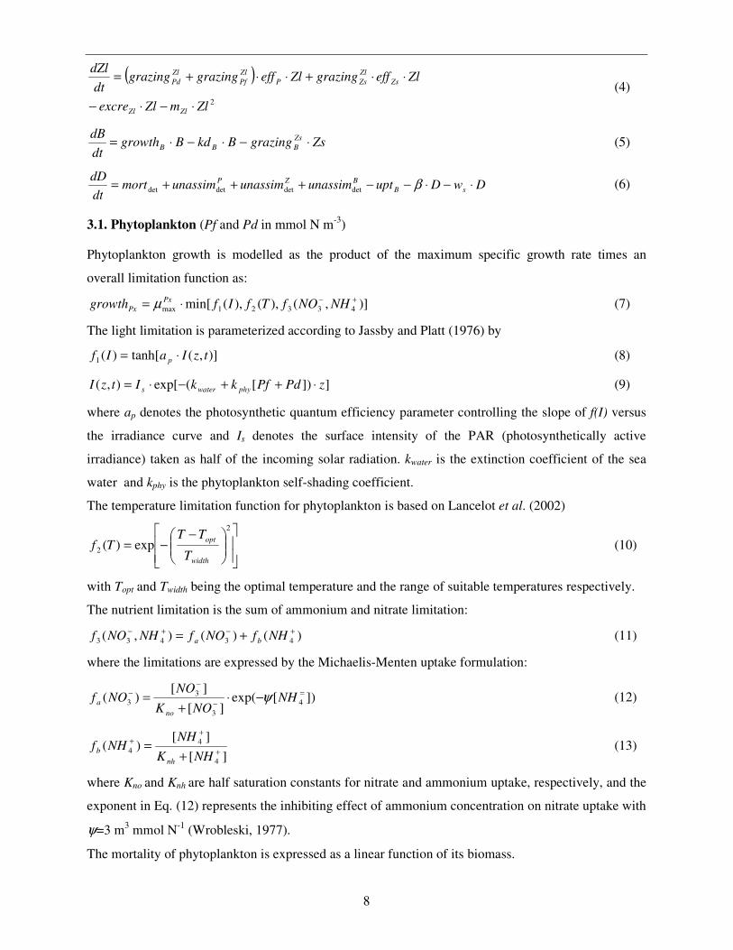
3.1. Phytoplankton (Pf and Pd in mmol N m-3

)

Phytoplankton growth is modelled as the product of the maximum specific growth rate times an

overall limitation function as:

)],(),(),(min[ 43321max

+−⋅= NHNOfTfIfgrowthPx

Px µ (7)

The light limitation is parameterized according to Jassby and Platt (1976) by

)],(tanh[)(1 tzIaIf p ⋅= (8)

]])[(exp[),( zPdPfkkItzI phywaters ⋅++−⋅= (9)

where ap denotes the photosynthetic quantum efficiency parameter controlling the slope of f(I) versus

the irradiance curve and Is denotes the surface intensity of the PAR (photosynthetically active

irradiance) taken as half of the incoming solar radiation. kwater is the extinction coefficient of the sea

water and kphy is the phytoplankton self-shading coefficient.

The temperature limitation function for phytoplankton is based on Lancelot et al. (2002)

−−=

2

2 exp)(width

opt

T

TTTf (10)

with Topt and Twidth being the optimal temperature and the range of suitable temperatures respectively.

The nutrient limitation is the sum of ammonium and nitrate limitation:

)()(),( 43433

+−+− += NHfNOfNHNOf ba (11)

where the limitations are expressed by the Michaelis-Menten uptake formulation:

])[exp(][

][)( 4

3

33

=

−

−− −⋅

+= NH

NOK

NONOf

no

a ψ (12)

][

][)(

4

44 +

++

+=

NHK

NHNHf

nh

b (13)

where Kno and Knh are half saturation constants for nitrate and ammonium uptake, respectively, and the

exponent in Eq. (12) represents the inhibiting effect of ammonium concentration on nitrate uptake with

ψ=3 m3 mmol N

-1 (Wrobleski, 1977).

The mortality of phytoplankton is expressed as a linear function of its biomass.

9

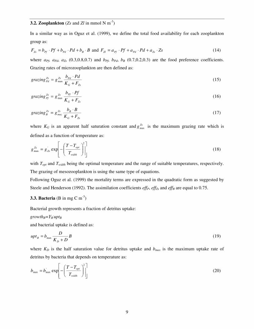
3.2. Zooplankton (Zs and Zl in mmol N m-3

)

In a similar way as in Oguz et al. (1999), we define the total food availability for each zooplankton

group as:

BbPdbPfbF BPdPfZs ⋅+⋅+⋅= and ZsaPdaPfaF ZsPdPfZl ⋅+⋅+⋅= (14)

where aPf, aPd, aZs (0.3,0.8,0.7) and bPf, bPd, bB (0.7,0.2,0.3) are the food preference coefficients.

Grazing rates of microzooplankton are then defined as:

ZsG

PdZsZs

PdFK

Pdbggrazing

+

⋅= max (15)

ZsG

PfZsZs

PfFK

Pfbggrazing

+

⋅= max (16)

ZsG

BZs

maz

Zs

BFK

Bbggrazing

+

⋅= (17)

where KG is an apparent half saturation constant and Zsgmax

is the maximum grazing rate which is

defined as a function of temperature as:

−−=

2

'

max expwidth

opt

Zs

Zs

T

TTgg (18)

with Topt and Twidth being the optimal temperature and the range of suitable temperatures, respectively.

The grazing of mesozooplankton is using the same type of equations.

Following Oguz et al. (1999) the mortality terms are expressed in the quadratic form as suggested by

Steele and Henderson (1992). The assimilation coefficients effP, effZs and effB are equal to 0.75.

3.3. Bacteria (B in mg C m-3

)

Bacterial growth represents a fraction of detritus uptake:

growthB=YB.uptB

and bacterial uptake is defined as:

BDK

Dbupt

D

B+

= max (19)

where KD is the half saturation value for detritus uptake and bmax is the maximum uptake rate of

detritus by bacteria that depends on temperature as:

−−=

2

'maxmax exp

width

opt

T

TTbb (20)

10

3.4. Detritus (D in mg C m-3

)

Phytoplankton, zooplankton and bacteria mortalities plus fecal pellets, constitute the unassimilated part

of ingested food, contribute to the detritus compartment. Detritus due to mortality is expressed as:

( ) ( ) BkdCNZlmZsmCNPfmPdmmort BZZlZsPPfPd ⋅+⋅⋅+⋅+⋅⋅+⋅= 22

det (21)

where CNP and CNZ are ratios of mg C/mmol N for phytoplankton and zooplankton, respectively.

CNP=48, CNZ =63. The other component consists on the unassimilated part of ingested food by

zooplankton, that can be written as:

P

Zl

Pf

Zl

PdPP

Zs

Pf

Zs

Pdp

PCNZlgrazinggrazingeffCNZsgrazinggrazingeffunassim ⋅⋅+⋅−+⋅⋅+⋅−= )()1()()1(det

(22)

Z

Zl

ZsZ

ZCNZlgrazingeffunassim ⋅⋅⋅−= )1(det (23)

B

Zs

BB

BCNZsgrazingeffunassim ⋅⋅⋅−= )1(det (24)

where CNB is the ratio of mg C/mmol N for bacteria, CNB=48. The other two terms in the mass balance

for detritus account for the mineralization and for the settling, with a detritus decomposition rate

β=4.17 10-3

h-1

and a sinking velocity ws=8.33 10-2

m h-1

.

3.5. Toxic effect of contaminant

In the model the dose-response effects have been simulated using the Weibull equation:

)]logexp(exp[1)( 1021 xxf θθ +−−= (25)

The mortality of the ecological compartments is changed as a function of the concentration of

contaminant by adding to the mortality rate in the original equations, Eqs. (1)-(5), the induced pyrene

mortality as given by Eq. (25). In addition this mortality term produces an increase in the detritus

fraction and therefore a change in the distribution of the contaminant between dissolved and particulate

phases.

3.6. Parameters, initial conditions and meteorological forcing of the mesocosm experiment

simulation

The parameters of the food web model that have been used for the simulation of the mesocosm

experiment are summarized in Table 3.1.

Initial concentration of phytoplankton was calculated from the Chl a concentration reported by in D

4.3.3 for the mesocosm experiment. Total concentration was partitioned between diatoms and

flagellates according to the proportion observed in the system. Therefore in the simulation of the

control experiment the initial concentration was set to 5 and 2.5 mmol N m-3

for the flagellates and the

diatoms, respectively. Alternatively, in the enriched experiment they were set to 10 mmol N m-3

and 5

mmol N m-3

, respectively. The initial concentration of the large zooplankton compartment was defined

according to the abundance of copepods at the beginning of the experiment, 3.5 ind L-1

. Taking a

11

mean carbon content per copepod of 2.5 µg C ind-1

(Van Nieuwerburgh et al. 2005) and converting to

nitrogen the initial concentration of copepods corresponds to 0.14 mmol N m-3

. According to Tang et

al. (2006), rotifers are the most abundant microzooplankton population and their mean abundance

during the experiment was 106.3 ind L-1

. Taking a conversion coefficient of 0.6 µg C ind-1

(White

and Roman 1992, Straile 1997) we obtain a mean concentration of rotifer of 1 mmol N m-3

. The initial

value was set to half the mean value, corresponding to 0.5 mmol N m-3

. The initial concentration of

bacteria was set to 10 mg C m-3

corresponding to the value measured at the beginning of the mesocosm

experiment by Tang et al. 2006. Since data about the detritus concentration in the Isefjord is missing, it

was estimated from the particulate organic carbon POC concentration measured in the Gullmar Fjord

and Stretudden (Erlandsson et al. 2006) and was set to 200 mg C m-3

.

Table 3.1: Parameters used for the simulation of the mesocosm experiment.

Parameter Definition Value Unit

ap Photosynthetis efficiency 0.01 m2 W-1

kwater Light extiction coefficient in sea water (coastal) 0.30 m-1

kphy Phytoplankton self shading coefficient 0.08 mmol N-1

µmax Pd Maximum growht rate for diatoms 0.03 h-1

µmax Pf Maximum growht rate for flagellates 0.03 h-1

Topt, Pd Optimal temperature for diatoms 10 ºC

Topt, Pf Optimal temperature for flagellates 15 ºC

Twidth, Pd Range of temperatures for diatoms 10 ºC

Twidth, Pf Range of temperatures for flagellates 10 ºC

Kno Half saturation for nitrate uptake 2 mmol N m3

Knh Half saturation for ammonium uptake 1 mmol N m3

ψ Ammonium inhibition parameter 3 m3 mmol N

-1

mPd Diatoms mortality rate 0.0025 h-1

mPf Flagellates mortality rate 0.0025 h-1

gZs’ Microzooplankton max grazing rate 0.050 h-1

gZl’ Mesozooplankton max grazing rate 0.045 h-1

Topt, Zs Optimal temperature for microzooplankton 14 ºC

Topt, Zl Optimal temperature for mesozooplankton 14 ºC

Twidth, Zs Range of temperature for microzooplankton 9 ºC

Twidth, Zl Range of temperature for mesozooplankton 9 ºC

KG Half saturation for zooplankton grazing 1.5 mmol N m-3

mZs Microzooplankton mortality rate 0.0022 h-1

mZl Mesozooplankton mortality rate 0.0024 h-1

b'max Maximum uptake of detritus by bacteria 0.4 h-1

KD Half saturation for detritus uptake by bacteria 25 mg C m-3

Topt,B Optimal temperature for bacteria 30 ºC

Twidth,B Range of temperature for bacteria 18 ºC

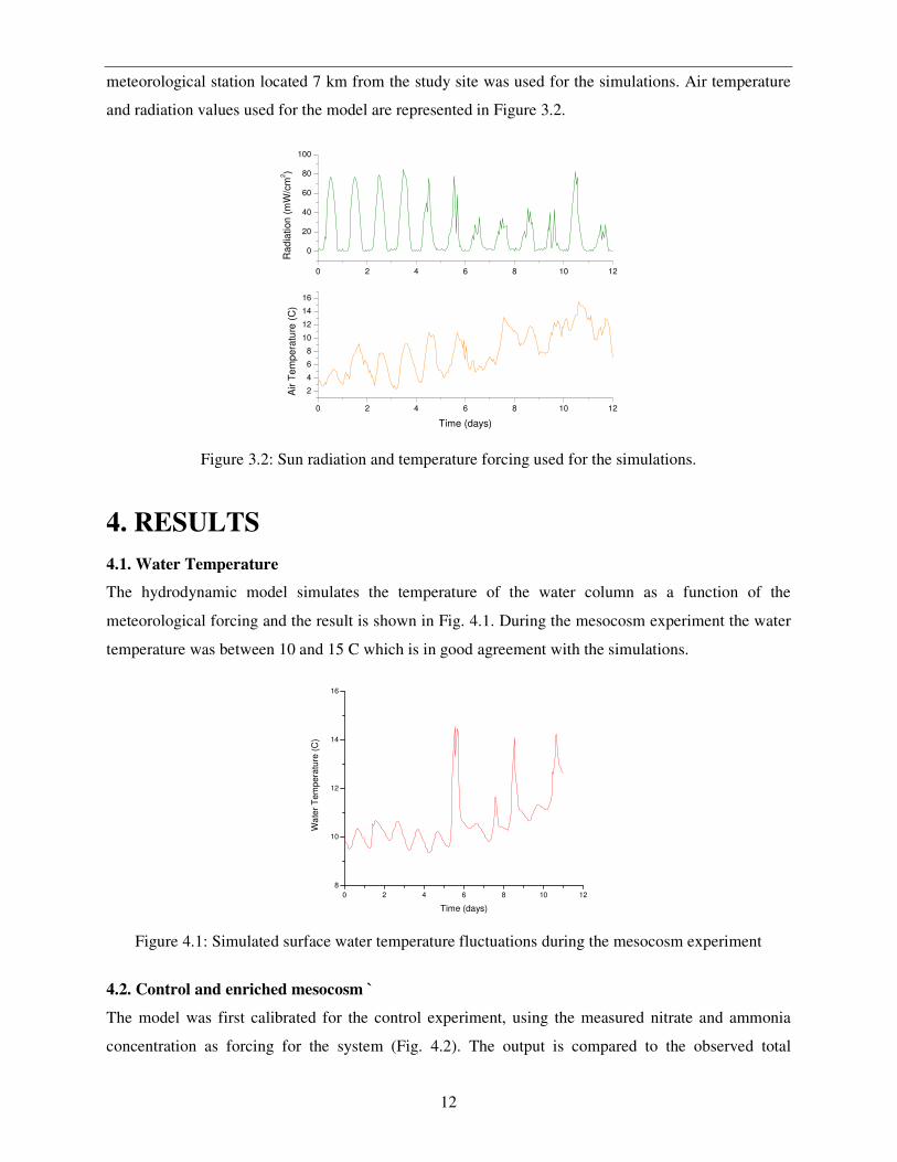
The model also requires meteorological data for wind (speed and direction), humidity, cloud coverage,

temperature and rainfall. The meteorological forcing is very important for the food web model, since

primary production is highly influenced by temperature and radiation conditions. Data from a

12

meteorological station located 7 km from the study site was used for the simulations. Air temperature

and radiation values used for the model are represented in Figure 3.2.

0 2 4 6 8 10 12

2

4

6

8

10

12

14

16A

ir T

em

pe

ratu

re (

C)

Time (days)

0 2 4 6 8 10 12

0

20

40

60

80

100

Ra

dia

tion

(m

W/c

m2)

Figure 3.2: Sun radiation and temperature forcing used for the simulations.

4. RESULTS

4.1. Water Temperature

The hydrodynamic model simulates the temperature of the water column as a function of the

meteorological forcing and the result is shown in Fig. 4.1. During the mesocosm experiment the water

temperature was between 10 and 15 C which is in good agreement with the simulations.

0 2 4 6 8 10 12

8

10

12

14

16

Wa

ter

Tem

pera

ture

(C

)

Time (days)

Figure 4.1: Simulated surface water temperature fluctuations during the mesocosm experiment

4.2. Control and enriched mesocosm `

The model was first calibrated for the control experiment, using the measured nitrate and ammonia

concentration as forcing for the system (Fig. 4.2). The output is compared to the observed total

13

phytoplankton and copepod concentration, expressed in mmol N/ m3. (Fig. 4.3) and shows a

reasonable fit to the observed decrease of the phytoplankton and the increase of the copepod

population. However, in the simulation in the decrease phytoplankton population is initially delayed

compared to the experiment.

0 2 4 6 8 10

0

2

4

NH

3 (

um

ol / L

)

Time (d)

0 2 4 6 8 10

6

8

10

12

14

16

18

20

22

NO

3+

NO

2 (

um

ol / L

)

Figure 4.2: Observed nitrate and ammonia concentration in the control (blue) and enriched (green)

mesocosm, used as forcing.

The simulations also show that the phytoplankton biomass is strongly regulated by the grazing of the

zooplankton populations. The decrease of phytoplankton is almost parallel to the increase of the other

population. In this sense the mesocoms seems to be strongly top-down regulated.

The simulation of the enriched mesocosm (Fig. 4.4) shows also an initial delay of the decrease of the

phytoplankton population. In addition, the concentration of copepods at the end of the simulation is

somewhat overestimated. In fact, in the experiments the concentration of copepods in the enriched

mesocosm is lower than in the control, which is counterintuitive and the mechanism behind this

observation is not clear. Moreover, it is interesting to remark that in both cases the simulation of the

phytoplankton concentration shows a daily fluctuation related to the light limitation during the night.

14

0 2 4 6 8 10 12

0

2

4

6

8

10

12

14

16

18

20

0

1

2

3

4

5

6

7

8

9

10

co

nc.

phyto

pl. (

mm

ol N

/ m

3)

Time (d)

co

nc c

op

ep

ods (

mm

ol N

/ m

3)

Control mesocosm

Figure 4.3: Comparison of the simulated values (line) with the observed values (points) for the control

mesocosm

0 2 4 6 8 10 12

0

2

4

6

8

10

12

14

16

18

20

0

1

2

3

4

5

6

7

8

9

10

co

nc. p

hyto

pl. (

mm

ol N

/ m

3)

Time (d)

co

nc c

op

ep

od

s (

mm

ol N

/ m

3)

Enriched mesocosm

Figure 4.4: Comparison of the simulated values (line) with the observed values (points) for the

enriched mesocosm.

The simulation of the ecological compartments (flagellates, diatoms, small and large zooplankton,

bacteria and detritus) during the control and enriched experiments are shown in Figs. 4.5 and 4.6.

Trends are similar for both runs. Microzooplankton grows faster than mesozooplankton, reaches a

peak and decreases, while mesozooplankton reaches the peak only at the end of the simulation. The

decline of diatoms is slower than the one of flagellates, due probably to different grazing and slower

increase of their main predators, mesozooplankton. The decrease of the phytoplankton biomass is also

related to an increase of the bacteria population, and in parallel a decrease of detritus.

15

0 1 2 3 4 5 6 7 8 9 10 11

0

2

4

6

8

10 Pf

Pd

Zs

Zl

mm

ol N

/m3

Time (days)

0 1 2 3 4 5 6 7 8 9 10 11

0

50

100

150

200 Ba

De

mg

C/m

3

Control mesocosm

Figure 4.5: Simulation of the biomass and detritus distribution in the food web for the control

mesocosm.

0 1 2 3 4 5 6 7 8 9 10 11

0

2

4

6

8

10 Pf

Pd

Zs

Zl

mm

ol N

/m3

Time (days)

0 1 2 3 4 5 6 7 8 9 10 11

0

50

100

150

200 Ba

De

mg

C/m

3

Enriched mesocosm

Figure 4.6: Simulation of the biomass and detritus distribution in the food web for the enriched

mesocosm

4.3. Pyrene degradation

Data from the mesocosm experiment has highlighted that pyrene disappears very quickly from the

system (Fig. 4.7). The model considers degradation, bioaccumulation and volatilization but none of

those processes is able to cause such a rapid decline of pyrene. Therefore it was hypothesized that high

16

sorption of pyrene to the walls of the mesocosm bags is responsible for the observed trend. In order to

account for the decrease of the contaminant concentration during the experiment, the degradation rate

of pyrene was set to 4*10-5

s-1

meaning that half life of pyrene is about 5 hours. Compared to the

degradation flux, volatilization flux is 2 orders of magnitude smaller.

Pyrene concentration

0

2

4

6

8

10

12

14

16

18

0 2 4 6 8 10 12

time (day)

µµ µµg

/L

Figure 4.7: Observed (cross) and simulated (line) concentration of pyrene in the mesocosm

4.4. Toxic effects of pyrene in the mesocosm

In the model the toxicity of pyrene for each compartment of the food web model is described by the

parameters θ1 and θ2 (Eq. 25), which define the shape of the dose-response curve (Fig. 4.8 and Table

4.1). For diatoms and flagellates the dose-response curve was fitted to data from the mesocosm

experiment (D 4.3.3) and data from a study on phytoplankton communities in Greenland (Hjorth,

2005), while for zooplankton they were taken from an internet database http://www.pesticideinfo.org/

and other studies (Barata et al. 2005, Bellas and Thor, 2007). No data has been found for bacteria,

therefore the toxicity data have been assumed low and comparable with unicellular species in the

above mentioned database.

Dose-response curves for pyrene

0

0.2

0.4

0.6

0.8

1

0 20 40 60 80 100

µµµµg/L

PF PD ZS and ZL BA

Figure 4.8: Dose-response curves used in the model. Dotted line represents the concentration of pyrene

after addition.

17

Table 4.1. Parameters for the Pyrene dose-response function in the model.

Parameter Phytoplankton: flagellates

Phytoplankton: diatoms

Zooplankton (both types)

Bacteria

θ1 -4.5 -5.5 -10.442 -15.8486

θ2 5.143 5.143 5.143 5.143

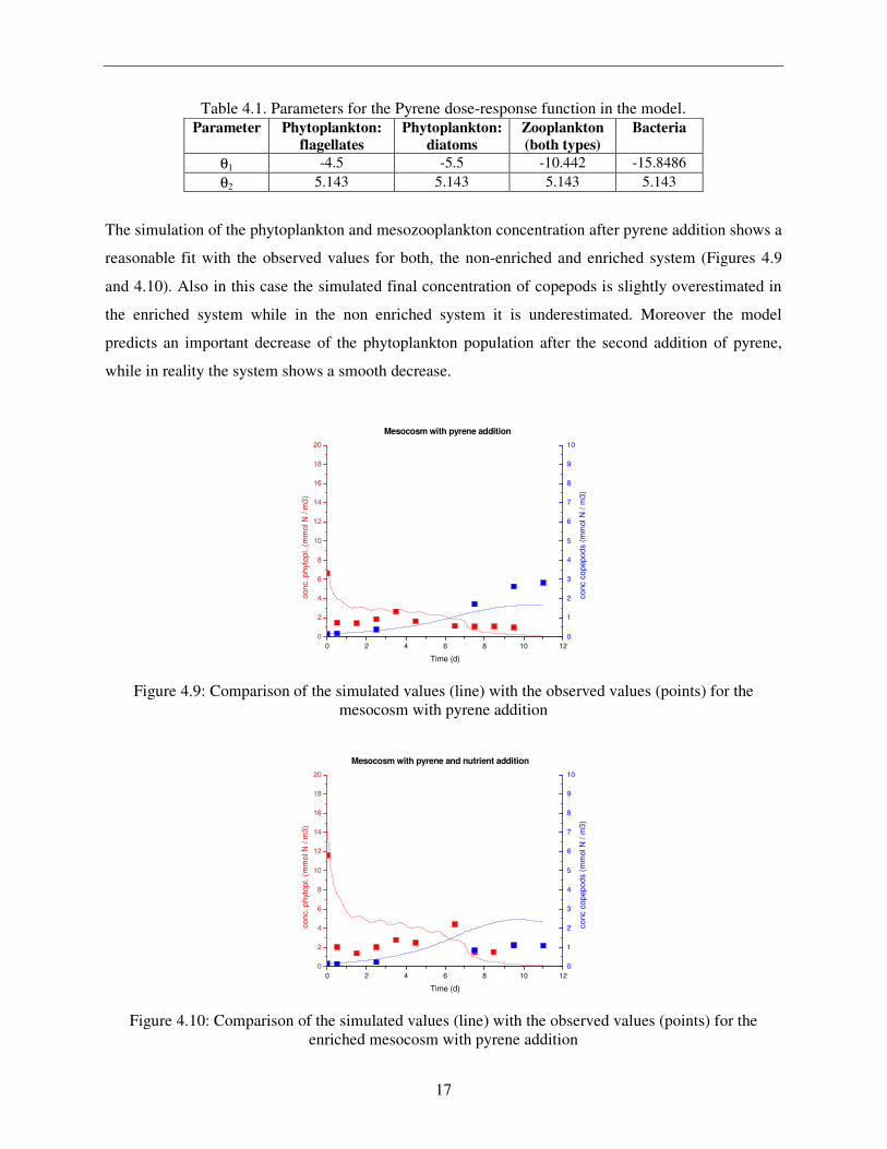
The simulation of the phytoplankton and mesozooplankton concentration after pyrene addition shows a

reasonable fit with the observed values for both, the non-enriched and enriched system (Figures 4.9

and 4.10). Also in this case the simulated final concentration of copepods is slightly overestimated in

the enriched system while in the non enriched system it is underestimated. Moreover the model

predicts an important decrease of the phytoplankton population after the second addition of pyrene,

while in reality the system shows a smooth decrease.

0 2 4 6 8 10 12

0

2

4

6

8

10

12

14

16

18

20

0

1

2

3

4

5

6

7

8

9

10

co

nc. p

hyto

pl. (

mm

ol N

/ m

3)

Time (d)

co

nc c

op

ep

od

s (

mm

ol N

/ m

3)

Mesocosm with pyrene addition

Figure 4.9: Comparison of the simulated values (line) with the observed values (points) for the

mesocosm with pyrene addition

0 2 4 6 8 10 12

0

2

4

6

8

10

12

14

16

18

20

0

1

2

3

4

5

6

7

8

9

10

co

nc. p

hyto

pl. (

mm

ol N

/ m

3)

Time (d)

co

nc c

op

ep

od

s (

mm

ol N

/ m

3)

Mesocosm with pyrene and nutrient addition

Figure 4.10: Comparison of the simulated values (line) with the observed values (points) for the

enriched mesocosm with pyrene addition

18

The effect of pyrene addition depends on the sensitivities of the different species to the pollutant and

the strength of indirect effects (Fig. 4.11). Flagellates are more affected than diatoms; therefore the

relative abundance of diatoms increases during the simulation. Indirect effects are observed on the

zooplankton growth, due to lower prey availability. The fast increase of detritus during day 1 and 2 is

caused by the death of phytoplankton after addition of pyrene, in parallel there is a smooth increase of

the bacteria population, which feeds on detritus. It is interesting to note that both addition of

contaminant are followed by a peak in detritus production.

0 1 2 3 4 5 6 7 8 9 10 11

0

2

4

6

8

10 Pf

Pd

Zs

Zl

mm

ol N

/m3

Time (days)

0 1 2 3 4 5 6 7 8 9 10 11

0

50

100

150

200

250

300

350

400

Ba

De

mg C

/m3

Mesocosm with pyrene addition

Figure 4.11: Simulation of the biomass and detritus distribution in the mesocosm with pyrene addition

Similar trends can be observed in the simulation of the enriched mesocosm (Fig. 4.12). According to

the results of the mesocosm experiment, the effect of pyrene is stronger in the enriched mesocosm.

Even though the concentration of phytoplankton is the double in the enriched system, after addition of

pyrene it decreases to the same level as the non-enriched community. These observations were

confirmed by the simulation results.

19

0 1 2 3 4 5 6 7 8 9 10 11

0

2

4

6

8

10 Pf

Pd

Zs

Zl

mm

ol N

/m3

Time (days)

0 1 2 3 4 5 6 7 8 9 10 11

0

100

200

300

400

500

600

700

Ba

De

mg

C/m

3

Enriched mesocosm with pyrene addition

Figure 4.12: Simulation of the biomass and detritus distribution for the enriched mesocosm with

pyrene addition.

5. DISCUSSION

The simulation succeeded well in representing the main direct and indirect effect observed in the

mesocosm, like the stronger effect on the enriched community and there is a change in the

phytoplankton composition due to higher toxicity for flagellates.

The simulation also highlighted that the results of the mesocosm depend on the natural conditions.

Temperature and radiation influence the primary production, while the growth of zooplankton depends

on the temperature and food availability, therefore choosing a different season for the experiment is

likely to have a strong effect on the results. The system seems to be essentially top-down regulated and

the decrease of phytoplankton in the control experiment is more likely to be caused by grazing than by

reduced nutrient availability, since the system seems not to be limited by nitrogen concentration. On

the other hand, the influence of enrichment was difficult to represent in the model, since the

concentration of nutrient during the experiment was similar for the enriched and non-enriched

mesocosm (Fig.4). Therefore in the simulations the main difference between the enriched and non

enriched system were the initial phytoplankton concentration.

6. CONCLUSIONS

The outcome of the simulation highlighted some strengths and weaknesses of the methodology. On the

one hand it showed that it is possible to represent the main dynamics observed in a mesocosm

20

experiment over a relatively short time (11 days) with a rather simplified food-web model. This

confirms that the model contains the features necessary to represent the system correctly even on a

small scale. On the other hand some of the parameters, e.g. the shape of the dose-response curve for

phytoplankton and zooplankton, had to be fitted with a very limited amount of experimental data.

More research is suitable in this field.

The difference between the enriched and non enriched communities was not that obvious to represent

in the model, because the model considers only nitrogen and the data on −− + 23 NONO and +4NH

concentrations in the enriched and non-enriched systems are similar. Since the experiments should

represent environmentally reasonable enriched conditions, excessive nutrient additions had to be

avoided. Further development of the model is required in order to represent the effect of nutrient

addition under these conditions.

21

7. REFERENCES

Barata, C., Calbet, A., Saiz, E., Ortiz, L. and Bayona, J.M. 2005. Predicting single and mixture toxicity

of petrogenic polycyclic aromatic hydrocarmobs to the Copepod Oithona davisae. Environ. Toxic.

Chem. 24(11) : 2992-2999.

Bellas, J. and Thor, P. 2007. Effects of selected PAHs on reproduction and survival of the calanoid

copepod Acartia tonsa. Ecotoxicology, 16(6):465-474.

Carafa, R., Marinov, D., Dueri, S., Wollgast, J., Ligthart, J., Canuti, E., Viaroli, P. and Zaldívar, J. M.,

2006. A 3D hydrodynamic fate and transport model for herbicides in Sacca di Goro coastal lagoon

(Northern Adriatic). Mar. Poll. Bull. 52, 1231-1248.

Dalla Valle, M., Marcomini, A., Sfriso, A., Sweetman, A.J., Jones, K.C. 2003. Estimation of PCDD/F

distribution and fluxes in the Venice Lagoon, Italy: combining measurement and modelling

approaches.Chemosphere 51, 603–616.

Dueri, S., Zaldívar, J.M. and Olivilla, A., 2005. Dynamic modelling of the fate of DDT in lake

Maggiore: Preliminary results. EUR report n° 21663. JRC, EC. pp. 33.

Erlandsson C.P., Stigebrandt A. and Arneborg, L. 2006. The sensitivity of minimum oxygen

concentrations in fjord to changes in biotic and abiotic external forcing. Limnol. Oceanogr. 51(1):

631-638.

Fleeger, J.W., Carman, K.R. and Nisbet, R.M. 2003. Indirect effects of contaminants in aquatic

ecosystems. Sci. Tot. Environ. 317: 207-233.

Hjorth, M., Dahllöf, I. Forbes, V.E. 2007. Plankton stress responses from PAH exposure and nutrient

enrichment. Sumbitted to Mar. Ecol. Prog. Ser.

Hjorth, M. 2005. Response of marine plankton to pollutant stress. Integrated community studies of

structure and function. PhD Thesis. National Environmental Research Institute, Department of

Marine Ecology/ Roskilde University, GESS, Denmark.32pp.

Ilyna, T., Pohlmann, T., Lammel, G., Sündermann, J., 2006. A fate of transport ocean model for

persistent organic pollutants and its application to the North Sea. J. of Mar. Systems 63,1–19.

Jassby, A. D. and Platt, T. 1976. Mathematical formulation of the relationship between photosynthesis

and light for phytoplankton. Limnol. Oceanogr. 21, 540-547.

Jurado, E., Zaldivar, J.M., Marinov, D. and Dachs, J. 2007. Fate of persistent organic pollutants in the

water column: Does turbulent mixing matter? Ma. Poll. Bull. 54, 441-451.

Koelmans, A.A., Van de Heijde, A., Knijff, L.M. and Aalderink, R.H. 2001. Integrated modeling of

eutrophication and organic contaminant fate and effects in aquatic ecosystems. A review. Wat.Res.

35 : 3517-3536.

22

Lancelot, C., J. Staneva, D. Van Eeckhout, J.M. Beckers & E. Stanev, 2002. Modelling the Danube-

influenced north-western continental shelf of the Black Sea. II. Ecosystem response to changes in

nutrient delivery by the Danube river after its damming in 1972. Estuarine and Coastal Shelf

Science 54, 473-499.

Marinov, D., Dueri, S., Puillat, I., Zaldivar, J.M., Jurado, E. and Dachs, J. 2007- Description of

contaminant fate model structure, functions, input data, forcing functions and physicochemical

properties data for selected contaminants (PCBs, PAHs, PBDEs, PCDD/Fs) - EUR Report n 22627

EN.

Meijer, S.N., Dachs, J., Ferna´ndez, P., Camarero, L., Catalan, J., Del Vento, S., Van Drooge, B.L.,

Jurado, E., Grimalt, J.O., 2006. Modelling the dynamic air–water–sediment coupled fluxes and

occurrence of polychlorinated biphenyls in a high altitude lake. Environ. Poll. 140, 546–560.

Oguz , T., Ducklow, H. W., Malanotte-Rizzoli, P., Murray, J. W., Shushkina, E. A., Vedernikov, V. I.

and Unluata, U. 1999. A physical-biochemical model of plankton productivity and nitrogen cycling

in the Black Sea. Deep-Sea Res. I 46, 597-636.

Scheringer, M., Wegmann, F., Fenner, K., Hungerbühler, K., 2000.Investigation of the cold

condensation of persistent organic pollutants with a global multimedia fate model. Environ. Sci.

Technol. 34, 1842–1850

Schwarzenbach, R. P., Gschwend, P. M., Imboden, D. M., 2003, Environmental Organic Chemistry,

2nd Edition, Wiley Interscience, New York.

Steele, J. H. and Henderson, E. W. 1992. The role of predation in plankton models. J. of Plankton Res.

14, 157-172.

Straile , D. 1997. Gross growth efficiencies of protozoan and metazoan zooplankton and their

dependence on food concentration, predator-prey weight ratio, and taxonomic group. Limnol.

Oceanogr. 42(6), 1375-1385.

Tang K. W., Grossart, H.-P., Yam, E.M., Jackson, G.A., Ducklow, H.W. and Kiørboe T. 2006.

Mesocosm study of particle dynamics and control of particle-associated bacteria by flagellate

grazing. Mar. Ecol. Prog. Ser. 325:15-27.

Tsapakis, M. and Stephanou, E. G., 2005. Polycyclic Aromatic Hydrocarbons in the Atmosphere of the

Eastern Mediterranean. Environ. Sci. Technol.; 39, 6584-6590.

Tsapakis, M., Apostolaki, M., Eisenreich, S., Stephanou, E. G., 2006. Atmospheric Deposition and

Marine Sedimentation Fluxes of Polycyclic Aromatic Hydrocarbons in the Eastern Mediterranean

Basin. Environ. Sci. Technol., 40, 4922-4927.

Van Nieuwerburgh, L., Wanstrand, I., Liu, J., Snoeijs, P., 2005. Astaxanthin production in marine

pelagic copepods grazing on two different phytoplankton diets. J. Sea Res. 53:147-160.

23

Wania, F., Mackay, D., 1996. Tracking the distribution of persistent organic pollutants. Environ. Sci.

Technol. 30, 390A–396A.

White, J.R., and Roman, M.R., 1992. Seasonal study of grazing by metazoan zooplankton in the

mesohaline Chesapeake Bay. Mar. Ecol. Prog. Ser. 86:251-261.

Wroblewski, J.A. 1977. A model of phytoplankton bloom formation during variable Oregon

upwelling. J. Mar. Res. 35, 357-394.

24

European Commission EUR 22952 EN – Joint Research Centre Title: Modelling mesocosm experiments Author(s): Sibylle Dueri, Dimitar Marinov, José-Manuel Zaldívar, Morten Hjorth and Ingela Dahllöf Luxembourg: Office for Official Publications of the European Communities 2007 – 25 pp. – 21 x 29,7 cm EUR – Scientific and Technical Research series – ISSN 1018-5593

ISBN 978-92-79-07402-8

Abstract

In this report, an integrated model including fate of and effects of contaminants on an ecological model

is presented. The aim is to simulate the dynamic behaviour of the mesocosm experiments carried out at

NERI (see D431-D433) to elucidate the combined effects of nutrients and contaminants at ecosystem

level. The outcome of the simulation highlighted some strengths and weaknesses of the methodology.

On the one hand it is shown that it is possible to represent the main dynamics observed in a mesocosm

experiment over a relatively short time (11 days) with a rather simplified food-web model. This

confirms that the model contains the features necessary to represent the system correctly even on a

small scale. On the other hand some of the parameters, e.g. the shape of the dose-response curve for

phytoplankton and zooplankton, had to be fitted with a very limited amount of experimental data.

More research would be necessary to elucidate this part of the model. The difference between the

enriched and non enriched communities was not that obvious to represent in the model, since the data

on −− + 23 NONO and +4NH concentrations in the enriched and non-enriched systems are similar.

25

The mission of the JRC is to provide customer-driven scientific and technical support for the conception, development, implementation and monitoring of EU policies. As a service of the European Commission, the JRC functions as a reference centre of science and technology for the Union. Close to the policy-making process, it serves the common interest of the Member States, while being independent of special interests, whether private or national.

LB

-NA

-229

52-E

N-C