Mo

dellin

g Life C

ycle Co

st for In

do

or C

limate System

s

Report TVBH-1014 Lund 2005Building Physics LTH

Dennis Johansson

Den

nis Jo

han

sson

Modelling Life Cycle Costfor Indoor Climate Systems

PrefaceI would like to thank my main supervisor Professor Lars Jensen at Building Services, Lund University for all supervision, support and help. The research project behind this thesis was initiated by Professor Anders Svensson from Building Physics, Lund University 2000, who introduced me to his research field and working area. I thank him for his initiatives, support and sharing of knowledge even though he retired in the middle of this work.

I am grateful to the financers of the project, Swegon AB (former Stifab Farex AB and PM LUFT AB), the Swedish Research Council for Environment, Agricultural Sciences and Spatial Planning (Formas, former BFR) and the Foundation for Strategic Research (SSF) through the research programme Competitive Building. I give special thanks to Swegon, where I am employed and have worked for 20% of my time. The work there, my colleagues and their sharing of knowledge and industrial experience have been very useful.

The people at Building Physics and Building Services have been close colleagues through the project and their support and expertise has been very useful. I would like to thank Professor Arne Elmroth for our discussions about methods and structure and Professor Jesper Arfvidsson for his advice and encouragement. Doctor Fredrik Engdahl was the head of my department at Stifab Farex AB in the beginning and at that point a close colleague in the research project. I would also like to thank him for the discussions and co-operation.

My research project has belonged to the national research programme Competitive Building, which is now in its second phase. One aim with Competitive Building has been to add a process aspect to building research. Competitive Building also offers a research school providing PhD courses. An aim has been to extend the amount of courses to provide the industry with people with broad knowledge about technology and process issues. Therefore, half of my research education consists of courses, which means 80 credit points of courses. The rest, 80 credit points, is associated with this doctoral thesis. I want to give thanks to the people within Competitive Building. The PhD students in this group have shared their knowledge of the building sector during study trips, courses and meetings. Professor Brian Atkin, the Programme Director of Competitive Building, has given a lot of good advice about the building sector from an international perspective and research overall. Professor Jan Borgbrant, Vice-Programme Director, has offered advice on new ways of thinking and approaching problems. Lecturer Dan

3

Gaffner, Programme Secretary, has raised many technological issues regarding the building process. The experience gained and knowledge from all the courses in the Graduate Research School and the people I have met there have also been important for me.

I am grateful for the discussions with my reference group in the beginning of the project, Professor Torbjörn Jilar, Lars Björklund and Christer Backström. A special thank goes to Doctor Tor Arvid Vik, guest researcher at our department, who shared the same research area as myself. I would also like to thank Lilian Johansson for her esthetical aspects and hours of work to get the thesis printed. Thanks also to Stephen Burke who tried hard to improve my English. I would like to offer my gratitude and thanks to Doctor and surgeon Bengt Sturesson, our chief scout, for the discussions about research methodology. Finally, I would like to thank my family, relatives and friends for their support.

4

AbstractThe indoor climate system, which serves a building with a proper indoor air quality and thermal comfort, has been predominantly designed based on the initial cost. A life cycle approach could improve both the economic and environmental performance since the energy use could decrease. There has been a lack of knowledge, models and tools for determining the life cycle cost (LCC) for an indoor climate system. The objective of this research project is to propose a model and a PC program for calculating the LCC for indoor climate systems. Focus is on indoor climate systems in Sweden for premises and dwellings. This thesis presents the LCC model and addresses some questions about input data and indoor climate system design through seven appended papers. The indoor climate systems included in the LCC model have different principles for supplying air, extracting air, recovering heat, controlling the airflow rate and supplying heating and cooling to the building. The LCC includes initial costs for purchasing and mounting the components. The LCC also includes running costs for energy, maintenance and repair. Space loss due to indoor climate system components is taken into account in the form of an annual rent loss. A work productivity cost related to ventilation airflow rate and indoor temperature can be added. A scrap value can also be added. According to LCC techniques, all future costs are discounted to the value of today, which is the net present value method. Some results from the PC program implementation in its present state are given. The results from the LCC model can help to choose the system with the lowest LCC for a particular situation. The results can also help to focus the development of indoor climate systems on parameters that are the most important to get systems with lower energy use, which can help to reach the environmental aims of society. In the future, verifications and refinements of the proposed LCC model hopefully will take place.

Keywords

indoor climate system, ventilation, HVAC, life cycle cost, LCC, energy, maintenance

5

6

SammanfattningFör att förse en byggnad med rätt luftkvalitet och temperatur behövs ett inneklimatsystem som i denna avhandling är ett samlingsnamn för ventilations-, värme- och kylsystem. Hittills har val av inneklimatsystem i byggnader mest baserats på en lägsta initialkostnad. Med ett livscykel-perspektiv borde de totala kostnaderna och miljöpåverkan från systemen kunna minskas. Modeller och verktyg för att göra livscykelkostnadsanalyser på inneklimatsystem har saknats. Detta forskningsprojekt har syftat till att föreslå en modell och ett PC-program för att beräkna livscykelkostnaden (LCC) för inneklimatsystem. Denna LCC kan användas för att välja inneklimatsystem men också vara till hjälp vid utvecklingsarbetet av inneklimatsystem för att fokusera på rätt parametrar för att nå lägre energianvändning och ett hållbarare samhälle. Avhandlingen beskriver LCC-modellen och diskuterar aspekter på ingångsdata och systemutformning genom de bifogade artiklarna, samt ger några resultat från PC-programmet i sin nuvarande form. De inneklimatsystem som behandlas är system, som förekommer i svenska kontor, skolor och bostäder. De olika inneklimatsystemen har olika principer för att tillföra luft, bortföra luft, styra ventilationsflödet, återvinna värme och tillföra värme och kyla till byggnaden. Frånluftsystem ingår med och utan frånluftsvärmepump och från- och tilluftssystem ingår med värmeväxlare. Luften kan tillföras genom uteluftsventiler, takdon, lågfartsdon, aktiva takbafflar eller fönster-apparater. För kontor kan luften bortföras i varje rum eller i varje korridor. För bostäder bortförs luften i kök och badrum. Flödet kan sättas konstant eller variabelt beroende av tiden, närvaron eller kylbehovet. I fallet med variabelt flöde kan huvudkanaltrycket hållas konstant eller sänkas om möjlighet finns. Kanalsystemet kan dimensioneras med konstant diameter för varje gren eller med konstant tryckfall per meter kanal för varje kanalbit. Värme kan tillföras byggnaden genom vattenburna radiatorer, elradiatorer, aktiva takbafflar eller fönsterapparater. Frånsett genom ventilationssystem med variabelt temperatur-styrt flöde, kan kyla tillföras byggnaden genom passiva takbafflar, aktiva takbafflar eller fönsterapparater. LCC:n inkluderar initial kostnad för att köpa och montera inneklimatsystemets komponenter. LCC:n inkluderar också framtida kostnader under hela livscykeln för energi, underhåll, reparation och förlust av hyresintäkt till följd av areaförlust. Lönekostnader eller hälso-kostnader som beror på inverkan från ventilationsflödet eller innetemperaturen kan anges liksom ett skrotvärde. Alla framtida kostnader diskonteras med nuvärdesmetoden. Avhandlingen pekar på framtida testning, förfining och utveckling av PC-programmet för att göra det lättanvänt men också på framtida forskning för att bättre förstå livscykelkostnadsproblematiken för inneklimatsystem.

7

Contents

Preface 3

Abstract 5

Sammanfattning 7

Contents 8

Nomenclature and list of symbols 11

1. Introduction 21 1.1 Objectives 23 1.2 Limitations 24 1.3 Thesis structure 25

2. Background 27 2.1 Methodology 31 2.2 Research project and Competitive Building 32

3. Appended papers 35 3.1 Paper I – A life cycle cost approach to optimising 35

indoor climate systems 3.2 Paper II – Optimal supply air temperature with respect 37

to energy use in a variable air volume system 3.3 Paper III – Optimal supply air temperature with respect 38

to energy use in a constant air volume system 3.4 Paper IV – Occupancy levels in three Swedish offices – 39

influence on energy use 3.5 Paper V – Life cycle cost regarding duct systems 41 3.6 Paper VI – Comparison between synthetic outdoor 42

climate data and readings – applicability of Meteonorm in Sweden for building simulations

3.7 Paper VII – Under-balancing mechanical supply 43 and exhaust ventilation systems with heat recovery –effects on energy use

4. LCC technique 45

8

5. LCC model for indoor climate systems and PC program 53

5.1 Level of details 55 5.2 Buildings and indoor climate systems 55 5.3 Initial costs 74 5.4 Energy costs and power need 84 5.5 Maintenance, repair and other costs 95 5.6 Aspects on algorithms and PC program 102

6. Model results 107 6.1 One corridor office building 107 6.2 School 117 6.3 Apartment building 120 6.4 Detached house 124

7. Discussion and conclusions 129 7.1 Applicability of the LCC model and PC program 129 7.2 Model results 130 7.3 Simplifications 133 7.4 LCC model and PC program refinements 134 7.5 Future research 135

8. References 137

9

Paper I 151 Johansson, D., Svensson, A. (2003), A life cycle cost approach to optimising indoor climate systems, in Construction Process Improvement, eds. Atkin, B., Borgbrant, J., Josephson, P.E., Blackwell Science, Oxford, Great Britain

Paper II 165 Engdahl, F., Johansson, D. (2004), Optimal supply air temperature with respect to energy use in a variable air volume system, Energy and Buildings, 36, pp205-218

Paper III 181 Johansson, D. (2003), Optimal supply air temperature with respect to energy use in a constant air volume system, Proceedings of the 2nd international conference on building physics, Leuven, Belgium, pp699-708

Paper IV 193 Johansson, D., Occupancy levels in three Swedish offices – influence on energy use, Submitted to Building and Environment 2005

Paper V 211 Johansson, D., Life cycle cost regarding duct systems, Submitted to Energy and Buildings 2005

Paper VI 227 Johansson, D., Comparison between synthetic outdoor climate data and readings – applicability of Meteonorm in Sweden for building simulations, Submitted toTheoretical and Applied Climatology 2005

Paper VII 243 Johansson, D., Under-balancing mechanical supply and exhaust ventilation systems with heat recovery –effects on energy use, Submitted to the Third International Building Physics Conference 2006, Montreal, Canada

10

Nomenclature and list of symbols Graphs and tables are usually formatted according to the standard, SS 01 62 16, in this thesis regarding the notation of units on graph axes and table headers. This standard means that the quantity is divided by the unit in the table header or on the axes.

Below, a nomenclature list is given with some of the words that are defined and used. After that, a list of symbols used is given.

Adjusting damper Damper used to get the intended airflow rate from all diffusers. The word balancing damper is also used

Air handling unit Subsystem bought in one unit consisting of fans, heat recovery unit, filters, control and casing to which the main silencer and main ducts are connected. It can also be called an HVAC unit.

Air inlet Air terminal usually located above or below the windows to supply air in exhaust ventilation systems

Air speed The magnitude of the air velocity vector. Air velocity is a vector quantity containing number, unit and direction.

Air terminal Generic term for supply devices and exhaust devices

Active beam Unit located in the ceiling chilled by hydronic cooling. It can be heated with hydronic heating. The word ‘active’ tells that it is also used as supply diffuser.

Branch duct The duct between the main duct and the connection duct in the duct system. It makes up the second tree level if the duct system is symbolized with a tree structure

11

CAV Ventilation system with constant airflow rate, usually interpreted as Constant Air Volume. The word volume seems to be confusing. Therefore airflow rate is used instead.

Ceiling diffuser High speed supply diffuser mounted in the ceiling without any hydronic heating or cooling features

Connection duct The duct between the branch duct and the air terminals. It makes up the third tree level if the duct system is symbolized with a tree structure.

DCV Demand Controlled Ventilation. It can be controlled by occupancy sensors, carbon dioxide sensors or other sensors. It is referred to as VAV controlled by occupancy in this thesis.

Detached house Smaller dwelling usually used by one family. It can be called a single family house.

Dwelling Building used for housing of people

Energy cost Cost for energy use

Energy price Cost for 1 kWh of energy

Exhaust device Air terminal that is made for extracting air in the exhaust part of a ventilation system

Exhaust ventilation Ventilation system with mechanical exhaust but supply air through air inlets

Hydronic system Term used when energy is distributed by hot or cold water in a pipe system

Incidence Number of added cases during a certain time period, for example number of people fallen ill during a year out of 1000 inhabitants

Indoor climate system Combination of ventilation, heating and cooling systems. It can be called HVAC system.

12

Induction unit Unit often located below the windows where the room air is induced and chilled by hydronic cooling and heated by hydronic heating. The word perimeter wall unit can be used. It is also used as supply diffuser.

Initial cost Cost occurring in the start of the life cycle

LCA Life Cycle Assessment. Investigation of the environmental load of a product over the life cycle.

LCC Life Cycle Cost

LCP Life Cycle Profit

Low speed diffuser Supply device that supplies the air at low speed to avoid mixing the air in the room. The word low velocity diffuser is also used, although there is no information about the air direction. The word displacement diffuser is also used.

Main duct The duct between the air handling unit and the branch duct. It makes up the first tree level if the duct system is symbolized with a tree structure.

Main pressure feedback Control system that takes into account the branch duct damper positions to enable a decreased main duct pressure if all branch duct dampers are more or less closed.

Maintenance cost Annual cost for maintaining the indoor climate system

Odds ratio Association measure commonly used in case-control studies. It is the ratio between the odds for a case to be in a certain condition and the odds for a control to be in a certain condition. Odds is the probability of being in a certain condition divided by the probability of not being in that condition.

13

Outer fan efficiency Fan efficiency defined based on the active electrical input power to the unit and the outer pressure drop

Outer pressure drop Pressure drop outside the fan or the air handling unit. The dynamic pressure is always lost in room ventilation.

Passive beam Unit located in the ceiling chilled by hydronic cooling. The word ‘passive’ tells that a supply diffuser is also needed.

Premises Building for commercial use like offices and schools

Prevalence Presence of cases at a certain time, for example number of sick people per 1000 inhabitants

Radiator Unit used for heating the room. It can use hydronic heating or electricity.

Repair cost Cost for replacing worn out components at certain times

Room Part of premises, apartment or detached house

Rooms with Rooms in an apartment or in a detached exhaust devices house that have exhaust devices. These are

kitchens, bathrooms, toilets and wardrobes.

Rooms with Rooms in an apartment or in a detached house supply diffusers that have supply devices. Usually these are living

rooms and bedrooms.

Running cost Cost that occurs after the start of the life cycle. These costs usually must be discounted to today’s value.

14

Specific fan power Fan power needed to get an airflow rate of 1m³/s in a ventilation system. The airflow rate refers to the maximum of supply and exhaust airflow rate. The fan power refers to the active part of the power to both fans if the supply system is mechanically driven.

Supply and exhaust Ventilation system with exhaust and supply ventilation systems both mechanically driven

Supply device Generic term for supply diffusers and air inlets

Supply diffuser Unit that supplies air in a mechanical supply ventilation system

Support heating Intentional heating that is needed to fulfil the room power balance, usually accomplished by hydronic radiators. This heating comes not from air.

Support cooling Intentional cooling, not from air, that is needed to fulfil the room power balance, usually done by active or passive beams

Timer Control system based on the date and hour of the day

Transfer unit Unit used for transferring air from an office cell to the corridor if the exhaust devices are located in the corridor on each storey

VAV Ventilation system with variable airflow rate. Is usually interpreted as Variable Air Volume. The word volume seems to be confusing. Therefore airflow rate is used instead. If the airflow rate is controlled by occupancy only, the term DCV is commonly used.

15

Quantity Description Unit

ABTA Total building floor area m²

Acap Area of thermally active mass in room m²

Aroom Room area m²

Atrans Heat transmitting area m²

Awindow Window area m²

BHF Storey height of building m

BLA Apartment length m

BLR Length of room m

BLT Building lenght m

BWC Width of corridor m

BWR Width of room m

BWT Building width m

Cadjust Cost for adjusting dampers SEK

Cbend Cost for bends SEK

Cduct Cost for ducts SEK

Ci,n Expenditure of type i that occurs year n SEK

Ci Expenditure of type i that occurs annualy SEK

Cred Cost for duct reductions SEK

Csilencer Cost for silencers SEK

CT Cost for T-junctions SEK

COPchill Coefficient of performance of a chiller -

COPHP Coefficient of performance of an exhaust heat pump -

ccap Heat capacity of the thermally active mass in room J/(kg·K)

cp Heat capacity of air J/(kg·K)

cW Heat capacity of water J/(kg·K)

Dh Degree hour °C·h

d Duct connection diameter m

dA Diameter through a T-junction m

dB Diameter branched from a T-junction m

dAHU Diameter of air handling unit connection m

dh Hydraulic diameter m

dp Pressure drop Pa

dpduct Pressure drop for ducts Pa

16

dpbend Pressure drop for bends Pa

dphr Pressure drop for heat recovery unit Pa

dpouter Pressure drop per side outside the air handling unit Pa

dpouter_ex Exhaust pressure drop outside the air handling unit Pa

dpouter_sa Supply pressure drop outside the air handling unit Pa

dpTe2Branched pressure drop in T-junctions in exhaust systems

Pa

dpTe3 Pressure drop through T-junctions in exhaust systems Pa

dpTs2 Branched pressure drop in T-junctions in supply systems Pa

dpTs3 Pressure drop through T-junctions in supply systems Pa

dtfan_sa Supply air temperature raise from supply fan °C

I Number of different costs -

i Type of cost index -

k Discount interest rate change constant 1/year

kleak Leakage airflow rate at 50 Pa pressure difference l/(s·m²)

ksolar Radiation transmittance -

L System curve for fans -

LB Length between connection ducts m

LC Length of connection duct m

Lduct Length of duct m

LM Length between branches m

LPC Length of connection pipes m

Lpipe Length of pipes m

LPD Length of distribution pipes m

LPS Length of stack pipes m

LCC Life cycle cost SEK

mcap Thermally active mass for the interior in room kg

N Life span year

n Annual time year

nrexhaustNumber of rooms with exhaust devices in an apartment or detached house

-

nrsupplyNumber of rooms with supply diffusers in an apartment or detached house

-

nrfexhaustNumber of rooms with exhaust devices on a storey in a detached house

-

nrfsupplyNumber of rooms with supply devices on a storey in a detached house

-

17

nstorey Number of storeys -

NPVi Net present value of expenditure Ci SEK

NPVi,n Net present value of expenditure Ci,n SEK

NPVn Net present value of sum of expenditures Ci,n SEK

OC Occupancy rate -

Pair Power for heating ventilation air W

Paircool Power for cooling ventilation air W

Pbeam Power of direct radiation towards sun W

Pcap Power from heat capacitor to room W

Pcooling Power for cooling W

Pdiffuse Power of diffuse radiation horizontally W

Pfan Electrical fan power W

Pfan_ex Electrical exhaust fan power W

Pfan_sa Electrical supply fan power W

Pheating Power for heating W

PHP_gain Gained power from heat pump W

PHP_in Electrical input power to heat pump W

Pint Internal power gain W

Pleak Outgoing power caused by leakage W

Ppump Electrical pump power W

Psaved Saved heating power by heat recovery W

Psolar Power from solar radiation to room W

Psupport Power from support cooling or heating W

Ptrans Power transmitted from room W

Pvent Power from supply air to room W

Pwatercool Water cooling power W

PDtRelative decrease in productivity from indoor temperature

-

PIslRelative increase in productivity due to decreased short term sick leave from airflow rate

-

PIwpRelative increase in productivity due to work productivity from airflow rate

-

PIqRelative increase in productivity due to decreased short term sick leave and increased work productivity

-

pd Dynamic air pressure Pa

ps Static air pressure Pa

18

q Airflow rate m³/s

qex Exhaust airflow rate m³/s

qleak Actual average leakage airflow rate m³/s

qref Reference airflow rate for productivity estimation m³/s

qsa Supply airflow rate m³/s

qvent Ventilation airflow rate m³/s

R Pressure drop per meter duct Pa/m

rci,n Nominal price change rate for cost i at year n -

rdi Discount interest rate -

rdi,n Discount interest rate at year n -

rn,n Nominal rate of interest at year n -

rpi,n Real price change rate for cost i at year n -

rr,n Real rate of interest at year n -

t Temperature °C

tcap Temperature of thermally active mass in room °C

tex Exhaust air temperature °C

thr_in Temperature after heat recovery unit on supply side °C

thr_out Temperature after heat recovery unit on exhaust side °C

tref Reference temperature for productivity estimation °C

troom Room temperature °C

tsa Supply air temperature °C

tout Outdoor temperature °C

tout,i Outdoor temperature at annual hour i °C

Uav Average transmittance for the building envelope W/(m²·K)

v Air speed m/s

v1 Air speed at T-junction m/s

v2 Air speed at T-junction m/s

v3 Air speed at T-junction m/s

Wfan Annual fan energy use Wh

Wheat Total heating energy Wh

Wsaved Annually saved energy from heat recovery Wh

Angle between window normal and sun beam direction -

fan Outer fan efficiency -

fan_ex Outer exhaust fan efficiency -

fan_sa Outer supply fan efficiency -

19

heat Efficiency of heating plant -

hr Temperature efficiency of heat recovery -

pump Water pump efficiency -

Density of air kg/m³

Time s

20

1. Introduction People spend up to 90% of their time indoors (Sundell and Kjellman, 1994; Lech et al. 1996). Most of our time indoors is divided between work and home with the remainder being in premises, shops and even a small amount inside vehicles. To ensure people’s health and comfort when they are indoors, the indoor air quality and thermal comfort must be appropriate. An indoor climate system serves this purpose (Svensson, 2003; Nilsson, 2003b; Goodfellow and Tähti, 2001; Boverket, 2002).

In the context of this thesis, the indoor climate system consists of ventilation, heating and cooling systems to provide a building with a good thermal comfort and indoor air quality. In a particular situation, several different indoor climate systems can most often be used. Figure 1.1 shows a normal indoor climate system for an office building in Sweden. Due to demands such as the EU Directive on the Energy Performance of Buildings (European Commission, 2005) or the Kyoto protocol (UNFCCC, 2005), the ability to only handle the functional requirements is not enough. The indoor climate system must also use as little resources as possible, where energy is one type of resource. As a general rule, the built environment sector in Sweden currently uses about 40% of the total energy used in the country (Statens Energimyndighet, 2005). A part of this energy is used to provide buildings with the energy required for heating, ventilation and cooling.

Economical resources are in focus and can be handled by the use of life cycle costing. The Life Cycle Cost (LCC) is the sum of all costs during the entire life cycle of the indoor climate system. The LCC can be a basis for comparisons between different indoor climate systems and system designs. There are a number of programs and some helpful literature for calculating LCC. However, there is a lack of models and tools specifically produced for calculating the LCC for indoor climate systems during the early stage of the building design process. This is when the indoor climate system should be designed.

21

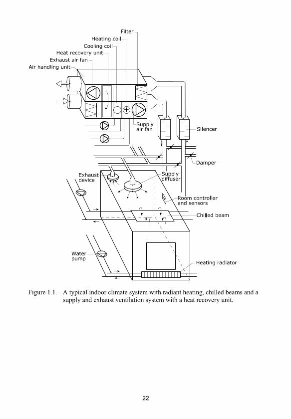
Figure 1.1. A typical indoor climate system with radiant heating, chilled beams and a supply and exhaust ventilation system with a heat recovery unit.

22

Figure 1.2. Here, system A is compared with system B, but in reality there will be more than two indoor climate systems in the comparison. The LCC model helps to choose the system based on the lowest LCC.

1.1 Objectives

The overall objective of this research project is to propose a model to do LCC calculations on indoor climate systems early in the building design process. The LCC should basically be done in the context of the building owner. A second objective is to produce a tool based on the model. This tool is in the form of a PC program, which can be used to calculate LCC for indoor climate systems. The result will be a model and a PC-program which can be used to choose and optimize the indoor climate system from an LCC perspective.

To enable the use of the model at an early stage in the building design process, the need for input data should be reasonably low. The model handles different systems that are common in Sweden and different control strategies for these systems. The buildings that are taken into account are residential buildings, office buildings and school buildings. All indoor climate systems must fulfil general requirements to get an appropriate indoor climate. Figure 1.2 illustrates the project approach.

23

The model helps calculate the initial costs and running costs for a number of typical Swedish indoor climate systems for premises and dwellings. Initial costs include material and labour costs for purchasing and mounting the equipment. Running costs include energy costs, maintenance costs, repair costs and costs for space loss. Energy cost is based on the energy use of fan electricity, heating energy and cooling energy. The energy use is simulated for the particular, chosen building and indoor climate system. The maintenance cost and the repair cost are estimated from the initial cost. It is possible for the user of the PC-program to insert the scrap value and costs related to the work or health performance as a result of a certain indoor temperature or airflow rate. All running costs are discounted with the LCC technique.

1.2 Limitations

This LCC model will not deal with some of the problem areas of modelling the LCC for indoor climate systems

Life Cycle Assessment (LCA) is not dealt with in this research project The LCC technique is used as a tool and not evaluated further. In a broader view, the indoor climate could also include indoor lighting, sound or social factors, but it does not. The term HVAC system could have been used; however, the term indoor climate system is preferred, as it clearly takes into account more than just the HVAC unit. The LCC model does not include an analysis of the energy supply system. Therefore, the energy supply system is modelled in a simple way. There are a lot of different indoor climate systems. Only a limited number of systems are reasonable to include. Since the focus of this project has been the building industry in Sweden, indoor climate systems, buildings, prices and outdoor climates are from a Swedish context. The approach used in this thesis could be applied to other locations. The differences between manufacturers of indoor climate system components are not analyzed. Therefore, products from several manufacturers spread over the Swedish market are used for input data. Natural and hybrid ventilation systems are not considered, as they are already the subjects of theses (Jenssen, 2003; Kleiven, 2003; Vik, 2003). Furthermore, the building integration of those systems is so high that, to avoid designing complete houses, object studies could be used instead of a theoretical approach.Industrial buildings will not be considered, since they depend on the industrial process. Therefore, they are difficult to generalize. The building design and technology will influence not only the costs of the indoor climate system but also the costs of the building itself. The change

24

in building costs will not be considered in the LCC model, which means that the LCC model can not optimise the indoor climate system together with the building. For example, thicker insulation in a dwelling should lower the amount of energy used for heating thus lowering the power need for heating. This would result in smaller and less expensive indoor climate system components but would increase the cost of insulation. This LCC model takes into account the influence on the indoor climate system components and on the energy use for heating but it does not take into account the higher insulation cost.

1.3 Thesis structure

This thesis starts with an overall introduction of the objectives followed by some background and literature review in Sections 1 and 2. Section 3 gives short summaries of the appended papers and their relationship to the LCC model and its input data. Section 4 reports on the economic techniques used in the LCC model to calculate the LCC. Section 5 describes the LCC model build up and the PC program. Section 6 gives some examples of calculations performed applying the LCC model on typical buildings. Section 7 discusses the LCC model development and the LCC model’s results. Conclusions are also given and future research is addressed.

Seven research papers are appended in this thesis. The appended papers establish background theories and data for the LCC model and give examples of LCC and energy related issues regarding indoor climate systems. Papers I-III are published and Papers IV-VII are submitted to be published.

25

26

2. Background To obtain good indoor air quality and good thermal comfort, temperature levels and airflow rates need to be determined. Determining a good airflow rate is not a straightforward procedure, since we still do not know very much of its effects on human beings. For example, carbon dioxide is generated by human beings and can be used as an indicator of the indoor air quality. However, a number of other substances are emitted from the building’s materials, human beings and processes that take place indoors. There are also a number of other substances in the outdoor air. It is difficult and expensive to measure these substances and simplifications are needed to set the required supply airflow rate.

Specifications of the indoor climate regarding thermal comfort and air quality are determined by requirements, recommendations, national regulations or by the building’s user. This helps to simplify the design process of an indoor climate system. Furthermore, from a historical perspective, politics and resources have also influenced these demands. Usually, the minimum and maximum temperatures and the supply airflow rate are set depending on the activity in the building.

One problem in the design of an indoor climate system is that there has been a predominant focus on initial costs. A life cycle approach could improve both the energy and economic performance of the indoor climate system. Even though many actors are present with different economical interests in different parts of the building process and the building’s life cycle, the interest for LCC analyses seems to have increased over time. The clients and building owners seem to be more aware of the future costs. The manufacturers see an opportunity to use life cycle costing to sell more energy efficient products and solutions on the market. In the future, the interest for energy use seems to increase even more. It can be believed that the legal requirements turn towards a low energy focus in a way that the involved persons in the building process cannot avoid the broad picture as much as before.

A number of LCC models are available and some are for indoor climate systems. However, many of them handle only a part or some parts of the indoor climate system. In Sweden, a popular model for do an LCC analyses on a routine basis is called Energy Efficient Procurement, ENEU 94 (Sveriges Verkstadsindustrier, 1996), which has been updated to a web-based version called “LCC Energi” (Sveriges Verkstadsindustrier, 2001). This is a form-based guideline, in which the contractors have to calculate the LCC in a

27

procurement situation. If many contractors attend to the procurement, a ventilation system with a low LCC is likely to be found, but this is not always the case. “LCC Energi” handles a number of details in the air handling unit, such as heat recovery unit efficiency and a correction term for freezing in the heat recovery unit. Still, external programmes for calculating the initial costs of the system, the energy demand, and pressure drops are needed.

Using ideas from ENEU 94, an EU-supported project has drawn up similar guidelines. This SAVE project, known as “LCC-based Guidelines on Procurement of Energy Intensive Equipment in Industries” (Eurovent, 2001), adopts the manufacturer’s point of view instead of that of the client or building owner. One problem with both sets of guidelines is the lack of options for modelling either the entire indoor climate system or different control strategies.

Gustafsson and Karlsson (1988) pointed out the importance of using life cycle costing when retrofitting buildings. They discussed the importance of considering an entire apartment block as an energy system and that certain actions on the heating system can make other modifications to the envelope unprofitable. Gustafsson and Karlsson (1989) gave a method for combining the retrofits of the building envelope, heating system and ventilation system.

Arditi (1996) conducted a survey that showed that 40% of the municipalities in the US used LCC analyses to some extent in construction projects including more than buildings. The reasons given for not using these analyses were the absence of guidelines and the difficulty of estimating future costs. Sterner (2000) showed that 66% of clients used LCC analyses to some extent in projects in Sweden in 1999 but rarely in all phases of their building projects. A significant reason for this low rate of use was the lack of tools and knowledge.

A PC programme that performs LCC analysis was presented by Ruegg and Petersen (1985). This programme calculates the LCC and a number of other economic factors. However, since it does not focus on indoor climate systems, it requires a problem definition and a definition of the alternatives by the user. Lewald and Karlsson (1988) examined the LCC for electrically heated houses to determine if it would make sense to change to a hydronic system. James and Phillips (1992) presented a spreadsheet application for the purpose of separating the HVAC system from the building, but it does not calculate the energy demands or different HVAC systems. Tozer et al. (1999) examined the LCC for indoor climate system regarding thermodynamics and exergy. Cao and Cao (2005) analysed the optimal design of thermal storage systems for boiler plants. They developed a computer program for this purpose. Lutz et al.

28

(2005) discussed LCC analysis of residential furnaces and boilers. They showed that a reduction of LCC was possible with more efficient products.

A number of different economic techniques, regarding LCC for insulation materials depending on thickness, were discussed by Al-Hammad and Fahd (1992). One of the preferred techniques was the net present value method. The researchers did not discuss either how to calculate the energy demand or the effects of different indoor climate systems. LCC analysis methodologies were analyzed by Durairaj et al. (2002). They did not discuss buildings in particular and state that there is a need for several LCC models for different application areas. Often, constant maintenance and repair costs are assumed in LCC analyses. Karyagina et al. (1998) stated that these assumptions often lead to over-simplifications in the LCC analysis and incorrect results. They used statistical methods to specify the system failure and LCC for a number of Computer Numerically Controlled (CNC) machines.

The LCC for semiconductor circuits was discussed by Riedel et al. (1998). They differentiated simpler semiconductor circuits from more complex semiconductor circuits. For the simpler, the reliability can be high enough to cover the lifetime of the system. For the more complex, there can be need for a lot of maintenance. Guidelines were developed by Tighe (2001) for choice of pavement based on LCC. A lognormal distribution was incorporated to describe the parameters in an appropriate way. Fan system design in agricultural buildings was discussed by Christianson and Fehr (1983). Both physiological and economical considerations were discussed. Malinowski (2004) discussed the LCC of electrical motors and their drives. He pointed out the benefit with adjustable speed drives regarding energy and motor life time. Motor bearing lubrication methods and their impact on the LCC was evaluated by Hodowanec (1999). The over-sizing of pumps and the influence on the LCC was discussed by Wheatley (2002). Measures used in the UK for better pump design was given.

Ståhl and Wallace (1995) looked at an older and a newer cooling system for telecom equipment buildings from a LCC perspective. They found that the newer system gave a lower LCC, a lower energy use and better performance. Optimal insulation thickness for building envelopes was derived by Hasan (1999) taking into account heat transmission and insulation costs. Hens et al. (2002) investigated the optimal insulation thickness of a building with regards to the fact that the users of a building adjust indoor temperatures according to their energy bills. The real savings from additional insulation decreased, since people increased the indoor temperature when their energy costs decreased. Florides et al. (2002) and Anger and Nilsson (2004) analysed measures to

29

lower the energy use in buildings. It was shown that energy saving measures were profitable if they are applied to new houses.

Nilsson (1995) compared the LCC for different air handling units. He found that the LCC was not influenced much by the size of the air handling unit even if there was a minimum for a certain size. He concluded that use of LCC should not be enough to lower the energy use. He also concluded that a good ventilation system design should result in a specific fan power value of between 0.5 and 1 kW/(m³/s). Sellers (2005) discussed air handling unit design and sizing. He pointed out the importance of the fan and the filters for the energy use. He stated that the sizing of air handling units is a value-added engineering process.

Öfverholm (1998) did a broad analysis of the life cycle costing for buildings. He presented methods and problems with that approach although he never focused on indoor climate systems or building services. He found a need for more input data with a good structure regarding costs. He also refered to a model used for the procurement of transformers in the electric power industry. This model has apparently increased the energy performance of transformers and has made these transformers more profitable for the manufacturers.

Vik (2003) looked at the life cycle costs for hybrid ventilation systems. They incorporated the building in a higher extent than mechanical systems. He compared different solutions, also with a typical mechanically ventilated building, and described a method to calculate LCC. Since the building structure and envelope is a part of the ventilation, he discusses cost allocation a lot. The result showed no large difference between mechanical and hybrid ventilation systems.

An example of a computer program that handles the air handling unit is a manufacturer’s program (PM-Luft, 2005). The disadvantage is that it does not include initial costs and does not handle the rest of the indoor climate system although the air handling unit is handled in a detailed way.

A Swedish consultant has made an Excel sheet for comparing different air handling unit locations and solutions in office buildings (Swegon, 2005). It takes into account effects on the building envelope and structure but does not incorporate the rest of the indoor climate system. Particularly, there is a remarkable influence on the LCC if the air handling unit is located in the basement and excavation work is needed to fit the air handling unit into place.

30

2.1 Methodology

This LCC model for indoor climate systems is based on a theoretical approach. It uses empirical data for components that are put together to form different indoor climate systems. Typically defined components can be split into subcomponents. These components can also be grouped together to form super components. The question is on what size level the components should be specified. Components that are too large would hide differences that affect the LCC. Components that are too small would need a lot of data and would not be needed to separate the different indoor climate systems. By this approach, parameters such as outdoor climate can be handled by calculations and simulations. If the components are small enough, the use of the LCC model can result in simplifications being made in order to get a less detailed model. This would be difficult to test without first having the detailed model.

An alternative approach would be to use measured data from empirical objects, which means real buildings. That would provide realistic data, at least for the particular object where the data came from. The question is if such data are generally valid. Since different systems will be compared, there is a need for experience data from buildings including the compared indoor climate systems. For stochastic reasons, there would be a need for a number of buildings with each indoor climate system. It would be difficult to find enough valid or reliable objects with traceable costs for each part of the indoor climate systems to obtain significant results. The multitudes of parameters that influence the life cycle cost need to be matched with the collected cases, which yields a lot of cases to collect data from. This seemed to be an impracticable way. It would also be impossible to test non-existing indoor climate systems.

An LCC model incorporates both hermeneutical and positivistic aspects. The hermeneutic aspects include interpretation of human behaviour related parameters such as costs or interest rates. The positivistic aspects include the physics and the technical systems. The focus in this project has been on the positivistic parts while the human dependant data are supposed to be known from experience or supplied by the user of the LCC model.

Positivistic research usually tries to predict the future or describe the nature to make predictions possible later on. Parts of this thesis are predictable while other parts are more descriptive. This research project has been a broad project where the problem has been to put a model together with experience and knowledge from several different areas. This differs from some traditional research projects, where a narrow field is analyzed in deep detail.

31

2.2 Research project and Competitive Building

The PhD students of the Competitive Building research program, to which this project has belonged, developed a building process map during 2004. Figure 2.1 shows this process map. The aim of this map was to try to make a tool where the PhD students could locate their research projects and correlate it to others, to illustrate the research area of the research programme and to make updates to the process map and analyze how the process changes over time.

The process map is built up from a circle with two polar axes. The angle describes the product life cycle from definition and design to the end of the product use. The endless circle is meant to indicate the need for knowledge feedback from one project to another. The radius describes the ‘actors’ that take part in the process. The actors are the customer, who buys the product, the organisation, who makes the product, and society, which set the limits and requirements for the product and the process. The customer can be the building owner. The product can be an entire building or parts of a building. The organisation is the building industry.

In this project, the product can be seen as the indoor climate system. The aim is that the LCC model will be used in the early design process stage, which occurs between the product definition and the product design. The customer is the one who is going to pay. The organisation includes the ones who are going to use the LCC model or PC program. Society sets the requirements regarding the indoor climate system. This thesis focuses on the LCC model for the product with an interface to both the customer and the organisation. That means that the research project could cover the area indicated in Figure 2.1.

32

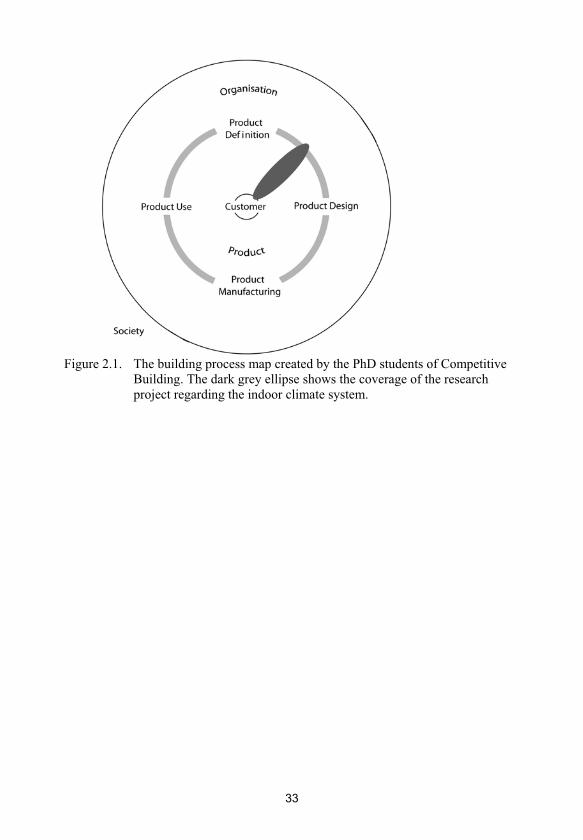
Figure 2.1. The building process map created by the PhD students of Competitive Building. The dark grey ellipse shows the coverage of the research project regarding the indoor climate system.

33

34

3. Appended papers The appended papers supplement the LCC model with input data and simplifications. Together with the rest of the thesis, the seven papers provide a view of LCC modelling for indoor climate systems and the data behind such calculations including some different system aspects that mainly influence the energy use.

The research methods for this thesis and the relationship to other research projects needed to be determined and stressed. Paper I reports on these issues, describes some literature and lays the foundation for the research project. Paper II presents a theory for an optimal supply air temperature for a VAV ventilation system, which is an example of how different control strategies can influence energy use and, in turn, the LCC. This paper is also part of another doctoral thesis (Engdahl, 2002). Both authors contributed equally. The optimisation of the supply air temperature for CAV systems has less parameters since the airflow rate is constant. This is analyzed in Paper III.

Paper IV deals with occupancy levels, which is one of the key issues when choosing a demand controlled ventilation system. The duct system design and optimisation is analyzed in Paper V. To simplify the LCC model, a simple duct design approach was needed. This approach should be appropriate for Swedish ventilation systems, still providing a solution with an LCC as low as reasonable. Outdoor climate data is needed for energy use and power need calculations. Such data can be found from simulation programs. Paper VI compares a climate data simulation program with measured Swedish data. Paper VII examines the unintentional building envelope leakage depending on the difference between exhaust airflow rate and supply airflow rate. In the LCC model, the results are used for leakage calculations.

3.1 Paper I – A life cycle cost approach to optimising indoor climate systems

This paper presents a literature review and the wishes of the building sector regarding an LCC model. It is clear that research is needed in this field to approach the LCC analysis for indoor climate systems from a system perspective. In practice, LCC analyses often mean that a comparison has been made between two alternatives. On rare occasions, a more extensive analysis is performed. The building industry also needs general knowledge about which system to choose in a given situation.

35

The paper presents the problem and the methods used in the research project. An LCC model should be able to predict the future. A number of input data are positivistic and can be predicted. However, some input data, such as interest rates or changing activity in a building, depend on human activities, which is difficult to predict. To be able to develop an LCC model for indoor climate systems, reasonably applicable system in a given building with a given activity and location must be defined and investigated. Thereafter, calculations with plausible input data must be carried out.

To determine the use of LCC calculations and to establish some relations to people from industry, 61 questionnaires were sent out to investigate the use of LCC calculations during the design of services for buildings. The response rate was 39%. Of the total number of respondents, 31% used life cycle cost analyses to some extent. Figure 3.1 shows the use of LCC analyses among consultants, private sector clients and municipalities as clients when building services are being designed. Most of the answers supported the need for better tools and also indicated that energy use is a very important issue. Life cycle costing was expected to gain more interest in the future.

0%

20%

40%

60%

80%

100%

Municipalities Private

clients

Consultants

Do not use LCC

analyses

Do use LCC

analyses, typically

in 20% of the

projects

Figure 3.1. The use of LCC analyses in the Swedish building sector during the design of building services. The bar ‘Municipalities’ means the local authorities as clients. The response rate was low; 24 of 61 returned questionnaires. However, the indication is that LCC analyses are seldom used.

36

3.2 Paper II – Optimal supply air temperature with respect to energy use in a variable air volume system

A ventilation system with variable airflow rate can be used to save energy by only supplying air when needed. Both occupancy and a need for cooling can be used to increase the airflow rate. The airflow rate, the supply air temperature and the supply air moisture content can be optimised together. The moisture content of the supply air is a topic for future analysis. However, the supply air temperature was analysed in this paper.

The power demand as a function of the supply air temperature was examined for a ventilation system with variable airflow. In one example, the internal heat load was assumed to be 500 W, the specific fan power 2 kW/(m³/s), the room temperature 25°C, the heat transfer to the outside 20 W/°C, the minimum airflow rate 10 l/s and the Coefficient Of Performance (COP) of the chiller 3. The outdoor temperature was 20°C and the relative humidity 75%. A low airflow rate needs a lower supply temperature with condensation as the result. Figure 3.2 shows the results. The temperature at the minimum power was found just before condensation occurred.

0

50

100

150

10 12 14 16 18

Supply air temperature (°C)

Power (W)

Total power

Cooling total

Cooling due to

condensation

Electrical fan

power

Figure 3.2. Power needed to cool an office cell depending on the supply air temperature for a ventilation system with variable airflow.

The paper presents a theory in order to find the optimal supply air temperature. The amount of energy saved was estimated. It was also confirmed that office cells with rather high internal heat loads during the time they are occupied still need a lot of heating at night. It should be possible to design a control algorithm, although this was not stressed.

37

No LCC influence was calculated for in the paper. For the climate in Sturup, the optimal supply air temperature compared to the best constant supply air temperature would save 1.8 kWh/m² annually if the internal heat load is 44W/m² during daytime. With an electricity price of 0.8 SEK/kWh, the saving decreases the running cost by 1.44 SEK/(m²·year) in today’s value. Over a 40 year life span with 2% discount interest rate, this would result in a net present value saving of 39.4 SEK/m². This value can be spent on a higher initial cost, still resulting in the same LCC. The exemplified scenario has low difference between the optimal energy use and the compared energy use. A different scenario where the internal heat loads vary would save more energy and allow a higher initial cost increase for a system that can set the optimal supply air temperature.

3.3 Paper III – Optimal supply air temperature with respect to energy use in a constant air volume system

A ventilation system with a constant airflow rate was combined with radiators for heating and chilled beams for cooling. This is a common indoor climate system shown in Figure 1.1. Energy is supplied to heat or cool the air depending on the outdoor temperature, the heat recovery unit and the supply air temperature. To get the room in power balance, energy is also supplied to the radiators or to the chilled beams. There is a risk that the chosen supply air temperature results in a need for cooling the air and heating the room at the same time. The opposite can also occur, which means that the air is heated and the room cooled at the same time.

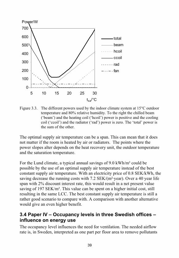
An optimally set supply air temperature would avoid both heating and cooling at the same time with different parts of the indoor climate system. The paper presents theory for an optimal supply air temperature for this system. Energy use estimations are also given for three Swedish locations. Figure 3.3 shows the power need for the different components as a function of the supply air temperature. Between 13°C and 15°C there is a constant minimum in the total power use.

38

0

100

200

300

400

500

600

700

5 10 15 20 25 30

tsa/°C

Power/W

total

beam

hcoil

ccoil

rad

fan

Figure 3.3. The different powers used by the indoor climate system at 15°C outdoor temperature and 80% relative humidity. To the right the chilled beam (‘beam’) and the heating coil (‘hcoil’) power is positive and the cooling coil (‘ccoil’) and the radiator (‘rad’) power is zero. The ‘total’ power is the sum of the other.

The optimal supply air temperature can be a span. This can mean that it does not matter if the room is heated by air or radiators. The points where the power slopes alter depends on the heat recovery unit, the outdoor temperature and the saturation temperature.

For the Lund climate, a typical annual savings of 9.0 kWh/m² could be possible by the use of an optimal supply air temperature instead of the best constant supply air temperature. With an electricity price of 0.8 SEK/kWh, the saving decrease the running costs with 7.2 SEK/(m²·year). Over a 40 year life span with 2% discount interest rate, this would result in a net present value saving of 197 SEK/m². This value can be spent on a higher initial cost, still resulting in the same LCC. The best constant supply air temperature is still a rather good scenario to compare with. A comparison with another alternative would give an even higher benefit.

3.4 Paper IV – Occupancy levels in three Swedish offices – influence on energy use

The occupancy level influences the need for ventilation. The needed airflow rate is, in Sweden, interpreted as one part per floor area to remove pollutants

39

from building and interior materials and a second part per person to remove pollutants generated by people and provide people with outdoor air. That means that the airflow rate is linear to the occupancy. When it comes to fan electricity, the needed power is not linear to the occupancy since the pressure drop is not constant. Therefore, the occupancy level distribution is needed and not only the average. The internal heat loads also depend on the occupancy levels.

This paper reports on measured occupancy rates with occupancy sensors to get data to use in the LCC model. The fan energy use is analyzed depending on different occupancy distributions. It was shown that a plausible simplification would be to use one average occupancy level during working time and another average occupancy rate during the remaining time. Figure 3.4 shows the occupancy rates for the different rooms in the monitored buildings.

Occupancy rate / %

0

10

20

30

40

50

60

70

80

MP

O1

MP

O2

MP

O3

MP

O4

MP

O5

MP

O6

MP

O7

MP

O8

MP

O A

v

UD

1

UD

2

UD

3

UD

4

UD

5

UD

6

UD

7

UD

Av

IO A

v

To

t a

v

Difference in occupancy between all-time and daytime

Occupancy all-time

Figure 3.4. The occupancy rate for the different cells in the municipality planning office (MPO), the University department (UD) and the industrial office (IO). ‘MPO Av’ is the average occupancy for MPO as ‘UD Av’ and ‘IO Av’ respectively. Daytime means between 08.00 and 18.00, Monday through Friday. All-time means the whole measured period. Since the upper part of each bar shows the difference between daytime and all-time, the lower and upper parts of each bar together means the daytime occupancy

40

3.5 Paper V – Life cycle cost regarding duct systems

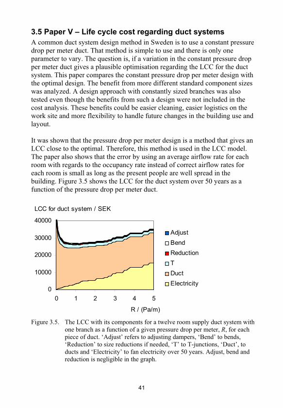
A common duct system design method in Sweden is to use a constant pressure drop per meter duct. That method is simple to use and there is only one parameter to vary. The question is, if a variation in the constant pressure drop per meter duct gives a plausible optimisation regarding the LCC for the duct system. This paper compares the constant pressure drop per meter design with the optimal design. The benefit from more different standard component sizes was analyzed. A design approach with constantly sized branches was also tested even though the benefits from such a design were not included in the cost analysis. These benefits could be easier cleaning, easier logistics on the work site and more flexibility to handle future changes in the building use and layout.

It was shown that the pressure drop per meter design is a method that gives an LCC close to the optimal. Therefore, this method is used in the LCC model. The paper also shows that the error by using an average airflow rate for each room with regards to the occupancy rate instead of correct airflow rates for each room is small as long as the present people are well spread in the building. Figure 3.5 shows the LCC for the duct system over 50 years as a function of the pressure drop per meter duct.

LCC for duct system / SEK

0

10000

20000

30000

40000

0 1 2 3 4 5

R / (Pa/m)

Adjust

Bend

Reduction

T

Duct

Electricity

Figure 3.5. The LCC with its components for a twelve room supply duct system with one branch as a function of a given pressure drop per meter, R, for each piece of duct. ‘Adjust’ refers to adjusting dampers, ‘Bend’ to bends, ‘Reduction’ to size reductions if needed, ‘T’ to T-junctions, ‘Duct’, to ducts and ‘Electricity’ to fan electricity over 50 years. Adjust, bend and reduction is negligible in the graph.

41

3.6 Paper VI – Comparison between synthetic outdoor climate data and readings – applicability of Meteonorm in Sweden for building simulations

To be able to calculate the energy use and power demand of a building, data on the outdoor climate is needed. A common resolution of outdoor climate data for building simulations is one hour between the readings. Figure 3.6 shows the temperature frequency for two locations in Sweden according to measurements made by SMHI, the Swedish Meteorological and Hydrological Institute. The temperature frequencies are stratified into different daily time intervals.

Temperature frequency/(h/°C)

0

100

200

300

400

500

600

-30 -10 10 30

Outdoor temperature/°C

Lund 24 hour

Frösön 24 hour

Lund 08-17

Frösön 08-17

Figure 3.6. The annual temperature frequencies in Lund (southern Sweden, 55°42’N, 13°11’E) and Frösön (central Sweden, 63°11’N, 14°30’E). The upper curves are for all hours and the lower curves are for daytime hours. The period measured was 1991-2001. The measurements were made by SMHI, the Swedish Meteorological and Hydrological Institute.

To be able to use the LCC model for many locations, the simulation program Meteonorm (Meteotest, 2003) was used to provide the LCC model with hourly outdoor climate data. This paper compares measured data from SMHI between 1991 and 2001 with simulated data from Meteonorm. It is not necessary that the average of the measured values is the same as the average simulated value since the next year will most likely not be an average year. It is important that the simulated data is close to the real data and that the extreme values are reasonably close. It should be better to use a simulated climate for a specific location than to use measured data from another location. The paper shows

42

that the simulated data should be possible to use. Figure 3.7 gives the error in degree hours for heating for the four compared locations. There seems to be a systematic error for the temperatures over the day that should be taken into account if outdoor climate data corrections will be made to compare measured energy use after the building is completed.

Error in degree hours for heating / ((°C·h)/h)

-1

0

1

2

1 5 9 13 17 21

Kiruna

Frösön

Lund

Stockholm

Figure 3.7. The annual error in degree hours split into each hour of the day as the simulated value minus the measured. The value at 17.00 refers to the hour before, which means 16.00 to 17.00. The summed error is divided with 365 to give the error per hour.

3.7 Paper VII – Under-balancing mechanical supply and exhaust ventilation systems with heat recovery – effects on energy use

A building located where it is usually colder than the desired indoor temperature should have a small under-pressure indoors compared to outdoors. This under-pressure prevents air with high vapour content to be driven into the building envelope. If air with high vapour content is driven into the building envelope, there is a risk for condensation and moisture damages when the relative humidity increases due to the cooling of the air in the outer parts of the envelope. This is especially risky in a well insulated building.

A way to solve this problem would be to use a completely tight vapour barrier on the inside of the envelope but that seems to be impossible in practice. Therefore a small under-pressure is desired in buildings. If the building has a mechanical ventilation system, this is solved by a supply airflow rate that is lower than the exhaust airflow rate. This difference is called under-balance. An exhaust ventilation system is the extreme where the supply airflow rate is zero. This paper analyzes the under-pressure created by a difference between supply

43

and exhaust airflow rate. The unintentional leakage depending on the ventilation system is analyzed and used in the LCC model.

The influence on the energy use is also analyzed regarding the leakage and the heat recovery unit. If there is an under-pressure in the building, the unintentional leakage will decrease. If the supply airflow rate is lower than the exhaust airflow rate, the possible heat to recover is decreased. For some cases it is shown that there is an optimal under-balance regarding the energy use for heating the air coming into the building. Figure 3.8 shows the energy use for all air heating depending on the under-balance. The specific leakage should, in Sweden, be measured according to the Swedish standard SS 02 15 51.

Air heating energy/kWh

0

3000

6000

9000

12000

15000

0 0.25 0.5 0.75 1

qsa/qex

1.6

0.8

0.4

0.2

Figure 3.8. The annual energy use for heating all incoming air for a typical detached house located in Malmö depending on the ratio between supply airflow rate and exhaust airflow rate. The exhaust airflow rate, qex, is set to 70 l/s. The ratio between the supply and exhaust airflow rate is varied. The legend shows the specific leakage in l/(s·m²) at 50 Pa pressure difference. The Swedish building code (Boverket, 2002) sets the maximum limit to 0.8 l/s for dwellings.

44

4. LCC technique In the LCC model presented in this thesis, the net present value method is adopted as a tool for calculating the LCC. Here, the equations and some error analysis are presented. The LCC is herein defined as the total cost that an entity incurs for a product or function over its entire life span. Entity needs to be clearly defined; it can be a company, a manufacturer, the government or, as in this case, the owner of a building. Life Cycle Profit (LCP) optimisation denotes the maximisation of a company’s profit over the life cycle. The product or function, as well as the life span, need to be defined. For example it can be “somewhere to live under reasonable conditions for 40 years”, a statement that might be made by an end-user. In a situation of procurement, it could be up to the market to provide that function at the lowest total cost.

The product or function is defined by a boundary. It can be difficult to define the boundary. If an individual has a car and a bike in a garage and the roof caves in during a storm, should the cost of the roof be added to the LCC of the car or the bike? The boundary is even more difficult for an LCA where the environmental impact is derived and it always seems possible to move one step further back in the production chain. LCA for buildings and indoor climate components are analyzed by for example Borg (2001), Heikkilä (2003), Johnsson (2001), Jönsson (1998) and Trinius (1999).

The total cost usually consists of an initial cost, such as the price of a new car, and running costs, such as petrol, maintenance, insurance and repairs. At the end of the operational lifetime, there is a demolition cost or scrap value. With our economic system, the value of a cost is not constant over time. Usually, tomorrow’s costs are less valuable than today’s because there has been economic growth for hundreds of years. The future costs need to be discounted to today’s value or to any other day, which needs to be defined.

Usually, in LCC analyses, today is used as the reference. The literature covers the techniques (Bull, 1993; Flanagan et al., 1989; Beacom, 1984). The economic investment literature also covers these ideas, which consist of only two factors: total cost and discounting over time by a change in interest rate or price. The common techniques for LCC analyses are the payback method, with or without compensation for money changing value over time, the net present value method and the annuity method. Since the annuity method requires equal annual costs, the net present value method is adopted in this LCC model, just as it is in the “LCC Energi” and the “LCC guidelines” (Sveriges

45

Verkstadsindustrier, 2001; Eurovent, 2001). Jorgensen (2000) also prefers the net present value method.

The net present value method (NPV) uses a discount rate to discount the value of money over a period of time. The discount rate has to be determined. The nominal rate of interest, rn,n, is the annual interest an individual will get if he or she has money in the bank year n. The inflation rate, rf,n, is the annual value loss of money over time on general expenditures in a country for year n. Then, the real rate of interest, rr,n, is defined by Equation 4.1 and describes the annual general value change of money year n. Not all expenditures change their value with the inflation rate. Every expenditure can have its own nominal change rate over time, rci,n, which defines the real price change rate for cost i for yearn, rpi,n, according to Equation 4.2. The index i is there to demonstrate that these change rates can be unequal for different costs.

nf

nnnr

r

rr

,

,,

1

11 (4.1)

nf

ncinpi

r

rr

,

,,

1

11 (4.2)

Suppose that we are going to make an expenditure expressed in today’s value at year n and that we will find the amount of money we need to set aside today to exactly cover the expenditure when it occurs. The amount of money we need to set aside today is called the net present value of the future cost. Equation 4.3 describes the net present value of an expenditure that occurs after one year. The net present value is, by definition, adjusted for inflation. The present value is not.

1,

1,

1,

1,1,1,

1

1

1

1

n

f

f

ciii

r

r

r

rCNPV (4.3)

The net present value can be rewritten in two ways; either the inflation rate, rf,can be shortened or Equation 4.1 and 4.2 can be inserted in Equation 4.3. Equation 4.4 shows the result.

46

1,

1,1,

1,

1,1,1,

1

1

1

1

r

pii

n

ciii

r

rC

r

rCNPV (4.4)

Define rdi,n as following (Equation 4.5):

npi

nr

nci

nnndi

r

r

r

rr

,

,

,

,,

1

1

1

11 (4.5)

The number of years before the expenditure occurs can be expanded to n.Equation 4.4 and 4.5 expanded to n years results in Equation 4.6, where the rdi,n can be seen as a discount rate for the net present value method.

ndididi

nini

rrr

CNPV

,2,1,

,,

111 (4.6)

If it is assumed that the defined discount rate is constant (Nelson and Schwert, 1977), Equation 4.6 can be expressed as Equation 4.7.

ndi

nini

r

CNPV

1

,, (4.7)

Fractions of change rates, like Equation 4.1, can be approximated according to Equation 4.8, where the error defined as the difference between the correct real rate of interest and the simplified one divided by the correct one is always rf,n.This is useful for small change rates.

nfnnnf

nnnr rr

r

rr ,,

,

,, 1

1

1 (4.8)

In theory, a daily interest could be used in the same way to obtain better time resolution. Banks use this method because money flows every day, but it is not generally used in LCC analyses. To arrive at the total net present value for one kind of cost, the costs for all years during the life span have to be added together, as in Equation 4.9. Here, it is assumed that the discount rates are constant.

47

Ndi

Ni

di

i

di

iii

r

C

r

C

r

CCNPV

111

,

2

2,

1

1,0, (4.9)

The particular case where the costs are the same for all years and the first cost occurs at the end of the first year can be expressed according to Equation 4.10. Typically, energy costs fall into that category. They occur at the end of the first year, and not at the beginning, and they are usually assumed to be constant for each year. Figure 4.1 shows the factors of Equations 4.7 and 4.10.

Ndidi

Ndi

iirr

rCNPV

1

1100,iC (4.10)

NPVi,n / Ci,n

0

0.25

0.5

0.75

1

1.25

1.5

0 10 20 30 40 50

n / years

NPVi / Ci

0

10

20

30

40

50

0 10 20 30 40 50

N / years

-1

0

2

4

6

10

20

Figure 4.1. Discount factors according to Equation 4.7 and 4.10 respectively for different discount interest rates rdi shown in the legend in order from up to down. NPVi,n is the net present value of a single cost that occurs after nyear. NPVi is the net present value of annually recurring costs during nyears without year 0. If rdi is zero, there is no value change over time.

All expenditures that occur in one specific year can also be added together to give a net present value, as shown in Equation 4.11.

ndI

nIn

d

nn

d

nn

r

C

r

C

r

CNPV

111

,

2

,2

1

,1 (4.11)

48

The LCC is equal to the sum of the net present values for all types of costs in Equation 4.9, i to I, or the sum of the net present values for all years in Equation 4.11, according to Equation 4.12.

N

nn

I

ii NPVNPVLCC

11

(4.12)

In conclusion, it is possible to discount a cost to the value of today. The question is how to decide the change rates in order to be able to predict the future, which is the purpose of LCC analyses. In two hypotheses, Jensen (1986) stated that it is always possible to find a real price change rate that makes a measure profitable and it is always possible to find a real price change rate that does not. This is apparently true if the initial costs and the running costs are acting towards each other. A person’s real rate of interest is more likely to be known for a shorter life span than for a longer one. It seems to be impossible to say anything about all change rates 50 years into the future. Therefore, the user of the LCC model has to decide the discount rate. The fact that future costs are less important also leads to a lower impact of errors as long as the discount rate is positive. That impact will be smaller with higher discount rates. This interest rate problem is depending on human behaviour. It is, from the positivistic perspective, not possible to predict human activities with certainty. Sensitivity analysis can help the user to see what will happen if data change from those that were assumed or estimated. Even though the interest rates are uncertain, it should be more realistic to discount future costs than not and it should also be more realistic to include the running costs than not.

The user also needs to handle possible investment costs. In the case of comparison of two alternatives with approximately the same absolute life cycle cost, the influence from different investment costs should be small but if the life cycle costing is used for evaluating, for example energy saving measures, the investment cost should be taken into account.

The life span, N, can also be denoted life cycle time, lifetime or operational lifetime. All these terms refer to the number of years a product or function will last, whether the end of the lifetime depends on the final breakdown of the product or whether the user finds the product old-fashioned and replaces it before it actually breaks down. The time the user actually wants to use the product is often denoted as operational lifetime or life cycle. There can be a number of reasons for a lower operational lifetime (Dahlblom, 1999;

49

Dahlblom, 2001). For example, when a building is sold, the new owner may want an indoor climate system with cooling capabilities. The life span data has to be collected from the manufacturers and from experience, even though the behaviour of the future users is not known.

The discount rate can vary over the life span if the nominal price change or inflation varies. For constant annual costs, both the order of variation and the average determine the net present value. If the annual discount rate is expressed according to Equation 4.13, Figure 4.2 gives the relative difference compared to when the average discount rate is used. k is the constant varied in Figure 4.2. The net present value will be lowest if the high discount rate occurs at the beginning of the life span and the low discount rate occurs at the end of the life span. The error does not depend on rdi,N/2.

22/,,

Nnkrr Ndindi (4.13)

NPVi error / %

-30

-20

-10

0

10

20

30

-0.01 -0.005 0 0.005 0.01

k · year

N=20 years

N=10 years

Figure 4.2. The influence on the net present value, NPVi, from discount rates, which vary over the life span, N, according to equation 13, for costs that are constant and occur every year during the life span. k is defined in Equation 4.13.

Finally, if recurring constant costs occur monthly or daily instead of annually, which was assumed, the value loss of money over time (if the discount rate is positive) will decrease. Figure 4.3 shows the relative error of the net present value depending on the constant discount rate, rdi. It could be expected that a cost is moved half a year on average if the cost is paid daily instead of annually. Therefore, it would be expected to have a net present value error of

50

1-(1+rdi)0.5 which is close to what it is. The heat price, energy price and

consumer price index is given for Sweden in Figure 4.4. It is shown that there has been an increase in real electricity price particularly during later years.

NPVi error / %

0

2

4

6

8

0 5 10 15

rdi / %

Daily pay

Monthly pay

Figure 4.3. The relative error of the net present value, NPVi, of a recurring constant cost due to the fact that LCC calculations are made annually and the money flow occurs monthly or daily as a function of the discount rare, rdi.

Price / (SEK/kWh) Prices relative to 2004

0

0.2

0.4

0.6

0.8

1

1.2

1970 1980 1990 2000

Time

0

0.2

0.4

0.6

0.8

1

Electricity price

District heating

price

Consumer price

index

Figure 4.4. Price development in Sweden since 1970.

A number of costs that refer to a certain time period have been presented. They can all be discounted by different interest rates and change rates to a net

51

present value. The net present values for the different years must be added together for each cost, in order to arrive at a cost specific net present value. Thus, the LCC is the sum of the cost-specific, net present values. Some costs occur every year; others, such as investment and the final demolition occur only at the beginning and end of the life span, respectively. Equations 4.1 to 4.12 present this technique.

To optimise a system, the LCC can be differentiated with respect to the optimisation variable. If the derivative is equal to zero and the second derivative is positive, a minimum is found. There is a risk for more than one minimum. Many parameters are discrete and therefore impossible to minimise with this method. Instead, a numerical optimisation can be done on each system, or each system must be designed according to a previously performed optimisation.

Gathering all the necessary data is a considerable task. To be able to make a useful LCC model, many simplifications need to be made. The discount rates can be simplified to one rate for heat, one for electricity and one for the remainder of the costs. From an algorithmic perspective, discount rates that vary over time can be modelled, but to simplify, they can all be constant over time.

52

5. LCC model for indoor climate systems and PC program This LCC model calculates the initial, energy, maintenance, repair and space loss costs for an indoor climate system. The scrap value directly affecting the indoor climate system can be inserted. The LCC model also allows the user to insert data for costs depending on the work performance as a function of airflow rate and indoor temperature. Indirect costs such as effects on insurance costs or opportunities to build the envelope in a different way with a particular indoor climate system are not included.

The focus in this section is on the LCC model since it is a basis for the PC program. The PC program is still under development and discussed only briefly. To calculate the LCC for an indoor climate system, a number of data must be known regarding the economics, the building, the use of the building and the indoor climate system. Some data are given in a certain situation like type of building and location. Some data must be known by the user. Other data is provided by the LCC model like energy use and costs.

As described earlier, the one to whom the costs occur must be defined. In this thesis, the building owner is assumed to be the one who pays the LCC. The plant system is only taken into account in a simple way. The buildings that will be analysed and incorporated in this LCC model are residential buildings, office buildings and school buildings with a focus on a Swedish context.

The differences between the kinds of buildings from the indoor climate system perspective are dependant on a number of factors. These include the usage that the building has, the number of users per floor area, the internal heat load per floor area, the occupied time, the heat transfer importance, the requirements on the indoor climate, and the indoor climate system layout.

The characteristics for residential buildings are that the internal heat loads are relatively low since electrical equipment is spread over a large area. The number of people per floor area is fairly low. The building is usually occupied during nights. The heat transfer to the outdoors has a rather high influence on the energy demand.

Office buildings often have high internal heat loads per floor area when they are occupied and therefore often rather high cooling loads, even during winter time. Usually, offices are not occupied during nights. The number of people per floor area is generally higher than for residential buildings. Cooling is

53

often used compared to residential buildings. The cost of the indoor climate system equipment per floor area is often higher than for the other buildings, particularly for cell offices.

Schools generally have a higher number of people per floor area than offices and residential buildings. The number of people in a room can vary a lot as well as the occupied time, which should promote VAV systems. Cooling is not common. That depends on the requirements of the building owner and the fact that Swedish pupils have summer vacation.

Problems can arise when a building serves several functions. Office buildings with shops and stores on the bottom storey fall into this category. Sometimes, the different storeys are served by different indoor climate systems. In that case, the calculation can be divided into several parts. A building can be categorised not only by the type of use but also according to its size, layout and shape. The building’s size influences the need for material and energy per floor area. A large building has less external wall area per floor area than does a small one. Often, building layouts are non-rectangular and complicated, making it difficult to provide the user with detailed calculations for costs and energy demands. The idea with this LCC model has been to generalise the building to one kind with a typical layout in order to avoid too much need for input data.

The indoor temperature demands are assumed to be fulfilled by the heating and cooling systems. The user has to set the indoor temperatures according to desires or requirements. The airflow rate demands are also set by the user but for cooling purposes the airflow rate can increase. The resulting relative humidity in the building has not been considered. The aim has not been to analyze air speeds, ventilation efficiencies, noise or other functional parameters of the indoor climate system. Therefore, this LCC model should be combined with other tools to determine which systems can be used in a certain situation.

Rebuilding can be a result of renovation or alteration of the building. Flexible indoor climate systems are better able to handle changes, which will promote flexible indoor climate systems. Rebuilding of the indoor climate system varies from the readjusting of the radiator water flow rates to installing a completely new indoor climate system. Rebuilding is not included in this LCC model.

54

5.1 Level of details

Figure 5.1. Part of the PC program interface where this LCC model is implemented. The program interface is still under development.

The idea with this LCC model has been to apply it through a PC program that can be used in the early stage of the design process in the building industry. Therefore, the need for input data must be reduced. Figure 5.1 shows the Swedish language interface at the present state. It would be a feature if the user does not need a number of other tools or programs to get an estimation of the LCC for indoor climate systems, without drawing all details.

A coarser detail level would risk the comparability between systems. A finer detail level would risk the feature to get an estimate of the life cycle cost in the early design stage of the building process.

5.2 Buildings and indoor climate systems

Most of the non-industrial buildings are premises like offices, schools, dwellings in the form of apartment buildings or detached houses (Vattenfall, 1994; SCB, 2004). This LCC model incorporates offices, schools, apartment buildings and detached houses of different sizes with typical layouts. The idea behind using these typical building layouts is to be able to specify each room of a building in a simple way but also give the opportunity to specify the

55

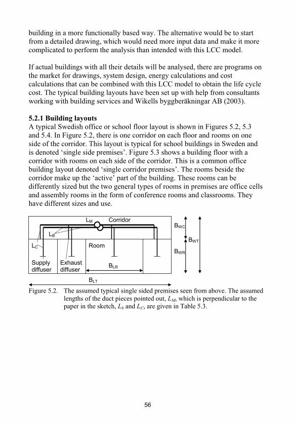
building in a more functionally based way. The alternative would be to start from a detailed drawing, which would need more input data and make it more complicated to perform the analysis than intended with this LCC model.

If actual buildings with all their details will be analysed, there are programs on the market for drawings, system design, energy calculations and cost calculations that can be combined with this LCC model to obtain the life cycle cost. The typical building layouts have been set up with help from consultants working with building services and Wikells byggberäkningar AB (2003).

5.2.1 Building layouts

A typical Swedish office or school floor layout is shown in Figures 5.2, 5.3 and 5.4. In Figure 5.2, there is one corridor on each floor and rooms on one side of the corridor. This layout is typical for school buildings in Sweden and is denoted ‘single side premises’. Figure 5.3 shows a building floor with a corridor with rooms on each side of the corridor. This is a common office building layout denoted ‘single corridor premises’. The rooms beside the corridor make up the ‘active’ part of the building. These rooms can be differently sized but the two general types of rooms in premises are office cells and assembly rooms in the form of conference rooms and classrooms. They have different sizes and use.

LC

LB

BLT

BWC

BWR

BWT

BLRSupply diffuser

Exhaust diffuser

LM

Room

Corridor

Figure 5.2. The assumed typical single sided premises seen from above. The assumed lengths of the duct pieces pointed out, LM, which is perpendicular to the paper in the sketch, Lb and LC, are given in Table 5.3.

56

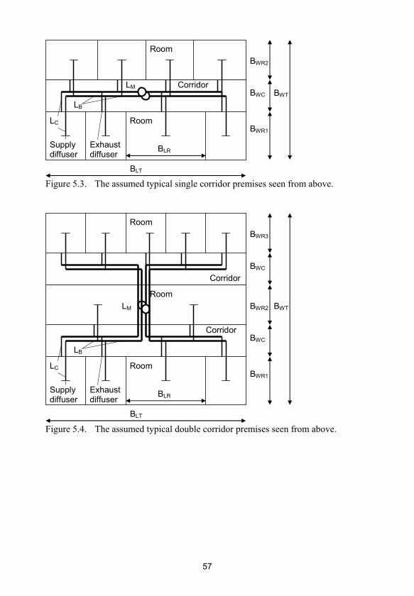
LC

LB

BLT

BWC

BWR1

BWT

BLRSupply diffuser

Exhaustdiffuser

LM

Room

Corridor

BWR2

Room

Figure 5.3. The assumed typical single corridor premises seen from above.

LC

LB

BLT

BWC

BWR1

BWT

BLRSupply diffuser

Exhaustdiffuser

Room

Corridor

BWR2

Room

BWC

BWR3

LM

Corridor

Room

Figure 5.4. The assumed typical double corridor premises seen from above.

57

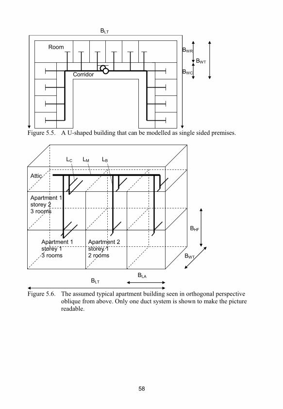
BLT

BWC

BWR

BWT

Room

Corridor

Figure 5.5. A U-shaped building that can be modelled as single sided premises.

BWT

BLT

Apartment 1 storey 1 3 rooms

Apartment 2 storey 1 2 rooms

Apartment 1 storey 2 3 rooms

Attic

LM LBLC

BLA

BHF

Figure 5.6. The assumed typical apartment building seen in orthogonal perspective oblique from above. Only one duct system is shown to make the picture readable.

58

BLT

LM

LB

LCBHF

BWT

Figure 5.7. The assumed typical detached house seen in orthogonal perspective oblique from above. Only one duct system is shown to make the picture readable.

In Figure 5.4, a floor layout with two corridors is shown. In between the corridors, there are usually conference rooms. Rooms, for example office cells, are located on the envelope side of the corridors. This type of layout is denoted ‘double corridor premises’.

In the LCC model, these three layouts are used to represent premises. Each room is assumed to have supply air. Exhaust air can be taken from each room or from the corridor on each storey. In the figures of the layouts, the buildings are straight but they can also form bends, circles or other curves as long as they are meant to have windows in each room. Figure 5.5 shows a single side premises based on the basic layout with exhaust air from the corridor on each floor. Many premises can be represented with this approach although more complicated buildings can be difficult to represent with this LCC model. Toilets, wardrobes and other such rooms have not been modelled to simplify the need for input data. The difference in costs for such parts caused by the choice of indoor climate system should be small.

Apartment buildings are assumed to have the same layout on all storeys. In this LCC model, the apartments are spread out as slices along the width of the building and the length corresponding to the apartment area. Inside the apartment, there are a number of rooms depending on the apartment size. Figure 5.6 shows this layout. The rooms with supply devices are the rooms that are not kitchens or bathrooms. Their number is nrsupply. Exhaust devices are located in the kitchen and in the bathrooms. Rooms with exhaust devices are not assumed to have any supply diffusers or air inlets. The number of exhaust devices is assumed to be two if nrsupply is three or less. The number of

59

exhaust devices is assumed to be three if nrsupply is above three, which is commonly associated with two bathrooms.

Detached houses are supposed to have one, two or three storeys, which represents most of the detached houses in Sweden. The rooms with supply devices are the rooms that are not kitchens, bathrooms, toilets or wardrobes. These rooms have supply diffusers or air inlets. Bathrooms, toilets, laundry rooms, kitchens and wardrobes have exhaust air. Table 5.1 gives the assumed room allocation for detached houses based on a detached house manufacturer (LB-Hus, 2005). Figure 5.7 shows the typical detached house.

Table 5.1. Assumed number of supply devices, nrfsupply, and exhaust devices, nrfexhaust, on the different storeys for detached houses. The thick-line divided columns are chosen based on the number of storeys in the house. The number of rooms with supply devices is nrsupply. The number of supply devices is given for the first storey under ‘s 1’, for the second storey under ‘s 2’ and for the third storey under ‘s 3’. The number of exhaust devices is given similarly as ‘e 1’, ‘e 2’ and ‘e 3’ respectively. For example, if there are five rooms with supply devices and the house is a two storey house, the bottom storey is assumed to have two supply devices and three exhaust devices. The second storey is assumed to have three supply devices and two exhaust devices.

nrsupply s 1 e 1 s 1 e 1 s 2 e 2 s 1 e 1 s 2 e 2 s 3 e 3

1 1 3 - - - - - - - - - -

2 2 3 1 2 1 1 - - - - - -

3 3 3 1 2 2 1 1 2 1 1 1 1

4 4 5 2 3 2 2 1 2 1 2 2 1

5 5 5 2 3 3 2 1 2 2 2 2 1

6 6 5 3 3 3 2 2 2 2 2 2 1

7 7 5 3 3 4 2 2 2 2 2 3 1

1 storey 2 storeys 3 storeys

The rooms can be differently sized for each of the four modelled zones. A typical school could be a single sided premises based building with a lot of classrooms and some office cells. A typical office building could be a single corridor building with a lot of office cells and two conference rooms. Different floors can have different layouts for premises. An interesting question is which size a building should have to make it beneficial to split the indoor climate system into two separate systems. That is possible to test by modelling half of a building and then doubling the result.

60

5.2.2 Requirements on the indoor climate

It could have been possible to try to value the benefit for obtaining the correct indoor climate or the cost for not. More and more results are coming out regarding health effects and productivity effects from the airflow rate, indoor air quality and temperature. Still, the results should be handled with caution when they are interpreted. Therefore, this LCC model assumes that the indoor climate system must accomplish correct indoor temperatures and a sufficient outdoor airflow rate. The form of requirements according to the Swedish building code (Boverket, 2002) has been used in the LCC model with a feature to insert airflow rate and temperature dependant costs. The principle requirements are expressed in l/(s·m²) and in l/(s·person). Enberg (1995) interpreted the recommended flow rate for dwellings to be 0.35 l/(s·m²) and for schools and offices to be 0.35 l/(s·m²) + 7 l/(s·person). The LCC model uses an airflow rate per floor area plus an airflow rate per person. The figures can be altered by the user of the LCC model. Concannon (2002) gives required airflow rates for a number of different countries.

5.2.3 Indoor climate systems

The indoor climate system is a subset of the building services. In a particular real or virtual building, different indoor climate systems can be used to solve the same problem of providing a good indoor climate. To compare different systems in a fair way, the same requirements must be used for all systems. In this paper, the indoor climate system consists of heating, ventilation and cooling system. Lighting is excluded and the plants supplying heating and cooling from primary fuels or electricity are not analyzed. Figure 5.8 shows the indoor climate system together with supporting systems and other building services. Most of the subdivisions are from Nilsson (2003b).

61

Lighting Electrical Other

Water Heating Cooling system system building

Air Air distri- plant plant services

distribu- treatment buted

tion system heating

system and

cooling

Fans Heating Pumps Boilers Chillers Commu- Cold tap

coil nication water

Duct Pipes District District systems

systems Cooling heating cooling Hot tap

coil Radiators Control water

Air Heat systems

terminals Heat Chilled pump Seewage

recovery beams Electrical

Control supply Elevators

Filter Control

Rubbish

Control chute

Building services

Indoor climate system Plant system

Air handling system

Figure 5.8. Building services and their subdivisions. The continuous framed part is modelled on a more detailed level in this paper and the dashed framed part is modelled in a simple way. The text above the horizontal dashed line gives the subsystems while the text below the horizontal dashed line give examples of equipment that can be used. For example, the ‘Air distribution system’ is a subset of the ‘Air handling system’. One type of equipment in the ‘Air distribution system’ is ‘Air terminals’ that is a generic term for supply devices and exhaust devices.

Figure 5.8 gives subdivisions with a functional perspective based on the systems included in the LCC model. Figure 5.9 shows the alternative indoor climate systems included in the LCC model even if not all combinations are applicable. Only typical indoor climate system combinations used in Sweden are included in the LCC model. Nilsson (2003b) and ASHRAE (2003; 2004) gives a broad view of other systems and alternatives used over the world. Figure 5.9 gives a subdivision of the indoor climate system. It helps to split different parts of the system but does not tell which parts are needed or not.

The building in a typical Swedish climate needs ventilation, heating and cooling depending on the situation. Ventilation is always needed for health reasons as long as the building is used. Heating or cooling is supplied to the

62

building via the ventilation air. All needed heating or cooling can be supplied by the ventilation air. If not, there is a need for added heating or cooling by a supporting system to allow the building to be in power balance. A hydronic system is an alternative that, in the case of heating, can be replaced by electrical radiators. The supporting system to fulfil the power balance is denoted ‘support heating’ or ‘support cooling’ depending on the sign this balancing power has.

Support Support

Exhaust CAV heating cooling

(E) One flow Flow ad- Flow Hydrau- Passive

justment value nic beams

Dis- Mixing Two flows Flow Tempera- radiators

placement with mea- ture Active

Low Ceiling timer suring Electri- beams

speed diffusers Occu- cal

diffusers Constant pancy radiators Induc-

Active branch tion

beams pressure Active units

beams

Air inlets Induction

needed units Induc-

tion

Exhaust units

air

heat pump

possible

1 2 3 4 5 6 7 8

Air cooling possible

Variable

Heat recovery

main pressure

control possible

Indoor climate system

Air path

Supply and exhaust

rooms or corridors

(SE)

Airflow rate

VAV

Air movement

Exhaust air from

Figure 5.9. The different indoor climate systems included in the LCC model categorized into subdivisions. ‘CAV’ means constant airflow rate. ‘VAV’ means variable airflow rate. Comments are made in text based on the numbers 1-8. For example, the ‘Air path’ can be ‘Supply and exhaust’ with a mixing ‘Air movement’ in the building. In that case, the LCC model includes three different alternative supply diffusers, namely ’Ceiling diffusers’, ‘Active beams’ and ‘Induction units’. If it is an office, the exhaust air can be taken from the rooms or from the corridors on each storey. It is possible to cool the supply air and heat recovery is possible.

To obtain an indoor climate system, an air path must be combined with an airflow rate approach and might be combined with a support heating system and a support cooling system. In this LCC model, it is assumed that a support heating system is always needed. For the air path, either exhaust air or supply

63

and exhaust air is used. In the case of exhaust air, an exhaust air heat pump can be added. In the case of supply and exhaust air, four different diffusers and two different locations for the exhaust devices are available. That means that for the air path subdivision, there are ten alternatives.

The airflow-rate subdivision contains two alternatives with constant airflow rate. For variable airflow rate, there are two alternatives for measuring the airflow rate in the rooms. They can be combined with two different kinds of room sensors to set the airflow rate. These two sensor techniques, occupancy and temperature, can be combined which gives three alternatives. All alternatives can either have a variable main pressure control or not. In total, the airflow rate subdivision contains 14 alternatives.

The support-heating subdivision contains four alternative solutions that are included in the LCC model. The support-cooling subdivision contains three alternatives. If the subdivisions for air path, airflow rate, support heating and support cooling are combined, it ends up with 10·14·4·3 = 1680 different indoor climate systems. Besides, the LCC model includes the possibility to have two duct design methods which double the number of alternatives. Nevertheless, a number of combinations are unrealistic or impracticable for certain buildings. Some comments need to be made based on the columns numbered 1-8 in Figure 5.9.

1. Exhaust ventilation is common in dwellings (SCB, 2003) and is usually of the CAV type even though VAV would be possible. It is possible to add an exhaust air heat pump to supply heat to tap water and water distributed heating. In premises, exhaust ventilation is uncommon. The air is supplied by air inlets, usually below or above the windows. In the case of an office building with an exhaust ventilation system, exhaust devices must be used in every room, not only in the corridors on each storey. Active beams or induction units are unfeasible since they include a supply diffuser. Cooling must be provided by passive beams among the modelled systems in Figure 5.9.

2. Supply and exhaust ventilation is common in premises. It exists in dwellings but is not common. If low speed diffusers are used, they are placed at the floor level and are not used in combination with active beams or induction units. In assembly rooms and rooms with a lot of people, low speed diffusers can be used to provide displacement ventilation. In offices, the exhaust air can be taken from every room or from the corridor on each storey.

3. Supply and exhaust ventilation with high speed diffusers are used to mix the air in the room. In the LCC model, the air can be supplied by ceiling diffusers,

64

active beams in the ceiling or induction units below the windows. Active beams and induction units induce room air through the diffuser and mix it with the outdoor air to increase the cooling capacity. Ceiling diffusers can be combined with passive beams. Active beams are not combined with induction units or passive beams in any combination.

4. Constant airflow rate is the most common airflow rate principle. A timer can be used to get a two level airflow rate which is still referred to as CAV.

5. Variable airflow rate, in this LCC model, can be adjusted by two methods. One is that a measuring device based on dynamic pressure controls a damper to a desired airflow rate. In that case, the main pressure after the air handling unit is constant. The other method is to control the branch pressure to be constant and adjust the diffuser outlet area to get a certain airflow rate. The idea with the second approach is that each branch damper opening is used to set the main pressure so the most open damper is almost fully open. An advantage with the second approach, not modelled, is that CAV and VAV diffusers can be used on the same branch since the branch pressure is constant.

6. The variable airflow rate can be set to give either appropriate amount of cooling power to the room at a certain supply air temperature or fresh air in the needed amount depending on the occupancy of the room or both. The occupancy controlled system is often called demand controlled ventilation (DCV). If temperature control is used, the VAV system is not combined with support cooling since the cooling is supposed to come from the air. An air heating system with VAV approach is not included in the LCC model. VAV diffusers must be ceiling diffusers or low speed diffusers.

7. A support heating system is assumed to be needed in every case to avoid low temperatures.

8. A support cooling system should be excluded in combination with a VAV system controlled by indoor temperature and can be excluded if cooling is not desired.

All systems included are centralized. Room air chillers or apartment air handling units are examples of decentralized systems (Yang et al., 2001; Zinn and Stigsson, 1993) that are not included in the LCC model.

5.2.4 Air terminals

The modelled diffusers are ceiling diffusers, active beams, induction units, low velocity diffusers and exhaust devices. Air inlets are used for supply air for

65

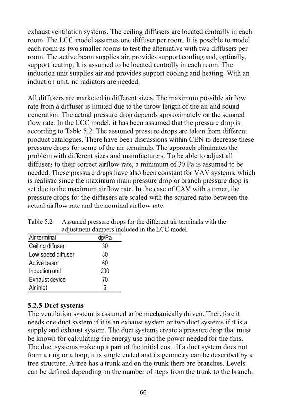
exhaust ventilation systems. The ceiling diffusers are located centrally in each room. The LCC model assumes one diffuser per room. It is possible to model each room as two smaller rooms to test the alternative with two diffusers per room. The active beam supplies air, provides support cooling and, optinally, support heating. It is assumed to be located centrally in each room. The induction unit supplies air and provides support cooling and heating. With an induction unit, no radiators are needed.

All diffusers are marketed in different sizes. The maximum possible airflow rate from a diffuser is limited due to the throw length of the air and sound generation. The actual pressure drop depends approximately on the squared flow rate. In the LCC model, it has been assumed that the pressure drop is according to Table 5.2. The assumed pressure drops are taken from different product catalogues. There have been discussions within CEN to decrease these pressure drops for some of the air terminals. The approach eliminates the problem with different sizes and manufacturers. To be able to adjust all diffusers to their correct airflow rate, a minimum of 30 Pa is assumed to be needed. These pressure drops have also been constant for VAV systems, which is realistic since the maximum main pressure drop or branch pressure drop is set due to the maximum airflow rate. In the case of CAV with a timer, the pressure drops for the diffusers are scaled with the squared ratio between the actual airflow rate and the nominal airflow rate.

Table 5.2. Assumed pressure drops for the different air terminals with the adjustment dampers included in the LCC model.

Air terminal dp/Pa

Ceiling diffuser 30

Low speed diffuser 30

Active beam 60

Induction unit 200

Exhaust device 70

Air inlet 5

5.2.5 Duct systems

The ventilation system is assumed to be mechanically driven. Therefore it needs one duct system if it is an exhaust system or two duct systems if it is a supply and exhaust system. The duct systems create a pressure drop that must be known for calculating the energy use and the power needed for the fans. The duct systems make up a part of the initial cost. If a duct system does not form a ring or a loop, it is single ended and its geometry can be described by a tree structure. A tree has a trunk and on the trunk there are branches. Levels can be defined depending on the number of steps from the trunk to the branch.

66

For a ventilation system, the main duct from the air handling unit has the first level. Branches on the main duct have the second level. Branches on the branches on the main duct have the third level and so on.

In this LCC model, three level branched duct systems are assumed. That means that highly complex buildings with more than three levels in the duct system are not modelled. An approach to pass this could be to use the LCC model to calculate the house in parts and finally calculate the entire building by letting each corridor be a super room based on the first calculations.

The assumed three level duct systems are shown in Figures 5.2-5.7 for the typical buildings. The highest level is called the main duct, the next level is called branch duct and the lowest level is called connection duct. For the supply duct system in typical premises, it is assumed that the main duct is located vertically in a shaft in the centre of the building with the air handling unit at the attic. For single sided and single corridor premises, each storey is supposed to have two branches. In double corridor premises, each storey is supposed to have four branches. The branches are supposed to be located in the false ceiling in the corridors. Every room is modelled with a connection duct and a diffuser between the branch and the centre of the room.

The exhaust duct system could have two different layouts, one with exhaust air in every room and one with exhaust air from each corridor on each storey. If air is extracted from every room, the system is modelled similarly to the supply duct system with the exception that the exhaust device is located at the wall towards the corridor. If air is extracted from each corridor, it is assumed that there is one branch per storey with one connection duct that extracts the supplied air on that storey. If there is no mechanical supply, there must be an exhaust device in each room.

In apartment buildings, the main duct is assumed to be located horizontally in the attic with the air handling unit on one end of the building. Each apartment needs one branch with silencers for the exhaust and for the supply duct systems respectively. Each room in each apartment has connection ducts and diffusers based on the width of the building according to Table 5.3.

In detached houses, a main duct is assumed to be installed vertically between the floors. Each floor needs a branch duct with connection ducts to each room. The layout and lengths of the modelled duct systems are shown in Figures 5.2-5.7 and Table 5.3.

67

Table 5.3. Assumed duct lengths in m for the typical buildings. Duct piece Premises Apartment buildings Detached houses

LM

2 m for the first piece

BHF between storeys

0 on the same storey

Distance between gable and

apartment centre for first piece

Distance between apartment

centres for rest

1 m for first piece

BHF for the rest

LB first

piece on

branch

Distance between

building centre and

nearest room centre +

BWC/2 + BWR/2

Storey number · BHF + 1 m

LB other

pieces

Distance between two

adjacent room centres0

LC supply BWC/2 + BWR/2 BWT/4 BWT/4

LC exhaust BWC/2 BWT/6 BWT/4

LM BHF - -

LB BWR/2 - -

LC 1 - -

Exhaust in each corridor

Supply: BLT/nrfsupply

Exhaust: BLT/(2·nrffexhaust)

The diameters of the duct pieces are designed by the LCC model. The LCC model uses a maximum constant pressure drop per length, R, for ducts since that method is wide spread (Nilsson, 2003b; Jensen, 2000), easy to use and gives a duct life cycle cost near the lowest possible by optimising R. The appended Paper V analyses this approach. The duct sizes used in Sweden approximately follow a Renard series where the ratio between two adjacent sizes is 100.1.

Alternatively, a maximum R can be inserted to the LCC model based on the first duct piece on each level of the duct systems. Then, the rest of the duct pieces on that level are assumed to have the same diameter as the first piece. This method is also analyzed in the appended Paper V. This is equivalent to constant branch diameters and should result in simpler logistic and mounting as well as better flexibility. None of these advantages are modelled since Wikells byggberäkningar AB (2003) do not list those kinds of benefits.

The resulting air speed as a function of R and the diameter, d, is given by Figure 5.10. An excessive air speed generates too much sound and should be avoided. Jagemar (1991) recommends a maximum air speed of 3 m/s for connection ducts, 5 m/s for branch ducts and 8 m/s for main ducts. The

68

optimal choice of R is a compromise between low pressure drop and low duct envelope surface which costs less. A certain R in a duct gives a lower air speed in smaller ducts than in larger ducts. The air speed at a certain R is proportional to the square root of the diameter. This is useful since the recommended air speed is lower for the smaller ducts closer to the rooms. If the connection duct is assumed to be 160 mm and the maximum air speed is 3 m/s, this corresponds to a maximum R of approximately 1 Pa/m.

In duct systems, there should be a number of diameters of duct before a non-duct component to make a correctly developed flow profile possible (Johansson and Svensson, 1998). In this LCC model, it is assumed that this is not a problem with the dimensions given by Table 5.3.

v / (m/s)

0

5

10

15

0 0.2 0.4 0.6 0.8 1

d / m

R=2 Pa/m

R=1 Pa/m

R=0.5 Pa/m

Figure 5.10. The air speed as a function of pressure drop per meter duct and duct diameter according to Equation 5.1 with an air density of 1.2 kg/m³.

The connection ducts for the typical buildings in this LCC model are assumed to be of the same size as the diffuser yields for a specific flow. It would be possible to insert two reductions to change the connection duct size but that should not be done in practice.

The other components belonging to the duct system are T-junctions, bends, reductions and adjusting dampers on each branch. These components create pressure drops. Jensen (1995) gives the pressure drop for these components according to Equation 5.1-5.6, which are used in the PFS program (Jensen, 1995). These pressure drops are used in the LCC model. For T-junctions, more equations are presented by Jensen (1995) for other flow directions but they are not used in this LCC model.

69

8541.4

8376.1

0158.0d

qLdp ductduct (5.1)

9.3

9.1

0025.0d

qdpbend (5.2)

313 3600.02392.04212.0( vvdpTs

)1950.03192.01583.0 2331

21 vvvv (5.3)

212 0650.00433.01983.0( vvdpTs

)1392.01433.04475.0 2221

21 vvvv (5.4)

with v1 v2 v3

313 0292.01133.04075.0( vvdpTe

)3492.05250.02775.0 2331

21 vvvv (5.5)

212 3183.05175.02342.0( vvdpTe

)4325.06208.01658.0 2221

21 vvvv (5.6)

withv1 v2 v3

Silencers are assumed to not have more pressure drop than an equivalent piece of duct. It is assumed that the connection duct length is same for all supply diffusers. The ceiling mounted diffuser is assumed to be mounted in the centre of the room. The low speed diffuser for displacement ventilation needs ducts from the ceiling to the top of the diffuser. It is usually located at the wall close to the corridor, which, for normally sized rooms, needs the same length of connection ducts. The active chilled beam is usually mounted centrally as the ceiling diffuser. The induction coil is assumed to be supplied with air from a branch located in the corridor. The connection duct usually supplies two induction coils in two adjacent rooms. That eliminates every second connection duct but needs the entire room length for the remaining connection ducts. In wide rooms, it can be preferable to have one connection duct for each induction unit but nothing prevents the builder from doing so. Therefore, ducts

70

for induction coils were modelled in the same way as the other types of supply diffusers.

5.2.6 Pipe systems

Pipe systems are used in hydronic heating or cooling systems. Examples of hydronic heating and cooling systems include induction coils, active or passive chilled beams and hydronic radiators. In the LCC model, the pump energy for the hydronic pumps is assumed to be zero. This simplification is based on the fact that water carries more energy than air does per volume flow rate. The higher water density than air density is combined with a possible higher temperature difference between incoming and outgoing medium. For example, cooling provided by air can be done with a temperature difference between the air and the room of 8°C. A typical temperature difference of a hydronic cooling system can be 10°C. For a hydronic heating system it can be 10°C but it can also be much higher.

A way to test the simplification of neglecting the pipe system pressure drop is to express the ratio between the energy for moving the medium and the carried energy. A certain cooling power from air, described by Equation 5.7, gives the needed airflow rate, q. Equation 5.8 gives the needed fan power at that airflow rate where fan is approximated to 50%. A typical total pressure drop for a ventilation system is 600 Pa. In combination, the airflow rate is shortened, resulting in Equation 5.9, which gives the ratio between fan power and cooling power. With typical figures on and cp, this ratio becomes 12%. Here, it is assumed that the fan power must not be cooled.

tqcP paircool (5.7)

fan

fan

dpqP (5.8)

%12810082.15.0

600

tc

dp

P

P

pfanaircool

fan (5.9)

The same equations can be used regarding the hydronic system with the use of water density and heat capacity of water instead of air. Equation 5.10 gives the ratio between the pump power and the cooling power with typical figures. The pump efficiency is assumed to 20%, the temperature difference to 10°C and the typical pressure drop in the hydronic system to 100 kPa. The ratio between the pump power and the cooling power becomes 1.2%.

71

%2.110418010002.0

100000

tc

dp

P

P

wpumpwatercool

pump (5.10)

The conclusion from that example is that the pressure drop in the pipe systems is of small importance. Another conclusion is that for the duct system design, it is reasonable to simplify the pressure drop calculation as done in the LCC model. The main purpose with modelling the pipe systems is to estimate their installation costs and repair costs.

Water pipes are always in pairs for supply and return in two pipe systems that are the common system in new buildings. Table 5.4 gives the length of each pipe level for the modelled buildings if pipe systems are needed. Stack pipes are vertical and distribution pipes are horizontal. The water pipe system can be organized in three levels, as with ducts, called stack pipes, distribution pipes and connection pipes. Connection pipes make up the piece between the hydronic heater or cooler and the rest of the pipe system.

In premises, distribution pipes are the second level when compared to a tree structure. They are usually located in the corridor’s false ceiling and connected to the radiator system (Wikells byggberäkningar AB, 2005). Heating distribution pipes usually supply three floors while cooling distribution pipes supply only one floor. Stack pipes are the highest level in the tree structure. They supply the distribution pipes if there are more than three floors in the heating case or one floor in the cooling case.

In apartment buildings, the distribution pipes have the highest level. The distribution pipes go around the building perimeter. For each one-room apartment it is assumed that one stack pipe goes from bottom to top to supply the different connection’s pipes and radiators. For apartments with more than one room, nrsupply >1, two stack pipes are assumed. Stack pipes therefore have the second level.

In detached houses, it is assumed that a distribution pipe exists along the perimeter of the house with connection pipes to each radiator. No stack pipes are used in this case.

72

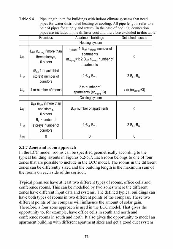
Table 5.4. Pipe length in m for buildings with indoor climate systems that need pipes for water distributed heating or cooling. All pipe lengths refer to a pair of pipes for supply and return. In the case of cooling, connection pipes are included in the diffuser cost and therefore excluded in this table. Premises Apartment buildings Detached houses

LPS

BHF·nstorey if more than

three storeys,

0 others

nrsupply=1: BHF·nstorey·number of

apartments

nrsupply>1: 2·BHF·nstorey·number of

apartments

0

LPD

(BLT for each third

storey)·number of

corridors

2·BLT·BWT 2·BLT·BWT

LPC 4 m·number of rooms2 m·number of

apartments·(nrsupply+3)2 m·(nrsupply+3)

LPS

BHF·nfloor if more than

one storey,

0 others

BHF·number of apartments 0

LPD

BLT·number of

storeys·number of

corridors

2·BLT·BWT 2·BLT·BWT

LPC 0 0 0

Heating system

Cooling system

5.2.7 Zone and room approach

In the LCC model, rooms can be specified geometrically according to the typical building layouts in Figures 5.2-5.7. Each room belongs to one of four zones that are possible to include in the LCC model. The rooms in the different zones can be differently sized and the building length is the maximum sum of the rooms on each side of the corridor.

Typical premises have at least two different types of rooms, office cells and conference rooms. This can be modelled by two zones where the different zones have different input data and systems. The defined typical buildings can have both types of rooms in two different points of the compass. These two different points of the compass will influence the amount of solar gain. Therefore, a four zone approach is used in the LCC model. That gives the opportunity to, for example, have office cells in south and north and conference rooms in south and north. It also gives the opportunity to model an apartment building with different apartment sizes and get a good duct system

73

calculation based on the different airflow rates for the different apartments. For detached houses, a one zone approach is adopted to avoid the discussion of the border between the zones.

All four zones have the air handling unit in common. The duct system and its pressure level are also the same for the four zones. Therefore, a choice must be made between ceiling or low speed diffusers, active beams and induction units for all zones since they have different pressure drops. The LCC model assumes that the choice of exhaust device for each room or for each corridor is in common for all four zones to simplify the duct system layout. An optional heat pump or heat recovery works with the entire system. The constant or variable airflow rate is also chosen for all zones together.

A number of data regarding for example occupancy, airflow rates and support heating and cooling systems can be different for each zone. No flow of air or energy is modelled between the zones. It is reasonable since different zones are meant to represent different kinds of rooms. A more detailed model could use one zone per room but that would need expressions for the flow of air and energy between the rooms that incorporates a lot of data about the behaviour of the building user.

5.3 Initial costs

The initial cost is defined as the cost that occurs in the beginning of the life cycle, at time zero. The terms installation cost or first cost are also used in literature. The initial cost consists of the cost for material for the indoor climate system components and the labour cost for mounting them. That incorporates duct system components, air terminals, air handling unit, fire dampers, silencers, control equipment, water pipe system, support heating and cooling components and adjustment of duct systems and pipe systems. It is also possible to input the costs for electrical, heating and cooling plants into the LCC model.

To be able to find costs for all components, the indoor climate system components must be dimensioned, which is described in the section regarding energy costs. This is due to the fact that component costs are usually a function of the size of the component and the size of the component is a function of the power it should generate or the airflow rate it should provide. Since this paper focuses on Swedish conditions, costs in Sweden have been used. The approach should be possible to use in other countries but the figures need to be changed. Wikells byggberäkningar AB (2003) has cost databases for the building industry based on empirical data. They present costs including labour for different components and systems for buildings. One of the databases deals

74

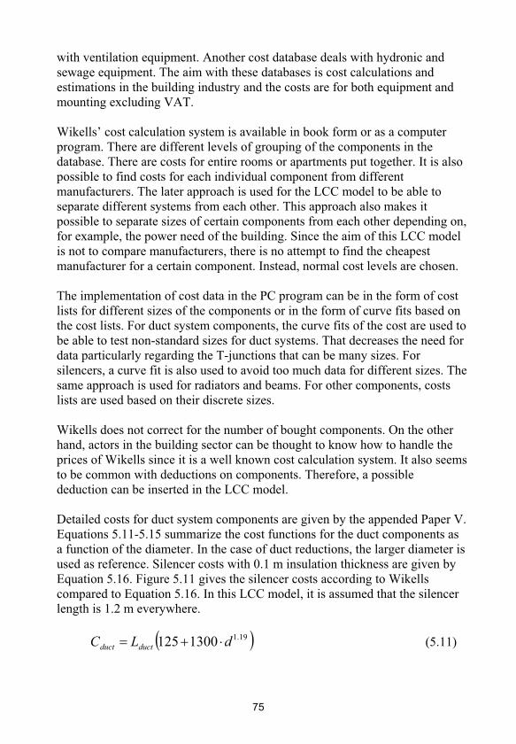
with ventilation equipment. Another cost database deals with hydronic and sewage equipment. The aim with these databases is cost calculations and estimations in the building industry and the costs are for both equipment and mounting excluding VAT.

Wikells’ cost calculation system is available in book form or as a computer program. There are different levels of grouping of the components in the database. There are costs for entire rooms or apartments put together. It is also possible to find costs for each individual component from different manufacturers. The later approach is used for the LCC model to be able to separate different systems from each other. This approach also makes it possible to separate sizes of certain components from each other depending on, for example, the power need of the building. Since the aim of this LCC model is not to compare manufacturers, there is no attempt to find the cheapest manufacturer for a certain component. Instead, normal cost levels are chosen.

The implementation of cost data in the PC program can be in the form of cost lists for different sizes of the components or in the form of curve fits based on the cost lists. For duct system components, the curve fits of the cost are used to be able to test non-standard sizes for duct systems. That decreases the need for data particularly regarding the T-junctions that can be many sizes. For silencers, a curve fit is also used to avoid too much data for different sizes. The same approach is used for radiators and beams. For other components, costs lists are used based on their discrete sizes.

Wikells does not correct for the number of bought components. On the other hand, actors in the building sector can be thought to know how to handle the prices of Wikells since it is a well known cost calculation system. It also seems to be common with deductions on components. Therefore, a possible deduction can be inserted in the LCC model.

Detailed costs for duct system components are given by the appended Paper V. Equations 5.11-5.15 summarize the cost functions for the duct components as a function of the diameter. In the case of duct reductions, the larger diameter is used as reference. Silencer costs with 0.1 m insulation thickness are given by Equation 5.16. Figure 5.11 gives the silencer costs according to Wikells compared to Equation 5.16. In this LCC model, it is assumed that the silencer length is 1.2 m everywhere.

19.11300125 dLC ductduct (5.11)

75

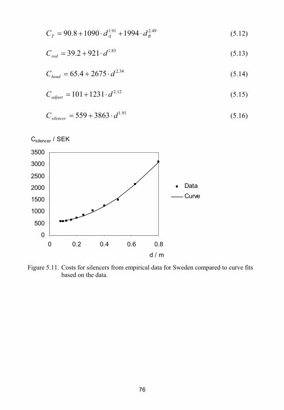
49.291.1 199410908.90 BAT ddC (5.12)

83.19212.39 dCred (5.13)

34.226754.65 dCbend (5.14)

12.21231101 dCadjust (5.15)

91.13863559 dCsilencer (5.16)

Csilencer / SEK

0

500

1000

1500

2000

2500

3000

3500

0 0.2 0.4 0.6 0.8

d / m

Data

Curve

Figure 5.11. Costs for silencers from empirical data for Sweden compared to curve fits based on the data.

76

Table 5.5-5.7 gives the listed costs for different components. For exhaust air heat pumps and air handling units, costs were collected from manufacturers since Wikells does not include them. Curve fits are given for many of the components as a function of size. If these functions are close to linear, a linear curve fit is given. If they are far from linear, an exponent is added to the size parameter. In many cases, it is possible to describe the cost of a component linearly with an added constant. That means that it is better to have one large component than two small components since there will be only one constant added.

If the largest size of a component is not enough, the assumed approach is to add a sufficient number of the largest item to match the needed airflow rate or power. For example, the largest exhaust device handles 200 l/s only. If 600 l/s is needed for a corridor, three such devices can be used. Some extra duct components are needed but it is most likely that the number of devices would give some deduction to compensate the extra duct pieces. Usually, the largest component is enough in a certain case but if not, the size does still influence the total cost in a reasonable way.

77

Table 5.5. Assumed costs for components excluding VAT.

Connec-

tion, d/m

Flow,

q/(l/s)

Unit cost

/ SEK

Connec-

tion, d/m

Flow,

q/(l/s)

Unit cost

/ SEK

Connec-

tion, d/m

Flow,

q/(l/s)

Unit cost

/ SEK

Ceiling diffusers for Transfer units Ceiling diffusers for

dwellings Flow at 5 Pa drop constant branch

Flow at 25 dB(A) Used with exhaust in pressure control

0.080 11.5 195 corridor on each floor Flow at 25 dB(A)

0.100 17.5 198 0.6x0.1 27 698 No VAV damper needed

0.125 37 226 0.7x0.1 32 761 0.160 68 2522

0.160 60 267 0.8x0.1 35 796 0.200 100 2892

0.200 100 290 0.9x0.1 40 841 0.250 145 3114

Curve fit: 120 + 867·d 1.0x0.1 45 903 0.315 180 3387

Ceiling diffusers for Curve fit: 402 + 11.1·q Curve fit:

premises Air inlet -2261 + 7457·d0.237

Flow at 30 dB(A) One for each room Exhaust devices for

0.100 35 882 with supply constant branch

0.125 65 1042 - - 931 pressure control

0.160 75 1042 VAV damper Flow at 25 dB(A)

0.200 105 1375 Must be added to No VAV damper needed

0.250 120 1397 ceiling or low speed 0.160 33 2754

Curve fit: 548 + 3586·d diffusers and exhaust 0.200 55 3058

Low speed diffusers devices for VAV systems. 0.250 65 3286

Flow at 25 dB(A) 0.100 - 3881 0.315 95 3514

0.125 55 4569 0.125 - 3925 Curve fit: 1432 + 52.6·d0.642

0.160 85 4240 0.160 - 3976 Exhaust heat pump

0.200 135 4786 0.200 - 4158 Detached houses,

0.250 180 5546 0.250 - 4293 extra cost

0.315 300 6588 0.315 - 4465 - 150 10205

0.400 425 8342 0.400 - 4809 Apartment buildings,

0.500 625 13564 0.500 - 5283 premises

0.630 900 17643 Curve fit: - 300 54007

Curve fit: 3758 + 4507·d1.57

- 600 65607

3652 + 38977·d2.16

Fire damper - 900 89207

Exhaust devices Used between floors - 3000 128907

Flow at 25 dB(A) in premises Curve fit:

0.100 25 339 0.200 - 5439 -104953 + 45013·q0.209

0.125 35 357 0.400 - 6832

0.160 60 375 0.630 - 8845

0.200 80 422 Curve fit: 3783 + 7941·d

Curve fit: 255 + 807·d

78

Table 5.6. Assumed costs for components excluding VAT.

Connec-

tion, d/m

Flow,

q/(l/s)

Unit cost

/ SEK

Connec-

tion, d/m

Flow,

q/(l/s)

Unit cost

/ SEK

Connec-

tion, d/m

Flow,

q/(l/s)

Unit cost

/ SEK

Exhaust fan Air handling units Chilling coil - air

With connections Excluding chilling coil handling unit

and control Type 1 - 520 5000

Flow at 100 Pa raise Flow at 150 Pa raise - 760 8000

0.125 23 3242 0.125 68 12918 - 1400 10000

0.160 83 3474 0.160 86 19567 - 3500 15000

0.200 146 3737 0.160 115 20797 - 5300 20000

Curve fit: 3066 + 3.72·q 0.200 180 22033 - 6900 25000

Square connection Curve fit: 6251 + 774·q0.594

Curve fit: 4994 + 2.89·q

Hydraulic diameter Type 2

Flow at 150 Pa raise Flow at 200 Pa raise

0.329 164 8358 0.200 200 60508

0.347 308 10701 0.250 350 66578

0.425 602 11834 0.315 500 76660

0.469 870 12784 Curve fit: 49071 + 53.8·q

Flow at 200 Pa raise Type 3

0.532 1241 14687 Flow at 200 Pa raise

0.558 1500 15312 0.315 520 88815

0.594 1865 15252 0.400 760 97422

0.659 2453 22116 0.630 1400 131125

0.836 3784 26966 1.000 3500 186050

Curve fit: 8314 + 4.94·q 1.250 5300 280706

1.600 6900 337674

Curve fit: 68158 + 38.7·q

79

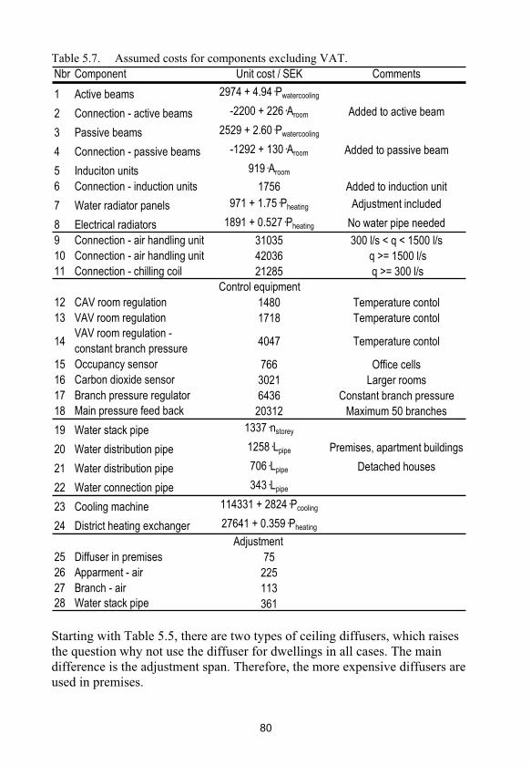
Table 5.7. Assumed costs for components excluding VAT. Nbr Component Unit cost / SEK Comments

1 Active beams 2974 + 4.94·Pwatercooling

2 Connection - active beams -2200 + 226·Aroom Added to active beam

3 Passive beams 2529 + 2.60·Pwatercooling

4 Connection - passive beams -1292 + 130·Aroom Added to passive beam

5 Induciton units 919·Aroom

6 Connection - induction units 1756 Added to induction unit

7 Water radiator panels 971 + 1.75·Pheating Adjustment included

8 Electrical radiators 1891 + 0.527·Pheating No water pipe needed

9 Connection - air handling unit 31035 300 l/s < q < 1500 l/s

10 Connection - air handling unit 42036 q >= 1500 l/s

11 Connection - chilling coil 21285 q >= 300 l/s

12 CAV room regulation 1480 Temperature contol

13 VAV room regulation 1718 Temperature contol

14VAV room regulation -

constant branch pressure4047 Temperature contol

15 Occupancy sensor 766 Office cells

16 Carbon dioxide sensor 3021 Larger rooms

17 Branch pressure regulator 6436 Constant branch pressure

18 Main pressure feed back 20312 Maximum 50 branches

19 Water stack pipe 1337·nstorey

20 Water distribution pipe 1258·Lpipe Premises, apartment buildings

21 Water distribution pipe 706·Lpipe Detached houses

22 Water connection pipe 343·Lpipe

23 Cooling machine 114331 + 2824·Pcooling

24 District heating exchanger 27641 + 0.359·Pheating

25 Diffuser in premises 75

26 Apparment - air 225

27 Branch - air 113

28 Water stack pipe 361

Adjustment

Control equipment

Starting with Table 5.5, there are two types of ceiling diffusers, which raises the question why not use the diffuser for dwellings in all cases. The main difference is the adjustment span. Therefore, the more expensive diffusers are used in premises.

80

Transfer units must be present if the air is extracted from the corridor and not from each room. Air inlets are used for every room with supply air if there is no mechanical supply system.

In VAV systems without constant branch pressure, a VAV damper is needed for supply and exhaust respectively. If constant branch pressure is used for a VAV ventilation system, certain diffusers must be used for supply and exhaust respectively. No VAV damper is needed in that case. Fire dampers are needed between each fire zone. Here, it is assumed that it means between each storey in premises.

For exhaust heat pumps in apartment buildings and premises, it is assumed that the heat plant system is located in the basement or first storey and the exhaust fan is on the roof or in the attic. Therefore, water pipes for 674 SEK/m is assumed for the building height plus 10 m for connection purposes. For exhaust heat pumps for detached houses, it is assumed that the exhaust air heat pump unit includes a boiler for hydronic heating and tap water heating. This boiler cost is subtracted from the exhaust air heat pump cost since it is needed anyway.

The air handling units are split into three groups depending on their size corresponding to different manufacturers. The first type is addressed to detached houses with a plate heat exchanger. The second type is Wikells’ typical air handling units with rather low airflow rates but higher than for detached houses. The third type includes larger units, which have rotating heat exchanger. All the air handling unit control is included. For the larger air handling units, the connections are rectangular. In these cases, the hydraulic diameter corresponding to the circular standard sizes is given.

All included air handling units have heat recovery. Heat recovery is highly efficient, which can be shown by expressing the ratio between the saved heating energy and the added fan electricity due to the added pressure drop from the heat recovery unit. Equation 5.17 gives the saved heat power for a heat recovery system with the temperature efficiency defined according to Equation 5.18. The extra fan power to overcome the added pressure drop is given by Equation 5.19. The ratio between the saved power and the added power due to the pressure drop is shown in Equation 5.20. Typical numbers are inserted for fan, hr and dphr = 400 Pa which refers to the pressure drop on both sides of the heat recovery unit and filter.

outinhrpsaved ttcqP _ (5.17)

81

outex

outinhrhr tt

tt _ (5.18)

fan

hrfan

qdpP (5.19)

outexoutex

outex

hr

phrfan

fan

saved

tttt

ttdp

c

P

P

2.1400

10082.18.05.0 (5.20)

This ratio can be seen as the coefficient of performance for a heat recovery system. If the room temperature is assumed to be the same as the exhaust temperature, the outdoor temperature is assumed to be 6.7°C, which is normal annual average for Stockholm, and the indoor temperature is assumed to be 20°C, it results in a coefficient of performance of the heat recovery unit of 16.1. It means that, from the running perspective, the electricity price must be 16.1 times the heat price to make the heat recovery system unprofitable.

The power ratio expressed in Equation 5.20 can be integrated over time to give the ratio between annual energy savings and annual added energy due to the pressure drop increase in the heat recovery unit. The degree hours, based on the exhaust temperature as limit temperature and the outdoor temperature, can be expressed according to Equation 5.21. This equation can be combined with Equation 5.17 and 5.18 to give the saved energy during a year with heat recovery. It is assumed that the heat recovery is not used when the outdoor temperature exceeds the indoor temperature. It is assumed that the airflow rate, density of air, heat capacity of air and all efficiencies are constant. Equation 5.22 gives the ratio between the saved annual energy and the added annual fan energy to overcome the extra pressure drop of the heat recovery. The number of degree hours, Dh, is approximately 118000 for a normal year in Stockholm based on 20°C exhaust temperature. With the same typical numbers as in Equation 5.20, the ratio becomes 16.3.

8760

1, )0,max(

iioutex ttDh (5.21)

82

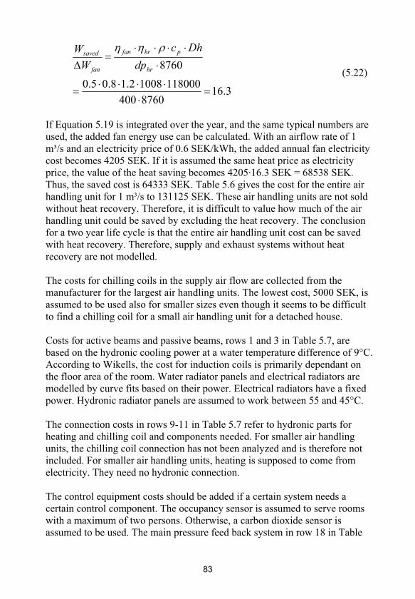
3.168760400

11800010082.18.05.0

8760hr

phrfan

fan

saved

dp

Dhc

W

W

(5.22)

If Equation 5.19 is integrated over the year, and the same typical numbers are used, the added fan energy use can be calculated. With an airflow rate of 1 m³/s and an electricity price of 0.6 SEK/kWh, the added annual fan electricity cost becomes 4205 SEK. If it is assumed the same heat price as electricity price, the value of the heat saving becomes 4205·16.3 SEK = 68538 SEK. Thus, the saved cost is 64333 SEK. Table 5.6 gives the cost for the entire air handling unit for 1 m³/s to 131125 SEK. These air handling units are not sold without heat recovery. Therefore, it is difficult to value how much of the air handling unit could be saved by excluding the heat recovery. The conclusion for a two year life cycle is that the entire air handling unit cost can be saved with heat recovery. Therefore, supply and exhaust systems without heat recovery are not modelled.

The costs for chilling coils in the supply air flow are collected from the manufacturer for the largest air handling units. The lowest cost, 5000 SEK, is assumed to be used also for smaller sizes even though it seems to be difficult to find a chilling coil for a small air handling unit for a detached house.

Costs for active beams and passive beams, rows 1 and 3 in Table 5.7, are based on the hydronic cooling power at a water temperature difference of 9°C. According to Wikells, the cost for induction coils is primarily dependant on the floor area of the room. Water radiator panels and electrical radiators are modelled by curve fits based on their power. Electrical radiators have a fixed power. Hydronic radiator panels are assumed to work between 55 and 45°C.

The connection costs in rows 9-11 in Table 5.7 refer to hydronic parts for heating and chilling coil and components needed. For smaller air handling units, the chilling coil connection has not been analyzed and is therefore not included. For smaller air handling units, heating is supposed to come from electricity. They need no hydronic connection.

The control equipment costs should be added if a certain system needs a certain control component. The occupancy sensor is assumed to serve rooms with a maximum of two persons. Otherwise, a carbon dioxide sensor is assumed to be used. The main pressure feed back system in row 18 in Table

83

5.7 is used together with the constant branch pressure VAV solution to be able to decrease the main pressure when possible.

The pipe costs are taken as an average from Wikell’s typical pipe costs for different buildings. There is no stratification into different sizes. Hydronic pipes can serve three floors for heating but only one floor for cooling.

Coarsely estimated costs for the heating and cooling plants are given by row 23 and 24 in Table 5.7. These costs are taken from Wikells but the curve fits are not the best since they contain a too large power span. Still, there is a clear power influence on the plant cost. Electrical supply cost was not collected. An electrical supply system is needed whether the building has an indoor climate system or not but the fuse size influences the cost. The LCC model has a feature to insert such data linearly depending on the power.

The adjustment costs are collected from Wikells byggberäkningar AB (2005). For CAV systems, adjustment is needed for both branches and diffusers. For VAV systems, the diffusers do not need adjustments. For VAV systems with constant branch pressure, the branches do not need adjusting. For dwellings, the adjustment was not varied with the flow rate principle.

In Table 5.7, most of the cost data is based on one or a few typical examples from Wikells byggberäkningar AB (2003). Hydronic radiator panel costs are based on 64 different sizes of actual radiator panels. The electrical radiator panel cost is from Wikells byggberäkningar AB (2004).

5.4 Energy costs and power need

The energy cost is usually a major part of the running costs. The energy cost originates from the energy use of electricity, heating and cooling. There is also a power related cost within the heating and cooling plant, the electrical installation and the needed components in the indoor climate system. Therefore, both maximum power need and annual energy use must be calculated by or inserted in the LCC model. This is included in this LCC model to be able to perform life cycle cost estimations without other programs.

The aim with calculating the energy use and power demand in the LCC model is to not only give a rough estimation of the energy use and the power demand but also to incorporate some unusual control strategies and parameters that are usually not included in other energy calculation programs.

The energy price is defined as the cost for 1 kWh of energy. It can be believed that the energy price will have a real price increase. Most likely, the difference

84

between electricity and heat will also increase, particularly in Sweden where the difference traditionally has been low but is increasing, se Figure 4.4 (Statens Energimyndighet, 2005; SCB, 2005). In 1986, in Sweden, electricity was 48% more expensive than district heating. In 2004, electricity was 106% more expensive for detached houses according to the statistics. Between 1998 and 2005, the real price change rate was on average 4.0% for electricity and 1.9% for district heating. The LCC model allows for different possible discount interest rates in the life cycle cost calculation for electricity, heat and other costs respectively. It is left to the user of the LCC model to obtain data on energy prices and discount interest rates.

The energy use is calculated by integrating the power balance for each hour of the year based on hourly outdoor climate data. An alternative would be to use duration curves (Nilsson, 1994) but the hourly approach is not a problem with modern computer speed. It gives the opportunity to directly model the thermal storage of the interior of the building. Figure 5.12 shows the room, the air handling unit (AHU) and the modelled powers with needed temperatures. The room must be in power balance according to Equation 5.23 and the air handling unit together with the plants must provide the balancing powers Psupport and Pvent. The terms of the power balance is discussed in EN ISO 13790:2003. The problem is to tell how much bought energy and maximum power is needed to supply the sufficient Psupport and Pvent to get the desired troom

and qvent. Equations 5.24-5.39 give the used expressions for the parameters shown in Figure 5.12. The ventilation system is assumed to be balanced. The temperature efficiency of the heat recovery unit (HRU) is given by Equation 5.18.

Psolar

Psupport

Pcap

Pvent

Pint

PleakPtrans

Pair

qleak

qleak

qvent

PHP_in Pfan_ex

qvent

Pfan_sa

PHP_gain

tsa

thr_in

tex

toutthr_out

HPtroom

HRU

ROOM

AHUtcap

Figure 5.12. The included powers in the power and energy calculation of the LCC model.

85

capventsolarintleaktranssupport PPPPPPP (5.23)

The control system and the actual response of indoor climate systems are not analyzed or modelled. It is assumed that neither support heating together withsupport cooling or air heating together with air cooling are used at the same time. That means that windows must be of good quality to avoid down draught when it is cold outdoors. It is also assumed that the room temperature actually is within in the given interval. Wen and Smith (2001) discuss an increase in energy use depending on time constants for thermostats. There are other programs that simulate the indoor climate system including control system (Equa, 2005).

The year is split into two groups of hours to simulate working time and non-working time which consists of nights and weekends. Different input data can be used for the two different time groups.

Equation 5.24 gives the transmitted heat based on Uav and the heat transmitting area to the outdoors, Atrans.

outroomtransavtrans ttAUP (5.24)

transleakleak Akq 05.0 for supply and exhaust system (5.25)

transleakleak Akq 01.0 for exhaust system (5.26)

Equations 5.25 and 5.26 give an estimation of the air leakage for low raise buildings due to wind and buoyancy. It is assumed that the heat transmitting area, Atrans, is the same as the leakage area. An exhaust system creates an under-pressure that eliminates a lot of the unintentional air leakage. The qvent

could be controlled to give a constant air change rate including unintentional air leakage but that is not done in practice. kleak should be measured according the standard SS 02 15 51. The leakage ratios, 1% and 5%, are annual average estimations. This is discussed in the appended Paper VII and by Torssell (2005). For example VIP+ (Strusoft, 2003) models actual leakage from wind and temperature data. Equation 5.27 gives the power for heating unintentional leakage air.

outroomleakpleak ttqcP (5.27)

The gained solar radiation in the building is described by Equation 5.28. The direct solar radiation, Pbeam, is taken from climate data as the power per m²

86

facing the sun. This power is scaled by cos( ) where is the angle between the normal to the window and the sun beam direction. This angle is calculated by the help of the sun azimuth and elevation. The windows can face different points of the compass but are assumed to be vertical. This means that half of the sky is seen by the window regarding the diffuse radiation.

The solar radiation transmittance depends on . In the LCC model, it is assumed that the transmittance, ksolar, is constant. That means that the solar radiation outside the window is scaled by ksolar to give the solar gain in the building. For a triple pane window with clear 3 mm glass panes, ksolar is typically 0.6 without solar shading (Källblad, 1998)

solardiffuse

beamwindowsolar kP

PAP2

cos (5.28)

Equation 5.29 gives the power from the supply air to the room. Equation 5.30 gives the power from the thermally active mass to the room. This power changes the temperature over time for the thermally active mass, tcap,according to Equation 5.31.

roomsaventpvent ttqcP (5.29)

roomcapcapcap ttAP 5.2 (5.30)

capcap

capcap

cm

Pt (5.31)

The number 2.5 in Equation 5.30 is the indoor heat transfer coefficient in W/(m²·K) on vertical surfaces according to the standard EN ISO 13791:2004. This simplification is used to avoid calculating every surface. tcap must be iterated hourly to avoid divergence. Acap is assumed to be the interior envelope area of the room. mcap is the mass inside the insulation of the interior envelope of the room. For the first hour of the year, an initial value of tcap is needed. The average of the desired temperature span is used.

The user of the LCC model sets the supply air temperature, tsa, which is assumed to be constant if there is a chilling coil. If chilling coil is not wanted, tsa follows the outdoor temperature if it is warmer outdoors than the desired tsa.In the case of variable airflow rate controlled by temperature, a maximum

87

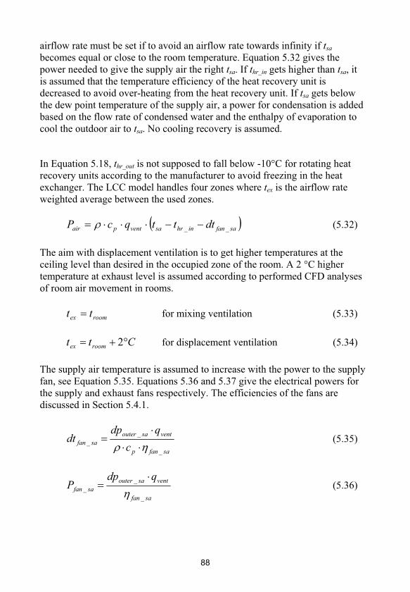
airflow rate must be set if to avoid an airflow rate towards infinity if tsa

becomes equal or close to the room temperature. Equation 5.32 gives the power needed to give the supply air the right tsa. If thr_in gets higher than tsa, it is assumed that the temperature efficiency of the heat recovery unit is decreased to avoid over-heating from the heat recovery unit. If tsa gets below the dew point temperature of the supply air, a power for condensation is added based on the flow rate of condensed water and the enthalpy of evaporation to cool the outdoor air to tsa. No cooling recovery is assumed.

In Equation 5.18, thr_out is not supposed to fall below -10°C for rotating heat recovery units according to the manufacturer to avoid freezing in the heat exchanger. The LCC model handles four zones where tex is the airflow rate weighted average between the used zones.

safaninhrsaventpair dtttqcP __ (5.32)

The aim with displacement ventilation is to get higher temperatures at the ceiling level than desired in the occupied zone of the room. A 2 °C higher temperature at exhaust level is assumed according to performed CFD analyses of room air movement in rooms.

roomex tt for mixing ventilation (5.33)

Ctt roomex 2 for displacement ventilation (5.34)

The supply air temperature is assumed to increase with the power to the supply fan, see Equation 5.35. Equations 5.36 and 5.37 give the electrical powers for the supply and exhaust fans respectively. The efficiencies of the fans are discussed in Section 5.4.1.

safanp

ventsaoutersafan

c

qdpdt

_

__ (5.35)

safan

ventsaoutersafan

qdpP

_

__ (5.36)

88

exfan

ventexouterexfan

qdpP

_

__ (5.37)

Equations 5.38 and 5.39 give the possible power gain from the exhaust air heat pump and the electrical input power to the compressor of the exhaust air heat pump. The exhaust air heat pump is assumed to chill the exhaust air to 5°C in dry conditions, which seems to be the practice according to the manufacturer (IVT, 2005; Nibe, 2005). The compressor power is constant resulting in an increasing outgoing air temperature if condensation occurs. The outgoing air temperature is not analysed to avoid a need for indoor vapour supply data. The gained heat from the exhaust heat pump, PHP_gain, can be used for heating tap water and hydronic radiators. The possible applicable ratio of PHP_gain that can be fed into these systems is set by the user of the LCC model. This ratio is assumed to be constant. The heating of hot tap water is not included in the LCC model. Therefore, the useful part of the gained heat from the exhaust air heat pump is subtracted from the support heating. It is assumed that tex>5 and COPHP>1.

51_ expvent

HP

HPgainHP tcq

COP

COPP (5.38)

51

1_ expvent

HP

inHP tcqCOP

P (5.39)

The ventilation airflow rate, qvent , and the internal power gain, Pint, need to be determined. The user of the LCC model sets a minimum qvent per floor area and per person respectively. For a CAV system, this airflow rate can be increased to handle cooling by air only. For a CAV system, a timer can be used to decrease the airflow rate to a lower level, corresponding to the airflow rate per floor area only, parts of the day and week. For a VAV system controlled by temperature, the minimum airflow rate is given by the requirements in the same way as for a CAV system. If cooling is needed, the airflow rate increases to provide the sufficient Pair.

For a VAV system controlled by occupancy, the airflow rate is linearly scaled between the airflow rate required per floor area and the airflow rate for both persons and floor area depending on the occupancy rate. The occupancy rate used is the average for the daytime and night time respectively. For a VAV system controlled by both temperature and occupancy, the approaches are combined.

89

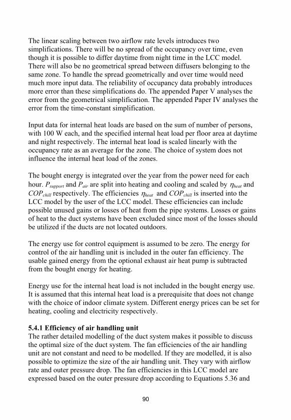
The linear scaling between two airflow rate levels introduces two simplifications. There will be no spread of the occupancy over time, even though it is possible to differ daytime from night time in the LCC model. There will also be no geometrical spread between diffusers belonging to the same zone. To handle the spread geometrically and over time would need much more input data. The reliability of occupancy data probably introduces more error than these simplifications do. The appended Paper V analyses the error from the geometrical simplification. The appended Paper IV analyses the error from the time-constant simplification.

Input data for internal heat loads are based on the sum of number of persons, with 100 W each, and the specified internal heat load per floor area at daytime and night respectively. The internal heat load is scaled linearly with the occupancy rate as an average for the zone. The choice of system does not influence the internal heat load of the zones.

The bought energy is integrated over the year from the power need for each hour. Psupport and Pair are split into heating and cooling and scaled by heat and COPchill respectively. The efficiencies heat and COPchill is inserted into the LCC model by the user of the LCC model. These efficiencies can include possible unused gains or losses of heat from the pipe systems. Losses or gains of heat to the duct systems have been excluded since most of the losses should be utilized if the ducts are not located outdoors.

The energy use for control equipment is assumed to be zero. The energy for control of the air handling unit is included in the outer fan efficiency. The usable gained energy from the optional exhaust air heat pump is subtracted from the bought energy for heating.

Energy use for the internal heat load is not included in the bought energy use. It is assumed that this internal heat load is a prerequisite that does not change with the choice of indoor climate system. Different energy prices can be set for heating, cooling and electricity respectively.

5.4.1 Efficiency of air handling unit

The rather detailed modelling of the duct system makes it possible to discuss the optimal size of the duct system. The fan efficiencies of the air handling unit are not constant and need to be modelled. If they are modelled, it is also possible to optimize the size of the air handling unit. They vary with airflow rate and outer pressure drop. The fan efficiencies in this LCC model are expressed based on the outer pressure drop according to Equations 5.36 and

90

5.37. By the use of the measured airflow rate, outer pressure drop and the active electrical input power, the outer fan efficiency can be obtained. These measurements have been performed by the manufacturers of the units. This makes the LCC model more realistic since the data comes from actual measurements of actual equipment. The disadvantage is that the construction of an air handling unit is never tested and optimised.

In this LCC model, curve fits are created for the outer fan efficiencies as function of the size of the connection to the unit, the airflow rate and the outer pressure drop where it is assumed that all dynamic pressure goes lost. The idea is to give a curve as simple as possible with the least square-error method. For fans, which are used in exhaust systems, it is reasonable to describe fan_ex as a second degree polynomial of L, se Equation 5.40. A theoretical fan has a constant efficiency for a constant L but that is not true in practice due to losses in outlet, motors and control equipment. On the other hand, it is reasonable to believe that fan_ex approaches an asymptote when the fan angular speed goes towards infinity. It is reasonable to believe that there is a maximum efficiency at a certain L. At higher or lower L, the efficiency should be lower. A second degree polynomial function fulfils that demand. To fit the curves to fans of different sizes and kinds, a fifth degree polynomial expression of the connection diameter is used.

ds

d

pp

pL 10 (5.40)

Equation 5.41 gives fan_ex for exhaust fans. Approximately 400 measured data from three actual fan sizes were used for the curve fit. Figure 5.13 gives the outer fan efficiency for exhaust fans as a function of the hydraulic diameter. If Equation 5.41 gives a fan_ex below zero, it is set to 2% to avoid zero denominators and unreasonable efficiencies. This function should also not be used at higher pressure drops than the fan actually manages. The maximum airflow rate a fan can give is assumed to be the listed airflow rate at the outer pressure drops according to Table 5.7.

)9.1915.4386.349

0.10775.6001192.0(

16.100422.3845.7

543

2

002508.02

__

AHUAHUAHU

AHUAHU

dp

exfan

ddd

dd

eL outerex

(5.41)

91

The standard deviation of the error between the curve fit and the measured points can express the quality of the given curve fits. For exhaust fans, this standard deviation is 2.8%. If the average efficiency were used instead of the equation, the standard deviation would be 14%.

f an_ex / %

0

20

40

60

0 0.2 0.4 0.6 0.8

dh / m

200 Pa

100 Pa

Figure 5.13. The outer fan efficiency for exhaust fans at L=3.4 at the outer pressure difference of 200 Pa and 100 Pa respectively.

For small air handling units with supply and exhaust with an airflow rate of up to 180 l/s, measurements have been available for both the exhaust and supply side respectively. For these units, there are a number of pressure drops inside the unit. These are partly linear and partly squared. Therefore, it is better to describe the outer fan efficiency as function of the average speed in the outlet instead of L.

Equations 5.42 and 5.43 give the outer efficiencies based on measurements from two different sizes of air handling units, including 60 data. Also here, a 2 % lower limit was used. The standard deviation of the error is 0.78% for the supply side and 0.82% exhaust side. The standard deviation of the measured data, which is the same as if the average were used, is 4.8% and 5.7% respectively for supply and exhaust.

exouter

AHU

dp

dexfan

e

ev

_003053.0

63.132

_

1

191.37656.4400.1 (5.42)

92

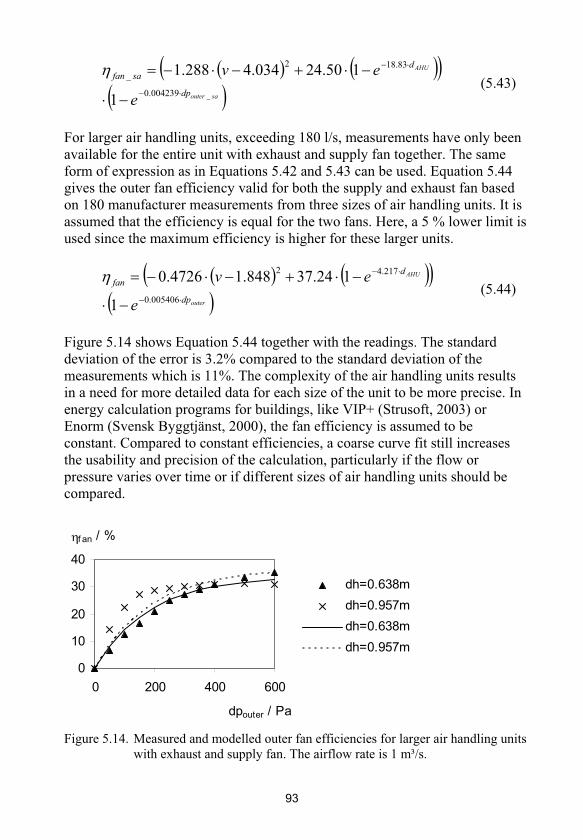
saouter

AHU

dp

dsafan

e

ev

_004239.0

83.182

_

1

150.24034.4288.1 (5.43)

For larger air handling units, exceeding 180 l/s, measurements have only been available for the entire unit with exhaust and supply fan together. The same form of expression as in Equations 5.42 and 5.43 can be used. Equation 5.44 gives the outer fan efficiency valid for both the supply and exhaust fan based on 180 manufacturer measurements from three sizes of air handling units. It is assumed that the efficiency is equal for the two fans. Here, a 5 % lower limit is used since the maximum efficiency is higher for these larger units.

outer

AHU

dp

dfan

e

ev

005406.0

217.42

1

124.37848.14726.0 (5.44)

Figure 5.14 shows Equation 5.44 together with the readings. The standard deviation of the error is 3.2% compared to the standard deviation of the measurements which is 11%. The complexity of the air handling units results in a need for more detailed data for each size of the unit to be more precise. In energy calculation programs for buildings, like VIP+ (Strusoft, 2003) or Enorm (Svensk Byggtjänst, 2000), the fan efficiency is assumed to be constant. Compared to constant efficiencies, a coarse curve fit still increases the usability and precision of the calculation, particularly if the flow or pressure varies over time or if different sizes of air handling units should be compared.

f an / %

0

10

20

30

40

0 200 400 600

dpouter / Pa

dh=0.638m

dh=0.957m

dh=0.638m

dh=0.957m

Figure 5.14. Measured and modelled outer fan efficiencies for larger air handling units with exhaust and supply fan. The airflow rate is 1 m³/s.

93

The defined outer efficiency for the exhaust fan does not include an optional heat pump. It is assumed that such a heat pump creates a constant pressure drop of 50 Pa. The outer efficiencies for air handling units include filters, heat recovery unit and heating coil. Filter soiling is not taken into account. A chilling coil is supposed to add 50 Pa pressure drop to the supply system at the nominal airflow rate. This added pressured drop is scaled linearly with the actual airflow rate.

5.4.2 Power needs

In Sweden, peak power control seems to be gaining interest (Pyrko and Norén, 1998) due to the high peak power demands on cold winter mornings. Peak cooling loads in summer are not of great interest in Sweden. The maximum power need sets the size of a number of components like fuse sizes, duct sizes, air handling units, plants and radiator panels. In this LCC model, the power requirements are calculated for support heating, support cooling, air heating, air cooling and electricity for the fan or air handling unit.

There are a number of approaches (Bergsten, 2004) to determine the maximum power need. A common way in Sweden to determine the cooling power is to use a maximum outdoor temperature at the desired indoor levels of internal load. The heating power can be determined by the dimensioning outdoor temperature while the heating coil in the supply system should use the extreme outdoor temperature (Warfvinge, 2003). For this LCC model, the highest power values during a normal year are used as design values. This avoids the country specific standards and simplifies the approach. Still it takes the outdoor climate extreme values into account as well as thermal heat capacity.

For the maximum cooling power calculation, it is assumed that the occupancy is 100%. For the maximum heating power calculation, it is assumed that the occupancy is set to zero. This means that the modelled indoor climate system handles every hour for a normal year. This is probably under-designed for the heating system which is usually designed with more margin. It is probably over-designed for the cooling system where it traditionally is more accepted to fall outside the desired indoor temperatures.

5.4.3 Outdoor climate

Usually in life cycle cost analyses, the energy use is assumed to be constant for all years during the life time. Therefore, a normal outdoor climate is used. This is a simplification adopted also in this LCC model to decrease the need for input data. With the power balance model given, there is a need for the outdoor temperature, the outdoor relative humidity, the direct solar radiation

94

facing the sun and the diffuse radiation for every hour during a normal year. These data must also be timed in a way that it is possible to differ the hours of the day since the occupancy can be different during daytime and other times.

The LCC model sets the maximum power need based on the extreme values of the normal year outdoor climate data. If other design criteria are of interest, the outdoor climate data file can be adjusted to contain extreme values for both winter and summer. Enorm uses that approach for maximum heating power calculations (Svensk Byggtjänst, 2000).

In this LCC model, a computer program for simulating hourly outdoor climate data throughout the world, Meteonorm, is used (Meteotest, 2003). This synthetic climate is based on measurements and seems to be appropriate and has all the needed data and much more. Comparisons between real Swedish outdoor climate data and Meteonorm are performed in the appended Paper VI.

Simpler methods such as degree hour methods could be used but since hourly climate data is available and the computer resources easily handle hourly calculations, these methods are not used. To be able to verify the energy predictions, the actual energy use must be measured and corrected according to the difference between the actual meteorological data and the assumed ones. Important data to correct for are the degree hours (Schultz, 2003; Day et al., 2003).

5.5 Maintenance, repair and other costs

Maintenance is defined as the cost that occurs annually for maintaining the indoor climate system. That includes filter change and some overhaul of the equipment, cleaning and mandatory ventilation control in Sweden. Change of components after their particular life time is defined as repair cost. Performance costs are costs that are indirectly influenced by the indoor climate system such as productivity or health costs. Scrap value is the costs that the indoor climate system can be sold for at the end of the life cycle. The scrap value can be negative if it costs to get rid of the scrap.

5.5.1 Maintenance

Maintenance costs are difficult to find when it comes to specified costs for specific indoor climate system, especially regarding certain control strategies. REPAB AB (2004a-d) collects statistics regarding maintenance costs for building services for dwellings, schools and offices. They present a distribution of the maintenance costs depending on the complexity of building services but it is not possible to trace what kind of system corresponds to what cost.

95

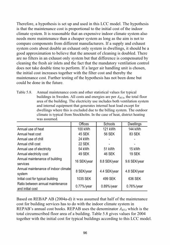
Therefore, a hypothesis is set up and used in this LCC model. The hypothesis is that the maintenance cost is proportional to the initial cost of the indoor climate system. It is reasonable that an expensive indoor climate system also needs more maintenance than a cheaper system as long as the aim is not to compare components from different manufacturers. If a supply and exhaust system costs about double an exhaust only system in dwellings, it should be a good approximation to believe that the amount of cleaning is doubled. There are no filters in an exhaust only system but that difference is compensated by cleaning the fresh air inlets and the fact that the mandatory ventilation control does not take double time to perform. If a larger air handling unit is chosen, the initial cost increases together with the filter cost and thereby the maintenance cost. Further testing of the hypothesis has not been done but could be done in the future.

Table 5.8. Annual maintenance costs and other statistical values for typical buildings in Sweden. All costs and energies are per ABTA, the total floor area of the building. The electricity use includes both ventilation system and internal equipment that generates internal heat load except for dwellings where this is excluded due to the billing system. The outdoor climate is typical from Stockholm. In the case of heat, district heating was assumed.

Offices Schools Dwellings

Annual use of heat 100 kWh 121 kWh 144 kWh

Annual heat cost 45 SEK 56 SEK 83 SEK

Annual use of chill 24 kWh - -

Annual chill cost 22 SEK - -

Annual use of electricity 54 kWh 51 kWh 15 kWh

Annual electricity cost 49 SEK 46 SEK 19 SEK

Annual maintenance of building

services16 SEK/year 8.8 SEK/year 9.6 SEK/year

Annual maintenance of indoor climate

system8 SEK/year 4.4 SEK/year 4.8 SEK/year

Initial cost for typical building 1035 SEK 499 SEK 636 SEK

Ratio between annual maintenance

and initial cost0.77%/year 0.89%/year 0.76%/year

Based on REBAP AB (2004a-d) it was assumed that half of the maintenance cost for building services has to do with the indoor climate system in REPAB’s annual cost books. REPAB uses the denominator ABTA which is the total circumscribed floor area of a building. Table 5.8 gives values for 2004 together with the initial cost for typical buildings according to this LCC model.

96

5.5.2 Repair

Costs for replacing components after their life time are called repair costs and are either planned or caused by a failure. The bathtub curve is sometimes used to describe the failure frequency with a lot of errors in the start of the life time due to initial problems and adjustment problems, fewer errors in the middle and more errors in the end of the life span due to the spread of the life time and the fact that components get worn out (Wilkins, 2002a; Wilkins, 2002b). A statistical approach could be chosen but would yield more input data.

Instead, repair costs are modelled as the cost to replace and by that renew components after their life time, which is the time they work. If the, user defined, life cycle is shorter than the life time of a component, no replacement occurs. The life time of components is discussed by Dahlblom (1999;2001). He indicates that the change of components usually occurs before they are actually worn out. The aim of this LCC model is not to model the behaviour of the building owner. Therefore, statistical data of how often components are actually changed must be combined with component life time data to avoid the risk that the building owner rebuilds the building after a shorter time. Rebuilding could be handled in this LCC model by inserting an appropriate life cycle and scrap value. This scrap value should describe the value of what can be kept of the indoor climate system at the rebuilding. The life cycle should end at the rebuilding time.

In this LCC model, it is proposed that components in the indoor climate systems that incorporate motors or electronics have a life time of 15 years and that other components have a life time of 40 years.

5.5.3 Space requirements

Typically, an indoor climate system takes up a different area and height depending on what system is used. If the site area is free, it can be argued that the building can be made a little larger to get the same useful floor area. With that approach, building costs are needed for more than the indoor climate system. To avoid this, the assumed approach for the LCC model is to let the LCC model user set a value per floor area that could have been used if the indoor climate system did not occupy it. Only areas that are influenced and different for different system are taken into account. Questioning of consultants has shown that the area that the indoor climate system occupies, and that affects the usable floor area, is the area for ventilation shafts and the area for the air handling unit room.

97

For the shafts in dwellings, the maximum branch duct diameter plus 200 mm is squared and summed as area per floor. These added 200 mm gives space for the insulation and mounting. For shafts in premises, it is assumed that the corridor or the room width is always enough to fit the main ducts. It is also assumed that the shaft length is constant for all storeys. Therefore the highest diameter of the main ducts times the highest of the room width and the corridor width is used as area for added space per floor.

Exhaust fans are usually mounted on the roof, which does not occupy any area. The air handling unit of detached houses is supposed to need the width of the unit times the depth times two. For larger air handling units, the needed area is assumed to be two times the length of the unit times the maximum of two times the width and the width plus 1.2 m. That is supposed to give enough space for the main silencers.

It can be argued that low speed diffusers need floor area close to the diffuser where the air speed exceeds 0.2 m/s. Since the solution with low speed diffusers is usually selected for other reasons, this is not taken into account. It can also be argued that a mixing system needs unnecessary floor height. This is not taken into account since buildings tend to have an unnecessary floor height for architectural reasons.

5.5.4 Performance and health

An interesting question regarding LCC for indoor climate systems is how the indoor air quality influences work productivity, health and comfort. To give an example of the influence, a typical office building with CAV ventilation is assumed to have an LCC over 40 years of 4000 SEK/m². If the airflow rate is doubled from the requirements in Sweden, also at nights, the LCC would increase by typically 1000 SEK/ m² based on the LCC model. Assume that there are 0.03 people/m², that a doubled airflow rate results in a productivity increase of 1.7% (Wargocki, 2000), that the salary cost is 150 SEK/h and that half of the entire working year is spent in the office, which means 850 hours. Over a 40 year life span with annually equal salary labour costs, the net present value can be found to be 28 times the single cost from Figure 4.1 with 2% discount interest rate.

These assumptions could result in a decreased life cycle cost for office labour of 0.03 · 0.017 · 150 · 850 · 28 SEK/m² = 1821 SEK/m². That means, if the benefit is true, with a clearly understated labour cost and a clearly overstated constant airflow rate approach, that it is a good investment from an LCC perspective to double the airflow rate. In this example, no health aspects were added.

98

There have been some recent studies regarding the issues of health and performance in indoor environment. Regarding health effects, the indoor air consists of several hundreds of chemicals (Fanger, 2005). Too little is known about many of these chemicals. Even less is known about their combined effects. Therefore, the understanding of the indoor environment influence on humans is far from finished. The studies done are either experimental, particularly regarding work performance, or epidemiological regarding health effects.

For example, the incidence of asthma and allergy has increased over time. So far, it is not well explained why. The indoor environment can be suspected to be a part of the explanation. Bornehag et al. (2004) performed a case-control study on children in 390 Swedish dwellings and found that the prevalence of allergic symptoms decreased significantly with an increased ventilation airflow rate. The dwellings were sorted into four quartiles depending on the airflow rate of 0.44 to 1.43 air changes per hour at a median of 0.62 as reference case. The odds ratio increased constantly to 1.95 for the group with 0.05 to 0.24 air changes per hour with a median at 0.17. The mean air change rate from the study was within the air change rate quartile with an odds ratio of 1.14 compared to the reference case. This quartile had a mean air change rate of 0.38. The reported prevalence of allergic symptoms was 9.7% based on a former cross-sectional study.

For a typical new detached house with typical data and 0.17 air changes per hour over 40 years, this LCC model gives an LCC of 1540 SEK/m² of which 570 SEK/m² is initial costs. If the air change rate is increased to 0.62, the LCC becomes 1790 SEK/m² of which 590 SEK/m² is initial costs. If the floor area is assumed to be 150 m², the increased airflow rate means an increased LCC of 60000 SEK. That increase could be compared with the cost and inconvenience related to allergy and asthma which was reported in around half of the cases of allergy (Bornehag et al., 2005a). Bornehag et al. (2005b) also showed, based on the same case-control study, a significantly increased prevalence of asthma and allergy at higher concentrations of certain kinds of phthalates in indoor dust. That concentration can be thought to depend on the ventilation airflow rate. The costs of health effects are not included in the LCC model.

Wargocki et al. (2005) showed a significantly increased performance from pupils in schools with higher airflow rates and not too high indoor temperatures based on an experimental study. The value of such a benefit is not calculated, but the study indicates the importance of a good indoor air quality and climate in schools.

99

Sick leave has been found to decrease with increasing ventilation airflow rate. Seppänen and Fisk (2005) presented a model for prevalence of short term sick leave based on Fisk et al. (2003) and Milton et al. (2000). Based on the prevalence of short term sick leave of 2% at 10.4 l/(s·person), Figure 5.15 gives the relative increase of productivity from decreased short term sick leave at different airflow rates where qref = 6.5 l/(s·person). For the purpose of the LCC model, a curve fit was made for these data according to Equation 5.45. It is reasonable to believe that the influence of the airflow rate is higher at low airflow rates. It is also reasonable to believe that the productivity reaches a maximum level at infinite airflow rate. Therefore, the exponential curve form is chosen.

1390.0

10189.0 refq

q

sl ePI (5.45)

Based on Heschong group (2003), Federspiel et al. (2004), Tham (2004), Tham and Willem (2004), Wargocki et al. (2004), Bako-Biro (2004), Wargocki et al. (2000) and Myhrvold and Olesen (1997), Seppänen and Fisk (2005) weighted the influence on work productivity from the airflow rate based on qref = 6.5 l/s according to Figure 5.15. The curve fit for the relative increase in work productivity on the same form as Equation 5.45 is given by Equation 5.46.

1478.0

10375.0 refq

q

wp ePI (5.46)

The combined effect of less short term sick leave and higher work productivity of the present people is calculated and shown in Figure 5.15. A curve fit for the combination is given by Equation 5.47. This equation can be used together with a salary cost in the LCC model to include the influence of higher airflow rate. The constants in the equation can be varied as well as qref to allow for future results in this research. The benefit is scaled by the occupancy rate and calculated hour for hour since the influence is not linear.

100

1444.0

10571.0 refq

q

q ePI (5.47)

Relative increase

-0.03

0

0.03

0.06

-1 0 1 2 3 4 5 6 7 8 9

q/qref -1

Added effects -

Seppänen and Fisk

Added effects -

Equation 5.47

Productivity -

Seppänen and Fisk

Productivity -

Equation 5.46

Sick leave decrease -

Seppänen and Fisk

Sick leave decrease -

Equation 5.45

Figure 5.15. The relative increase in productivity from a certain airflow rate with qref = 6.5 l/(s·person) based on Seppänen and Fisk (2005). The total productivity increase consists of both increased work productivity for the present people and a relative increase of the present people due to less prevalence of short term sick leave. The Equations given are curve fits used in the LCC model.

Seppänen and Fisk (2005) also looked at productivity related to temperature. Based on a weighting of 26 studies, they present a relative decrease in work performance according to Figure 5.16. In the LCC model, this decrease is modelled by a two degree polynomial curve fit according to Equation 5.48. It is a coarse assumption with the aim to decrease the need for input data. This polynomial approach is also used by Jönsson (2005). The reference temperature, tref, is 21.6°C according to Seppänen and Fisk (2005).

200155.0 refroomt ttPD (5.48)

101

Relative loss

0

0.05

0.1

0.15

0.2

15 20 25 30 35

Indoor temperature/°C

Seppänen

and Fisk,

2005

Equation

5.48

Figure 5.16. The relative decrease in productivity from a certain indoor temperature based on Seppänen and Fisk (2005). The Equation given is a curve fit used in the LCC model.

The LCC model includes the described equations to take into account the airflow rate and indoor temperature. The, by more and more research, indicated benefits from a better indoor climate would have a great impact on the LCC of an indoor climate system. Still, more research in this field is needed. There are still many questions and uncertainties regarding long term effects and combined effects. In this LCC model, it has been important to let the user decide such influences.

5.5.5 Scrap value

The scrap value is often set to zero if the life cycle is as long as a reasonable life time for a building (Flanagan et al., 1989). If the life cycle is many years and the discount interest rate is positive, the net present value of the scrap value is small and probably therefore often excluded. It is difficult to know what kinds of taxes and fees there will be 40 years ahead for disposals.

The user of the LCC model can set a scrap value. A scrap value can be used to model rebuilding. If the building will alter its function after five years, the calculation span can be set to five years and a scrap value can be inserted to take into account the costs for rebuilding the indoor climate system.

5.6 Aspects on algorithms and PC program

The LCC technique and a way to calculate initial costs as well as running costs has been presented. To apply this LCC model into a PC program, there must

102

be an order of calculations and decisions to end up with the LCC. The following steps are used in the PC program.

1. Collect input data about the economics, the building and the system, that should be analyzed. Collect input data on the outdoor climate for the normal year on the actual location.

2. Set all duct piece lengths according to the building geometry and the chosen system.

3. Set the occupancy levels of all four modelled zones to 100%. The cooling design is supposed to handle full occupancy.

4. Perform an annual energy use calculation for each zone on hourly basis. Let this calculation decide the zone airflow rate for every hour if it is a temperature controlled VAV ventilation system. If not, find the highest value of the power for support cooling. This value is meant to be the design value.

5. Split the zone flow rate between the rooms in each zone. 6. Sum the airflow rates for each storey, if exhaust air devices are used only

in the corridors.7. For each room, decide the size of each diffuser to handle the maximum

design airflow rate.8. For the hour with highest total airflow rate, calculate the maximum

pressure drop in the duct systems with the air terminals. This pressure drop is the design pressure drop. In a VAV ventilation system without main pressure feed back, this design pressure drop is supposed to be maintained constantly by the air handling unit. If several zones with different cooling needs are included in the calculation, there is a risk that the total maximum airflow rate does not correspond with the total maximum pressure drop. The approach is used anyway to avoid a pressure drop calculation for each annual hour. In the case of a CAV ventilation system with timer, the main pressure is decreased during nights. In that case, the maximum pressure drop for the low-airflow rate is needed. This must be calculated which yields two pressure calculations.

9. Calculate the annual energy needed to exchange the ventilation air and heat or cool the supply air on an hourly basis. Find the maximum power during the year for air cooling.

10. Set the occupancy levels to zero. The heating design is supposed to handle an empty building.

11. Perform an annual energy use calculation for each zone on an hourly basis. Find the maximum power needed for heating.

12. Set the sizes of other components than the duct system components and air terminals with regards to the dimensioning values.

103

13. Reset the occupancy levels to the estimated levels for the zones respectively.

14. Calculate the annual energy use on an hourly basis for each zone. 15. Sum the airflow rates for every hour for the zones and calculate the needed

energy to exchange the air and heat or cool the supply air. The pressure drop must be calculated for every hour if a VAV system with constant branch pressure and main pressure feed back is used.

16. Sum the costs for the components associated with and necessary for the chosen system.

17. Calculate energy, maintenance, space, repair and other costs. 18. Use the LCC technique on the calculated initial and future costs to obtain

the LCC.

5.6.1 Algorithmic aspects

The needed algorithms are all without internal iterations for solving implicit equations. In the steps given above, it is assumed that the maximum power design is based on the resulting extreme values based on the normal year. It could be possible to read outdoor climate data for extreme years for the maximum power design. For the maximum power design, the entire year is calculated. It would be possible to decrease the number of calculations if only the periods with the extreme outdoor climate data were used. In the case of CAV ventilation system without support cooling, there is no need to run the cooling power design part.

To be able to compare different systems, several calculations are needed. There has been no attempt to make algorithms to save calculations for series of analyses. The nature of the problem seems too complex. Optimisation of parameters such as size of the air handling unit or pressure drop per meter duct also requires several calculations.

5.6.2 PC program aspects

The given steps have been implemented into a computer program. In fact, the PC program development and the LCC model development have been parallel processes. Model aspects need to be tested and the simplest way to do so is often by the use of a computer program.

The PC program is made in the programming language Delphi, mainly in version 7 (Borland, 2005). Delphi is a Windows based programming language for event driven stand-alone applications to run under Microsoft Windows 32-bit operating systems. The code language is Object Pascal. The compiler is known to create fast running binary code. The choice of Delphi is mainly based on personal experience from the language and the fact that it creates fast

104

running Windows based applications that are stand-alone, which means that they do not need another program.

An alternative could have been Excel which many people are familiar with. Excel is thought to be too slow. It would also be difficult to make a good user interface. Javascript or another web-based language is an interesting alternative since the application would run from a web page. The updates would be easier and it would be platform independent. With the chosen approach, it would be too slow.

Even if there are many calculations to perform due to the hourly approach, a typical calculation takes about a second on a modern PC. More time is needed if the system is a VAV system with constant branch pressure and main pressure feedback because a pressure drop calculation is needed for every hour. No effort has been put on optimising the programming code.

So far the PC program calculates LCC for the indoor climate systems described in this section. The program has an input section for the geometrical building layout that corresponds to the LCC model given in this thesis. There is not yet an implementation of sensitivity analyses or other optimisation analyses. Still the program user can do a sensitivity analyses and optimisation by running the program several times with different input data. The program now consists of around 6000 code lines or 150 000 characters of code. Figure 5.1 shows the Swedish interface of the PC program at the present state.

One of the main problems encountered during the programming have been all the possible alternatives for the indoor climate system and its components. There has been a need for a lot of logic code to differ systems. Hopefully this, in parts, detailed LCC model can be a base for future simplifications. Another question is how the cost updates should be made. In the present version, new costs have to be inserted in the programming code. In the future, this could be part of a database solution.

5.6.3 Sensitivity analysis

Sensitivity analysis is necessary in these types of calculations since there are a lot of very unreliable input data. It is made by conscious changes in parameters affecting the calculation, one at a time or several. Typical parameters to change could be interest rates, occupancy levels or life spans.

105

A form of sensitivity analysis is to implement the Monte Carlo method (Flanagan et al., 1989). The user of the model has to give distribution data for each desired input parameter. Then, a desired number of calculations are made with randomly set input data according to the given distribution. This results in a certain output distribution.

106

6. Model results The LCC model is not yet comprehensively compared with other models and programs but some comparisons between the LCC model and the programs ENORM (Svensk Byggtjänst, 2000) and ISOVER ENERGI (ISOVER, 2005) regarding the energy use is performed. A simulation of a simple fictitious detached house located in Malmö with Atrans = 400 m² and ABTA = 200 m² with CAV supply and exhaust ventilation and leakage according to Boverket (2002) without windows resulted in a 0.6% higher heat use for ENORM and 5.3% higher heat use for ISOVER ENERGI. ENORM uses daily outdoor climate data from Malmö. For the ISOVER ENERGI program, outdoor climate data from Lund is the closest available, which is a slightly colder climate explaining the higher heat use. This default case has a 100 W internal heat load. If the internal heat load is increased to 1100 W, ENORM gives 0.2% higher value and ISOVER ENERGI gives 7.8% higher value. If, compared to the default case, 10 m² of windows are added in the south direction, ENORM gives a heat use 11% lower than the heat use from the LCC model. This indicates that ksolar could be increased. On the other hand, ENORM is known to over-estimate the benefit from solar radiation (Svensk Byggtjänst, 2000; Nilsson, 2003a). If an exhaust ventilation system is used compared to the default case, ENORM gives a value that is 5.5% higher than the LCC model. This can be explained by the over-estimated leakage in combination with exhaust ventilation systems in ENORM (Svensk Byggtjänst, 2000).

Based on the LCC model presented, some examples of life cycle cost analyses are given. The PC program implementation is used in its present state, still with a risk for bugs. Some parametric studies are performed to show the influence from some changes based on a default case for each example. In all examples, the LCC is given in SEK per ABTA excluding VAT. All cooling energy costs are declared as electricity costs.

6.1 One corridor office building

This example is an assumed one-corridor four storey cell office building with the corridor in the south-north direction. On each storey, there are 20 office cells. There are supposed to be 1 m² of windows in each room. The assumed data for the example is given in Table 6.1. The outdoor climate data are from Stockholm, Sweden.

The default indoor climate system is a supply and exhaust system with constant airflow rate, passive beams for support cooling and hydronic radiators for support heating. The air is supplied by ceiling diffusers and extracted from

107

each cell. The duct sizes are allowed to vary within the branches and main duct respectively. With this the set up, one zone is used. It is assumed that the office is designed for one person in each cell. Daytime is supposed to be between 08 and 18 five days a week. In the default case, no other costs are included. In the case of a VAV ventilation system, the supply air temperature is 16°C to increase the cooling power of the supply air and lower the LCC.

Table 6.1. Assumed data for the office building example.

BHF 3 m heat 90%

BLR 3 m COPchill 2

BLT 30 m troom min 21°C; max 24°C

BWC 3 m Pint occupied 25 W/m²

BWR 3 m Pint vacant 2 W/m²

ABTA 1080 m² OC daytime 50%

Atrans 19 m²/room OC other time 5%

Utrans 0.5 W/(m²·K) qvent 0.35 l/(s·m²)+7 l/person

R 1 Pa/m ccap·mcap/Acap 100000 J/(m²·K)

tsa 18°C ksolar 0.5

hr 80% kleak 0.8 l/(s·m²)

The price of heat is set to 0.6 SEK/kWh and the price of electricity is set to 0.8 SEK/kWh excluding VAT. The discount interest rate is assumed to be 1% for electricity, 2% for heat and 3% for other costs, representing a real price increase on heat and even more on electricity. An annual value of 1000 SEK/m² is assumed for space loss. It is assumed that there is a 20% deduction for the initial costs for both the air and hydronic components. The scrap value is assumed to be zero.

Over a 40 year period, the LCC is estimated to be 4562 SEK/m² referring to the area ABTA. Figure 6.1 shows the LCC subdivided into different parts. Figure 6.2 subdivides the initial cost. From the result it can be seen that only the airflow adjustment and silencers seems to be small enough to be possible to exclude.

108

Heat; 1330

Repair; 472

Space loss;

411

Maintenan-

ce; 340

Initial cost;

1558

Electricity;

451

Figure 6.1. The different components of the LCC in SEK/m² excluding VAT for the example in Section 6.1. The area in the denominator is ABTA

Silencers; 10

Air terminals;

72

Radiator

panels; 101

Passive

beams; 223

Heat pipes;

198

Control; 88

Air flow

adjustment;

10

Air handling

unit; 143

Heat plant; 38

Fire dampers;

64 Chill pipes;

230

Chill plant;

233

Exhaust duct;

66Supply duct;

81

Figure 6.2. The initial cost from Figure 6.1 subdivided in SEK/m² excluding VAT.

109

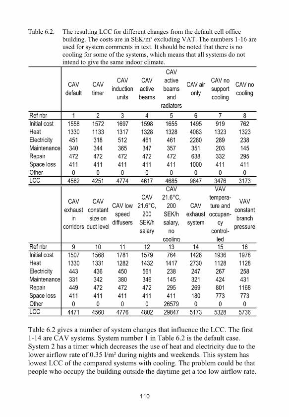
Table 6.2. The resulting LCC for different changes from the default cell office building. The costs are in SEK/m² excluding VAT. The numbers 1-16 are used for system comments in text. It should be noted that there is no cooling for some of the systems, which means that all systems do not intend to give the same indoor climate.

CAV

default

CAV

timer

CAV

induction

units

CAV

active

beams

CAV

active

beams

and

radiators

CAV air

only

CAV no

support

cooling

CAV no

cooling

Ref nbr 1 2 3 4 5 6 7 8

Initial cost 1558 1572 1697 1598 1655 1495 919 762

Heat 1330 1133 1317 1328 1328 4083 1323 1323

Electricity 451 318 512 461 461 2280 289 238

Maintenance 340 344 365 347 357 351 203 145

Repair 472 472 472 472 472 638 332 295

Space loss 411 411 411 411 411 1000 411 411

Other 0 0 0 0 0 0 0 0

LCC 4562 4251 4774 4617 4685 9847 3476 3173

CAV

exhaust

in

corridors

CAV

constant

size on

duct level

CAV low

speed

diffusers

CAV

21.6°C,

200

SEK/h

salary

CAV

21.6°C,

200

SEK/h

salary,

no

cooling

CAV

exhaust

system

VAV

tempera-

ture and

occupan-

cy

control-

led

VAV

constant

branch

pressure

Ref nbr 9 10 11 12 13 14 15 16

Initial cost 1507 1568 1781 1579 764 1426 1936 1978

Heat 1330 1331 1282 1432 1417 2730 1128 1128

Electricity 443 436 450 561 238 247 267 258

Maintenance 331 342 380 346 145 321 424 431

Repair 449 472 472 472 295 269 801 1168

Space loss 411 411 411 411 411 180 773 773

Other 0 0 0 0 26579 0 0 0

LCC 4471 4560 4776 4802 29847 5173 5328 5736

Table 6.2 gives a number of system changes that influence the LCC. The first 1-14 are CAV systems. System number 1 in Table 6.2 is the default case. System 2 has a timer which decreases the use of heat and electricity due to the lower airflow rate of 0.35 l/m² during nights and weekends. This system has lowest LCC of the compared systems with cooling. The problem could be that people who occupy the building outside the daytime get a too low airflow rate.

110

Induction units and active beams are both expensive products according to systems 3 and 4. In system 4, the active beam is supposed to fulfil the support heating. It can be questioned if such a system works. In system 5, hydronic radiators are used together with the active beam which results in a slightly higher LCC.

If the airflow rate is set to handle the cooling in the worst situation, as in system 6, the ventilation system becomes more expensive but there is no need for hydronic cooling and passive beams. The need for heat and electricity and in turn the LCC becomes very high. This is not a reasonable system. Perhaps this system could benefit slightly from a lower supply air temperature.

If there is no support cooling, but still chilled supply air, see system 7, the need for cooling electricity decreases. The need for heat decreases slightly due to the thermal capacity in combination with excessive temperatures in the room during parts of the year. No cooling at all as in system 8 decreases initial and running costs further and in turn the LCC. In system 12, the indoor temperature has been kept at 21.6°C constantly compared to system 1. Loss due to decreased work performance has been added according to Equation 5.46 in the field ‘Other’. This means that there will be no other costs. If the cooling is removed from that system, see system 13, the building will have high temperatures during part of the year. The initial cost decreases but the LCC increases a lot due to productivity losses. The aspect of window airing has not been taken into account. This aspect would influence the real situation and dampen the benefit of cooling because people air the room when it is too hot.

If the exhaust air is taken from the corridors on each storey, the initial cost decreases. The fan electricity for the exhaust fan also decreases. This is exemplified in system 9. In system 10, there is constant duct sizes for each entire branch and a constant duct size in the main duct. This decreases the LCC slightly. Low speed diffusers are more expensive resulting in a higher LCC according to system 11. The use of heat decreases due to the higher exhaust temperatures. System 14 shows an exhaust system. The use of heat increases due to the lack of heat recovery.

System 15 is a VAV system controlled by occupancy and temperature. The use of heat and electricity decreases. However, the LCC still increases due to the increased initial cost for the more expensive components and their maintenance. System 16 has an even higher LCC even though the electricity use is lowered, due to the lower main pressure after the air handling unit during parts of the year.

111

LCC/(SEK/m²)

0

2000

4000

6000

8000

10000

12000

0 50 100 150 200

Life span/years

VAV

CAV

Figure 6.3. The LCC as a function of calculation life span for the two systems 1 and 15 in Table 6.2.

LCC/(SEK/m²) - CAV

0

1000

2000

3000

4000

5000

6000

14 16 18 20 22

tsa/°C

VAV

14 16 18 20 22

tsa/°C

Space loss

Repair

Maintenance

Electricity

Heat

Initial

Figure 6.4. The LCC as a function of the supply air temperature for the systems 1 and 15 in Table 6.2.

Figures 6.3-6.11 show the LCC for system 1 in the case of CAV and system 15 in the case of VAV in Table 6.2. Figure 6.3 shows the LCC as function of time. Figure 6.4 shows the influence of the supply air temperature. A high supply air temperature in the VAV system needs high airflow rates. Figure 6.5 shows the influence from maximum pressure drop per meter duct. The influence is small. At the life span of 40 years, the optimal pressure drop seems to be higher than accepted for noise generation reasons. For R = 5.06 Pa/m, the LCC is increasing again for the VAV system.

112

LCC/(SEK/m²) - CAV

0

1000

2000

3000

4000

5000

6000

0.44 0.67 1 1.5 2.25 3.38

R/(Pa/m)

VAV

0.44 0.67 1 1.5 2.25 3.38

R/(Pa/m)

Space loss

Repair

Maintenance

Electricity

Heat

Initial

Figure 6.5. The LCC as a function of the maximum pressure loss per meter duct for the systems 1 and 15 in Table 6.2.

LCC/(SEK/m²)

0

3000

6000

9000

-4 -2 0 2 4

Inflation rate difference/%

Space loss

Repair

Maintenance

Electricity

Heat

Initial

Figure 6.6. The LCC as a function of the inflation as a difference compared to the default case.

Figure 6.6 shows the influence from different discount interest rates. The inflation rate difference has been subtracted from the discount interest rates for electricity, heat and others respectively. Figure 6.7 shows the LCC for different average U-values of the building envelope. Less insulation means higher need for heating and higher designed power for heating resulting in more expensive components. The electricity for cooling decreases since most of the hours in Stockholm are colder outdoors than indoors. Figure 6.8 gives

113

the energy use of the LCC as a function of the thermal mass of the interior. It is shown that there is a decrease in both heating and cooling.

LCC/(SEK/m²)

0

2500

5000

7500

10000

0 0.13 0.25 0.5 1 2

Uav /(W/(m²·K))

Space loss

Repair

Maintenance

Electricity

Heat

Initial

Figure 6.7. The LCC as a function of the average U-value of the envelope for the default CAV system.

LCC energy/(SEK/m²)

1300

1400

1500

1600

1700

1800

1 10 100 1000

(ccap·mcap/Acap)/(kJ/(m²·K))

Electricity

Heat

Figure 6.8. The energy part of the LCC as a function of the average thermal mass of the interior for the default CAV system.

114

LCC/(SEK/m²) - CAV

0

1000

2000

3000

4000

5000

6000

0 20 40 60 80 100

hr/%

VAV

0 20 40 60 80 100

hr/%

Space loss

Repair

Maintenance

Electricity

Heat

Initial

Figure 6.9. The LCC as a function of the temperature efficiency of the heat recovery for the systems 1 and 15 in Table 6.2.

.

LCC/(SEK/m²) - CAV

0

1000

2000

3000

4000

5000

6000

0 25 50 75 100

Daytime occupancy rate/%

VAV

0 25 50 75 100

Daytime occupancy rate/%

Space loss

Repair

Maintenance

Electricity

Heat

Initial

Figure 6.10. The LCC as a function of the daytime occupancy rate for the systems 1 and 15 in Table 6.2.

Figure 6.9 evaluates the benefit from the heat recovery. In the LCC model, there are no corrections for pressure drop due to the temperature efficiency. There is also no cost influence due to the temperature efficiency. Figure 6.10 indicates an optimal daytime occupancy rate. Occupancy heats the building by internal heat gains but a too high occupancy results in heat gains that must be cooled. The LCC does not include electricity associated with heat loads. Figure 6.11 gives the LCC for different locations. In Madrid the normal annual average outdoor temperature is 14.8°C, in Stockholm it is 6.7°C and in Karasjok it is -2.5°C. The higher need for heating in Karasjok is obvious. The

115

higher need for cooling in Madrid certainly needs a larger system in the VAV case with rather high design airflow rates.

LCC/(SEK/m²) - CAV

01000200030004000500060007000

Madrid

Sto

ckholm

Kara

sjo

k

Location

VAV

Madrid

Sto

ckholm

Kara

sjo

k

Location

Space loss

Repair

Maintenance

Electricity

Heat

Initial

Figure 6.11. The LCC for three different locations for the systems 1 and 15 in Table 6.2.

LCC/(SEK/m²)

0

10000

20000

30000

40000

6.5 10 20 40 60 80

qv ent/(l/(person·s))

Other

Space loss

Repair

Maintenance

Electricity

Heat

Initial

Figure 6.12. The LCC as a function of the airflow rate per person if work productivity as a function of the airflow rate is taken into account in the category ‘Other’. This work productivity cost is adjusted absolutely to be zero at 80 l/(person·s) and to be seen as a cost at lower airflow rates.

Figure 6.12 shows the LCC of the CAV default system as a function of the airflow rate per person if a salary cost is assumed to be 200 SEK/hour excluding VAT, and the influence from better work productivity is taken into

116

account according to Equation 5.46. An optimum is found far above the airflow rates that are commonly used in buildings.

Cost/(SEK/m²) - CAV

0

4000

8000

12000

0 25 50 75 100

Number of rooms per storey

VAV

0 25 50 75 100

Number of rooms per storey

LCC 1

LCC 4

LCC 10

In.1

In.4

In.10

Figure 6.13. The LCC for the systems 1 and 15 in Table 6.2 when the number of rooms per storey and the number of storeys are varied with the rest of the data as default. The numbers in the legend refer to the number of storeys. ‘In.’ refers to the initial cost.

Figure 6.13 gives the influence from the size of the building. For the VAV system, there is an optimum where the LCC per total floor area is minimal. For the CAV system, there is no optimum. The PC program only handles 100 rooms per storey in its present state. In the LCC model, it is assumed there is always space enough in the false ceiling. This is probably not the case with so many rooms. It is not reasonable to have that many rooms on one branch with the typical layouts assumed in the LCC model.

6.2 School

This example is assumed to be a two-storey, single sided school with the corridor in the south-north direction. On each storey, there are 6 classrooms. There are supposed to be 10 m² of windows facing west. The assumed data for the building is given by Table 6.3. The outdoor climate data are from Stockholm, Sweden.

The default indoor climate system is a supply and exhaust system with constant airflow rate and hydronic radiators for support heating. The air is supplied by ceiling diffusers and extracted from each classroom. There is no cooling. The duct sizes are allowed to vary within the branches and main duct respectively. With this the set up, one zone is used for the energy and power use calculation. In each classroom, there is assumed to be a maximum of 30

117

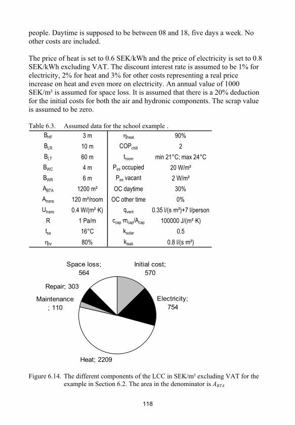
people. Daytime is supposed to be between 08 and 18, five days a week. No other costs are included.

The price of heat is set to 0.6 SEK/kWh and the price of electricity is set to 0.8 SEK/kWh excluding VAT. The discount interest rate is assumed to be 1% for electricity, 2% for heat and 3% for other costs representing a real price increase on heat and even more on electricity. An annual value of 1000 SEK/m² is assumed for space loss. It is assumed that there is a 20% deduction for the initial costs for both the air and hydronic components. The scrap value is assumed to be zero.

Table 6.3. Assumed data for the school example .

BHF 3 m heat 90%

BLR 10 m COPchill 2

BLT 60 m troom min 21°C; max 24°C

BWC 4 m Pint occupied 20 W/m²

BWR 6 m Pint vacant 2 W/m²

ABTA 1200 m² OC daytime 30%

Atrans 120 m²/room OC other time 0%

Utrans 0.4 W/(m²·K) qvent 0.35 l/(s·m²)+7 l/person

R 1 Pa/m ccap·mcap/Acap 100000 J/(m²·K)

tsa 16°C ksolar 0.5

hr 80% kleak 0.8 l/(s·m²)

Initial cost;

570

Electricity;

754

Heat; 2209

Maintenance

; 110

Repair; 303

Space loss;

564

Figure 6.14. The different components of the LCC in SEK/m² excluding VAT for the example in Section 6.2. The area in the denominator is ABTA

118

Over 40 year period, the LCC is estimated to 4510 SEK/m² referring to the area ABTA. Figure 6.14 gives the LCC subdivided into different parts. Figure 6.15 subdivides the initial cost. From the result it can be seen that some categories are zero since there is no cooling in the default case.

Silencers; 10

Air terminals;

28

Radiator

panels; 55

Passive

beams; 0Heat pipes;

112

Air handling

unit; 152

Heat plant; 37

Control; 0

Air flow

adjustment; 2

Supply duct;

75

Exhaust duct;

62

Chill plant; 0

Chill pipes; 0

Fire dampers;

37

Figure 6.15. The initial cost from Figure 6.14 subdivided in SEK/m² excluding VAT.

Table 6.4. The resulting LCC for some alternatives for the example based on the default school building. The costs are in SEK/m² excluding VAT. The numbers 1-6 are used for system comments in text.

CAV default CAV timer

CAV timer,

low speed

diffusers

CAV timer,

cooling

VAV

occupancy

controlled

VAV temp.

and oc.

controlled

Ref nbr 1 2 3 4 5 6

Initial cost 570 569 600 1403 691 1291

Heat 2209 1028 1021 1058 765 773

Electricity 754 272 273 525 136 362

Maintenance 110 110 115 354 132 322

Repair 303 303 303 361 375 602

Space loss 564 564 564 564 564 900

LCC 4510 2847 2875 4266 2663 4250

Table 6.4 gives the LCC for some alternative systems based on the default case. With the low occupancy rate that can be suspected in schools, a timer is

119

beneficial, as shown in system 2. Low speed diffusers, in system 3, do not make the LCC much higher. System 5 uses occupancy controlled variable airflow rate resulting in the lowest LCC. If cooling is desired, the VAV system 6 is still preferable for the CAV system 4. Cooling increases the costs of an indoor climate system remarkably.

Figure 6.16 shows the influence from varying occupancy rates at daytime for the CAV system with timer and the VAV system controlled by occupancy. At high daytime occupancy rates, the benefit from the variable airflow rate does not compensate for the higher initial cost.

LCC/(SEK/m²)

0

1000

2000

3000

4000

0 25 50 75 100

Daytime occupancy rate/%

VAV

CAV

Figure 6.16. The LCC for system 2 and 5 in Table 6.4 as a function of the daytime occupancy rate.

6.3 Apartment building

An apartment building is assumed to have four storeys with two one-room, two two-room, two three-room and two four-room apartments on each storey. Assumed data for the building is given by Table 6.5. The outdoor climate data are from Stockholm, Sweden.

The default indoor climate system is an exhaust system with constant airflow rate and hydronic radiators for support heating. There is no cooling. The duct sizes are allowed to vary within the branches and main duct respectively. With this the set up, four zones are used for the energy and power use calculation.

120

Table 6.6 gives the apartment areas, the window areas, the heat transmission areas and the number of people per apartment. Daytime is supposed to be between 08 and 18 five days a week. No other costs are included.

Table 6.5. Assumed data for the example apartment building.

BHF 3 m COPchill 2

BLT 43.3 m troom 22°C

BWT 12 m Pint occupied 3 W/m²

ABTA 2080 m² Pint vacant 2 W/m²

COPHP 3 OC daytime 30%

Utrans 0.365 W/(m²·K) OC other time 70%

R 1 Pa/m qvent 0.35 l/(s·m²)

tsa 18°C ccap·mcap/Acap 100000 J/(m²·K)

hr 80% ksolar 0.4

heat 90% kleak 0.8 l/(s·m²)

Table 6.6. Assumed areas and number of people for the example apartment building. 1 room 2 rooms 3 rooms 4 rooms

Number of

persons/apartment1 2 3 4

Window area 3 m² 6 m² 8 m² 9 m²

Apartment area 30 m² 50 m² 80 m² 100 m²

A trans /apartment 34.2 m² 57 m² 91.2 m² 114 m²

The price of heat is set to 0.6 SEK/kWh and the price of electricity is set to 0.8 SEK/kWh excluding VAT. The discount interest rate is assumed to be 1% for electricity, 2% for heat and 3% for other costs representing a real price increase on heat and even more on electricity. An annual value of 800 SEK/m² is assumed for space loss. It is assumed that there is a 20% deduction from the initial costs for both air and hydronic components. The scrap value is assumed to be zero.

Over a 40 year period, the LCC is estimated to be 1871 SEK/m². Figure 6.17 gives the LCC subdivided into different parts. Figure 6.18 subdivides the initial cost. The exhaust system used as default has no cost for the supply duct system.

121

Initial cost;

437

Electricity;

47

Heat; 1155

Maintenance

; 97

Repair; 27

Space loss;

108

Figure 6.17. The different components of the LCC in SEK/m² excluding VAT for the example in Section 6.3. The area in the denominator is ABTA

Silencers; 14

Air terminals;

88

Radiator

panels; 110

Heat pipes;

131

Air flow

adjustment; 3

Heat plant; 30Air handling

unit; 17Exhaust duct;

44

Supply duct; 0

Figure 6.18. The initial cost from Figure 6.17 subdivided in SEK/m² excluding VAT.

Table 6.7 gives the LCC for some alternative systems based on the default case. The air is supplied by ceiling diffusers for systems 2 and 4. The systems with heat recovery, either supply and exhaust system with heat recovery unit or exhaust system with exhaust air heat pump, have lower LCCs. The gained heat from the exhaust air heat pump is assumed to 60% of the available. This gain is 62 kWh/m². It should be reasonable to supply that amount of recovered

122

heat into hot tap water and hydronic heating. The annual need for hydronic heating without heat recovery is 70 kWh/m². If cooling is added, see system 4, the LCC increases mostly regarding initial, maintenance and repair costs. Figure 6.19 shows the LCC for the system 2 and 3 in Table 6.7. In this figure, it is assumed that the heat gain from the exhaust air heat pump never exceeds 62 kWh/m². Therefore, system 2 recovers more of the heat at high airflow rates.

Table 6.7. The resulting LCC for some alternatives for the example based on the default apartment building. All systems are CAV systems. The costs are in SEK/m² excluding VAT. The numbers 1-4 are used for system comments in text.

ExhaustSupply and

exhaust

Exhaust with

exhaust air

heat pump

Supply and

exhaust,

cooling

Ref nbr 1 2 3 4

Initial cost 437 523 476 916

Heat 1155 546 140 582

Electricity 47 182 593 428

Maintenance 97 112 105 225

Repair 27 79 91 170

Space loss 108 278 108 278

LCC 1871 1721 1513 2600

LCC/(SEK/m²) - SEH

0

1000

2000

3000

4000

0.2 0.35 0.5 1

qv ent/(l/(s·m²))

EHP

0.2 0.35 0.5 1

qv ent/(l/(s·m²))

Space loss

Repair

Maintenance

Electricity

Heat

Initial

Figure 6.19. The LCC for system 2 and 3 in Table 6.7 as a function of the airflow rate per floor area. SHE means supply and exhaust and EHP, exhaust with exhaust air heat pump.

123

6.4 Detached house

A detached house is assumed with two storeys with nrsupply = 5. The assumed data for the building is given in Table 6.8. The outdoor climate data are from Stockholm, Sweden. The default indoor climate system is an exhaust system with constant airflow rate and hydronic radiators for support heating. There is no cooling. The duct sizes are allowed to vary within the branches and main duct respectively. Four persons are assumed to live in the house.

Table 6.8. Assumed data for the example detached building.

BHF 3 m COPchill 2

BLT 12 m troom 22°C

BWT 8 m Pint occupied 3 W/m²

ABTA 192 m² Pint vacant 1 W/m²

Atrans 288 m² COPHP 3

Awindow 15 m² OC daytime 30%

Utrans 0.25 W/(m²·K) OC other time 70%

R 1 Pa/m qvent 0.35 l/(s·m²)

tsa 18°C ccap·mcap/Acap 0

hr 80% ksolar 0.5

heat 90% kleak 0.8 l/(s·m²)

Daytime is supposed to be between 08 and 18 five days a week. No other costs are included. The prices of heat is set to 0.6 SEK/kWh and the price of electricity is set to 0.8 SEK/kWh excluding VAT. The discount interest rate is assumed to be 1% for electricity, 2% for heat and 3% for other costs representing a real price increase on heat and even more on electricity. An annual value of 400 SEK/m² is assumed for space loss. No deduction from the initial costs is assumed. The scrap value is assumed to be zero.

124

Initial cost;

526

Electricity;

84

Heat; 1139

Repair; 29Space loss;

12

Maintenance

; 129

Figure 6.20. The different components of the LCC in SEK/m² excluding VAT for the example in Section 6.4. The area in the denominator is ABTA

Silencers; 18

Air terminals;

33

Radiator

panels; 89

Heat pipes;

178

Supply duct; 0Exhaust duct;

31

Air handling

unit; 18

Heat plant;

158

Air flow

adjustment; 1

Figure 6.21. The initial cost from Figure 6.20 subdivided in SEK/m² excluding VAT.

125

Table 6.9. The resulting LCC for some alternatives for the example based on the default detached house. All systems are CAV systems. The costs are in SEK/m² excluding VAT. The numbers 1-6 are used for system comments in text

ExhaustSupply and

exhaust

Exhaust air

heat pump,

45% gain

Exhaust air

heat pump,

60% gain

Exhaust air

heat pump,

75% gain

Supply and

exhaust,

cooling

Ref nbr 1 2 3 4 5 6

Initial cost 526 587 579 579 579 1546

Heat 1139 702 539 339 139 704

Electricity 84 149 419 526 632 322

Maintenance 129 138 138 138 138 458

Repair 29 108 114 114 114 170

Space loss 13 42 13 13 13 42

LCC 1920 1726 1802 1709 1616 3241

The LCC for a 40 year life cycle is estimated to be 1920 SEK/m² referring to the area ABTA. Figure 6.20 shows the LCC subdivided into different parts. Figure 6.21 subdivides the initial cost. The exhaust system used as default has no cost for the supply duct system. The heat pipes make up a remarkable part of the initial cost as well as the heat plant. The heat plant cost is used from the LCC model but should be analyzed further.

Table 6.9 gives the LCC for some alternative systems based on the default case. The air is supplied by ceiling diffusers for systems 2 and 6. There is a benefit from heat recovery. Depending on the possible gain from the exhaust air heat pump, the system with lowest LCC is either system 2, 4 or 5. Cooling is also expensive here but should be much less expensive with other equipment in a real case, for example an air to air heat pump or air conditioner. Figure 6.22 shows the LCC for system 2 in Table 6.9 as a function of the airflow rate. The LCC is not increasing proportionally to the airflow rate.

126

LCC/(SEK/m²)

0

500

1000

1500

2000

2500

0 0.2 0.35 0.5 1

qv ent/(l/(s·m²))

Space loss

Repair

Maintenance

Electricity

Heat

Initial

Figure 6.22. The LCC for system 2 in Table 6.9 as a function of the airflow rate per floor area.

127

128

7. Discussion and conclusions An LCC model for indoor climate systems is presented. This LCC model is implemented into a PC program that has been tested on some examples of buildings. The LCC model takes into account the indoor climate system based on single components with data from the manufacturer. The needed components are determined from typical building layouts. The energy use is calculated and put together with estimated maintenance, repair and space loss costs. This gives the LCC.

The LCC model is still not thoroughly tested and compared to other programs. In the future, comparisons with other programs should be made, for example based on standard test houses. Within the European Commission, a number of standards are being developed to support the EU Directive on the Energy Performance of Buildings. These standards should be compared to the LCC model to allow the LCC model to be adjusted and refined.

This LCC model is rather limited regarding indoor climate systems and even more regarding buildings. In a building design process, this LCC model needs to be combined with other decision criteria regarding the indoor climate system as well as life cycle cost aspects regarding the entire building. For example, life cycle assessment and the resulting indoor environment including lighting and sound are of interest. Today, there is a need for a number of tools to perform all needed analysis if a number of decision criteria will be used. In the future, perhaps these tools could be combined into a single building design program.

7.1 Applicability of the LCC model and PC program

To end up with a PC program that will be used in the building industry, the need for input data should not be too high. Hopefully, the need for input data to the proposed LCC model is not more than reasonable to obtain in the early stage of the building design process. In the building industry, the PC program, and not the LCC model, is the obvious way to reach the users. The PC program implementation should be possible to use almost as is by building designer, but there is a need for some further testing and user interface refinements.

Although primarily Swedish conditions are modelled, the LCC model should be applicable to other locations although the costs are for typical components bought in Sweden. Outdoor climate from all over the temperate world is included in the PC program. If the components are bought in Sweden or

129

bought for Swedish costs, and the system is included in the LCC model, it should be possible to use it internationally but it is up to the user of the LCC model to assure that the input data are reliable and with appropriate validity. The typical return air system of the US is not modelled but may be approximated with the right approach regarding the outer fan efficiencies and an adjusted relative humidity in the outdoor climate.

In the future, the applicability of the LCC model and the PC program will hopefully be tested in the building industry. This should provide answers to questions regarding refinements of the user interface of the PC program. The cost and data update for the LCC model and the computer program based on the LCC model is an issue that needs to be solved to be able to use the tool in the future. At this point, data must be updated manually by recoding and recompiling the program. The cost data of Wikells byggberäkningar AB (2003) is updated every second year so that is not an impossible task. If the PC program should handle data for many countries, there must be a user interface for inserting and updating costs. It would be interesting for the future to make connections between costs databases and this tool to get a self updating tool.

The LCC model can also be used for addressing development questions regarding indoor climate systems. It can help to tell where to put the effort to, for example, obtain better and more energy efficient indoor climate systems for the future. The flexibility of the LCC model also enables testing of system combinations that are not used or not available on the market.

7.2 Model results

The results from the calculated examples give an idea of the most important parameters. It should be pointed out that the electricity used for the equipment that generates the internal heat gain is not included in the electricity cost. A higher internal heat load will decrease the need for heating. If such costs would be included in the LCC as electricity cost, the LCC would benefit from lower internal heat loads.

7.2.1 Initial versus running costs

There seems to be an existing myth in the building industry that the running costs make up 95% of the LCC. In all the examples, the initial cost is a much larger part of the LCC, particularly for cell offices, where it can be 35% for a 40 year life span. If the life span is shorter, the initial cost makes up a larger part of the LCC. Perhaps, the myth originates from analyses of single components. For a fan or a pump it could be true that 95% of the LCC is running costs. The fan cost divided by the total energy cost is 1.5% for the

130

detached house example. As a comparison, the ratio between the initial cost and the LCC is 83% for a theoretical duct according to Paper V.

Heating energy is a large part of the LCC for all examples. This is explained by the rather cold climate in Stockholm and the fact that the buildings in the examples are not used during nights. Cooling makes up a remarkable part of the initial cost, at least if hydronic systems, that are modelled here, are used. The pipe system is expensive and the chilling plant that is included is expensive. The energy cost for cooling is lower. For the examples, cooling is included in the electricity cost. For the default office building example, cooling makes up 198 SEK/m² while heating makes up 1330 SEK/m² despite the lower discount interest rate for electricity than for heat. The office building example with outdoor climate data for Madrid shows a higher cooling cost than heating cost.

7.2.2 CAV versus VAV

The office building example has a CAV system as default. For the VAV system, there is much more initial cost due to the diffusers and the control system. This indicates that development resources should be spent on lowering the costs for electronics and ‘active’ components if the aim is to sell energy efficient and flexible indoor climate systems. It can also be believed that the costs for electronic components have decreased since the year of 2003 which the costs in the LCC model refer to.

A timer added to the CAV system decreases the LCC due to lower airflow rates during nights. In the examples, a rather high airflow rate was set during nights. It should be reasonable to save even more energy by a lower airflow rate during nights. Regarding CAV system with timer, it can be argued that different systems are not compared in a fair way since a VAV system would provide a visitor in a cell during nights with the required amount of airflow rate while the CAV system with timer will not.

For the school building, the timer added to the CAV system is even more beneficial due to the high airflow rate per floor area in that example. Here, each component needed for a VAV system handles a higher airflow rate, which makes this system profitable. Also with cooling, the VAV system has lower LCC than the CAV system. If the occupancy rate during daytime is high, the timer in the CAV system does almost the same work as the VAV system. If the occupancy rate during daytime is low, the VAV system enables a more occupancy corrected airflow rate, resulting in a lower LCC.

131

7.2.3 Exhaust versus supply and exhaust ventilation

For dwellings, it is shown that heat recovery is a good solution from the LCC perspective as well as from the energy perspective. The exhaust air heat pump gives the lowest LCC for both the apartment building example and the detached house example. The unintentional leakage decreases with the exhaust system and the recovered heat can be used all the year. A risk is that the heat pump needs more maintenance than modelled. Another problem is that the supplied air is cold during the winter time and that the supply airflow rate is not very precisely distributed between the rooms in the dwelling. For example, an opened window in the kitchen can zero the supply airflow rate in the bedroom. Therefore it can be questioned if the exhaust system should be compared with a supply and exhaust system.

Another question about the exhaust air heat pump is the ratio between the electricity and heat price. If that ratio exceeds the coefficient of performance of the exhaust air heat pump, COPHP, the heat pump is not of use. As shown, the heat recovery unit in a supply and exhaust system needs a much higher ratio to be useless.

7.2.4 Indoor climate system parameters

A number of parametric variations are presented in the examples. Pressure drop per meter duct has low influence. Supply air temperature has slightly higher influence. The temperature efficiency of the heat recovery unit has high influence. It is not modelled how the temperature efficiency influences the costs and outer fan efficiencies of the air handling unit but the saved heating should have the outstanding influence.

In the examples, different system changes are tested. Regarding the office building, there is a high influence from cost of components that are needed in every cell. Typically, this is the case with VAV controllers, or supply diffusers. The use of main pressure feedback in a VAV system needs some expensive components but decreases the fan electricity use. Exhaust air in the corridors on each storey decreases the initial cost as well as the fan energy cost slightly. It also gives air changes in the corridors and seems to be a recommendable solution.

The LCC for dwellings as a function of the airflow rate is presented. The LCC is almost a linear function to the airflow rate with an added constant at a zero airflow rate. If a higher airflow rate is shown to be needed in the future, for example for health reasons, there is a risk that the recovered heat from the exhaust air heat pump can not be utilized which is beneficial for the supply and exhaust system with heat recovery.

132

7.2.5 Building parameters

The average U-value of the building envelope and the location of the building has a large impact on, in particular, the heating use in Swedish climates. This implies that a building designer should carefully take into account the building envelope at the building design. The building location could be difficult to alter. The thermal mass has a small influence.

7.2.6 Human dependent parameters

Daytime occupancy rate does not influence the LCC much. The heat gain is replaced by cooling need at high occupancy rates. The discount interest rate is also shown to have a high influence, at least if the life span is not very short.

An included increase in work productivity is shown to have the highest influence on the LCC for indoor climate systems. There is most likely a lot still to discover in the area of performance, health and comfort effects from the indoor climate. The solution is not only to increase the airflow rate. Probably, a combination of pollution control and ventilation control is needed. The future will hopefully tell what kind of indoor climate systems and indoor materials should be used. It seems to be naive to exclude the effects on the human from the indoor climate. The human dependent parameter is an important part of a sensitivity analysis.

7.3 Simplifications

Still, there are a lot of simplifications and assumptions made within the LCC model. Based on the influence from the pressure drop per meter duct and the occupancy rates, the simplifications based on the appended Paper IV and V seems to be appropriate. There are a lot of more determining parameters that are uncertain. Still, it is thought to be a strength to model the duct system in a detailed way and to differ daytime occupancy from the occupancy for the rest of the time. It is reasonable to find input data for these two occupancy rates although it is not reasonable to find data on which part of the building that is occupied at a certain time at the early stage of the building design process.

For dwellings, exhaust ventilation is a common alternative. For the choice between exhaust system and supply and exhaust system, the unintentional leakage has an important influence. The results from the appended Paper VII are used to model this difference depending on the choice of system.

Outdoor climate data are taken from simulated data. The appended Paper VI shows an error for the degree hours regarding the time of the day. This error seems to be positive before noon and negative compared to the average error

133

after noon. That means that the high error part occurs both during night and daytime. The low error part also occurs both during night and daytime. Therefore, this error is believed to have a small effect on the result in combination with the fact that occupancy data can be rather uncertain.

There are simplifications and assumptions made for the energy calculations. A number of parameters are assumed to be constant to avoid iterative calculations and to simplify the calculations. Regarding the exhaust airflow rate for systems with heat recovery unit, the airflow rate is influenced by the air density downstream from the heat recovery unit. For the larger air handling units included in the LCC model, this is compensated for by the air handling unit control. Therefore, there should be no correction for the air density in the calculations. For the smaller air handling units, it introduces an error. At low temperatures, the density influence will increase the under-pressure indoors that, in fact, will lower the leakage loss, which decreases the error in the calculations.

7.4 LCC model and PC program refinements

The LCC model and the PC program need some refinements to make the program useful. For example, help texts are needed as well as features to save data and present results graphically. Automatic parametric studies and an automatic calculation of all possible systems would also help the user but is not implemented yet. It should also be an option to insert parts of results from other sources and programs.

Other refinements could be made to increase the flexibility of the LCC model and program. Hydronic pipe systems are modelled with an assumed size instead of a calculated, power dependent size. This could be refined in the future. The method of handling thermal mass in combination with power design assumes that the requirements on the indoor temperatures are always fulfilled. This condition could be too extreme if the indoor temperature should go from a lower value at night to a higher value at daytime immediately. This could also be refined in the future. The requirements are supposed to be valid for all hours of the year. Still, the user of the LCC model can set and change the requirements to see the effect of different requirements. The user of the LCC model can also insert a real or fictitious outdoor climate and test the sensitivity for different outdoor climates. A cost that depends on the average U-value of the building envelope or the window area could be added to the LCC model to give the opportunity to optimise insulation thickness or window area.

134

So far, cooling recovery is not modelled. The use of it can decrease the energy use for cooling and the needed power for cooling but not much in a Swedish outdoor climate. It could be a feature in the future. The heat recovery is modelled with constant temperature efficiency. At a lower airflow rate than the nominal, the temperature efficiency increases. That can also be realised in the future. In the case of support cooling, there is no control regarding condensation. The condensation in the chilling coil could be examined further in the future. The constant approach for the coefficient of performance of cooling plants is a simplification that decreases the need for input data regarding the plant and temperature levels. The constant approach regarding coefficient of performance of an exhaust air heat pump should be good since the conditions of such a heat pump are rather constant.

7.5 Future research

During this project, a number of aspects on the indoor climate system and its LCC have been excluded due to the scope of the project. Deeper knowledge in the areas of these aspects could help to refine the LCC model and deepen the understanding of indoor climate systems. This could help to solve the main question of how we should maintain a good indoor climate.

The maintenance costs are modelled in a simple way. These costs could be analyzed further based both on theoretical work and empirical studies. It would also be of interest to analyse the influence that the initial cost has on the maintenance costs. This influence could be based on different components, experiences or theories. Is an expensive air handling unit better than a cheap one from an LCC perspective?

Rebuilding could be studied both in regards to the influence on the LCC due to different rebuilding actions and the human behaviour regarding rebuilding. Particularly for premises, it can be believed that rebuilding and changing the building activity happens rather often and has a rather high impact on the LCC of the indoor climate system as well as on the entire building LCC.

The LCC model shows that the initial cost of components have a high influence on which system has the lowest LCC, at least if the work performance is not included. Is it best to spend the money on a consultant with good negotiation skills or an LCC analysis of the indoor climate system? Work is desired regarding verification of initial cost data on components. In this LCC model, the listed costs are used without further investigation of deductions, geographical influence or others. The problem with such work could be the increasing influence of the global market.

135

An interesting question is how the market value of the house is influenced by the choice of indoor climate system and its running costs. This could be studied and put in the perspective of the energy declarations needed as a result of the Energy Performance of Buildings directive from the European Commission.

On a more technical level, there is need for more analyses regarding the air handling unit and its efficiency. This LCC model has a coarse approach that probably should be refined to handle each size of air handling units separately. The air handling units should be ‘opened up’ and analysed regarding their internal design and its influence on the LCC of the indoor climate system. Is the air handling unit optimized as a unit? Another technical question to ask is if the indoor climate system components can be designed to give more efficient ventilation or better indoor climate.

The energy supply system should be studied in combination with the indoor climate system and the building. For example, it would be interesting to examine the influence on the coefficient of performance regarding different ways to cool a building or the influence of the boiler efficiency regarding different ways to heat a building. The possible and available supply systems are probably very different for different buildings and locations.

Other aspects on the indoor environment, such as noise and light, are of interest to analyse from an LCC perspective. Work that puts together the indoor climate system with other parts of a building to obtain an optimised building could be the final aspiration.

136

8. References Al-Hammad, A.M., Fahd, K. (1992), An overview of life cycle cost models used in the assessment of building insulation materials, Housing Science,16, (2), pp123-136

Anger, Y., Ohlsson, H. (2004), Sänkta boendekostnader genom energieffektivisering, Building Services, Lund University, Lund, Sweden, Report TVIT—04/5002, in Swedish

Arditi, D.A. (1996), Life-cycle costing in municipal construction projects, Journal of Infrastrucutre Systems, 2 (1), pp5-14

ASHRAE (2003), ASHRAE Handbook—HVAC Applications, Atlanta: American Society of Heating, Refrigerating and Air-Conditioning Engineers, United States

ASHRAE (2004), ASHRAE Handbook—HVAC Systems and Equipment,Atlanta: American Society of Heating, Refrigerating and Air-Conditioning Engineers, United States

Bako-Biro, Z. (2004), Human perception, SBS symptoms and performance of office work during exposure to air polluted by building materials and personal computers, Doctoral thesis, International Centre for Indoor Environment and Energy, Technical University of Denmark

Beacom, V.A. (1984), Life-cycle costing for HVAC, and more, Specifyingengineer, 51 (1), pp68-71

Bergsten, B. (2004), Free Cooling in Commercial Buildings – Application with Evaporative Cooling Tower and Chilled Beams, Building Services Engineering, Chalmers University of Technology, Gothenburg, Sweden, D 2004:05

Borg, M. (2001), Environmental Assessment of Materials, Components and Buildings – Building Specific Considerations, Open-loop Recycling, Variations in Assessment Results and the Usage Phase of Buildings, Building material, KTH, Stockholm, Sweden, Doctoral thesis, 2001:4

Borland (2005), Delphi 2005, Programming language developer http://www.borland.se/delphi/index.html, 2005-09-15

137

Bornehag, C.G., Sundell, J., Weschler, C.J., Sigsgaard, T., Lundgren, B., Hasselgren, M., Hägerhed-Engman, L. (2004), The Association between Asthma and Allergic Symptoms in Children and Phthalates in House Dust: A Nested Case-Control Study, Environmental Health Perspective, 112 (14), pp1393-1397

Bornehag, C.G., Sundell, J., Hägerhed-Engman, L. Sigsgaard (2005a), Association between ventilation rates in 390 Swedish homes and allergic symptoms in children, Indoor Air, 15, pp275-280

Bornehag, C.G., Sundell, J., Hägerhed-Engman, L. Sigsgaard, T., Janson, S., Aberg, N., DBH Study group (2005b), ‘Dampness’ at home and its association with airway, nose, and skin symptoms among 10851 preschool children in Sweden: a cross-sectional study, Indoor Air, 15, pp48-55

Boverket (2002), Boverkets byggregler – BFS 1993:57 med ändringar till och med 2002:19, Karlskrona, Sweden, in Swedish

Bull, J.W. (1993), Life Cycle Costing for Construction, London: Blackie Academic & Professional, United Kingdom

Cao, M., Cao, J. (2005), Optimal design of thermal-energy stores for boiler plants, Applied Energy, 83, pp55-68

Christianson, L.L., Fehr, R.L. (1983), Ventilation – Energy and Economics, ASAE Monograph, 6, pp333-349

Concannon, P. (2002), Residential Ventilation, AIVC Technical Note, 57, Brussels, Belgium, http://www.aivc.org, 2005-09-01

Dahlblom, M. (1999), Installationer ur ett livscykelperspektiv – En litteraturstudie, Dep. of Building Services, Lund University, Sweden, Report TABK—99/3058, in Swedish

Dahlblom, M. (2001), Orsaker till byte av VVS-installationer –En intervjuundersökning, Dep. of Building Services, Lund University, Sweden, Report TABK—01/1020. in Swedish

Day, A.R, Knight, I., Dunn, G., Gaddas, R. (2003), Improved methods for evaluating base temperature for use in building energy performance lines, Building Services Engineering Research & Technology, 24 (4), pp221-228

138

Durairaj, S.K., Ong, S.K., Nee, A.Y.C., Tan, R.B.H. (2002), Evaluation of Life Cycle Cost Analysis Methodologies, Corporate Environmental Strategy, 9 (1)

Enberg, H. (1995), Minimikrav på luftväxling, Enköping, Sweden, in Swedish

Engdahl, F. (2002), Air - for Health and Comfort – An anlysis of HVAC Systems’ Performance in Theory and Practice, Doctoral thesis, Dep. of Building Physics, Lund University, Sweden, Report TVBH-1013

Equa (2005), IDA Indoor climate and energy 3.0, Computer program, http://www.equa.se/, 2005-06-01

Euroace (2005), Energy Performance in Buildings Directive,http://europa.eu.int/comm/energy/demand/legislation/buildings_en.htm, 2005-08-30

Eurovent (2001), Life Cycle Cost, Review, ed. Becirspahic, S., May 2001, s.becirspahic@eurovent-certification.com

Fanger, P.O. (2005), What is IAQ?, Proceedings of the 10th International Conference on Indoor Air Quality and Climate, Beijing, China, P-1

Federspiel, C.C., Fisk, W.J., Price, P.N., Liu, G, Faulkner, D, Dibartolemeo, D.L., Sullivan, D.P., Lahiff, M. (2004), Worker performance and ventilation in a call center: analyses of work performance data for registered nurses, IndoorAir, 14 (8), pp41-50

Fisk, W.J., Seppänen, O., Faulkner, D. Huang, J. (2003), Economizer system cost effectivness: accounting for the influence of ventilation rate on sick leave, Proceedings of ISIAQ 7th International Conference Healthy Buildings 2003,Singapore, 3, pp361-367

Flanagan, R., Norman, G., Meadows, J., Robinson, G. (1989), Life Cycle Costing – Theory and Practice, BSP Professional Books, Oxford, United Kingdom

Florides, G.A., Tassou, S.A., Kalogirou, S.A., Wrobel, L.C. (2002), Measures used to lower building energy consumption and their cost effectiveness, Applied Energy, 73, pp299-328

139

Goodfellow. H., Tähti, E., editors (2001), Industrial Ventilation – Design Guidebook, Academic press, London, United Kingdom

Gustafsson, S.I., Karlsson, B.G. (1988), Why is life-cycle costing important when retrofitting buildings, International Journal of Energy Research,12 (2), pp233-242

Gustafsson, S.I., Karlsson, B.G. (1989), Life-cycle cost minimization considering retrofits in multi-family residences, Energy and Buildings,14 (1), pp9-17

Hasan, A. (1999), Optimizing insulation thickness for buildings using life cycle cost, Applied Energy, 63, pp115-124

Heikkilä, K. (2003), Environmental Assessment of Air-conditioning Systems in Offices – Some Aspects Related to System Design, Building Services Engineering, Chalmers University of Technology, Gothenburg, Sweden, D 2003:05

Hens, H.L.S.C., Mohamed, F.A., Verbeeck, G. (2002), Using Energy Life Cycle Costs as an Instrument for Optimisation, Proceedings of the Sustainable Building Conference in Oslo, 400

Heschong Mahone group (2003), Windows and offices: A study of office workers performance and the indoor environment, Prepared for California energy commission, Fair Oaks, California

Hodowanec, M.M. (1999), Evaluation of Antifriction Bearing Lubrication Methods on Motor Life-Cycle Cost, IEEE Transactions on Industry Applications, 35 (6)

ISOVER (2005), ISOVER ENERGI, Computer program for building energy use calculations, http://www.isover.se, 2005-09-01

IVT (2005), Discussion with the manufacturer, http://www.ivt.se/, 2005-06-01

Jagemar, L. (1991), Energiekonomi – Val av fläktar och kanalutformning för luftbehandlingssystem i servicelokaler och industrier, Building services engineering, Chalmers, Gothenburg, Sweden, D10:1991, in Swedish

James, N., Phillips, P.E. (1992), Spreadsheet application for HVAC operation cost comparisons, Energy Engineering, 89 (1)

140

Jensen, L. (1986), Energibesparingsekonomi, Building services, Lund University, Sweden, Report BKL1986:24, in Swedish

Jensen L. (1995), Beräkningsuttryck för PFS, Building Services, Lund University, Lund, Sweden, Report TABK—95/7022, in Swedish

Jensen, L. (2000), Injustering av ventilationssystem – underlag för implementering, Building Services, Lund University, Lund, Sweden, Report TABK—00/7058, in Swedish

Jenssen, B. (2003), Natural ventilation in Buildings – Detailed prediction of Energy Performance, Department of Energy and Process Engineering, NTNU, Trondheim, Norway, Doctoral thesis 2003:72

Johansson, P., Svensson, A. (1998), Metoder för mätning av luftflöden i ventilationsinstallationer, Byggforskningsrådet, Stockholm, Sweden, T22:1998

Johnson, E. (2001), Projekteringsmetodik för minimering av miljöpåverkan, Building Services Engineering, Chalmers University of Technology, Gothenburg, Sweden

Jorgensen, M, (2000), Faldgruber i investeringsanalyser, Dansk VVS/VVB,3-2000, Denmark, in Danish

Jönsson, A. (2005), Indoor temperature as a goods and as a factor of production, Proceedings of the 10th International Conference on Indoor Air Quality and Climate, Beijing, China, 1-3.01

Jönsson, Å. (1998), Life Cycle Assessment of Building Products – Case Studies and Methodology, School of Environmental Sciences, Technical Environmental Planning, Chalmers University of Technology, Gothenburg, Sweden, Doctoral thesis

Karyagina, M., Wong, W., Vlacic, L. (1998), Life cycle cost modelling using marked point processes, Reliability Engineering and System Safety,59, pp291-298

141

Kleiven, T. (2003), Natural ventilation in Buildings – Architectural concepts, consequences and possibilities, Department of Architectural Design, History and Technology, Norwegian University of Science and Technology, Trondheim, Norway, Doctoral thesis 2003:13

Källblad, K. (1998), Thermal Models of Buildings, Determination of Temperatures, Heating and Cooling Loads. Theories, Models and Computer Programs, Building Science, Lund University, Lund, Sweden, Doctoral thesis TABK--1015

LB-Hus (2005), Manufacturer of pre-fabricated detached houses, http://www.lbhus.se/, 2005-05-31

Leech, J.A., Wilby, K., McMullen, E., Laporte, K. (1996), The Canadian human activity pattern survey: Report of Methods and Population Surveyed, Chronic Diseases in Canada, 17, 3/4

Lewald, A., Karlsson, B.G. (1988), Evalutation model for optimal LCC in existing electric heated houses, International council for building research studies and documentation CIB report 107, pp175-183.

Lutz, J., Lekov, A., Chan, P., Dunham-Whitehad, C., Meyers, S., McMahon, J. (2005), Life-cycle cost analysis of energy efficiency design options for residential furnaces and boilers, Energy, 31, pp311-329

Malinowski, J. (2004), Energy-efficient Motors and Drives, AHRAE Journal,46 (1), pp30-32

Meteotest (2003), Meteonorm handbook, manual and theoretical background,Switzerland, http://www.meteonorm.com/, 2005-06-01

Milton, D.K., Glencross, P.M., Walters, M.D. (2000), Risk of sick leave associated woth outdoor air supply rate, humidification and occupant complaints, Indoor Air, 10, pp212-221

Myhrvold, A., Olesen, E. (1997), Pupils health and performance due to renovation of schools, Proceedings of Healthy Buildings/IAQ 1997, 1, pp81-86

Nelson, C.R., Schwert, G.W. (1977), Short-term interest rates as predictors of inflation: On testing the hypothesis that the real rate of interest is constant, The American Economic Review, 67, pp478-486

142

Nibe (2005), Discussion with the manufacturer, http://www.nibe.se/, 2005-06-01

Nilsson, A. (2003a), Energianvändning i nybyggda flerbostadshus på Bo01-området i Malmö, Building Physics, Lund University, Lund, Sweden, TVBH-3045, in Swedish

Nilsson, L.J. (1995), Air-handling energy efficiency and design practices, Energy and Buildings, 22, pp1-13

Nilsson, P.E. (1994), Heating and Cooling Requirements in Commercial Buildings – A Duration Curve Model including Building Dynamics, Building Services Engineering, Chalmers University of Technology, Gothenburg, Sweden, Doctoral thesis, D27:1994

Nilsson, P. E., editor (2003b), Achieving the desired indoor climate,Studentlitteratur, Lund, Sweden

PM-Luft (2005), PM Win software, http://www.swegon.se, 2005-05-31, Computer program

Pyrko, J., Norén, C. (1998), Effekthushållning i byggnader – Kunskapsläge och forskningsfront 1998, Dep. of Heat and Power Engineering, Lund University, Sweden, Report: TMVK—3183—SE, in Swedish

REPAB AB (2004a), Underhållskostnader, Mölndal, Sweden, in Swedish, ISSN 1404-6377, http://www.repab.se, 2005-09-14

REPAB AB (2004b), Årskostnader – Bostäder, Mölndal, Sweden, in Swedish, ISSN 1404-6377, http://www.repab.se, 2005-09-14

REPAB AB (2004c), Årskostnader – Kontor, Mölndal, Sweden, in Swedish, ISSN 1404-6377, http://www.repab.se, 2005-09-14

REPAB AB (2004d), Årskostnader – Skolor, Mölndal, Sweden, in Swedish, ISSN 1404-6377, http://www.repab.se, 2005-09-14

Riedel, T., Tiemann, N., Wahl, M.G., Ambler, T. (1998), LCCA – Life cycle cost analysis, IEEE AUTOTESTCON Proceedings – IEEE Systems Readiness Technology Conference, pp43-47

143

Ruegg, R.T., Petersen, S.R. (1985), New software aids life cycle costing of energy conservation projects, Heating-Piping-Air-Conditioning,57 (9), pp79-87

SCB (2003), Energy statistics for one- and two-dwelling buildings in 2002,Statistiska meddelanden, EN 16 SM 0302, Sweden, http://www.scb.se/Statistik/EN/EN0102/2003M00/EN16SM0302.pdf,2005-02-03

SCB (2004), Energistatistik för småhus, flerbostadshus och lokaler 2003,Statistiska meddelanden, EN 16 SM 0404, http://www.scb.se/, 2005-05-31, in Swedish

SCB (2005), Consumer price index 1830-2004, Statistiska meddelanden, PR 15 SM 0501, http://www.scb.se/, 2005-05-31, in Swedish

Schulz, L. (2003), Normalårskorrigering av energianvändningen i byggnader – en jämförelse av två metoder, EFFEKTIV, Sweden, 2003:01, ISBN 91-7848-932-6, http://www.effektiv.org/pdf_filer/Rapport%202003-01.pdf, 2005-09-22

Sellers, D.A. (2005), Rightsizing air handlers for lowest life-cycle cost, HPACHeating, Piping, AirConditioning Engineering, 77 (2), pp26-34

Seppänen, O., Fisk, W.J. (2005), Some quantitative relations between indoor environmental quality and work performance and health, Proceedings of the 10th International Conference on Indoor Air Quality and Climate, Beijing, China, P-4

Statens Energimyndighet (2005), Energiläget i siffror 2004, Eskilstuna, Sweden, http://www.stem.se/, 2005-06-01

Sterner, E. (2000), Life cycle costing and its use in the Swedish building sector, Building research and information, 28, pp368-375

Strusoft (2003), VIP+, software manual, Limhamn, Sweden, http://www.strusoft.com (2005-02-04), in Swedish

Ståhl, L., Wallace, M. (1995), Life Cycle Cost Comparison – Traditional Cooling Systems vs. Natural Convection Based Systems, TelecommunicationsEnergy Conference, 1995. INTELEC '95., 17th International, pp259-265

144

Sundell, J., Kjellman, M. (1994), Luften vi andas inomhus, Folhälsoinstitutet 1994:16, Stockholm, Sweden, in Swedish

Svensk Byggtjänst (2000), Enorm 1000, Manual, http://www.byggtjanst.se/, in Swedish

Svensson, A. (2003), Bra ventilation, Svensk ventilation, http://www.svenskventilation.se/, 2005-05-31, in Swedish

Sveriges Verkstadsindustrier (2001), Kalkylera med LCC energi,Industrilitteratur, Stockholm, Sweden, in Swedish

Sveriges Verkstadsindustrier (1996), ENEU 94, Stockholm: Sveriges Verkstadsindustrier, Sweden, in Swedish

Swegon (2005), Interview with Torvald Gunnarsson, Swegon, Norrköping, Sweden

Tham, K.W. (2004), Effects of temperature and outdoor air supply rate on the performance of call center operators in the tropics, Indoor Air, 14, pp119-125

Tham, K.W., Willem, H.C. (2004), Effects of reported neurobehavioral symptoms on call center operator performance in the tropics, Proceedings of RoomVent 2004, Coimbra, Portugal

Tighe, S. (2001), Guidelines for probabilistic pavement life cycle cost analysis, Transportation Research Record, 1769, pp28-38

Torsell, R. (2005), Energianvändning och livscykelkostnad för ventilations- och uppvärmningssystem i småhus, Building Services, ReportTVIT—05/5004, Lund University, Lund, Sweden, in Swedish

Tozer, R., Valero, A., Lozano, M.A. (1999), Thermoeconomics applied to HVAC systems, ASHRAE Transactions, 105 (1), pp1247-1255

Trinius, W. (1999), Environmental Assessment in Building and Construction – Goal and Scope Definition as Key to Methodology choices, Building Materials, KTH, Stockholm, Sweden, Doctoral thesis, TRITA-BYMA 1999:9

UNFCCC (2005), United Nations Framework Convention on Climate Change,http://unfccc.int/, 2005-05-31

145

Vattenfall (1994), Lokalerna och energihushållningen, Vattenfall Support, Stockholm, Sweden, in Swedish

Vik, T. A. (2003), Life Cycle Cost Assessment of Natural Ventilation Systems,Norwegian University of Science and Technology, Trondheim, Norway, Doctoral thesis 2003:14

Warfvinge, C. (2003), Installationsteknik AK för V, Building services, Lund University, Lund, Sweden, Report TABK--94/7016

Wargocki, P., Wyon D.P., Sundell, J., Clausein, G., Fanger O. (2000), The effects of outdoor air supply rate in an office on perceived air quality, sick building syndrome (SBS) symptoms and productivity, Indoor Air,10, pp222-236

Wargocki, P., Wyon, D.P., Fanger, P.O. (2004), The performance and subjective responses of call-center operators with new and used supply filters at two supply air flow rates, Indoor Air, 14, pp7-16

Wargocki, P., Wyon, D., Matysiak, B., Irgens, S. (2005), The effects of classroom air temperature and outdoor air supply rate on the performance of school work by children, Proceedings of the 10th International Conference on Indoor Air Quality and Climate, Beijing, China, 1-3.13

Wen, J., Smith, T.F. (2001), Effect of Thermostat Time Constant on Temperature Control and Energy Consumption, SIcon’01 Sensors for Industry Conference, Rosemount, Illinois, US

Wheatley, G. (2002), Oversized and underachieving, World Pumps,430, pp38-41

Wikells Byggberäkningar AB (2003), Sektionsfakta-VVS, Wikells byggberäkningar AB, Växjö, Sweden, http://www.wikells.se/, 2005-05-31, in Swedish

Wikells Byggberäkningar AB (2004), Sektionsfakta-El, Wikells byggberäkningar AB, Växjö, Sweden, http://www.wikells.se/, 2005-05-31, in Swedish

Wikells Byggberäkningar AB (2005), Interview of Carl Ehrnfrid Olsson, Wikells byggberäkningar AB, Växjö, Sweden, http://www.wikells.se/, 2005-05-31, in Swedish

146

Wilkins, D.J. (2002a), The Bathtub Curve and Product Failure Behavior Part One – The Bathtub Curve, Infant Mortality and Burn-in, Reliability HowWire,21, http://www.weibull.com/hotwire/issue21/hottopics21.htm, 2005-09-20

Wilkins, D.J. (2002b), The Bathtub Curve and Product Failure Behavior Part Two - Normal Life and Wear-Out, Reliability HowWire, 22, http://www.weibull.com/hotwire/issue22/hottopics22.htm, 2005-09-20

Yang, H., Burnett, J., Lau, K., Lu, L. (2001), Comparing central and split air-conditioning systems, ASHRAE Journal, 43 (5), pp36-38

Zinn, L., Stigson, C. (1993), Mikroventilation – ett värmeväxlande rumsaggregat, Building Services, Lund University, Lund, Sweden, Report TABK—93/5004, in Swedish

Öfverholm, I. (1998), Livscykelkostnader i den tidiga projekteringsfasen – cybernetiska betraktelsesätt, Institutionen för Arkitektur och stadsbyggnad, KTH, Stockholm, Sweden, Doctoral thesis, TRITA-ARK 1998:2, in Swedish

147

148

149

150

A life cycle cost approach to optimising

indoor climate systems

PAPER I

Dennis Johansson, Anders Svensson (2003) In Construction Process Improvement,eds. Atkin, B., Borgbrant, J., Josephson, P.E., Blackwell Science, Oxford, Great Britain

151

152

A LIFE CYCLE COST APPROACH TO OPTIMISING INDOOR CLIMATE SYSTEMS

Dennis Johansson & Anders Svensson

Introduction

An indoor climate system must fulfil some important functions. It must meet its design criteria, which means correct temperatures and clean air as required. Additionally, the system must consume the least amount of resources as possible from both an economic and environmental perspective. As a general rule, the construction sector in Sweden consumes about 40%, or about 154 TWh, of the total energy used in the country (Energimyndigheten, 2000). A major part of this is used to provide buildings with the necessary energy for heating and cooling. Another factor is that the design of indoor climate systems has been overly focused on initial or capital costs and less on operating costs.

With a life cycle approach, both the environmental and economic performance of the indoor climate system could be improved. Today, there is a lack of knowledge and tools for determining life cycle costs. Research is therefore needed. This chapter discusses how to create a model for life cycle cost (LCC) analyses of different indoor climate solutions and discusses the need for such a model.

State-of-the-art review

In order to create the right indoor climate system, it is important to decide on what people demand from their indoor climate. Ideas for establishing methods and devising tools for LCC analyses are also important. Here, the ongoing research as well as the existing tools will be discussed. In order to optimise the costs from the client’s perspective, a life cycle approach is needed to deal with whole buildings or even several buildings and their locations, the tenants involved, social systems, migration and so on. To solve such a problem requires that life cycle analyses must be subdivided into smaller more manageable calculations. It is important to decrease the complexity, but still keep the bigpicture in view.

First, research dealing with ventilation is reviewed. Second, life cycle costs for the building, as well as indoor climate systems, are discussed. The last section deals with examples and the impact of ventilation on work performance and health.

153

Ventilation principles and functionality

The basic types of ventilation systems available today include natural ventilation, mechanical exhaust ventilation and mechanical supply-exhaust ventilation. The latter can incorporate a heat exchanger. Natural ventilation uses thermal driving forces and wind pressure. It works best in the wintertime, is very quiet and needs little maintenance. Problems with this system can include weather dependency and the difficulty of controlling ventilation rates. In some cases, it is impossible to achieve sufficient airflow rates. Natural ventilation is less common in today’s design, but mixed systems known as hybrid ventilation are increasing and a number of research projects are investigating their performance.

Mechanical exhaust ventilation draws air from outlet devices that are located in the kitchen and the bathroom where the air is most polluted. This creates a lower pressure inside the building, with supply air coming through inlet devices in the wall. A common problem is that an open window, for example in the kitchen, changes the pressure balance resulting in zero airflow in a bedroom when the bedroom door is closed (Engdahl, 1999). Exhaust ventilation can be fitted with a heat recovery unit, providing a positive influence on the system’s life cycle cost.

Supply and exhaust ventilation has two fans supporting both supply and exhaust air. Here, it is easy to add a heat exchanger for heat recovery from the outlet air. Normally, the exhaust airflow rate is slightly greater than the supply rate so that moisture is not driven through the walls. A problem is that the exhaust filter must be cleaned or replaced more often than the supply filter, because of the more polluted indoor air; if it is not, the exhaust airflow rate will decrease. Supply and exhaust air systems are a more expensive solution, but provide the best control over flow patterns and flow rates (Engdahl, 2000).

Functionality is an essential feature of an indoor climate system and the main reason for implementing it. In Sweden, as in other countries, there are recommendations and legal demands setting the airflow rates and temperatures in buildings. Mandatory Swedish ventilation control regulations reflect experiences from practice. They imply that research about the ventilation process must focus on questions regarding the human need for good indoor air quality as well as for a good indoor climate without noise and drafts. More than half of all schools, offices and multi-dwelling buildings failed their mandatory ventilation control test according to Engdahl (1998): mandatory ventilation controls started in 1992 and the client must attend to any faults. The worst cases were natural ventilation systems.

It is important that a ventilation system continues to operate for its design life. The system must be self-adjusting or the system must be adjusted whenever a change is made or age alters the performance of the system. Office buildings are prone to frequent refurbishment and hence a lot of money can be spent on altering the ventilation system. However, a flexible ventilation system can be

154

self-adjusting and can accommodate new demands brought about by refurbishment.

The literature abounds with papers on room air distribution, numerical methods and indoor air quality. For example, the energy efficiency of displacement and mixing ventilation has been compared in an environmental chamber study and displacement ventilation was shown to be the best (Awbi, 1998). Published studies can be helpful when deciding if a proposed ventilation system is likely to work properly in a given situation. If it is unlikely to work, there is no need to calculate the LCC.

A related project to the one discussed in this chapter is ongoing. This deals with determining optimal control strategies to achieve lower energy use and better functionality. For example, by controlling the flow rate and the supply air temperature for an exhaust and supply air system, the energy use and, thereby, the LCC can be decreased. Today, control strategies seem to be simplified as much as possible. One major result so far is that condensation occurring by air cooling is an important factor.

LCC principles, tools, use and research

Whole life cycle cost or simply life cycle cost (LCC) is the total cost a client pays for a product. The LCC consists of the investment cost, energy cost, maintenance cost, demolition cost and all other recurrent costs, which are normally discounted to today’s value, known as the present value, by the use of an estimated interest rate.

Difficulties with LCC analyses include uncertain input data that depend upon human actions within society as well as variability in technical performance. The lifetime of the product is not easy to decide upon and much depends on processes like changes in business activity and technical limitations. In terest rates are extremely difficult to predict with any certainty. Energy cost, outdoor climate and client behaviour are other uncertain aspects (Bull, 1993; Flanagan etal., 1989). How many different costs should be taken into account? For example, improved work performance due to better indoor air quality can be significant, but is seldom taken into account.

Life cycle thinking, based on experience as opposed to formalised techniques, is often used though not to its full potential. For example, disposable items are not used in a kitchen because they would be more expensive in the long run. A life cycle approach has also been used in other sectors like national defence, road construction and agriculture. Often, in the construction sector, some sort of life cycle perspective is taken, but this tends to rely on old experience (or even perceptions) of good solutions. This may not be the best solution. In the construction process, the constructor often pays for the investment cost, but does not guarantee long-term functionality. There are no incentives for the constructor to undertake LCC analyses, so long as clients do not require them.

155

To give an example, one survey has indicated that 40% of municipal construction projects in the US were based on LCC analyses. The reasons given for not using LCC analyses were lack of guidelines and the difficulty of estimating future costs (Arditi, 1996). A survey undertaken in 1999 shows that 66% of clients surveyed use life cycle cost analyses to some extent in building projects (Sterner, 2000). Life cycle cost analysis is rarely adopted in all phases of the construction process. Lack of tools and knowledge is cited as a significant reason.

Interest in making LCC analysis routine has resulted in many practical guidelines and forms. One such example is Energy Efficient Procurement, ENEU 94,(Sveriges verkstadsindustrier, 1996), which is a tool for determining the life cycle cost of a fan system. ENEU 94 was updated in 2001 and is available on the web only. The idea is to calculate the LCC for given scenarios and to compare them. ENEU is also a form of guidelines with the aim of forcing the design consultants to undertake the analysis in order to secure the contract. The guidelines have been developed mainly to help determine the optimal size of an air handling unit: special control strategies for air handling plant have not been included.

ENEU 94 does not incorporate spatial costs or system functions. If a number of competing consultants make one or even several calculations each, a good solution might be found, but it is not guaranteed. ENEU 94 takes much more than air handling into account, for example electrical motors and machines.

An EC-supported project is developing guidelines similar to ENEU 94 and carries the name, LCC-based Guidelines on Procurement of Energy Intensive Equipment in Industries (Eurovent, 2001). In ENEU 94, there is a client focus, but the EC project has a producer focus.

The Norwegian University of Science and Technology (Vik, 2001) has an ongoing project dealing with life cycle costs for natural ventilation systems. One aim of the project is to determine when natural and hybrid ventilation results in a low life cycle cost.

LCC analyses for indoor climate systems

LCC analyses are increasingly undertaken by researchers, consultants and clients to determine the best ventilation system. These analyses most often compare two or more types of systems, but they do not come up with a completely optimised solution. 85% of the energy used over the lifetime of a building is consumed during the occupation phase. The majority of this is due to the building’s heating and cooling systems (Adalberth, 2000). The energy used within an indoor ventilation system is the balance between energy saving and sufficient airflow rates for a clean indoor environment.

Office cooling can be achieved either by an all-air system or radiant cooling system. It is generally expected that a radiant cooling system uses less energy

156

than an air system because of decreased air movement. A saving potential of 10% was found in a Japanese study (Imanari et al., 1999). In another example, a chilled ceiling was used in an office building providing a slightly better indoor climate in addition to the energy saving. A German study (Sodec, 1999), found a lower LCC for radiant cooling ceilings, when compared with an all-air system, assuming the systems are well designed and operated correctly. In the US, 30% less energy use for a radiant system was found. The peak power use was also discussed. The decrease in peak power could reach 27% (Stetiu, 1999). The peak power cost can be taken into account in the LCC analysis. In the US, as in other hot countries, a lot of cooling is required compared to Sweden and northern Europe, where the power supply problems appear in the winter time. Then the heating peak power is of greater interest.

A deficiency in these studies was that the all-air system could be improved by better control strategies. Also, the features with increased airflow from the all-air system were not discussed; neither was heating discussed and this is an important part of energy use in northern Europe. There remains a need for a more systematic approach to designing complex indoor climate systems.

A comparison of radiant cooling and all-air cooling has been discussed in the context of a life cycle assessment approach (Johnsson, 2001). In a life cycle assessment, environmental impact determines the system instead of its costs. The environmental impact is obtained from the assumed danger of sub-activities. Johnsson tested two different methods to provide comparative results.

There was some work dealing with the optimisation of duct sizes (Besant et al.,2000; Jensen, 2000). Expressions were written to describe both the energy costs and the materials and installation costs, to yield an optimised pipe system. This is usable, but whole indoor climate systems or combinations of systems were not optimised.

A central cooling system was compared to a split system in a 29-storey office building in Hong Kong. The central system gave the lowest LCC (Yang et al.,2001). However, Yang et al. only discuss the comparison between two scenarios; there could be an even better system, so the general system approach is still missing.

Matsson (1999) has made some life cycle cost calculations for systems with different control strategies. Three systems were compared; one with a constant air volume flow (CAV), one with a variable air volume (VAV) with constant pressure in the main duct and one with a variable air volume with changeable pressure in the main duct in order to minimise the static pressure. The analyses were based on the real costs for a school and an office building. The system with changeable pressure in the main duct shows the lowest life cycle cost in both cases due to the lower pressure drop decreasing the energy used.

157

The heating or cooling system can also include the production of power. The heating system for housing was found to be of great importance when determining insulation thickness (Gustafsson, 2000).

Work performance and health aspects

Much research is performed in the area of thermal climate. Increased performance caused by better thermal climate has been investigated and a very small increase in work performance is easily profitable. This easily makes air conditioning in offices a good investment. The same argument is valid if, for example, higher airflow rates result in better health or increased work performance.

Little research has actually been completed, but some is ongoing. For instance, it has been shown that a significant increase in work performance occurs when increasing the airflow rate (Wargocki et al., 2000). Reactions between ozone and other volatile organic compounds are suspected to create more dangerous substances. With higher airflow rates, the reactions seem to be less noticeable (Weschler & Schields, 2000). A third of several articles, in the same manner, show that a high level of absenteeism – attributed to sickness – is correlated to low airflow rate (Milton et al., 2000).

There is increasing evidence of a positive effect with higher flow rate s and, perhaps, the legal requirements are too low. This aspect can be important when choosing between cooling with higher airflow rates compared to chilled ceilings. The claimed higher work performance and better health can make a great impact on life cycle costs.

Research project

Project description and objectives

In order to be able to investigate the lifetime cost for different technical indoor climate solutions, a tool and a model are needed to support any calculations. The aim of the project discussed in this section is to develop a calculation model for life cycle cost (LCC) analyses of different technical systems and solutions for ventilation and climate systems, taking into account flexibility and control strategies. The model will also be used on practical examples and be implemented in the sector.

Research methodology

The nature of the research within this project is both positivistic and hermeneutic: most problems with LCC analysis can be attributed to human factors and are in that way hermeneutic. Furthermore, there is no evidence that

158

the past is able to describe the future. One method could be to try to determine dependencies for the human related variables like lifetime, interests, energy cost and climate. This is a very uncertain way and not within the boundaries of this project. Another method can be to assume variables based on believable facts and perform sensitivity analysis to find the break points when the results change.

Describing building costs is of a similar nature. The most exact way can be to describe every cost for each variable and manipulate it over time; but something more transparent is needed. A model describing building costs must be created and validated by current experience, yet must remain flexible enough to accommodate future changes. Maintenance cost is also difficult to determine with certainty but experience combined with the manufacturer’s product information should produce valid and reliable results.

Energy use and technical function are more positivistic by their nature except, possibly, outdoor climate changes. Mathematical expressions are needed in the model. These expressions can be obtained either by model building or by case studies and measurements from existing buildings. Measurements from existing buildings can take time to accumulate and there are many parameters that can confound the result. It would be very difficult to know if the result is reproducible based on the parameters measured. In this research project, model building will be used and measurements will confirm and test the validity and reliability of the model. Hopefully, new or better system ideas will be easier to model.

A robust model for performing LCC calculations must be able to handle some important demands. It should be able to be used on any kind of building and with any kind of fan ventilation system. Combinations of water based or air based systems must be handled as well as different control strategies. Building costs and volumes will be considered. Natural ventilation systems will not be handled because of the different technical principle.

The energy characteristics of the building will not, however, be handled by this model. The risk of separating building physics from the model is a not optimised connection between the building and the indoor climate system. This should be taken into consideration, but other models may prove more suitable and should be used to calculate the energy demands for the different alternatives. That means data about the building such as orientation, internal heat loads, indoor climate demands and outdoor climate from these external models will give the input data to the LCC model.

The model will be used by the person who designs the climate and ventilation system in a building. Therefore, it is important that the method provides a model and tool that are easy to use by design consultants and clients.

The next step will be to introduce the model and tool to the sector. It will be important to canvass the needs of the sector. A survey has already summarised the experience and market tested the potential for the project and tool. A goal of this survey was to create opportunities for co-operation between the project and

159

construction sector. The survey was undertaken to estimate the use of life cycle cost analyses among clients, both public and private, and amongst consultants working with indoor climate systems. A questionnaire was sent out to one municipal building department in each of the 21 counties in Sweden and to 20 private clients and 20 technical consultants. All recipients were selected at random; however, no claim is made as to the nature of the sample other than it is drawn from a population sharing similar characteristics. The questions investigated the extent to which life cycle cost analyses were used both when designing the building and when designing the air handling plant in the building. The reasons for using or not using LCC analyses and related questions were also included.

Based on the above discussion, some methods have been selected. First, a model for calculating LCC will be developed. A starting approach is to base the model on a comfort standard, for example ISO 7730. Later, a value can be placed on work performance, health and the system’s interface. To build the model, it is necessary to define the available systems and investigate them technically to describe energy use, lifetime and space use. The functionality and opportunities for using a particular system in a given case must also be stressed. Information must then be collected about the (tool) user’s needs, product costs, building costs and other issues influencing the LCC. In the beginning, the model will focus on office buildings to gain experience of its use and to obtain quicker results.

After building the model, example calculations have to be performed and verified against a real example. Another way would be to examine cases, but it could be difficult to implement new ideas and systems. Co-operation with other researchers is also important for obtaining easier verification and fine-tuning the method. When the model is finished, example calculations will be performed as part of a sensitivity analysis and for drafting user guidelines. Here, an issue could be how to decide between two systems having the same LCC.

Results and industrial impact

The use of LCC calculations

As mentioned above under research methodology, 61 questionnaires were sent out to investigate the use of LCC calculations when designing the services installations of buildings. The response rate was 39%. Of the total number of respondents, 31% used life cycle cost analyses to some extent. The use of LCC analyses was 43% by consultants, 33% by private sector clients and 20% by municipalities. Those who used the analyses most of all did so in 20% of their projects, though this was more common on larger projects. It was not possible to correlate the use of analyses to outdoor climate or company size. The response rate was low, perhaps because of a lack of interest. This suggests that the use of LCC in the sector is lower still.

160

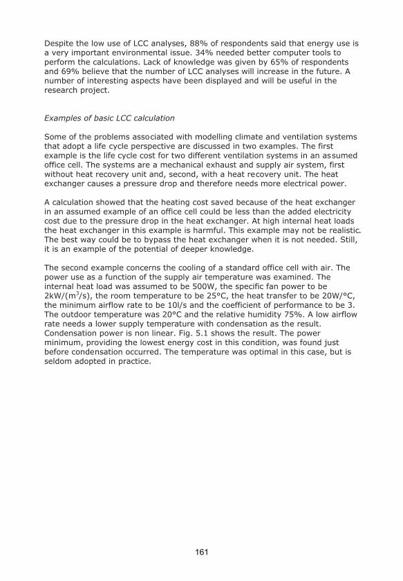
Despite the low use of LCC analyses, 88% of respondents said that energy use is a very important environmental issue. 34% needed better computer tools to perform the calculations. Lack of knowledge was given by 65% of respondents and 69% believe that the number of LCC analyses will increase in the future. A number of interesting aspects have been displayed and will be useful in the research project.

Examples of basic LCC calculation

Some of the problems associated with modelling climate and ventilation systems that adopt a life cycle perspective are discussed in two examples. The first example is the life cycle cost for two different ventilation systems in an assumed office cell. The systems are a mechanical exhaust and supply air system, first without heat recovery unit and, second, with a heat recovery unit. The heat exchanger causes a pressure drop and therefore needs more electrical power.

A calculation showed that the heating cost saved because of the heat exchanger in an assumed example of an office cell could be less than the added electricity cost due to the pressure drop in the heat exchanger. At high internal heat loads the heat exchanger in this example is harmful. This example may not be realistic. The best way could be to bypass the heat exchanger when it is not needed. Still, it is an example of the potential of deeper knowledge.

The second example concerns the cooling of a standard office cell with air. The power use as a function of the supply air temperature was examined. The internal heat load was assumed to be 500W, the specific fan power to be 2kW/(m3/s), the room temperature to be 25°C, the heat transfer to be 20W/°C, the minimum airflow rate to be 10l/s and the coefficient of performance to be 3. The outdoor temperature was 20°C and the relative humidity 75%. A low airflow rate needs a lower supply temperature with condensation as the result. Condensation power is non linear. Fig. 5.1 shows the result. The power minimum, providing the lowest energy cost in this condition, was found just before condensation occurred. The temperature was optimal in this case, but is seldom adopted in practice.

161

0

20

40

60

80

100

120

140

160

180

10 12 14 16 18

Supply air temperature / °C

Power / W

Total power

Cooling total

Cooling due to

condensation

Electrical fan

power

Fig. 5.1 Power needed to cool an office cell (depending on the supply air temperature)

Conclusions

The results of the preliminary research are simple and do not represent reality in the manner of complexity and available solutions. Nonetheless, they show ideas and options that the project will handle. The use of life cycle cost analyses is low but increasing. Therefore it will be more important to know how to perform these calculations in the future.

The state-of-the-art indicates that there is a lack of implementation of knowledge available today. A lot of climate systems do not work properly and are not as efficient as they could be. Additionally, clients and users do not have the competence or experience needed to determine if their indoor climate is good or not. A lot of money is spent on refurbishing inflexible systems and sometimes they do not work any way. This means that the research must secure the functionality of the indoor climate systems as well as providing the sector with good conditions for achieving them.

The influence on health and work performance by the indoor climate system will most likely be examined in the near future. The outcome of such research can be very difficult and expensive to implement in our indoor climate systems. Depending on the location, an increased airflow rate may result in higher work performance, a lower amount of sleep requirement at night or better health. If such effects can be proved then the systems need to be improved. It is important that the indoor climate systems built today handle the demands of tomorrow in an efficient and economical way.

162

References

Adalberth, K. (2000), Energy use and environmental impact of new residential buildings, TVBH-1012, Lund: Lund Institute of Technology.

Arditi, D.A. (1996), Life-cycle costing in municipal construction projects, Journal of Infrastructure Systems, 2, 1, pp.5-14.

Awbi, H.B. (1998), Energy efficient room air distribution, Renewable Energy, 15,pp.293-299

Besant, W.R., Eng. P. & Asiedu Y. (2000), Sizing and balancing air duct systems, ASHRAE Journal, 42, 12, pp.24.

Bull, J.W. (1993), Life cycle costing for construction, London: Blackie Academic & Professional.

Energimyndigheten (2000), Energiläget 1999, ET 81:1999, Use and production of Swedish energy, http://www.stem.se, [1 Sept. 2001] (in Swedish).

Engdahl, F. (1998), Evaluation of Swedish ventilation systems, Building and Environment, 33, 4, pp.197.

Engdahl, F. (1999), Stability of mechanical exhaust systems, Indoor Air, 9,pp.282-289.

Engdahl, F. (2000), Stability of Mechanical Exhaust and Supply Systems, Roomvent 2000, 2, pp.1207-1212.

Eurovent, (2001), Life cycle cost, Review, ed. Becirspahic, S., May 2001, s.becirspahic@eurovent-certification.com, [1 Sept. 2001].

Flanagan, R., Norman G., Meadows J. & Robinson G. (1989), Life cycle costing – Theory and practice, Oxford: BSP Professional Books.

Gustafsson, S.I. (2000), Optimisation of insulation measures on existing buildings, Energy and Buildings, 33, pp.49-55.

Imanari, T., Omori, T. & Bogaki, K. (1999), Thermal comfort and energy consumption of the radiant ceiling panel system. Comparison with the conventional all-air system, Energy and Buildings, 30, pp.167-175.

Jensen, L. (2000), Injustering av ventilationssystem – underlag för implementering, TABK—00/7058, Lund: Lund Institute of Technology (in Swedish).

Johnsson, E (2001), Projekteringsmetodik för miljöpåverkan, D57:2001, Licentiate thesis, Gothenburg: Chalmers University of Technology (in Swedish).

Matsson, L.O. (1999), LCC-jämförelser CAV, VAV och ERIC, Solna: Theorells Installationskonsult AB (in Swedish).

Milton, D.K., Glencross, M. & Walters, M.D. (2000), Risk of Sick Leave Associated with Outdoor Air Supply Rate, Humidification and Occupant Complaints,Indoor Air, 10, pp.212-221.

Sodec, F. (1999), Economic viability of cooling ceiling systems, Energy and Buildings, 30, pp.195-201.

Stetiu, C. (1999), Energy and peak power savings potential of radiant cooling systems in US commercial buildings, Energy and Buildings, 30, pp.127-138.

Sterner, E. (2000), Life cycle costing and its use in the Swedish building sector, Building Research & Information, 28, pp.387-393.

Sveriges verkstadsindustrier (1996), ENEU 94, Stockholm: Sveriges verkstadsindustrier (in Swedish).

163

Vik, T.A., (2001), Natural versus mechanical ventilation – A comparison of life-cycle cost aspects of different ventilation systems, Unpublished research project plan, Trondheim: Norwegian University of Science and Technology: http://www.ntnu.no/arkitekt/bt/ansatte/vikdrplan.html, [1 Sept. 2001].

Wargocki, P., Wyon D.P., Sundell, J., Clausein, G. & Fanger O. (2000), The effects of outdoor air supply rate in an office on perceived air quality, Sick Building Syndrome (SBS) Symptoms and Productivity, Indoor Air, 10,pp.222-236.

Weschler, C.J. & Shields, H.C. (2000), The influence of ventilation on reactions among indoor pollutants: Modelling and experimental observations, Indoor Air, 10, pp.92-100.

Yang, H., Burnett, J., Lau, K. & Lu, L. (2001), Comparing central and split air-conditioning systems, ASHRAE Journal, 43, 5, pp.36-38.

164

Optimal supply air temperature with respect

to energy use in a variable air volume

system

PAPER II

Fredrik Engdahl, Dennis Johansson (2004) Energy and Buildings, 36, pp205-218

165

166

167

168

169

170

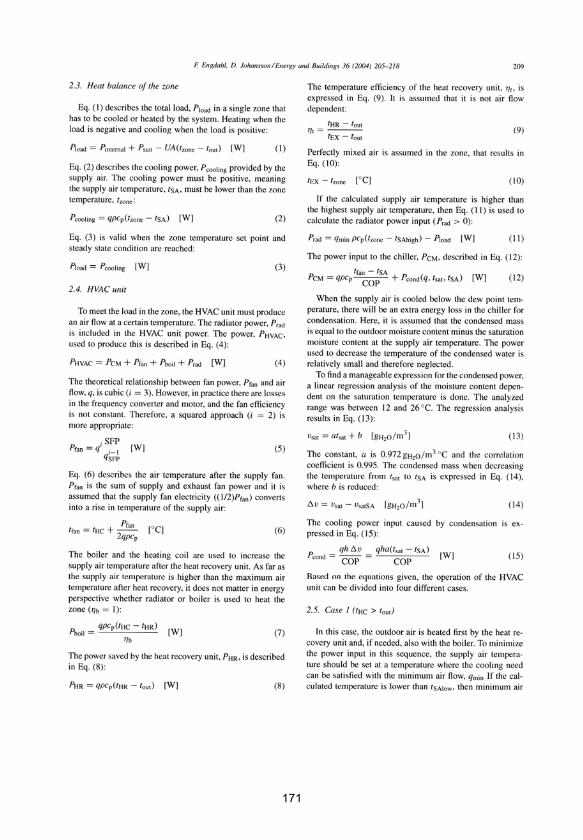
171

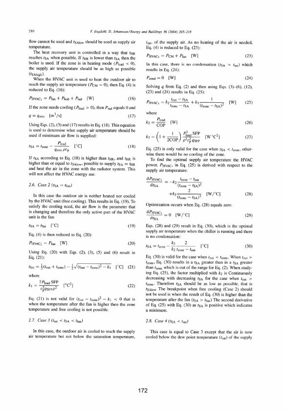
172

173

174

175

176

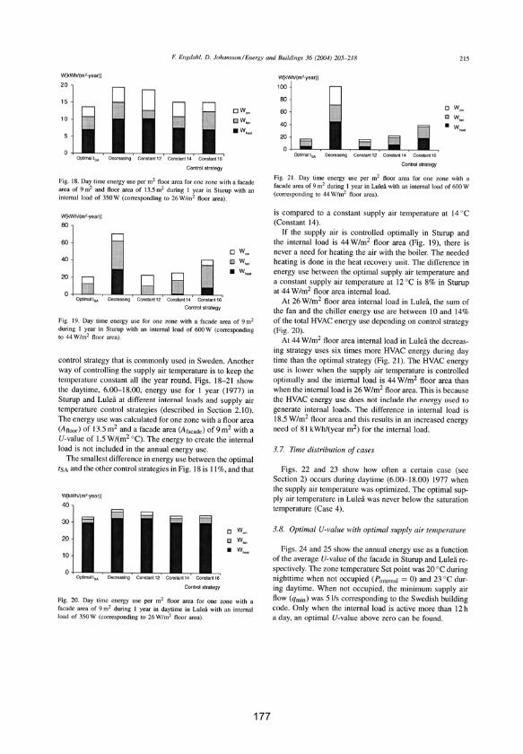
177

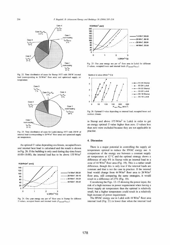
178

179

180

Optimal supply air temperature with respect

to energy use in a constant air volume

system

PAPER III

Dennis Johansson (2003) Proceedings of the 2nd international conference on building physics, Leuven, Belgium, pp699-708

181

182

1 INTRODUCTION

The main reason for using heating, ventilation and air conditioning (HVAC) systems is to satisfy users when it comes to health, indoor air quality and ther-mal comfort. The ventilation system can be either a variable air volume system (VAV) or a constant air volume system (CAV). A VAV system satisfies the health and indoor air quality criterion by supplying a minimum amount of air flow based on national regu-lations and standards. The thermal comfort is satis-fied by increasing the airflow rate when there is a cooling need and the heating need is satisfied by ra-diators. The CAV system can use an airflow rate de-termined by the health and indoor air quality. In that case, the thermal comfort is satisfied by radiators and a radiant or convective chilled surface such as a chilled ceiling or chilled beams. A CAV system can also provide a higher airflow rate to avoid the need for other cooling equipment. In that case, the heating radiators must compensate in rooms that are too cold.

In this paper, a CAV system that uses a low amount of airflow to satisfy the health and indoor air quality requirements is considered, together with heating radiators and chilled beams, to provide the correct indoor temperature for a zone in an office building. The objectives of this paper are to show a method for an optimal supply air temperature with

regards to energy use and to analyse the energy sav-ings potential when the optimal supply air tempera-ture is applied to a 100% outside air CAV system in a northern European climate.

Depending on the supply air temperature, the power used by the HVAC unit to produce the cool-ing or heating will differ. The total energy use will depend on the efficiencies of the components such as the specific fan power (SFP) value, temperature efficiency of the heat recovery unit and the chiller coefficient of performance (COP). Other factors that affect the energy use are the internal heat load, the temperature set points in the zones of the building, the outdoor air temperature and the average U-value of the building envelope.

The supply air temperature is usually controlled to be constant all the year round or decrease when the outdoor temperature increases, which is called de-creasing strategy further on. Energy calculations are made for some constant supply air temperatures, one example of the decreasing strategy and the optimal supply air temperature. The energy use is divided into three parts, the fan’s electrical energy, heating energy and cooling energy. The heating and cooling energies are either used in the HVAC unit or by the radiator or chilled beams in the zones of the building (the office cells).

In order to find a practically applicable theory and a general comparison of the energy use, a number of

Optimal supply air temperature with respect to energy use in a constant air volume system

D. Johansson Department of Building Physics, Lund University, Sweden

dennis.johansson@byggtek.lth.se

ABSTRACT: As a general rule, the built environment in the EU uses about 40% of the total energy use. A major part of this is used to provide buildings with the necessary heating and cooling. The energy use of a building can be decreased by proper controlling of the ventilation and indoor climate system. One way to de-crease the energy use is to control the supply air temperature. This paper presents a method for an optimal supply air temperature regarding energy use for a ventilation system with constant air volume (CAV). A one-zone office with a CAV system, heating radiators and chilled beams was considered. The optimisation was done by minimising the sum of the different powers to heat the air, heat the radiators, cool the air, cool the chilled beams, run the fan and condense the vapour when the air supply air temperature was cooled below the dew point temperature. The energy saving potential was also analysed when the optimal supply air tempera-ture is applied in a northern European climate. The annual energy use can be decreased significantly if the supply air temperature is optimised. An optimised supply air temperature should be possible with the control-lers available on the market but the implementation of such a control strategy requires further research.

183

assumptions and limitations are made. The energy use is calculated from hourly temperature and hu-midity data from three different climates in Sweden. The theory is based on steady state calculations. No night cooling is considered. Heat, cooling and elec-tricity are treated as equal and no economical as-pects are taken.

There is a lack of general knowledge and theoreti-cal approach regarding the influence from supply air temperature in CAV systems using only outside air. Most research has been done on VAV systems that uses return air. Most often, focus is on the propor-tions between return air and outdoor air (Stanke, 1998) in order to make it work in practice and to re-duce the energy use. In many offices and premises in northern Europe, buildings need to be cooled for a major part of the year because the buildings have in-ternal heat loads, are exposed to solar radiation and are insulated. However, the outdoor air enthalpy is usually lower than the zone air enthalpy and there-fore returning the exhaust air will only reduce the energy use a small amount. Hittle (1997), probably referring to the USA, pointed out that most VAV systems do not include any heating function in the main air-handling unit. In northern Europe, heating of the supply air is more common and with a 100% outdoor air system in the northern climates, heating of the supply air is a necessity.

Zaheer-Uddin and Zheng (1994) have shown that there is an optimal supply air temperature in a cli-mate where the relative humidity is high and return air is used. The study did not include heating of out-door air. In their case study (1996) they saved 20% of the energy use by an increase of the amount of outdoor air in a system that used return air. Norford et al. (1986) simulated an office building in New Jersey. The energy use was calculated for different constant supply air temperatures and a supply air temperature decreasing with increased outdoor tem-perature. By changing the supply air temperature, the energy use was reduced by 10% in winter time and between 11% and 21% in summer time. Xingiao et al. (2000) showed that on-line controlling of the supply air temperature could decrease the energy use significantly.

Engdahl (2002) and Johansson (2002) studied op-timal supply air temperature for a VAV system that uses only outdoor air. In South Sweden, savings of 8% was possible with an optimal supply air tempera-ture, but this would increase if the internal heat load was not constant. They also found that condensation of the moisture in the supply air should be avoided in almost all cases to decrease the energy use and that more insulation decreases the energy use if the office is not used 24 hours per day.

2 METHOD

In this study, only one zone in an office is analysed with some discussions about several zones. In a zone, which can be a cell, the indoor temperature set point, the outdoor climate and the internal load is given, from which the supply air temperature with the lowest power need is determined. The HVAC system, which provides the office cell with air and thermal comfort, uses only outdoor air. A schematic of the HVAC system and the cell is given in Figure 1.

Exhaust fan

H

eat re

covery

unit

Supply fan

Heating c

oil

Coolin

g c

oil

Zone

Outdoor air, tout

Exhaust air

Pbeam Prad

tccoilthr thcoil

PhcoilPccoil

tsa

tex

Figure 1. The studied HVAC system and the office cell.

The supply air is preheated by the heat recovery unit, cooled if necessary in the cooling coil and hea-ted if necessary in the heating coil. To get the heat balance of the zone, heating or cooling is added by the radiators or the chilled beams in the zone.

The optimisation assumes that the internal heat load is given at a given time which is relevant since the purpose is to control the ventilation system and not to design the system together with the building optimally. Therefore, the energy for the internal heat load was neglected in the energy calculations.

2.1 Nomenclature

Table 1 gives the nomenclature used in this paper

184

Table 1. The nomenclature used in this paper.

Quantity Description Unit

A facade Area of zone towards outdoors m²

A floor Floor area of zone m²

COP Coefficient of performance for chiller -

c p Specific heat of air at constant

pressure

J/(kg·K)

dt fan Supply air temperature increase

caused by the supply air fan

K

h Condensation entalphy of

condensation water

J/g

P beam Power input to chilled beams W

P ccoil Power input to cooling coil W

P cm Power input to cooling machine W

P cond Power input to condense

oversaturated water in supply air

W

P fan Power input to fans W

P in Internal heat load in zone W

P hcoil Power input to heating coil W

P hvac Power input to heating ventilation

and cooling

W

P load Cooling power needed by the zone W

P rad Power input to radiators W

q Airflow rate m³/s

RH Relative humidity -

SFP Specific fan power kW/(m³/s)

t balance Balance temperature where the air

meets the cooling need of the zone

without chilled beams or radiators

°C

t ccoil Air temperature after cooling coil °C

t ex Exhaust air temperature °C

t hcoil Air temperature after heating coil °C

t hr Air temperature after heat recovery

unit

°C

t out Outdoor temperature °C

t sa Supply air temperature °C

t sa,max Maximum supply air temperature °C

t sa,min Minimum supply air temperature °C

t sat Saturation temperature for moisture °C

t zone Zone temperature °C

U U-value of the envelope towards

outdoors

W/(m²·K)

v out Moisture content in outdoor air g/m³

v sat,sa Saturation moisture content in air at

t ccoil

g/m³

boil Efficiency of boiler for air heating -

rad Efficiency of radiator system -

t Temperature efficiency of the heat

recovery unit

-

Density of air kg/m³

2.2 Assumptions and limitations

A number of assumptions and limitations have been made:

No return air is present.No condensation is assumed in the chilled beams according to practice, which means that conden-sation can occur only in the cooling coil. If RH would be very high, this system would not work. A perfect working control system is assumed. The heating and cooling coil are not working at the same time and the radiators and the chilled beams are working one at a time. The zone tem-perature is kept constant. In the energy use calculations, the supply air tem-perature varies between 12°C and 20°C. Some practical systems do not handle those low supply air temperatures. In the energy calculations, it is assumed that there is no thermal storage in the building. The absolute energy use would differ with thermal storage but the advantages and disadvantages with different control strategies should remain. Infiltration in the building is neglected as well as leaking ducts.The exhaust temperature is equal to the zone temperature which requires perfectly mixed air in the zone. In reality, the ceiling temperature, where the air is extracted, is often higher, which results in an underestimation of the heat recovery.In the energy calculations no solar radiation is in-cluded. Solar gain can be treated as a part of the internal load, which then will vary over time. The optimisation of the supply air temperature would not be affected, but the energy use examples would differ with solar gain.The heat recovery unit is only used to save heat. It would be possible to save cooling energy when the exhaust temperature is lower than the outdoor temperature, which seldom occurs in Sweden. The boiler efficiency, boil, and the radiator sys-tem efficiency, rad, is set to 1. The water pump energy is neglected as well as the influence from temperature levels in the water system. The temperature efficiency of the heat recovery unit, t, is assumed to be constant and the supply and exhaust airflow rates are assumed to be equal. The COP of the chiller is assumed to be constant. The specific heat, cp, is assumed to be constant as well as the density, . A temperature dependent density would affect the fan power by approxi-mately 1%. Since the flow is not varied, the air properties will have a small effect on the optimi-sation.To simplify the model, all types of energies are valued equally.

185

2.3 Power balance

The supply air temperature may not exceed or fall below certain values otherwise the supply air will not be mixed in the zone (Equation 1).

max,min, sasasa ttt (1)

The cooling power needed by the zone is ex-pressed in Equation 2. Solar gain has to be included in the internal heat load.

outzonefacadeinload ttAUPP (2)

This needed cooling power must be provided by the HVAC system, which includes the thermal en-ergy from the air, the chilled beams and the radia-tors. Equation 3 describes the cooling power which is provided to the zone.

rad

radbeamsazonepload

PPttcqP (3)

In Equation 3, only one of Pbeam and Prad is pre-sent described in Equations 4 and 5.

If 0beamP , then 0radP (4)

If 0radP , then 0beamP (5)

In turn, power must be provided to the HVAC system according to Equation 6.

radcmhcoilfanhvac PPPPP (6)

In Equation 6, Pfan is given by Equation 7, Phcoil

by Equation 8 and Pcm by Equation 9. Prad can be solved from Equations 2-5.

SFPqPfan (7)

boil

hrfansaphcoil

tdttcqP (8)

COP

PPP ccoilbeam

cm (9)

When Phcoil > 0, it assumed that Pccoil = 0 and therefore thr = tccoil. Pbeam can be solved from Equa-tions 2-5. dtfan is given by Equation 10 where it is approximated that half of the fan power converts to heat in the supply air. Pccoil is given by Equation 11.

p

fanfan

cq

Pdt

2

1 (10)

COP

P

COP

dtttcqP condfansaout

pccoil (11)

Equation 11 is only valid when Pccoil > 0. Pcond is the power to condense the vapour from the supply air when it is cooled below the dew point. It is as-sumed that the supply air is saturated after the cool-ing coil just before the supply fan. Equation 12 gives the condensation power.

sasatoutcond vvhqP , (12)

Part of the air heating is done by the heat recovery unit, of which Equation 13 defines the temperature efficiency.

outex

outhrt

tt

tt (13)

It is assumed that the air is perfectly mixed, which results in Equation 14 for a single zone system.

zoneex tt (14)

The problem is to optimise Phvac according to Equation 6. Phvac(tsa) is a stepwise linear function with a number of conditions. Therefore, it is not ap-plicable to differentiate the function, equal it to zero and thereby find the optimum. Instead, a numerical approach is used to find the optimal supply air tem-perature.

2.4 Control strategies

In the energy calculations to find the benefit from optimal supply air temperature, comparisons has been made with 12, 14, 16, 18 and 20°C constant supply air temperature and for a supply air tempera-ture, which decreases with increasing outdoor tem-perature according to Fig 2. Usually in Sweden, the supply air temperature in CAV systems in offices is set to about 18°C. The decreasing strategy is seldom used for CAV systems, however it is more common with VAV systems.

tsa/°C

10

12

14

16

18

20

5 10 15 20 25

tout/°C

Figure 2. The supply air temperature as function of outdoor temperature for the denoted “decreasing strategy”.

186

2.5 Outdoor climates

The climate data used are hourly data of outdoor temperatures and relative humidity for three location in Sweden from 1991 to 2001. All temperature data are collected from SMHI (Swedish Meteorological and Hydrological Institute). Figure 3 shows the an-nual temperature frequency for Lund, which is lo-cated in South Sweden, 55°42’N, 13°11’E, 40 m above sea level. Lund has an average outdoor tem-perature of 8.4°C and a median temperature of 7.8°C. Figure 4 shows the annual temperature fre-quency for Frösön in central Sweden at 63°11’N, 14°30’E and 360 m above sea level. The average temperature was 2.9°C and the median temperature 2.7°C. Finally, Figure 5 shows the annual tempera-ture frequency of Kiruna in North Sweden, 67°51’N, 20°14’E, 505 m above sea level, with the average temperature of –0.7°C and the median temperature of –0.4°C.

Annual temperature frequency/(h/°C)

0

100

200

300

400

500

600

-40 -30 -20 -10 0 10 20 30

tout/°C

24 hour

08-18

Figure 3. The annual temperature frequency for Lund, central Sweden, for the period 1991-2001. The lower curve shows the daytime hours only.

Annual temperature frequency/(h/°C)

0

100

200

300

400

500

600

-40 -30 -20 -10 0 10 20 30

tout/°C

24 hour

08-18

Figure 4. The annual temperature frequency for Frösön for the period 1991-2001. The lower curve shows the daytime hours only.

Annual temperature frequency/(h/°C)

0

100

200

300

400

500

600

-40 -30 -20 -10 0 10 20 30

tout/°C

24 hour

08-18

Figure 5. The annual temperature frequency for Kiruna for the period 1991-2001. The lower curve shows the daytime hours only.

The relative humidity in Sweden is low if the outdoor temperature is high. Figure 6 shows the an-nual RH frequency split for three different outdoor temperature ranges in Frösön.

Annual RH frequency/(h/%)

0

10

20

30

40

50

60

20 40 60 80 100

RF/%

2.5..7.5 °C

-12.5..-7.5 °C

17.5..22.5 °C

Figure 6. The annual RH frequency in Frösön for the tempera-ture ranges given in the legend. At 17.5°C to 22.5°C, the RH is seldom above 70%.

3 RESULT

The theory for the optimal supply air temperature for a CAV system for a single zone is exemplified and the annual energy use is compared to a number of other ways to set the supply air temperature. To be able to illustrate the theory, a number of input data must be set typically for an office cell. The follow-ing data were used if nothing else is declared:

tzone = 22°C Pinternal = 300 W U = (1 W/m²·K) Afacade = 10 m² Afloor = 15 m²

t = 0.70 SFP = 2 kW/(m³·s)

187

COP = 1 RH = 80% q = 0.02 m³/s tsa,high = 20°C tsa,low = 12°C

3.1 Optimal supply air temperature

When the supply air temperature is varied in Equa-tion 6 and, in turn, Equations 7-14, Pfan is constant since the airflow rate, q, is constant. As long as boil

= rad it does not matter if the heating is provided by the radiators or the supply air. If COP is the same for both the cooling coil and the chilled beams and no condensation occurs, it does not matter if the cooling is provided by the chilled beams or the sup-ply air. The question is whether there is a cooling need or a heating need in the zone and the main dis-advantage from an energy perspective with constant supply air temperature is that the supply air can in-crease the need for cooling or heating by the chilled beams or the radiators. Figure 7 describes the opti-mal supply air temperature in different cases to-gether with the parameters which determine the op-timal supply air temperature.

0

10

20

30

-20 -10 0 10 20 30

tout/°C

t/°C

Max opt tsa

Min opt tsa

thrtout

tsat

tbalance

Figure 7. The optimal supply air temperature and the parame-ters that decides the optimal supply air temperature. Below 1°C and above 12°C, there is a range of optimal supply air tempera-tures, between the Max opt tsa and Min opt tsa, where the power requirement is the same. Between 1°C and 12°C, the Max opt tsa and Min opt tsa coincide and there is only one optimal supply air temperature.

The supply air temperature when there is balance between the cooling power needed by the zone, Pload, and the cooling power provided by the sup-ply air can be calculated with Equations 2 and 3. In that case, both Pbeam and Prad is zero. This sup-ply air temperature is shown in Figure 7, denoted as balance temperature, tbalance.

The outdoor temperature, tout, is a temperature, which makes the power to cool or heat the air zero.The dew point in the specific RH is described by the saturation temperature, tsat. This temperature is always lower than or equal to the outdoor tem-perature. The highest available temperature from the heat recovery unit is described by Equation 13 where thr must be solved for.

The balance temperature, tbalance, where Pbeam = Prad = 0 can be used as optimal supply air tempera-ture as long as the supply air temperature is higher than the saturation temperature, tsat.

When the outdoor temperature, tout, is so high that the balance temperature falls below the dew point temperature in the specific RH, added power is needed for condensation. Therefore, it is better to in-crease the supply air temperature.

When thr is lower than the balance temperature, it does not matter whether energy is put into the air or the radiators, which means that tsa should be be-tween or equal to tbalance and thr.

When the balance temperature, tbalance, is equal to tout, the supply air temperature can start to follow tout

until it reaches tsat without increased power. For the three latest statements, the optimal supply

air temperature is increased by dtfan, since the the temperature increase from the fan occurs just before the zone and is not possible to remove.

3.2 Power need

The power for heating and cooling the air, for the radiators and the chilled beams and the fan are shown in Figure 8. Here, tout has been 15°C.

0

100

200

300

400

500

600

700

5 10 15 20 25 30

tsa/°C

P/W

hvac

beam

hcoil

ccoil

rad

fan

Figure 8. The different power used by the HVAC system in the example for 15°C outdoor temperature. To the right, Pbeam and Phcoil is positive and Pccoil and Prad is zero. At 12°C, condensa-tion starts in the supply air with a change in the derivative of the Pccoil.

188

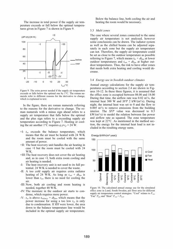
The increase in total power if the supply air tem-perature exceeds or fall below the optimal tempera-tures given in Figure 7 is shown in Figure 9.

(dP/dt)/(W /K)

0

20

40

60

80

100

-20 -10 0 10 20 30

tout/°C

below

over

+I

+II

+III

-I -II

-III -IV

-V

Figure 9. The extra power needed if the supply air temperature exceeds or falls below the optimal one by 1°C. The roman nu-merals refer to different reasons for the derivative to change, which is explained in text.

In the figure, there are roman numerals referring to the reasons for the derivative to change. The ro-man numerals with a minus sign ahead refers to a supply air temperature that falls below the optimal and the plus sign refers to a exceeding supply air temperature according to Figure 7. Heating or cool-ing the air another 1°C requires q· ·cp = 24 W.

+I: tsa exceeds the balance temperature, which means that the air must be heated with 24 W/K and the room must be cooled with the same amount of power.

+II: The heat recovery unit handles the air heating in case +I but the room must be cooled with 24 W/K.

+III: The heat recovery does not cover the air heating and, as in case +I, both extra room cooling and air heating is needed.

-I: The heat recovery unit is not used to its full po-tential. 24 W/K is needed to cover the waste.

-II: A too cold supply air requires extra radiator heating of 24 W/K. As long as tout + dtfan is lower than tsa, there is no need for cooling the air.

-III: Now, both air cooling and room heating is needed, together 48 W/K.

-IV: The moisture in the outdoor air starts to con-dense, which requires more power.

-V: tsa is above tbalance + dtfan, which means that the power increase for using a too low tsa is only due to condensation. If RH were lower, the area down to the balance temperature line would be included in the optimal supply air temperature.

Below the balance line, both cooling the air and heating the room would be necessary.

3.3 Multi zones

The case where several zones connected to the same supply air temperature is not analysed, however some conclusions can be drawn. The radiator system as well as the chilled beams can be adjusted sepa-rately in each zone but the supply air temperature can not. Therefore, the supply air temperature could be set as close to the outdoor temperature as possible referring to Figure 7, which means thr + dtfan at lower outdoor temperatures and tout + dtfan at higher out-door temperatures. Thus, the risk to have other zones that needs both extra heating and cooling would de-crease.

3.4 Energy use in Swedish outdoor climates

Annual energy calculations for the supply air tem-peratures according to section 2.4 are shown in Fig-ures 10-12. In these three figures, it is assumed that the office zone is occupied between 08.00 and 18.00 During that time, the airflow rate was 0.02 m³/s, the internal heat 300 W and SFP 2 kW/(m³/s). During night, the internal heat was set to 0 and the flow to 0.005 m³/s to remove emissions from the building interior. The SFP value was decreased to 0.5 kW/(m³/s) to model the relation between fan power and airflow rate as squared. The zone temperature was kept at 22°C. As mentioned in the method sec-tion, the energy for the internal heat load is not in-cluded in the resulting energy sums.

Energy/(kWh/(m²·year))

0

50

100

150

Optim

al

Decre

asin

g

Consta

nt

12°C

Consta

nt

14°C

Consta

nt

16°C

Consta

nt

18°C

Consta

nt

20°C

Cool

Fan

Heat

Figure 10. The calculated annual energy use for the simulated office zone in Lund, South Sweden, per floor area for different supply air temperature control strategies. “Cool” relates to Pcm,“Fan” Pfan and “Heat” Prad + Pboil.

189

Energy/(kWh/(m²·year))

0

50

100

150

Optim

al

Decre

asin

g

Consta

nt

12°C

Consta

nt

14°C

Consta

nt

16°C

Consta

nt

18°C

Consta

nt

20°C

Cool

Fan

Heat

Figure 11. The calculated annual energy use for the simulated office zone in Frösön, central Sweden, per floor area for differ-ent supply air temperature control strategies. “Cool” relates to Pcm, “Fan” Pfan and “Heat” Prad + Pboil.

Energy/(kWh/(m²·year))

0

50

100

150

200

Optim

al

Decre

asin

g

Consta

nt

12°C

Consta

nt

14°C

Consta

nt

16°C

Consta

nt

18°C

Consta

nt

20°C

Cool

Fan

Heat

Figure 12. The calculated annual energy use for the simulated office zone in Kiruna, North Sweden, per floor area for differ-ent supply air temperature control strategies. “Cool” relates to Pcm, “Fan” Pfan and “Heat” Prad + Pboil.

The possible savings compared to the best con-stant supply air temperature were 8.3%, 4,7% and 3.1% for Lund, Frösön and Kiruna respectively. The best constant supply air temperatures were 16.8°C, 16.5°C and 16.2°C respectively. The colder the cli-mate is, the less energy savings can be realised due to the higher heat demand.

In Figure 13, some different ways to run the HVAC system at night, with optimal supply air tem-perature, were tested for the location of Frösön. “Not changed” refers to the optimal case in Figure 11. If the airflow rate is not possible to decrease during nights, the energy use increases since there is a sig-nificant heating need during nights for all supplied air. The zone temperature was tested to be 18°C dur-ing night, which decreased the calculated energy use. If the airflow was high all night and the internal

heat was present as in “Occupied 24 hours”, the en-ergy use decreases significantly, at least as long as the user does not have to pay for the internal heat.

Energy/(kWh/(m²·year))

0

50

100

150

200

Not

changed

Keep flo

w

rate

at

nig

ht

18°C

at

nig

ht

Occupie

d

24 h

ours

Cool

Fan

Heat

Figure 13. Calculated annual energy use for an optimal supply air temperature at Frösön with different input data at night time (18.00-08.00). “Cool” means Pcm, “Fan” Pfan and “Heat” Prad + Pboil. “Not changed” is the same as “Optimal” in Figure 11, “Keep flow at night” means that the flow was not decreased during night, “18°C at night” means that tzone = 18°C during night and “Occupied 24 hours” means that the flow was high and the internal heat was present also at night.

3.5 Influence of parametric changes on energy use

To test the savings from an optimal supply air tem-perature, some parameters were changed in the cal-culations. In all these cases (Figures 14-18), the lo-cation has been Frösön. The office zone has been occupied between 08.00 and 18.00 in the same way as in section 3.4. Optimal supply air temperature, constant supply air temperatures of 12, 15 and 18°C and the decreasing temperature according to section 2.4 were calculated.

Figure 14 gives the total annual energy use if COP is changed. For all COPs, the optimisation de-creases the energy use significantly. The best con-stant temperature increases slightly since it is cheaper to overcool the air or the room with higher COP.

In Figure 15 the SFP value is varied. The main difference is the constant fan power. There is a slight influence from dtfan that in turn varies.

190

Energy/(kWh/(m²·year))

100

110

120

130

140

150

0.5 1 1.5 2 2.5 3

COP

Constant

12°C

Constant

15°C

Constant

18°C

Decreasing

Optimal

Figure 14. The annual total energy use (without energy for in-ternal heat) if the coefficient of performance of the chiller was changed. The calculation was made for Frösön and the office zone was occupied between 08.00 and 18.00.

Energy/(kWh/(m²·year))

100

110

120

130

140

150

0.5 1 1.5 2 2.5 3

SFP/(kW/(m³/s))

Constant

12°CConstant

15°C

Constant

18°CDecreasing

Optimal

Figure 15. The annual total energy use (without energy for in-ternal heat) if SFP was changed. The calculation was made for Frösön and the office zone was occupied between 08.00 and 18.00.

The internal heat is varied in Figure 16. Around 25 W/m² (375 W), the best constant supply air tem-perature changes to lower values depending on the higher cooling need. It indicates the internal load should be known and constant over the year to set a proper constant supply air temperature.

Figure 17 shows the variation of the U-value. With good insulation, the constant supply air tem-perature should be low and with poor insulation, the constant temperature should be high. With poor in-sulation, the savings with optimal supply air tem-perature is low.

Figure 18 gives the influence from the occupation time. If the office zone is occupied all hours, it is even more relevant to optimise the supply air tem-perature since the annual air volume is higher.

Energy/(kWh/(m²·year))

100

120

140

160

180

200

220

0 10 20 30 40 50

Pin/(W/m²)

Decreasing

Constant

18°C

Constant

15°C

Constant

12°C

Optimal

Figure 16. The annual total energy use (without energy for in-ternal heat) depending on the internal heat. The calculation was made for Frösön and the office zone was occupied between 08.00 and 18.00.

Energy/(kWh/(m²·year))

40

60

80

100

120

140

160

180

0 0.5 1 1.5

U/(W/(m²·K))

Constant

12°C

Constant

15°C

Decreasing

Constant

18°C

Optimal

Figure 17. The annual total energy use (without energy for in-ternal heat) depending on U-value of the area towards out-doors. The calculation was made for Frösön and the office zone was occupied between 08.00 and 18.00.

191

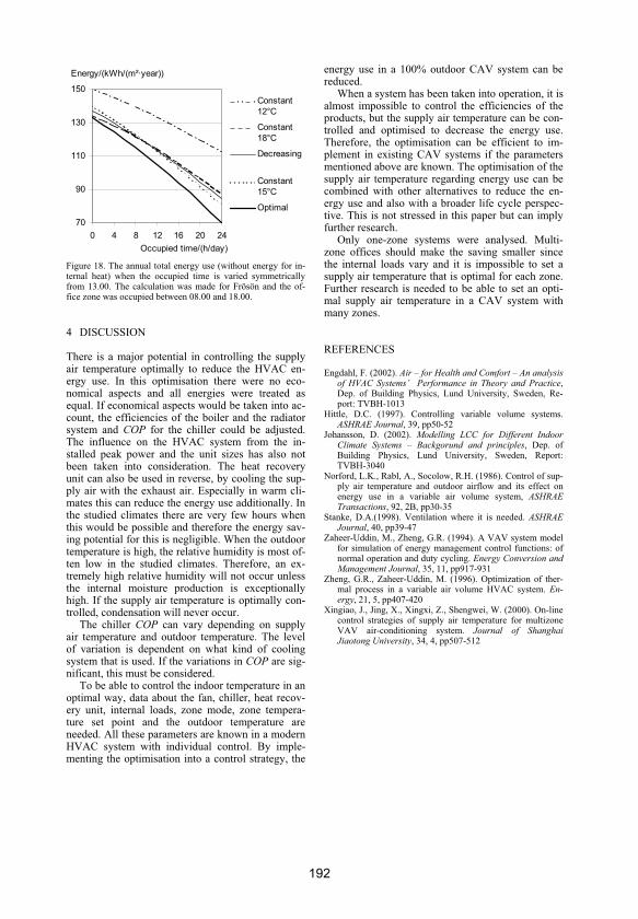
Energy/(kWh/(m²·year))

70

90

110

130

150

0 4 8 12 16 20 24

Occupied time/(h/day)

Constant

12°C

Constant

18°C

Decreasing

Constant

15°C

Optimal

Figure 18. The annual total energy use (without energy for in-ternal heat) when the occupied time is varied symmetrically from 13.00. The calculation was made for Frösön and the of-fice zone was occupied between 08.00 and 18.00.

4 DISCUSSION

There is a major potential in controlling the supply air temperature optimally to reduce the HVAC en-ergy use. In this optimisation there were no eco-nomical aspects and all energies were treated as equal. If economical aspects would be taken into ac-count, the efficiencies of the boiler and the radiator system and COP for the chiller could be adjusted. The influence on the HVAC system from the in-stalled peak power and the unit sizes has also not been taken into consideration. The heat recovery unit can also be used in reverse, by cooling the sup-ply air with the exhaust air. Especially in warm cli-mates this can reduce the energy use additionally. In the studied climates there are very few hours when this would be possible and therefore the energy sav-ing potential for this is negligible. When the outdoor temperature is high, the relative humidity is most of-ten low in the studied climates. Therefore, an ex-tremely high relative humidity will not occur unless the internal moisture production is exceptionally high. If the supply air temperature is optimally con-trolled, condensation will never occur.

The chiller COP can vary depending on supply air temperature and outdoor temperature. The level of variation is dependent on what kind of cooling system that is used. If the variations in COP are sig-nificant, this must be considered.

To be able to control the indoor temperature in an optimal way, data about the fan, chiller, heat recov-ery unit, internal loads, zone mode, zone tempera-ture set point and the outdoor temperature are needed. All these parameters are known in a modern HVAC system with individual control. By imple-menting the optimisation into a control strategy, the

energy use in a 100% outdoor CAV system can be reduced.

When a system has been taken into operation, it is almost impossible to control the efficiencies of the products, but the supply air temperature can be con-trolled and optimised to decrease the energy use. Therefore, the optimisation can be efficient to im-plement in existing CAV systems if the parameters mentioned above are known. The optimisation of the supply air temperature regarding energy use can be combined with other alternatives to reduce the en-ergy use and also with a broader life cycle perspec-tive. This is not stressed in this paper but can imply further research.

Only one-zone systems were analysed. Multi-zone offices should make the saving smaller since the internal loads vary and it is impossible to set a supply air temperature that is optimal for each zone. Further research is needed to be able to set an opti-mal supply air temperature in a CAV system with many zones.

REFERENCES

Engdahl, F. (2002). Air – for Health and Comfort – An analysis of HVAC Systems’ Performance in Theory and Practice,Dep. of Building Physics, Lund University, Sweden, Re-port: TVBH-1013

Hittle, D.C. (1997). Controlling variable volume systems. ASHRAE Journal, 39, pp50-52

Johansson, D. (2002). Modelling LCC for Different Indoor Climate Systems – Backgorund and principles, Dep. of Building Physics, Lund University, Sweden, Report: TVBH-3040

Norford, L.K., Rabl, A., Socolow, R.H. (1986). Control of sup-ply air temperature and outdoor airflow and its effect on energy use in a variable air volume system, ASHRAE Transactions, 92, 2B, pp30-35

Stanke, D.A.(1998). Ventilation where it is needed. ASHRAEJournal, 40, pp39-47

Zaheer-Uddin, M., Zheng, G.R. (1994). A VAV system model for simulation of energy management control functions: of normal operation and duty cycling. Energy Conversion and Management Journal, 35, 11, pp917-931

Zheng, G.R., Zaheer-Uddin, M. (1996). Optimization of ther-mal process in a variable air volume HVAC system. En-ergy, 21, 5, pp407-420

Xingiao, J., Jing, X., Xingxi, Z., Shengwei, W. (2000). On-line control strategies of supply air temperature for multizone VAV air-conditioning system. Journal of Shanghai Jiaotong University, 34, 4, pp507-512

192

Occupancy levels in three Swedish offices –

influence on energy use

PAPER IV

Dennis Johansson Submitted to Building and Environment 2005

193

194

Occupancy levels in three Swedish offices – influence on energy use

Dennis Johansson Building Physics Lund University

Abstract

The occupancy level in buildings is an important factor regarding demand controlled ventilation systems and energy use calculations. There is a lack of data for actual occupancy levels in offices and the question is which airflow rates should be used in energy calculations for office buildings. This study reports on measured occupancy levels in three office buildings in southern Sweden. This study also gives corrections for designing the ventilations system and calculating the fan energy use based on different occupancy level distributions. Energy use is also estimated for a demand controlled ventilation (DCV) system compared to a constant air volume (CAV) ventilation system with the occupancy level as parameter. The measured overall average occupancy rate was 15% for all time and 46% if only daytime is included. The occupancy can be approximated with binomial distributions if daytime and other time is separated.

1. Introduction

Demand controlled volume (DCV) ventilation uses a load parameter such as carbon dioxide concentration or occupancy to determine the airflow rate needed in a building at a certain time. To calculate the energy use of the ventilation fans, the specific fan power (SFP) value can be used, which expresses the fan power needed to supply 1 m³/s of air. Since the fan power varies with the flow, this SFP value must be defined at a certain air flow rate, which should be 65% of the maximum air flow rate according to methods used in Sweden (Föreningen Ventilation, 2000). To determine the needed air flow rate and the internal heat load at a specific time, the occupancy level in the building must be known, in other words the number of occupied rooms or the probability that a certain room is occupied at a certain time.

The occupancy levels are of interest in all kinds of buildings. In industry and schools, schedules can usually help to determine the occupancy. In dwellings, people have very different behaviour that is influenced by their living. Usually nights are spent at home but the evening time and the split between work and home time can look very different. Therefore, the occupancy in Swedish dwellings can be expected to be between 40 and 80% depending on work and spare time behaviour. For measuring occupancy in dwellings, occupancy sensors can be used, but questionnaires or carbon dioxide sensors could be

used instead. The problem is to decide when which rooms are occupied and by how many people.

Offices were of most interest to estimate the occupancy for because the building sector seems to prevent the dwellings from using DCV ventilation. Cell offices were chosen to avoid the problem of measuring the number of people in a room.

For offices, the occupancy varies a lot with the kind ofbusiness. Secretary work can yield almost 100% occupancy whilst field work can result in 10% occupancy in the office during daytime. Occupancy can be determined with carbon dioxide sensors, occupancy sensors or mixed gas sensors. Literature discusses control features and requirements on the system to be able to transform the sensor measurements to occupancy and needed airflow (Schell and Int-Hout, 2001). Other ways would be to send out questionnaires or analyze working schedules but that is not possible during real time operations.

The energy saving from DCV compared to constant air volume (CAV) was reported to be 50% for an auditorium space ventilated with a DCV system (Warren and Harper, 1991). An advantage of an occupancy sensor is that it can control lighting thus saving 30% in energy use (Garg and Bansal, 2000). A number of object studies showed energy savings of up to 50% (Fisk and De Almeida, 1998).

In Sweden, a base flow rate is required per floor area plus a flow rate per persons occupying the room. When there is none in a room, only the floor area dependant flow is needed. The required ventilation rates have been discussed by Boverket (2002) and Enberg (1995).

Bernard et al. (2003) measured occupancy levels in 27 French offices with occupancy sensors. Their result showed an average occupancy rate of 40% over two weeks of ten hour working days. The levels for the different offices ranged from 8 to 70%. Bernard et al. also measured the occupancy rate for 13 meeting rooms where the number of people in the room was accounted for. Here, they also used web-cams to verify the number of people. During the ten hour working days the occupied time was 16% on average, the average number of people divided by the designed number was 48% which gives an occupation level of 8% on average. They concluded that occupancy sensors were appropriate to determine whether a room is occupied but not good at determining the number of people in a room. They also underlined the importance of a correct installation of the sensors.

Bauman and McClintock (1993) reported between 70% and 75% occupancy at the nominally occupied hours of the day in US. Wang et al. (2005) report 78%

195

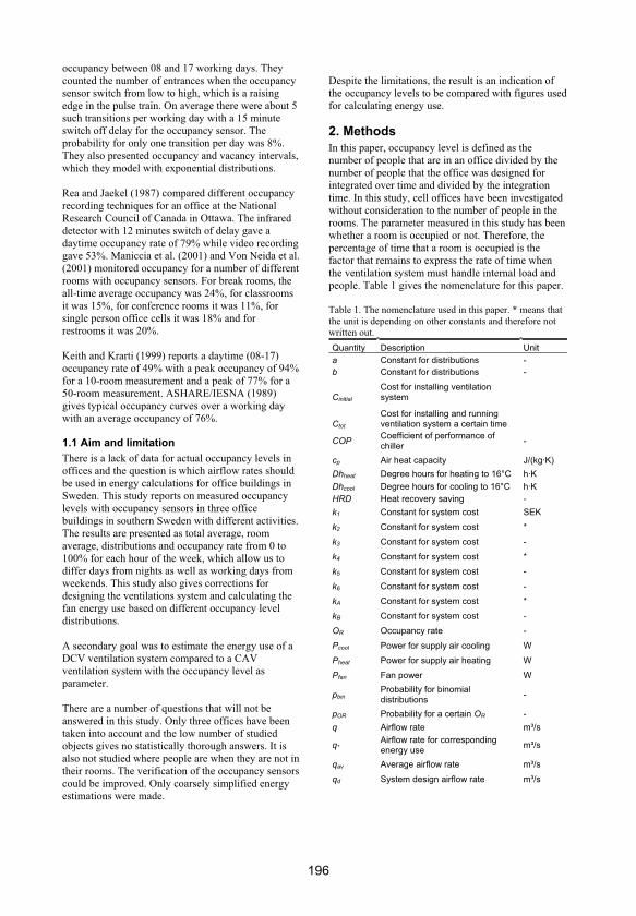
occupancy between 08 and 17 working days. They counted the number of entrances when the occupancy sensor switch from low to high, which is a raising edge in the pulse train. On average there were about 5 such transitions per working day with a 15 minute switch off delay for the occupancy sensor. The probability for only one transition per day was 8%. They also presented occupancy and vacancy intervals, which they model with exponential distributions.

Rea and Jaekel (1987) compared different occupancy recording techniques for an office at the National Research Council of Canada in Ottawa. The infrared detector with 12 minutes switch of delay gave a daytime occupancy rate of 79% while video recording gave 53%. Maniccia et al. (2001) and Von Neida et al. (2001) monitored occupancy for a number of different rooms with occupancy sensors. For break rooms, the all-time average occupancy was 24%, for classrooms it was 15%, for conference rooms it was 11%, for single person office cells it was 18% and for restrooms it was 20%.

Keith and Krarti (1999) reports a daytime (08-17) occupancy rate of 49% with a peak occupancy of 94% for a 10-room measurement and a peak of 77% for a 50-room measurement. ASHARE/IESNA (1989) gives typical occupancy curves over a working day with an average occupancy of 76%.

1.1 Aim and limitation

There is a lack of data for actual occupancy levels in offices and the question is which airflow rates should be used in energy calculations for office buildings in Sweden. This study reports on measured occupancy levels with occupancy sensors in three office buildings in southern Sweden with different activities. The results are presented as total average, room average, distributions and occupancy rate from 0 to 100% for each hour of the week, which allow us to differ days from nights as well as working days from weekends. This study also gives corrections for designing the ventilations system and calculating the fan energy use based on different occupancy level distributions.

A secondary goal was to estimate the energy use of a DCV ventilation system compared to a CAV ventilation system with the occupancy level as parameter.

There are a number of questions that will not be answered in this study. Only three offices have been taken into account and the low number of studied objects gives no statistically thorough answers. It is also not studied where people are when they are not in their rooms. The verification of the occupancy sensors could be improved. Only coarsely simplified energy estimations were made.

Despite the limitations, the result is an indication of the occupancy levels to be compared with figures used for calculating energy use.

2. Methods

In this paper, occupancy level is defined as the number of people that are in an office divided by the number of people that the office was designed for integrated over time and divided by the integration time. In this study, cell offices have been investigated without consideration to the number of people in the rooms. The parameter measured in this study has been whether a room is occupied or not. Therefore, the percentage of time that a room is occupied is the factor that remains to express the rate of time when the ventilation system must handle internal load and people. Table 1 gives the nomenclature for this paper.

Table 1. The nomenclature used in this paper. * means that the unit is depending on other constants and therefore not written out.

Quantity Description Unit

a Constant for distributions -

b Constant for distributions -

Cinitial

Cost for installing ventilation system

Ctot

Cost for installing and running ventilation system a certain time

COPCoefficient of performance of chiller

-

cp Air heat capacity J/(kg·K)

Dhheat Degree hours for heating to 16°C h·K

Dhcool Degree hours for cooling to 16°C h·K

HRD Heat recovery saving -

k1 Constant for system cost SEK

k2 Constant for system cost *

k3 Constant for system cost -

k4 Constant for system cost *

k5 Constant for system cost -

k6 Constant for system cost -

kA Constant for system cost *

kB Constant for system cost -

OR Occupancy rate -

Pcool Power for supply air cooling W

Pheat Power for supply air heating W

Pfan Fan power W

pbinProbability for binomial distributions

-

pOR Probability for a certain OR -

q Airflow rate m³/s

q*Airflow rate for corresponding energy use

m³/s

qav Average airflow rate m³/s

qd System design airflow rate m³/s

196

qd_optOptimal system design airflow rate

m³/s

qnom Flow at full occupancy m³/s

SFP Specific fan power kW/(m³/s)

tsa Supply air temperature °C

thx Temperature from heat recovery °C

tout Outdoor temperature °C

tex Exhaust air temperature °C

Wfan Fan energy use W

Wfan_avFan energy use based on average airflow rate

W

Wheat Annual energy for air heating kWh

Wcool Annual energy for air cooling kWh

Added occupancy coefficient -

tTemperature efficiency of heat recovery unit

-

Air density kg/m³

Time s

2.1 Hardware and software

The occupancy was measured with stock IR occupancy sensors for DCV systems (CALECTRO PIR-TF-25). These sensors were set up to switch on immediately if there was a hot body moving in the sensor area which occurs if there are people in the room. There is a risk that a reading person does not move. Therefore, these sensors had a 5 minute delay before switching off.

This adjustable delay adds error to the measurements. It would be possible to correct for the delay every time a room becomes empty. This was not done since the occupancy sensors can not correct for the delay in real time in a ventilation system. Additionally, the delay time is usually set higher in actual systems.

Electrically, the sensors, as most ventilation equipment in Sweden, were connected to a 24 V power source. They have an alternating switch that was connected over a voltage divider to the parallel port of a PC. According to Nyquist’s theory, the sampling frequency should be at least two times the actual variation. With no switch-on delay and 5 minutes switch-off delay, a sampling rate of four minutes was chosen to give a reasonable resolution and avoid missing any detections. Software was written in Delphi programming language to detect up to eight occupancy sensors at a time at the chosen interval for this purpose.

2.2 Measured objects

The three measured offices consisted of one municipality planning office (MPO), one university department (UD) and one industrial office (IO). In the municipality planning office, eight rooms were monitored for four weeks. The rooms were chosen randomly with the exception that all rooms were used (no vacations, long term sick leave or empty). Some

people working here have field work with controlling hygiene and animal care where they leave the building. On the other hand, some people work with administrative issues and were expected to be there almost all day.

In the University department, the staff is sometimes independent of the workplace, travels a lot and sometimes supervises students. Therefore, a low occupancy level was expected. Here, seven rooms were monitored for six weeks. The rooms were chosen the same way as for the municipality planning office.

In the industrial office, the measuring equipment was moved so that 32 rooms were monitored. Some were monitored for only two days and some for up to a week. The rooms were on different floors and in different buildings that belonged to the company. Therefore, the people working in the rooms have very different assignments making it difficult to predict the occupancy. These rooms were randomly chosen without exceptions. Therefore, a room could have been without an inhabitant. Due to the short measuring period in each set up, no statistical analysis was performed on the data from this industrial office.

In all offices, the ventilation system was a CAV system. In all rooms, it was common to have the doors opened to the corridor. Therefore, the carbon dioxide concentration was levelled out between the rooms and not used for comparisons although it was measured in the municipality planning office and the industrial office.

2.3 Influence from occupancy levels on fan energy use

Since the SFP-value has become more important for ventilation systems, it is of interest to know how to handle variable air volume (VAV) systems regarding fan energy use. The problem is that the fan power need is not linear to the airflow rate. Therefore, the actual distribution of the airflow rate influences the energy use for the fans. An approach would be to use the average airflow rate to calculate the fan energy use instead of an exact approach.

The fan power need for a certain airflow rate can be simplified to Equation 1 (Jensen, 2000) based on the fact that the power is the air flow rate times the pressure drop divided by the fan efficiency. If the efficiency is constant and the pressure drop is squared, the kB is 3. In an actual case, there are linear pressure drops involved in the form of filters and heat exchanger and the fan efficiency is not constant. It seems to be more reasonable to set kB = 2. The fan energy use is given by Equation 2. The q( ) can be taken from probability distribution data. If the average airflow rate is used in the calculations, the fan energy

197

use is expressed by Equation 3. In Equation 2, kA is supposed to be constant. Therefore, Equation 4 expresses the ratio between the actual fan energy use and the fan energy use if the average airflow rate were used in the calculation.

BkAfan qkP )()( (1)

dqkW BkAfan )( (2)

BB kmA

kmAfan qkdqkW (3)

B

B

km

k

avfan

fan

q

dq

W

W )(

_

(4)

Equation 4 is given for some simple probability distributions to show the error by using average airflow rate and to make corrections possible. Instead of the average airflow rate qm, it could be possible to use a corrected constant airflow rate q* instead of qm

determined in the way that the fan energy use will be correct.

Based on the fact that people generally work daytime and avoid work other time, a two point distribution according to Figure 1, 2 and 3 was evaluated. In Figure 1, the air flow rate was supposed to be zero when the occupancy level was zero. In Figure 2, the airflow rate was supposed to be 0.33 when the occupancy was zero, corresponding to the Swedish requirements (Boverket, 2002) of 0.35 l/(s·m²) + 7 l/person and an assumption of 0.1 person/m². The maximum flow was normalized to 1 for this case as well as for the rest of the cases. In Figure 3, the high point in the distribution was fixed to 1. The case with the base flow of 0.33, that means no occupancy, can be found at a = 0.33. Rectangular distribution was calculated with the edges in a and b. The base flow 0.33 situation is when a = 0.33.

pOR

pOR pOR

OR0 1a

0

b

1

1-b

OR0 1a

0

b

1

1-b

0.33

OR0 1a

0

b

1

1-b

Figure 1,2 and 3. Analyzed distributions regarding added fan energy use depending on non uniform airflow rate.

If the probability that an individual room is occupied is pbin and assumed constant and if it is assumed that there is no correlation between the rooms, the distribution will be binomial with n as the number of rooms. It is not reasonable to believe that there is no correlation since people tend to work at daytime and not at other time but if the occupancy distribution is split into daytime, which means 08-18, Mon-Fri, and other time, which means the rest of the week, it could be reasonable to believe that the distribution is binomial. Another issue is that the probability that individual rooms are occupied is not constant for all rooms. The binomial distribution is shown by Figure 4.

pOR

0

0.1

0.2

0.3

0.4

0.5

0 0.25 0.5 0.75 1OR

pbin=0.5,

n=2

pbin=0.1,

n=10

pbin=0.5,

n=10

pbin=0.5,

n=100

Figure 4. The binomial distribution based on the constant probability that a person is in a room and the number of rooms. The number of occupants is normalized to OR.

198

Wf an/Wf an av

1

1.05

1.1

1.15

1.2

1.25

1.3

1.35

0 0.5 1

b

a=1.00

a=0.93

a=0.87

a=0.80

a=0.73

a=0.67

a=0.60

a=0.53

a=0.46

a=0.40

Figure 5. The error by using constant average airflow rate for a two-point distribution in 0.33 and a according to Figure 2. The curves have the same order as in the legend for all Figures in the rest of this section.

q*/qav

1

1.05

1.1

1.15

1.2

0 0.25 0.5 0.75 1b

a=1.00

a=0.93

a=0.87

a=0.80

a=0.73

a=0.67

a=0.60

a=0.53

a=0.46

a=0.40

Figure 6. The airflow rate error according to Figure 5.

Figure 5 gives the ratio between the actual fan energy use and the fan energy use with a constant airflow rate for kB = 2 when the distribution of Figure 2 was used. Figure 6 gives the ratio between the q* and qav which can be used to compensate the average airflow rate to obtain a fan energy use without the integration calculation. It can be seen that the q*/qav is the square root of the Wfan/Wfan_av, which is explained by Equation 1. Therefore, the q*/qav is not shown for the other cases. If kB = 3, the q*/qav is the cubic root of the Wfan/Wfan_av.

For a = 1, the error is expected to be highest since the distance between the two present occupancy levels is highest. For a = 0.33, the error is zero since the distribution for the averaged case is exactly the same. The same discussion can be applied if b = 0 or b = 1 since the distribution becomes a one-point distribution.

Wf an/Wf an av

0

10

20

30

40

50

0 0.2 0.4 0.6 0.8 1

b

Figure 7. The error by using constant average airflow rate for a two-point distribution in 0 and a according to Figure 1.

Figure 7 gives the fan energy error for the distribution according to Figure 1 were one of the two points is zero. By that, the relative error does not depend on a.

Figure 8 gives the fan energy error if kB = 3, similar to Figure 5 for the distribution according to Figure 2. A higher kB results in a higher error and is not shown for the rest of the cases since it is not a practical value.

Wf an/Wf an av

1

1.5

2

2.5

0 0.25 0.5 0.75 1

b

a=1.00

a=0.93

a=0.87

a=0.80

a=0.73

a=0.67

a=0.60

a=0.53

a=0.46

a=0.40

Figure 8. The same data as Figure 5 with the distribution according to Figure 2 except that kB = 3 instead of 2 as in the rest of the cases.

Wf an/Wf an av

1

1.5

2

0 0.25 0.5 0.75 1

b

a=0.0

a=0.1

a=0.2

a=0.3

a=0.4

a=0.5

a=0.6

a=0.7

a=0.8

a=0.9

Figure 9. The error by using constant average airflow rate for a two-point distribution in a and 1 according to Figure 3.

199

In Figure 9, the distribution of Figure 3 was used with one of the points in 1 and the other in a. If a is small and b is close to one, the relative error becomes large even though the absolute error is not. If a = 1, the error is zero due to the resulting one-point distribution and therefore excluded from the graph.

Wf an/Wf an av

1

1.05

1.1

1.15

1.2

1.25

1.3

1.35

0 0.2 0.4 0.6 0.8 1

a

b=1.0

b=0.9

b=0.8

b=0.7

b=0.6

b=0.5

b=0.4

b=0.3

b=0.2

b=0.1

Figure 10. The fan energy use error by using constant average airflow rate for a rectangular distribution with edges in a and b where b > a.

Wf an/Wf an av

1

1.05

1.1

1.15

1.2

1.25

1.3

1.35

0 0.25 0.5 0.75 1pbin

1

2

4

8

16

32

64

128

Figure 11. The fan energy use error by using binomial distribution with a zero occupancy airflow rate of 0.33. The legend shows the number of rooms.

A rectangular distribution with edges in a and bresults in the error shown in Figure 10 where it is a condition that b > a. If b = a, the distribution is one-point with zero error. It can be shown by use of centre of area of the distribution that the error must be 4/3 if a = 0 and b > 0 which correspond to the figure.

Figure 11 gives the error if a binomial distribution was used with different single probabilities and number of rooms. A base airflow rate of 0.33 was used when the occupancy was zero. This distribution is discrete. The case with one room corresponds to Figure 5 with a = 1, since a binomial distribution with one room is a two-point distribution. Figure 12 gives the same situation but with no airflow rate at zero occupancy.

Wf an/Wf an av

0

5

10

15

0 0.25 0.5 0.75 1pbin

1

2

4

8

16

32

64

128

Figure 12. The fan energy use error by using binomial distribution with no air flow rate at zero occupancy. The legend shows the number of rooms.

The cost of a ventilation system can be expressed by Equation 5. The two first terms is the initial cost, Cinital, to buy and mount the system. The third term is the running costs assumed to be fan electricity. Here, qd is a design flow that is proportional to the cross section area of the air handling unit and the duct system. The proportional constant is the cross section average speed. The electrical power needed is assumed to depend on the cross section average speed powered by the constant k6.

6

5

3

)(421 k

d

k

kdtot

q

dqkqkkC (5)

The constant k3 describes how the cost is influenced by the component sizes. Data show that it is close to 1 for air handling units but for duct system components, it is below 1 (Johansson, 2005, Wikells, 2003). The constants k5 and k6 both describes the influence on fan power from the airflow rate and it is reasonable to set k5 = k6 + 1 since the airflow rate is multiplied by pressure drop to obtain the fan power.

Differentiating Equation 5 due to qd gives Equation 6. Setting Equation 6 to zero, and resolving for qd gives the optimal qd, see Equation 7.

0)( 5

63 146

123

dq

qkkqkkdq

dC

k

kd

kd

d

tot

(6)

635

1

23

46, )(

kkk

optd dqkk

kkq (7)

If qd,opt is inserted in Equation 5, the cost for the optimal solution will be according to Equation 8.

200

6

3

23

46

21

23

46

4

23

462

1

1)(

)(

)(

)(

63

3

5

63

6

5

5

63

3

5

k

kdq

kk

kk

kkdqkk

kk

dq

kdqkk

kkk

kC

kk

k

k

kk

k

k

k

kk

k

k

tot

(8)

If it is assumed that k1 = 0, the 1 in the last brackets corresponds to the initial cost and the ratio k3/k6

corresponds to the running costs which give a constant ratio between the initial cost and the total cost according to Equation 9.

6

31

1

k

kC

C

tot

initial (9)

If k3 = 1 and k6 = 1, which means that the power is the square of the flow rate for a certain system, the initial part of total cost is 67%. The integral in Equation 8 is known from Equation 2 so the error on the fan energy use can be used also regarding the costs but the total cost is only influenced by the error in fan energy use with a scale factor given by Equation 9.

Equation 7 also shows that the error in optimal design flow compared to a calculation with a constant average flow is the square root of the error for a certain system design with k3 =1 and k6 = 1.

2.4 Energy saving potential

Estimations of the annual energy use to heat and cool the air and to run the fan has been performed. The aim was to compare the energy use to a CAV system. Energy use for heating and cooling the supply air to constant supply air temperature of 16°C was estimated for two different outdoor climates in Sweden, Malmö and Kiruna. A heat recovery unit was assumed to be installed with a temperature efficiency, t, of 70%. The power needed to heat the supplied air is given by Equation 10. The temperature of the supply air after the heat recovery unit is given by Equation 11. Freezing in the heat exchanger was neglected although it can be expected to increase the saving of heating energy in northern Sweden from DCV ventilation since there will be more heating energy. In southern Sweden, temperatures in the exhaust air leaving the heat recovery unit are usually over the freezing point also in winter time.

The power to cool the air is given by Equation 12 where it was assumed that there was no condensation of water since this is very rare in these outdoor climates (Engdahl and Johansson, 2004). The annual energy need for heating and cooling the air can then be expressed by Equations 13 and 14 where the degree hours are used for both cooling and heating with the limit temperature as the same as the supply air temperature, 16°C. The heating need must be corrected with HRD due to the heat recovery unit, se Equation 15. The heat from the fan to the supply air was neglected. The opportunity to save cooling energy with the heat recovery unit was also neglected since it is possible only a few hours per year in Sweden.

hxsapheat ttqcP hxsa tt (10)

outex

outhxt

tt

tt (11)

COP

ttqcP saoutp

cool saout tt (12)

heatpheat DhqcHRDW (13)

COP

DhqcW coolp

cool (14)

heat

hxsa

Dh

ttHRD hxsa tt (15)

Since the power for heating and cooling is linear to the airflow rate, the average flow of an office can be used where it was assumed that the variations in airflow rate were the same all the year. Otherwise, it could affect the ratio between heating and cooling. The temperature variation of the day was also neglected. Since the occupancy is lower at nights while it is colder, more heat would be saved by use of DCV ventilation if the variation would have been simulated.

If not needed, the t was decreased so that thx = tsa.The COP, and cp were assumed to be constant at 2.5, 1.2 kg/m³ and 1000 J/(kg·K) respectively. tex has been 22°C. The outdoor climate regarding number of degree hours to the limit of 16°C and average temperatures for some locations is given in Table 2. The temperatures for a typical year were collected from the software Meteonorm (Meteotest, 2003).

The SFP-value is here defined by Equation 16, where qnom refers to the highest of supply and exhaust airflow rate. Usually they are about the same. The flow must be variable for the DCV system. To handle that, correction were applied by the use of q*/qnom to estimate the electrical power need for the fans. In theory, the power need for the fan should be in cubic relation to the flow, but measurements fit better with a

201

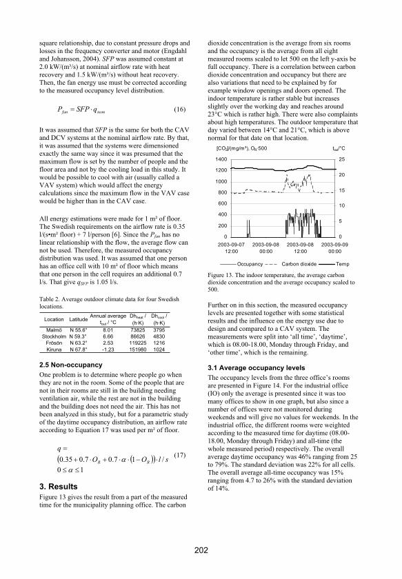
square relationship, due to constant pressure drops and losses in the frequency converter and motor (Engdahl and Johansson, 2004). SFP was assumed constant at 2.0 kW/(m³/s) at nominal airflow rate with heat recovery and 1.5 kW/(m³/s) without heat recovery. Then, the fan energy use must be corrected according to the measured occupancy level distribution.

nomfan qSFPP (16)

It was assumed that SFP is the same for both the CAV and DCV systems at the nominal airflow rate. By that, it was assumed that the systems were dimensioned exactly the same way since it was presumed that the maximum flow is set by the number of people and the floor area and not by the cooling load in this study. It would be possible to cool with air (usually called a VAV system) which would affect the energy calculations since the maximum flow in the VAV case would be higher than in the CAV case.

All energy estimations were made for 1 m² of floor. The Swedish requirements on the airflow rate is 0.35 l/(s•m² floor) + 7 l/person [6]. Since the Pfan has no linear relationship with the flow, the average flow can not be used. Therefore, the measured occupancy distribution was used. It was assumed that one person has an office cell with 10 m² of floor which means that one person in the cell requires an additional 0.7 l/s. That give qSFP is 1.05 l/s.

Table 2. Average outdoor climate data for four Swedish locations.

Location LatitudeAnnual average

tout / °C

Dhheat /

(h·K)

Dhcool /

(h·K)

Malmö N 55.6° 8.01 73825 3795

Stockholm N 59.3° 6.66 86626 4830

Frösön N 63.2° 2.53 119225 1216

Kiruna N 67.8° -1.23 151980 1024

2.5 Non-occupancy

One problem is to determine where people go when they are not in the room. Some of the people that are not in their rooms are still in the building needing ventilation air, while the rest are not in the building and the building does not need the air. This has not been analyzed in this study, but for a parametric study of the daytime occupancy distribution, an airflow rate according to Equation 17 was used per m² of floor.

slOO

q

RR /17.07.035.0 (17)

10

3. Results

Figure 13 gives the result from a part of the measured time for the municipality planning office. The carbon

dioxide concentration is the average from six rooms and the occupancy is the average from all eight measured rooms scaled to let 500 on the left y-axis be full occupancy. There is a correlation between carbon dioxide concentration and occupancy but there are also variations that need to be explained by for example window openings and doors opened. The indoor temperature is rather stable but increases slightly over the working day and reaches around 23°C which is rather high. There were also complaints about high temperatures. The outdoor temperature that day varied between 14°C and 21°C, which is above normal for that date on that location.

[CO2]/(mg/m³), OR·500

0

200

400

600

800

1000

1200

1400

2003-09-07

12:00

2003-09-08

00:00

2003-09-08

12:00

2003-09-09

00:00

0

5

10

15

20

25

tout/°C

Occupancy Carbon dioxide Temp

Figure 13. The indoor temperature, the average carbon dioxide concentration and the average occupancy scaled to 500.

Further on in this section, the measured occupancy levels are presented together with some statistical results and the influence on the energy use due to design and compared to a CAV system. The measurements were split into ‘all time’, ‘daytime’, which is 08.00-18.00, Monday through Friday, and ‘other time’, which is the remaining.

3.1 Average occupancy levels

The occupancy levels from the three office’s rooms are presented in Figure 14. For the industrial office (IO) only the average is presented since it was too many offices to show in one graph, but also since a number of offices were not monitored during weekends and will give no values for weekends. In the industrial office, the different rooms were weighted according to the measured time for daytime (08.00-18.00, Monday through Friday) and all-time (the whole measured period) respectively. The overall average daytime occupancy was 46% ranging from 25 to 79%. The standard deviation was 22% for all cells. The overall average all-time occupancy was 15% ranging from 4.7 to 26% with the standard deviation of 14%.

202

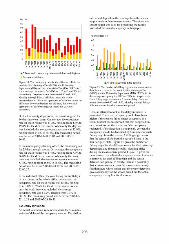
OR / %

0

10

20

30

40

50

60

70

80M

PO

1

MP

O2

MP

O3

MP

O4

MP

O5

MP

O6

MP

O7

MP

O8

MP

O A

v

UD

1

UD

2

UD

3

UD

4

UD

5

UD

6

UD

7

UD

Av

IO A

v

To

t a

v

Difference in occupancy between all-time and daytime

Occupancy all-time

Figure 14. The occupancy rate for the different cells in the municipality planning office (MPO), the University department (UD) and the industrial office (IO). ‘MPO Av’ is the average occupancy for MPO as ‘UD Av’ and ‘IO Av’ respectively. Daytime means between 08.00 and 18.00, Monday through Friday. All-time means the whole measured period. Since the upper part of each bar shows the difference between daytime and all-time, the lower and upper parts of each bar together means the daytime occupancy.

On the University department, the monitoring ran for 46 days in seven rooms. On average, the occupancy rate for these rooms was 11.2%, ranging from 4.7% to 19.8% for the different rooms. When only the daytime was included, the average occupancy rate was 32.9%, ranging from 14.8% to 48.4%. The measuring period was between 2003-03-28 15:01 and 2003-05-13 16:42.

In the municipality planning office, the monitoring ran for 25 days in eight rooms. On average, the occupancy rate for these rooms was 17.6%, ranging from 7.7% to 26.0% for the different rooms. When only the work time was included, the average occupancy rate was 53.8%, ranging from 25.0% to 78.6%. The measuring period was between 2003-08-28 12:37 and 2003-09-22 07:57.

In the industrial office, the monitoring ran for 8 days in two rooms. In the whole office, on average, the occupancy rate for these rooms was 15.2%, ranging from 3.0% to 69.6% for the different rooms. When only the work time was included, the average occupancy rate was 51.2%, ranging from 7.1% to 88.1%. The measuring period was between 2003-05-22 10:58 and 2003-05-28 10:50.

3.2 Delay influence

An actual ventilation system would use the 5 minutes switch-of delay of the occupancy sensors. The airflow

rate would depend on the readings from the sensor output made in these measurements. Therefore, the sensor output was used for presenting the results instead of the actual occupancy in this paper.

Falling edges / h

0

0.4

0.8

1.2

1.6

2

2.4

MP

O1

MP

O2

MP

O3

MP

O4

MP

O5

MP

O6

MP

O7

MP

O8

MP

O A

v

UD

1

UD

2

UD

3

UD

4

UD

5

UD

6

UD

7

UD

Av

All-time Daytime No daytime

Figure 15. The number of falling edges in the sensor output data for each room in the municipality planning office (MPO) and the University department (UD). ‘MPO Av’ is the average occupancy for MPO as ‘UD Av’ respectively. Each falling edge represents a 5 minute delay. Daytime means between 08.00 and 18.00, Monday through Friday. All-time means the whole measured period.

Here, an attempt to look at the delay influence is presented. The actual occupancy could have been higher if the sensors fail to detect occupancy in a room. Manual checks showed that that happened on rare occasions but there were no false occupancy registered. If the detection is completely correct, the occupancy should be decreased by 5 minutes for each falling edge from the sensor. A falling edge means that the sensor shifts from the occupied state to the non-occupied state. Figure 15 gives the number of falling edges for the different rooms for the University department and the municipality planning office during the measurement period. Figure 16 gives the ratio between the adjusted occupancy where 5 minutes is removed for each falling edge and the sensor detected occupancy. In reality, there is a possibility that a person enters a room for some seconds every fourth minute which means that the sensor detection gives occupancy for the whole period but the actual occupancy is very low for that room.

203

corr OR / meas OR

0

0.2

0.4

0.6

0.8

1M

PO

1

MP

O2

MP

O3

MP

O4

MP

O5

MP

O6

MP

O7

MP

O8

MP

O A

v

UD

1

UD

2

UD

3

UD

4

UD

5

UD

6

UD

7

UD

Av

All-time No daytime Daytime

Figure 16. The ratio between the detected occupancy decreased with 5 minutes for each falling edge and the detected occupancy for each room in the municipality planning office (MPO) and the University department (UD). ‘MPO Av’ is the average occupancy for MPO as ‘UD Av’ respectively. Each falling edge represent a 5 minute delay. Daytime means between 08.00 and 18.00, Monday through Friday. All-time means the whole measured period.

3.3 Correlation coefficients

Table 3. The phi correlation between all rooms in pairs. The matrix is split into the two measured objects since a full matrix would be symmetrical to save space. The correlation between the room and itself should be one which is given by the diagonal.

Room 1 2 3 4 5 6 7 8

1 1.00 0.37 0.34 0.23 0.23 0.38 0.29 -

2 0.45 1.00 0.38 0.28 0.29 0.39 0.29 -

3 0.35 0.43 1.00 0.38 0.27 0.29 0.35 -

4 0.35 0.44 0.92 1.00 0.16 0.22 0.33 -

5 0.56 0.62 0.63 0.64 1.00 0.34 0.28 -

6 0.58 0.61 0.61 0.63 0.84 1.00 0.21 -

7 0.26 0.35 0.29 0.29 0.47 0.42 1.00 -

8 0.68 0.63 0.67 0.68 0.83 0.84 0.38 1.00

University department

Municipality planning office

Phi correlation is used to test correlation between binary variables. A correlation is somewhat expected since people tend to work at daytime and stay away from work other times. On the other hand, the argument could be that field work must be done but some must take care of the office, which should tend to give a negative correlation. The phi correlation coefficients are given in Table 3 for all-time, in Table 4 for the University department and in Table 5 for the Municipality planning office. The value goes from -1 to 1 where no correlation gives the value 0. Generally, the phi correlation is lower at the University department with an average value of 0.30 compared to 0.55 at the Municipality planning office. This can be

explained by the non-regulated working times at the University department.

Table 4. The phi correlation between the rooms for the University department. The matrix is split into the daytime and other time since a full matrix would be symmetrical to save space.

Room 1 2 3 4 5 6 7

1 1.00 0.16 0.16 0.10 0.05 0.20 0.18

2 0.00 1.00 0.14 0.10 0.02 0.13 0.11

3 0.00 0.14 1.00 0.26 0.09 0.04 0.22

4 -0.01 0.18 0.20 1.00 0.02 0.06 0.25

5 -0.03 0.08 0.05 -0.01 1.00 0.18 0.13

6 0.03 0.05 0.06 0.00 0.05 1.00 0.02

7 -0.02 0.08 0.15 0.09 0.17 0.00 1.00

Daytime

Other time

Table 5. The phi correlation between the rooms for the Municipality planning office. The matrix is split into the daytime and other time since a full matrix would be symmetrical to save space.

Room 1 2 3 4 5 6 7 8

1 1.00 0.14 0.03 0.03 0.22 0.22 0.03 0.46

2 0.39 1.00 0.16 0.15 0.29 0.28 0.13 0.34

3 0.36 0.25 1.00 0.91 0.35 0.28 0.08 0.43

4 0.36 0.28 0.83 1.00 0.34 0.28 0.08 0.42

5 0.44 0.34 0.64 0.74 1.00 0.55 0.26 0.57

6 0.53 0.27 0.66 0.72 0.77 1.00 0.17 0.55

7 0.05 0.18 0.22 0.26 0.32 0.30 1.00 0.11

8 0.60 0.37 0.70 0.79 0.84 0.84 0.27 1.00

Other time

Daytime

3.4 Occupancy frequencies

pOR

0

0.2

0.4

0.6

0.8

1

0 0.5 1

OR

All meas

All bin

Day meas

Day bin

Other meas

Other bin

Figure 17. The occupancy level distribution for the University department. ‘All’ means all-time, ‘Day’ means day time and ‘Other’ means other time. ‘Meas’ aim at measured data while ‘bin’ aim at the binomial distribution based on the measured average probability and number of rooms.

204

The measured occupancy can be sorted based on how many minutes there was no people in the office up how many minutes there were exactly 8 people in measured rooms of the municipality planning office and 7 people in the measured rooms of the University department respectively. Figure 17 gives the probability for each discrete occupancy level for the University department. Figure 17 splits the occupancy in daytime and other time and also shows the binomial distribution with pbin set to the average value of the measurements and the number of rooms according to the measurements.

pOR

0

0.2

0.4

0.6

0.8

1

0 0.5 1

OR

All meas

All bin

Day meas

Day bin

Other meas

Other bin

Figure 18. The occupancy level distribution for the Municipality planning office. ‘All’ means all-time, ‘Day’ means day time and ‘Other’ means other time. ‘Meas’ aim at measured data while ‘bin’ aim at the binomial distribution based on the measured average probability and number of rooms.

In the same way, Figure 18 shows the occupancy distribution for the municipality planning office. The binomial distribution should be able to use if there is a split into daytime and other time but for the all-time case, it can be better to approximate the distribution with a 2-point distribution.

The binomial distribution is based on non-depending variables. If there is a dependence, the distribution is influenced. A positive correlation makes the distribution according to Figure 19 where data were simulated for 16 rooms of which the number of non-correlated rooms was varied from 0 to 16. If all rooms were non-correlated, the distribution is simulated to be binomial. The probability, pbin, was 0.5. Generally, the occupancy distribution tends to be flattened out if there is a correlation which is the case also in the measurements. That could depend on the fact that there is a positive phi correlation in the data. There should also be an error between the actual distribution and the binomial since all probabilities are not the same that a certain room is occupied. This was not analyzed.

pOR

0.00

0.10

0.20

0.30

0.40

0.50

0 0.5 1

OR

0

0.067

0.3

0.55

1

Figure 19. The binomial distribution based on simulated data with pbin = 0.5 in a 16 room case together with simulated data that create correlation with the same individual probability. The average phi correlation for all combinations of pairs is given by the legend. 0 corresponds 16 out of 16 non-correlated rooms, 0.067 corresponds to 12 non-correlated rooms, 0.3 to 8 non-correlated rooms, 0.55 to 4 non-correlated rooms and 1 to all rooms correlated.

3.5 Fan energy influence

If the measured occupancy distribution is used to determine the error by the average airflow rate design described in Section 2.3, the ratios of energy use and airflow rates is given by Table 6. The most realistic case is when kB = 2 and the airflow rate at zero occupancy is 33% of the nominal air flow rate.

Table 6. The error by using the average occupancy levels and airflow rates for the measured distributions.

All

time

Day-

time

Other

time

All

time

Day-

time

Other

time

Wfan/Wfan_av 4.00 1.47 8.97 4.18 1.31 27.1

q*/qav 2.00 1.21 2.99 2.05 1.14 5.20

q*/qnom 0.22 0.40 0.063 0.30 0.54 0.10

Wfan/Wfan_av 1.09 1.07 1.01 1.16 1.07 1.04

q*/qav 1.05 1.04 1.01 1.08 1.04 1.02

q*/qnom 0.43 0.57 0.35 0.46 0.67 0.35

Wfan/Wfan_av 19.10 2.50 99.7 19.1 1.85 823

q*/qav 4.37 1.58 9.98 4.37 1.36 28.7

q*/qnom 0.64 0.52 0.21 0.64 0.64 0.57

Wfan/Wfan_av 1.35 1.22 1.04 1.59 1.21 1.15

q*/qav 1.16 1.11 1.02 1.26 1.10 1.07

q*/qnom 0.47 0.61 0.35 0.54 0.72 0.37

kB=3, q = 0 at OC = 0

kB=3, q = 0.33·qnom at OC=0

University departmentMunicipality planning

office

kB=2, q = 0 at OC = 0

kB=2, q = 0.33·qnom at OC=0

The error in Table 6 would be influenced by the more narrow distribution that would be the case if the number of rooms is more than 8 and 7 respectively for the two objects. According to Equation 17, rooms can be detected as empty but the people are still in the building. Figure 20 gives the error depending on

205

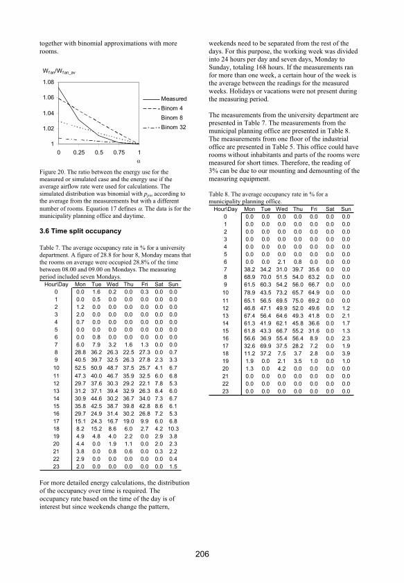
together with binomial approximations with more rooms.

Wf an/Wf an_av

1

1.02

1.04

1.06

1.08

0 0.25 0.5 0.75 1

Measured

Binom 4

Binom 8

Binom 32

Figure 20. The ratio between the energy use for the measured or simulated case and the energy use if the average airflow rate were used for calculations. The simulated distribution was binomial with ppin according to the average from the measurements but with a different number of rooms. Equation 17 defines . The data is for the municipality planning office and daytime.

3.6 Time split occupancy

Table 7. The average occupancy rate in % for a university department. A figure of 28.8 for hour 8, Monday means that the rooms on average were occupied 28.8% of the time between 08.00 and 09.00 on Mondays. The measuring period included seven Mondays.

Hour\Day Mon Tue Wed Thu Fri Sat Sun

0 0.0 1.6 0.2 0.0 0.3 0.0 0.0

1 0.0 0.5 0.0 0.0 0.0 0.0 0.0

2 1.2 0.0 0.0 0.0 0.0 0.0 0.0

3 2.0 0.0 0.0 0.0 0.0 0.0 0.0

4 0.7 0.0 0.0 0.0 0.0 0.0 0.0

5 0.0 0.0 0.0 0.0 0.0 0.0 0.0

6 0.0 0.8 0.0 0.0 0.0 0.0 0.0

7 6.0 7.9 3.2 1.6 1.3 0.0 0.0

8 28.8 36.2 26.3 22.5 27.3 0.0 0.7

9 40.5 39.7 32.5 26.3 27.8 2.3 3.3

10 52.5 50.9 48.7 37.5 25.7 4.1 6.7

11 47.3 40.0 46.7 35.9 32.5 6.0 6.8

12 29.7 37.6 30.3 29.2 22.1 7.8 5.3

13 31.2 37.1 39.4 32.9 26.3 8.4 6.0

14 30.9 44.6 30.2 36.7 34.0 7.3 6.7

15 35.8 42.5 38.7 39.8 42.8 8.6 6.1

16 29.7 24.9 31.4 30.2 26.8 7.2 5.3

17 15.1 24.3 16.7 19.0 9.9 6.0 6.8

18 8.2 15.2 8.6 6.0 2.7 4.2 10.3

19 4.9 4.8 4.0 2.2 0.0 2.9 3.8

20 4.4 0.0 1.9 1.1 0.0 2.0 2.3

21 3.8 0.0 0.8 0.6 0.0 0.3 2.2

22 2.9 0.0 0.0 0.0 0.0 0.0 0.4

23 2.0 0.0 0.0 0.0 0.0 0.0 1.5

For more detailed energy calculations, the distribution of the occupancy over time is required. The occupancy rate based on the time of the day is of interest but since weekends change the pattern,

weekends need to be separated from the rest of the days. For this purpose, the working week was divided into 24 hours per day and seven days, Monday to Sunday, totaling 168 hours. If the measurements ran for more than one week, a certain hour of the week is the average between the readings for the measured weeks. Holidays or vacations were not present during the measuring period.

The measurements from the university department are presented in Table 7. The measurements from the municipal planning office are presented in Table 8. The measurements from one floor of the industrial office are presented in Table 5. This office could have rooms without inhabitants and parts of the rooms were measured for short times. Therefore, the reading of 3% can be due to our mounting and demounting of the measuring equipment.

Table 8. The average occupancy rate in % for a municipality planning office.

Hour\Day Mon Tue Wed Thu Fri Sat Sun

0 0.0 0.0 0.0 0.0 0.0 0.0 0.0

1 0.0 0.0 0.0 0.0 0.0 0.0 0.0

2 0.0 0.0 0.0 0.0 0.0 0.0 0.0

3 0.0 0.0 0.0 0.0 0.0 0.0 0.0

4 0.0 0.0 0.0 0.0 0.0 0.0 0.0

5 0.0 0.0 0.0 0.0 0.0 0.0 0.0

6 0.0 0.0 2.1 0.8 0.0 0.0 0.0

7 38.2 34.2 31.0 39.7 35.6 0.0 0.0

8 68.9 70.0 51.5 54.0 63.2 0.0 0.0

9 61.5 60.3 54.2 56.0 66.7 0.0 0.0

10 78.9 43.5 73.2 65.7 64.9 0.0 0.0

11 65.1 56.5 69.5 75.0 69.2 0.0 0.0

12 46.8 47.1 49.9 52.0 49.6 0.0 1.2

13 67.4 56.4 64.6 49.3 41.8 0.0 2.1

14 61.3 41.9 62.1 45.8 36.6 0.0 1.7

15 61.8 43.3 66.7 55.2 31.6 0.0 1.3

16 56.6 36.9 55.4 56.4 8.9 0.0 2.3

17 32.6 69.9 37.5 28.2 7.2 0.0 1.9

18 11.2 37.2 7.5 3.7 2.8 0.0 3.9

19 1.9 0.0 2.1 3.5 1.0 0.0 1.0

20 1.3 0.0 4.2 0.0 0.0 0.0 0.0

21 0.0 0.0 0.0 0.0 0.0 0.0 0.0

22 0.0 0.0 0.0 0.0 0.0 0.0 0.0

23 0.0 0.0 0.0 0.0 0.0 0.0 0.0

206

Table 9. The average occupancy rate in % for a part of an industrial office.

Hour\Day Mon Tue Wed Thu Fri Sat Sun

0 0.0 0.0 0.0 0.0 0.0 0.0 0.0

1 0.0 0.0 0.0 0.0 0.0 0.0 0.0

2 0.0 0.0 0.0 0.0 0.0 0.0 0.0

3 0.0 0.0 0.0 0.0 0.0 0.0 0.0

4 0.0 0.0 0.0 0.0 0.0 0.0 0.0

5 0.0 0.0 0.0 0.0 0.0 0.0 0.0

6 0.0 0.0 0.0 0.0 0.0 0.0 0.0

7 0.0 0.0 0.0 0.0 0.0 0.0 0.0

8 0.0 23.3 16.7 0.0 50.0 0.0 0.0

9 46.7 50.0 46.7 0.0 93.3 0.0 0.0

10 50.0 30.0 50.0 100.0 100.0 0.0 0.0

11 53.3 43.3 0.0 71.6 96.7 0.0 0.0

12 33.3 33.3 0.0 20.0 46.7 0.0 0.0

13 46.7 50.0 0.0 43.3 46.7 0.0 0.0

14 30.0 50.0 0.0 50.0 83.3 0.0 0.0

15 50.0 50.0 0.0 76.7 86.7 0.0 0.0

16 43.3 33.3 0.0 0.0 60.0 0.0 0.0

17 0.0 0.0 0.0 6.7 3.3 0.0 0.0

18 0.0 0.0 0.0 0.0 0.0 0.0 0.0

19 0.0 0.0 0.0 0.0 0.0 0.0 0.0

20 0.0 0.0 0.0 0.0 0.0 0.0 0.0

21 0.0 0.0 0.0 0.0 0.0 0.0 0.0

22 0.0 0.0 0.0 0.0 0.0 0.0 0.0

23 0.0 0.0 0.0 0.0 0.0 0.0 0.0

3.7 Energy saving potential

Table 10 shows the estimated annual energy use per m² of floor for different cases in Malmö and Kiruna. A comparison was made without heat recovery for the Kiruna outdoor climate.

Table 10. Estimated annual energy use for 1 m² of floor divided into supply air heating, supply air cooling and fan. Malmö is in southern Sweden and Kiruna is in northern Sweden. The three bottom rows show the case without heat recovery.

System and location

Annual

heating

energy /

kWh

Annual

cooling

energy

/ kWh

Annual

fan

energy

/ kWh

Sum /

kWh

CAV-Malmö 2.50 1.91 18.4 22.8

DCV-MPO-Malmö 1.07 0.82 3.89 5.79

DCV-UD-Malmö 1.02 0.78 3.40 5.21

CAV-Kiruna 20.5 0.52 18.4 39.4

DCV-MPO-Kiruna 8.8 0.22 3.89 12.9

DCV-UD-Kiruna 8.4 0.21 3.40 12.0

CAV-Kiruna, t=0 191 0.52 13.8 206

DCV-MPO-Kiruna, t=0 82 0.22 2.92 85

DCV-UD-Kiruna, t=0 78.5 0.21 2.55 81.3

4. Discussion and conclusions

The measured occupancy levels were lower than expected which should be considered for DCV system analyses. On average, the overall occupancy was 15%, excluding vacations and holidays. On daytime, the overall average was 46%.

The question where people were when they were not in their room was not analyzed in this study, but it is reasonable to believe that for the University department, the people were outside the building a large part of the non-occupied time. At daytime, people travel, go for lunch or work from home which means that they are outside the building. The measuring period was not during an intensive teaching period and most of the measured rooms were not inhabited by teachers. On the other hand, part of the non-occupancy was due to coffee breaks and other work inside the building, eventually supplied by the same air handling unit.

For the Municipality planning office, it can also be believed that most of the non-occupancy is real since people there has a lot of field inspections of buildings, animal care and health and meetings with other departments, that are not located in the same house.

For the industrial office, it was not checked what kind of work people had since the measurements were performed in many rooms for shorter periods. Therefore, it is difficult to estimate the in Equation 17. Part of this office was an office with development and administration and part of the office was a workshop office where it can be believed that people are in the factory if not in their office rooms and thereby eventually get the ventilation air from the same air handling unit.

At other time, which for the measuring period included nights and weekends, it is reasonable to believe that almost all of the non-occupancy is real since people that work on evenings or weekends in these buildings usually seem to perform their own office work. People do not have meetings during overtime.

It is difficult to make general conclusions regarding for all buildings. If all people are present in an office and half of the staff go from their own rooms to their neighboring rooms, this measurement method will first indicate an occupancy level of 100%, then an occupancy level of 50% even if the number of people remains since the number of people in a room is not counted. In that case, people still need the same total airflow rate. On the other hand, a DCV system with occupancy sensors for cell offices has no feature to double the airflow rate in every second room. That means that people will lack air in every second room whether the airflow rate in the empty rooms is decreased or not. Therefore, there is no benefit from not decreasing the airflow rate in the empty rooms in such a situation.

A way to examine could be to look at the number of falling edges, which means how many times people

207

leave the room per hour. If people seems to run in and out, it could be reasonable to say that they are still in the building, but, according to the former paragraph, the flow will not increase somewhere else as long as they do not visit an empty room. On the other hand, with a VAV system responding to temperature or carbon dioxide, the flow could increase for example in the neighboring room if there were two people. Control of surveillance cameras, working schedules or door check system could also help if they are present, which they was not in the measured buildings.

The analysis of energy use for a system with the actual airflow rate distribution compared to the energy use for a system with constant average airflow rate show that the error by using the average airflow rate is small if there is a 33% base airflow when the room is empty but can be remarkably higher if the airflow rate at non-occupancy is zero. A kB of 2 is reasonable, which gives an error of 9% and 16% for all-time for the two objects respectively. If the occupancy is split into daytime and other time, the error decreases.

In an actual office, the number of rooms will be higher than the number of simultaneously measured rooms in this study. This should give a more narrow distribution that can be approximated with two binomial distributions, one for daytime and one for other time, or in the case of many rooms with a two point distribution. The error from an average approach should decrease with more rooms. If more rooms are present, it is also reasonable to use a ventilation system that does not handle the nominal case where the occupancy is 1.

Simplifications were made regarding the pressure drops. A more detailed approach could include thorough pressure drops calculation with information on which rooms are occupied and which are not.

If the SFP-value for a DCV system should be set to make the average fan power to the SFP-value multiplied with the nominal airflow rate, the SFP-value should be set at q*/qnom which were 43% and 46% of qnom for the analyzed buildings respectively. In Sweden, 65% is used today, which is reasonable if the airflow rate at zero occupancy is zero.

With heat recovery, most of the savings is fan electricity which is probably the most expensive kind of energy involved. The heat recovery saves a lot of heating energy and should be used. The energy use estimations were coarse and should benefit from a room power balance analysis. The assumption was made that the systems were equally designed for the DCV and the CAV system in the total energy use estimation. An optimal design would make the DCV system smaller than the CAV system and by that decreasing the initial cost partly according to Equation

8. That would result in a higher pressure drop due to the smaller system with a higher SFP-value and a higher annual energy use for fan electricity as result. Still, the initial cost is by far the major part of the total cost according to Equation 9, which means that the influence on the size and SFP-value would be small.

The measuring method is applicable since it should give the same result as an actual DCV system in cell offices with occupancy sensor. The problem with the method used is to determine the number of people in a room and where people are. An analysis of working schedules could be combined with sensor measurements. An interesting approach would be to log data from the DCV systems. This would give a more exact picture of how the DCV system works, how much occupancy there is and how much energy is needed. This data was searched for but not found. In the future, hopefully the implementation of such a feedback to the designers and researchers will be easier.

The measurements performed in this study can not be seen as statistically significant due to the low number of objects and the relatively short measuring period but the result is an indication and the presented analysis can be used in other situations. Most likely, the occupancy levels depend a lot on the type of work that is performed in a building and a thorough discussion in the early building design process of the future use of the building could probably help regarding the occupancy levels. For dwellings, it should be easier to make more general people behaviour models that could describe the occupancy levels. In schools, a typical occupancy should match the measured office occupancy, but in dwellings, the occupancy should be higher due to the fact that around a third of all-time is spent in the bed at home.

5. References

ASHRAE/IESNA (1989), ASHRAE/IES Standard 90.1-1989 Energy Efficient Design of New Buildings Except Low-rise Residential Buildings, Atlanda, United States

Bauman, F., McClintock, M., A Study of Occupant Comfort and Workstation performance in PG&E’s Advanced Office Systems Testbed, final report to PG&E’s Research and Development, Center for Environmental Design Research, University of California, Berkley, United States

Bernard, A-M., Villenave, J.G., Lemaire, M.C. (2003), Demand controlled ventilation (DCV) systems: Tests and performances, Proceedings of the 4th International Conference on Cold Climate, Heating, Ventilation and Air-Conditioning, Cold Climate HVAC 2003, Trondheim, Norway, Nbr 35

208

Boverket (2002), Boverkets byggregler, BBR,Karlskrona, Sweden: Boverket, http://www.boverket.se/publikationer/Boverketsbyggregler.htm, 2005-07-14, in Swedish

Maniccia, D., Tweed, A., Bierman, A., Von Neida, B. (2001) The Effects of Changing Occupancy Sensor Time-out Setting on Energy Savings, Lamp Cycling and Maintenance Costs, Journal of the Illuminating Engineering Society, v 30 (2), pp97-105

Enberg, H., 1995, Minimikrav på luftväxling,Enköping, Sweden, in Swedish

Engdahl, F., Johansson, D. (2004), Optimal supply air temperature with respect to energy use in a variable volume system, Energy and Buildings, v 36, pp 205-218

Föreningen Ventilation - Klimat - Miljö (2000), Eleffektivitet hos fläktar och luftbehandlingsaggregat,V-skrift 1995:1 rev. 2000, http://www.svenskventilation.se, 2005-07-14, in Swedish

Fisk, W.J., De Almeida, A.T. (1998), Sensor-based demand-controlled ventilation: a review, Energy and Buildings, v 29, pp 35-45

Garg, V., Bansal, N.K. (2000), Smart occupancy sensors to reduce energy consumptions, Energy and Buildings, v 32 (1), pp 81-87

Jensen, L., 2000, Injustering av ventilationssystem – underlag för implementering, Building Services, Lund University, Lund, Sweden, TABK—00/7058, in Swedish

Johansson, D., Life cycle cost regarding duct systems, Submitted to Energy and Buildings, 2005

Keith, D.M., Krarti, M. (1999), Simplified Prediction Tool for Peak Occupancy Rate in Office Buildings, Journal of the Illuminating Engineering Society, v 28 (1), pp 43-56

Meteotest, 2003, Meteonorm handbook, manual and theoretical background, Switzerland, http://www.meteonorm.com/, 2005-06-01

Rea, M.S., Jaekel, R.R. (1987), Monitoring occupancy and light operation, Lighting Research and Technology, v 19 (2), pp 45-49

Schell, M., Int-Hout, D. (2001), Demand control ventilation using CO2, ASHRAE Journal, v 43 (2), pp 18-29

Von Neida, B., Maniccia, D., Tweed, A., Bierman, A. (2001) An Analysis of The Energy and Cost Savings Potential of Occupancy Sensors for Commersial Lighting Systems, Journal of the Illuminating Engineering Society, v 30 (2), pp 111-122

Wang, D., Federspiel, C.C., Rubinstein, F., Modelling occupancy in single person offices, Energy and Buildings, v 37, pp 121-126

Warren, B.F., Harper, N.C. (1991), Demand controlled ventilation by room CO2 concentration. A comparison of simulated energy savings in an auditorium space, Energy and Buildings, v 17 (2), pp 87-96

Wikells Byggberäkningar AB, 2003, Sektionsfakta-VVS, Wikells byggberäkningar AB, Växjö, Sweden, http://www.wikells.se/, 2005-05-31, in Swedish

209

210

Life cycle cost regarding duct systems PAPER V

Dennis Johansson Submitted to Energy and Buildings 2005

211

212

Life cycle costs regarding duct systems Dennis Johansson, Building Physics, Lund University

Abstract

The purpose of an indoor climate system is to fulfil the needed thermal comfort and provide satisfactory indoor air quality with respect to a resource perspective. This study focused on the duct system and investigated the resulting life cycle cost (LCC) depending on the size of the duct components. In actual Swedish systems, the component sizes are discretely increasing with a ratio of 1.26. It was of interest to determine the influence from the size ratio. The result shows that the size influence was small and that there was no need for more dimensions than the Swedish standard provides. To design a duct system towards an optimal constant pressure drop per length of duct does not increase the life cycle cost much compared to the best combination. It was also shown that the life cycle cost did increase 6% if the dimension was discrete and held constant at each level of the duct system compared to the optimal combination of continuously sized ducts.

1. Introduction To be able to compare different indoor climate systems regarding the life cycle cost, each system must be individually optimised. When the life cycle cost is determined for an indoor climate system, there are lots of assumptions and uncertainties that originate partly from the need for less input data (Johansson, 2002). The question is what can be simplified without erasing the most important parameters and differences between systems.

Duct modelling is discussed by Evans and Tsal et al. (1996), where they conclude that round ducts should be preferred. They also point out the need for adjusting and balancing the airflow rate for each room. Shitzer and Arkin (1979) discuss economical optimization of duct systems with rectangular ducts. They conclude that system operating costs were more sensitive to increases in the price of energy than is the initial cost, which indicates that most of the total cost is made up of initial cost. Tsal and Behls (1990) describe the T-method for duct system optimization. The T-method is an iterative method that at the same time balance and optimize the duct system but seems to be best suited for constant air volume systems with rather lot of available sizes. They use cost functions that depend linearly on the duct surface. Besant and Asiedu (2000) present another approach for duct system design called Initial Duct Sizing, Pressure Augmentation and Size Augmentation method. They mean that this method better handles duct system constraints than the T-method. They present a chart

for choosing the initial values. Yeh and Wong tries to apply the theory of neural networks on duct system design. Jagemar (1991) discusses duct system components, HVAC components and their design from an economical perspective. Jensen (2000) discusses duct systems from the perspective of system design, layout and balancing and adjusting the systems.

This study tests the hypothesis that a ventilation duct system can be designed based on a pressure drop per meter duct, resulting in a duct life cycle cost that is close to an optimally designed system. Some calculations were also made to test the hypothesis to model the duct system with an average airflow rate for each room if the occupancy is lower than one instead of using the real airflow rate for each individual room.

Variable air volume systems was not analysed in this study. For these systems, the airflow rate frequency distribution is of importance. The fan efficiency has been assumed to be constant. In practise, the fan efficiency depends on the flow and the pressure rise. The pressure rise varies in the optimisation but the duct system constitutes only to a smaller part of the total pressure drop for a ventilation system, around hundred Pa. The components inside the HVAC unit and the diffusers can make up several hundred Pa.

2. Method

qroom qroom qroom qroom qtot

lb, d2 lb, d3 lb, d4 lb, d5

lc, d6 lc, d7 lc, d8 lc, d9lm, d1

Main duct

Con-nec-tion duct

Branch duct

Figure 1. Typical simplified supply duct system with components. The exhaust system had opposite air flow directions.

To test the hypothesis, a typical duct system with a number of branches and a number of rooms was assumed according to Figure 1 which shows an example with one branch with four rooms. This duct system was made up from ducts, T-junctions, bends, reductions and adjusting dampers. The silencers and diffusers were excluded from this analysis. qroom was given from requirements and was assumed to be equal in all rooms. lm was the length between the branches, lb was the length between the rooms and lc was the length between the branch and the diffuser in the

213

room. These lengths were assumed to be the same respectively. The main question was to set the diameters of the ducts, d1 to d9 in Figure 1 in a way to optimise the life cycle cost. The nomenclature is given by Table 1.

2.1 Costs

The included components create a pressure drop and cause a cost for purchasing and mounting them into a building, the first cost. The duct system life cycle cost (LCC) is the first cost together with the present value of the electrical energy costs based on the total flow and maximum pressure drop in the system. Equation 1 gives the electrical energy cost. In this study, it was assumed that maintenance costs did not change with the system size and were therefore excluded. The space need for the system has also been neglected although it would be possible to handle it as a function of the component sizes. A space loss cost would affect the system during the whole life cycle as would a maintenance cost.

fantotal

yelectricittotduct

temfanductsys

pvfcqpC

max (1)

pductmax was calculated based on the duct system. The diffusers, which have to be mounted on the connection ducts into the rooms, were assumed to have the same lowest possible pressure drop. The diffuser pressure drop was not included in this study. The duct path with the highest pressure drop was combined with a diffuser with its lowest pressure drop. The rest of the diffusers must then be damped to get the same flow, which is what is made in practice. The price for electricity, celectricity, has been 0.8 SEK/kWh. The total fan efficiency, fantotal, was assumed to 0.5. The time, , was set to 50 years. pvf is a present value factor of the future electrical energy costs that was set to 0.5146 corresponding to 50 years life time and a discount interest rate of 3%. With no discount interest rate, pfv would be 1.

Table 1. Nomenclature and default values. Quantity Description Unit Default

a1 Constant SEK m-m1

a1' Constant SEK m-m1-1

a2 Constant SEK mm2

a2' Constant mm2-4 s Wh

C General cost SEK

Cadjust Cost of adjustment damper SEK

Cbend Cost of bend SEK

Cduct Cost of duct SEK

Cfanductsystem Cost of electricity for fan SEK

Cred Cost of reduction SEK

CT Cost for T-junction SEK

celectricity Price of electricity SEK/Wh 0.0008

d General diameter m

dA Main diameter of T-junction m

dB T-junction branch diameter m

di Diameter of duct i m

dopt Optimal diameter m

LCCductsystem Life cycle cost for duct system SEK

lb Branch duct length m 4

lc Connection duct length m 2

lduct General duct length m

lm Main duct length m 3

m1 Exponent in cost function -

m2 Exponent in cost function -

nroom Number of rooms per branch - 4

nbranch Number of branches - 1

OR Occupancy rate - 1

pductmax Maximum duct pressure loss Pa

qroom Air flow rate in each room m³/s 0.02

qtot Total air flow rate m³/s 0.08

pvf Present value factor of future cost - 0.5146

R Duct pressure loss per length Pa/m

Ropt R at lowest LCCductsystem Pa/m

hfantotal Total constant fan efficiency - 0.5

t Life span h 438000

Regarding the first cost, Wikells (2003) lists prices for material and labour costs for duct components. The included components have been ducts, T-junctions, bends, size reductions and adjustment dampers. Eventual joints and fire protection components were excluded. Component sizes in Europe usually approximately follow a Renard serie where the ratio between two sizes is 100.1 = 1.26. This gives the standard dimensions in millimetres, rounded to 63, 80, 100, 125, 160, 200, 250, 315, 400, 500, 630 and so on. In the US, there are remarkably smaller steps (Lindab, 2004; ASHRAE, 1996). It is of interest to see how much the discrete sizes influence the LCC of the duct system. Therefore, cost for the components were expressed as functions of the size based on the least sum square errors. It was assumed that an imagined extra dimension would follow these functions.

The economical database that Wikells used was from the summer of 2004. These data are collected

214

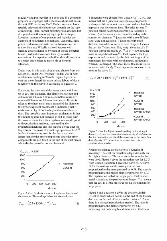
regularly and put together in a book and in a computer program to let people make economical estimations in the unit SEK excluding VAT. Each component has a specific price and the labour cost depends on the type of mounting. Here, normal mounting was assumed but it is possible with mounting high up, for example. Location, amount of components and logistics are example of parameters not included. Generally, these prices tend to overestimate due to discounts on the market but since Wikells is a well known well detailed cost estimator in Sweden, it should be better to use it without corrections than try to make corrections. An experienced builder should know how to correct these prices to match his or her real situation.

Ducts were in this study circular and chosen from the SR series, Lindab AB, Sweden (Lindab, 2004), with insulation according to Wikells. Figure 2 gives the cost per meter length for material and labour of ducts together with the curve fit according to Equation 2.

For ducts, the sheet metal thickness starts at 0.5 mm up to 250 mm diameter. The diameters 315 mm and 400 mm use 0.6 mm, 500 mm and 630 mm use 0.7 mm and 800 mm use 0.8 mm sheet metal. If care is taken to the sheet metal mass instead of the diameter, the power exponent becomes 0.8, indicating that it costs less per kg of duct to buy and mount a heavier duct. The probably most important explanation is that the mounting does not increase as fast as linear with the mass or diameter. Other explanations would point to the production methods, time used by the production machines and less logistic per kg duct for large ducts. The mass of a duct is proportional to d1.44.In fact, the mounting cost for the ducts are much larger than for the other components since the other components are just fitted in the end of the duct pieces while the duct must be cut and fastened.

(Cduct/lduct) / SEK

0

200

400

600

800

1000

1200

0 200 400 600 800

d / mm

Readings

Curve fit

Figure 2. Cost for ducts per meter length as a function of the diameter. The readings follow the standard sizes.

ductduct ldC 19.11300125 (2)

T-junctions were chosen from Lindab AB, TCPU, that means that the T-junction is a separate component. It is also possible to mount connectors on ducts but that approach was not chosen here. The price for one T-junction can be described according to Equation 3, where, dA is the main stream diameter and dB is the connection diameter. T-junctions with three different sizes were not available. T-junctions with three different sizes did not seem to exist. Figure 3 shows the cost for T-junctions. If dA = dB , the mass of a T-junction is proportional to dA

1.81. If dA = 400 mm, the mass is proportional to dB

2.64. That explains the high exponents and is caused by the fact that length of the component increases with the diameter, particularly when dB is changed. The sheet metal thickness is also increased with the dA. These exponents are close to theones in the curve fit.

. 49.291.1 199410908.90 BAT ddC (3)

CT / SEK

0

200

400

600

800

1000

1200

1400

0 200 400 600

d / mm

Readings

dA=dB

Curve fit

dA=dB

Readings

dA=dB·10 0̂.2

Curve fit

dA=dB·10 0̂.2

Figure 3. Cost for T-junctions depending on the straight diameter, dA, and the connected diameter, dB. dA = dB means that the connection duct is of the same size as the main flowduct. dA = dB·100.2 means that the connection is two standard sizes smaller.

Reductions change the size after a T-junction if necessary. The cost for reductions depended only on the higher diameter. The same curve form as for ducts were used. Figure 4 gives the reduction cost for RCU from Lindab. Equation 4 gives the curve fit. A curve fit for the cost against the mass gives the cost proportional to the mass powered by 0.88. The mass is proportional to the higher diameter powered by 2.02. The explanation is that for larger parts, thicker sheet metal is used and the part becomes longer. That meansthat the cost is a little bit lower per kg sheet metal for large parts.

Figure 5 and Equation 5 gives the cost for Lindab BU/BFU bends which occurs on the end of the branch duct and on the end of the main duct. At d = 315 mm there is a change in production method. The mass is proportional to the diameter powered by 2.12 indicating that both length and sheet metal thickness

215

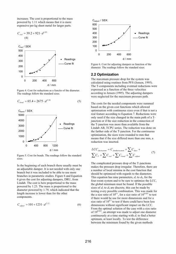
increases. The cost is proportional to the mass powered by 1.11 which means that it is more expensive per kg sheet metal for larger parts.

83.19212.39 dCred

(4)

Cred / SEK

0

100

200

300

400

500

0 200 400 600

d / mm

Readings

Curve fit

Figure 4. Cost for reductions as a functio of the diameter. The readings follow the standard sizes.

34.226754.65 dCbend (5)

Cbend / SEK

0

1000

2000

3000

4000

5000

0 400 800 1200

d / mm

Readings

Curve fit

Figure 5. Cost for bends. The readings follow the standard sizes.

In the beginning of each branch there usually must be an adjustable damper. It is not needed with only one branch but it was included to be able to use more branches in parametric studies. Figure 6 and Equation 6 gives the cost for adjusting dampers, DRU, from Lindab. The cost is here proportional to the mass powered by 1.23. The mass is proportional to the diameter powered by 1.79, which indicated that the length increase is lower than for the other components.

12.21231101 dCadjust (6)

Cadjust / SEK

0

100

200

300

400

500

600

0 200 400 600

d / mm

Readings

Curve fit

Figure 6. Cost for adjusting dampers as function of the diameter. The readings follow the standard sizes.

2.2 Optimization

The maximum pressure drop for the system was calculated using routines from PFS (Jensen, 1995). The T-components including eventual reductions were expressed as a function of the three velocities according to Jensen (1995). The adjusting dampers were neglected for the maximum pressure path.

The costs for the needed components were summed based on the given cost functions which allowed optimisation with continuous sizes even if that is not a real feature according to Equation 7. Reductions were only used if the size changed in the main path of a T-junction or if the size reduction in the connection of the T-junction was more than available from the Lindab AB, TCPU series. The reduction was done on the farther side of the T-junction. For the continuous optimisation, the sizes were rounded to mm that means that if the size differed more than one mm, a reduction was inserted.

adjustbendredT

ducttemfanductsysductsystem

CCCC

CCLCC (7)

The complicated pressure drop of the T-junctions makes the pressure drop irregular. Therefore, there are a number of local minima in the cost function that should be optimized with regards to the diameters. This equation has nine parameters, d1 to d9, for the four-room system and to be sure to optimize the LCC, the global minimum must be found. If the possible sizes of d1 to d9 are discrete, this can be made by testing every possible combination. This was made for the a size ratio of 100.1, for a size ratio of 100.025 to test if there would be use for more dimensions and for a size ratio of 100.2 to test if there could have been less dimensions without significant impact on the LCC. From the optimal solution of the case with a size ratio of 100.025, an attempt was made to adjust one diameter continuously at a time starting with d1 to find a better optimum, at least locally. To test the difference between the minimum found by the given methods

216

and the global minimum, a two-room case, according to Figure 7, was calculated with 1 mm step for the five diameters individually.

lb, d2 lb, d3

lc, d4 lc, d5lm, d1

Figure 7. The two-room case tested for a global minimum cost by use of 1 mm step for all d1 to d5.

For comparison, a fixed pressure drop per meter duct, R, for every duct section was tested as optimization method for the LCC. An optimal Ropt resulting in the lowest LCC was set for the whole system and compared to the case where all dimensions were independent.

A practical duct system must have all room connection ducts in the same size as the diffusers use. Here, 125 mm was assumed but for higher flows in office rooms, 160 mm is common. Otherwise, there must be a reduction between the branch and the room diffuser. There must also be enough distance between the reduction and the diffuser to get a developed flow profile before the diffuser. This is not a realistic solution. Therefore, all connection ducts must be 125 mm leaving only d1 to d5 in the example in Figure 1 to be varied. With all connection ducts set to 125 mm, the approaches can be repeated, namely all branch pieces independently set to the standard discrete sizes, or the best R can be found.

Finally, there are some reasons for not changing the duct size on a certain level of the duct system. In this example, it means that all the branch pieces will have the same size set with regards to the R for the first piece between the main duct and the first room. Even if Wiksell (2003) does not count for it, it will probably decrease the first cost because there is only one dimension through a certain corridor that must be handled. It will also decrease the static pressure and make the need for damping the nearest diffusers smaller. Flexibility regarding rebuilding and flow changes over time will also improve. A disadvantage is that the transport becomes more expensive since it would not be possible to place ducts inside each other.

2.3 Cost ratios

Assume that the cost can be expressed as Equation 8. The first term refers to the first cost, material and labour. If the cost for duct system is linear to the envelope area of the duct, m1 would be 1. The second term refers to the electrical energy cost. Equation 1 gives the electrical energy cost where d-m

2 is a part of pductmax. For a turbulent duct flow with constant friction coefficient, m2 is 5 (White, 1994).

21

21mm dadaC (8)

This cost should be derived with respect to the diameter and the derivative set to zero to find a minimum (se Equation 9). It can be shown that there is only one minimum m1 and m2 are positive.

0122

111

21 mm damdamdd

dC (9)

21

1

11

22mm

optam

amd (10)

Insertion of the optimal diameter (Equation 10) in the cost function (Equation 8) gives the cost at optimal diameter. Equation 11 gives the result.

21

2

21

1

11

222

11

221

mm

m

mm

m

opt

am

ama

am

amadC

(11)

Still, the first term expresses the first cost and the second term expresses the running costs. Equation 11 can be rewritten as Equation 12.

2

1

11

221 1

21

1

m

m

am

amadC

mm

m

opt (12)

This shows that the ratio between first cost and total cost do not depend on a1 or a2 and is expressed by

833.021

2

mm

m (13)

if m1 = 1 and m2 = 5.

If a simple duct is assumed, a2 includes the flow qtot

through pductmax but also the electricity price celectricity

and the length, lduct, if it is a duct. These parameters can be extracted from a2. a1 includes the length. For turbulent duct flow, the electrical power need is related to qtot

3. Equation 12 can be rewritten to Equation 14 where a1’ and a2’ are a1 and a2 divided with the extracted parameters respectively.

217

2

1

3

2

11

21

1'

''

21

1

21

1

21

1

m

mqcla

lam

mladC

mm

m

mm

m

yelectricitduct

mm

m

duct

ductopt

(14)

From Equation 14 it can be concluded that lduct

influences linearly on the optimal cost independent of m1 or m2.

2.4 Average flow versus discrete flow

The duct system is assumed to be designed for full occupancy, which means that qroom is present for all rooms. If the occupancy decreases below 1 and the system is a demand controlled system, the flow in each room depend on the system. For assembly halls it is reasonable to let the flow decrease for each room but for cell offices, the flow in a cell will be either low if the cell is not occupied or high if the cell is occupied in a binary pattern. For an ordinary demand controlled system with variable airflow rates, this is not of interest since the main pressure after the air handling unit is set and maintained by the air handling unit. For such a system, the pressure drop is constant for varying occupancy. There are also systems that decrease the main pressure when possible. The question is if it is reasonable to set the average flow for each cell instead of setting a high airflow rate for the occupied cells and a low for the vacant cells. By setting the average for all rooms, it is not necessary to know how many people there are in a room and which rooms are occupied and which are not resulting in a lower need for input data in simulations of such systems.

In this study, the pressure drop for a duct system was calculated for the case with the average airflow rate set for each room and for the case with design airflow rate set to a fraction of the rooms corresponding to the occupancy rates 25%, 50% and 75%. The other rooms were assumed to have zero airflow rates. In realistic cases, it is common to have a floor area dependent base airflow rate also for vacant rooms. By the chosen approach, the error should be smaller in a realistic case. Figure 8 shows the approach, where the number of rooms was a multiple of 4 and the occupied rooms were supposed to be spread out repetitively. The tested combinations are given by Figure 8 where 1 stands for 0.02 m³/s and 0 for zero airflow rate.

1 to 15 repetitions (4 to 60 rooms)

OR=50%

OR=50%

OR=75%

OR=75%

OR=25%

OR=25%

OR=25%

OR=25%

1 1 1 0

0 1 1 1

1 0 1 0

0 1 0 1

0 0 1 0

0 1 0 0

0 0 0 1

1 0 0 0

Figure 8. Different flow distributions compared to the average airflow rate set for all rooms. ‘1’ means 0.02 m³/s while ‘0’ means zero airflow rate. OR is the occupancy rate.

3. Result

Table 2. Optimal supply duct system for the two room example in Figure 7. The different costs and the resulting diameters are shown.

Co

ntin

ou

sly

Co

ntin

ou

sly

, o

ne

siz

e

at

a t

ime

Ra

tio

10

0.0

25

Ra

tio

10

0.0

5

Ra

tio

10

0.1

Ra

tio

10

0.2

Total 3581 3582 3586 3599 3625 3745

Electrical 318 324 334 285 230 592

Duct 3264 3258 3252 3314 3396 3153

T 114 114 114 116 118 111

Red 58 58 58 60 60 0

Bend 159 158 158 161 164 155

Adjust 115 115 114 116 116 110

pmax 22.0 22.5 23.1 19.8 15.9 41.0

d1 120 119 119 126 126 100

d2 120 119 119 126 126 100

d3 89 89 89 89 100 100

d4 85 86 84 89 100 100

d5 89 89 89 89 100 100

Costs / SEK

Maximum pressure drop / Pa

Dimensions of duct parts / mm

For the two-room case in Figure 7, calculations were made with the results given in Table 2. The default sizes were set according to Table 1 if nothing else is declared. Only a supply system was tested for different size steps of the components. The alternative when each diameter was varied continuously one at a time with the start solution as the optimal solution with the size ratio 100.025 compared to the alternative

218

with independently continuously set diameters show a small difference.

Table 3 gives the results for the four-room system in Figure 1 depending on the optimisation strategy. Table 3 gives the costs for different components as well as the optimal sizes for the different strategies of optimization. Both supply and exhaust systems are shown. The difference between supply and exhaust systems originates from the T-junctions that give different pressure drop for different directions. When the R-value is used for optimization, the span of the R-value, that gives lowest cost, is given. The set R-value

is the maximum allowed R-value. Due to the discrete sizes, the real R-value will be lower. At a certain level, there is a jump in dimensions. For one duct piece, the R-ratio between two adjacent sizes is approximately 100.1·5 = 3.16 since the pressure drop depends approximately on the inverse of the diameter powered by 5.

Table 4 shows the six best solutions for the supply system and their cost components and dimensions for the cases with all d1 to d9 as parameters and with d6 to d9 set to 125 mm respectively.

Table 3. Optimal duct system for the four room example given in Figure 1.

Ra

tio

10

0.0

25

Co

ntin

uo

usly

siz

es

fro

m f

orm

er

so

lutio

n

Ra

tio

10

0.1

Co

nn

ectio

n d

ucts

12

5 m

m,

ratio

10

0.1

Co

nn

ectio

n d

ucts

12

5 m

m,

Ropt

Co

nn

. 1

25

mm

, co

nst.

siz

e o

n le

ve

l, R

opt

Ra

tio

10

0.0

25

Co

ntin

uo

usly

siz

es

fro

m f

orm

er

so

lutio

n

Ra

tio

10

0.1

Co

nn

ectio

n d

ucts

12

5 m

m,

ratio

10

0.1

Co

nn

ectio

n d

ucts

12

5 m

m,

Ropt

Co

nn

. 1

25

mm

, co

nst.

siz

e o

n le

ve

l, R

opt

Total 7207 7201 7228 7494 7526 7625 7198 7192 7199 7516 7593 7673

Electrical 869 880 774 627 715 536 689 691 708 649 783 584

Duct 5603 5588 5648 6008 5896 6264 5729 5722 5712 6007 5894 6262

T 372 371 371 403 392 405 381 380 380 403 392 405

Red 68 67 131 130 191 71 70,8 70,7 70,8 130 191 71,4

Bend 173 172 179 179 180 204 179 179 179 179 180 204

Adjust 123 123 126 126 126 126 126 126 126 126 126 126

pmax 30.1 30.5 26.8 21.7 24.8 18.6 23.8 23.9 24.5 22.5 27.1 20.2

Ropt min 1.34 1.34 1.34 1.34

Ropt max 2.60 4.42 2.60 4.42

d1 149 149 160 160 160 160 160 160 160 160 160 160

d2 149 149 160 160 160 160 160 160 160 160 160 160

d3 149 149 160 160 160 160 160 160 160 160 160 160

d4 149 149 125 160 125 160 160 160 160 160 125 160

d5 94 94 100 100 100 160 100 100 100 100 100 160

d6 84 80 80 125 125 125 80 80 80 125 125 125

d7 84 83 80 125 125 125 80 80 80 125 125 125

d8 84 84 100 125 125 125 80 80 80 125 125 125

d9 94 94 100 125 125 125 100 100 100 125 125 125

Costs / SEK

Supply system Exhaust system

Maximum pressure drop / Pa

Duct pressure gradient at lowest LCC / (Pa/m)

Dimensions of duct parts / mm

219

Table 4. The six best solutions for a supply system. The best solution is the same as the one given in Table 3.

Ratio 100.1

Connections 125 mm, ratio 100.1

Total 7228 7260 7266 7267 7267 7275 7494 7520 7534 7564 7613 7614

Electrical 774 768 759 774 774 666 627 729 562 729 958 562

Duct 5648 5736 5695 5684 5684 5845 6030 5905 6125 6000 5780 6250

T 371 380 376 374 374 388 403 391 403 391 380 403

Red 131 70,8 131 131 131 70,8 130 190 131 131 190 70,8

Bend 179 179 179 179 179 179 179 179 187 187 179 202

Adjust 126 126 126 126 126 126 126 126 126 126 126 126

pmax 26.8 26.6 26.3 26.8 26.8 23.1 21.7 25.2 19.5 25.2 33.2 19.5

d1 160 160 160 160 160 160 160 160 160 160 160 160

d2 160 160 160 160 160 160 160 160 160 160 160 160

d3 160 160 160 160 160 160 160 160 160 160 125 160

d4 125 160 125 125 125 160 160 125 160 125 125 160

d5 100 100 100 100 100 100 100 100 125 125 100 160

d6 80 80 80 80 100 100 125 125 125 125 125 125

d7 80 80 80 100 80 100 125 125 125 125 125 125

d8 100 80 125 100 100 100 125 125 125 125 125 125

d9 100 100 100 100 100 100 125 125 125 125 125 125

Maximum pressure drop / Pa

Dimensions of duct parts / mm

Costs / SEK

A system with more than four rooms was not realistic to test for all sizes due to a huge amount of combinations possible. With the connection ducts to the diffusers fixed to 125 mm, up to twelve rooms were iterated. Figure 9 gives the LCC depending on approach and flow for up to twelve rooms, all with 125 mm connection size. The difference between supply and exhaust system is small for all situations.

LCCductsy stem / SEK

0

10000

20000

30000

40000

50000

0 2 4 6 8 10 12nroom

0.06 l/s, cons.

level Ropt

0.06 l/s, Ropt

0.06 l/s, size

ratio 10^0.1

0.02 l/s, size

ratio 10^0.2

0.02 l/s, cons.

level Ropt

0.02 l/s, Ropt

0.02 l/s, size

ratio 10^0.1

Figure 9. The LCC for a supply duct system similar to Figure 1 but with more rooms on the branch. Here, the approach with size ratio 100.2 is shown.

Figure 10 gives the increase in LCC for the one-branch supply system with all connection ducts set to 125 mm for different approaches of optimisation. At some points the difference is zero, which result in exactly the same dimensions.

Increase in LCC / %

0

1

2

3

4

5

2 4 6 8 10 12nroom

Size ratio

10^0.2

Optimal R

Optimal R,

constant

level size

Figure 10. The increase in LCC for a one-branch supply duct system with 125 mm connection ducts compared to the case with all sizes individually set with a size ratio of 100.1.

The case where R is varied to find an R resulting in lowest LCC for the duct system with twelve rooms is shown in Figure 11 where also the different components are presented. Each piece of the branch duct was given the maximum R-value. Figure 12 shows the same system with constant branch duct size set based on the first piece after the main duct. In Figure 12, it can be seen that when maximum Rincreases approximately 3.16 times, the duct is increased by one size. In Figure 11, there are more, smaller changes due to changes on parts of the branch.

220

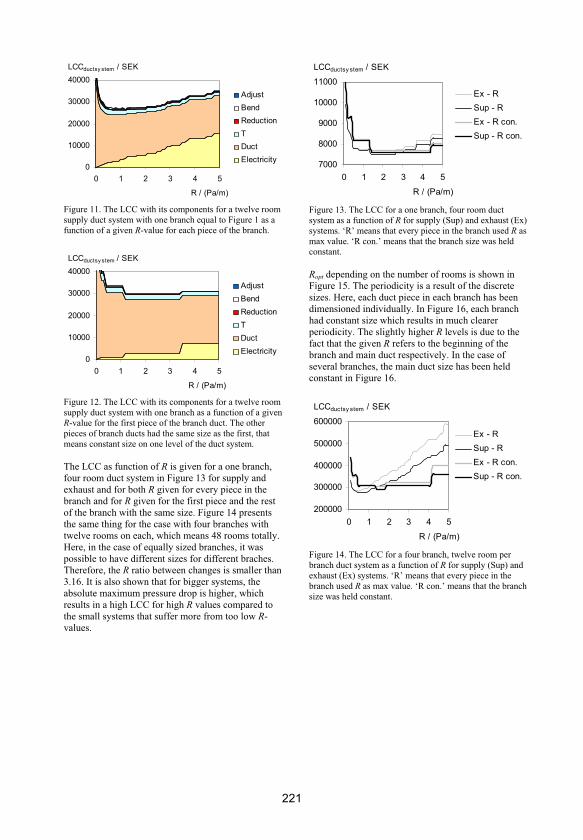
LCCductsy stem / SEK

0

10000

20000

30000

40000

0 1 2 3 4 5

R / (Pa/m)

Adjust

Bend

Reduction

T

Duct

Electricity

Figure 11. The LCC with its components for a twelve room supply duct system with one branch equal to Figure 1 as a function of a given R-value for each piece of the branch.

LCCductsy stem / SEK

0

10000

20000

30000

40000

0 1 2 3 4 5

R / (Pa/m)

Adjust

Bend

Reduction

T

Duct

Electricity

Figure 12. The LCC with its components for a twelve room supply duct system with one branch as a function of a given R-value for the first piece of the branch duct. The other pieces of branch ducts had the same size as the first, that means constant size on one level of the duct system.

The LCC as function of R is given for a one branch, four room duct system in Figure 13 for supply and exhaust and for both R given for every piece in the branch and for R given for the first piece and the rest of the branch with the same size. Figure 14 presents the same thing for the case with four branches with twelve rooms on each, which means 48 rooms totally. Here, in the case of equally sized branches, it was possible to have different sizes for different braches. Therefore, the R ratio between changes is smaller than 3.16. It is also shown that for bigger systems, the absolute maximum pressure drop is higher, which results in a high LCC for high R values compared to the small systems that suffer more from too low R-values.

LCCductsy stem / SEK

7000

8000

9000

10000

11000

0 1 2 3 4 5

R / (Pa/m)

Ex - R

Sup - R

Ex - R con.

Sup - R con.

Figure 13. The LCC for a one branch, four room duct system as a function of R for supply (Sup) and exhaust (Ex) systems. ‘R’ means that every piece in the branch used R as max value. ‘R con.’ means that the branch size was held constant.

Ropt depending on the number of rooms is shown in Figure 15. The periodicity is a result of the discrete sizes. Here, each duct piece in each branch has been dimensioned individually. In Figure 16, each branch had constant size which results in much clearer periodicity. The slightly higher R levels is due to the fact that the given R refers to the beginning of the branch and main duct respectively. In the case of several branches, the main duct size has been held constant in Figure 16.

LCCductsy stem / SEK

200000

300000

400000

500000

600000

0 1 2 3 4 5

R / (Pa/m)

Ex - R

Sup - R

Ex - R con.

Sup - R con.

Figure 14. The LCC for a four branch, twelve room per branch duct system as a function of R for supply (Sup) and exhaust (Ex) systems. ‘R’ means that every piece in the branch used R as max value. ‘R con.’ means that the branch size was held constant.

221

Ropt / (Pa/m)

0

1

2

3

0 5 10 15 20 25

nroom

1 branch

2 branches

3 branches

4 branches

5 branches

Figure 15. Optimal R when R was set for every duct piece in the branch and main ducts for a supply duct system. The connection ducts were 125 mm in diameter. If there was a span of R that gave the same LCC, the lowest R is shown.

Figure 17 shows the relative increase from the duct system based on Ropt for each duct piece individually and the case when the size has been constant for each branch and the main duct respectively. Figure 18 shows the maximum pressure drop corresponding to the situation in Figure 15. Figure 19 shows the maximum pressure drop corresponding to Figure 16. In Figure 19, the pressure drop is generally higher than in Figure 18 since the constant branch sizes tend to decrease the size in the beginning of a branch and increase the size in the end of a branch. The pressure drop depends on the square of the flow and the flow is highest in the beginning of a branch where the size is suppressed.

Ropt / (Pa/m)

0

1

2

3

0 5 10 15 20 25

nroom

1 branch

2 branches

3 branches

4 branches

5 branches

Figure 16. Optimal R when R was set for the first duct piece in the branch and main ducts respectively for a supply duct system. The connection ducts were 125 mm in diameter. If there was a span of R that gave the same LCC, the lowest Ris shown.

Relativ increase in LCC from optimal R to

optimal R with constant branch sizes

-0.02

0

0.02

0.04

0.06

0.08

0.1

0 5 10 15 20 25

nroom

1 branch

2 branches

3 branches

4 branches

5 branches

Figure 17. The relative increase from the duct system based on Ropt for each duct piece individually and the case when the size has been constant for each branch and the main duct respectively for a supply duct system

Max pressure drop at Ropt / Pa

0

20

40

60

80

100

0 5 10 15 20 25

nroom

1 branch

2 branches

3 branches

4 branches

5 branches

Figure 18. The maxium pressure drop in the case shown in Figure 16 with optimal R when R was set for every duct piece in the branch and main ducts. The connection ducts were 125 mm in diameter.

Max pressure drop at Ropt / Pa

0

20

40

60

80

100

0 5 10 15 20 25

nroom

1 branch

2 branches

3 branches

4 branches

5 branches

Figure 19. The maximum duct pressure drop in the case shown in Figure 17 with optimal R when R was set for the first duct piece in the branch and main ducts respectively for a supply duct system. The connection ducts were 125 mm in diameter.

Figure 20 gives the optimal LCC for the duct system depending on the number of rooms and number of branches. Here, the R has been set for each duct piece.

222

Due to the complicated expression of the pressure drops of the T-junctions, there is no simple correspondence between the number of rooms and the LCC. A curve fit for 1 branch gives LCC = 1654 + 888·nroom

1.35 and a curve fit for 12 rooms per branch gives LCC = 10521 + 20801·nbranch

1.15 in SEK. If the components on each connection cost more, this curve will be more linear. The optimal LCC as a function of number of branches have a more linear expression showing that there are more costs in the branch than in each room.

LCCductsy stem / SEK

0

100000

200000

300000

400000

0 5 10 15 20 25

nroom

5 branches

4 branches

3 branches

2 branches

1 branch

Figure 20. The LCC for the supply duct system as a function of number of rooms per branch and number of branches.

Figure 21 gives the influence from the energy price on the duct system optimal LCC. The first cost to LCC ratio is also shown. Since only small ducts are present in this twelve room, one branch case a new curve fit for ducts was made for the sizes between 80 and 200 mm, resulting in Cduct = 814·d0.59. Ducts make out most of the first cost according to Figure 9. Therefore it has been assumed that the first cost exponent in the cost function is 0.59. It is low because the chosen curve function but describes the cost on the form of the theoretical cost function given earlier. The pressure drop depends on the duct size powered by -4.85. Inserted in Equation 13, the resulting ratio between first cost and total cost becomes 89%. In the calculation, the ratio varies depending on the discrete diameters. If one branch and one room was calculated and the length of the duct pieces was increased to 30 m, 40 m and 20 m for the main duct, the branch duct and the connection duct respectively to suppress the influence from other components, the optimal discrete dimensions gave a ratio of 89%.

Equation 14 gives a correlation between the optimal LCC and the energy price to

21

1

mm

m

constLCC

With the same coefficients, m1 = 0.59 and m2 = 4.85, the theoretical exponent is 0.14. The curve fit

exponent based on the R set for every branch and main duct piece give the exponent 0.11.

LCCductsy stem / SEK Ratio / %

20000

25000

30000

35000

0 1 2 3 4

Energy price / (SEK/kWh)

70

80

90

100Ropt, con.

branch size,

LCC

Ropt, LCC

Ropt, ratio

Ropt, con.

branch size,

ratio

Figure 21. The duct system LCC for a one branch twelve room supply system as a function of the energy price for either R set to every duct piece or R set to the first piece in the branch and constant branch duct size. The ratio of the system that is made up of first cost is shown for the two cases. The connection duct sizes were 125 mm.

LCCductsy stem / SEK

0

25000

50000

75000

100000

0 20 40 60 80 100

qroom / (l/s)

8 m

6 m

4 m

2 m

Figure 22. The duct system optimal LCC for a one branch, twelve rooms supply duct system depending on the air flow rate for each room. The optimization method was to set maximum R for every duct piece in the branch and main duct. The connection ducts were 125 mm. The length between each room, was varied between 2 and 8 meter.

Figure 22 show the dependence of the flow on the duct system optimal LCC. According to Equation 14 and with m1 = 0.59 and m2 = 4.85, the LCC should be

33.021

13

mm

m

constLCC

A curve fit for 4 m between the rooms gave the exponent 0.32.

Comparisons were made to test if the average room airflow rate could be set to all rooms instead of using the correct airflow rates for each individual room if the occupancy gets below zero. Figure 23 presents the resulting pressure drop error according to the set-up in Figure 8.

223

Pressure drop error / Pa

-8

-6

-4

-2

0

2

4

6

0 20 40 60nroom

75%;1,0,0,0

50%;1,0

25%;1,0,0,0

25%;0,1,0,0

25%;0,0,1,0

25%;0,0,0,1

50%;0,1

75%;0,1,1,1

Figure 23. The maximum pressure drop for the average case minus the maximum pressure drop for the correct case for a one-branch supply duct system. The legend gives the occupancy rate followed by the room occupation sequence given by Figure 8.

4. Discussion and conclusions Different approaches to design duct system for ventilation purposes towards low life cycle cost was tested. The result shows that for a typical, practical duct system, the size of parts of a duct system is rather insensitive with regards to the life cycle cost. The cost increase from an idealized duct system to a practical system with constant sizes in each branch is 6% but increases a few percent units for larger systems.

A test of a number of different R-values and a choice of the one resulting in lowest life cycle cost give a sufficient optimisation for ordinary duct systems, both supply and exhaust. The R-value must be limited to avoid too high air speeds to avoid too much created noise. The acceptable speed is higher in larger ducts since they are located a longer distance from the rooms. By setting the R-value, the air speed will be lower in smaller ducts. Jagemar (1991) gives a maximum air speed of 3 m/s for connection ducts, a maximum air speed of 5 m/s for branch ducts and a maximum air speed of 8 m/s for main ducts. Themaximum speeds correspond to a maximum R of approximately 1.5 Pa/m. That, in fact, limits the life cycle cost optimization applicability.

There seems to be no need for more sizes. It could probably have been fewer but for practical reasons and velocity reasons, today’s sizes need to be preserved. In practice, a pressure loss per meter design around 1 to 1.5 Pa/m is used. This study, se Figure 11, confirms that these pressure gradients are reasonable and the LCC is not too sensitive for those practical Rvalues.

If the factors in Equation 1, like the energy price, change, Ropt will change. Equation 10 tells that the

optimal diameter is proportional to these factors powered by 1/(m1+m2). In the turbulent, constant friction case, Ropt is proportional to the optimal diameter powered by -5. That means that Ropt is proportional to, for example, celectricity powered by -5/6 = -0.833 if m1 = 1 and m2 = 5. A curve fit on the calculations give an exponent of -0.79. In conclusion, for example, if the life time of the system is clearly lower than 50 years, the maximum air speed will set the dimensions. On the other hand, if, for example, the electricity price will be much higher, an optimization regarding the issues in this study should be performed.

The cost modelling of components seem to be appropriate for estimating first costs. The theoretical cost functions seem to be appropriate if the actual components are described in the same way.

An average airflow rate for each room in a variable air volume situation simulation will give a small pressure drop error if the occupied rooms are repetitively spread. This error should be possible to neglect compared to the total pressure drop of a ventilation system. If the occupied rooms are not repetitively spread, for example if there are 40 rooms, and only the last 10 are occupied, this will imply an occupancy rate of 25% but the pressure drop error compared to the average approach would be much higher. This should be studied further on to test the benefit from airhandling unit main pressure control.

ReferencesASHRAE (1996), ASHRAE Handbook – HVAC Systems and Equipment, ASHRAE, Atlanta, United States

Besant, R.W., Aseidu, Y. (2000), Sizing and Balancing Air Duct Systems, ASHRAE Journal, v 42 (12), pp 24

Evans, R.A., Tsal, R.J. (1996), Basic tips for duct design, ASHRAE Journal, v 38 (7)

Jagemar, L. (1991), Energiekonomi – Val av fläktar och kanalutformning för luftbehandlingssystem i servicelokaler och industrier, Building Services, Chalmers, Gothenburg, Sweden, D10:1991, in Swedish

Jensen, L. (1995). Beräkningsuttryck för PFS, Dept. Of Building Services, Lund University, Lund, Sweden, Report TABK—95/7022, in Swedish

Jensen, L. (2000), Injustering av ventilationssystem – underlag för implementering, Building Services, Lund University, Lund, Sweden, TABK—00/7058, in Swedish

224

Johansson, D. (2002), Modelling LCC for different indoor climate systems, Licentiate thesis, Building Physics, Lund University, Lund, Sweden

Lindab (2004), Duct systems 2004-2007, Product catalogue, Lindab AB, Klippan, Sweden, http://www.lindab.com, 2005-08-02

Shitzer, A., Arkin, H., Study of economic and engineering parameters related to the cost of an optimal air supply duct system, ASHRAE Transactions, v 85 (2), pp 363-374

Tsal, R.J., Behls, H.F. (1990), Using the T-method for duct system design, ASHRAE Journal, v 32 (3)

White, F.M. (1994), Fluid Mechanics - third edition.,McGraw-Hill, Hightstown, United States

Wikells Byggberäkningar AB (2003), Sektionsfakta-VVS, Wikells byggberäkningar AB, Växjö, Sweden, in Swedish

Yeh, S.D., Wong, K-F.V. (1999), HVAC pipe/duct sizing using artificial networks, International Journal of Modelling and Simulation, v 19 (3), pp 282-286

225

226

Comparison between synthetic outdoor cli-

mate data and readings – applicability of Me-

teonorm in Sweden for building simulations

PAPER VI

Dennis Johansson Submitted to Theoretical and Applied Climatology 2005

227

228

Comparison between synthetic outdoor climate data and readings – applicability of Meteonorm in Sweden for building simulations

Dennis Johansson Building Physics Lund University LundSwedendennis.johansson@byggtek.lth.se

AbstractWhen building simulations regarding energy use and moisture design is performed, there is a need for outdoor climate data. In particular, this data include air temperature, vapour content or relative humidity, diffuse and direct short wave radiation, wind speed and wind direction. Today’s fast computers allow for calculations on a per hour basis which yields hourly data. For some simulations, the annual climate data should be normal and for some simulations, it should be extreme. A way to get all of this data is to use the computer program Meteonorm. It can simulate hourly climate data for normal and extreme years from all over the world. This paper compares data from the Meteonorm program with measured data from four Swedish locations 1991-2001. For outdoor temperature and degree hours for heating and cooling, the normal year of Meteonorm is a good approximation of the actual data even if the average measured temperature was higher for all locations than the normal Meteonorm temperature, probably due to the relatively warmer nineties. The difference between measured years is larger than the difference between Meteonorm and the measured average. The vapour content seems to differ more between Meteonorm and measurements but still Meteonorm should be appropriate to use. The short wave radiation is handled appropriately. The wind speed shows a systematic error for all locations which could be due to the measurement equipment.

1. Introduction

In the building industry, it is necessary to perform calculations regarding energy use and moisture levels in different parts of the construction. Due to demands such as the EU Directive on the Energy Performance of Buildings (Euroace, 2005), the need for calculations will probably increase. The mentioned calculations usually need data of the internal conditions and requirements that people desire from their building as well as outdoor climate data.

This paper focuses on the outdoor climate data. Since the computer capacity has increased, it is no problem to simulate buildings dynamically, which yields high resolution climate data to give any benefit. Usually, hourly data is used in dynamic programs (Strusoft, 2003; Equa, 2005). Hourly data resolves the day and night in sufficient number of steps, that are based on a wide spread unit. Even higher sampling rates could be used but the inertial behaviour of the heat capacity in

buildings and the inertial behaviour of the outdoor condition does not necessarily makes more data useful. Another reason for simulating on hourly basis is that meteorological stations usually store data with hourly resolution (SMHI, 2005).

Outdoor climate data are often available from the national meteorological institute in each country. A problem is that data are not available for every location. Due to the fact that the aim with these calculations, at least sometimes, is to give an average figure of, for example, the energy use, there is need for a normal year regarding the outdoor climate. Hourly data from a certain year is not reliable if average data is needed. The data must be normalized in that case. In other situation, extreme data is needed, for example to predict moisture damages in crawl spaces. A way to pass the problem of normal years would be to simulate over longer periods, for example 30 years, but that would yield a lot of data and we still do not know what next year would be like.

Examples of climate simulation models are given by Johansson (2002) for Swedish hourly temperature based on the annual average temperature and by Kalvova and Nemesova (1998) for daily extreme temperatures in Czech Republic. Mengelkamp (1999) tried to model wind speed and wind direction for Germany. Lefevre et al. (2002) discussed interpolation techniques and distances between weather stations.

To be able to compare the building calculations with actual measured result data for a specific year or period, the actual outdoor climate and indoor climate must have been measured and compared with the normal climate. In that case, a correction of, for example, the energy use must be done. This is discussed in literature for some parameters but not for many (Nilsson, 2003). Traditionally, only the outdoor temperature is corrected for but since the window area has increased over time and seems to be increasing, there is need for more sophisticated corrections (Bagge, 2005).

Meteonorm is a computer program that uses data from around 7400 weather stations all over the world to simulate synthetic hourly outdoor climate data for any location in the world (Meteotest, 2003). The program manual presents the theories behind the simulations. Table 1 shows the available parameters from the program. There are also a number of calculated parameters that can be obtained. The program can be specified to simulate average or ten-percentile extreme year regarding radiation and temperature. The used Meteonorm version was 5.0.1.

If the output data from Meteonorm are accurate enough, the program should make calculations for buildings easier when it comes to outdoor climate data

229

for different locations. There seems to be a lack of published comparisons between Meteonorm data and correct measured data. Müller (2001) discuss the use of Meteonorm as an applicable way to produce a normal year for the third world but there is a risk that it is not practically possible due to the cost of such software. Adsten et al. (2002) compared radiation simulations on solar collectors located in Lund, Stockholm and Luleå in Sweden both for the actual radiation data for the years 1983-1998 and for a Meteonorm normal year. They concluded that the Meteonorm based simulation was within the measured span of years for all locations but the average was not the same. Vogelsanger (2002) described a solar heating system test cycle. He states that Meteonorm data should preferably not be used since it over-estimates the fraction of diffuse radiation and since more time resolved data than hourly was needed.

Table 1. Parameters that can be written hourly by the Meteonorm program. The bold parameters were compared in this paper.

Global radiation horizontal Air temperature

Diffuse radiation horizontal Relative humidity

Beam Driving rain

Longwave radiation, incoming Precipitation

Longwave radiation, outgoing Cload cover fraction

Global radiation reflection

Radiation balance Wind speed

Extraterr. radiation Wind direction

UVA Global Air pressure

This paper compares outdoor climate data from Meteonorm with data from the Swedish Meteorological and Hydrological Institute, SMHI, for the period 1991-2001 for Lund and Frösön and 1991-1999 for Stockholm and Kiruna. The studied parameters were temperature, vapour content, global solar radiation, diffuse solar radiation, wind speed and wind direction. The result gives an idea of the applicability of the program and a magnitude for the error introduced with the program.

The main interest has been building simulations. The tested parameters were the ones available from measured data. The compared locations were also the ones measured on. The limited time span depended on the availability of measured data. That limitation made distribution comparisons unreliable. The Meteonorm data is mainly from the period 1960-1990 regarding temperatures, wind and vapour but from the last decade regarding radiation. If the outdoor climate has changed over time, this lead to an error. On the other hand, the normal year from the meteorological institutes are also from older periods and have the same disadvantage.

2. Methods

Measured data from SMHI was bought and analysed by a, for the purpose made, Delphi program. In the actual readings, there are sometimes data that are not relevant and wrong. A correction approach was applied in such a way that if a reading was clearly outside what the actual parameter possibly can be, the value from the hour before was used. The reason for this problem is probably when the measuring equipment fails. The Meteonorm data do not have any errors. They were saved from the program and analyzed in Excel. The compared locations are given by Table 2.

Table 2. The compared locations spread over Sweden. Location Latitude Longitude Altitude / m

Lund 55°43' N 13°13' E 73

Stockholm 59°21' N 18°04' E 30

Frösön 63°12' N 14°30' E 376

Kiruna 67°50' N 20°14' E 408

The studied parameters were recalculated in a way that they represent an interesting part in a building simulation. The studied parameters were also split into months, to be able to differ parts of the year. Weeks or days are not a realistic split due to the stochastic behaviour of the climate.

A common way to handle the outdoor temperature in buildings is by the use of degree hours. As long as the interior heat capacity is neglected and the heat transfer is assumed to be linear, the number of degree hours completely determines the transmitted heat through the building envelope. Therefore, degree hours were used for comparison together with average temperatures. The definition of degree hours is given by Equation 1 and 2. Dhheat is the number of degree hours for heating, Dhcool is the number of degree hours for cooling, tout,i is the outdoor temperature for hour iand tlm is the limit temperature, in this study set to 17°C. This is a reasonable balance temperature for a house with moderate insulation. Meteonorm assumed that a year has 8760 hours. In reality, there are leap years that increase the average number of hours per year slightly. That means that the measured data should have some more degree hours than the simulated data. The difference is small and was not corrected for. A monthly sum was also used as well as an average sum for each clock hour of the day. Accumulated outdoor temperature graphs were accomplished to give information about the extreme values of the entire measuring period and the Meteonorm normal year respectively.

8760

1, 0,max

iioutlmheat ttDh (°C·h) (1)

230

8760

1, 0,max

ilmioutcool ttDh (°C·h) (2)

Relative humidity was the measured and simulated parameter but the potential that drives the moisture through components is vapour content (Hagentoft, 2001). Therefore, month average vapour content was compared. Vapour content corresponds to the relative humidity through the saturation temperature. Curve fits based on tables in Nevander and Elmarsson (1994) are given by Equation 3 and 4, where t is the saturation temperature and v is the vapour content. For Equation 3, the correlation coefficient is 0.9999935 and the standard error is 0.0576. For Equation 4, the correlation coefficient is 0.999928 and the standard error is 0.250. These equations are valid between-30°C and 40°C.

5846

32

10577.110983.1

0001561.0009937.0

3460.0782.4

tt

tt

tv

(g/m³) (3)

2746.0

2746.0

446.6

6.2645.405

v

vt (°C) (4)

The solar radiations were integrated over time to give the incoming average power on a horizontal square meter over each month. That should represent the solar gain in the building. The global radiation is the total short wave incoming hourly average flux and the diffuse radiation is the incoming hourly average flux of short wave radiation when the sun is covered constantly. The direct radiation is the difference, which can be measured by a tube. SMHI measures the flux every 6 minutes for the direct radiation and the global radiation and integrate the hourly average.

The wind speed was compared as monthly average wind speed which corresponds to the volume of air that passes a square meter with its normal towards the wind. The wind influence on a building depends on the dynamic pressure, which depends on the wind speed squared. If the leaks in a building are of a turbulent nature, the pressure drop over a building component depends on the leakage flow squared. That means that the leakage flow depends linearly on the wind speed.

The wind direction is measured counter clockwise with 0 at north and refers to the direction from which the wind comes. The wind direction was not compared as average since the average value depends on the zero angle definition. With the chosen definition, if the wind direction is east half of the year and west half of the year, the annual average becomes south, which really does not give useful information.

Therefore, frequency curves are given for the wind directions. The frequency curve is the differentiated duration curve and shows the probability for a certain value of a parameter.

For the measured data, the average over the measured period was used for the month comparison but for the annual comparison, all measured years were presented.

3. Results

Climate parameters from readings were compared with Meteonorm both regarding normal and extreme years. In the graphs in this section ‘M h’ stands for the Meteonorm 10-percentile high extreme year, ‘M l’ stands for the Meteonorm 10-percentile low extreme year, ‘M’ stands for the Meteonorm normal year and ‘Av’ stands for the average of the SMHI readings for the measuring period. When the years are given in the graphs, only the two last digits are shown on the x-axis.

3.1 Outdoor temperature

The outdoor temperature was compared regarding annual average, total average, accumulated average annual outdoor temperature and number of degree hours for heating and cooling.

Average temperature

Figures 1-4 gives the average temperature for each measured year together with the temperatures from the Meteonorm normal and extreme years. The average from the measurements is also shown. Generally, the Meteonorm normal year gives lower average than the measurements. This effect becomes larger at southern locations. Since there are around ten measured years, one low extreme year and one high extreme year could be expected but the extreme years of Meteonorm seems to be further out in the distribution both on the low and high sides.

M h

M

M l

Av

Annual average temperature / °C

91 92 93 94 95 96 97 98 99 00 01

10

9

8

7

6

5

Figure 1. Annual average temperature for the readings for each year respectively together with the average from the extreme and normal years of Meteonorm for Lund.

231

M h

M

M l

Av

Annual average temperature / °C

91 92 93 94 95 96 97 98 99

10

9

8

7

6

5

4

3

Figure 2. The same as Figure 1 for Stockholm.

M h

M

M l

Av

Annual average temperature / °C

91 92 93 94 95 96 97 98 99 00 01

6

5

4

3

2

1

0

-1

Figure 3. The same as Figure 1 for Frösön.

M h

M

M l

Av

Annual average temperature / °C

91 92 93 94 95 96 97 98 99

2

1

0

-1

-2

-3

-4

Figure 4. The same as Figure 1 for Kiruna.

The monthly temperatures are shown in Table 3 where the measured temperatures are the average from the entire measuring period. The lower annual average temperature depends mostly on the winter part of the year.

Table 3. Monthly average temperatures for all locations in °C.

SMHI Met SMHI Met SMHI Met SMHI Met

Jan 0.9 -0.1 -1.2 -2.8 -5.4 -8.6 -10.9 -14.1

Feb 0.8 -0.7 -1.6 -3.5 -6.2 -7.5 -11.0 -12.3

Mar 2.7 2.2 1.3 0.0 -2.9 -3.4 -7.4 -8.3

Apr 6.9 5.5 5.0 4.5 1.1 1.0 -2.7 -2.1

May 11.7 11.2 10.4 10.7 6.5 7.2 3.0 3.9

Jun 14.4 14.2 14.6 15.2 10.5 11.6 9.5 10.2

Jul 17.7 16.8 18.4 17.4 13.8 13.4 12.6 13.0

Aug 17.7 16.1 17.5 16.8 12.8 12.5 10.5 10.9

Sep 13.0 12.6 11.9 12.1 8.2 7.9 4.9 5.0

Okt 9.3 8.4 6.9 7.4 3.0 3.8 -1.8 -1.9

Nov 4.3 4.3 2.2 2.7 -1.9 -2.2 -8.4 -8.3

Dec 1.5 1.1 -0.6 -0.9 -5.2 -6.0 -10.4 -11.4

Av 8.4 7.7 7.1 6.6 2.9 2.5 -1.0 -1.3

Lund Stockholm Frösön Kiruna

Accumulated temperature

Figure 5-8 gives the number of hours on the y-axis below a certain temperature on the x-axis. The left part of the Figures is a zoom-in on the low side of the middle part. The right part of the Figures is a zoom-in of the high side of the middle part. The general trend is that the curves corresponding to the measurements are more to the left than are the curves corresponding to the Meteonorm normal year. For all locations except Kiruna, it looks like the higher measured annual average temperature than simulated depends mostly on the extreme values since the curves are more to the left at the extreme values than in the middle part. For Kiruna, this effect is not clear. On the other hand, the difference between measured and simulated total average is small for Kiruna.

Annual hour

0

2000

4000

6000

8000

-10 0 10 20 30

Temperature / °C

SMHI

Met

Figure 5. Temperature duration curves for Lund. The SMHI values are the average of the entire measured period. ‘Met’ corresponds to the Meteonorm values for normal years.

232

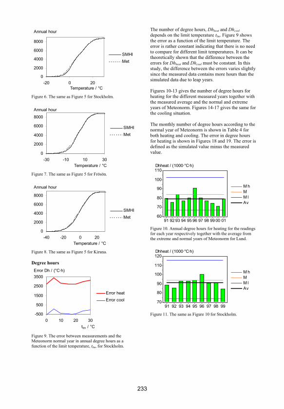
Annual hour

0

2000

4000

6000

8000

-20 0 20

Temperature / °C

SMHI

Met

Figure 6. The same as Figure 5 for Stockholm.

Annual hour

0

2000

4000

6000

8000

-30 -10 10 30

Temperature / °C

SMHI

Met

Figure 7. The same as Figure 5 for Frösön.

Annual hour

0

2000

4000

6000

8000

-40 -20 0 20

Temperature / °C

SMHI

Met

Figure 8. The same as Figure 5 for Kiruna.

Degree hours

Error Dh / (°C·h)

-500

500

1500

2500

3500

0 10 20 30

tlm / °C

Error heat

Error cool

Figure 9. The error between measurements and the Meteonorm normal year in annual degree hours as a function of the limit temperature, tlm, for Stockholm.

The number of degree hours, Dhheat and Dhcool

depends on the limit temperature tlm. Figure 9 shows the error as a function of the limit temperature. The error is rather constant indicating that there is no need to compare for different limit temperatures. It can be theoretically shown that the difference between the errors for Dhheat and Dhcool must be constant. In this study, the difference between the errors varies slightly since the measured data contains more hours than the simulated data due to leap years.

Figures 10-13 gives the number of degree hours for heating for the different measured years together with the measured average and the normal and extreme years of Meteonorm. Figures 14-17 gives the same for the cooling situation.

The monthly number of degree hours according to the normal year of Meteonorm is shown in Table 4 for both heating and cooling. The error in degree hours for heating is shown in Figures 18 and 19. The error is defined as the simulated value minus the measured value.

M h

M

M l

Av

Dhheat / (1000·°C·h)

91 92 93 94 95 96 97 98 99 00 01

110

100

90

80

70

60

Figure 10. Annual degree hours for heating for the readings for each year respectively together with the average from the extreme and normal years of Meteonorm for Lund.

M h

M

M l

Av

Dhheat / (1000·°C·h)

91 92 93 94 95 96 97 98 99

120

110

100

90

80

70

Figure 11. The same as Figure 10 for Stockholm.

233

M h

M

M l

Av

Dhheat / (1000·°C·h)

91 92 93 94 95 96 97 98 99 00 01

160

150

140

130

120

110

100

Figure 12. The same as Figure 10 for Frösön.

M h

M

M l

Av

Dhheat / (1000·°C·h)

91 92 93 94 95 96 97 98 99

190

180

170

160

150

140

130

Figure 13. The same as Figure 10 for Kiruna.

M h

M

M l

Av

Dhcool / (°C·h)

91 92 93 94 95 96 97 98 99 00 01

6 000

5 000

4 000

3 000

2 000

1 000

0

Figure 14. Annual degree hours for cooling for the readings for each year respectively together with the average from the extreme and normal years of Meteonorm for Lund.

M h

M

M l

Av

Dhcool / (°C·h)

91 92 93 94 95 96 97 98 99

7 000

6 000

5 000

4 000

3 000

2 000

1 000

0

Figure 15. The same as Figure 14 for Stockholm.

M h

M

M l

Av

Dhcool / (°C·h)

91 92 93 94 95 96 97 98 99 00 01

2 500

2 000

1 500

1 000

500

0

Figure 16. The same as Figure 14 for Frösön.

M h

M

M l

Av

Dhcool / (°C·h)

91 92 93 94 95 96 97 98 99

1 600

1 400

1 200

1 000

800

600

400

200

0

Figure 17. The same as Figure 14 for Kiruna.

Table 4. The number of annual degree hours for each month according to the normal year of Meteonorm.

Lund Stock-

holm

Frösön Kiruna Lund Stock-

holm

Frös-

ön

Kiru-

na

Jan 12696 14757 19042 23166 0 0 0 0

Feb 11891 13777 16486 19708 0 0 0 0

Mar 10990 12632 15177 18851 0 0 0 0

Apr 8253 8985 11517 13780 0.7 0 0 0

May 4376 4863 7322 9746 67 163 48 0

Jun 2439 1998 4009 5113 413 679 143 220

Jul 1371 1174 3031 3339 1221 1504 382 360

Aug 1584 1389 3605 4628 940 1214 222 111

Sep 3302 3655 6578 8636 167 155 6.9 0

Okt 6363 7150 9856 14091 0 0 0 0

Nov 9141 10267 13851 18234 0 0 0 0

Dec 11819 13337 17098 21130 0 0 0 0

Sum 84224 93983 127571 160421 2808 3714 801 691

Dhheat / (°C·h) Dhcool / (°C·h)

234

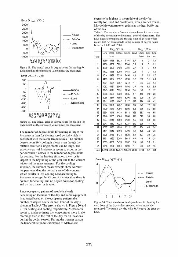
Error Dhheat / (°C·h)

-1000

-500

0

500

1000

1500

2000

2500

3000

Jan

Feb

Mar

Apr

May

Jun

Jul

Aug

Sep

Okt

Nov

Dec

Kiruna

Frösön

Lund

Stockholm

Figure 18. The annual error in degree hours for heating for each month as the simulated value minus the measured.

Error Dhcool / (°C·h)

-300

-250

-200

-150

-100

-50

0

50

100

Jan

Feb

Mar

Apr

May

Jun

Jul

Aug

Sep

Okt

Nov

Dec

Kiruna

Frösön

Lund

Stockholm

Figure 19. The annual error in degree hours for cooling for each month as the simulated value minus the measured.

The number of degree hours for heating is larger for Meteonorm than for the measured period which is consistent with the lower temperatures. The number degree hours for cooling is closer even though the relative error for a single month can be large. The extreme years of Meteonorm seems to occur in the period when it comes to the number of degree hours for cooling. For the heating situation, the error is largest in the beginning of the year due to the warmer winters of the measurements. For the cooling situation, the summer measurements show warmer temperatures than the normal year of Meteonorm which results in less cooling need according to Meteonorm except for Kiruna. At winter time there is no need for cooling, and no degree hours for cooling, and by that, the error is zero.

Since occupancy pattern of people is clearly depending on the hour of the day and some equipment is adjusted based on the occupancy pattern, the number of degree hours for each hour of the day is shown in Table 5. The error is shown in Figure 20 and 21 for heating and cooling respectively. Meteonorm seems to under-estimate the temperatures more in the mornings than in the rest of the day for all locations during the colder season. During the warmer season the temperature under-estimation of Meteonorm

seems to be highest in the middle of the day but mostly for Lund and Stockholm, which are sea towns. Maybe Meteonorm over-estimates the heat buffering of the sea.Table 5. The number of annual degree hours for each hour of the day according to the normal year of Meteonorm. The hour figure corresponds to the end time of an hour which means that ‘9’ corresponds to the number of degree hours between 08.00 and 09.00.

Hour

Lund Stock-

holm

Frösön Kiruna Lund Stock-

holm

Frös-

ön

Kiru-

na

1 3960 4455 5823 7191 5.7 18 0 1.3

2 4130 4639 5991 7308 3.1 14 0 1.1

3 4300 4824 6129 7401 2.7 11 0 1.2

4 4472 4918 6209 7451 2.5 11 0 1.5

5 4514 4938 6236 7456 4.1 15 0.4 1.7

6 4459 4854 6197 7396 5.7 23 1.0 2.8

7 4304 4684 6087 7272 11 36 3.6 4.4

8 4062 4431 5905 7092 25 59 6.1 6.6

9 3743 4111 5651 6830 54 95 12 12

10 3368 3689 5329 6535 97 145 23 20

11 3065 3374 4893 6296 153 209 39 30

12 2841 3137 4607 6127 217 276 56 42

13 2694 3008 4437 6030 272 329 72 50

14 2629 2976 4394 5998 308 366 85 59

15 2654 3046 4430 6018 326 383 93 65

16 2740 3135 4504 6068 321 379 94 68

17 2837 3245 4608 6139 289 350 88 66

18 2947 3362 4728 6227 240 295 77 62

19 3067 3483 4856 6322 183 234 60 54

20 3191 3612 4993 6423 128 176 44 43

21 3325 3756 5134 6528 82 127 29 35

22 3471 3922 5290 6643 45 83 15 28

23 3633 4100 5478 6767 23 50 5.1 21

24 3818 4285 5664 6903 11 30 0.4 16

Sum 84224 93983 127571 160421 2808 3714 801 691

Dhheat / (°C·h) Dhcool / (°C·h)

Error Dhheat / ((°C·h)/h)

-1

0

1

2

1 5 9 13 17 21

Kiruna

Frösön

Lund

Stockholm

Figure 20. The annual error in degree hours for heating for each hour of the day as the simulated value minus the measured. The sum is divided with 365 to give the error per hour.

235

Error Dhcool / ((°C·h)/h)

-0.3

-0.15

0

0.151 5 9

13

17

21

Kiruna

Frösön

Lund

Stockholm

Figure 21. The annual error in degree hours for cooling for each hour of the day as the simulated value minus the measured. The sum is divided with 365 to give the error per hour.

3.2 Vapour content

Figures 22-25 gives the vapour content for the different measured years together with the measured average and the normal and extreme years of Meteonorm.

M h

M

M l

Av

Annual average v / (g/m³)

91 92 93 94 95 96 97 98 99 00 01

9

8

7

6

Figure 22. Vapour content for the readings for each year respectively together with the average from the extreme and normal years of Meteonorm for Lund.

M h

M

M l

Av

Annual average v / (g/m³)

91 92 93 94 95 96 97 98 99

7

6

5

Figure 23. The same as Figure 22 for Stockholm.

M h

M

M l

Av

Annual average v / (g/m³)

91 92 93 94 95 96 97 98 99 00 01

6

5

4

Figure 24. The same as Figure 22 for Frösön.

M h

M

M l

Av

Annual average v / (g/m³)

91 92 93 94 95 96 97 98 99

5

4

3

Figure 25. The same as Figure 22 for Kiruna.

The monthly values of vapour content of a normal year of Meteonorm is shown in Table 6. The temperature influence is large. The two northern cities, that lie not at the sea, are dryer. Figure 26 show the monthly error in the vapour content.

Table 6. Monthly average vapour content according to the normal year of Meteonorm.

Lund Stock-

holm

Frös-

ön

Kiru-

na

Jan 4.3 3.5 2.4 1.6

Feb 4.0 3.3 2.7 1.8

Mar 4.6 3.8 3.4 2.4

Apr 5.4 4.8 4.5 3.4

May 7.1 6.2 6.3 5.0

Jun 9.1 8.5 8.4 6.8

Jul 10.5 10.1 9.4 8.6

Aug 10.4 10.2 9.2 8.2

Sep 9.0 8.3 7.3 6.1

Okt 7.2 6.7 5.7 3.9

Nov 5.8 5.1 3.8 2.5

Dec 4.7 4.0 2.9 2.0

236

Error v / (g/m³)

-1.5

0.0

1.5

3.0

Jan

Feb

Mar

Apr

May

Jun

Jul

Aug

Sep

Okt

Nov

Dec

Frösön

Kiruna

Stockholm

Lund

Figure 27. The error in vapour content for each month as the simulated value minus the measured.

3.3 Solar radiation

The diffuse radiation is not very much depending on the weather since it is present during the light part of the day anyway. The global radiation should depend more on the weather.

Global radiation

Figures 28-31 gives the annual global radiation for the different measured years together with the measured average and the normal and extreme years of Meteonorm.

M h

M

M l

Av

Average global radiation / (W/m²)

91 92 93 94 95 96 97 98 99 00 01

130

120

110

100

90

Figure 28. Global horizontal radiation for the readings for each year respectively together with the average from the extreme and normal years of Meteonorm for Lund.

M h

M

M l

Av

Average global radiation / (W/m²)

91 92 93 94 95 96 97 98 99

130

120

110

100

90

80

Figure 29. The same as Figure 28 for Stockholm.

M h

M

M l

Av

Average global radiation / (W/m²)

91 92 93 94 95 96 97 98 99 00 01

130

120

110

100

90

Figure 30. The same as Figure 28 for Frösön.

M h

M

M l

Av

Average global radiation / (W/m²)

91 92 93 94 95 96 97 98 99

100

90

80

70

Figure 31. The same as Figure 28 for Kiruna.

The extreme years of Meteonorm seems to correspond better to the distribution in the measurements than for temperature. Apparently, 1998 was not a sunny year. Table 7 gives the average global and diffuse monthly radiation. Figure 32 gives the monthly error where it can be seen that Meteonorm over-estimates the global radiation during summer.

Table 7. The monthly average horizontal radiation according to a normal year of Meteonorm in W/m².

Lund Stock-

holm

Frös-

ön

Kiru-

na

Lund Stock-

holm

Frös-

ön

Kiru-

na

Jan 19.0 13.9 10.9 0 12.9 10.1 6.8 0

Feb 40.9 40.0 38.6 19.9 24.8 24.7 18.8 12.4

Mar 77.0 90.7 79.8 59.7 50.9 46.3 40.6 31.4

Apr 160 151 151 136 76.0 82.4 73.3 66.8

May 207 220 214 184 109.1 111 97.7 91.3

Jun 216 246 247 206 95.1 106 111 105

Jul 225 217 236 182 110 105 103 95.2

Aug 176 174 166 137 92.9 95.0 81.9 78.4

Sep 111 107 87.8 68.5 64.6 61.1 53.5 43.9

Okt 57.9 50.9 42.9 25.4 35.8 31.0 26.0 16.3

Nov 29.8 19.0 13.0 4.4 18.5 13.6 8.6 3.4

Dec 13.8 10.0 4.0 0 9.8 7.6 3.5 0

Av 111 112 108 85.4 58.4 57.7 52.0 45.3

Global radiation Diffuse radiation

237

Error global radiation / (W/m²)

-30

-20

-10

0

10

20

30

40Jan

Feb

Mar

Apr

May

Jun

Jul

Aug

Sep

Okt

Nov

Dec

Frösön

Stockholm

Lund

Kiruna

Figure 32. The error in monthly average global radiation as the simulated value minus the measured.

Diffuse radiation

Figures 33-36 gives the annual diffuse radiation for the different measured years together with the measured average and the normal and extreme years of Meteonorm. The absolute variations between years is smaller than for the global radiation and it is not very dependent on the global radiation even if the diffuse radiation is included in the global radiation. Figure 37 gives the monthly error in diffuse radiation. The diffuse radiation is under-estimated by Meteonorm for Kiruna during summer probably due to an under-estimation of the diffuse radiation when there is midnight sun.

M h

M

M l

Av

Average diffuse radiation / (W/m²)

91 92 93 94 95 96 97 98 99 00 01

65

60

55

Figure 33. Diffuse horizontal radiation for the readings for each year respectively together with the average from the extreme and normal years of Meteonorm for Lund.

M h

M

M l

Av

Average diffuse radiation / (W/m²)

91 92 93 94 95 96 97 98 99

60

55

50

45

Figure 34. The same as Figure 33 for Stockholm.

M h

M

M l

Av

Average diffuse radiation / (W/m²)

91 92 93 94 95 96 97 98 99 00 01

65

60

55

50

Figure 35. The same as Figure 33 for Frösön.

M h

M

M l

Av

Average diffuse radiation / (W/m²)

91 92 93 94 95 96 97 98 99

65

60

55

50

45

Figure 36. The same as Figure 33 for Kiruna.

Error diffuse radiation / (W/m²)

-30

-20

-10

0

10

20

Jan

Feb

Mar

Apr

May

Jun

Jul

Aug

Sep

Okt

Nov

Dec

Stockholm

Lund

Frösön

Kiruna

Figure 37. The error in monthly average global radiation as the simulated value minus the measured.

3.4 Wind

The wind speed has the highest influence on building as long as they are not planned for a certain wind direction. The change in wind direction is not of that high frequency that it can be argued that the same air is moving back and forth.

238

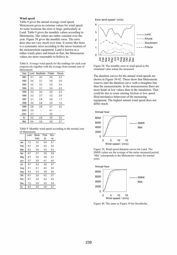
Wind speed

Table 8 gives the annual average wind speed. Meteonorm gives no extreme values for wind speed. At some locations the error is large, particularly at Lund. Table 9 gives the monthly values according to Meteonorm. The values are rather constant over the year. Figure 38 gives the monthly error. The error does also not vary much over time. It seems like there is a systematic error according to the micro location of the measurement equipment. Lund is known as a rather windy place and based on that, the Meteonorm values are more reasonable to believe in.

Table 8. Average wind speeds for the readings for each year respectively together with the average from normal year of Meteonorm.

Year Lund Stockholm Frösön Kiruna

1991 3.1 3.0 3.5 2.3

1992 3.0 3.1 3.6 2.5

1993 3.2 3.2 3.5 2.4

1994 3.3 3.1 3.4 2.2

1995 3.2 3.0 3.8 2.3

1996 3.3 2.7 3.3 2.9

1997 3.1 2.8 3.9 1.7

1998 3.0 2.8 3.5 1.2

1999 2.8 2.6 3.7 2.2

2000 3.5 - 4.1 -

2001 3.7 - 3.5 -

Av 3.2 2.9 3.6 2.2

Met 6.4 3.5 3.9 3.7

Table 9. Monthly wind speed according to the normal year of Meteonorm.

Lund Stock-

holm

Frös-

ön

Kiru-

na

Jan 7.2 3.5 4.0 3.7

Feb 6.7 3.6 4.0 3.5

Mar 6.2 3.6 4.0 4.2

Apr 6.7 3.7 3.5 3.8

May 6.7 3.6 3.8 3.7

Jun 5.7 3.5 4.1 4.0

Jul 5.7 3.2 3.8 3.7

Aug 5.1 3.1 4.0 3.6

Sep 6.2 3.3 3.8 3.6

Okt 6.7 3.6 4.2 3.7

Nov 6.7 3.5 4.2 3.5

Dec 7.2 3.5 3.5 3.4

Av 6.4 3.5 3.9 3.7

Error wind speed / (m/s)

0

1

2

3

4

Jan

Feb

Mar

Apr

May

Jun

Jul

Aug

Sep

Okt

Nov

Dec

Lund

Kiruna

Stockholm

Frösön

Figure 38. The monthly error in wind speed as the simulated value minus the measured.

The duration curves for the annual wind speeds are shown in Figure 39-42. These show that Meteonorm want to start the duration curve with a straighter line than the measurements. In the measurements there are more hours at low values than in the simulation. That could be due to some starting friction or low speed fluid mechanics behaviour of the measuring equipment. The highest annual wind speed does not differ much.

Annual hour

0

2000

4000

6000

8000

0 5 10 15

Wind speed / (m/s)

SMHI

Met

Figure 39. Wind speed duration curves for Lund. The SMHI values are the average of the entire measured period. ‘Met’ corresponds to the Meteonorm values for normal years.

Annual hour

0

2000

4000

6000

8000

0 5 10 15Wind speed / (m/s)

SMHI

Met

Figure 40. The same as Figure 39 for Stockholm.

239

Annual hour

0

2000

4000

6000

8000

0 5 10 15Wind speed / (m/s)

SMHI

Met

Figure 41. The same as Figure 39 for Frösön.

Annual hour

0

2000

4000

6000

8000

0 5 10 15Wind speed / (m/s)

SMHI

Met

Figure 42. The same as Figure 39 for Kiruna.

Wind direction

The wind direction frequency is shown in Figure 43-46 in polar graphs. ‘0’ angle corresponds to wind from north. All polar graphs are normalized to give the inside integral equal to 1 corresponding to all hours of the year.

0

0.0060

90

180

270

SMHI

Met

Figure 43. The wind directions for Lund according to measurements and Meteonorm. The angle unit is ° and the radial unit is h/° with 0.006 as maximum value.

0

0.0070

90

180

270

SMHI

Met

Figure 44. The same as Figure 43 for Stockholm.

0

0.0080

90

180

270

SMHI

Met

Figure 45. The same as Figure 43 for Frösön.

0

0.0080

90

180

270

SMHI

Met

Figure 46. The same as Figure 43 for Kiruna.

It looks like the wind directions of Meteonorm have errors but the trend is correct. On the other hand, the measuring equipment can be suspected to have errors to. The speed was also not combined with the direction to a wind velocity. At very low wind speeds, the direction instrument can probably keep its position until the wind speed increases.

4. Discussion and conclusions

To perform calculations regarding building physics, there is often a need for climate data. Meteonorm as a program to simulate hourly data was compared to measured data during the 1990s. The result tells the applicability of the climate simulation software.

Regarding temperature, vapour content and radiation, the Meteonorm normal year is within the spread of the actual years except vapour content and diffuse radiation for Kiruna. The measurement period is too short to give any significant information about extreme years but the extreme values of Meteonorm

240

seem to be more extreme than 10-percentile years for temperatures but for vapour content and radiation, it seems to be more correct. For wind speed and wind direction there is no extreme year simulation available.

Generally Meteonorm gives lower outdoor temperatures than the measurements show. The warmer reality than simulations during the 1990s can also be found by comparing with older measured data which indicates that the measured period was warmer than earlier in the 20th century. Particularly the winters were warmer which can be found by comparing the increase in temperature from the period 1960-1990 to the period 1991-2001. The average temperatures have increased more than the median temperatures indicating that the extreme values have increased most. That means that winters or summers have been warmer and this study indicates that mostly winters have been warmer.

The number of degree hours for heating follows the pattern of the outdoor temperature. The fact that the absolute error is almost constant as function of the limit temperature makes a degree hour correction possible without consideration to the limit temperature. The number of degree hours for cooling has large relative errors due to the relatively few absolute number of degree hours. The different measured years were highly spread due to the fact that the limit temperature is close to the summer temperatures which give a high relative spread. There seems to be a systematic error depending on the time of the day. This should be noticed and examined further for building simulations that need that information correctly.

The moisture content varies partly with the temperature. If the measured temperature was higher than simulated, it should be suspected that the measured vapour content was higher than simulated. In fact, the measured vapour content was remarkably lower than simulated for Frösön and Kiruna. From a moisture safety perspective, the use of Meteonorm should decrease the risks. Particularly during the summer period, the simulated data were over-estimated. For Lund and Stockholm, the error is smaller. A future study could look into the relative humidity in detail over a longer period to see if the particular measured years were exceptionally dry at Frösön and Kiruna.

The global radiation was over-estimated by Meteonorm for Frösön, particularly in the summer which is reasonable since the high absolute values belong to the summer. The diffuse radiation was under-estimated by Meteonorm for Frösön and Kiruna despite the statement by Vogelsang (2002).

For temperature, vapour and radiation purposes, Meteonorm seems to give plausible values regarding both averages and distribution. It is difficult to tell what a normal year is due to the short measured period, but the values of Meteonorm are reasonable for the location respectively. It is better to use Meteonorm for the wanted location than estimate with another location. There was also no evaluation of the correctness of the measured data. Error could be possible for single parameters due to the measuring equipment. The temperature duration curves show minor errors but the extreme values of the annual temperatures were appropriately modelled by Meteonorm for normal years and should be possible to use for power design.

For the wind speed, the error seems to be higher and systematic. For the wind direction, the error was also higher, but the wind direction should usually not influence a building simulation too much. An hypothesis to test in the future is that Meteonorm values should be used for wind speeds if the measurements are not taken from the exact location of the building. It also left to the future to test for co variation of two or more parameters.

In conclusion, based on this study, Meteonorm seems to be an appropriate program for generating climate data for building simulations when the aim is to make average predictions or risk assessments.

5. References

Adsten, M., Perers, B., Wäckelgard, E. (2002), The influence of climate and location on collector performance, Renewable Energy, 25, pp 499-509

Bagge, H. (2005), How passive solar heat affects energy use and indoor temperature, Submitted to 3rdInternational Building Physics Conference, 2006, Montreal, Canada

Equa (2005), IDA Indoor climate and energy 3.0,computer program, http://www.equa.se/, 2005-06-01

Euroace (2005), Energy Performance in Buildings Directive, http://www.euroace.org/bdirective.htm,2005-05-31

Hagentoft, C.E. (2001), Introduction to Building Physics, Studentlitteratur, Lund, Sweden

Johansson, D. (2002), Important factors of the LCC for indoor climate systems, Proceedings of the 6th Building Physics Symposium, Trondheim, Norway, Vol 2, pp889-896

Kalvova, J., Nemesova, I. (1998), Estimating Autocorrelation of Daily Extreme Temperatures in

241

Observed and Simulated Climates, Theoretical and Applied Climatology, 59, pp 151-164

Lefevre, M., Remun, J., Albuisson, M., Wald, L. (2002), Study on effective distances for interpolation schemes in meteorology, The XXVII Annual Assembly, European Geophysical Society, Nice, France

Mengelkamp, H.T. (1999), Wind Climate Simulation over Complex Terrain and Wind Turbine Energy Output Estimation, Theoretical and Applied Climatology, 63, pp 129-139

Meteotest (2003), Meteonorm handbook, manual and theoretical background, Switzerland, http://www.meteonorm.com/, 2005-06-01

Müller, E. (2001), Development of a test reference year on a limited data base for simulations on passive heating and cooling in Chile, Proceedings of the Seventh International IBPSA Conference, Rio de Janeiro, Brazil

Nevander, L.E., Elmarsson (1994), Fukthandbok – Praktik och teori, Svensk Byggtjänst, Stockholm, Sweden, in Swedish

Nilsson, A. (2003), Energianvändning i nybyggda flerbostadshus på Bo01-området i Malmö, Building Physics, Lund University, Lund, Sweden, TVBH-3045, in Swedish

SMHI (2005), Swedish Meteorological and Hydrological Institute, Norrköping, Sweden, http://www.smhi.se/, 2005-08-11

Strusoft (2003), VIP+, software manual, Limhamn, Sweden, http://www.strusoft.com (2005-02-04), in Swedish

Vogelsanger, P. (2002), The Concise Cycle Test Method – a Twelve Day System Test, IEA SHC Task 26, Subtask B, Solar Combisystems

6. Acknowledgements

A part of this work was carried out through course assignments made by Jimmy Nilsson and Håkan Ohlsson in their building physics education in Lund, Sweden.

242

Under-balancing mechanical supply and

exhaust ventilation systems with heat

recovery – effects on energy use

PAPER VII

Dennis Johansson Submitted to the Third International Building Physics Conference 2006, Montreal, Canada

243

244

1 INTRODUCTION

Since buildings are not completely air tight, wind and buoyancy will create unintentional air infiltra-tion, further on denoted leakage. Natural ventilation systems rely on these principles but they are not dis-cussed in this paper.

The leakage influences the energy use of the building. The heat recovery unit can not recover heat to air that enters the building through the construc-tion. If the mechanical ventilation system has lower supply airflow rate than exhaust airflow rate, further on denoted under-balanced, the rest of the supply air must be supplied through leaks in the construction. If the wind or buoyancy drives air into the building, this will not be a waste before air is exfiltrating the building due to wind or buoyancy. An under-balanced ventilation system means that there need to be a certain amount of natural forces before the infil-tration is unintentional.

That means that an under-balanced system de-creases the energy use for leakage but increases the

energy use for heating the supply air. On the other hand, the temperature efficiency of the heat recovery system increases based on the supply flow, when the supply airflow rate decreases. This paper compares these two effects due to under-balanced ventilation systems. If the supply airflow rate is zero, the system can be understood as a mechanical exhaust system only.

In cold climates, such as in Sweden, buildings should not have higher air pressure indoors than out-doors to avoid the indoor air, which has higher water content than the outdoor air, to be driven through the construction. If so, there is a risk for condensation since the wall, in a cold climate, gets colder and colder from inside to outside (Hagentoft, 2001).

The problem with moist air in the construction can be and is preferably reduced by a vapour barrier on the inside of the wall, which also reduces the en-ergy loss through unintentional infiltration even though complete air tightness is not realistic.

To further reduce the problem, the supply airflow rate of the ventilation system is usually designed to be slightly lower than the exhaust airflow rate, which means an under-balanced system. This design

Under-balancing mechanical supply and exhaust ventilation systems with heat recovery – effects on energy use

D. Johansson Building Physics, Lund University, Lund, Sweden

ABSTRACT: Mechanical supply and exhaust ventilation is usually slightly under-balanced. That means that the supply air flow rate is lower than the exhaust air flow rate. That is made in cold climates to prevent moist air from infiltrating the building construction parts. Usually, the exhaust air is more polluted so the exhaust filter pressure rises quicker than the supply filter pressure. The under-balanced ventilation therefore gives a margin to avoid over-pressure with time. If the ratio between supply and exhaust airflow rate is zero, the ven-tilation system can be understood as an exhaust only system. The under-balanced supply air flow affects the pressure difference between the inside and the outside of the house. This pressure difference in turn affects the sensitivity for infiltration due to buoyancy and wind. A higher under-pressure inside due to under-balance prevents air that comes in with the wind or buoyancy to pass through the building which means that the unin-tentional air leakage decreases. On the other hand, if the supply air flow is under-balanced, the available air flow for heat exchange in the heat recovery unit is decreased which means that the recovered heat decreases. This effect is dampened by the fact that the temperature efficiency related to the supply air of the heat recov-ery unit increases if the supply air flow is lowered. Still, the decreasing amount of recovered heat increases the need for heating the ventilation air. This study analyzed the effect of under-balanced supply air on the en-ergy use. Theories were compared to simulations with actual wind data for Swedish climate. It was found that there is a minimum energy use for an optimal under-balance ratio in some cases depending on the air tight-ness and the temperature efficiency of the heat recovery unit.

245

results in an under-pressure indoors, which means that the indoor air pressure is lower than the outdoor air pressure, preventing air to be driven through the walls. Since the exhaust filter gets polluted more rapidly than the supply filter, the under-balance also gives a margin against a decreasing exhaust airflow rate over time due to increasing filter pressure drop.

The mechanical ventilation is normally designed to handle requirements all the year round. Even if it would be possible to measure the air exchange rate inside the building and adjust the mechanical system to give the correct total airflow rate, including both ventilation airflow rate and leakage, this is not ap-plicable in practice since it is difficult to measure air exchange rates constantly.

Therefore, leakage is here seen as a waste that is not of use, even though it can be argued that, for ex-ample, research shows that people would work bet-ter with higher airflow rates, which occurs during windy days (Wargocki et al., 2000).

Thorsell (2005) showed by the use of the com-puter program VIP+ (Strusoft, 2003), that a ratio be-tween supply and exhaust airflow rate around 80% was an optimal under-balance ratio regarding heat-ing energy use. VIP+ is a building energy use calcu-lation program that takes into account pressure drops over single walls, wind and buoyancy. This study was made on a typical Swedish single family house. The typical under-balance ratio used by designers of air handling units is around 90%. The aim with this figure is to prevent from over-pressure indoors.

1.1 Objectives and limitation

The energy use for heating the air entering the build-ing either by the mechanical supply system with heat recovery or through the building envelope was ana-lyzed due to the under-balance of the supply airflow rate. Annually comparisons were performed with the intention to optimize the under-balance regarding the energy use and present the annual average leak-age.

A number of simplifications were made. Only the energy for air heating was taken into account. The energy use for fan electricity was not studied. Cool-ing was not studied. Only theoretical examples were calculated with no comparisons between calcula-tions and measured data.

2 METHODS

The positivistic methods used in this study were mainly model building based on theoretical princi-ples and simplifications. The hypothesis is that there, from an energy use perspective, is an optimal under-balance, which should be used in practice.

To make the necessary calculations, there is a need for describing the leakage depending on the

wind and buoyancy. The heat recovery unit must be described regarding the temperature efficiency as function of the supply air flow rate. The heating power for all entering air must be calculated and ap-plied with outdoor climate data to give examples of actual figures.

Table 1. The nomenclature used in this paper. * The unit varies with b.Quantity Description Unit Default

A1 Area, front wall m² 50

A2 Area, the other walls m² 150

A3 Area, roof m² 100

A4 Area, bottom floor m² 100

Am Envelope area m² 400

b Flow exponent - 0.7

Ci Flow factor, surface i *

cp Air heat capacity kJ/(kg·K) 1.0

fi Form factor -

h Height of building m 5.0

lf Specific leakage l/(s·m²) 0.8

Pinf Power for heating infiltration W

Psa Supply air heating power W

Pheat Total air heating power W

p0 Pressure inside Pa

pi Pressure on surface i Pa

pw Wind pressure Pa

pb Buoyancy pressure varation Pa

qex Exhaust airflow rate l/s 70

qexf Exfiltration l/s

qi Airflow rate into surface i l/s

qinf Infiltration l/s

qsa Supply airflow rate l/s 56

t Temperature difference °C 12

tex Exhaust temperature °C 22

thr Heat recovery temperature °C

tout Outdoor temperature °C 8

troom Room temperature °C 22

v Wind speed m/s 3.9

Wheat Total air heating energy Wh

y Height level in building m

Temperature efficiency

increase coefficient- 1.0

Temperature efficiency -

Reference temperature

efficiency- 0.70

Air density kg/m³ 1.2

2.1 Unintentional air infiltration

A house was used in this study as shown in Figure 1. This house is a one zone house that could contain two stories with a total floor area of 200 m². Based on Sandin (1990), the pressure obtained by the wind

246

outside each surface of the house can be described by Equation 1. The form factors, fi, were simplified to 0.7 for the front surface, with the wind direction as normal and -0.7 for the other sides. The bottom floor was supposed to have no influence from the wind. The nomenclature is given by Table 1.

qsa

10 m

p0 h = 5 m

10 m

p2, q2, A2

p4, q4, A4

qex

p3, q3, A3

v

p1, q1, A1

Figure 1. The example house used in the study. The air enter-ing through surface 2 refers also to the counter surface and the back surface since these three surfaces were assumed to have the same wind pressure coefficient, f2.

2

2v

ifpw (1)

Equation 2 gives the pressure variation obtained due to the buoyancy. This pressure variation is con-stant for the floor and the roof but varies with the height for the other walls where y can be referred to any height but p0 must be referred to the same height.

ytpb 04.0 (2)

To be able to describe each possible combination of buoyancy and wind influence, the building enve-lope was split into four parts. The indoor pressure is supposed to be p0. The pressure that drives air through the wall is the sum of the wind pressure and the buoyancy pressure minus the indoor pressure. The front wall is one part. The rest of the walls is one, the roof is one and the floor is one.

The airflow through an entire surface is given by Equation 3, but for the roof and the floor, no integra-tion is needed over the height. The constant b de-scribes if the flow is laminar, b = 1 or turbulent, b = 0.5, or somewhere between. Nevander and Elmars-son (1994) recommend 0.7 if there is no measure-ments, which was also used in this study as default. That means that the air flow rate is somewhere be-tween laminar and turbulent, which is reasonable due to the size of leaks. If b were 0.5 and the wind speed were doubled, that would result in a doubled airflow rate due to the wind. If b>0.5, an increasing

wind speed will increase the airflow rate through the wall more than linear.

hdy

bpytv

if

hi

Cqi

00

04.022

(3)

The walls can have incoming air below and out-going air above a certain height level at the same surface, which must be taken care of in Equation 3.

The constant Ci is given by Equation 4. Leakage in a house is measured as an airflow rate, lf at 50 Pa pressure difference per m² envelope surface (Boverket, 2002). The Swedish regulation gives the maximum value 0.8 l/(s·m²) for dwellings. All air going in through a wall, denoted infiltration, must be heated with the power Pinf. If air was going out from a wall, denoted exfiltration, it was assumed that it was unintentional leakage. The exfiltration is de-noted qexf. The infiltration is called qinf.

b

fl

iA

iC

50 (4)

Equation 5 gives flow continuity where constant density is assumed. The difference between all in-coming and all outgoing air is the air extracted by the exhaust fan minus the air supplied by the supply fan.

The difference between the mechanical exhaust airflow rate and the mechanical supply airflow rate must be equal to the sum of the airflow rates enter-ing the envelope by wind and buoyancy.

exfqq

saq

exqqqqq

inf4321 (5)

Equation 4 can be solved algebraically if b = 1 or if b = 1/2 and buoyancy is neglected but in realistic cases, a numerical solution for p0 is needed and thereafter a calculation of the airflow rates through each surface.

2.2 Heat recovery unit

The heat recovery unit recovers heat from the ex-haust air to the supply air. The temperature that the outdoor air can be heated to is described by Equa-tion 6. Freezing in the heat recovery unit was ne-glected.

outex

outhr

tt

tt (6)

The temperature efficiency of the heat recovery unit depends on the supply airflow rate. If the supply airflow rate decreases while the exhaust airflow rate is constant, increases, which is reasonable to be-lieve due to the longer time in the heat exchanger. It is not realistic that the temperature efficiency ex-

247

ceeds 1 but it is reasonable that it will be close to 1 at zero supply airflow rate.

In this study, it was assumed that the temperature efficiency followed Equation 7, with 0 taken from measurements of the heat recovery unit with equal airflow rates. Figure 2 shows the temperature effi-ciency used.

ex

sa

q

q11 00 10 (7)

0

1

010

·(1- 0)

qsa/qex

Figure 2. The temperature efficiency of the heat recovery unit based on the supply side as a function of the under-balance.

2.3 Power balance

Equation 8 gives the power needed to heat the infil-trating air to the room temperature.

outroomp ttqcP infinf (8)

The power needed to heat the air coming from the supply side of the heat exchanger to the room tem-perature is described by Equation 9. In this study, it was assumed that tex = 22°C and troom = 20°C. That means that it was assumed to be slightly warmer at roof level where the exhaust devices are located than in the centre of the room. The infiltrating air as well as the supply air is assumed to be heated to the room temperature. That means that the eventual internal heat gains were neglected.

hrroomsapsa ttqcP (9)

The two powers Pinf and Psa were summed to give the power needed to heat the total airflow rate, Pheat,for both ventilation and leakage. It was not analyzed how the air infiltration eventually influences for ex-ample the heat transmission. It was not analyzed how the electricity use for the fans changed even though it should benefit the under-balanced system since the pressure drop through the building is much lower than through the supply system.

To obtain the annual energy use, the wind speed and the outdoor temperature were inserted for each annual hour and the resulting powers were summed.

2.4 Outdoor climate data

Outdoor climate data was used regarding wind speeds and outdoor temperatures for the annual en-ergy use comparisons. These data were taken from Meteonorm (Meteotest, 2003) for average years for Malmö, southern Sweden, N55.6°, and Kiruna, northern Sweden, N67.8°. The annual average wind speed in Malmö is 5.5 m/s and the annual average outdoor temperature is 8.0°C. In Kiruna, the annual average wind speed is 3.7 m/s and the annual aver-age outdoor temperature is -1.2°C.

The wind measurements are usually made 10 m above the ground in free areas. This measured wind speed was scaled to 71% of the measured wind speed before it was used according to Sandin (1990). This was made since a typical house is located in a more crowded area with shading effects that lowers the air speed of the wind.

3 RESULTS

Results from the calculations are presented based on the typical house described. To determine the ratio between the supply and exhaust airflow rate from the difference between them, the actual exhaust air-flow rate is needed. The influence from leakage will be larger if the envelope area of the house is larger compared to the mechanical exhaust airflow rate.

Standard values for the different parameters were set according to Table 1. If nothing else is men-tioned, these values were used for the non-varied pa-rameters.

3.1 Unintentional air leakage

(qexf /Am)/(l/(s·m²))

0

0.1

0.2

0.3

0.4

0 50 100 150 200

(qex-qsa)/(l/s)

v=20 m/s

v=16 m/s

v=12 m/s

v=8 m/s

v=4 m/s

v=0

Figure 3. The leakage divided by the envelope area at differ-ent wind speeds. At a certain under-balance, the leakage is zero.

The air leakage, qexf, depends on all mentioned pa-rameters. The wind speed, v, and the outdoor tem-perature, tout, varies over time. The specific leakage,

248

lf, is a building design parameter. The areas and the height are probably determined by other aspects than the leakage and are constant. The form factors are determined by physics.

Figure 3 shows the leakage for the typical house at different differences between the exhaust and sup-ply airflow rate of the ventilation system.

Figure 4 shows the influence from the flow factor b and the specific leakage, lf. Here, t·h was 50°C·m and v was 3.9 m/s corresponding to the an-nual average wind speed of Malmö after topographic corrections.

(qexf /Am)/(l/(s·m²))

0

0.1

0.2

0.3

0 0.5 1 1.5 2

lf /(l/(s·m²))

b=0.5

b=0.7

b=1.0

Figure 4. The leakage depending on b and lf.

(qexf /Am)/(l/(s·m²))

0

0.2

0.4

0.6

0 5 10 15 20

v/(m/s)

h=40m

h=20m

h=10 m

h=0

Figure 5. The leakage as a function of the wind speed and the building height. At zero height, there is no influence from buoyancy.

The influence from different building heights is given by Figure 5. The default qex-qsa makes the leakage zero at low building heights. At high wind speeds, the height influence is negligible. Figure 6 gives the minimum air speed to obtain a leakage for different lf and qex-qsa.

v/(m/s)

0

5

10

15

20

0 20 40 60 80

(qex-qsa)/(l/s)

0.2

0.4

0.8

1.6

Figure 6. The minimum wind speed to get leakage at lf in l/(s·m²) shown in the legend. At highest lf, the buoyancy give a leakage up to qex-qsa = 30 l/s.

qexf /(Am·lf )

0

0.02

0.04

0.06

0.08

0.1

0 25 50 75 100

(qex-qsa)/(l/s)

1.6

0.8

0.4

0.2

Figure 7. The annual average leakage as a ratio of the leakage factor, lf, for Malmö.

qexf /(Am·lf )

0

0.02

0.04

0.06

0.08

0.1

0 25 50 75 100

(qex-qsa)/(l/s)

1.6

0.8

0.4

0.2

Figure 8. The annual average leakage as a ratio of the leakage factor, lf, for Kiruna.

The annual average leakage divided by Am and lf

is given by Figures 7 and 8 for the Malmö and Kiruna outdoor climate respectively. This means that if the lf = 0.8 l/(s·m²), the location is Malmö and

249

qex-qsa = 20 l/s, the annual average leakage is 4.4% of the measured value at 50 Pa.

3.2 Power need

The power need at a certain time with the parameters according to the default in Table 1 is shown in Fig-ure 9. The qex-qsa is rewritten to the ratio qsa/qex with qex at default value. There is a minimum that varies with lf. The linear behavior at low airflow rate ratios means that there is no leakage at all when qex-qsa in-creases.

Pheat/W

0

200

400

600

800

1000

1200

0 0.25 0.5 0.75 1

qsa/qex

1.6

0.8

0.4

0.2

Figure 9. The total power for heating the air at default condi-tions. The legend gives lf in l/(s·m²).

In Figure 10, the performance of the heat recov-ery unit is varied regarding 0 and . At those condi-tions, there is no optimum if the increase of the per-formance of the heat recovery unit is too small when qsa decreases.

Pheat/W

0

200

400

600

800

1000

0 0.25 0.5 0.75 1

qsa/qex

70%;0

70%;1

80%;1

Figure 10. The total power for heating the air at default condi-tions. The legend gives 0 and respectively.

3.3 Energy use

If the power at a certain condition is calculated for each annual hour, the annual energy use will be ob-tained. Figure 11 and 12 gives the annual energy use for heating all air for the Malmö case and the Kiruna case respectively.

Wheat/kWh

0

3000

6000

9000

12000

15000

0 0.25 0.5 0.75 1

qsa/qex

1.6

0.8

0.4

0.2

Figure 11. The annual energy use for heating air for Malmö depending on the ratio between supply and exhaust airflow rate. The legend shows lf in l/(s·m²).

Wheat/kWh

0

5000

10000

15000

20000

0 0.25 0.5 0.75 1

qsa/qex

1.6

0.8

0.4

0.2

Figure 12. The annual energy use for heating air for Kiruna depending on the ratio between supply and exhaust airflow rate. The legend shows lf in l/(s·m²).

The optimal ratio between the supply and exhaust airflow rate regarding the energy use for heating air depends slightly on the exhaust airflow rate, which is shown in Figure 13 for Malmö. Figure 14 gives qsa/qex at the lowest annual energy use for different

0 for Malmö. At a certain level around 0 = 80 %, the optimal ratio becomes one. For Kiruna, it was around the same value.

250

(qsa/qex)opt

0.8

0.85

0.9

0.95

1

0 50 100 150 200

qex/(l/s)

0.2

0.8

Figure 13. The optimal ratio between supply and exhaust air-flow rate due to an energy use perspective for Malmö. The fig-ures in the legend is lf in l/(s·m²).

(qsa/qex)opt

0

0.2

0.4

0.6

0.8

1

0 25 50 75 100

0/%

0.2

1.6

0.8

Figure 14. The optimal ratio between supply and exhaust air-flow rate due to an energy use perspective for Malmö. The fig-ures in the legend is lf in l/(s·m²).

4 DISCUSSION AND CONCLUSIONS

The leakage and the use of heating for the air de-pends on a number of parameters that has been nu-merically tested in this study. Generally, a low leak-age results in a low energy use for air heating. It is also shown that there is a minimum energy use at a certain under-balance in some cases, though there is no large influence on the energy use due to the un-der-balance that is needed for moisture safety in cold climates.

At certain cases, an optimal under-balance was shown to be lower than one. In a leaky house with a moderate heat recovery unit, the ratio between sup-ply and exhaust airflow rates can be typically 80% which is lower than the common design. For more air tight houses, the optimal ratio is higher.

On the other hand, the actual benefit from an op-timal design is lower with a more airtight house. In Malmö, an optimal design in the default case, with lf

= 0.8 l/(s·m²), can save 2.0% of the air heating en-

ergy or 120 kWh for the house compared to the bal-ances ventilation, which yields 6109 kWh annually. If it is assumed that the house has a floor area of 200 m², the energy use for air heating in the balanced case is 30.5 kWh/m² of floor which is reasonable.

If lf = 0.4 l/(s·m²) for Malmö with other parame-ters according to the default case, the energy use for balanced ventilation becomes 3923 kWh, or 19.6 kWh/m², and the saving from optimal under-balance would be 99 kWh which is 2.5%. That comparison clearly states that the air tightness itself is of much more importance for the energy use than the under-balance.

For the default case in Kiruna, the annual energy use is 9576 kWh, or 47.9 kWh/m², and the saving from optimal under-balance is 121 kWh or 1.3%. For the Malmö case, if 0 is lowered to 60% and the rest of the parameters are default, the saving due to optimal under-balance becomes 599 kWh or 8.4%.

The temperature efficiency of the heat recovery unit seems to highly influence the possible saving from under-balance. Here, it was assumed a linear increase when qsa decreased, but in further studies it should be measured how the heat recovery works with under-balance.

The computer program Enorm (Svensk Byggtjänst, 2000) is a common Swedish building energy calculation program that not calculates the wind pressure and wall pressure drops. In Enorm, it is assumed that there is a constant annual leakage of 5% of the measured value at 50 Pa pressure differ-ence, lf, for supply and exhaust systems. For exhaust systems, 4% is assumed.

The annual average leakage seems to be able to reach 10% of the leakage at testing pressure, 50 Pa. If an under-balance of 10%, or 7 l/s, and the Kiruna outdoor climate is used according to Figure 8, the figure becomes around 6%. An under-estimation of the annual average leakage result in an even higher under-estimation of the energy use since the leakage is higher at cold outdoor temperatures when the buoyancy is higher. This is shown in the data by comparison between the summed Pinf and a multipli-cation of the density, heat capacity, average flow and the number of degree hours. A b close to 1 would decrease the annual leakage to around 5% of the testing value.

If actual houses are protected locally by other buildings, fences or vegetation, the leakage should be lower than indicated in this study. On the other hand, the simplifications of the wind form factors, fi,to two average values for the whole building should increase the leakage since there are spots with higher negative form factors that can increase the leakage.

The ratio between the leakage for balanced venti-lation and for exhaust ventilation was 8 for the Malmö case, where the leakage is 8.8% for a system with 10% under-balance and 1.1% for a system with 100% under-balance. It can be argued that a house

251

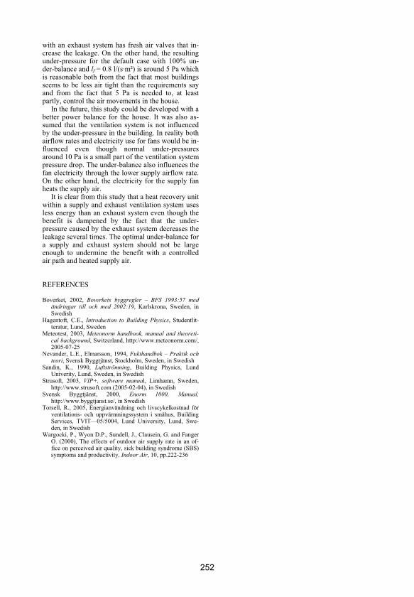
with an exhaust system has fresh air valves that in-crease the leakage. On the other hand, the resulting under-pressure for the default case with 100% un-der-balance and lf = 0.8 l/(s·m²) is around 5 Pa which is reasonable both from the fact that most buildings seems to be less air tight than the requirements say and from the fact that 5 Pa is needed to, at least partly, control the air movements in the house.

In the future, this study could be developed with a better power balance for the house. It was also as-sumed that the ventilation system is not influenced by the under-pressure in the building. In reality both airflow rates and electricity use for fans would be in-fluenced even though normal under-pressures around 10 Pa is a small part of the ventilation system pressure drop. The under-balance also influences the fan electricity through the lower supply airflow rate. On the other hand, the electricity for the supply fan heats the supply air.

It is clear from this study that a heat recovery unit within a supply and exhaust ventilation system uses less energy than an exhaust system even though the benefit is dampened by the fact that the under-pressure caused by the exhaust system decreases the leakage several times. The optimal under-balance for a supply and exhaust system should not be large enough to undermine the benefit with a controlled air path and heated supply air.

REFERENCES

Boverket, 2002, Boverkets byggregler – BFS 1993:57 med ändringar till och med 2002:19, Karlskrona, Sweden, in Swedish

Hagentoft, C.E., Introduction to Building Physics, Studentlit-teratur, Lund, Sweden

Meteotest, 2003, Meteonorm handbook, manual and theoreti-cal background, Switzerland, http://www.meteonorm.com/, 2005-07-25

Nevander, L.E., Elmarsson, 1994, Fukthandbok – Praktik och teori, Svensk Byggtjänst, Stockholm, Sweden, in Swedish

Sandin, K., 1990, Luftströmning, Building Physics, Lund Univerity, Lund, Sweden, in Swedish

Strusoft, 2003, VIP+, software manual, Limhamn, Sweden, http://www.strusoft.com (2005-02-04), in Swedish

Svensk Byggtjänst, 2000, Enorm 1000, Manual,http://www.byggtjanst.se/, in Swedish

Torsell, R., 2005, Energianvändning och livscykelkostnad för ventilations- och uppvärmningssystem i småhus, Building Services, TVIT—05/5004, Lund University, Lund, Swe-den, in Swedish

Wargocki, P., Wyon D.P., Sundell, J., Clausein, G. and Fanger O. (2000), The effects of outdoor air supply rate in an of-fice on perceived air quality, sick building syndrome (SBS) symptoms and productivity, Indoor Air, 10, pp.222-236

252

Dissertations from Building Physics, Lund University, Sweden

Bankvall C G Natural Convective Heat Transfer in Insulated Structures. Report 38. Heat Transfer in Insulation and Insulated Structure. Report 39.

1972

Sandberg P-I Moisture Balance in Building Elements Exposed to Natural Climatic Conditions. Report 43. (in Swedish)

1973

Bomberg M Moisture Flow through Porous Building Materials. Report 52. 1974

Samuelsson I Moisture Transfer in Steel Deck. Report 67. (in Swedish) 1976

Andersson A-C Internal Additional Insulation. Thermal Bridges, Moisture problems Movements and Durability. TVBH–1001. (in Swedish)

1979

Kronvall J Air Flows in Building Components. TVBH–1002. 1980

Jóhannesson G Active Heat Capacity. Models and Parameters for the Thermal Performance of Buildings. TVBH–1003.

1981

Hagentoft C-E Heat Loss to the Ground from a Building. Slab on the Ground and Cellar. TVBH–1004.

1988

Harderup L-E Concrete Slab on the Ground and Moisture Control. Verification of some Methods to Improve the Moisture Conditions in the Foundation. TVBH–1005.

1991

Bornehag C-G Mönsteranalys av inomhusluft – Undersökning av luftkvalitet i sjuka hus med flytspackelproblem. BFR Report no R23:1994. Swedish Council of Building Research. Stockholm. (in Swedish)

1994

Blomberg T Heat Conduction in Two and Three Dimensions. Computer Modelling of Building Physics Applications. TVBH–1008.

1996

Roots P Heat Transfer through a Well Insulated External Wooden Frame Wall. TVBH–1009.

1997

Arfvidsson J Moisture Transport in Porous Media. Modelling Based on Kirchhoff Potentials. TVBH–1010.

1998

Harderup E Methods to select corrections for moisture calculations at variable external climatic data. TVBH–1011 (in Swedish)

1998

Adalberth K Energy Use and Environmental Impact of New Residential Buildings. TVBH–1012.

2000

Engdahl F Air – for Health and Comfort. An Analysis of HVAC Systems’ Performance in Theory and Practice. TVBH-1013

2002

Johansson D Modelling Life Cycle Cost for Indoor Climate Systems. TVBH-1014 2005