Modelling, Imaging and Measurement of Distortion, Drag and ...

43rd AIAA Aerospace Sciences Meeting and Exhibit 10 – 13 January 2005, Reno, Nevada AIAA 2005-71

1 American Institute of Aeronautics and Astronautics Copyright © 2005 by the American Institute of Aeronautics and Astronautics, Inc. All rights reserved.

Modelling, Imaging and Measurement of Distortion, Drag and Break-up of Aircraft-icing Droplets.

Geoffrey Luxford, David W. Hammond and Paul Ivey

The School of Engineering, Cranfield University, Cranfield, Bedfordshire, MK43 0AL, UK

The distortion, drag and break-up of supercooled drizzle droplets in aircraft icing was in-vestigated in ambient conditions. An effective efficient computer procedure was developed for the distortion and drag of small droplets, < 1mm, at low Reynolds numbers, < 1000, and high Weber numbers, > 10. High-speed videos and photographs were obtained with an im-proved high-intensity LED strobe. Experimental measurements validated the drag model for droplets distorted by a rapidly accelerating airflow in a convergent wind tunnel. To prevent droplet coalescence, due to wake interactions, droplets were generated with a steady jet im-pinging of a rotating slotted disk.

Nomenclature CCD = Charge Coupled Detector SLD = Supercooled Large Droplets VeD = Volume Equivalent spherical Diameter VMD = Volume Mean spherical Diameter D = Droplet volume equivalent spherical diameter De = Droplet equator diameter U = Velocity of droplet, or velocity difference between air and droplet. a, g = Acceleration and gravity respectively a, b = Drop equator diameter and thickness respectively ρ, � = Fluid density and viscosity respectively σ = Surface tension a = Subscript for air d = Subscript for droplet Bo = Bond number for VeD = (ρd��a).g.D2/σ � ρd.g.D2/σ = ¾ We.Cd Cd = Drag coeff for droplet VeD. = F/(π.D2.ρa.U2/8) = 4/3.(ρd � ρa).a.D/ρa.U2 = 4/3.Bo/We Ci = Interpolated drag coefficient for equator = Csk .Cq(1-k) Cq = Disk drag coefficient, Cs = Sphere drag coefficient, F = Drag force on a droplet = a.(ρd � ρa).π.D3/6 = Cd.ρa.U2.π.D2/8 La = Laplace number = ρa.σ.D / �a

2 = Re2/We = 1/Oh2 (with gas properties) k = Drag interpolation factor = Log10(Ci/Cq) / Log10(Cs/Cq) Mo = Morton number = g.�a

4.(�d��a)/�a2.�3 � g.�a

4.�d/�a2.�3

= We2.Bo/Re4 Oh = Ohnesorge No. = �d/√(ρd.σ.D) Re = Droplet Reynolds number for VeD = ρa.U.D/�a, Rq = Reynolds number for equator diameter = ρa.U.De/�a, Td = Droplet oscillation period, = (π/4).√(ρd.D3/σ) We = Droplet Weber number for VeD = ρa.U2.D/σ, We2/Bo = Drag parameter for VeD = (�a.U4/g.�).(�a /�d) → 14.75 for free-fall droplets ρd/ρa = Density ratio Unless otherwise indicated the droplet dimensionless groups assume the VeD, or D, the velocity difference be-tween droplet and air, Abs(Ua � Ud), and the local air properties, ρa, �a.



I. Introduction As part of ongoing research into aircraft icing with supercooled drizzle droplets1, 100�m to 500�m, particular attention has been given to determining the distortion, drag properties and break-up of these droplets by meas-urement and imaging. This has been a substantial challenge because of the small size and high-speed of the drop-lets. For this droplets were generated and injected into an accelerating airflow in a convergent wind tunnel Another objective was to derive an improved model for the drag of small droplets distorted by strong aerody-namic forces. Experimental measurement were then required to determine the effect of droplet distortion on drag properties and verify the model.

II. Droplet Distortion and Drag Model The drag of oblate distorted water droplets can be much greater than for spherical particles of the same mass and volume because of the increased frontal area and also the more acute radius at the droplet equator. A requirement was to develop an efficient, effective, practical model of the distortion and drag of small droplets, < 500�m, at high Weber numbers, We > 10. A previous model of droplet drag characteristics1 determined a drag correction factor relative to that of a sphere at the same Reynolds number. While reasonable for many conditions, the model had a number of issues. 1. The reference sphere drag data of Maybank and Briosi2 had significant discrepancies with other data3. 2. The high-order curve fitting caused increasingly greater correction discrepancies for We > 12. 3. The model was not dependable for lower Reynolds numbers, Re < 1000. This resulted in a radical re-evaluation of how available drag and distortion data could be used to derive an effec-tive drag model for small water droplets in air at high Weber numbers and/or low Reynolds numbers. The full details of the model are beyond the scope of this paper and are presented elsewhere4. This depended on the drag properties determined from the terminal velocity of free-falling droplets in ambient air and stan-dard gravity. Such experiments2, 5, 6 provided data accu-rate to within one percent. The limitations of this data were that it was only avail-able for We < 10 and for a specific range of diameters and Reynolds numbers that were not appropriate for aircraft icing with freezing drizzle. The terminal free-fall velocity of water droplets tended to a maximum of just over 9m/s and also the parameter group We2/Bo, which is independent of droplet size, tended to an asymptotic limit of 14.75, as shown in Fig 1. The equation obtained for this are given in Ap-pendix 1. Equilibrium analysis of approximate models for highly oblate intact droplets showed that We2/Bo tends to a similar limit as We → �. At very low values, We < 2 x10-3, Re < 10, the droplets had slightly less drag than a rigid sphere, probably due to internal flow caused by the viscous drag. From this relationship, given in Appendix 1, it was pos-sible to calculate the drag for droplets of several mm diameter, since where the Weber number has a signifi-cant effect, We > 3, the Reynolds number only has a weak effect. For smaller water droplets, <1mm diame-ter, both the Weber number and Reynolds number can have a significant affect on the drag characteristics. For aircraft icing with freezing drizzle it is necessary to determine the distortion and drag of supercooled water droplets between 100�m and 500�m, where there can be a substantial effect from both Reynolds number and Weber number. It would appear that there is little directly relevant accurate data on the drag characteristics of such small droplets

Terminal conditions forfree-falling water droplets in air

0

10

20

30

40

0 5 10 15 20Weber number

We^

2 / B

o

Droplet, Maybank and BriosiDroplet, Scott, data from Gunn & KinzerDroplet, best fit extrapolation curveSphere, Clift, Grace & Weber data

Figure 1. Free-fall properties of droplets

Shape of sessile droplets on unwettable horizontal surface

0.0

1.0

2.0

3.0

4.0

5.0

6.0

7.0

8.0

-9 -8 -7 -6 -5 -4 -3 -2 -1 0 1 2 3 4 5 6 7 8 9r (mm)

y (m

m)

d=1.93, Bo=0.50, We=1.29 d=2.70, Bo=0.98, We=2.60d=3.48, Bo=1.63, We=4.10 d=5.81, Bo=4.55, We= 8.0d=7.91, Bo=8.44, We=11.10 d=12.06, Bo=19.6, We=17.0

Figure 2. Sessile droplet shape, numerical solution



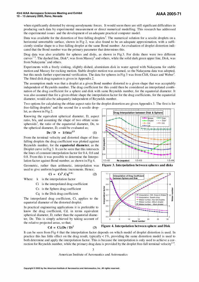
when significantly distorted by strong aerodynamic forces. It would seem there are still significant difficulties in producing such data by experimental measurement or direct numerical modelling. This research has addressed the experimental issues and the development of an adequate practical computer model. Data was available for the distortion of free-falling droplets3. The numerical solution for a sessile droplets on a horizontal unwettable surface, shown in Fig 2, was also found to be an adequate approximation, with a suffi-ciently similar shape to a free-falling droplet at the same Bond number. An evaluation of droplet distortion indi-cated that the Bond number was the primary parameter that determines this. Drag data was also available for spheres and disks, as shown in Fig 3. For disks there were two different curves7, 8. The dashed line, Disk*, was from Massey8 and others, while the solid dark green upper line, Disk, was from Nakayama7 and others. Experiments with a freely sinking, slightly dished, aluminium disk in water agreed with Nakayama for stable motion and Massey for rocking motion. Stable droplet motion was assumed, so the Nakayama data was adopted, but this needs further experimental verification. The data for spheres in Fig 3 was from Clift, Grace and Weber3. The fitted disk drag equation is given in Appendix 2. The assumption made was that a droplet at a given Bond number distorted to a given shape that was acceptably independent of Reynolds number. The drag coefficient for this could then be considered an interpolated combi-nation of the drag coefficient for a sphere and disk with same Reynolds number, for the equatorial diameter. It was also assumed that for a given oblate shape the interpolation factor for the drag coefficients, for the equatorial diameter, would also be adequately independent of Reynolds number. Two options for calculating the oblate aspect ratio for the droplet distortion are given Appendix 3. The first is for free-falling droplets3 and the second for a sessile drop-let, as shown in Fig 2. Knowing the equivalent spherical diameter, D, aspect ratio, b/a, and assuming the shape of two oblate semi-spheroids3, the ratio of the equatorial diameter, De, to the spherical diameter, D, could be evaluated as; De / D = 1/(b/a)1/3 (1) From the terminal velocity and distorted shape of free-falling droplets the drag coefficient was plotted against Reynolds number, for the equatorial diameter, as the Droplet curve in Fig 3. It can be seen that this intersects the lines of constant interpolation factor for 0.4, 0.6 and 0.8. From this it was possible to determine the Interpo-lation factor against Bond number, as shown in Fig 4. Geometric, rather than arithmetic, interpolation was used to give uniform logarithmic increments. Hence; Ci = Csk .Cq(1-k)

(2)

Where k is the interpolation factor Ci is the interpolated drag coefficient Cs is the Sphere drag coefficient Cq is the Disk drag coefficient. The interpolated drag coefficient, Ci, applies to the equatorial diameter of the distorted droplet. In practical engineering applications it is preferable to know the drag coefficient, Cd, in terms equivalent spherical diameter, D, rather than the equatorial diame-ter, De. This is simply achieved by taking account of the relative projected areas, so that; Cd = Ci.(De / D)2 (3) It can be seen from Fig 4 that the interpolation factor depends on which model of droplet distortion is used. In practice this has little effect on the drag result, typically < 1%, providing the same distortion model is used to both determine and apply the interpolation factor. This is because the interpolation is only used to achieve a cor-rection for Reynolds number, while the primary drag data is provided by the droplet free-fall terminal velocity2, 6.

1.0

0.4

2.0

1.E+02 1.E+03 1.E+04Re (equator)

Cd

(equ

ator

)

Drag Interpolation between Disk & Sphere

Sphere DiskDroplet Disk*0.4 0.60.8

Figure 3. Interpolation between spheres and disks

Interpolation of Drag Coefficientbetween Sphere and Disk

0.3

0.4

0.5

0.6

0.7

0.8

0.9

1.0

1.1

0 5 10 15 20 25 30Bond number

Inte

rpo

lati

on fa

ctor

0

5

10

15

20W

eber

num

ber

Interpolation, Clift, Grace & WeberInterpolation, Sessile dropWeber number, free-fall dropletsWeber number, 250um dropletWeber number, 50um droplet

Figure 4. Interpolation between sphere and Disk



To calculate droplet distortion it was first necessary to determine the Bond number from the Weber number. This can only be directly achieved for free-falling droplets, using the equations in Appendix 1. For other droplets sizes it is necessary to iteratively adjust the Bond number for equality with the Weber and Reynolds numbers. A rapidly converging iterative procedure for this is given in Appendix 6. For this iteration it was necessary to de-termine the interpolation factor, k, using the procedure given in Appendix 5. The resulting relationship between Bond number and Weber number is shown in Fig 4 for two sizes of droplet, 250�m and 50�m. It can be seen that at high Weber numbers the drag for the 250�m droplet is similar to the free-fall droplet, but the difference is more significant at lower Weber numbers. For 50�m droplets the Reynolds number correction had a more significant effect. The calculated and experimental results are compared in Fig 17.

III. Experimental Verification To experimentally validate the drag characteristics of distorted droplets it was necessary to be able to measure the Weber number, Reynolds number and Drag coefficient of the droplets. This required the ability to apply the necessary aerodynamic forces to the droplets and then record the resulting response. This was achieved by injecting droplets into an accelerating airflow in a small convergent wind tunnel1, shown in Fig 5. A critical part of this was to determine the aerodynamic force acting on the droplets, from which the drag coefficient could be determined. The force on a droplet in free-flight could not be directly measured, so the method used was to determine its ac-celeration. This required mono-dispersed droplets of calibrated mass to determine the drag force. To allow the necessary observations and measurements to be carried out three facilities were required;

1. Droplet generation and conditioning 2. Droplet visualisation 3. Measurement of droplet motion

IV. Droplet Generation & Conditioning The droplet generator was as explained in a previous report1, but this has since been streamlined for use inside the convergent wind tunnel of Fig 5. The transparent square convergent section of the tunnel was 520mm long. This had an electronically controlled suction fan, shown in the lower left inset of Fig 5. The generator produced a calibrated stream of mono dis-persed droplet, shown in the top row of Fig 6(a), how-ever the airflow along the droplet stream, needed to ap-ply the acceleration force, resulted in aerodynamic wake interactions which caused the droplets to clump together and coalesce, as shown in the 2nd and 3rd row of Fig 6(a). Figure 6(b) shows a high-speed video sequence at 50,000

pictures per second for the coalescence of two droplets of about 270�m diameter. This generation method resulted in both an excess num-ber and irregular size droplets, which significantly de-graded the measurement fidelity. To circumvent this an alternative method of generating the droplets was devel-oped. In this a continuous laminar jet was directed at a spinning slotted disc, shown left in Fig 7(a). This peri-odically allowed through a short length of the jet, shown right in Fig 7(a), which subsequently formed droplets.

Figure 5. Convergent Wind Tunnel

Figure 6. (a) Generated and coalescing droplets.

(b) Coalescence of a pair of 270�m droplets

Figure 7. (a) Spinning slotted disk drop generator

(b) Droplet from Spinning Slotted Disk



This resulted in a stream of droplet, with a VMD of about 250�m, as shown in Fig 7(b). It can be seen that these have the necessary spacing and spread, however the droplet size was quite variable. Since the method of determining the droplet acceleration did not allow simultaneously measurement of droplet size, the variability in the droplet size caused appreciable variability of the measured drag coefficient. This re-duced the fidelity of the measurements, although the average result was still of significant value. Improving the droplet generator to achieve suitable spacing of accurately calibrated mono-dispersed droplets is a primary tasks for future research.

V. Droplet Imaging The basic principles were considered in a previous pa-per1. In this the light from a pulsed LED (Light Emit-ting Diode) was focussed by a condenser lens onto the aperture of the imaging lens, as shown in Fig 8, to pro-vide bright field silhouette illumination of the droplets. While the method was able to produce droplet images, it lacked the necessary short flash duration, flash intensity and field of view.

A much improve LED strobe light was developed. This used high-power, high-frequency MOS-FET transistors to drive a high-intensity LED. This enabled a flash duration down to 50ns at 100kHz for high-speed video imaging. By using high-quality aspheric condenser lenses it was possible to achieve a field of view of up to 80mm diameter For single shot images it was possible to pulse the LEDs with 15A current for 50ns from a 60V source. The resulting very rapid change in current required careful circuit design and layout. For high-speed videos the pulse current was limited to 5A. The resulting flash unit shown on the left in Fig 12 mounted on the tripod. This had an externally triggered inter-nal adjustable pulse generator to control the flash duration. To test the speed of the flash light a length of fine wire was attached to the shaft of a motor and whirled around with a tip speed of 100m/s. The tip of this was then photographed with a single flash of various durations, from 50ns to 1�s. The results are shown in Fig 9. It can be seen that there was no noticeable motion blur for flashes of 200ns, or less. Figure 10 shows a typi-cal high-speed video image sequence of a droplet splash taken in the Cran-field vertical tunnel using the LED flash unit. The same illumination method was used for Figs 6(b) and 7. Figure 11 shows the droplet stream, surrounded by a cloud of fine spray, injected into to the wind tunnel, using the spinning slotted disc generator,

with the surplus water falling from the droplet generator. Figure 12 shows the high-speed video imaging arrangement. The LED strobe unit is on the left and Phantom V7 video camera is on the right. Figure 13 is a video sequence showing the distortion of a droplet of about 475�m as it approached a splash target at about 67m/s in the Cranfield vertical wind tunnel. Analysis of this gave a Weber number, perpendicular to the droplet, of about 28. The evaluated Bond number was about 51. The resulting droplet aspect ratio, 0.35, was bounded by the values 0.31 and 0.36 from the two distortion models. The evaluated drag coefficient, Cd, was about 2.4, for the VeD, or 5.5 times that of a sphere. It was noted that the droplet distortion was increasing as it approached the target.

Figure 8. Droplet imaging Optical Arrangement.

Figure 9. Speed test for LED flash light

Figure 10. Video sequence of splash for 400�m droplet

Figure 11. Wind tunnel droplet stream injection.



The arrangement for single shot images was similar to Fig 12, with a 6M pixel SLR digital camera and 105mm F2.8, 1:1 macro lens. A vertical laser beam across the tunnel, 5mm upstream of the imaging location, detected approaching droplets, with delayed triggering of the LED flash. The camera was manually trigger with 1/50th second exposure. The apparatus was covered with an opaque black velvet cloth to exclude most ambient light. Figure 14 shows different 250�m droplets at various

stages, from right to left, oblate distortion, bag formation and bag expansion. Figure 15(a) shows two images from a video sequence of the bursting bag for a 250�m droplet. Fig 15(b) shows the bag forming and bursting and Fig 15(c) a wide angle view of droplet break-up. At the time of writing these images were still being analysed and it was not possible to give spe-cific details about the conditions.

VI. Droplet Measurements A primary objective of the research was to experimentally determine the drag properties of distorted droplet in order to validate the droplet model. The method used, which was previously presented1, is shown in Fig 16. In this a droplet is detected by photo detectors as it intercepts three equispaced, parallel and coplanar laser beams. The droplet velocity and accel-eration were determined from the time intervals be-tween the resulting pulses from the photo detectors4. The full equations for determining the velocity and acceleration are given in Appendix 4. The rate of change of acceleration, or Jerk, can affect the measurements, but cannot be determined using the detector, which requires four laser beams. It is, how-ever, possible to evaluate the Jerk from other meas-urements, or from a simulation of the droplet motion. If the measurements were taken from video images, at equal time intervals, then ∆T1 = ∆T2 and � = 0. In practice the detector was constructed so the laser beams had equal spacing, hence ∆X1 = ∆X2 and α = 0.

Figure13. Pre-Splash Sequence

Figure 15. (a) Video sequence of bursting bag.

(b) : Video of bag formation and bursting

(c) : Break-up of droplet

Figure 14. Formation of bag instability.

Figure 12. Arrangement for High-speed videos

Figure 16. Droplet Measurement Method



It was inevitable that there would be some asymmetry in the spacing of the laser beams. Typically the minimum difference between the time intervals was about 10%. To achieve an acceleration accuracy of 2% with a beam spacing of 25mm required that the middle beam had to be within 25�m, or 0.01%, of the central position be-tween the two outer beams. The diode lasers were supported on adjustable screws at either end, so they could be accurately aligned on a calibration rig. This was a milling machining slide-way with digital readouts of 1�m resolution, which enabled the beams to be aligned within 10�m, To further eliminate any error due to unknown beam misalignment, the block holding the diode lasers could be inverted, so reversing any asymmetry errors. Hence averaging results from the normal and inverted orientations would cancel such errors.

VII. Predicted and Measured comparison of Droplet Drag Figure 17 shows results for 250�m water droplets from the droplet drag model and experimental measurements.

These are shown as the Bond number against Weber number, which represents the droplet drag force with re-spect to aerodynamic pressure. The drag coefficient for the VeD can be obtained from; Cd = 4/3 Bo / We (4) A difficulty with the experimental measurement was that of maintaining calibrated monodispersed droplets. As it was not possible to simultaneously measure the droplet size with the velocity and acceleration this resulted in appreciable experimental variability, as can be seen in Fig 17. Typically there was about 7% variance in the We-ber number and about 15% variance in the Bond number, as indicated by the error bars on the average values.

Measured acceleration characteristics of 250um droplets in convergent droplet tunnel, 40mm from exit and comparison with calculated results

1

10

100

1 10Weber number

Bon

dnu

mbe

r

Fan speed 2400rpm, Air velocity 136m/sFan speed 2100rpm, Air velocity 119m/sFan speed 1800rpm, Air velocity 102m/sFan speed 1500rpm, Air velocity 84m/sFan speed 1200rpm, Air velocity 67m/sAverage values250 micron distorted droplet250 micron spherical dropletFree-fall drops, in ambient air and gravityFree-falling spherical droplet

Figure 17. Predicted and Measured Results



The solid line in Fig 17 is the predicted characteristics for 250�m distorted water droplet, which is compared to the data for free-fall distorted droplets. It can be seen that at high Weber numbers, We > 10, hence higher Rey-nolds numbers, there is much less difference between the 250�m and free-fall droplets. Also shown are the pre-dicted results for spherical 250�m and free-fall droplets, which are clearly not related to the experimental results.

VIII. Conclusions 1. An efficient, effective procedure was developed for computing the distortion and drag of small liquid drop-

lets, 100�m < D < 1mm, in gas for low Reynolds numbers, Re < 1000, and high Weber numbers, We > 10. 2. Difficulties were encountered with maintaining mono-dispersed droplets for the experimental measure-

ments. With the vibrating nozzle generator the closely spaced droplets tended to coalesce in the accelerating airflow. The spinning slotted disk generator did not produce mono-dispersed droplets. This resulted in a variance of 15% to 20% in the experimental results.

3. The experimental results were sufficient to show the substantial effect of droplet distortion on the drag prop-erties and were consistent with the predictions made by the computational procedure for distorted droplets.

4. At a Weber number of 17 the drag predicted for distorted 250�m droplets was about four times that pre-dicted by the spherical droplet models.

5. The improved LED flash effectively enabled the required silhouette illumination of droplets for high-speed video and photographic imaging.

IX. Future Research 1. Develop a droplet generator to produce droplets of the required calibrated sizes and spacing. 2. Improved acceleration measurement to reduce need for precise alignment and to enable simultaneous meas-

urement of droplet size and shape. 3. Collect further data on droplet distortion, drag and break-up for a range of sizes and conditions. 4. Validate the computational procedure for droplet distortion and drag for a range of sizes and conditions. 5. Improve the LED flash light to allow frontal illumination of droplets and splashes. 6. Improve the imaging methods to obtain better resolution of the small, high-speed, droplets. 7. Develop various convergent wind tunnel profiles to investigate steady-state and transient droplet conditions. 8. Evaluate two dimensional droplet trajectories and lateral aerodynamic forces on distorted droplets

X. Appendix A. Appendix 1 Equations for Free-fall Water Droplets in Ambient Conditions, 20C @ 105Pa, with standard gravity, 9.81m/s2. For We > 5.3; Log10(14.75 – We2/Bo ) = 1.435 �� 0.1975 We or Bo = We2/(14.75 – 27.23 �� 10�� 0.1975 We) (5) For 0.25 <= We <= 5.3 and x = Log10(We) Log10(Cd) = 0.0985 x5 + 0.1901 x4 + 0.0382 x3 + 0.0616 x2 �� 0.1245 x �� 0.2682 where; Bo = ¾ We.Cd (6) For We < 0.25 the droplet behaves as a sphere3. This can be determined with the following iterative procedure for water and air at 20C @ 105Pa with g = 9.81m/s2 ; 1. Cd = 1.0 (initial estimate) 2. We = ρρρρa.U2.D/σσσσ: 3. Mo = g.��a

4.��d/��a2.��3

4. Bo = ¾.Cd.We 5. Re = (Bo.We2 / Mo)1/4 6. Cd = SphereDragCoeff(Re) Ref 3 7. Repeat from 4. until convergence (7)



B. Appendix 2 Equation for Drag Coefficient of a flat Circular Disk For Re < 39: Cq = SphereDragCoeff(Re) Ref 3 Otherwise, x = log10(Re): Cq = 10y, where; For 39 <= Re <= 283: y = ��0.61325 x5 + 5.0179 x4 �� 15.879 x3 + 24.401 x2 �� 18.503 x + 5.981 For 283 <= Re <= 3160: y = 0.1008 x5 �� 1.6452 x4 + 10.5463 x3 �� 33.009 x2 + 50.007 x �� 28.838 For Re > 3160 assume Re = 3160 (8)

C. Appendix 3 Equations for the Distortion Aspect Ratio of a Droplets; From Clift, Grace and Weber 3, For Bo < 0.4 b/a = 1 Else b/a = 1.0/(1.0 + 0.18 (Bo – 0.4)0.8) (9)

For a Sessile droplet, b/a = 1.0/(1.0 + 0.179 Bo0.821) (10) where a is the droplet equator diameter b is the droplet thickness. (b/a) is the droplet aspect ratio 3.

D. Appendix 4 Equation for calculating the Velocity and Acceleration from triple laser beam detector with constant Jerk.

U = (x/t).(1 + ��2.(1��2.��/ ��))/(1 �� 2) �� b.t2.(1 �� 2)/6 (11) a = (2.��.x/t2).(1 �� /��)/(1 �� 2) + 2.b.��.t/3 (12) Where; U is the droplet velocity at the central beam a is the droplet acceleration at the central beam b is the rate of change of acceleration, or Jerk

x1 = �X1 = X2 – X1 = x.(1 + �); x2 = �X2 = X3 – X2 = x.(1 – �) x = (x1 + x2)/2 � = (x1 – x2)/2.x t1 = �T1 = T2 – T1 = t.(1 + �); t2 = �T2 = T3 – T2 = t.(1 – �) t = (t1 + t2)/2 � = (t1 – t2)/2.t

E. Appendix 5 Calculation procedure for the drag interpolation factor for free-fall water droplet data at a given Weber number.

1. Determine Weber number for the droplet We = ρa.U2.D/σ (value from Appendix 6) 2. Obtain Morton number for ambient conditions Mo = g.�a

4.�d/�a2.�3, for 20C @ 105Pa, g = 9.81m/s2

3. Obtain free-fall Bo from We., Appendix 1 4. Determine drop distortion aspect ratio, (b/a) Appendix 3. 5. Evaluate equator diameter, De/D = (1 / (b/a))1/3.

6. Determine Reynolds number for VeD, Re = √(We√(Bo/Mo)) 7. Determine Equator Reynolds number, Rq = Re.(De/D) 8. Calculate drag coefficient of sphere for Rq, Cs = SphereDragCoeff(Rq) Ref 3. 9. Calculate drag coefficient of disk, Cq, for Rq Appendix 2 10. Determine Drag coefficient for droplet VeD Cd = 4/3.Bo/We 11. Correct drag coefficient for equator diameter. Ci = Cd.(D/De)2 12. Calculate droplet interpolation factor, k = Log(Ci/Cq) / Log(Cs/Cq)



F. Appendix 6 Calculation procedure for drag of a distorted droplet with a given size at a given Weber number.

1. Determine Weber number for given conditions We = ρa.U2.D/σ

2. Determine Laplace number for given conditions La = ρa.σ.D / �a2

3. Obtain droplet Reynolds number for VeD, Re = √(La.We) 4. Obtain initial estimate for Bo from We, Appendix 1. 5. Determine droplet distortion, (b/a), from Bo, Appendix 3. 6. Evaluate equator diameter, De/D = (1 / (b/a))1/3. 7. Obtain equator Reynolds number, Rq = Re.(De/D) 8. Obtain drag coefficient for a disk. Appendix 2 9. Obtain drag coefficient for a sphere. Cs = SphereDragCoeff(Rq) Ref 3 10. Calculate interpolation for drag coefficients. Appendix 5 11. Apply interpolation of drag coefficients, Ci = Csk .Cq(1-k)

12. Obtain drag coeff. for VeD, Cd = Ci.(De/D)2 13. Obtain revised Bond number, Bo = ¾.Cd.We 14. Repeat from 5 until convergence.

XI. Acknowledgements Thanks to Paul Spooner of the CAA for guidance, support and sponsorship of this research. Thanks to Tom Bond and Dean Miller at NASA for their help, advice, support and sponsorship of the LED flash unit and to Steve Markham for the circuit design, development and assembly. Thanks to Darchem Ltd for the stainless steel honeycomb flow straightener. Thanks to Stephen Cooke of Linx ink-jet printers for filter components. Thanks to EPSRC equipment loan pool for the high-speed video camera and Jolyon Cleaves of Photo-Sonics for help and advice on its use. Thanks to ADINA Research for provision of CFD/FEA facilities. Thanks to Dr Heather Al-mond for preparing the slotted disks. Thanks to Cranfield University, its staff and workshop for providing and constructing the necessary facilities. Thanks to Professor Freeman and others who helped with reviewing this paper. Thanks to everyone else who provided help, advice and support for this research.

XII. References 1. G. Luxford, D.W. Hammond, P. Ivey, “Role of Droplet Distortion and Break-up in Large Droplet Air-

craft Icing”. AIAA-2004-15411 2. J. Maybank & G.K. Briosi, 1961, “A Vertical Wind Tunnel”, Suffield Technical Paper No. 202, DRB

project no.D52-95-10-07. 3. R. Clift, J.R. Grace, M.E. Weber, 1978, “Bubbles, Drops & Particles”, Academic. 4. G. Luxford, 2005, PhD thesis on distortion, drag and break-up of small droplets. Due for submission to

Cranfield University in 2005. 5. W.J. Scott, Wood and Thurston, 1964, “Studies of Liquid Droplets Released from Aircraft into Vertical

and Horizontal Airstreams”. Data from reference 6. 6. R. Gunn and G.D. Kinzer, 1949, “The Terminal Velocity of Fall for Water Droplets in Stagnant Air” 7. Y. Nakayama & R.F. Boucher, 1999, “Introduction to Fluid Mechanics”, Arnold 8. B.S. Massey, 1989, “Mechanics of Fluids”, Chapman Hall, 6th Edition.



XIII. Addendum Addendum to AIAA05-0071; Modelling, Imaging and Measurement of Distortion, Drag and Break-up of Aircraft-icing Droplets; G. Luxford, D.W. Hammond and P. Ivey. In this paper the calculation procedure in Appendix 5, “Calculation procedure for the drag interpolation factor for free-fall water droplet data at a given Weber number”, was not as intended, although it was not necessarily incorrect. It was too late to amend the paper, so this Addendum was written and attached to clarify the issue. In calculating the drag of a distorted droplet, using interpolation between the drag of a sphere and disk, it is es-sential to clearly differentiate to which situation the parameters apply. In calculating the interpolation factor these have to be applied to the free-fall droplets. Confusion arose because the same Weber number was used for both the free-fall droplets and the small droplets being analysed to determine the interpolation factor using the procedure in Appendix 5. What was intended was that the same Bond number should be used in both cases. This is because it was found that the droplet distortion primarily depended on the Bond number, which was then used to determine the distortion, with one of the distortion models, from which the intermpolation factor was calculated using droplet free-fall data. At this stage of development there are issues and uncertainties about the best way to implement this interpolation method from available data. This will be resolved with better experi-mental data and more exact direct numerical simulation, which will also require experimental validation. A difficulty in computing Weber number from the Bond number is that the data for free-falling droplets, Appen-dix 1, determines Bond number from the Weber number. The inverse is, however, required, to obtain the Weber number from the Bond number. From the available formulation this requires an iterative procedure and the re-sulting Excel VBA macro procedure for this is given below, although some simplifications have been made.

G. Appendix 5 (Ammended) Private Function DragInterp(We, Bo, s%, c%, d%, o%) ' From an Excel VBA macro in Visual Basic ' Obtain interpolation factor between Sphere and Disk drag data using data for free-falling droplet data. ' We Weber number for droplet being analysed ' Bo Bond number for droplet being analysed ' s% selects drop shape option, 1 Clift, 2 Sessile drop ' c% selects disc drag option, either from Nakayama & Boucher7 (Appendix 2), or Massey8. ' d% selects sphere drag option, option 6 is from Clift, Grace and Weber3. ' o% output option selected (simplified to just the interpolation factor) Dim Wf, Bf, Mo, Ds, Dr, Re, Rq, Cs, Cq, Cd, Ci, kk, op If d% = 0 Then d% = 6 Else If d% <> 6 Then Stop Mo = MortonAmbient(293.1, 100000, 9.81) ' Morton number for ambient temp., pressure, gravity Wf = We: i = 0 ' Initial iteration conditions Do ' Start iteration loop Re = √(Wf .√(Bo / Mo)) ' Reynolds for sphere diam Bf = DropFall(Wf, 0, 2) ' Bond number for free-fall droplet (Appendix 1) Wf = √(Re4 .Mo / Bf) ' Weber number for free-fall droplet If Abs(Bo / Bf - 1) < 0.000001 Then Exit Do Else i = i + 1: If i > 99 Then Stop ‘ Iteration exit conditions Loop ' End of iteration loop Ds = DropShape(Bo, s%) ' Droplet aspect ratio, (Appendix 3)

Dr = (1 / Ds)1/3 ' ratio of Equator to Sphere diam Rq = Dr . Re ' Reynolds for equator diam Cs = SphereDragCoef(Rq, d%) ' Sphere drag coeff for RqRef 3

Cq = DiskDragCoef1(Rq, c%) ' Disk drag coef for RqRef 7, 8

Cd = 4/3 .Bo / Wf ' Drag coef for sphere diam Ci = Cd / Dr2 ' Drag coef for equator diam kk = Log10(Ci / Cq) / Log10(Cs / Cq) ' Log interpolatn factor. Select Case o% ‘ Select output option Case 1: op = kk ' output interpolation factor End Select DragInterp = op ' return results and exit funtion End Function This would be used in step 10 of of Appendix 6 and would replace the original version in Appendix 5.



The effect on the resulting calculation is shown in Figure 18. In this the disk drag data from Massey8 was used instead. This gave result very similar to the best fit to the average experimental result and to Figure 17 in the previous evaluation. For 250�m droplet the maximum difference in the result between using the Massey and Nakayama disk drag data was found to be about 5% at a Weber number of about 6.5. This amendment does not affect Figure 3 or 4, since these were computed by a different means which did not introduce the discrepancy.

This procedure results in a nested iteration and redundant computations, so is computationally inefficient. It should, however, be possible to modify the procedures of Appendix 5 & 6 so that only one iterative loop is re-quired, but there was not sufficient time and opportunity to develop this.

XIV. Addendum Conclusions 1. The revised procedure more correctly represented the intended interpolation method. 2. At present this is computationally less efficient, but could be revised to avoid the nested iteration. 3. With 250�m droplets and the Nakayama and Boucher7 disk drag data this gave poorer agreement with the

experimental results. Using the Massey8 data gave very good agreement with the best fit curve to the aver-age experimental results and was very similar to the results shown in Figure 17 for the previous procedure.

4. Further and better controlled experimental measurements are required to evaluate and validate the computer model and to determine the best combination and configuration using available data.

Measured acceleration characteristicsof 250um droplets in convergent droplet tunnel, 40mm from exit and comparison with calculated results

1

10

100

1 10 100Weber number

Bon

d nu

mbe

r

Fan speed 2400rpm, Air velocity 136m/sFan speed 2100rpm, Air velocity 119m/sFan speed 1800rpm, Air velocity 102m/sFan speed 1500rpm, Air velocity 84m/sFan speed 1200rpm, Air velocity 67m/sAverage values250 micron distorted droplet250 micron spherical dropletFree-fall drops, in ambient air and gravityFree-falling spherical dropletBest Fit, Average values

Figure 18. Experimental results in comparison with Model predictions, using Massey disk drag data

Modelling, Imaging and Measurement of Distortion, Drag and ...

Documents

Transcript of Modelling, Imaging and Measurement of Distortion, Drag and ...