Modelling galaxy close encounters by a parabolic problem

Introduction Dynamics of the parabolic problem Numerical results Conclusions

On the dynamics of the parabolic restricted threebody problem

E. Barrabes1 J.M. Cors 2 L. Garcia M. Olle2

1Universitat de Girona

2Universitat Politecnica de Catalunya

XV Jornadas de Trabajo en Mecanica Celeste

Barrabes, Cors, Olle (July 15, 2016) Parabolic problem 30/5/2016 1 / 28


Outline

Introduction

Dynamics of the parabolic problem

Numerical results

Conclusions



Galactic encounters: bridges and tails (I)

10

NGC 2535/6 NGC 7752/3

astromania.deyave.com/ www.etsu.edu/physics/bsmith/research/sg/arp.html www.spiral-galaxies.com/Galaxies-Pegasus.html

NGC 3808

Bridges!




9

Tails!

Arp 173

• NGC 2992/3

http://www.astrooptik.com/Bildergalerie/PolluxGallery/NGC2623.htm www.etsu.edu/physics/bsmith/research/sg/arp.html

http://www.ess.sunysb.edu/fwalter/SMARTS/findingcharts.html

NGC 2623




Galaxies NGC 3808A (right) and NGC 3808B (left). Credits: NASA, HubbleSpace Telescope (2015)



Galactic encounters: bridges and tails (II)

Toomre, A. and Toomre, J. Galactic bridges and tails, The AstrophysicalJournal, 178, 1972.



Galactic encounters: bridges and tails (II)Toomre, A. and Toomre, J. Galactic bridges and tails, The AstrophysicalJournal, 178, 1972.



Motivations and Aims

Close approach of two galaxies: it cause significant modification of themass distribution or disc structure. One particle that initially stays in onegalaxy (or around one star), after the close encounter, it can jump to theother galaxy or escape.

To study the mechanisms that explain that a particle remains or notaround each galaxy, considering a very simple model: the planarparabolic restricted three-body problem.



Outline

Introduction


Numerical results

Conclusions



The Planar Parabolic Restricted Three-Body Problem



Equations (I)

Parabolic problem:

d2Z

dt2= −(1− µ)

Z− Z1

|Z− Z1|3− µ Z− Z2

|Z− Z2|3,

Z2 = −Z1 = 12 (σ2 − 1, 2σ), and σ = tan(f/2)

Change to a synodic frame (primaries at fixed positions) + change of time:

z1 = (−1

2, 0), z2 = (

1

2, 0),

dt

ds=√

2 r3/2.

Compatification to extend the flow when the primaries are at infinity(t, s→ ±∞):

sin(θ) = tanh(s).



Equations (II)

Global system

θ′ = cos θ,z′ = w,w′ = −A(θ)w +∇Ω(z)

where ′ =d

dsand

A(θ) =

(sin θ 4 cos θ−4 cos θ sin θ

),

Ω(z) = x2 + y2 + 21− µ√

(x− µ)2 + y2+ 2

µ√(x− µ+ 1)2 + y2

.



Upper and Lower boundary problems

Global system Boundary problems θ′ = cos θ,z′ = w,w′ = −A(θ)w +∇Ω(z)

−→θ=±π/2

z′ = w,w′ = ∓w +∇Ω(z)

dim 5 dim 4



Main properties (I)

Equilibrium points at the boundaries (as in the RTBP):

Collinear: L±i = (xi, 0, 0, 0,±π/2), i = 1, 2, 3

Triangular: L±i = (µ− 12 , yi, 0, 0,±π/2), i = 4, 5

Stability:

L+1,2,3 L+

4,5

dim(Wu) 1 2dim(W s) 4 3

L−1,2,3 L−4,5dim(Wu) 4 3dim(W s) 1 2



Main properties (II)

Jacobi function: semi gradient property (no periodic orbits)

C = 2Ω(z)− |w|2, dC

ds= 2 sin θ|w|2

Hill’s regions: 2Ω(z)− C ≥ 0 → C-criterium

−π/2 −→ θ −→ 0

-2

-1

0

1

2

-2 -1 0 1 2

y

x

-2

-1

0

1

2

-2 -1 0 1 2

y

x

-2

-1

0

1

2

-2 -1 0 1 2

y

x

π/2 ←− θ ←− 0



Main properties (III)

Homothetic solutions and connections

θ = π/2

θ = −π/2

θ = 0

L+1

L+4

L+3

L−3L−

4

L−1



Dynamics of the problem

In order to describe the dynamics of the parabolic problem, we will focus ontwo aspects:

the final evolutions in the synodical system when time tends to infinity,

the richness in the intermediate stages due to

existence of invariant manifolds associated with the homothetic solutions

heteroclinic connections that allow the existence of orbits with passagesclose to collinear and/or equilateral configurations.



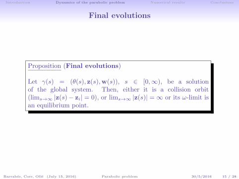
Final evolutions

Proposition (Final evolutions)

Let γ(s) = (θ(s), z(s),w(s)), s ∈ [0,∞), be a solutionof the global system. Then, either it is a collision orbit(lims→∞ |z(s)− zi| = 0), or lims→∞ |z(s)| =∞ or its ω-limit isan equilibrium point.



Connections in the the upper boundary problem

m1 m2∞

m1 ∞ m2

L+4

L+5

L+1 L+

3

L+2



Outline

Introduction


Numerical results

Conclusions



Explorations

Role of the invariant manifolds in the sets of connecting orbits betweenprimaries

Equal masses (µ = 0.5):Barrabes, Cors, Olle Dynamics of the parabolic restricted three-bodyproblem Communications in Nonlinear Science and Numerical Simulation,29: 400–415, 2015

Different masses (µ < 0.5):Work in progress with L. Garcıa and M. Olle



Connecting orbits with passages to collinear or triangularconfigurations

Connection of type mi − Lk −mj :

collision orbit with mi backwards in time

collision orbit with mj forwards in time

along its trajectory it has a close passage to Lk



Connecting orbits: examples (µ = 0.5)

-1

-0.5

0

0.5

-0.5 0 0.5 1

y

x

m2 − L3 − L2 −m2/m1



Connecting orbits: examples (µ = 0.5)

-4

-2

0

2

4

-4 -2 0 2 4

m1

m0

m2

-3000

-1500

0

1500

3000

-3e+06 -1.5e+06 0 1.5e+06 3e+06

Y

X

m1

m2

m0

-30

-15

0

15

30

-200 -100 0 100 200

m1

m2

m0



Symmetric connecting orbits (µ = 0.5)

Connection mi −mi: crosses the section θ = 0 such that y = x′ = 0

I.C. (x0, 0, 0, y′0)

Connection mi −mj : crosses the section θ = 0 such that x = y′ = 0

I.C. (0, y0, x′0, 0)




mi −mi

-6

-4

-2

0

2

4

6

-4 -3 -2 -1 0 1 2 3 4

y’

x

-0.4

-0.3

-0.2

-0.1

0

0.1

0.2

0.3

0.4

0.3 0.4 0.5 0.6 0.7 0.8 0.9 1 1.1

-4

-3

-2

-1

0

1

2

3

4

-8 -6 -4 -2 0 2 4 6 8




mi −mj

-10

-8

-6

-4

-2

0

2

0 1 2 3 4 5

x’

y

capture m2capture m1C=C(L3)

-0.3

-0.25

-0.2

-0.15

-0.1

-0.05

0

0.05

0.1

0.15

0.2

-0.8 -0.6 -0.4 -0.2 0 0.2 0.4 0.6 0.8

-4

-3

-2

-1

0

1

2

3

4

-8 -6 -4 -2 0 2 4 6 8




The invariant manifolds of L±i , i = 1, 2, 3 separate the regions of capture

-3.33108

-3.33103

-3.33098

-3.33093

0.52952 0.5296 0.52968

x’

y

a

c-b

d-e

f

-2

-1

0

1

-2 -1 0 1 2

y

x

ab

cd e f




The hetero/homoclinic connections of L±i , i = 1, 2, 3 separate the regions ofcapture

L−3 → L+

3

L−1 → L+

1

L−2 → L+

2

L−3 → L+

1

L−1 → L+

3

L−2 → L+

2



Bridges and Tails?

We consider a bunch of initial conditions around m1 for θ = −π/4. We take asnapshot of each particle at certain θ > 0 and classify them depending theirfinal evolution:

-4

-3

-2

-1

0

1

2

3

4

-4 -3 -2 -1 0 1 2 3 4

Y

X

Capture m1 Capture m2



Bridges and Tails?

We consider a bunch of initial conditions around m1 for θ = −π/4. We take asnapshot of each particle at certain θ > 0 and classify them depending theirfinal evolution:

-4

-2

0

2

4

-4 -2 0 2 4

Y

Y

Capture m1 Escape



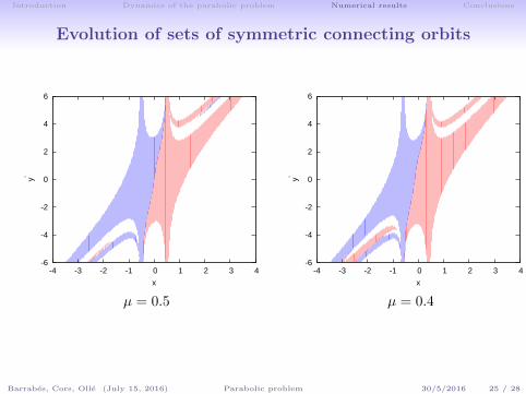
Evolution of sets of symmetric connecting orbits

-6

-4

-2

0

2

4

6

-4 -3 -2 -1 0 1 2 3 4

y’

x

-6

-4

-2

0

2

4

6

-4 -3 -2 -1 0 1 2 3 4

y’x

µ = 0.5 µ = 0.4




-6

-4

-2

0

2

4

6

-4 -3 -2 -1 0 1 2 3 4

y’

x

-6

-4

-2

0

2

4

6

-4 -3 -2 -1 0 1 2 3 4

y’x

µ = 0.3 µ = 0.2




-6

-4

-2

0

2

4

6

-4 -3 -2 -1 0 1 2 3 4

y’

x

-6

-4

-2

0

2

4

6

-4 -3 -2 -1 0 1 2 3 4

y’x

µ = 0.2 µ = 0.1



Outline

Introduction


Numerical results

Conclusions



Conclusions

Using the invariant manifolds, the symmetries of the problem and theC-criterium it is possible to construct connecting orbits of different types

The regions of the phase space where the test particles remain or notaround each galaxy are confined by the invariant manifolds of thecollinear equilibrium points



Further work

Bridges: close encounters of galaxies of similar sizes; tails: one galaxymuch bigger the other.

How does the mass parameter of the parabolic problem affects?

Toomre & Toomre: explorations varying the inclination (spatial problem)

Spatial parabolic problem

Hyperbolic problem


Modelling galaxy close encounters by a parabolic problem

Science

Transcript of Modelling galaxy close encounters by a parabolic problem