Modelling Future Mobility - Scenario Simulation at Macro...

Report EUR 26238 EN

2013

OPTIMISM WP3: Demand and supply Factors for Passenger Transport and Mobility Patterns Status Quo and Foresight

Modelling Future Mobility - Scenario Simulation at Macro Level

Mert Kompil, Panayotis Christidis, Hector G. Lopez-Ruiz

Joint Research Centre (JRC) – Institute for Prospective Studies (IPTS) - Spain

Sven Maerivoet, Joko Purwanto

Transport & Mobility Leuven - Belgium

Marco V. Salucci

Universita Degli Studi di Roma La Sapienza - Italy

European Commission

Joint Research Centre

Institute for Prospective Technological Studies

Contact information

Mert Kompil

Address: Joint Research Centre, c/ Inca Garcilaso, 3, 41092 Seville, Spain.

E-mail: [email protected]

Tel.: +34 954 488 428

Fax: +34 954 488 235

http://ipts.jrc.ec.europa.eu/

http://www.jrc.ec.europa.eu/

Legal Notice

Neither the European Commission nor any person acting on behalf of the Commission

is responsible for the use which might be made of this publication.

Europe Direct is a service to help you find answers to your questions about the European Union

Freephone number (*): 00 800 6 7 8 9 10 11

(*) Certain mobile telephone operators do not allow access to 00 800 numbers or these calls may be billed.

A great deal of additional information on the European Union is available on the Internet.

It can be accessed through the Europa server http://europa.eu/.

JRC85447

EUR 26238 EN

ISBN 978-92-79-33889-2 (pdf)

ISSN 1831-9424 (online)

doi:10.2791/29292

Luxembourg: Publications Office of the European Union, 2013

© European Union, 2013

Reproduction is authorised provided the source is acknowledged.

Printed in Spain

OPTIMISM's scope is to provide a scientifically documented insight of the transport system and people‘s travel choices via the study of social behaviour, mobility patterns and business models. The overall aim of OPTIMISM project is to define which of the future changes in the travel system would lead to a sustainable way of travel-ling, as people could travel more efficiently, cleaner and more safely, without compromising mobility. The OPTIMISM project consists of six work packages (WPs):

Work Package 1: Management

Work Package 2: Harmonisation of national travel statistics in Europe

Work Package 3: Demand and supply factors for passenger transport and mobility patterns – status quo and foresight

Work Package 4 : Analysing measures for decarbonisation of transport

Work Package 5: Elaborating on strategies for integrating and optimising transport systems

Work Package 6: Dissemination and Awareness OPTIMISM is a project partially financed by The European Commission under the framework programme. It is coordinated by the Coventry University Enterprises (UK). The consortium includes partners from different EU Member States and Associated Countries such as Zürcher Hochschule für Angewandte Wissenschaften (Switzerland), Signosis (Belgium), DLR – German Aerospace Center (Germany), Forum of European National Highway Research Laboratories (Belgium), Universita Degli Studi di Roma La Sapienza (Italy), Transport & Mobility Leuven (Belgium), CE Delft (Netherlands) and the IPTS Joint Research Centre (European Commission)

.

Page | 1

Table of Contents

Table of Contents ................................................................................................. 1

List of Abbreviations ............................................................................................. 2

List of Tables ....................................................................................................... 3

List of Figures ...................................................................................................... 4

1. Introduction .................................................................................................. 5

1.1. The OPTIMISM project ............................................................................. 5

1.2. OPTIMISM WP3: Demand and supply factors for passenger transport and mobility patterns – status quo and foresight ....................................................... 6

1.3. The aim, scope and structure of the deliverable ......................................... 8

2. Definition of OPTIMISM policy scenarios and strategies .................................. 10

3. Description of transport models: TRANS-TOOLS and TREMOVE ...................... 15

3.1. TRANS-TOOLS and TRANSTOOLS-S Demand Module (TDM) ..................... 15

3.2. TREMOVE and TREMOVE SYSTEM DYNAMICS (TSD) ................................ 18

4. Specification of OPTIMISM scenarios for modelling exercise ........................... 22

5. Modelling results and comparison of policy scenarios ..................................... 30

5.1. Transport activity indicators for Europe ................................................... 30

5.2. Environmental and Vehicle Fleet Indicators for Europe ............................. 34

5.3. Evaluation of results and comparison of OPTIMISM policy scenarios .......... 38

6. Concluding remarks ..................................................................................... 45

References ......................................................................................................... 48

Appendix ........................................................................................................... 50

Page | 2

List of Abbreviations

ACEA European Automobile Manufacturers Association

CO2 Carbon dioxide

DG CLIMA Directorate-General for Climate Action

DG ENER Directorate-General for Energy

DG JRC Directorate-General Joint Research Centre

DG MOVE Directorate-General for Mobility and Transport

EC European Commission

ETIS European Transport Policy Information System

EU European Union

EUROSTAT Statistical Office of the European Union

GHG Greenhouse Gas

GIS Geographical Information Systems

GPS Global Positioning System

GSM Global System for Mobile Communications

ICT Information and Communication Technologies

JAMA Japan Automobile Manufacturers Association

KAMA Korea Automobile Manufacturers Association

NOx Nitrogen Oxides

NUTS Nomenclature of Territorial Units for Statistics

OPTIMISM Optimising Passenger Transport Information to Materialize Insights for

Sustainable Mobility

PC Passenger Cars

Pkm Passenger Kilometres

PM10 Particulate Matter

PT Public Transport

TEN-T Trans-European Transport Network

Vkm Vehicle Kilometres

WP Work Package

Page | 3

List of Tables

Table 1: Oil price projections: baseline and global action trends ............................ 23 Table 2: Description of OPTIMISM scenarios for passenger transport .................... 24 Table 3: Implementation of OPTIMISM Scenarios in TDM and TSD: Assumptions for fuel prices and public transportation costs ........................................................... 25 Table 4: OPTIMISM Policy Measures to support co-modality and integration in passenger transport ........................................................................................... 26 Table 5 : Transport activity indicators with absolute values ................................... 31 Table 6: Transport activity Indicators with percentages ........................................ 32 Table 7: Transport activity indicators with percentage changes ............................. 33 Table 8: Environmental and vehicle fleet indicators with absolute values ............... 36 Table 9: Environmental and vehicle fleet indicators – country based results for the reference scenario and the policy scenario 3 ........................................................ 37 Table 10: OPTIMISM transport activity estimations for 2030: comparison of scenarios by transport mode .............................................................................................. 39 Table 11: Environmental and vehicle fleet indicators: scenario comparison - change in percentages ................................................................................................... 42

Page | 4

List of Figures

Figure 1: OPTIMISM scenarios and main drivers ................................................... 11 Figure 2: Building and Evaluating OPTIMISM Policy Scenarios and Strategies: Interrelations between WPs ................................................................................ 14 Figure 3: Modular Structure of TREMOVE ............................................................. 19 Figure 4: OPTIMISM policy scenario implementation for transport activity estimations with TDM ........................................................................................................... 29 Figure 5: Estimation of transport emissions and vehicle fleet sizes for OPTIMISM policy scenarios with TSD ................................................................................... 29 Figure 6: OPTIMISM Transport Activity Estimations: Reference Scenario vs. Policy Scenarios ........................................................................................................... 40

Page | 5

1. Introduction

1.1. The OPTIMISM project

The OPTIMISM (Optimising Passenger Transport Information to Materialize Insights for Sustainable Mobility) project aims to propose a set of strategies, recommendations and policy measures, through the scientific analysis of social behaviour, mobility patterns and business models, for integrating and optimising transport systems based on the impact of co-modality and information and communication technologies (ICT) based solutions for passenger transport. OPTIMISM project is based on three main blocks of activities:

Identifying the gaps and harmonisation of data in travel behaviour. This will lead to a unified set of data that will serve as reference material for future exploitation of existing studies and baseline information (or data),

Defining demand and supply factors that shape the transportation system and

mobility patterns. This will aim to give an outlook on future developments by modelling and scenario simulation, and

Defining the potential decarbonisation of the passenger transport system and

ensuring the sustainability of the system. The decarbonisation potential and co-benefits of best practices and solutions will be based upon an analysis of ICT and co-modality options with an impact assessment of the research results.

These activities are carried out in several work packages (WPs) as following: WP1 Management: to manage and coordinate all different activities within the OPTIMISM project and to secure that the project consortium can deliver the results while at the same time fulfil contractual obligations. WP2 Harmonisation of national travel statistics in Europe: to describe social behaviour, mobility patterns and business models through analytical insights into the data of Europe-wide national travel statistics – aiming to harmonise possible differences of the identified data. WP3 Demand and supply factors for passenger transport and mobility patterns – status quo and foresight: to provide insights into the factors and key drivers shaping the transportation system and mobility patterns concerning passengers – aiming to give an outlook on future development. WP4 Analysing measures for decarbonisation of transport: to provide a broad overview of ways to enhance co-modality, with a focus on ICT-solutions and to identify best practices for passenger transport.

Page | 6

WP5 Elaborating on strategies for integrating and optimising transport systems: to develop roadmaps including strategies, technologies and methodologies for integrating and optimising transport systems for passengers with the help of several policy papers. WP6 Dissemination and Awareness: to ensure that the project‘s practical outcomes are widely disseminated to the appropriate target communities, at appropriate times, via appropriate methods.

1.2. OPTIMISM WP3: Demand and supply factors for passenger

transport and mobility patterns – status quo and foresight

The main objective of the work package 3 is to provide insights into the factors and key drivers shaping the transportation system and mobility patterns concerning passengers – aiming to give an outlook on future developments. More specifically:

to provide a theoretical and practical research framework for data analysis in the context of passenger transport and mobility,

to understand the transport and mobility system by analysing the demand and the supply side of the market,

to identify the key drivers for changing behaviour in passenger transport (e.g. mode choice towards a more sustainable option; modal split favourable to public transport),

to identify megatrends and their current and future impact on passenger transport and mobility behaviour,

to build datasets on issues of passenger transport and mobility patterns.

to formulate future multimodal mobility scenarios for passengers and modelling future mobility scenarios on micro and macro level.

to provide input for WP5 development of strategies for integrating and optimising transport systems to feed policy guidelines promoting sustainable mobility and transportation systems.

In order to achieve these objectives, three separate tasks were identified of which

the first two have already been accomplished. A brief description of these preceding

tasks and their findings are given below:

Task 3.1: Identification of relevant factors and key drivers

The main objective of the Task 3.1 was to provide a research framework for the

work package by analysing the passenger transport system with its demand and

supply factors. Within this framework, collecting available information on demand

factors (economic development, income, age, gender, etc.), gathering data on supply

Page | 7

factors (infrastructure, car ownership, mobility costs, etc.) and analysing the gaps

and interdependencies between demand/supply factors and travel statistics were

included. At first, megatrends – as main influencing factors of the system – were

detected by a meta-analysis of current socioeconomic and technological

developments; than they were evaluated regarding to their impact on future

development of the transportation system and mobility behaviour.

The output of the task, Deliverable 3.1: Research scheme for transport system and

mobility behaviour key factors, includes the list of identified variables, relevant

factors that influence passenger transport and a conceptual framework characterising

transport system in terms of its variables and their main interactions (Hoppe et al.,

2012).

Task 3.2: Future trends and their requirements for passenger transport

In the first step of Task 3.2, the identified megatrends for passenger transport were

further elaborated and discussed by experts and ranked with regard to their

potential impact for future transportation system. The megatrends identified within

the task are as follows: urbanisation, shortage of resources, globalization 2.0, climate

change and environmental ethics, technology change, crisis of mobility and European

policy reaction, world population growth, demographic and social change of Europe,

European market deregulation, increase of inter- / intra-national social disparities,

and knowledge society and economy Europe. The results were presented in

Deliverable 3.2: List of potential Megatrends influencing transport system and

mobility behaviour (Delle Site et al., 2012).

In the second step of the task, the aim was: I) ranking of key factors according to

their importance in terms of impact on passenger transport system and mobility

patterns, and the uncertainty of their trend, II) selection of the main scenario

variables, and III) description of OPTIMISM scenarios in terms of trends of external

factors and policies. The main method to carry out these activities was a Delphi

study, structured into three rounds: I) first expert online questionnaire, II) expert

workshop, and III) second expert online questionnaire. On the basis of its results two

key factors that shape policy scenarios were determined as energy prices and

support of sustainable mobility policies. According to these two variables the

following 5 scenarios (a reference scenario and four policy scenarios) have been

defined in Deliverable 3.3 of the project (Delle Site et al., 2013a):

S0 : Reference scenario

PS1: Baseline trend for oil price /”Do-as-today” for co-modality

PS2: “Global Action” trend for oil price/”Do-as-today” for co-modality

PS3: Baseline trend for oil price/”Do-maximum” for co-modality

PS4: “Global Action” trend for oil price/”Do-maximum” for co-modality

Page | 8

1.3. The aim, scope and structure of the deliverable

The aim of the deliverable is to simulate OPTIMISM policy scenarios using Europe-

wide transport models, estimate their potential impacts and demonstrate how do

they differ from each other and from the reference scenario for 2030. In more detail,

the main objectives of the deliverable can be given as follows:

to model future multi-modal mobility scenarios for passengers formulated

within the previous tasks of the project,

to simulate impacts of identified trends and selected strategies on demand,

supply and technology at macro level,

to analyse impacts of selected policies and identified trends on mobility

patterns such as in travel demand and modal split,

to estimate potential impacts of selected policy measures on environmental

indicators via transport emissions and vehicle fleet sizes,

to compare impacts of different scenario options in quantitative terms and

provide useful insights for exploring best policy scenarios and strategies for

sustainable passenger transport.

In order to estimate possible mobility and environmental impacts of different policy

scenarios, two main modelling tools were used at EU level: TRANS-TOOLS and

TREMOVE. TRANS-TOOLS was used to estimate transport activity indicators and

TREMOVE was used to estimate environmental impacts of the OPTIMISM policy

scenarios. A brief description of these tools is given below and further information is

provided in the sub-sequent sections of the deliveable.

TRANS-TOOLS (TOOLS for TRansport Forecasting ANd Scenario testing) is a

European transport network model that has been developed in collaborative

projects funded by the European Commission Joint Research Centre's Institute

for Prospective Technological Studies (IPTS) and DG TREN. TRANS-TOOLS is

a European transport network model covering both passengers and freight, as

well as intermodal transport. It combines advanced modelling techniques in

transport generation and assignment, economic activity, trade, logistics,

regional development and environmental impacts

(http://energy.jrc.ec.europa.eu/TRANS-TOOLS/).

TREMOVE is a policy assessment model, designed to study the effects of

different transport and environment policies on the emissions of the transport

sector. The model estimates for policies as road pricing, public transport

pricing, emission standards, subsidies for cleaner cars etc., the transport

demand, modal shifts, vehicle stock renewal and scrap page decisions as well

as the emissions of air pollutants and the welfare level

(http://www.tremove.org/).

http://www.jrc.es/

http://www.jrc.es/

Page | 9

Section 2 of the deliverable describes development of OPTIMISM policy scenarios.

The main characteristics of transport models used in scenario simulations are given

in section 3. Specification of policy scenarios for modelling exercise is given in section

4 with the main assumptions. The results including transport activity indicators and

environmental and vehicle fleet indicators for Europe are presented in section 5

together with an overall evaluation and comparison of OPTIMISM policy scenarios.

The concluding remarks are given in section 6.

Finally, it is worth mentioning that the quantitative results presented in this

deliverable are going to be used and further evaluated in Task 5.2 and Task 5.3 of

the project as an input to final assessment of OPTIMISM strategies that support co-

modality and integration in passenger transport.

Page | 10

2. Definition of OPTIMISM policy scenarios and strategies

Based on the results of Delphi expert survey in OPTIMISM WP3, two main drivers

were determined that shape future of passenger transport: energy prices and

support to sustainable mobility policies. These two variables were selected among

several other variables with regards to their importance and the uncertainty. The

information for the selection was collected through the OPTIMISM first online

questionnaire on future trends and the expert consultations of the workshop

organized in Rome for the purpose. According to these two variables, four policy

scenarios were established apart from a reference scenario for 2030. A brief

description of these scenarios is given below and demonstrated with the main drivers

in Figure 1. Additional information on scenario construction process can be seen in

OPTIMISM Deliverable 3.3 (Delle Site et al., 2013a).

Reference Scenario: It is the baseline scenario for Europe, from a recent study

of the EC (European Commission, 2012). In particular it includes EC transport

policies and transport activity estimations up to 2030.

Policy Scenario 1: Baseline (increasing) trend for oil prices / business as usual

policies for supporting co-modality and integration. This scenario is based on

the reference scenario. In addition, it includes transport policy measures

considered by the impact assessment of the transport White Paper which are

most likely to be implemented by 2030.

Policy Scenario 2: Global action (not increasing) trend for oil prices / business

as usual policies for supporting co-modality and public transport. This scenario

is also based on the reference scenario. In addition, it includes transport

policy measures considered by the impact assessment of the transport White

Paper which are most likely to be implemented by 2030, and it considers a

different trend for oil prices.

Policy Scenario 3: Baseline (increasing) trend for oil prices / sustainable

policies for supporting co-modality and integration (maximum support). This

scenario is also based on the reference scenario. Additionally, it includes

transport policy measures most likely to be implemented by 2030, as well as

transport measures specifically aimed at co-modality and integration.

Policy Scenario 4: – Global action (not increasing) trend for oil prices /

sustainable policies for supporting co-modality and integration (maximum

support). This scenario is also based on the reference scenario. Additionally, it

includes transport policy measures most likely to be implemented by 2030 and

transport measures specifically aimed at co-modality and integration. It differs

from policy scenario 3 with a different trend for oil prices.

Page | 11

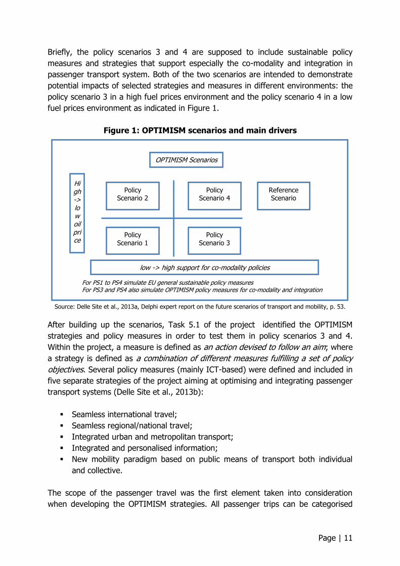
Briefly, the policy scenarios 3 and 4 are supposed to include sustainable policy

measures and strategies that support especially the co-modality and integration in

passenger transport system. Both of the two scenarios are intended to demonstrate

potential impacts of selected strategies and measures in different environments: the

policy scenario 3 in a high fuel prices environment and the policy scenario 4 in a low

fuel prices environment as indicated in Figure 1.

Figure 1: OPTIMISM scenarios and main drivers

Source: Delle Site et al., 2013a, Delphi expert report on the future scenarios of transport and mobility, p. 53.

After building up the scenarios, Task 5.1 of the project identified the OPTIMISM

strategies and policy measures in order to test them in policy scenarios 3 and 4.

Within the project, a measure is defined as an action devised to follow an aim; where

a strategy is defined as a combination of different measures fulfilling a set of policy

objectives. Several policy measures (mainly ICT-based) were defined and included in

five separate strategies of the project aiming at optimising and integrating passenger

transport systems (Delle Site et al., 2013b):

Seamless international travel;

Seamless regional/national travel;

Integrated urban and metropolitan transport;

Integrated and personalised information;

New mobility paradigm based on public means of transport both individual

and collective.

The scope of the passenger travel was the first element taken into consideration

when developing the OPTIMISM strategies. All passenger trips can be categorised

Policy Scenario 2

Policy Scenario 4

Policy

Scenario 1

Policy

Scenario 3

Reference Scenario

low -> high support for co-modality policies

High -> low oil price

For PS1 to PS4 simulate EU general sustainable policy measures

For PS3 and PS4 also simulate OPTIMISM policy measures for co-modality and integration

OPTIMISM Scenarios

Page | 12

into one of these three types of travel: urban/metropolitan, regional/national, and

international. The bigger the scope, the more complex and difficult is the integration

and optimisation of passenger transport systems. In fact they involve different

geographical/administrative/jurisdictional levels, and, therefore, different level of

required time and cost for their implementation.

Collection and provision of information is key to the optimisation of transport

systems, and therefore it was decided to develop a specific strategy aiming at

improving the transport information system and its services. The efficient use of

different modes on their own and in combination is the core idea of co-modality. The

current extremely spread use of private car is unsustainable and inefficient.

Therefore, the compelling offer of more efficient alternatives to the use of private

cars can significantly improve the overall efficiency and sustainability of passenger

transport systems. That is why the fifth strategy was proposed.

All strategies are described in terms of their co-modality objectives, functionalities

(ICT-based and Non-ICT-based measures), supporting measures (which identify

actions on the side of public policy to support the implementation of ICT-based and

non-ICT-based measures), and expected impacts on passengers’ travel choices.

The strategies consist of a common subset of co-modality measures selected from a

set of broader co-modality measures identified in task 5.1 (Delle Site et al., 2013b).

Instead of simulating the impacts of each OPTIMISM strategies, it was decided to

simulate the impacts of OPTIMISM co-modality measures implemented

simultaneously. Apart from this, impacts of individual strategies are assessed

qualitatively in Task 5.2 of the project separately.

Finally for the modelling exercise in this deliverable, the following policy measures

are included in policy scenarios 3 and 4 aiming to optimize passenger transport

system and support co-modality and integration:

Provision of travel Information

Integrated ticket and innovative ticketing

Improvement of luggage transport and passenger check-in

Innovative local mobility services

Improvement of mobility service at local level

Improvements at interchange points

Transport system infrastructure and rolling-stock improvements

As mentioned earlier, the other identified scenario variable is “energy prices” which

may follow two possible trends according to the project: the first is the baseline

trend (increasing) included in several EC studies (Christidis et al., 2010; European

Page | 13

Commission, 2011a; 2011b; 2012); the second is the Global Action trend (not

increasing) for oil prices defined in a study again by the EC (2011b).

The policy scenarios also include transport policy measures considered by the impact

assessment of the transport White Paper which are most likely to be implemented by

2030 especially in pricing, taxation and emission policies. Only different trends in fuel

prices brought a distinction in implementation of these policies for scenario

simulation. Different than the reference scenario and the policy scenarios 2 and 4, it

was decided to ensure internalization of external costs of road transport costs in an

increasing fuel prices environment in policy 1 and 3.

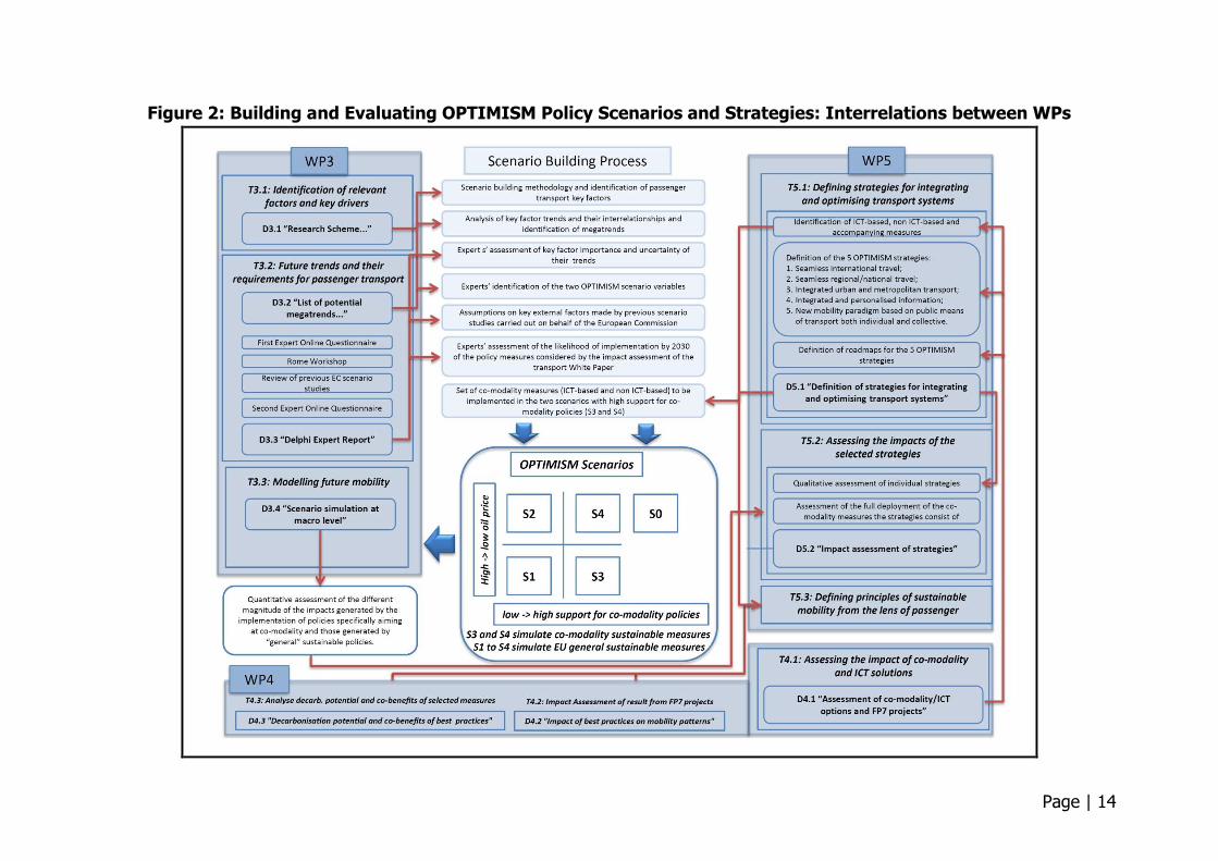
Further specification of scenarios and their implementation are discussed in section 4

after introducing the transport models used for the simulations. Figure 2 shows the

whole process for building and evaluating OPTIMISM policy scenarios and strategies

together with interrelations between the other project's WPs.

Page | 14

Figure 2: Building and Evaluating OPTIMISM Policy Scenarios and Strategies: Interrelations between WPs

Page | 15

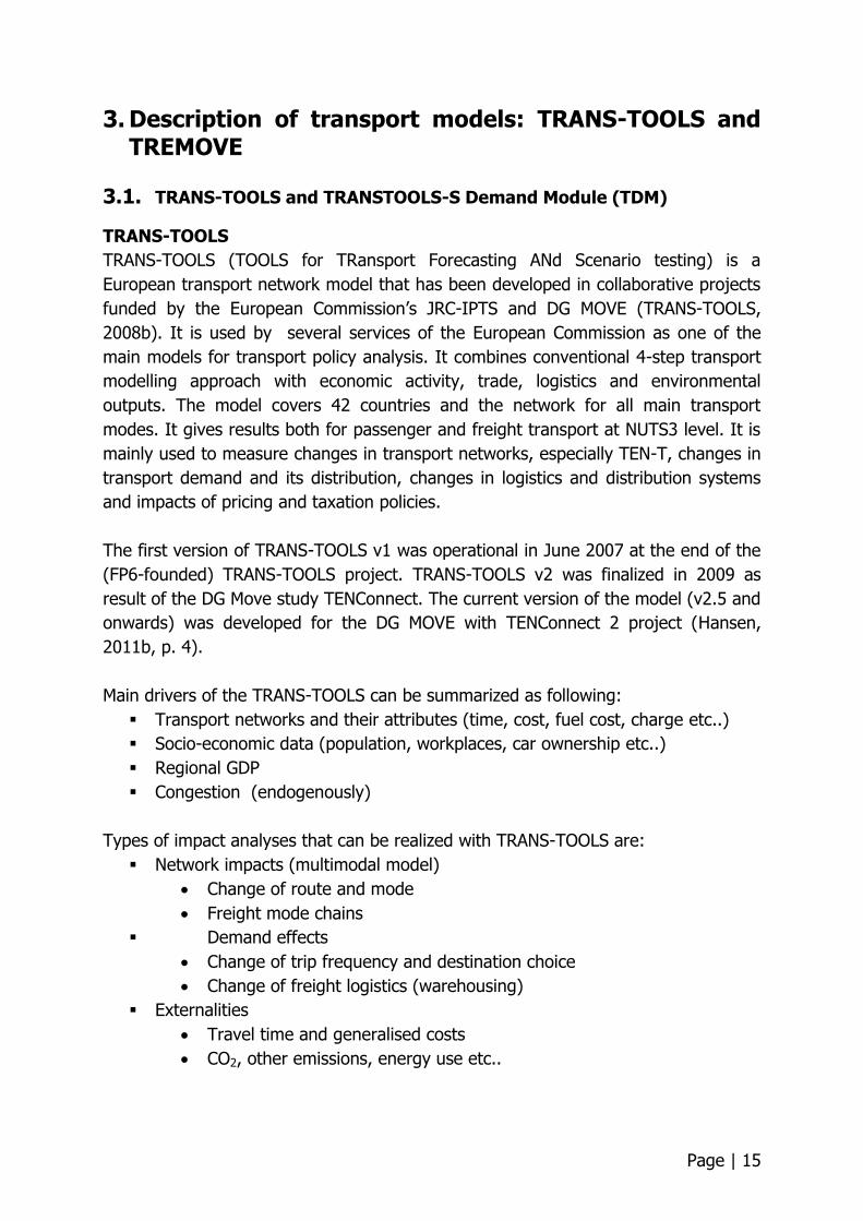
3. Description of transport models: TRANS-TOOLS and TREMOVE

3.1. TRANS-TOOLS and TRANSTOOLS-S Demand Module (TDM)

TRANS-TOOLS

TRANS-TOOLS (TOOLS for TRansport Forecasting ANd Scenario testing) is a

European transport network model that has been developed in collaborative projects

funded by the European Commission’s JRC-IPTS and DG MOVE (TRANS-TOOLS,

2008b). It is used by several services of the European Commission as one of the

main models for transport policy analysis. It combines conventional 4-step transport

modelling approach with economic activity, trade, logistics and environmental

outputs. The model covers 42 countries and the network for all main transport

modes. It gives results both for passenger and freight transport at NUTS3 level. It is

mainly used to measure changes in transport networks, especially TEN-T, changes in

transport demand and its distribution, changes in logistics and distribution systems

and impacts of pricing and taxation policies.

The first version of TRANS-TOOLS v1 was operational in June 2007 at the end of the

(FP6-founded) TRANS-TOOLS project. TRANS-TOOLS v2 was finalized in 2009 as

result of the DG Move study TENConnect. The current version of the model (v2.5 and

onwards) was developed for the DG MOVE with TENConnect 2 project (Hansen,

2011b, p. 4).

Main drivers of the TRANS-TOOLS can be summarized as following:

Transport networks and their attributes (time, cost, fuel cost, charge etc..)

Socio-economic data (population, workplaces, car ownership etc..)

Regional GDP

Congestion (endogenously)

Types of impact analyses that can be realized with TRANS-TOOLS are:

Network impacts (multimodal model)

Change of route and mode

Freight mode chains

Demand effects

Change of trip frequency and destination choice

Change of freight logistics (warehousing)

Externalities

Travel time and generalised costs

CO2, other emissions, energy use etc..

Page | 16

In addition to this, TRANS-TOOLS is capable of analysing any baseline or policy

scenario that can be specified within the assumptions or its exogenous data.

Conceptually, prospective scenarios could be categorized into 3 groups given as

below. Often scenarios being investigated can contain elements from all groups in

TRANS-TOOLS (Hansen, 2011a).

Economic development (such as high/low economic growth)

Infrastructure (major network analysis, TEN-T, corridor analysis etc..)

Strategy and policy (fiscal policies, taxation, regulatory scenarios etc..)

Further information on the model can be obtained through the documentation

available at its website (TRANS-TOOLS, 2008a). Since it is important for the

OPTIMISM scenario simulations, further information on its input output structure is

given in APPENDIX I.

TRANS-TOOLS-S and TRANS-TOOLS-S Demand Module (TDM):

TRANS-TOOLS-S, corresponds to a 'stripped-down' version of the original TRANS-

TOOLS model, a proof-of-concept prototype version developed by Joint Research

Centre of the European Commission. It is a tool that allows the assessment of the

impact of policy measures affecting a large number of drivers of transport demand,

transport volume, costs and the performance of the transport system as a whole.

The assumptions, modelling approach, operation and main results of the first phase

of development of this in-house transport network model is documented a report

with the name of "TRANS-TOOLS-S: A comprehensive approach for an EU transport

network model" (Vannacci et al., 2013). Based on this documentation, a brief

description of the model can be given as follows:

The TRANS-TOOLS-S model uses a simplified architecture and concentrates on the

issues directly relevant to transport demand and the performance of the transport

networks. Its main characteristics can be summarized as below (Vannacci et al.,

2013, p.2):

Matrix based structure, based on origin-destination matrices at NUTS3 level,

Disaggregate formulation of transport demand equations per mode and type

of trip,

Demand linked to socio-economic drivers and levels of economic activity;

possibility of further detail in demand equations through the inclusion of

additional variables,

Assignment to the network keeps previous TRANS-TOOLS versions' module

(Traffic Analyst); possibility to replace with third-party assignment algorithms,

Improved treatment of road congestion through capacity constraints;

possibility to apply congestion simulation in other modes,

Page | 17

Iterative approach allows user-defined level of convergence of model results

Flexibility in definition of policy relevant indicators,

Possibility to connect with economic, fleet and energy models.

The main conceptual difference between TRANS-TOOLS and this stripped-down

version (TRANS-TOOLS-S) is the selection of a more comprehensive approach in

connecting the various model elements between them. Whereas the original TRANS-

TOOLS included several modules by different developers each addressing a specific

issue independently, TRANS-TOOLS-S uses a leaner structure, expressing all model

relationships in an easy to follow interconnected matrix structure. This allows a

transparent process and minimizes the risk of bad communication between the

various modules. TRANS-TOOLS-S follows conceptually the same standard transport

model as adopted in TRANS-TOOLS, namely the widely accepted 4-step model

approach, trip generation, trip distribution, mode choice and traffic assignment

in a stylized fashion allowing for a simpler method of calibration and alignment with

EUROSTAT statistics. The development process involved an iterative process of

combining the simplified (matrix based) model structure and (TEN-T based) networks

with the improved demand, assignment and reporting modules. The new tool builds

on three main building blocks that are linked with clear and robust algorithms and

maintain a coherent structure that allows future improvements and connections with

other tools and models (Vannacci et al., 2013, p.3):

a) A demand module for passenger and freight transport disaggregated at

NUTS3 level using an Origin-Destination (O-D) matrix structure: the matrices

are an important building block that allow the analysis of transport demand

and costs for each mode and trip purpose, but also by distance class.

b) Transport networks that reflect the actual policy requirements without adding

excessive operational complications: the networks used by the model are

based on the comprehensive networks of the TEN-T.

c) An improved assignment algorithm that allocates the demand (from the

origin-destination matrices) to the transport networks (comprehensive TEN-T

networks) in an operationally efficient manner.

For the simulation of OPTIMISM policy scenarios, only the first step

- TRANS-TOOLS-S Demand Module (TDM) - of the model was used. Considering the

OPTIMISM policy scenario structure and the policies to be tested, country based

estimations of demand with corresponding modal shifts were found sufficient.

Therefore, transport activity indicators at year 2030 for each policy scenarios were

only estimated at country level, without any assignment to the network links and

without distribution of demand to the NUTS 3 regions.

Page | 18

The structure of TRANS-TOOLS-S Demand Module is mainly based on the GLADYSTE

Model (Hidalgo et al., 2011). It was further improved for scenario simulation in

OPTIMISM using up-to-date data from the latest TRANS-TOOLS versions and from

the ETIS+ database. It was also recalibrated to ensure having parallel results with

the EUROSTAT data for 2010 and with the EC baseline scenario for 2030. The

structure of the demand module and the logic behind it can be seen in GLADYSTE

Model report (Hidalgo et al., 2011). The specific section for its demand module is

also given in the APPENDIX II including the main assumptions and equations of the

module.

3.2. TREMOVE and TREMOVE SYSTEM DYNAMICS (TSD)

This section includes description of TREMOVE and TREMOVE System Dynamics

model which the latter was used to measure environmental impacts of OPTIMISM

policy scenarios. TSD model is a simplified, system dynamic version of TREMOVE

model used since years to assess the impacts of European Commission’s transport

policies. The next section starts with a short introduction of TREMOVE model

followed by TSD. This presentation will allow readers to understand the objectives,

the purposes and the use of both TREMOVE and TSD models as well as the

differences between them. The sub-sections will also explain the reason for using

TSD instead of TREMOVE model.

TREMOVE Model

TREMOVE (De Ceuster, et al. 2007) is a transport and emissions simulation model

developed for the European Commission, to be able to make policy assessments in

transport sector and to be able to measure effects of different transport and

environment policies on the emissions of the transport sector. It is an integrated

simulation model developed for the strategic analysis of the costs and effects of a

wide range of policy instruments and measures applicable to local, regional, and

European transport markets.

TREMOVE covers 31 countries and 8 sea regions. All relevant transport modes are

modelled, including air and long-distance maritime transport. The model covers the

period between 1995-2030 with yearly intervals. The TREMOVE model consists of

separate country models. While the numeric values of the model differ from country

to country, the model code distinguished into four linked module, is identical across

countries.

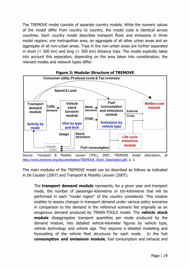
Figure 3 shows the modular structure of TREMOVE. The model performs a year-by-

year loop over its modules. The same modules are used for both the construction of

the baseline scenario as for the evaluation of policy scenarios.

Page | 19

The TREMOVE model consists of separate country models. While the numeric values

of the model differ from country to country, the model code is identical across

countries. Each country model describes transport flows and emissions in three

model regions: one metropolitan area, an aggregate of all other urban areas and an

aggregate of all non-urban areas. Trips in the non-urban areas are further separated

in short (< 500 km) and long (> 500 km) distance trips. The model explicitly takes

into account this separation, depending on the area taken into consideration, the

relevant modes and network types differ.

Figure 3: Modular Structure of TREMOVE

Vehicle stock

turnover module

Vkm by type

and tech

Fuel consumption

and emissions module

Emissions by vehicle type

Traffic

demand

Stock

structure

Usage

Usage Stock structure

Fuel consumption Usage Cost

Speed & Load

Transport demand module

Activity by mode

Welfare cost module

Life cycle emissions

module

Consumer utility, Producer costs & Tax revenues

External

Costs

Source: Transport & Mobility Leuven (TML), 2007, TREMOVE model description, at

http://www.tremove.org/documentation/TREMOVE_Short_Description.pdf, p. 2.

The main modules of the TREMOVE model can be described as follows as indicated

in De Ceuster (2007) and Transport & Mobility Leuven (2007):

The transport demand module represents, for a given year and transport

mode, the number of passenger-kilometres or ton-kilometres that will be

performed in each “model region” of the country considered. This module

enables to assess changes in transport demand under various policy scenarios

in comparison to the demand in the reference scenario fed originally as an

exogenous demand produced by TRANS-TOOLS model. The vehicle stock

module disaggregates transport quantities per mode produced by the

demand module, into detailed vehicle-kilometer figures by vehicle type,

vehicle technology and vehicle age. This requires a detailed modelling and

forecasting of the vehicle fleet structures for each mode. In the fuel

consumption and emissions module, fuel consumption and exhaust and

http://www.tremove.org/documentation/TREMOVE_Short_Description.pdf

Page | 20

evaporative emissions are calculated for all modes. Emission factors have

been derived consistently from EU sources, thus might deviate from national

estimates. Finally, to evaluate policies in TREMOVE, the welfare

assessment module has been constructed. Differences in welfare between

the baseline and the simulated policy scenarios are calculated.

Tremove System Dynamics (TSD)

TREMOVE System Dynamics abbreviated as TSD is a simplified, System Dynamic

model version of TREMOVE. TSD basically replicates the TREMOVE vehicle stock and

emissions modules, while the demand input is fully exogenous, i.e. transport demand

produced by TRANS-TOOLS model.

TSD has been developed during the GLADYSTE project1 of the European Commission

Joint Research Centre, Institute for Prospective Technological Studies. The data

required by TSD are taken from the current TREMOVE version 3.3.1. It was

developed during the iTREN-2030: Integrated Transport and Energy Baseline until

2030 project (Schade and Krail, 2010). During the GLADYSTE project, the baseline

results on emissions, fuel consumption and vehicle fleet stocks of TSD have been

fully calibrated to that TREMOVE version, i.e. using results of the reference scenario

of the iTREN-2030 project, as well as TSD model reactions to policy measures.

In TSD, the transport demand fed exogenously is sent to a demand segmentation

module, in which transport demand is further disaggregated using a range of

techniques from simple allocation keys to full logit functions. TSD requires exogenous

datasets representing transport demand. Basically demand data and forecast in term

of vehicles-kilometres and passenger-kilometres are needed. Such dataset must

include yearly demand data of the five transport mode categories in TREMOVE model

(air, rail, inland water ways, road, and metro-tram) for the whole period between

2000 and 2030.

One of the main differences between TREMOVE and TSD is found in this demand

module. TSD does not allow assessing changes in transport demand due to policy

measures. The model takes simply transport demand as it is delivered by TRANS-

TOOLS model. Transport demand is fed to TSD model and proceeds directly to the

vehicle stock module where the calculation of the fleet dynamics is conducted. All

demand changes due to prices changes due to technological measures and new

taxation or regulation policies are assumed to completely happen in the transport

model (TRANS-TOOLS).

1 GLADYSTE project internet page: http://www.tmleuven.be/project/tremovegladyste/home.htm as accessed on 24 September 2013.

http://www.tmleuven.be/project/tremovegladyste/home.htm

Page | 21

The vehicle stock module is split in 2 sub modules: transport costs and fleet

planning. The transport costs module holds a detailed breakdown of the costs of

transport, ranging from purchase cost over different kinds of taxes to labour cost.

The detailed cost breakdown allows for detailed policy analysis influencing specific

elements of transport cost. The fleet planning module focuses on the fleet dynamics

and includes a copy of the TREMOVE sales logit for passenger cars and light duty

trucks.

Finally, the emissions module is somewhat simplified compared to TREMOVE; instead

of including the full COPERT IV functions in the model code, emission factors, at the

highest level of detail, are determined in an offline setting and introduced in the

model as input. This approach is chosen as it simplifies the model and little feedback

exists between other parts of the module and the emission factors (apart from fuel

consumption and related pollutants, which is taken into account). Moreover, this

approach allows for changing emission factor directly at the input, so it is easier to

update the emission factors when new research is available.

Considering the characteristics of the OPTIMISM policy scenario simulations, which

are mainly based on changes in fuel prices and transport costs to capture impacts of

internalizations and co-modality measures, both of the TREMOVE and TSD models

could have been used. However, since TSD has computational advantages in terms

of model running time, and since the transport demand is estimated by TRANS-

TOOLS, it was decided to use TSD for modelling only environmental impacts of the

policy scenarios.

Page | 22

4. Specification of OPTIMISM scenarios for modelling exercise

The main characteristics of the OPTIMISM policy scenarios were already introduced

in section 2 of this deliverable based on the information provided by previous tasks

of the project. Here in section 4, further refinement and specification of the scenarios

are introduced with their implementation steps in modelling with TRANSTOOLS-S

Demand Module (TDM) and TREMOVE System Dynamics (TSD).

The simulation process of OPTIMISM scenarios was divided into two steps: at first,

the TDM was used to estimate transport activity for 2030 for all policy scenarios

including passenger and ton kilometres for all modes; than the output of TDM

(mainly country based transport activities and modal shares) was used as an input to

TSD simulations for estimating transport emissions and vehicle fleet sizes for each

policy scenarios.

Before starting to specify policy scenarios to estimate transport activity, it is worth

mentioning the reference scenario for 2030 and the main socio-economic variables

used in the scenario simulations:

The reference scenario for transport activity was derived from a recent study

conducted by the European Commission (2012): "2012 EU Reference Scenario

modelling - Draft transport activity projections". The reference scenario

described in this study includes transport activity estimations for all EU

countries for all main types of transport modes. Two models were used for

developing the transport activity projections in the reference scenario:

TRANSTOOLS and the PRIMES-TREMOVE models. Both models are managed

by the TranScenario consortium mainly by experts from DG ENER, DG MOVE

and DG CLIMA of the European Commission. The reference scenario of the

TDM in OPTIMISM was calibrated according to the TranScenario estimations

on transport activity.

In addition to this, main variables of the models such as GDP, population and

baseline oil prices used in the policy scenario simulations are also directly

taken from the TranScenario reference scenario for 2030. The projections for

GDP and population used in the reference scenario and in the OPTIMISM

policy scenario simulations are given in APPENDIX 3.

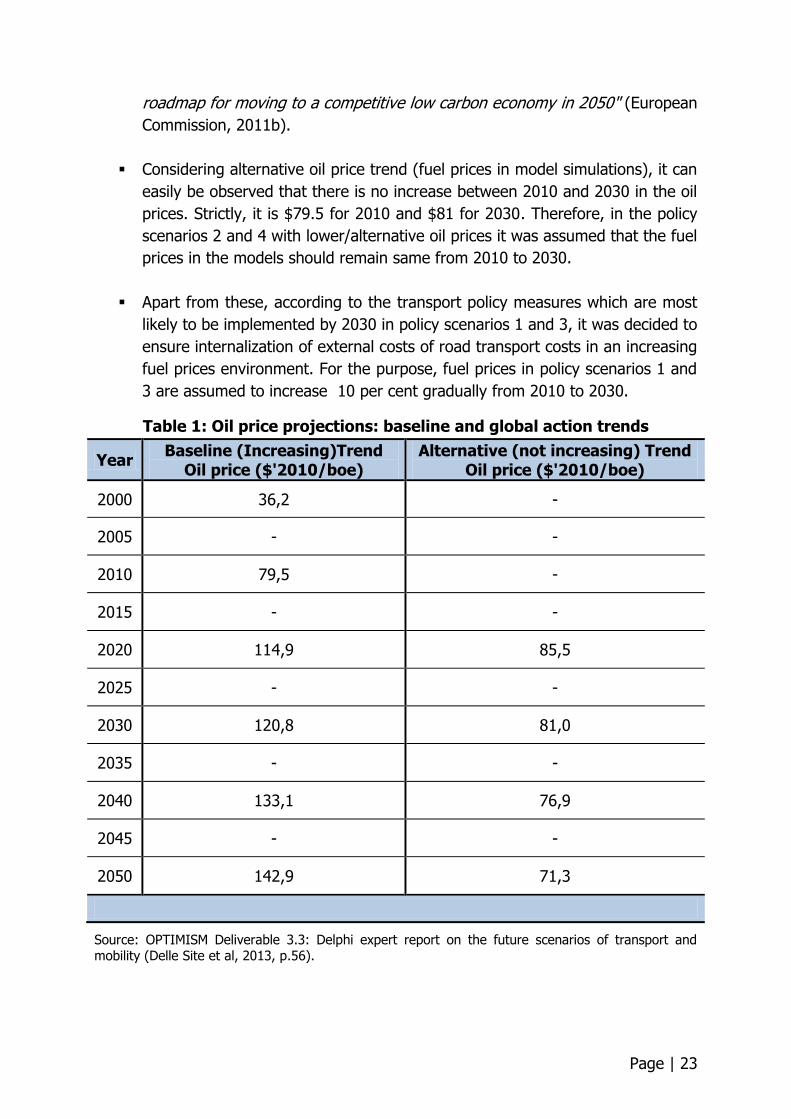
As mentioned earlier, the oil prices follow two different trends in policy

scenarios as shown in Table 1. The baseline trend (increasing) is derived from

the TranScenario study (European Commision, 2012), and the alternative

trend (global action scenario/not increasing) is derived from another study: "a

Page | 23

roadmap for moving to a competitive low carbon economy in 2050" (European

Commission, 2011b).

Considering alternative oil price trend (fuel prices in model simulations), it can

easily be observed that there is no increase between 2010 and 2030 in the oil

prices. Strictly, it is $79.5 for 2010 and $81 for 2030. Therefore, in the policy

scenarios 2 and 4 with lower/alternative oil prices it was assumed that the fuel

prices in the models should remain same from 2010 to 2030.

Apart from these, according to the transport policy measures which are most

likely to be implemented by 2030 in policy scenarios 1 and 3, it was decided to

ensure internalization of external costs of road transport costs in an increasing

fuel prices environment. For the purpose, fuel prices in policy scenarios 1 and

3 are assumed to increase 10 per cent gradually from 2010 to 2030.

Table 1: Oil price projections: baseline and global action trends

Year Baseline (Increasing)Trend

Oil price ($'2010/boe) Alternative (not increasing) Trend

Oil price ($'2010/boe)

2000 36,2 -

2005 - -

2010 79,5 -

2015 - -

2020 114,9 85,5

2025 - -

2030 120,8 81,0

2035 - -

2040 133,1 76,9

2045 - -

2050 142,9 71,3

Source: OPTIMISM Deliverable 3.3: Delphi expert report on the future scenarios of transport and mobility (Delle Site et al, 2013, p.56).

Page | 24

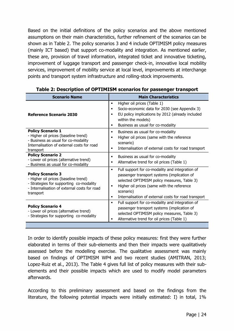
Based on the initial definitions of the policy scenarios and the above mentioned

assumptions on their main characteristics, further refinement of the scenarios can be

shown as in Table 2. The policy scenarios 3 and 4 include OPTIMISM policy measures

(mainly ICT based) that support co-modality and integration. As mentioned earlier,

these are, provision of travel information, integrated ticket and innovative ticketing,

improvement of luggage transport and passenger check-in, innovative local mobility

services, improvement of mobility service at local level, improvements at interchange

points and transport system infrastructure and rolling-stock improvements.

Table 2: Description of OPTIMISM scenarios for passenger transport

Scenario Name Main Characteristics

Reference Scenario 2030

Higher oil prices (Table 1)

Socio-economic data for 2030 (see Appendix 3)

EU policy implications by 2012 (already included

within the models)

Business as usual for co-modality

Policy Scenario 1

- Higher oil prices (baseline trend)

- Business as usual for co-modality Internalisation of external costs for road

transport


Higher oil prices (same with the reference

scenario)

Internalisation of external costs for road transport

Policy Scenario 2 - Lower oil prices (alternative trend)

- Business as usual for co-modality


Alternative trend for oil prices (Table 1)

Policy Scenario 3

- Higher oil prices (baseline trend) - Strategies for supporting co-modality

- Internalisation of external costs for road transport

Full support for co-modality and integration of

passenger transport systems (implication of

selected OPTIMISM policy measures, Table 3)

Higher oil prices (same with the reference

scenario)

Internalisation of external costs for road transport

Policy Scenario 4

- Lower oil prices (alternative trend) - Strategies for supporting co-modality

Full support for co-modality and integration of

passenger transport systems (implication of

selected OPTIMISM policy measures, Table 3)

Alternative trend for oil prices (Table 1)

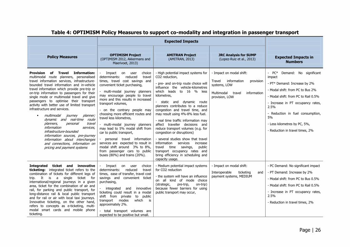
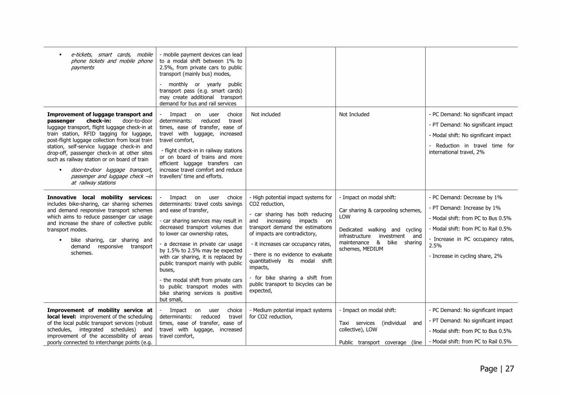
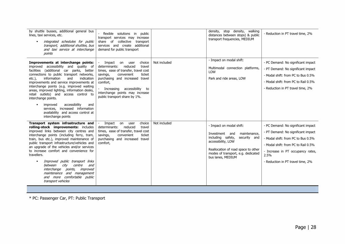
In order to identify possible impacts of these policy measures: first they were further

elaborated in terms of their sub-elements and then their impacts were qualitatively

assessed before the modelling exercise. The qualitative assessment was mainly

based on findings of OPTIMISM WP4 and two recent studies (AMITRAN, 2013;

Lopez-Ruiz et al., 2013). The Table 4 gives full list of policy measures with their sub-

elements and their possible impacts which are used to modify model parameters

afterwards.

According to this preliminary assessment and based on the findings from the

literature, the following potential impacts were initially estimated: I) in total, 1%

Page | 25

decrease in private car demand, 5% increase in public bus and rail demand, II) in

average, 5%-10% increase in travel per person by public bus and rail, and IV)

additionally, 10% decrease in public transport travel times/transport costs.

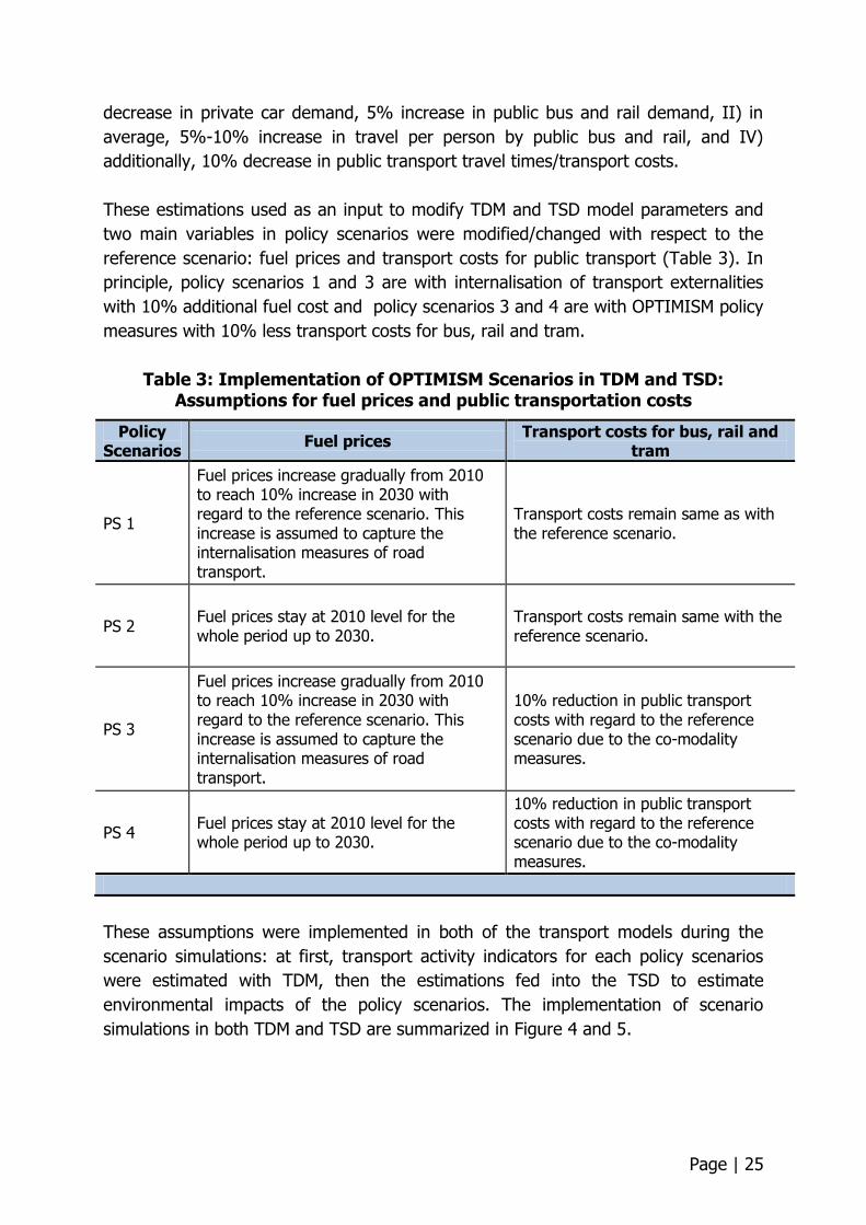
These estimations used as an input to modify TDM and TSD model parameters and

two main variables in policy scenarios were modified/changed with respect to the

reference scenario: fuel prices and transport costs for public transport (Table 3). In

principle, policy scenarios 1 and 3 are with internalisation of transport externalities

with 10% additional fuel cost and policy scenarios 3 and 4 are with OPTIMISM policy

measures with 10% less transport costs for bus, rail and tram.

Table 3: Implementation of OPTIMISM Scenarios in TDM and TSD: Assumptions for fuel prices and public transportation costs

Policy Scenarios

Fuel prices Transport costs for bus, rail and

tram

PS 1

Fuel prices increase gradually from 2010 to reach 10% increase in 2030 with regard to the reference scenario. This increase is assumed to capture the internalisation measures of road transport.

Transport costs remain same as with the reference scenario.

PS 2 Fuel prices stay at 2010 level for the whole period up to 2030.

Transport costs remain same with the reference scenario.

PS 3

Fuel prices increase gradually from 2010 to reach 10% increase in 2030 with regard to the reference scenario. This increase is assumed to capture the internalisation measures of road transport.

10% reduction in public transport costs with regard to the reference scenario due to the co-modality measures.

PS 4 Fuel prices stay at 2010 level for the whole period up to 2030.

10% reduction in public transport costs with regard to the reference scenario due to the co-modality measures.

These assumptions were implemented in both of the transport models during the

scenario simulations: at first, transport activity indicators for each policy scenarios

were estimated with TDM, then the estimations fed into the TSD to estimate

environmental impacts of the policy scenarios. The implementation of scenario

simulations in both TDM and TSD are summarized in Figure 4 and 5.

Page | 26

Table 4: OPTIMISM Policy Measures to support co-modality and integration in passenger transport

Policy Measures

Expected Impacts

Expected Impacts in Numbers

OPTIMISM Project

(OPTIMISM 2012, Akkermans and Maerivoet, 2013)

AMITRAN Project (AMITRAN, 2013)

JRC Analysis for SUMP (Lopez-Ruiz et al., 2013)

Provision of Travel Information: multimodal route planners, personalised travel information services, infrastructure-bounded travel information and in-vehicle travel information which provide pre-trip or on-trip information to passengers for their single mode or multimodal travel and give passengers to optimise their transport activity with better use of limited transport infrastructure and services.

multimodal journey planner; dynamic and real-time route planners, personal travel information services, infrastructure-bounded information sources, pre-journey information about interchanges and connections, information on pricing and payment systems

- Impact on user choice determinants: reduced travel times, travel cost savings and convenient ticket purchasing,

- multi-modal journey planners may encourage people to travel more and this results in increased transport volumes,

- on the contrary people may choosing more efficient routes and travel less kilometres,

- multi-modal journey planners may lead to 5% modal shift from car to public transport,

- personal travel information services are expected to result in modal shift around 3% to 8%, from passenger cars to public buses (80%) and trains (20%).

- High potential impact systems for CO2 reduction,

- pre- and on-trip route choice will influence the vehicle-kilometres which leads to 16 % less kilometres,

- static and dynamic route planners contributes to a reduce congestion and travel time, and may result using 4%-8% less fuel.

- real time traffic information may affect traveller decisions and reduce transport volumes (e.g. for congestion or disruptions)

- several studies show that travel information services increase travel time savings, public transport occupancy rates and bring efficiency in scheduling and capacity usage.

- Impact on modal shift: Travel information provision systems, LOW Multimodal travel information provision, LOW

- PC* Demand: No significant impact

- PT* Demand: Increase by 2%

- Modal shift: from PC to Bus 2%

- Modal shift: from PC to Rail 0.5%

- Increase in PT occupancy rates, 2.5%

- Reduction in fuel consumption, 5%

- Less kilometres by PC, 5%,

- Reduction in travel times, 2%

Integrated ticket and innovative ticketing: integrated ticket refers to the combination of tickets for different legs of trip. It is a single ticket for international/regional journeys in a given area, ticket for the combination of air and rail, for parking and public transport, for long-distance rail & local public transport and for rail or air with local taxi journeys. Innovative ticketing, on the other hand, refers to concepts as e-ticketing, multi-modal smart cards and mobile phone ticketing.

- Impact on user choice determinants: reduced travel times, ease of transfer, travel cost savings and convenient ticket purchasing,

- integrated and innovative ticketing could result in a modal shift from private to public transport modes which is approximately 2%.

- total transport volumes are expected to be positive but small.

- Medium potential impact systems for CO2 reduction

- the system will have an influence on all kind of mode choice (strategic, pre-trip, on-trip) because fewer barriers for using public transport may occur,

- Impact on modal shift:

Interoperable ticketing and payment systems, MEDIUM

- PC Demand: No significant impact

- PT Demand: Increase by 2%

- Modal shift: from PC to Bus 0.5%



- Reduction in travel times, 2%

Page | 27

e-tickets, smart cards, mobile phone tickets and mobile phone payments

- mobile payment devices can lead to a modal shift between 1% to 2.5%, from private cars to public transport (mainly bus) modes,

- monthly or yearly public transport pass (e.g. smart cards) may create additional transport demand for bus and rail services

Improvement of luggage transport and passenger check-in: door-to-door luggage transport, flight luggage check-in at train station, RFID tagging for luggage, post-flight luggage collection from local train station, self-service luggage check-in and drop-off, passenger check-in at other sites such as railway station or on board of train

door-to-door luggage transport, passenger and luggage check –in at railway stations

- Impact on user choice determinants: reduced travel times, ease of transfer, ease of travel with luggage, increased travel comfort,

- flight check-in in railway stations or on board of trains and more efficient luggage transfers can increase travel comfort and reduce travellers’ time and efforts.

Not included Not Included - PC Demand: No significant impact

- PT Demand: No significant impact

- Modal shift: No significant impact

- Reduction in travel time for international travel, 2%

Innovative local mobility services: includes bike-sharing, car sharing schemes and demand responsive transport schemes which aims to reduce passenger car usage and increase the share of collective public transport modes.

bike sharing, car sharing and demand responsive transport schemes.

- Impact on user choice determinants: travel costs savings and ease of transfer,

- car sharing services may result in decreased transport volumes due to lower car ownership rates,

- a decrease in private car usage by 1.5% to 2.5% may be expected with car sharing, it is replaced by public transport mainly with public buses,

- the modal shift from private cars to public transport modes with bike sharing services is positive but small,

- High potential impact systems for CO2 reduction,

- car sharing has both reducing and increasing impacts on transport demand the estimations of impacts are contradictory,

- it increases car occupancy rates,

- there is no evidence to evaluate quantitatively its modal shift impacts,

- for bike sharing a shift from public transport to bicycles can be expected,

- Impact on modal shift: Car sharing & carpooling schemes, LOW Dedicated walking and cycling infrastructure investment and maintenance & bike sharing schemes, MEDIUM

- PC Demand: Decrease by 1%

- PT Demand: Increase by 1%



- Increase in PC occupancy rates, 2.5%

- Increase in cycling share, 2%

Improvement of mobility service at local level: improvement of the scheduling of the local public transport services (robust schedules, integrated schedules) and improvement of the accessibility of areas poorly connected to interchange points (e.g.

- Impact on user choice determinants: reduced travel times, ease of transfer, ease of travel with luggage, increased travel comfort,

- Medium potential impact systems for CO2 reduction,

- Impact on modal shift: Taxi services (individual and collective), LOW Public transport coverage (line





Page | 28

by shuttle busses, additional general bus lines, taxi services, etc.

integrated schedules for public transport, additional shuttles, bus and taxi service at interchange points

- flexible solutions in public transport services may increase share of collective transport services and create additional demand for public transport

density, stop density, walking distances between stops) & public transport frequencies, MEDIUM

- Reduction in PT travel time, 2%

Improvements at interchange points: improved accessibility and quality of facilities (additional car parks, better connections to public transport networks, etc.), information and indication improvements and service improvements at interchange points (e.g. improved waiting areas, improved lighting, information desks, retail outlets) and access control to interchange points.

improved accessibility and services, increased information availability and access control at interchange points

- Impact on user choice determinants: reduced travel times, ease of transfer, travel cost savings, convenient ticket purchasing and increased travel comfort,

- Increasing accessibility to interchange points may increase public transport share by 1%.

Not included - Impact on modal shift: Multimodal connection platforms, LOW

Park and ride areas, LOW






Transport system infrastructure and rolling-stock improvements: includes improved links between city centres and interchange points (including ferry, tram, train, bus etc.), improved maintenance of public transport infrastructure/vehicles and an upgrade of the vehicles and/or services to increase comfort and convenience for travellers.

Improved public transport links between city centre and interchange points, improved maintenance and management and more comfortable public transport vehicles

- Impact on user choice determinants: reduced travel times, ease of transfer, travel cost savings, convenient ticket purchasing and increased travel comfort,

Not included - Impact on modal shift: Investment and maintenance, including safety, security and accessibility, LOW Reallocation of road space to other modes of transport, e.g. dedicated bus lanes, MEDIUM







* PC: Passenger Car, PT: Public Transport

Page | 29

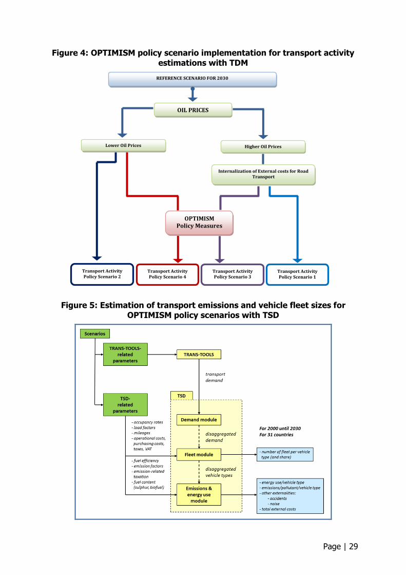
Figure 4: OPTIMISM policy scenario implementation for transport activity

estimations with TDM

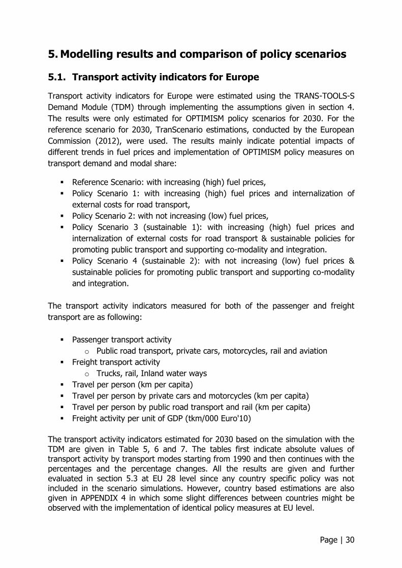
Figure 5: Estimation of transport emissions and vehicle fleet sizes for OPTIMISM policy scenarios with TSD

REFERENCE SCENARIO FOR 2030

OIL PRICES

Higher Oil Prices

Lower Oil Prices

OPTIMISM Policy Measures

Internalization of External costs for Road Transport

Transport Activity Policy Scenario 1




Page | 30

5. Modelling results and comparison of policy scenarios

5.1. Transport activity indicators for Europe

Transport activity indicators for Europe were estimated using the TRANS-TOOLS-S

Demand Module (TDM) through implementing the assumptions given in section 4.

The results were only estimated for OPTIMISM policy scenarios for 2030. For the

reference scenario for 2030, TranScenario estimations, conducted by the European

Commission (2012), were used. The results mainly indicate potential impacts of

different trends in fuel prices and implementation of OPTIMISM policy measures on

transport demand and modal share:

Reference Scenario: with increasing (high) fuel prices,

Policy Scenario 1: with increasing (high) fuel prices and internalization of

external costs for road transport,

Policy Scenario 2: with not increasing (low) fuel prices,

Policy Scenario 3 (sustainable 1): with increasing (high) fuel prices and

internalization of external costs for road transport & sustainable policies for

promoting public transport and supporting co-modality and integration.

Policy Scenario 4 (sustainable 2): with not increasing (low) fuel prices &

sustainable policies for promoting public transport and supporting co-modality

and integration.

The transport activity indicators measured for both of the passenger and freight

transport are as following:

Passenger transport activity

o Public road transport, private cars, motorcycles, rail and aviation

Freight transport activity

o Trucks, rail, Inland water ways

Travel per person (km per capita)

Travel per person by private cars and motorcycles (km per capita)

Travel per person by public road transport and rail (km per capita)

Freight activity per unit of GDP (tkm/000 Euro'10)

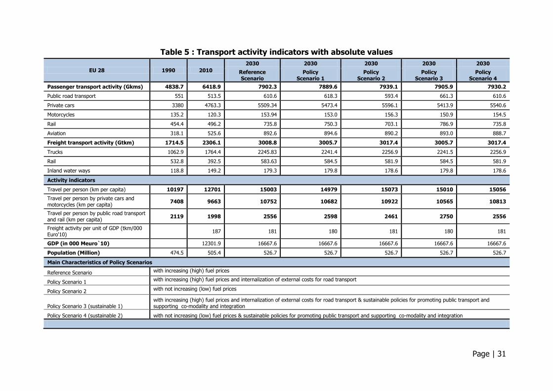
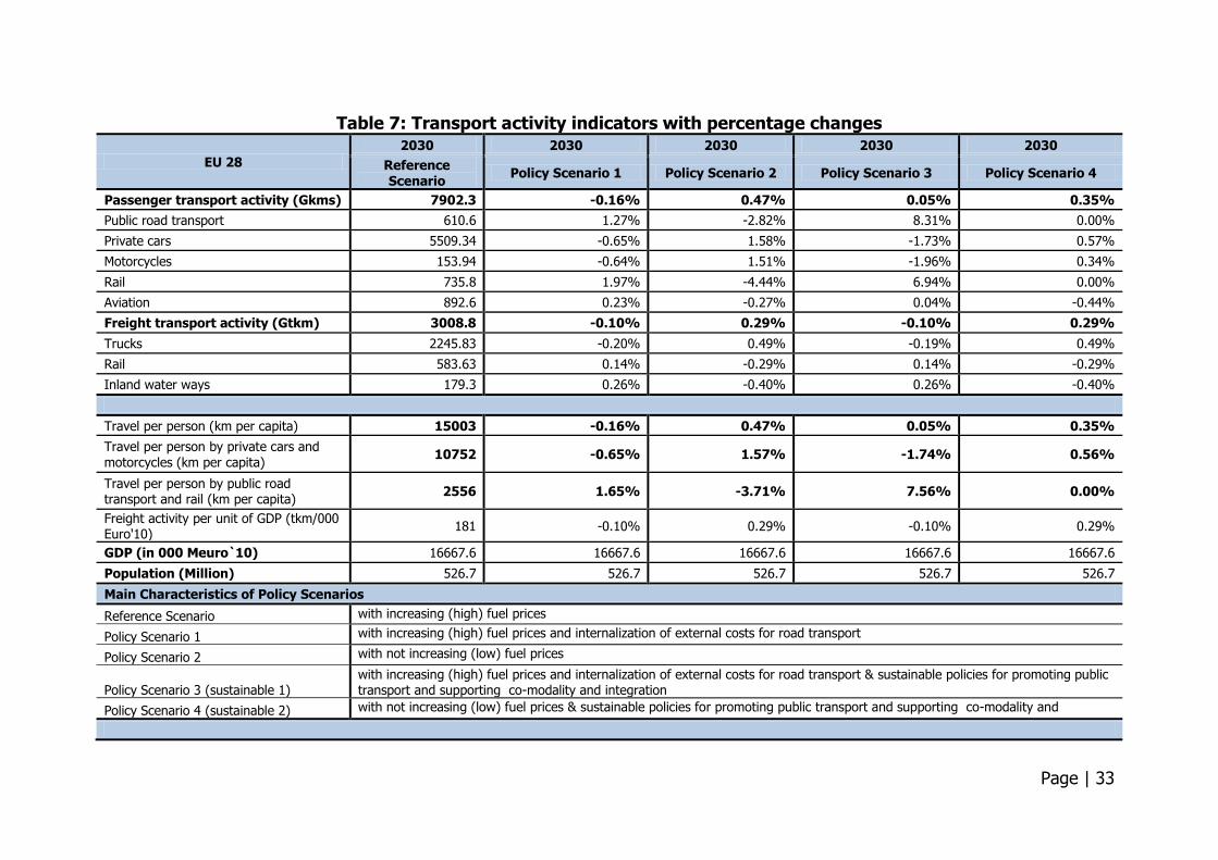
The transport activity indicators estimated for 2030 based on the simulation with the TDM are given in Table 5, 6 and 7. The tables first indicate absolute values of transport activity by transport modes starting from 1990 and then continues with the percentages and the percentage changes. All the results are given and further evaluated in section 5.3 at EU 28 level since any country specific policy was not included in the scenario simulations. However, country based estimations are also given in APPENDIX 4 in which some slight differences between countries might be observed with the implementation of identical policy measures at EU level.

Page | 31

Table 5 : Transport activity indicators with absolute values

EU 28 1990 2010

2030 2030 2030 2030 2030

Reference Scenario

Policy Scenario 1

Policy Scenario 2

Policy Scenario 3

Policy Scenario 4

Passenger transport activity (Gkms) 4838.7 6418.9 7902.3 7889.6 7939.1 7905.9 7930.2

Public road transport 551 513.5 610.6 618.3 593.4 661.3 610.6

Private cars 3380 4763.3 5509.34 5473.4 5596.1 5413.9 5540.6

Motorcycles 135.2 120.3 153.94 153.0 156.3 150.9 154.5

Rail 454.4 496.2 735.8 750.3 703.1 786.9 735.8

Aviation 318.1 525.6 892.6 894.6 890.2 893.0 888.7

Freight transport activity (Gtkm) 1714.5 2306.1 3008.8 3005.7 3017.4 3005.7 3017.4

Trucks 1062.9 1764.4 2245.83 2241.4 2256.9 2241.5 2256.9

Rail 532.8 392.5 583.63 584.5 581.9 584.5 581.9

Inland water ways 118.8 149.2 179.3 179.8 178.6 179.8 178.6

Activity indicators

Travel per person (km per capita) 10197 12701 15003 14979 15073 15010 15056


7408 9663 10752 10682 10922 10565 10813


2119 1998 2556 2598 2461 2750 2556


187 181 180 181 180 181

GDP (in 000 Meuro`10) 12301.9 16667.6 16667.6 16667.6 16667.6 16667.6

Population (Million) 474.5 505.4 526.7 526.7 526.7 526.7 526.7

Main Characteristics of Policy Scenarios

Reference Scenario with increasing (high) fuel prices

Policy Scenario 1 with increasing (high) fuel prices and internalization of external costs for road transport Policy Scenario 2 with not increasing (low) fuel prices

Policy Scenario 3 (sustainable 1) with increasing (high) fuel prices and internalization of external costs for road transport & sustainable policies for promoting public transport and supporting co-modality and integration

Policy Scenario 4 (sustainable 2) with not increasing (low) fuel prices & sustainable policies for promoting public transport and supporting co-modality and integration

Page | 32

Table 6: Transport activity Indicators with percentages

EU 28 1990 2010

2030 2030 2030 2030 2030

Reference Scenario

Policy Scenario 1

Policy Scenario 2

Policy Scenario 3

Policy Scenario 4

Passenger transport activity (Gkms)

100% 100% 100% 100% 100% 100% 100%

Public road transport 11.4% 8.0% 7.7% 7.8% 7.5% 8.4% 7.7%

Private cars 69.9% 74.2% 69.7% 69.4% 70.5% 68.5% 69.9%

Motorcycles 2.8% 1.9% 1.9% 1.9% 2.0% 1.9% 1.9%

Rail 9.4% 7.7% 9.3% 9.5% 8.9% 10.0% 9.3%

Aviation 6.6% 8.2% 11.3% 11.3% 11.2% 11.3% 11.2%

Freight transport activity (Gtkm) 100% 100% 100% 100% 100% 100% 100%

Trucks 62.0% 76.5% 74.6% 74.6% 74.8% 74.6% 74.8%

Rail 31.1% 17.0% 19.4% 19.4% 19.3% 19.4% 19.3%

Inland water ways 6.9% 6.5% 6.0% 6.0% 5.9% 6.0% 5.9%



Policy Scenario 1 with increasing (high) fuel prices and internalization of external costs for road transport

Policy Scenario 2 with not increasing (low) fuel prices



Page | 33

Table 7: Transport activity indicators with percentage changes

EU 28

2030 2030 2030 2030 2030

Reference Scenario

Policy Scenario 1 Policy Scenario 2 Policy Scenario 3 Policy Scenario 4

Passenger transport activity (Gkms) 7902.3 -0.16% 0.47% 0.05% 0.35%

Public road transport 610.6 1.27% -2.82% 8.31% 0.00%

Private cars 5509.34 -0.65% 1.58% -1.73% 0.57%

Motorcycles 153.94 -0.64% 1.51% -1.96% 0.34%

Rail 735.8 1.97% -4.44% 6.94% 0.00%

Aviation 892.6 0.23% -0.27% 0.04% -0.44%

Freight transport activity (Gtkm) 3008.8 -0.10% 0.29% -0.10% 0.29%

Trucks 2245.83 -0.20% 0.49% -0.19% 0.49%

Rail 583.63 0.14% -0.29% 0.14% -0.29%

Inland water ways 179.3 0.26% -0.40% 0.26% -0.40%

Travel per person (km per capita) 15003 -0.16% 0.47% 0.05% 0.35%


10752 -0.65% 1.57% -1.74% 0.56%


2556 1.65% -3.71% 7.56% 0.00%


181 -0.10% 0.29% -0.10% 0.29%

GDP (in 000 Meuro`10) 16667.6 16667.6 16667.6 16667.6 16667.6

Population (Million) 526.7 526.7 526.7 526.7 526.7



Policy Scenario 1 with increasing (high) fuel prices and internalization of external costs for road transport

Policy Scenario 2 with not increasing (low) fuel prices



Page | 34

5.2. Environmental and Vehicle Fleet Indicators for Europe

Environmental and vehicle fleet indicators for the reference and policy scenarios were estimated using the TREMOVE System Dynamics (TSD). The estimated transport demand for each of the transport mode and for each of the scenarios is fed into the TSD to estimate environmental indicators. TSD model assumptions are in line with assumptions of the TREMOVE model used to produce the reference scenario of the iTREN-2030 (Fiorello et al., 2009). In summary, TSD has three main specific assumptions in relation to vehicle CO2 reduction target, vehicle and technologies related policies and emissions: Vehicle CO2 reduction target:

TSD used an assumption on the fuel efficiency improvements for cars based on voluntary agreements between the European Commission and the car manufacturers (the so-called ACEA, JAMA and KAMA agreements) 2 . The commitment of the manufacturers consists mainly in improving fuel efficiency by technological improvements to reach an average level of 140 g/km by 2008 (ACEA) and 2009 (JAMA and KAMA). In TSD, it is assumed that this 140 g/km objective is reached in 2009. The related 2002-2009 fuel efficiency improvements by car type, are derived from data and projections reported in the TNO (2006).

Vehicles and technologies related policies:

TSD first assumes the implementation of Euro V (2009) for cars and Euro V (2010) for N1 vehicles. In relation to these two standards, emission target of TSD is simplified as follow: diesel LDV, vans, and car (5 mg PM, 200 mg NOx), and petrol LDV, vans, and car (50 mg VOC, 24 mg NOx). This measure changes first the PM and NOx emission factors of the car-responding vehicles in comparison to the Euro IV vehicles. This decrease in emission factors is followed by additional purchase costs and increase in fuel consumption due to the use of PM emission trap. Secondly, TSD assumes the implementation of Euro VI (2014) for diesel cars and Euro VI (2014) for diesel N1 vehicles. In TSD Euro VI step of emission limits would focus on reducing the emissions of NOx from diesel cars, vans, and LDV in order to support efforts to achieve European air quality objectives. Main objective of Euro VI is to decrease the NOx level from 200 mg in Euro 5 to 75 mg.

Emissions assumptions: On average, no further car fuel efficiency improvements will happen after

2009. However, as a weight increase is expected in the 2009-2012 period, technological improvements are needed to keep the average CO2 emission of new cars at 140 g/km. The related 2009-2012 fuel efficiency changes by car type, are also derived from data and projections reported in the TNO (2006). Also the purchase cost increases related to these fuel efficiency improvements

2 Three agreements have been made, the full texts can be found in the Official Journal of the European Communities L 350, 28. 12. 1998, 9 58; L 100, 20. 4. 2000, p. 57 and L 100, 20. 4. 2000, p. 55

Page | 35

are taken from this report. TSD does not include any further changes in fuel efficiency of new cars beyond 2012. For all other road vehicles the 1995-2009 base case fuel efficiency increases were initially taken from the Auto Oil II programme, in which an agreement on improvement estimates has been reached with the manufacturers’ representatives. After 2009 no further increases in fuel efficiency and emission reductions were assumed in TSD.

Considering the above mentioned assumptions, the environmental and vehicle fleet indicators measured for both passenger and freight transport are as following: Environmental Indicators

CO2 Transport emissions

NOx Transport emissions

PM10 Transport emissions

Vehicle Fleet Indicators

Car fleet size

Duty vehicle fleet size

The results on environmental and vehicle fleet indicators are given in Table 8 at EU

28 level. Country level results for the reference scenario and the policy scenario 3

that includes internalization of road transport costs and optimism policy measures

that support co-modality and integration are given in Table 9. The results are

evaluated in section 5.3 including also the comparison of the scenarios.

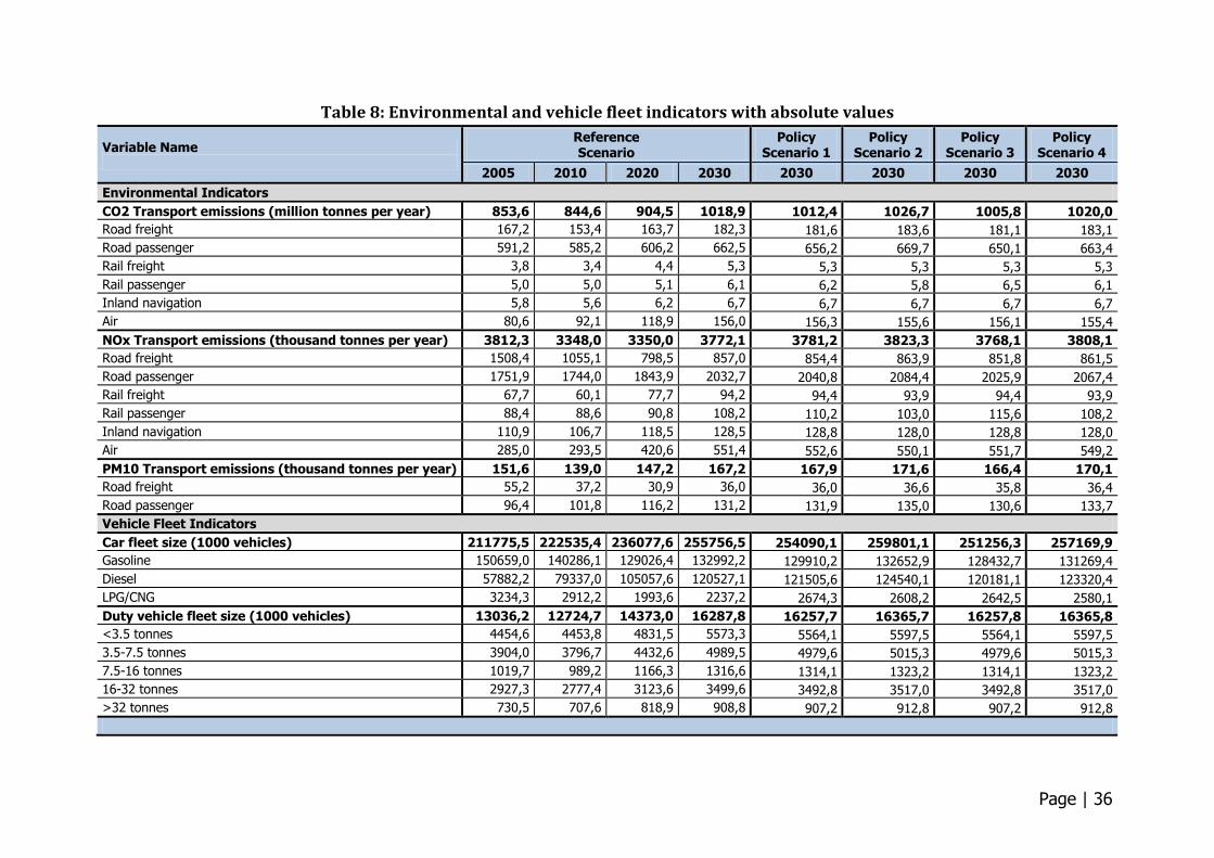
Page | 36

Table 8: Environmental and vehicle fleet indicators with absolute values

Variable Name

Reference Scenario

Policy Scenario 1

Policy Scenario 2

Policy Scenario 3

Policy Scenario 4

2005 2010 2020 2030 2030 2030 2030 2030

Environmental Indicators

CO2 Transport emissions (million tonnes per year) 853,6 844,6 904,5 1018,9 1012,4 1026,7 1005,8 1020,0

Road freight 167,2 153,4 163,7 182,3 181,6 183,6 181,1 183,1

Road passenger 591,2 585,2 606,2 662,5 656,2 669,7 650,1 663,4

Rail freight 3,8 3,4 4,4 5,3 5,3 5,3 5,3 5,3

Rail passenger 5,0 5,0 5,1 6,1 6,2 5,8 6,5 6,1

Inland navigation 5,8 5,6 6,2 6,7 6,7 6,7 6,7 6,7

Air 80,6 92,1 118,9 156,0 156,3 155,6 156,1 155,4

NOx Transport emissions (thousand tonnes per year) 3812,3 3348,0 3350,0 3772,1 3781,2 3823,3 3768,1 3808,1

Road freight 1508,4 1055,1 798,5 857,0 854,4 863,9 851,8 861,5

Road passenger 1751,9 1744,0 1843,9 2032,7 2040,8 2084,4 2025,9 2067,4

Rail freight 67,7 60,1 77,7 94,2 94,4 93,9 94,4 93,9

Rail passenger 88,4 88,6 90,8 108,2 110,2 103,0 115,6 108,2

Inland navigation 110,9 106,7 118,5 128,5 128,8 128,0 128,8 128,0

Air 285,0 293,5 420,6 551,4 552,6 550,1 551,7 549,2

PM10 Transport emissions (thousand tonnes per year) 151,6 139,0 147,2 167,2 167,9 171,6 166,4 170,1

Road freight 55,2 37,2 30,9 36,0 36,0 36,6 35,8 36,4

Road passenger 96,4 101,8 116,2 131,2 131,9 135,0 130,6 133,7

Vehicle Fleet Indicators

Car fleet size (1000 vehicles) 211775,5 222535,4 236077,6 255756,5 254090,1 259801,1 251256,3 257169,9

Gasoline 150659,0 140286,1 129026,4 132992,2 129910,2 132652,9 128432,7 131269,4

Diesel 57882,2 79337,0 105057,6 120527,1 121505,6 124540,1 120181,1 123320,4

LPG/CNG 3234,3 2912,2 1993,6 2237,2 2674,3 2608,2 2642,5 2580,1

Duty vehicle fleet size (1000 vehicles) 13036,2 12724,7 14373,0 16287,8 16257,7 16365,7 16257,8 16365,8

<3.5 tonnes 4454,6 4453,8 4831,5 5573,3 5564,1 5597,5 5564,1 5597,5

3.5-7.5 tonnes 3904,0 3796,7 4432,6 4989,5 4979,6 5015,3 4979,6 5015,3

7.5-16 tonnes 1019,7 989,2 1166,3 1316,6 1314,1 1323,2 1314,1 1323,2

16-32 tonnes 2927,3 2777,4 3123,6 3499,6 3492,8 3517,0 3492,8 3517,0

>32 tonnes 730,5 707,6 818,9 908,8 907,2 912,8 907,2 912,8

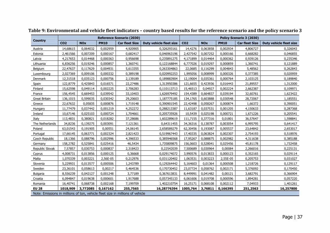
Page | 37

Table 9: Environmental and vehicle fleet indicators – country based results for the reference scenario and the policy scenario 3

Country Reference Scenario (2030) Policy Scenario 3 (2030)

CO2 NOx PM10 Car fleet Size Duty vehicle fleet size CO2 NOx PM10 Car fleet Size Duty vehicle fleet size

Austria 14,68615 0,064032 0,002959 4,920905 0,326293161 14,4276 0,063858 0,002934 4,806727 0,326043

Estonia 2,461566 0,007209 0,000167 0,682417 0,046963196 2,427542 0,007252 0,000166 0,668282 0,046855

Latvia 4,217653 0,014468 0,000363 0,956698 0,235891275 4,171899 0,014464 0,000362 0,939126 0,235346

Lithuania 6,836256 0,019246 0,000857 1,360741 0,122168844 6,777026 0,019297 0,000859 1,360741 0,121889

Belgium 22,47637 0,117629 0,004931 5,613355 0,263304863 22,0685 0,116299 0,004843 5,48562 0,262843

Luxembourg 2,027369 0,009106 0,000332 0,389198 0,020992253 1,995056 0,008999 0,000326 0,377385 0,020959

Denmark 12,31518 0,035123 0,000756 2,139189 0,189883904 12,19004 0,035361 0,000764 2,103125 0,189840

Spain 122,8779 0,425843 0,016571 22,27486 1,313950386 121,6655 0,423936 0,016443 21,89557 1,312000

Finland 15,62598 0,049114 0,002225 2,706283 0,110113713 15,46513 0,04927 0,002224 2,662387 0,109971

France 156,4545 0,669453 0,039542 33,10403 1,626979492 154,4389 0,664837 0,039194 32,60761 1,623422

Great Britain 136,1015 0,599035 0,030342 29,20603 1,187775185 134,1765 0,603888 0,030548 28,72067 1,185551

Greece 22,67632 0,05835 0,000876 1,719148 0,390901545 22,42498 0,058267 0,000874 1,66372 0,390051

Hungary 11,77479 0,037442 0,001219 4,252272 0,288213387 11,63187 0,037531 0,001205 4,150633 0,287368

Ireland 10,67146 0,025103 0,000724 1,704661 0,205735926 10,5439 0,025198 0,000721 1,671226 0,205541

Italy 113,4831 0,380821 0,018282 37,28686 1,602289619 111,7155 0,377316 0,01801 36,57647 1,598841

The Netherlands 34,8236 0,139275 0,003091 7,121361 0,64311455 34,36316 0,138787 0,003054 6,995795 0,641417

Poland 63,01543 0,191905 0,00551 24,06145 2,658589279 62,30456 0,193087 0,005537 23,64842 2,653017

Portugal 17,66145 0,063771 0,002324 2,821423 0,519967443 17,40335 0,063824 0,002307 2,754193 0,518976

Czech Republic 18,1366 0,088796 0,002996 4,396533 0,385946568 17,95267 0,088875 0,002982 4,311638 0,385188

Germany 158,2782 0,525841 0,025416 46,5434 1,735809875 156,0603 0,528041 0,025456 45,81178 1,732458

Republic Slovak 7,57857 0,030753 0,000837 2,318423 0,22542039 7,500689 0,030964 0,00084 2,266016 0,225131

Cyprus 4,008731 0,013856 0,000125 0,36668 0,029174072 3,990576 0,013833 0,000123 0,352165 0,029114

Malta 1,070339 0,003221 2,56E-05 0,212976 0,031120402 1,063531 0,003223 2,55E-05 0,205753 0,031027

Slovenia 5,229931 0,013577 0,000506 1,243789 0,129264442 5,164603 0,01364 0,000508 1,218726 0,129117

Sweden 23,36101 0,058613 0,00217 5,464536 0,170730452 23,07724 0,058762 0,002171 5,376092 0,170450

Bulgaria 8,556239 0,042127 0,001248 3,77189 0,367613831 8,449991 0,041482 0,00121 3,682791 0,366904

Croatia 6,094847 0,019638 0,000601 1,917688 0,057345133 6,061606 0,019708 0,000596 1,894281 0,057220

Romania 16,40741 0,068738 0,002168 7,199709 1,402210754 16,25171 0,068108 0,002112 7,04933 1,401261

EU 28 1018,909 3,772085 0,167162 255,7565 16,28776394 1005,764 3,76811 0,166395 251,2563 16,257800

Note: Emissions in millions of ton, vehicle fleet size in millions of vehicle

Page | 38

5.3. Evaluation of results and comparison of OPTIMISM policy

scenarios

Impacts on transport activity

The impacts on transport activity of the OPTIMISM policy scenarios are measured in

terms of changes in passenger kilometres for each mode of transport. A summary of

transport activity results for all scenarios with comparison to the 2030 reference

scenario are given in Table 10. Policy scenarios 3 and 4 included policy measures

that strongly supports co-modality and integration. In order to assess impacts of

OPTIMISM policy scenarios, at first the results for policy scenario 3, where

OPTIMISM strategies in an increasing fuel prices environment were implemented, are

compared with the reference scenario. According to the comparison of reference

scenario and policy scenario 3 the results indicate that:

Modal share for private cars decreases 1,7%, from 69,7% to 68,5%

Modal share for public road transport increases 8,3%, from 7,7% to 8,4

Modal share for rail transport increases 6.9%, from 9,3% to 10,0%.

In addition to this,

Travel per person by public road transport and rail increases by 7,5%,

Travel per person by private cars and motorcycles decreases by 1,7%.

Apart from this, it is also important to see the potential impacts of OPTIMISM policy

measures and fuel prices separately. In order to better understand the impact of

OPTIMISM strategies solely, a comparison between policy scenarios 1 and 3 is

required. In this way the impact of fuel prices (fuel prices are increasing in both of

these scenarios) can be removed from the results. With this respect, according to the

comparison of policy scenario 1 and 3:

Modal share for private cars decreases 1,3%, from 69,4% to 68,5%

Modal share for public road transport increases 7,7%, from 7,8% to 8,4%

Modal share for public road transport increases 5,2%, from 9,5% to 10,0%


Travel per person by public road transport and rail increases by 5.9% from

2598 to 2750 (km per capita)

Travel per person by private cars and motorcycles decreases by 1,1% from


Page | 39

Table 10: OPTIMISM transport activity estimations for 2030: comparison of scenarios by transport mode

EU 28 2010

2030 Reference Scenario

2030 Policy Scenario 1




Value Rate Value Rate Value Rate Change Value Rate Change Value Rate Change Value Rate Change

Passenger transport activity (Gkms)

6418.9 100% 7902.3 100% 7889.6 100% -.16% 7939.1 100% 0.47% 7905.9 100% 0.05% 7930.2 100% 0.35%

Public road transport 513.5 8.0% 610.6 7.7% 618.3 7.8% 1.27% 593.4 7.5% -2.82% 661.3 8.4% 8.31% 610.6 7.7% 0.00%

Private cars 4763.3 74.2% 5509.34 69.7% 5473.4 69.4% -0.65% 5596.1 70.5% 1.58% 5413.9 68.5% -1.73% 5540.6 69.9% 0.57%

Motorcycles 120.3 1.9% 153.94 1.9% 153.0 1.9% -0.64% 156.3 2.0% 1.51% 150.9 1.9% -1.96% 154.5 1.9% 0.34%

Rail 496.2 7.7% 735.8 9.3% 750.3 9.5% 1.97% 703.1 8.9% -4.44% 786.9 10.0% 6.94% 735.8 9.3% 0.00%

Aviation 525.6 8.2% 892.6 11.3% 894.6 11.3% 0.23% 890.2 11.2% -0.27% 893.0 11.3% 0.04% 888.7 11.2% -0.44%

Freight transport activity (Gtkm)

2306.1 100% 3008.8 100% 3005.7 100% -.10% 3017.4 100% 0.29% 3005.7 100% -.10% 3017.4 100% 0.29%

Trucks 1764.4 76.5% 2245.83 74.6% 2241.4 74.6% -0.20% 2256.9 74.8% 0.49% 2241.5 74.6% -0.19% 2256.9 74.8% 0.49%

Rail 392.5 17.0% 583.63 19.4% 584.5 19.4% 0.14% 581.9 19.3% -0.29% 584.5 19.4% 0.14% 581.9 19.3% -0.29%

Inland water ways 149.2 6.5% 179.3 6.0% 179.8 6.0% 0.26% 178.6 5.9% -0.40% 179.8 6.0% 0.26% 178.6 5.9% -0.40%

Activity indicators

Travel per person (km per capita) 12701 15003 14979 -0.16% 15073 0.47% 15010 0.05% 15056 0.35%


9663 10752 10682 -0.65% 10922 1.57% 10565 -1.74% 10813 0.56%


1998 2556 2598 1.65% 2461 -3.71% 2750 7.56% 2556 0.00%


187 181 180 -0.10% 181 0.29% 180 -0.10% 181 0.29%

GDP (in 000 Meuro`10) 12301.9 16667.6 --- --- --- --- --- --- --- ---

Population (Million) 505.4 526.7 --- --- --- --- --- --- --- ---



Policy Scenario 1 with increasing (high) fuel prices and internalization of external costs for road transport Policy Scenario 2 with not increasing (low) fuel prices



Note: Change column indicates the difference between the policy scenario and the reference scenario in percentages.

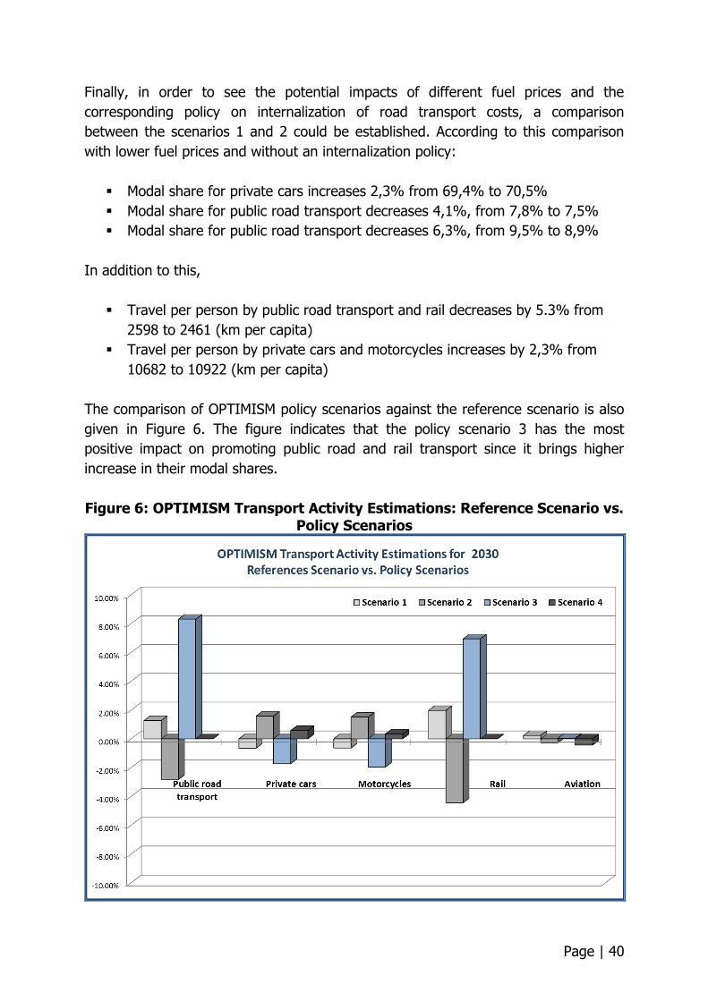
Page | 40

Finally, in order to see the potential impacts of different fuel prices and the

corresponding policy on internalization of road transport costs, a comparison

between the scenarios 1 and 2 could be established. According to this comparison

with lower fuel prices and without an internalization policy:

Modal share for private cars increases 2,3% from 69,4% to 70,5%

Modal share for public road transport decreases 4,1%, from 7,8% to 7,5%

Modal share for public road transport decreases 6,3%, from 9,5% to 8,9%


Travel per person by public road transport and rail decreases by 5.3% from


Travel per person by private cars and motorcycles increases by 2,3% from


The comparison of OPTIMISM policy scenarios against the reference scenario is also

given in Figure 6. The figure indicates that the policy scenario 3 has the most

positive impact on promoting public road and rail transport since it brings higher

increase in their modal shares.

Figure 6: OPTIMISM Transport Activity Estimations: Reference Scenario vs. Policy Scenarios

Page | 41

Today, the share of private cars in passenger transport is 74% and it is expected to

reduce up to 70% by 2030. It is also expected that the mode share of rail transport

will increase from 7,7% to 9,3% and aviation from 8,2% to 11,3% by 2030 (Table

10). The results of the simulations show that the OPTIMISM policy measures may

have significant impacts on this existing trend in passenger transport activity.

No significant change in total transport demand is foreseen with the implementation

of OPTIMISM policy scenarios. However, it is obvious that the selected policy

measures will increase public transport share both for the road and rail transport and

decrease the share of private cars and motorcycles in total passenger kilometres.

Considering the potential impacts of the OPTIMISM policy measures without the

impact of fuel prices (comparison of policy scenarios 1 and 3), average travel per

person by public road transport and rail increases by 5.9% and travel per person by

private cars and motorcycles decreases by 1,1%.

Environmental impacts

Environmental impacts of the OPTIMISM policy scenarios are estimated using

TREMOVE System Dynamics. The environmental impacts for all scenarios with

comparison to the 2030 reference scenario are given in Table 11. The tables include

the CO2, NOx and PM10 transport emissions as well as the vehicle fleet sizes. The

policy scenarios 3 and 4 include OPTIMISM strategies and policy measures that

strongly support co-modality and integration. In order to assess the impact of

OPTIMISM strategies, at first the results for policy scenario 3 are highlighted; in this

scenario the OPTIMISM policy measures are implemented in an increasing fuel prices

environment with an internalization policy. According to the comparison of reference

scenario and policy scenario 3 the results indicate:

CO2 transport emissions decreases by 1.3% in total and 1.9% for road

passenger transport, from 1018 to 1005 and from 662 to 650 (million tons per

year),

NOx transport emissions decreases by 0.1% in total and decreases 0.3% for

road passenger transport, from 3772 to 3768 and from 2032 to 2025

(thousand tons per year),

PM10 transport emissions decreases by 0.5% in total and decreases 0.5% for

road passenger transport, from 167.2 to 166.4 and from 131.2 to 130.6

(thousand tons per year),

Car fleet size decreases from 255 million to 251 million with 1.8% change and

number of cars with LPG/CNG technology increases by 18.2%, from 2.2

million to 2.6 million.

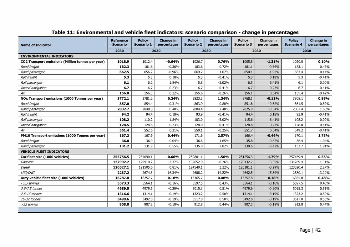
Page | 42

Table 11: Environmental and vehicle fleet indicators: scenario comparison - change in percentages

Name of Indicator

Reference Scenario

Policy Scenario 1

Change in percentages

Policy Scenario 2


Policy Scenario 3


Policy Scenario 4


2030 2030 2030 2030 2030

ENVIRONMENTAL INDICATORS

CO2 Transport emissions (Million tonnes per year) 1018.9 1012.4 -0.64% 1026.7 0.76% 1005.8 -1.31% 1020.0 0.10%

Road freight 182.3 181.6 -0.36% 183.6 0.72% 181.1 -0.66% 183.1 0.45%

Road passenger 662.5 656.2 -0.96% 669.7 1.07% 650.1 -1.92% 663.4 0.14%

Rail freight 5.3 5.3 0.18% 5.3 -0.41% 5.3 0.18% 5.3 -0.41%

Rail passenger 6.1 6.2 1.84% 5.8 -5.02% 6.5 6.41% 6.1 0.00%

Inland navigation 6.7 6.7 0.23% 6.7 -0.41% 6.7 0.23% 6.7 -0.41%

Air 156.0 156.3 0.22% 155.6 -0.26% 156.1 0.04% 155.4 -0.42%

NOx Transport emissions (1000 Tonnes per year) 3772.1 3781.2 0.24% 3823.3 1.34% 3768.1 -0.11% 3808.1 0.95%

Road freight 857.0 854.4 -0.31% 863.9 0.80% 851.8 -0.62% 861.5 0.52%

Road passenger 2032.7 2040.8 0.40% 2084.4 2.48% 2025.9 -0.34% 2067.4 1.68%

Rail freight 94.2 94.4 0.18% 93.9 -0.41% 94.4 0.18% 93.9 -0.41%

Rail passenger 108.2 110.2 1.84% 103.0 -5.02% 115.6 6.41% 108.2 0.00%

Inland navigation 128.5 128.8 0.23% 128.0 -0.41% 128.8 0.23% 128.0 -0.41%

Air 551.4 552.6 0.21% 550.1 -0.25% 551.7 0.04% 549.2 -0.41%

PM10 Transport emissions (1000 Tonnes per year) 167.2 167.9 0.44% 171.6 2.57% 166.4 -0.46% 170.1 1.73%

Road freight 36.0 36.0 0.04% 36.6 1.65% 35.8 -0.62% 36.4 1.04%

Road passenger 131.2 131.9 0.55% 135.0 2.82% 130.6 -0.42% 133.7 1.91%

VEHICLE FLEET INDICATORS

Car fleet size (1000 vehicles) 255756.5 254090.1 -0.66% 259801.1 1.56% 251256.3 -1.79% 257169.9 0.55%

Gasoline 132992.2 129910.2 -2.37% 132652.9 -0.26% 128432.7 -3.55% 131269.4 -1.31%

Diesel 120527.1 121505.6 0.81% 124540.1 3.22% 120181.1 -0.29% 123320.4 2.27%

LPG/CNG 2237.2 2674.3 16.34% 2608.2 14.22% 2642.5 15.34% 2580.1 13.29%

Duty vehicle fleet size (1000 vehicles) 16287.8 16257.7 -0.18% 16365.7 0.48% 16257.8 -0.18% 16365.8 0.48%

<3.5 tonnes 5573.3 5564.1 -0.16% 5597.5 0.43% 5564.1 -0.16% 5597.5 0.43%

3.5-7.5 tonnes 4989.5 4979.6 -0.20% 5015.3 0.51% 4979.6 -0.20% 5015.3 0.51%

7.5-16 tonnes 1316.6 1314.1 -0.19% 1323.2 0.50% 1314.1 -0.19% 1323.2 0.50%

16-32 tonnes 3499.6 3492.8 -0.19% 3517.0 0.50% 3492.8 -0.19% 3517.0 0.50%

>32 tonnes 908.8 907.2 -0.18% 912.8 0.44% 907.2 -0.18% 912.8 0.44%

Page | 43

In addition to this, if we compare the policy scenarios 1 and 3 to remove the impact

of fuel prices and to see the impact of OPTIMISM strategies solely, the results

indicate:

CO2 transport emissions decreases by 0.7% in total and 0.9% for road

passenger transport,

NOx transport emissions decreases by 0.3% in total and decreases 0.7% for

road passenger transport,

PM10 transport emissions decreases by 0.9% in total and decreases 1.0% for

road passenger transport,

Car fleet size decreases from 254 million to 251 million with 1.1% change.

Several other elements of conclusion can be mentioned as well:

Increase in fuel prices in order to capture the impact of internalization

measures can reduce the total EU-28 truck transport activity by around 0.20%

in 2030 as shown by scenarios 1 and 3. Results of both scenarios show

decrease of around 0.19% in heavy duty vehicle fleet size in all categories.

CO2, NOX and PM10 emissions from road freight transport decrease from

0.3% to 0.6% in both scenarios.

Scenario 2 that represents low fuel price situation combined with no measures

of co-modality appears to be the worst scenario in term of emissions in

comparison to the reference scenario. In 2030 we can expect that CO2, NOX

and PM10 emission will increase by 0.77%, 1.36% and 2.36% respectively.

Implementation of co-modality measures through reduction of transport costs

in tram, buses and metro only as simulated in the scenario 4 will could slightly

improve the situation in comparison to the scenario 2. However emissions of

CO2, NOX and PM10 will still increase by 2030 by 0.11%, 0.95% and 1.73%

respectively with regards to reference scenario.

Considering the reference scenario for 2030, transport emissions will keep increasing

and the road passenger transport will be responsible for 65% of the total CO2

transport emissions and 54% of the total NOx transport emissions (Table 11). The

modelling exercise indicates that to counter this trend is not an easy task. With the

best policy scenario including strategies to support co-modality and integration, only

slight differences can be achieved in the transport emissions. The reduction in the

transport emissions is approximately 1%.

Page | 44

Slight impacts of the scenarios in term of emissions changes could be explained first

by the fact that scenario measures only have limited impact on changes in transport

activities of the principal emitters, i.e. trucks and private cars. For example in 2030,

changes of transport activities in private cars range only between -1.73 and 1.58% in

the four scenarios. These values are even smaller for trucks, i.e. from -0.20% to

.49% in the four scenarios since the OPTIMISM strategies focus on passenger

transport. Second, as no technological measure is involved all strategies of the

different scenarios only affect energy use and emission indirectly, i.e. through

changes in generalized costs that induce user to choose more energy efficient vehicle

types. The limitations of the modelling exercise - such as lack of proper transfer of

policies into aviation sector or into urban transport - could be the other reason. The

results show that implementing the OPTIMISM strategy has positive environmental

impacts, but they are not, on their own, sufficient to reach EU targets for reducing

transport emissions.

Page | 45

6. Concluding remarks

OPTIMISM proposed five strategies aiming to optimize passenger transport system to

promote public transport and to support co-modality and integration: a) seamless

international travel, b) seamless regional/national travel, c) integrated urban and

metropolitan transport, d) integrated and personalised information, and e) new

mobility paradigm based on public means of transport both individual and collective.

The main objectives when proposing these strategies have been:

to increase public transport share,

to improve co-modal transport activities,

to improve ease of travel with better travel information services, integrated

ticketing, and improved transport management,

to reduce congestion and GHG emissions,

to improve border-crossings and interchange points,

to achieve more efficient usage of transport infrastructure and services

The strategies consist of a common subset of co-modality and integration measures

selected from a set of broader list. The selected policy measures for the scenario

simulation which are mainly ICT-based measures are:

Provision of travel Information

Integrated ticket and innovative ticketing

Improvement of luggage transport and passenger check-in

Innovative local mobility services

Improvement of mobility service at local level

Improvements at interchange points

Transport system infrastructure and rolling-stock improvements

One of the first objective of macro simulation for passenger transport in this

deliverable was to estimate potential mobility and environmental impacts of these

selected policy measures. Therefore, "support of sustainable transport policies" was

defined as the first scenario variable. The other identified scenario variable was

"energy prices" which may follow two possible trends according to the project: the

first is the baseline trend (increasing) the second is the global action trend (not

increasing) for oil prices. According to the these two drivers, four policy scenarios

were designed as well as a reference scenario for 2030:

Reference Scenario: with increasing (high) fuel prices,

Policy Scenario 1: with increasing (high) fuel prices and internalization of

external costs for road transport,

Page | 46

Policy Scenario 2: with not increasing (low) fuel prices,

Policy Scenario 3 (sustainable 1): with increasing (high) fuel prices and

internalization of external costs for road transport & sustainable policies for

promoting public transport and supporting co-modality and integration.

Policy Scenario 4 (sustainable 2): with not increasing (low) fuel prices &

sustainable policies for promoting public transport and supporting co-modality

and integration.

The transport activity indicators for each of the policy scenarios were estimated with

TRANS-TOOLS-S Demand Module (TDM), then these estimations on transport

demand fed into the TREMOVE System Dynamics (TSD) to estimate environmental

impacts of the policy scenarios. At the end, the policy scenarios and the reference

scenario were compared between each other to explore the potential impacts of

different trends in fuel prices and implementation of OPTIMISM policy measures.

Based on the results of scenario simulations, the following elements of conclusion

has to be underlined.

a) As of 2010, the share of private cars in passenger transport is 74% and it is

expected to reduce up to 70% by 2030. It is also expected that the mode share of

rail transport will increase from 7,7% to 9,3% and aviation from 8,2% to 11,3% by

2030. The results of the simulations show that the OPTIMISM policy measures may

have significant impacts on existing mobility pattern through a substantial modal shift

from private car to public transport. More specifically, with the implementation of

OPTIMISM strategies/policy measures in an increasing fuel prices environment:

The modal share of private cars may decrease by 1,7% where modal share for

public road transport and rail transport may increase by 8,3% and 6.9%

respectively,

Travel per person by private cars and motorcycles may decrease by 1,7%

where travel per person by public road transport and rail is increasing by

7,5%.

b) No significant change in total transport demand is foreseen with the

implementation of OPTIMISM policy scenarios. However, it is obvious that the

selected policy measures will increase public transport share both for the road and

rail transport and decrease the share of private cars and motorcycles. Considering

the potential impacts of the OPTIMISM policy measures without the impact of fuel

prices (comparison of policy scenarios 1 and 3), travel per person by public road

transport and rail increases by 5.9% and travel per person by private cars and

motorcycles decreases by 1,1%.

Page | 47

c) According to the reference scenario for 2030, transport emissions will keep

increasing and the road passenger transport will be responsible for 65% of the total

CO2 transport emissions and 54% of the total NOx transport emissions. The

modelling exercise indicates that it is very difficult to shift this trend. With the best

policy scenario including strategies to support co-modality and integration, only slight

differences can be achieved in the transport emissions.

d) However, the modal shift from passenger cars to public road and rail

transport may still result in positive environmental impacts. Combination of

OPTIMISM co-modality and internalisation measures represented in the policy

scenario 3 may reduce the CO2, NOx and PM10 transport emissions in 2030 by

1.3%, 0.1% and 0.4% respectively mainly through fall in road transport emissions.

e) Different trends in fuel prices may also have important impacts on mobility

pattern. Lower fuel prices without any policy on internalization of road transport

costs have significant negative impacts on reducing share of private cars in total

transport activity. With lower fuel prices and without an internalization policy, travel

per person by public road transport and rail may decrease by 5.3% while travel per

person by private cars and motorcycles is increasing by 2,3%.

In conclusion, OPTIMISM strategies/policy measures to support co-modality and

integration have positive mobility and environmental impacts. These positive impacts

are more noticeable particularly in higher fuel prices environment and with

internalization of external costs of road transport. The results show that

implementing the OPTIMISM strategies has positive environmental impacts, but they

are not, on their own, sufficient to reach EU targets for reducing transport emissions.

Since the OPTIMISM scenarios mainly simulated impacts of two specific variables -

fuel prices and co-modality strategies - and it was mainly compared with the

reference scenario for 2030 which already includes several strategies in the same

direction, only slight differences in the environmental impacts have been observed.

Apart from this, the OPTIMISM strategies mainly comprise ICT-based policy

measures and for only passenger transport excluding the freight transport, hence

their impact on transport emissions is rather small. Finally, the OPTIMISM strategies

aiming to support co-modal and integrated passenger transport should be supported

by other policies in vehicle and fuel technologies and with infrastructure

improvements, road charging, taxation and traffic restriction policies in order to be

able to achieve better solutions for sustainable passenger transport.

Page | 48

References

Akkermans, L. and Maerivoet, S., (2013), "Impacts of best practices on mobility

patterns", Project Deliverable 4.2, OPTIMISM: Optimising Passenger Transport

Information to Materialize Insights for Sustainable Mobility, FP7 – 284892.

AMITRAN Consortium, (2013), "Methodology for classification of ITS", Project

Deliverable 3.1, AMITRAN Project: CO2 Assessment Methodology for ICT in

Transport, FP7 – 287551.

Christidis P., Nemry F., Ibañez N. and Navajas E., (2010), "Transport demand

projections until 2030 - Reference scenario". JRC Technical notes, European

Commission, Joint Research Centre, Ins. for Pros. Tech. Studies.

De Ceuster, G., van Herbruggen, B., Ivanova, O., Carlier, K., Martino, A. and Fiorello,

D., (2007), "TREMOVE: service contract for the further development and

application of the transport and environmental TREMOVE model", Final

Report, Transport & Mobility Leuven, Leuven, Belgium.

Delle Site, P., Filippi, F. and Salucci, M.V., (2013a), "Delphi expert report on the

future scenarios of transport and mobility", Deliverable 3.3: OPTIMISM

Project: Optimising Passenger Transport Information to Materialize Insights

for Sustainable Mobility, FP7 - 284892.

Delle Site, P., Filippi, F., Salucci, M.V., Zhang, Q., Brooks, R., Micharikopoulos, D.,

Tavlaki, E., Kompil, M., Hoppe, M., Seppänen, T. and Christ, A., (2013b),

"Definition of strategies for integrating and optimising transport systems",

Deliverable 5.1: OPTIMISM Project: Optimising Passenger Transport

Information to Materialize Insights for Sustainable Mobility, FP7 - 284892.

Delle Site, P., Salucci, M. V., Hoppe, M., Seppänen, T., Christ, A., Arsenio, E., van

Grinsven, A., Morris, D., Anoyrkati, E., Brooks, R., Hepting, M., Kompil, M.,

Tavlaki, E., Micharikopoulos, D. and Akkermans L., (2012), "List of potential

megatrends influencing transport system and mobility behaviour", Project

Deliverable 3.2, OPTIMISM: Optimising Passenger Transport Information to

Materialize Insights for Sustainable Mobility, FP7 - 284892.

European Commission, (2011a), " Impact Assessment - White Paper: Roadmap to a

Single European Transport Area - Towards a competitive and resource

efficient transport system, SEC (2011) 358 final, Brussels.

European Commission, (2011b), "Impact Assessment - A Roadmap for moving to a

competitive low carbon economy in 2050", SEC (2011) 288 final, Brussels.

European Commission, (2012), "2012 EU Reference Scenario modelling - Draft

transport activity projections", Directorate General Energy, Directorate General

Climate Action, Directorate General Mobility and Transport.

Fiorello, D., De Stasio, C., Köhler, J., Kraft, M., Newton, S., Purwanto, J., Schade, B.,

Schade, W., Szimba, E., (2009) "The iTREN-2030 reference scenario until

2030", Deliverable 4 of iTREN-2030 (Integrated transport and energy baseline

until 2030), European Commission 6th RTD Programme, Milan, Italy.

Page | 49

Hansen, S., (2011a), TRANS-TOOLS Implementing Scenarios, Project: TRANS-TOOLS

v2.0 Documentation, Rapidis, Denmark.

Hansen, S., (2011b), TRANS-TOOLS User Guide, Project: TRANS-TOOLS v2.0

Documentation, Rapidis, Denmark.

Hidalgo, I., Purwanto, J., Vanherle, K., Fermi, F. and Fiorello, D. (2011), "GLADYSTE:

Transposing the structure of the TREMOVE model into a system dynamics

coding", Final Report, J02/32/2008, Transport & Mobility Leuven, Belgium.

Hoppe, M., Delle Site, P., Salucci, M. V., Hepting, M., Arsenio, E., Kompil, M. and

Anoyrkati, E., (2012), "Research Scheme for Transport System and Mobility

Behaviour", Project Deliverable 3.1, OPTIMISM: Optimising Passenger

Transport Information to Materialize Insights for Sustainable Mobility,

FP7 - 284892.

Lopez-Ruiz H. G., Christidis P., Demirel H. and Kompil M., 2013, "Quantifying the

Effects of Sustainable Urban Mobility Plans", JRC Technical Reports, ISBN:

978-9279-3272-1, DOI: 10.279/21875, Luxembourg.

OPTIMISM Consortium, (2012), "Identification of ICT options enhancing co-

modality", Project Deliverable 4.1, OPTIMISM: Optimising Passenger Transport

Information to Materialize Insights for Sustainable Mobility, FP7 – 284892,

main author: CE Delft.

Schade, W. and Krail, M., (2010), "iTREN-2030: Experiences and results for

integrated technology, energy and transport policy assessment", Final Report

and Deliverable 6 of iTREN-2030 (Integrated transport and energy baseline

until 2030), Project co-funded by European Commission 6th RTD Programme,

Fraunhofer-ISI, Karlsruhe, Germany.

TNO, (2006), "Review and analysis of the reduction potential and costs of

technological and other measures to reduce CO2 emissions from passenger

cars", Final report to the European Commission, Contract no SI2.408212.

Transport & Mobility Leuven, (2007), "TREMOVE model description",

http://www.tremove.org/documentation/TREMOVE_Short_Description.pdf –

access date 25.09.2013.

TRANS-TOOLS, (2008a), TRANS-TOOLS Documentation, EC, JRC, Institute for

Prospective for Prospective Technological Studies,

http://energy.jrc.ec.europa.eu/transtools/documentation.html – access date

25.09.2013.

TRANS-TOOLS, (2008b), TRANS-TOOLS Home, EC, JRC, Institute for Prospective

Technological Studies, http://energy.jrc.ec.europa.eu/transtools/index.html –

access date 25.09.2013.

Vannacci, L., Condeco, A., Lopez, H., Demirel, H., Ibanez N., Navajas, E. and

Christidis, P., (2013), "TRANSTOOLS-S: A comprehensive approach for an EU

transport network model", Draft Interim Report, JRC Scientific and Policy

Reports, European Commission, Joint Research Centre, Institute for

Prospective Technological Studies.

http://www.tremove.org/documentation/TREMOVE_Short_Description.pdf

http://energy.jrc.ec.europa.eu/transtools/documentation.html

http://energy.jrc.ec.europa.eu/transtools/index.html

Page | 50

Appendix

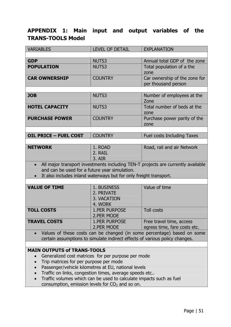
Page | 51

APPENDIX 1: Main input and output variables of the

TRANS-TOOLS Model

VARIABLES LEVEL OF DETAIL EXPLANATION

GDP NUTS3 Annual total GDP of the zone

POPULATION NUTS3 Total population of a the zone

CAR OWNERSHIP COUNTRY Car ownership of the zone for per thousand person

JOB NUTS3 Number of employees at the Zone

HOTEL CAPACITY NUTS3 Total number of beds at the zone

PURCHASE POWER COUNTRY Purchase power parity of the zone

OIL PRICE – FUEL COST COUNTRY Fuel costs Including Taxes

NETWORK 1. ROAD 2. RAIL 3. AIR

Road, rail and air Network

All major transport investments including TEN-T projects are currently available and can be used for a future year simulation.

It also includes inland waterways but for only freight transport.

VALUE OF TIME 1. BUSINESS 2. PRIVATE 3. VACATION 4. WORK

Value of time

TOLL COSTS 1.PER PURPOSE 2.PER MODE

Toll costs

TRAVEL COSTS 1.PER PURPOSE 2.PER MODE

Free travel time, access egress time, fare costs etc.

Values of these costs can be changed (in some percentage) based on some certain assumptions to simulate indirect effects of various policy changes.

MAIN OUTPUTS of TRANS-TOOLS Generalized cost matrices for per purpose per mode

Trip matrices for per purpose per mode Passenger/vehicle kilometres at EU, national levels Traffic on links, congestion times, average speeds etc.. Traffic volumes which can be used to calculate impacts such as fuel

consumption, emission levels for CO2 and so on.

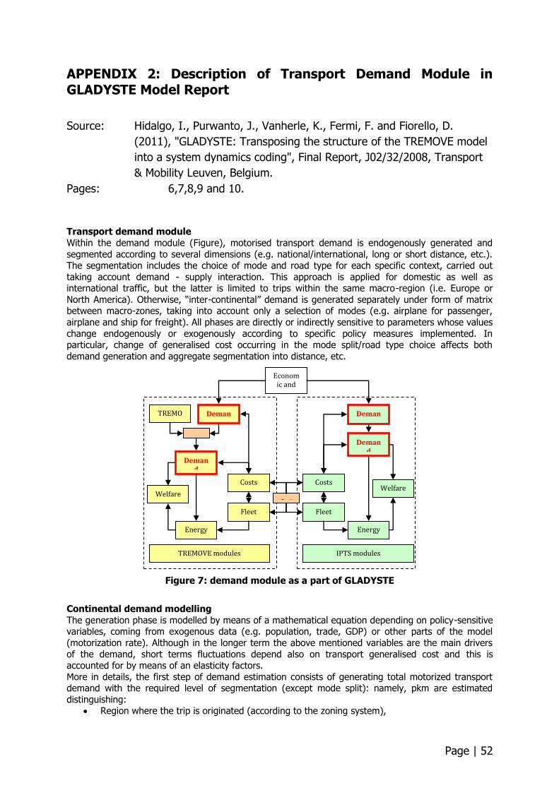
Page | 52

APPENDIX 2: Description of Transport Demand Module in GLADYSTE Model Report

Source: Hidalgo, I., Purwanto, J., Vanherle, K., Fermi, F. and Fiorello, D.

(2011), "GLADYSTE: Transposing the structure of the TREMOVE model

into a system dynamics coding", Final Report, J02/32/2008, Transport

& Mobility Leuven, Belgium.

Pages: 6,7,8,9 and 10.

Transport demand module

Within the demand module (Figure), motorised transport demand is endogenously generated and

segmented according to several dimensions (e.g. national/international, long or short distance, etc.). The segmentation includes the choice of mode and road type for each specific context, carried out

taking account demand - supply interaction. This approach is applied for domestic as well as international traffic, but the latter is limited to trips within the same macro-region (i.e. Europe or

North America). Otherwise, “inter-continental” demand is generated separately under form of matrix between macro-zones, taking into account only a selection of modes (e.g. airplane for passenger,

airplane and ship for freight). All phases are directly or indirectly sensitive to parameters whose values

change endogenously or exogenously according to specific policy measures implemented. In particular, change of generalised cost occurring in the mode split/road type choice affects both

demand generation and aggregate segmentation into distance, etc.

Figure 7: demand module as a part of GLADYSTE

Continental demand modelling

The generation phase is modelled by means of a mathematical equation depending on policy-sensitive variables, coming from exogenous data (e.g. population, trade, GDP) or other parts of the model

(motorization rate). Although in the longer term the above mentioned variables are the main drivers

of the demand, short terms fluctuations depend also on transport generalised cost and this is accounted for by means of an elasticity factors.

More in details, the first step of demand estimation consists of generating total motorized transport demand with the required level of segmentation (except mode split): namely, pkm are estimated

distinguishing: Region where the trip is originated (according to the zoning system),

TREMOVE modules (EU31)

IPTS modules (EU31 AND ROW)

Economic and

demographic inputs Deman

d genera

tion

TREMOVE

demand input

Demand

segmentation

Costs

Fleet plannin

g Energy and

emissions

Welfare

Switch

Switch

Demand

generation Deman

d segme

ntation

Costs

Fleet plannin

g

Welfare

Energy and

emissions

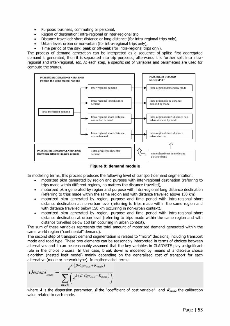
Page | 53

Purpose: business, commuting or personal,

Region of destination: intra-regional or inter-regional trip,

Distance travelled: short distance or long distance (for intra-regional trips only),

Urban level: urban or non-urban (for intra-regional trips only),

Time period of the day: peak or off-peak (for intra-regional trips only).

The process of demand generation can be interpreted as a sequence of splits: first aggregated demand is generated, then it is separated into trip purposes, afterwards it is further split into intra-

regional and inter-regional, etc. At each step, a specific set of variables and parameters are used for

compute the shares.

Figure 8: demand module

In modelling terms, this process produces the following level of transport demand segmentation: motorized pkm generated by region and purpose with inter-regional destination (referring to

trips made within different regions, no matters the distance travelled),

motorized pkm generated by region and purpose with intra-regional long distance destination

(referring to trips made within the same region and with distance travelled above 150 km), motorized pkm generated by region, purpose and time period with intra-regional short

distance destination at non-urban level (referring to trips made within the same region and

with distance travelled below 150 km occurring in non-urban context), motorized pkm generated by region, purpose and time period with intra-regional short

distance destination at urban level (referring to trips made within the same region and with

distance travelled below 150 km occurring in urban context),

The sum of these variables represents the total amount of motorized demand generated within the same world region (“continental” demand).

The second step of transport demand segmentation is related to “micro” decisions, including transport mode and road type. These two elements can be reasonably interpreted in terms of choices between

alternatives and it can be reasonably assumed that the key variables in GLADYSTE play a significant

role in the choice process. In this case, break down is modelled by means of a discrete choice algorithm (nested logit model) mainly depending on the generalised cost of transport for each

alternative (mode or network type). In mathematical terms:

mode

mode

K

K

mode

mode

mode

Cgen

mode CgenDemand

e=

e

where λ is the dispersion parameter, β the “coefficient of cost variable” and Kmode the calibration

value related to each mode.

Total motorized demand

Inter-regional demand

Intra-regional long distance demand

Intra-regional short-distance non-urban demand

Intra-regional short-distance urban demand

Inter-regional demand by mode

Intra-regional long distance demand by mode

Intra-regional short-distance non-urban demand by mode

Intra-regional short-distance urban demand

Generalised cost by mode and distance band

PASSENGER DEMAND GENERATION (within the same macro-region)

PASSENGER DEMAND MODE SPLIT

Total air intercontinental demand

PASSENGER DEMAND GENERATION (between different macro-regions)

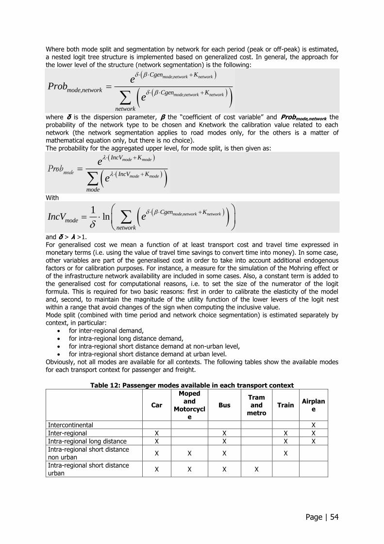
Page | 54

Where both mode split and segmentation by network for each period (peak or off-peak) is estimated, a nested logit tree structure is implemented based on generalized cost. In general, the approach for

the lower level of the structure (network segmentation) is the following:

mode,network network

mode,network network

Cgen K

mode,network Cgen K

network

Probe

e

where δ is the dispersion parameter, β the “coefficient of cost variable” and Probmode,network the probability of the network type to be chosen and Knetwork the calibration value related to each

network (the network segmentation applies to road modes only, for the others is a matter of mathematical equation only, but there is no choice).

The probability for the aggregated upper level, for mode split, is then given as:

mode mode

mode mode

IncV K

IncV K

mode

e

e

modeProb

With

ln1

mode,network networkCgen K

mode

network

IncV e

and δ > λ >1. For generalised cost we mean a function of at least transport cost and travel time expressed in

monetary terms (i.e. using the value of travel time savings to convert time into money). In some case,

other variables are part of the generalised cost in order to take into account additional endogenous factors or for calibration purposes. For instance, a measure for the simulation of the Mohring effect or

of the infrastructure network availability are included in some cases. Also, a constant term is added to the generalised cost for computational reasons, i.e. to set the size of the numerator of the logit

formula. This is required for two basic reasons: first in order to calibrate the elasticity of the model

and, second, to maintain the magnitude of the utility function of the lower levers of the logit nest within a range that avoid changes of the sign when computing the inclusive value.

Mode split (combined with time period and network choice segmentation) is estimated separately by context, in particular:

for inter-regional demand,

for intra-regional long distance demand,

for intra-regional short distance demand at non-urban level,

for intra-regional short distance demand at urban level.

Obviously, not all modes are available for all contexts. The following tables show the available modes for each transport context for passenger and freight.

Table 12: Passenger modes available in each transport context

Car

Moped

and

Motorcycle

Bus Tram and

metro

Train Airplan

e

Intercontinental X

Inter-regional X X X X

Intra-regional long distance X X X X

Intra-regional short distance

non urban X X X X


urban X X X X

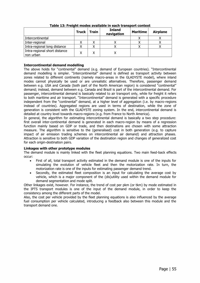
Page | 55

Table 13: Freight modes available in each transport context

Truck Train Inland

navigation Maritime Airplane

Intercontinental X X

Inter-regional X X X X X

Intra-regional long distance X X X X X


non urban X X X

Intercontinental demand modelling

The above holds for “continental” demand (e.g. demand of European countries). “Intercontinental demand modelling is simpler. “Intercontinental” demand is defined as transport activity between

zones related to different continents (namely macro-areas in the GLADYSTE model), where inland modes cannot physically be used or are unrealistic alternatives. Therefore, passenger demand

between e.g. USA and Canada (both part of the North American region) is considered “continental”

demand; instead, demand between e.g. Canada and Brazil is part of the intercontinental demand. For passenger, intercontinental demand is basically related to air transport only, while for freight it refers

to both maritime and air transport. “Intercontinental” demand is generated with a specific procedure independent from the “continental” demand, at a higher level of aggregation (i.e. by macro-regions

instead of countries). Aggregated regions are used in terms of destination, while the zone of

generation is consistent with the GLADYSTE zoning system. In the end, intercontinental demand is detailed at country level towards macro-regions (e.g. from France to North America).

In general, the algorithm for estimating intercontinental demand is basically a two step procedure: first overall inter-continental demand is generated in each macro-region by means of a regression

function mainly based on GDP or trade, and then destinations are chosen with some attraction measure. The algorithm is sensitive to the (generalised) cost in both generation (e.g. to capture

impact of air emission trading schemes on intercontinental air demand) and attraction phases.

Attraction is sensitive to both GDP variation of the destination region and changes of generalized cost for each origin-destination pairs.

Linkages with other prototype modules The demand module is mainly linked with the fleet planning equations. Two main feed-back effects

occur:

First of all, total transport activity estimated in the demand module is one of the inputs for

simulating the evolution of vehicle fleet and then the motorization rate. In turn, the motorization rate is one of the inputs for estimating passenger demand trend.

Secondly, the estimated fleet composition is an input for calculating the average cost by

vehicle, which is a major component of the (dis)utility used within the demand module for demand segmentation and mode split.

Other linkages exist, however. For instance, the trend of cost per pkm (or tkm) by mode estimated in the IPTS transport modules is one of the input of the demand module, in order to keep the

consistency among the different parts of the model.

Also, the cost per vehicle provided by the fleet planning equations is also influenced by the average fuel consumption per vehicle calculated, introducing a feedback also between this module and the

transport demand one.

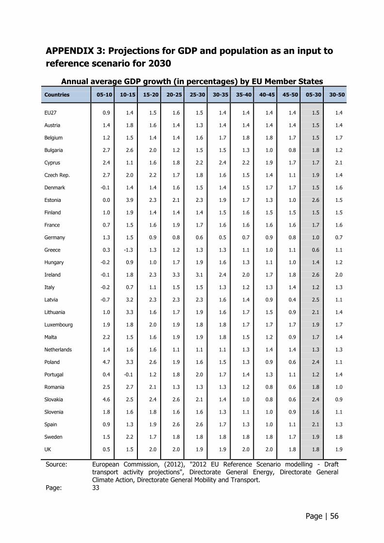
Page | 56

APPENDIX 3: Projections for GDP and population as an input to

reference scenario for 2030

Annual average GDP growth (in percentages) by EU Member States

Countries 05-10 10-15 15-20 20-25 25-30 30-35 35-40 40-45 45-50 05-30 30-50

EU27 Austria Belgium Bulgaria Cyprus Czech Rep. Denmark Estonia Finland France Germany Greece Hungary Ireland Italy Latvia Lithuania Luxembourg Malta Netherlands Poland Portugal Romania Slovakia Slovenia Spain Sweden UK Croatia

0.9

1.4

1.2

2.7

2.4

2.7

-0.1

0.0

1.0

0.7

1.3

0.3

-0.2

-0.1

-0.2

-0.7

1.0

1.9

2.2

1.4

4.7

0.4

2.5

4.6

1.8

0.9

1.5

0.5

0.9

1.4

1.8

1.5

2.6

1.1

2.0

1.4

3.9

1.9

1.5

1.5

-1.3

0.9

1.8

0.7

3.2

3.3

1.8

1.5

1.6

3.3

-0.1

2.7

2.5

1.6

1.3

2.2

1.5

2.1

1.5

1.6

1.4

2.0

1.6

2.2

1.4

2.3

1.4

1.6

0.9

1.3

1.0

2.3

1.1

2.3

1.6

2.0

1.6

1.6

2.6

1.2

2.1

2.4

1.8

1.9

1.7

2.0

2.1

1.6

1.4

1.4

1.2

1.8

1.7

1.6

2.1

1.4

1.9

0.8

1.2

1.7

3.3

1.5

2.3

1.7

1.9

1.9

1.1

1.9

1.8

1.3

2.6

1.6

2.6

1.8

2.0

1.9

1.5

1.3

1.6

1.5

2.2

1.8

1.5

2.3

1.4

1.7

0.6

1.3

1.9

3.1

1.5

2.3

1.9

1.8

1.9

1.1

1.6

2.0

1.3

2.1

1.6

2.6

1.8

1.9

1.7

1.4

1.4

1.7

1.5

2.4

1.6

1.4

1.9

1.5

1.6

0.5

1.3

1.6

2.4

1.3

1.6

1.6

1.8

1.8

1.1

1.5

1.7

1.3

1.4

1.3

1.7

1.8

1.9

1.7

1.4

1.4

1.8

1.3

2.2

1.5

1.5

1.7

1.6

1.6

0.7

1.1

1.3

2.0

1.2

1.4

1.7

1.7

1.5

1.3

1.3

1.4

1.2

1.0

1.1

1.3

1.8

2.0

1.1

1.4

1.4

1.8

1.0

1.9

1.4

1.7

1.3

1.5

1.6

0.9

1.0

1.1

1.7

1.3

0.9

1.5

1.7

1.2

1.4

0.9

1.3

0.8

0.8

1.0

1.0

1.8

2.0

1.0

1.4

1.4

1.7

0.8

1.7

1.1

1.7

1.0

1.5

1.6

0.8

1.1

1.0

1.8

1.4

0.4

0.9

1.7

0.9

1.4

0.6

1.1

0.6

0.6

0.9

1.1

1.7

1.8

0.9

1.5

1.5

1.5

1.8

1.7

1.9

1.5

2.6

1.5

1.7

1.0

0.6

1.4

2.6

1.2

2.5

2.1

1.9

1.7

1.3

2.4

1.2

1.8

2.4

1.6

2.1

1.9

1.8

2.0

1.4

1.4

1.7

1.2

2.1

1.4

1.6

1.5

1.5

1.6

0.7

1.1

1.2

2.0

1.3

1.1

1.4

1.7

1.4

1.3

1.1

1.4

1.0

0.9

1.1

1.3

1.8

1.9

1.2 Source: European Commission, (2012), "2012 EU Reference Scenario modelling - Draft



Page: 33

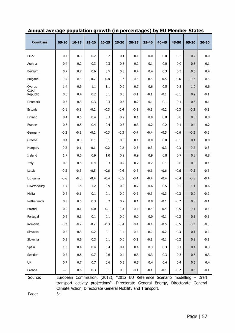
Page | 57

Annual average population growth (in percentages) by EU Member States

Countries

05-10

10-15

15-20

20-25

25-30

30-35

35-40

40-45

45-50

05-30

30-50

EU27 Austria Belgium Bulgaria Cyprus Czech Republic Denmark Estonia Finland France Germany Greece Hungary Ireland Italy Latvia Lithuania Luxembourg Malta Netherlands Poland Portugal Romania Slovakia Slovenia Spain Sweden UK Croatia

0.4

0.4

0.7

-0.5

1.4

0.6

0.5

-0.1

0.4

0.6

-0.2

0.4

-0.2

1.7

0.6

-0.5

-0.6

1.7

0.6

0.3

0.0

0.2

-0.2

0.2

0.5

1.3

0.7

0.7 ---

0.3

0.2

0.7

-0.5

0.9

0.4

0.3

-0.1

0.5

0.5

-0.2

0.3

-0.1

0.6

0.5

-0.5

-0.5

1.5

-0.1

0.5

0.1

0.1

-0.2

0.3

0.6

0.4

0.8

0.7

0.6

0.2

0.3

0.6

-0.7

1.1

0.2

0.3

-0.2

0.4

0.4

-0.2

0.1

-0.1

0.9

0.4

-0.5

-0.4

1.2

0.1

0.3

0.0

0.1

-0.2

0.2

0.3

0.4

0.7

0.7

0.3

0.2

0.3

0.5

-0.8

1.1

0.1

0.3

-0.3

0.3

0.4

-0.3

0.1

-0.2

1.0

0.3

-0.6

-0.4

0.9

0.1

0.2

-0.1

0.1

-0.3

0.1

0.1

0.4

0.6

0.6

0.1

0.1

0.3

0.5

-0.7

0.9

0.0

0.3

-0.4

0.2

0.3

-0.3

0.0

-0.2

0.9

0.2

-0.6

-0.5

0.8

0.0

0.2

-0.3

0.0

-0.4

-0.1

0.0

0.4

0.4

0.5

0.0

0.1

0.2

0.4

-0.6

0.7

-0.1

0.2

-0.3

0.1

0.3

-0.4

0.1

-0.3

0.9

0.2

-0.6

-0.4

0.7

-0.2

0.1

-0.4

0.0

-0.4

-0.2

-0.1

0.4

0.3

0.5

-0.1

0.0

0.1

0.4

-0.5

0.6

-0.1

0.1

-0.3

0.0

0.2

-0.4

0.0

-0.3

0.9

0.2

-0.6

-0.4

0.6

-0.3

0.0

-0.4

0.0

-0.4

-0.2

-0.1

0.3

0.3

0.4

-0.1

0.0

0.0

0.3

-0.5

0.5

-0.1

0.1

-0.2

0.0

0.2

-0.5

0.0

-0.3

0.8

0.1

-0.6

-0.4

0.5

-0.3

-0.1

-0.4

-0.1

-0.5

-0.2

-0.1

0.3

0.3

0.4

-0.1

-0.1

0.0

0.3

-0.6

0.5

-0.1

0.1

-0.3

0.0

0.1

-0.6

-0.1

-0.3

0.7

0.0

-0.6

-0.4

0.5

-0.3

-0.2

-0.5

-0.2

-0.5

-0.3

-0.2

0.1

0.3

0.4

-0.2

0.2

0.3

0.6

-0.7

1.0

0.2

0.3

-0.2

0.3

0.4

-0.3

0.1

-0.2

0.8

0.3

-0.5

-0.5

1.1

0.0

0.3

-0.1

0.1

-0.3

0.1

0.3

0.4

0.6

0.6

0.3

0.0

0.1

0.4

-0.6

0.6

-0.1

0.1

-0.3

0.0

0.2

-0.5

0.0

-0.3

0.8

0.1

-0.6

-0.4

0.6

-0.2

-0.1

-0.4

-0.1

-0.5

-0.2

-0.1

0.3

0.3

0.4

-0.1

Source: European Commission, (2012), "2012 EU Reference Scenario modelling - Draft



Page: 34

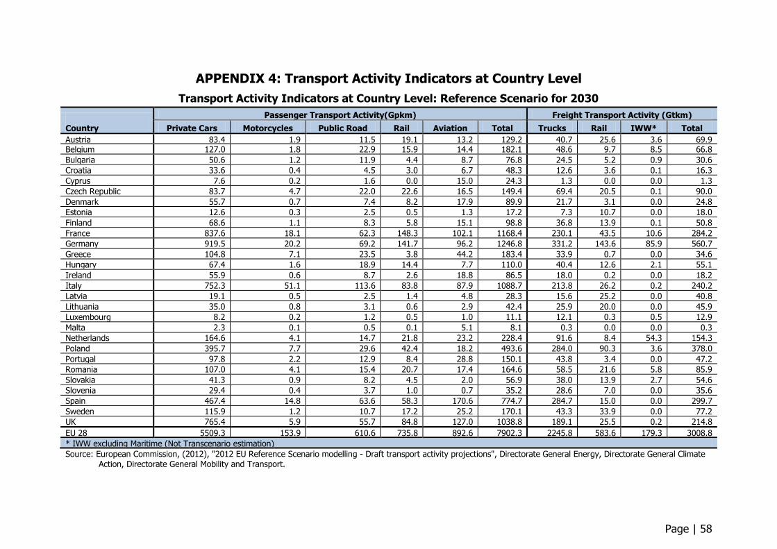
Page | 58

APPENDIX 4: Transport Activity Indicators at Country Level

Transport Activity Indicators at Country Level: Reference Scenario for 2030

Country

Passenger Transport Activity(Gpkm) Freight Transport Activity (Gtkm)

Private Cars Motorcycles Public Road Rail Aviation Total Trucks Rail IWW* Total

Austria 83.4 1.9 11.5 19.1 13.2 129.2 40.7 25.6 3.6 69.9 Belgium 127.0 1.8 22.9 15.9 14.4 182.1 48.6 9.7 8.5 66.8

Bulgaria 50.6 1.2 11.9 4.4 8.7 76.8 24.5 5.2 0.9 30.6

Croatia 33.6 0.4 4.5 3.0 6.7 48.3 12.6 3.6 0.1 16.3

Cyprus 7.6 0.2 1.6 0.0 15.0 24.3 1.3 0.0 0.0 1.3

Czech Republic 83.7 4.7 22.0 22.6 16.5 149.4 69.4 20.5 0.1 90.0

Denmark 55.7 0.7 7.4 8.2 17.9 89.9 21.7 3.1 0.0 24.8

Estonia 12.6 0.3 2.5 0.5 1.3 17.2 7.3 10.7 0.0 18.0

Finland 68.6 1.1 8.3 5.8 15.1 98.8 36.8 13.9 0.1 50.8

France 837.6 18.1 62.3 148.3 102.1 1168.4 230.1 43.5 10.6 284.2

Germany 919.5 20.2 69.2 141.7 96.2 1246.8 331.2 143.6 85.9 560.7

Greece 104.8 7.1 23.5 3.8 44.2 183.4 33.9 0.7 0.0 34.6

Hungary 67.4 1.6 18.9 14.4 7.7 110.0 40.4 12.6 2.1 55.1

Ireland 55.9 0.6 8.7 2.6 18.8 86.5 18.0 0.2 0.0 18.2

Italy 752.3 51.1 113.6 83.8 87.9 1088.7 213.8 26.2 0.2 240.2

Latvia 19.1 0.5 2.5 1.4 4.8 28.3 15.6 25.2 0.0 40.8

Lithuania 35.0 0.8 3.1 0.6 2.9 42.4 25.9 20.0 0.0 45.9

Luxembourg 8.2 0.2 1.2 0.5 1.0 11.1 12.1 0.3 0.5 12.9

Malta 2.3 0.1 0.5 0.1 5.1 8.1 0.3 0.0 0.0 0.3

Netherlands 164.6 4.1 14.7 21.8 23.2 228.4 91.6 8.4 54.3 154.3

Poland 395.7 7.7 29.6 42.4 18.2 493.6 284.0 90.3 3.6 378.0

Portugal 97.8 2.2 12.9 8.4 28.8 150.1 43.8 3.4 0.0 47.2

Romania 107.0 4.1 15.4 20.7 17.4 164.6 58.5 21.6 5.8 85.9

Slovakia 41.3 0.9 8.2 4.5 2.0 56.9 38.0 13.9 2.7 54.6

Slovenia 29.4 0.4 3.7 1.0 0.7 35.2 28.6 7.0 0.0 35.6

Spain 467.4 14.8 63.6 58.3 170.6 774.7 284.7 15.0 0.0 299.7

Sweden 115.9 1.2 10.7 17.2 25.2 170.1 43.3 33.9 0.0 77.2

UK 765.4 5.9 55.7 84.8 127.0 1038.8 189.1 25.5 0.2 214.8

EU 28 5509.3 153.9 610.6 735.8 892.6 7902.3 2245.8 583.6 179.3 3008.8

* IWW excluding Maritime (Not Transcenario estimation)

Source: European Commission, (2012), "2012 EU Reference Scenario modelling - Draft transport activity projections", Directorate General Energy, Directorate General Climate Action, Directorate General Mobility and Transport.

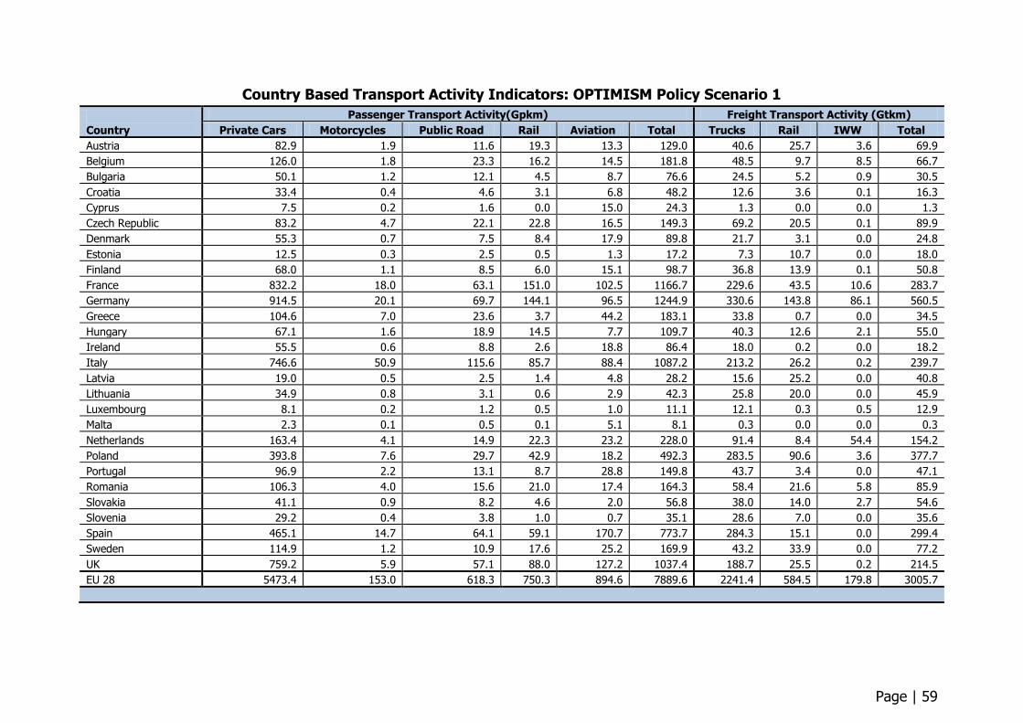
Page | 59

Country Based Transport Activity Indicators: OPTIMISM Policy Scenario 1

Country


Private Cars Motorcycles Public Road Rail Aviation Total Trucks Rail IWW Total

Austria 82.9 1.9 11.6 19.3 13.3 129.0 40.6 25.7 3.6 69.9

Belgium 126.0 1.8 23.3 16.2 14.5 181.8 48.5 9.7 8.5 66.7

Bulgaria 50.1 1.2 12.1 4.5 8.7 76.6 24.5 5.2 0.9 30.5

Croatia 33.4 0.4 4.6 3.1 6.8 48.2 12.6 3.6 0.1 16.3

Cyprus 7.5 0.2 1.6 0.0 15.0 24.3 1.3 0.0 0.0 1.3

Czech Republic 83.2 4.7 22.1 22.8 16.5 149.3 69.2 20.5 0.1 89.9

Denmark 55.3 0.7 7.5 8.4 17.9 89.8 21.7 3.1 0.0 24.8

Estonia 12.5 0.3 2.5 0.5 1.3 17.2 7.3 10.7 0.0 18.0

Finland 68.0 1.1 8.5 6.0 15.1 98.7 36.8 13.9 0.1 50.8

France 832.2 18.0 63.1 151.0 102.5 1166.7 229.6 43.5 10.6 283.7

Germany 914.5 20.1 69.7 144.1 96.5 1244.9 330.6 143.8 86.1 560.5

Greece 104.6 7.0 23.6 3.7 44.2 183.1 33.8 0.7 0.0 34.5

Hungary 67.1 1.6 18.9 14.5 7.7 109.7 40.3 12.6 2.1 55.0

Ireland 55.5 0.6 8.8 2.6 18.8 86.4 18.0 0.2 0.0 18.2

Italy 746.6 50.9 115.6 85.7 88.4 1087.2 213.2 26.2 0.2 239.7

Latvia 19.0 0.5 2.5 1.4 4.8 28.2 15.6 25.2 0.0 40.8

Lithuania 34.9 0.8 3.1 0.6 2.9 42.3 25.8 20.0 0.0 45.9

Luxembourg 8.1 0.2 1.2 0.5 1.0 11.1 12.1 0.3 0.5 12.9

Malta 2.3 0.1 0.5 0.1 5.1 8.1 0.3 0.0 0.0 0.3

Netherlands 163.4 4.1 14.9 22.3 23.2 228.0 91.4 8.4 54.4 154.2

Poland 393.8 7.6 29.7 42.9 18.2 492.3 283.5 90.6 3.6 377.7

Portugal 96.9 2.2 13.1 8.7 28.8 149.8 43.7 3.4 0.0 47.1

Romania 106.3 4.0 15.6 21.0 17.4 164.3 58.4 21.6 5.8 85.9

Slovakia 41.1 0.9 8.2 4.6 2.0 56.8 38.0 14.0 2.7 54.6

Slovenia 29.2 0.4 3.8 1.0 0.7 35.1 28.6 7.0 0.0 35.6

Spain 465.1 14.7 64.1 59.1 170.7 773.7 284.3 15.1 0.0 299.4

Sweden 114.9 1.2 10.9 17.6 25.2 169.9 43.2 33.9 0.0 77.2

UK 759.2 5.9 57.1 88.0 127.2 1037.4 188.7 25.5 0.2 214.5

EU 28 5473.4 153.0 618.3 750.3 894.6 7889.6 2241.4 584.5 179.8 3005.7

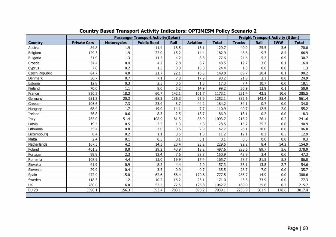
Page | 60


Country



Austria 84.8 1.9 11.4 18.5 13.1 129.7 40.9 25.5 3.6 70.0

Belgium 129.5 1.9 22.0 15.2 14.4 182.9 48.8 9.7 8.4 66.9

Bulgaria 51.9 1.3 11.5 4.2 8.8 77.6 24.6 5.2 0.9 30.7

Croatia 34.4 0.4 4.2 2.8 6.7 48.5 12.7 3.6 0.1 16.4

Cyprus 7.8 0.2 1.5 0.0 15.0 24.4 1.3 0.0 0.0 1.3

Czech Republic 84.7 4.8 21.7 22.1 16.5 149.8 69.7 20.4 0.1 90.2

Denmark 56.7 0.7 7.1 7.8 17.9 90.2 21.8 3.1 0.0 24.9

Estonia 12.8 0.3 2.5 0.5 1.3 17.3 7.4 10.7 0.0 18.1

Finland 70.0 1.1 8.0 5.2 14.9 99.2 36.9 13.9 0.1 50.9

France 850.3 18.3 60.7 142.1 101.7 1173.1 231.4 43.5 10.6 285.5

Germany 931.3 20.3 68.3 136.3 95.9 1252.1 332.6 143.4 85.4 561.4

Greece 105.6 7.3 23.4 3.7 44.2 184.2 34.1 0.7 0.0 34.8

Hungary 68.4 1.7 19.0 14.1 7.7 110.9 40.7 12.5 2.0 55.2

Ireland 56.8 0.6 8.3 2.5 18.7 86.9 18.1 0.2 0.0 18.3

Italy 765.0 51.4 108.9 81.5 86.9 1093.7 215.2 26.1 0.2 241.6

Latvia 19.4 0.5 2.5 1.3 4.8 28.5 15.7 25.2 0.0 40.9

Lithuania 35.4 0.8 3.0 0.6 2.9 42.7 26.1 20.0 0.0 46.0

Luxembourg 8.4 0.2 1.1 0.5 1.0 11.2 12.1 0.3 0.5 12.9

Malta 2.4 0.1 0.5 0.1 5.1 8.1 0.3 0.0 0.0 0.3

Netherlands 167.5 4.2 14.3 20.4 23.2 229.5 92.2 8.4 54.2 154.9

Poland 401.3 8.0 29.2 40.9 18.2 497.6 285.6 89.7 3.6 378.9

Portugal 99.9 2.3 12.4 7.6 28.8 150.9 43.9 3.4 0.0 47.3

Romania 108.9 4.4 15.0 19.9 17.4 165.7 58.7 21.5 5.8 86.0

Slovakia 41.9 0.9 8.2 4.4 2.0 57.3 38.1 13.8 2.7 54.6

Slovenia 29.9 0.4 3.5 0.9 0.7 35.5 28.7 7.0 0.0 35.7

Spain 472.9 15.0 62.6 56.4 170.6 777.5 285.7 14.9 0.0 300.6

Sweden 118.3 1.2 10.2 16.2 25.1 171.0 43.5 33.9 0.0 77.3

UK 780.0 6.0 52.5 77.5 126.8 1042.7 189.9 25.6 0.2 215.7

EU 28 5596.1 156.3 593.4 703.1 890.2 7939.1 2256.9 581.9 178.6 3017.4

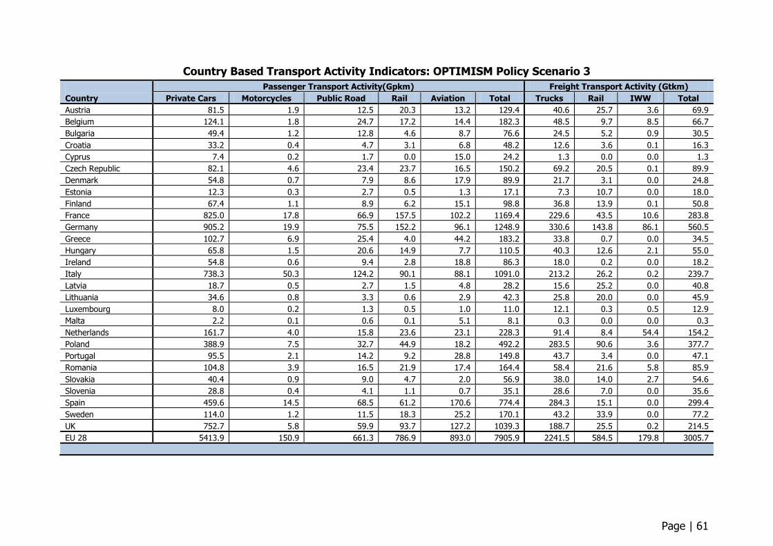
Page | 61


Country



Austria 81.5 1.9 12.5 20.3 13.2 129.4 40.6 25.7 3.6 69.9

Belgium 124.1 1.8 24.7 17.2 14.4 182.3 48.5 9.7 8.5 66.7

Bulgaria 49.4 1.2 12.8 4.6 8.7 76.6 24.5 5.2 0.9 30.5

Croatia 33.2 0.4 4.7 3.1 6.8 48.2 12.6 3.6 0.1 16.3

Cyprus 7.4 0.2 1.7 0.0 15.0 24.2 1.3 0.0 0.0 1.3

Czech Republic 82.1 4.6 23.4 23.7 16.5 150.2 69.2 20.5 0.1 89.9

Denmark 54.8 0.7 7.9 8.6 17.9 89.9 21.7 3.1 0.0 24.8

Estonia 12.3 0.3 2.7 0.5 1.3 17.1 7.3 10.7 0.0 18.0

Finland 67.4 1.1 8.9 6.2 15.1 98.8 36.8 13.9 0.1 50.8

France 825.0 17.8 66.9 157.5 102.2 1169.4 229.6 43.5 10.6 283.8

Germany 905.2 19.9 75.5 152.2 96.1 1248.9 330.6 143.8 86.1 560.5

Greece 102.7 6.9 25.4 4.0 44.2 183.2 33.8 0.7 0.0 34.5

Hungary 65.8 1.5 20.6 14.9 7.7 110.5 40.3 12.6 2.1 55.0

Ireland 54.8 0.6 9.4 2.8 18.8 86.3 18.0 0.2 0.0 18.2

Italy 738.3 50.3 124.2 90.1 88.1 1091.0 213.2 26.2 0.2 239.7

Latvia 18.7 0.5 2.7 1.5 4.8 28.2 15.6 25.2 0.0 40.8

Lithuania 34.6 0.8 3.3 0.6 2.9 42.3 25.8 20.0 0.0 45.9

Luxembourg 8.0 0.2 1.3 0.5 1.0 11.0 12.1 0.3 0.5 12.9

Malta 2.2 0.1 0.6 0.1 5.1 8.1 0.3 0.0 0.0 0.3

Netherlands 161.7 4.0 15.8 23.6 23.1 228.3 91.4 8.4 54.4 154.2

Poland 388.9 7.5 32.7 44.9 18.2 492.2 283.5 90.6 3.6 377.7

Portugal 95.5 2.1 14.2 9.2 28.8 149.8 43.7 3.4 0.0 47.1

Romania 104.8 3.9 16.5 21.9 17.4 164.4 58.4 21.6 5.8 85.9

Slovakia 40.4 0.9 9.0 4.7 2.0 56.9 38.0 14.0 2.7 54.6

Slovenia 28.8 0.4 4.1 1.1 0.7 35.1 28.6 7.0 0.0 35.6

Spain 459.6 14.5 68.5 61.2 170.6 774.4 284.3 15.1 0.0 299.4

Sweden 114.0 1.2 11.5 18.3 25.2 170.1 43.2 33.9 0.0 77.2

UK 752.7 5.8 59.9 93.7 127.2 1039.3 188.7 25.5 0.2 214.5

EU 28 5413.9 150.9 661.3 786.9 893.0 7905.9 2241.5 584.5 179.8 3005.7

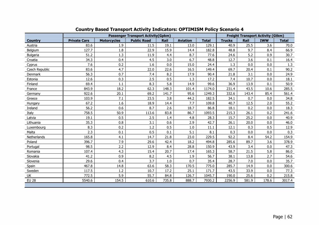
Page | 62


Country



Austria 83.6 1.9 11.5 19.1 13.0 129.1 40.9 25.5 3.6 70.0

Belgium 127.7 1.8 22.9 15.9 14.4 182.8 48.8 9.7 8.4 66.9

Bulgaria 51.2 1.3 11.9 4.4 8.7 77.6 24.6 5.2 0.9 30.7

Croatia 34.3 0.4 4.5 3.0 6.7 48.8 12.7 3.6 0.1 16.4

Cyprus 7.6 0.2 1.6 0.0 15.0 24.4 1.3 0.0 0.0 1.3

Czech Republic 83.6 4.7 22.0 22.6 16.5 149.4 69.7 20.4 0.1 90.2

Denmark 56.3 0.7 7.4 8.2 17.9 90.4 21.8 3.1 0.0 24.9

Estonia 12.6 0.3 2.5 0.5 1.3 17.2 7.4 10.7 0.0 18.1

Finland 69.4 1.1 8.3 5.8 14.9 99.6 36.9 13.9 0.1 50.9

France 843.9 18.2 62.3 148.3 101.4 1174.0 231.4 43.5 10.6 285.5

Germany 922.6 20.1 69.2 141.7 95.6 1249.3 332.6 143.4 85.4 561.4

Greece 103.9 7.1 23.5 3.8 44.2 182.5 34.1 0.7 0.0 34.8

Hungary 67.2 1.6 18.9 14.4 7.7 109.8 40.7 12.5 2.0 55.2

Ireland 56.2 0.6 8.7 2.6 18.7 86.8 18.1 0.2 0.0 18.3

Italy 758.5 50.9 113.6 83.8 86.7 1093.5 215.3 26.1 0.2 241.6

Latvia 19.1 0.5 2.5 1.4 4.8 28.3 15.7 25.2 0.0 40.9

Lithuania 35.3 0.8 3.1 0.6 2.9 42.7 26.1 20.0 0.0 46.0

Luxembourg 8.3 0.2 1.2 0.5 1.0 11.1 12.1 0.3 0.5 12.9

Malta 2.3 0.1 0.5 0.1 5.1 8.1 0.3 0.0 0.0 0.3

Netherlands 165.8 4.1 14.7 21.8 23.0 229.5 92.2 8.4 54.2 154.9

Poland 396.7 7.9 29.6 42.4 18.2 494.8 285.6 89.7 3.6 378.9

Portugal 98.5 2.2 12.9 8.4 28.8 150.9 43.9 3.4 0.0 47.3

Romania 107.4 4.3 15.4 20.7 17.4 165.3 58.7 21.5 5.8 86.0

Slovakia 41.2 0.9 8.2 4.5 1.9 56.7 38.1 13.8 2.7 54.6

Slovenia 29.6 0.4 3.7 1.0 0.7 35.4 28.7 7.0 0.0 35.7

Spain 467.8 14.8 63.6 58.3 170.5 775.0 285.7 14.9 0.0 300.6

Sweden 117.5 1.2 10.7 17.2 25.1 171.7 43.5 33.9 0.0 77.3

UK 772.5 5.9 55.7 84.8 126.7 1045.7 190.0 25.6 0.2 215.8

EU 28 5540.6 154.5 610.6 735.8 888.7 7930.2 2256.9 581.9 178.6 3017.4

European Commission

EUR 26238 – Joint Research Centre –Institute for Prospective Technological Studies

Title: Modelling Future Mobility - Scenario Simulation at Macro Level

Author(s): Mert Kompil, Panayotis Christidis, Hector G. Lopez-Ruiz, Sven Maerivoet, Joko Purwanto and Marco V. Salucci

Luxembourg: Publications Office of the European Union

2013 – 62 pp. – 21.0 x 29.7 cm

EUR – Scientific and Technical Research series – ISSN 1831-9424 (online)

ISBN 978-92-79-33889-2 (pdf)

doi:10.2791/29292

Abstract

The aim of the report is to simulate policy scenarios for passenger transport using Europe-wide transport models, estimate their potential impacts

and demonstrate how do they differ from each other and from the reference scenario for 2030. In more detail, the main objectives of the

deliverable can be given as follows:

to model future multi-modal mobility scenarios for passengers formulated within the previous tasks of the project,

to simulate impacts of identified trends and selected strategies on demand, supply and technology at macro level,

to analyse impacts of selected policies and identified trends on mobility patterns such as in travel demand and modal split,

to estimate potential impacts of selected policy measures on environmental indicators via transport emissions and vehicle fleet sizes,

to compare impacts of different scenario options in quantitative terms and provide useful insights for exploring best policy scenarios

and strategies for sustainable passenger transport.

The research has been conducted under the OPTIMISM project which was received funding from the European Union's Seventh Framework

Programme (FP7/2007-2013), grant agreement n° 284892. The report has been produced as the OPTIMISM project deliverable 3.4: Modelling

Future Mobility - Scenario Simulation at Macro Level.

z

As the Commission’s in-house science service, the Joint Research Centre’s mission is to provide EU policies with independent, evidence-based scientific and technical support throughout the whole policy cycle. Working in close cooperation with policy Directorates-General, the JRC addresses key societal challenges while stimulating innovation through developing new standards, methods and tools, and sharing and transferring its know-how to the Member States and international community. Key policy areas include: environment and climate change; energy and transport; agriculture and food security; health and consumer protection; information society and digital agenda; safety and security including nuclear; all supported through a cross-cutting and multi-disciplinary approach.

LF-NA-26238-EN

-N

Modelling Future Mobility - Scenario Simulation at Macro...

Documents

Transcript of Modelling Future Mobility - Scenario Simulation at Macro...