Modelling & Forecasting of Re/$ Exchange rate – An ... rate paper april...1 | Page Modelling &...
45
1 | Page Modelling & Forecasting of Re/$ Exchange rate – An empirical analysis Surendra babu Gadwala(IIT K) and Somesh K Mathur(Associate Professor,HSS,IITK) April 2014
Transcript of Modelling & Forecasting of Re/$ Exchange rate – An ... rate paper april...1 | Page Modelling &...

1 | P a g e
Modelling & Forecasting of Re/$ Exchange rate – An empirical
analysis
Surendra babu Gadwala(IIT K) and Somesh K Mathur(Associate Professor,HSS,IITK)
April 2014

2 | P a g e
CONTENTS
1 Introduction .........................................................................................................................3
2 Evolution of exchange rate policy in last 50 years ................................................................4
3 Theoretical Framework ........................................................................................................6
4.1 Purchasing power parity theorem (PPP): .......................................................................6
4.2 Harrod balassa samuelson model [1]: ...........................................................................7
4.3 Open interest differential: .............................................................................................8
4.4 Theory : capital flows, forward premium , order flows, rbi intervention ......................10
5 Literature review ...............................................................................................................11
5.1 Literature on modelling and forecasting of exchange rate...........................................11
5.2 Literature on Methodology (ARDL, ARIMA) .................................................................12
6 Model and hypothesis........................................................................................................13
7 Econometric Methodology .................................................................................................14
8 Results ...............................................................................................................................23
8.1 Results: Modelling of Exchange Rate ...........................................................................23
8.2 Results: Forecasting of Exchange rate .........................................................................29
9 Conclusions ........................................................................................................................33
10 Data sources and its definitions .........................................................................................34
11 References .........................................................................................................................35
12 Appendix ...........................................................................................................................36

3 | P a g e
1 INTRODUCTION
The exchange rate is price of one currency in terms of other. It is a key financial variable
that effects decisions made by foreign exchange investors, exporters, bankers, financial
institutions, policy makers. Exchange rate fluctuations affect the value of international
investment portfolios, competitiveness of exports and imports, value of international reserves,
currency value of debt payments, and the cost to tourists in terms of the value of their currency.
Movements in exchange rates thus have important implications for the economy’s business
cycle, trade and capital flows and are therefore crucial for understanding financial
developments and changes in economic policy. Exchange rate virtually determines the terms of
trade with other countries. Stable Exchange Rate is one of the requirements for stable Economy.
India follows the Liberalized Exchange Rate Management System (LERMS), under which it is
absolutely necessary to understand how the exchange rate moves, and why? The market or the
day-today exchange rates, however, are subject to fluctuations in response to the changes to
the supply and demand for international money transfers. There are a host of factors which
influence to the supply and demand for foreign exchange and thus are responsible for the
fluctuations in the rate of exchange Timely forecasts of exchange rates can therefore provide
valuable information to decision makers and participants in the spheres of international finance,
trade and policy making. Nevertheless, we have enough empirical literature is skeptical about
the possibility of accurately predicting exchange rates
This study attempts to develop a model for the rupee-dollar exchange rate taking into
account the different monetary models and variables. The focus is on the exchange rate of the
Indian rupee vis-à-vis the US dollar, i.e., the Re/$ rate. This study covers topics: modelling and
forecasting the exchange rate. There are a host of factors which influence to the supply and
demand for foreign exchange and thus are responsible for the fluctuations in the rate of
exchange.
With Liberalization and development of foreign exchange and assets markets variables
such as capital inflows, forward premium have also become important in determining exchange
rate. From the paper by Medeiros, 2005; Bjonnes and Rime 2003 it was evident that agents in
4 | P a g e
the foreign exchange market have access to private information about fundamentals or
liquidity which is reflected in the buying and selling transactions they undertake that is termed
as order flows which is also show impact on exchange rate. Another important variable in
determining exchange rate is central bank intervention in the foreign exchange market.
After studying the factors affecting the exchange rate in the first part, then in the
second part attempts to examine the forecasting performance of this developed model using
simple Ordinary least squares, Vector auto regression and Autoregressive Integrated Moving
average models. This Study also evaluates the forecasting performance of OLS, VAR, ARIMA
models using different error statistics. We used monthly data of all variables from January 1999
to December 2012 while out of sample forecasting performance evaluated from January 2013
to December 2013 and compared with actual data of exchange rate. Using the best forecasting
model out of all the three models we forecasted exchange rate for future coming months
January 2014 to June 2014.
Against this backdrop, Section II the economic theory and review of literature
would be covered.In Section III, theoretical background for variables in determining exchange
rate Review of literature related to modelling of exchange rate and literature on methodology
are covered in Section IV. Model for this study is in Section V while the econometric
methodology is discussed in Section VI. The estimation and results is done in Section VII. The
Section VIII presents some concluding observations.
2 EVOLUTION OF EXCHANGE RATE POLICY IN LAST 50 YEARS
India’s exchange rate policy has evolved from last 50 years with the gradual opening up
economy since 1990s. In the post-independenceperiod, India’s exchange rate policy has seen a
shift from a par value system to basket peg and further to a managed float exchange rate
system. From 1947 to 1977, India followed par value system where Rupee’s external par value
fixed at 4.15grains of gold. RBI used to maintain this values using Pound sterling as intervention
currency. The Exchange control measures in this fixed exchange rate regime were guided by the
Foreign Exchange Regulation Act that was initially enacted in 1947 and placed on a permanent

5 | P a g e
basis in 1957[1]. Based on the provisions of the Act, the Reserves Bank of India in certain cases
in the central government, controlled and regulated the dealing in foreign exchange payment
outside India, export and import of currency notes and bullion, transfers of securities between
residents and nonresidents, acquisition of foreign securities, etc.[1]
Figure.2.1 - History of rupee dollar exchange rate- Source: RBI (2010)
With the breakdown of Bretton woods system in 1971 and floatation of major
currencies, to stabilize the exchange rate rupee was linked to pound sterling. Later in order to
overcome the weakness associated with single currency peg and to ensure the stability of the
exchange rate, the rupee was pegged to basket of currencies in 1975. By the late eighties and
early nineties it was recognized that both macroeconomics policy and structural factors had
contributed to balance of payment difficulties. The two-step adjustment of July 1991effectively
brought to a close the period of pegged exchange rate. Following the recommendations of
Rangarajan Committee to move towards the market determined exchange rate, the Liberalized
Exchange Rate Management System (LERMS) was put in place in March 1992 involving dual
exchange rate system in the interim period [1]. The dual exchange rate system was replaced by
unified exchange rate system in March 1993. From 1993 till now we are in a mixture of these
both policy called Managed floating with Market determining Structure to make country stable.
The unification of the exchange rate of the Indian rupee was an important step to current
account convertibility. The experience with the market determined exchange rate system in
India, since 1993 is generally described as satisfactory as orderliness prevailed in the Indian

6 | P a g e
market during most of the period. The chronology of evolution of exchange rate policy in India
over a timeline is given in below Table 2.1
Year Foreign exchange market and Exchange rate
1947-1971 Par Value system of exchange rate. Rupee’s external par value was fixed in
terms of gold with the pound sterling as the intervention currency
1971 Breakdown of the Bretton-Woods system and floatation of major currencies.
Rupee was linked to the pound sterling in December 1971.
1975 To ensure stability of the Rupee, and avoid the weaknesses associated with a single
currency peg, the Rupee was pegged to a basket of currency. Currency selection and
weight assignment was left to the discretion of the RBI and not publicly announced.
1978 RBI allowed the domestic banks to undertake intra-day trading in foreign
exchange.
1990-92 Balance of Payments crisis
July 1991 To stabilize the foreign exchange market, a two-step downward exchange rate
adjustment was done (9% and 11%). This was a decisive end to the pegged
exchange rate regime.
March 1992 To ease the transition to a market determined exchange rate system, the
Liberalized Exchange Rate Management System (LERMS) was put in place,
which used a dual exchange rate system. This was mostly a transitional system
March 1993 The dual rates converged, and the market determined exchange rate regime
was introduced. All foreign exchange receipts could now be converted
atmarket determined exchange rates
Source: Reserve Bank of India Table 2.1
3 THEORETICAL FRAMEWORK
3.1 PURCHASING POWER PARITY THEOREM (PPP):
It states that the exchange rate between one currency and another is in equilibrium when
their domestic purchasing powers at that rate of exchange are equivalent. PPP says currency
with higher inflation rate is expected to depreciate relative to currency with lower inflation

7 | P a g e
rate.Purchasing Power Parity suggests that Real exchange rate should be constant, so if there is
a large difference in price between two countries for the same product after exchange rate
adjustment, an arbitrage opportunity is created, because the product can be obtained from the
country that sells it for the lower price. Hence the exchange rate is adjusted to keep the real
exchange rate constant.
RER =e�∗
p
Where, RER = real exchange rate, e=exchange rate expressed as the number of foreign
currencies per one unit of home currency, p*=price in foreign country (US), p=price in home
country.
Taking Log and differentiating, exchange rate will depend on differential inflation rate
��
� =
��
� -
��∗
� ��
� = inflation in India,
��∗
� = inflation in US
PPP theory provided a point of reference for the long run exchange rate in many of the modern
exchange rate theories. It was observed that there were deviations from the PP in short run,
but in the long run, PPP holds equilibrium. The reasons for the failure of the PPP have been
attributed to the heterogeneity in the baskets of goods considered for construction of prices
indices in various countries, the transportation cost, and the imperfect competition of goods
market which led to sharp deviation in PPP theory.
3.2 HARROD BALASSA SAMUELSON MODEL [1]:
It rationalized the long run deviations from PPP. According to this model, productivity
differentials are important in explaining exchange rates. They relax PPP assumption and allow
real exchange rates depend on relative price of non-tradable which are function of productivity
differentials. The Purchasing power parity (PPP) condition and the money demand functions of
domestic and foreign countries are assumed to take the forms as below

8 | P a g e
�
�= �(�, �)
�∗
�∗= �(�∗, �∗)
� = �
�∗
where M represents domestic money balances; P is domestic price level; Y is domestic real
income; i denotes domestic interest rate; E is the exchange rate of domestic currency per
unit of foreign currency; and the corresponding variables for foreign country are denoted by
asterisks.
Therefore, we have the monetary approach of exchange rate determination as follows
� = �
�(�, �)
�(�∗, �∗)
�∗
i.e. exchange rate is depending on money supply and output of both domestic and foreign
country.
3.3 OPEN INTEREST DIFFERENTIAL:
A theory in which the interest rate differential between two countries is equal to the
differential between the forward exchange rate and the spot exchange rate. Given the
assumptions of capital mobility and perfect substitutability. Interest Rate Parity suggests that
for there to be no arbitrage opportunities, two assets in two different countries should have
similar interest rates, as long as the risk for each is the same. The basis for this parity is also the
law of one price, in that the purchase of one investment asset in one country should yield the
same returns as the exact same asset in another country, otherwise exchange rates would have
to adjust to make up for the difference.
�
�=
(1 + I�)
(1 + I�)

9 | P a g e
Where, F = forward exchange, S = spot exchange rate, Ih = interest rate in home country
If = interest rate in foreign country (US)
If you invest a unit of domestic currency in the domestic bond, you can expect to come out with
1+r unit of that currency after a year. If you invest a unit of domestic currency in a foreign bond ,
you will obtain 1/π foreign currency units of that bond and can therefore expect to come out
with (1+r*) 1/π units of foreign currency after a year. This is where exchange rate expextations
will come in to equation. To compare the two returns you must forecast the exchange rate that
is likely to prevail a year from now. Denote that expected exchange rate by π* and use it convert
the foreign currency return on the foreign bond. It is (1/π) (1+r*) πe units of domestic currency.
Then use u to define the difference between the two returns
�
П(1+r*)П� – (1+r) = u;
πe = expected nominal exchange rate after 1 year
r* = interest in foreign country,
r = interest rate in home country,
(1/π) (1+r*) πe= revenue that home country gets after 1 year of investment in foreign country, u
= open interest rate differential
П� = П��П
П = expected rate of change of exchange rate
⇒�
П(1+r*)(П�П + П ) – (1+r) = u
⇒ (1+r*)(1+П�) – (1+r) = u
⇒ П�+r*-r = u Higher interest rates attract foreign capital and cause the domestic currency to appreciate and
lower interest rates tend to depreciation. That how the relation between interest rate and
exchange rate was given.

10 | P a g e
3.4 THEORY : CAPITAL FLOWS, FORWARD PREMIUM , ORDER FLOWS, RBI INTERVENTION
With the evolution of exchange rate policy brings more variables that affect exchange
rate because of increase in liberalization and opening up of capital accounts the world over,
capital flows become important variable to consider in analysis. The relations between capital
flows and exchange rate is hypothesized to be negative because capital inflows as purchase of
domestic assets by foreigners and capital outflows means as purchase of foreign assets by
residents. Exchange rate is determined by supply and demand for foreign and domestic assets,
purchase of foreign assets drives of foreign currency. So, an increase of capital inflows lead to
appreciation of the domestic currency when there is no government intervention in the foreign
market exchange.
The forward premium measured by the difference between forward and spot exchange
rate. According to the covered interest parity, the interest rate differential between two
countries equals the premium on forward contracts. So if domestic interest rates rise foreign
currency appreciate. The relation between exchange rate and forward premium is expected to
be positive.
Order flow is the cumulative flow of transactions, signed positively or negatively
depending on whether the initiator of the transaction is buying or selling. Order flow takes
positive values if the agent purchases foreign currency and takes negative values if it sells at the
dealer's bid. Conventionally, order flow is taken as purchase minus sales of foreign currency.
Hence an increase in order flow will generate forces in the foreign exchange market such that
there is pressure on the domestic exchange rate to depreciate. Hence the order flow and the
exchange rate are positively related (Evans and Lyons, 2005).
Intervention by the central bank in the foreign exchange market is also important variable
that show effect on exchange rate. The motive of central bank intervene is to maintain export
competiveness; to reduce volatility and to protect the currency from speculative attacks.
Intervention also influences exchange rate through different channels through portfolio balance,
through monetary channel, intervention accompanies by open market operations, so different

11 | P a g e
channel intervention gives different signs on exchange rate so the overall effect of intervention
on exchange rate is ambiguous.
4 LITERATURE REVIEW
4.1 LITERATURE ON MODELLING AND FORECASTING OF EXCHANGE RATE
Early studies which modelled exchange rates using flexible price model such as
Bilson(1978), Woodbury(1980) and Dornbusch (1984) support the performance of the flexible
price monetary model in modelling of exchange rate. Studies by Driskill and sheffrin (1981)
failed to support the flexible price monetary model and real interest differential model in
modelling exchange rate.
Rakesh mohan(2001)in which he explains various aspects of the capital flows and it policy
implications and explained the capital flow as determinant of exchange rate modelling .Dua and
Sen (2009) develop a model which examines the relationship between the real exchange rate,
level of capital flows, volatility of the flows, fiscal and monetary policy indicators and the
current account surplus, and find that an increase in capital inflows and their volatility lead to
an appreciation of the exchange rate. The theoretical sign on volatility can, however, be
positive or negative.
Kenen(1994), in his book he discusses in how exchange rate of a country is determined by
a host of factors which includes GDP, Inflation, Interest rate, Money supply along with these
there are other’s countries exchange rate which also affects Indian Rupee Exchange Rate.
Numerous factors determine exchange rates, and all are related to the trading relationship
between two countries. Kenen gave a theoretical garphs and relations between variables
differential inflation, interest rate, output, money supply and variables like pound sterling,
euro , yen etc.

12 | P a g e
Pami Dua and Rajiv Ranjan (2012), recent work where they covered the topics various
facets of economic policy with respect to the exchange rate, second the recent global financial
crisis and the role of exchange rate in that; third the pattern of capital flows and capital
account liberalization; fourth modelling and forecasting exchange rate in which they discussed
the exchange rate policy of India in background of capital flows, order flows, central bank
intervention. At latter part they attempted to gauge the ability of economics to forecast using
VAR and BVAR framework and then evaluated the forecast performance.
4.2 LITERATURE ON METHODOLOGY (ARDL, ARIMA)
In recent years, although the long run model of exchange rate determination has
been the subject of interest for many researchers, there have been only limited studies
conducted for the case of Asian countries. To our knowledge, those studies are Makrydakis
(1998) and Miyakoshi (2000) for Korea, Chin et al. (2007) for the Philippines, Husted and
MacDonald (1999) and Chinn (2000a, b) for selected Asian countries. However, these studies
adopted the conventional likelihood-based approach to cointegration proposed by Johansen
and Julius (1990).This approach requires the same order of integration of all variables in the
system, which is hardly satisfied. The purpose of this paper is to fill the gap in the literature by
contributing another study for the case of the Philippines using a state-of-the-art
econometric technique, namely Autoregressive Distributed Lag (ARDL) to cointegration. In
particularly we followed a paper by M.Pesaran, Shin, J.Smith “Bounds testing approaches to the
analysis of level relationships”- in which they proposed tests are based on standard F- and t-
statistics used to test the significance of the lagged levels of the variables in a univariate
equilibrium correction irrespective of variables in I (0) orI (1) through which one can test for
whether there is long run relationship between variables exists or not.
Long and Samreth (2008) , examined the validity of both short and long run monetary
model of exchange rate using method Auto regressive distributed lag model to cointegration.
Pankaj Sinha,Randev, Sushant gupta (2010) analyzed the state of Indian economy pre , during
and post-recession by taking factors such as GDP, Exchange rate, inflation , capital markets and

13 | P a g e
fiscal deficit. They also forecasted some of the major economic variables using ARIMA model.
They found that GDP, foreign investments, fiscal deficit and capital markets to rise in 2010-11
period where as ruppe –dollar exchange rate will not change much during this period of study.
In sum, several exchange rate models available in the literature have been tested the
last two and half decades. Literatures suggest that different papers considered different
monetary models in modelling the exchanges rate however considering more variables giving
better results than the random walk. Keeping all results and variables that past studies taken
into account, this study tries to re model the exchange rate and forecasted for period January
2014- June 2014.
5 MODEL AND HYPOTHESIS
For estimating the degree of dependence of Indian exchange rates (against USD) on market
factors, we have developed a regression model with USD-India exchange rate on left hand side
and a number of economic/market variables on the right hand side.
Our model is as follows
��� = �� + �������� + ������� + ������ + ������� + ��������
+ ��MSIND� + ��GDPIND� + ��CF� + ���OF� + ������
+ ������� + ��������
Where,
EX = Price of US dollar in terms of Indian Rupee
Pound = Exchange rate between Pound and USD
Euro = Exchange rate between Euro and USD
Yen = Exchange rate between Yen and USD
DINF = Differential in inflation rate
DREIR= Differential in interest rate
MSIND = Money Supply in India
GDPIND = GDP in India
CF= Capital Inflows

14 | P a g e
OF= Order Flows
FP= Forward premium
TRB= Trade balance
RBII= Central bank Intervention
Definition of each variable and their data sources were given in appendix. Based on
theory that we have seen in theoretical framework section and also by previous paper results
one can hypothesis the relation between explanatory variables and dependent variable.
The expected signs of variables can be summarized as follows:
Expected signs of independent variables: Dependent variable is EX
Variables Expected Sign
Money supply (MSIND) +
Output ( GDPIND) -
Capital Inflows ( CF ) -
Forward Premium (FP) +
Order Flows (OF) +
Trade Balance (TRB) -/+
Intervention (RBII) -/+
Table 5.1: Expected hypothesis of variables
6 ECONOMETRIC METHODOLOGY
1. Method of least square -Least squares means that the overall solution minimizes the
sum of the squares of the residuals made in solving every single equation.
Since we are dealing here with non-stationary data results produces unreliable t-
statistics of the estimated coefficients and Durbin Watson Test statistic goes to zero which is
evidence of presence of Postive autocorrelations. So we have to overcome these two problems
to get efficient estimates.

15 | P a g e
2. Cochrane-Orcutt – Feasible Generalized Least Squares :
Four Steps to carry out this FGLS method as remedy for serial positive auto correlation
Run OLS on original equation
Regress residuals on lagged residuals to estimate rho.
Transform variables using this estimate of rho.
Run OLS on the transformed variables
1. Begin with a model of a dependent variable Y as a function of s set of independent variables
X1…….Xk
Yt = b0 + b1 X1t + b2 X2t + b3X3t + ... + bkXkt + et [1]
2. Regress et on et-1 to estimate rho, the impact of lag 1 errors on contemporary errors.
et = ρ (et-1) + ut [2]
3. The "trick" in creating this pseudo-GLS estimator is to create a new estimating equation,
transforming the original variables in the process of eliminating the (first order) serial
correlation.
a. Multiple equation 1 by r, estimated in equation 2.
ρYt = ρb0 + ρb1 X1t + ρb2 X2t + ρb3X3t + ... + ρbkXkt + ρet[3a]
b. Lag equation 3a one time period,
ρYt-1 = ρb0 + ρb1 X1,t-1 + ρb2 X2, t-1 + ρb3X3, t-1 + ... + ρbkXk, t-1 + ρet-1[3b]
c. Subtract equation 3b from equation 1.
Yt - ρYt-1 = {b0 + b1 X1t + b2 X2t + b3X3t + ... + bkXkt + et} –
{ρb0 + ρb1 X1,t-1 + ρb2 X2, t-1 + ρb3X3, t-1 + ... + ρbkXk, t-1 + ρet-1}[3c]
d. Simplify by combining terms on the right side.
Yt - ρYt-1 = (1-ρ) b0 + b1(X1t -ρX1,t-1) + … + (et- ret-1)[3d]
e. Remember by equation 2, et = ρet-1 + ut
Yt - ρYt-1 = (1-ρ) b0 + b1(X1t - ρX1,t-1) + … + ut [3e]
We no longer have a serially correlated error term.
f. Simplify 3e by redefining each transformed variable to the right side of the equation.
Y* = Yt - ρYt-1

16 | P a g e
Xi* = Xit - ρXi,t-1
k* = 1-ρ
Y* = b0k* + b1X1* + b2X2*+ … + ut[3f]
4. Using equation 3f, regress Y* on k and the Xi . The Prais-Winston Estimator will give the Co-
FGLS estimates in STATA in which it improves the Durbin Watson statistic.
Unit root tests are used to test for stationarity or order of integration of each series of the
variables (second problem that simple OLS estimates havein case of time series variable)
3. Unit Root Test
The first step of testing cointegration is to test all the time series variables for
stationarity. Therefore, we conducted the Augmented Dickey-Fuller unit root test on each of
the variables and verify that each of these series is integrated of order one.
4. Augmented Dickey-Fuller test
The greater the ADF test statistic value than the critical t-statistical value, stronger the
hypothesis that there is a unit some level of confidence. Non-stationary data used in estimation
produces unreliable t-statistics of the estimated coefficients in method of Least Squares. Unit
root tests are used to test for stationarity or order of integration of each series of the variables.
There are three type of ADF methods to check unit root problem.
Without Constant and Trend ∆Y= δ Y(t-1)+ εt
With Constant ∆Y=α+ δ Y(t-1)+ εt
Without Constant and Trend ∆Y=α+δ Y(t-1)+ βT+ εt
Decision rule:
If t* > ADF critical value ⇒ not reject null hypothesis, i.e., unit root exists.
If t* < ADF critical value ⇒ reject null hypothesis, i.e., unit root does not exist.
If every series is in either I(0) or I(1) we would have apply Johansen cointegration test
and we would have get a non redundant estimates but if series are in different order of
integration I mean some series are I(0) , some are I(1) , some are I(2) so we will end up doing
Pesaran’s Autoregressive distributed lag (ARDL) approach for cointegration

17 | P a g e
5. ARDL approach to cointegration
The basic form of an ARDL regression model is:
yt = β0 + β1yt-1 + .....+ βkyt-p + α0xt + α1xt-1 + α2xt-2 + ....... + αqxt-q + εt , (1)
Where εt is a random "disturbance" term, which we'll assume is "well-behaved" in the usual
sense. In particular, it will be serially independent.
Proof :
A conventional ECM for cointegrated data looks like. It would be of the form:
Δyt = β0 + Σ βiΔyt-i + ΣγjΔx1t-j + ΣδkΔx2t-k + φzt-1 + et(2)
Here, z, the "error-correction term", is the OLS residuals series from the long-run "cointegrating
regression"
yt = α0 + α1x1t + α2x2t + vt (3)
The ranges of summation in (2) are from 1 to p, 0 to q1, and 0 to q2 respectively.
Formulate the following model:
Δyt = β0 + Σ βiΔyt-i + ΣγjΔx1t-j + ΣδkΔx2t-k + θ0yt-1 + θ1x1t-1 + θ2 x2t-1 + et(4)
Notice that this is almost like a traditional ECM. The difference is that we've now
replaced the error-correction term, zt-1 with the terms yt-1, x1t-1, and x2t-1. From (3), we can see
that the lagged residuals series would be zt-1 = (a0 - a1x1t-1 - a2x2t-1), where the a's are the OLS
estimates of the α's. So, what we're doing in equation (4) is including the same lagged levels as
we do in a regular ECM, but we're not restricting their coefficients.
This is why we might call equation (4) an "unrestricted ECM", or an "unconstrained ECM".
Pesaran et al. (2001) call this a "conditional ECM".
6. Bounds Testing
Here's equation (4), again:

18 | P a g e
Δyt = β0 + Σ βiΔyt-i + ΣγjΔx1t-j + ΣδkΔx2t-k + θ0yt-1 + θ1x1t-1 + θ2 x2t-1 + et
All that we're going to do is preform an "F-test" of the hypothesis, H0: θ0 = θ1 = θ2 = 0 ; against
the alternative that H0 is not true. As in conventional cointegration testing, we're testing for
the absence of a long-run equilibrium relationship between the variables. This absence
coincides with zero coefficients for yt-1, x1t-1 and x2t-1 in equation (4). A rejection of H0implies
that we have a long-run relationship.
There is a practical difficulty that has to be addressed when we conduct the F-test. The
distribution of the test statistic is totally non-standard even in the asymptotic case where we
have an infinitely large sample size. (This is somewhat akin to the situation with the Wald test
when we test for Granger non-causality in the presence of non-stationary data. In that case, the
problem is resolved by using the Toda-Yamamoto (1995) procedure, to ensure that the Wald
test statistic is asymptotically chi-square.
Exact critical values for the F-test aren't available for an arbitrary mix of I(0) and I(1)
variables. However, Pesaran et al. (2001) supply bounds on the critical values for asymptotic
distribution of the F-statistic. For various situations (e.g., different numbers of variables, (k + 1)),
they give lower and upper bounds on the critical values. In each case, the lower bound is based
on the assumption that all of the variables are I(0), and the upper bound is based on the
assumption that all of the variables are I(1). In fact, the truth may be somewhere in between
these two polar extremes. If the computed F-statistic falls below the lower bound we would
conclude that the variables are I(0), so no cointegration is possible, by definition. If the F-
statistic exceeds the upper bound, we conclude that we have cointegration. Finally, if the F-
statistic falls between the bounds, the test is inconclusive.
As a cross-check, we should also perform a "Bounds t-test" of H0 : θ0 = 0, against H1 :
θ0 < 0. If the t-statistic for yt-1 in equation (4) is less than the "I(1) bound" tabulated by Pesaran
et al. (2001; pp.303-304), this would support the conclusion that there is a long-run relationship
between the variables. If the t-statistic is greater than the "I(0) bound", we'd conclude that the
data are all stationary.

19 | P a g e
Assuming that the bounds test leads to the conclusion of cointegration, we can meaningfully
estimate the long-run equilibrium relationship between the variables:
yt = α0 + α1x1t + α2x2t + vt(5)
as well as the usual ECM:
Δyt = β0 + Σ βiΔyt-i + ΣγjΔx1t-j + ΣδkΔx2t-k + φzt-1 + et (6)
Where zt-1 = (yt-1 -a0 - a1x1t-1 - a2x2t-1), and the a's are the OLS estimates of the α's in (5).
We can "extract" long-run effects from the unrestricted ECM. Looking back at equation (4), and
noting that at a long-run equilibrium, Δyt = 0, Δx1t = Δx2t = 0, we see that the long-run
coefficients for x1 and x2 are -(θ0 / θ1) and -(θ0 / θ2) respectively.
7. Vector auto regression
Vector auto regression (VAR) is an econometric model used to capture the linear
interdependencies among multiple time series. VAR models generalize the univariate auto
regression (AR) models by allowing for more than one evolving variable. All variables in a VAR
are treated symmetrically in a structural sense; each variable has an equation explaining its
evolution based on its own lags and the lags of the other model variables.
A VAR model describes the evolution of a set of k variables (called endogenous variables) over
the same sample period (t = 1, ..., T) as a linear function of only their past values. The variables
are collected in a k × 1 vector yt, which has as the i th element, yi,t, the time t observation of
the i th variable. For example, if the i th variable is GDP, then yi,t is the value of GDP at time t.
A p-th order VAR, denoted VAR(p), is
yt = c + A1 yt-1 + A2 yt-2+ ….. + Ap yt-p + et
where the l-periods back observation yt−l is called the i-th lag of y, c is a k × 1 vector of constants
(intercepts), Aiis a time-invariant k × k matrix and and it can also express in the following form:

20 | P a g e
(1 − � − �� − ��)�� = � + ��
�(�)�� = � + ���� ~� (0, ٠)
In a VAR, we are often interested in obtaining the impulse response functions. Impulse
responses trace out the response of current and future values of each of the variables to a one-
unit increase (or to a one-standard deviation increase, when the scale matters) in the current
value of one of the VAR errors, assuming that this error returns to zero in subsequent periods
and that all other errors are equal to zero. The implied thought experiment of changing one
error while holding the others constant makes most sense when the errors are uncorrelated
across equations, so impulse responses are typically calculated for recursive and structural
VARs.
�� = �������� + �����
We calculate the IRF’s to a unitshock of u once we know ���. We also used VAR model to
forecast out of sample.
8. Auto Regressive Integrated Moving Average Model
An autoregressive integrated moving average (ARIMA) model is a generalization of an
autoregressive moving average (ARMA) model. These models are fitted to time series data
either to better understand the data or to predict future points in the series (forecasting). They
are applied in some cases where data show evidence of non-stationarity, where an initial
differencing step (corresponding to the "integrated" part of the model) can be applied to
remove the non-stationarity.
The model is generally referred to as an ARIMA(p,d,q) model where parameters p, d,
and q are non-negative integers that refer to the order of the autoregressive, integrated, and
moving average parts of the model respectively. ARIMA models form an important part of the
Box-Jenkins approach to time-series modelling.
Given a time series of data Xt where t is an integer index and the Xt are real numbers, then an
ARMA(p' ,q) model is given by:

21 | P a g e
�1 − � ∝� ��
��
���
� �� = �1 + � ����
�
���
� ��
where L is the lag operator, ∝�the are the parameters of the autoregressive part of the model,
the ��are the parameters of the moving average part and the �� are error terms. The error
terms �� are generally assumed to be independent, identically distributed variables sampled
from a normal distribution with zero mean
Assume now that the polynomial �1 − ∑ ∝� ������� �has a unitary root of multiplicity d. Then it
can be rewritten as:
�1 − � ∝� ��
��
���
� = �1 + � ∅���
����
���
� (1 − �)�
An ARIMA(p,d,q) process expresses this polynomial factorisation property with p=p'−d, and is
given by:
�1 + � ∅���
����
���
� (1 − �)��� = �1 + � ����
�
���
� ��
and thus can be thought as a particular case of an ARMA(p+d,q) process having the
autoregressive polynomial with d unit roots. (For this reason, every ARIMA model with d>0 is
not wide sense stationary.)
The above can be generalized as follows.
�1 + � ∅���
����
���
� (1 − �)��� = � + �1 + � ����
�
���
� ��
This defines an ARIMA(p,d,q) process

22 | P a g e
9. Forecast Error Statistics
Thiel's inequality coefficient, also known as Thiel's U, provides a measure of how well a time
series of estimated values compares to a corresponding time series of observed values. The
statistic measures the degree to which one time series ({Xi}, i = 1,2,3, ...n) differs from another
({Yi}, i = 1, 2, 3, ...n). Thiel's U is calculated as:
Thiel's inequality coefficient is useful for comparing different forecast methods: for
example, whether a fancy forecast is in fact any better than a naïve forecast repeating the last
observed value. The closer the value of U is to zero, the better the forecast method. A value of
1 means the forecast is no better than a naïve guess.The U-statistic measures the ratio of the
Root Mean Square Error (RMSE) of the model forecasts to the RMSE of naive, no-change
forecasts
The RMSE is given by the following formula , If At+ndenotes the actual value of a variable
in period (t+n) , and tFt+nthe forecast made in period t for (t+n), then for T observations
���� = [� (���� − ����)�/��
] �.�
A comparison with the naïve model is, therefore, implicit in the U-statistic. A U-statistic
of 1 indicates that the model forecasts match the performance of naïve, no-change forecasts. A
U-statistic >1 shows that the naïveforecasts outperform the model forecasts. If U is <1, the
forecasts from the model outperform the naïve forecasts. The U-statistic is, therefore, a relative
measure of accuracy and is unit-free.
Summary of Steps in Econometric Estimation

23 | P a g e
In this study, First we run simpleOrdinary Least squares and we checked for
autocorrelation and to overcomethe problem of positive auto correlation we adopted
Cochrane-Orcutt – Feasible Generalized Least Squares. Since we are dealing with time series,
we checked for presence of unit root using augmented Dickey-Fuller test. We then moved to
estimation using either Johansen cointegration or Auto regressive distributed lag methods
based on integrated levels of series.
Second, we forecast the exchange rate using three methods OLS, VAR, ARIMA by
considering the variables which comes significant in the first step. We forecasted for three
different out of sample periods and then we evaluated the forecasting methods by comparing
actual data of exchange rate using Error statistics
7 RESULTS
The Models that we discussed in last section were used to estimate exchange rate in this
section. We will discuss the results in two parts, first part modelling and second part forecasting
7.1 RESULTS: MODELLING OF EXCHANGE RATE
We estimated the model given in section 5 using simple ordinary least squares, it was found
that Durbin Watson test (test for presence of autocorrelation) was less than 2 which indicates
that there is presence of positive autocorrelation in simple OLS. In order to overcome
autocorrelation we employed the Feasible Generalized least squares. The results were show in
table below.
Variables OLS Nonlinear OLS CO- FGLS
Pound 0.269311* 0.280878* 0.28037*

24 | P a g e
Euro -0.187405* -0.112224 -0.11725
Yen 0.127715* 0.076823 0.08196
DINF -5.71E-05 9.73E-06 5.64E-06
DREIR 0.002852 0.002295 0.0023059
MSIND 0.728961* 0.673365* 0.67589*
GDPIND -0.818727* -0.758652* -0.7611358*
CF -0.000561* -0.000174 -0.000172
OF -0.002259* -0.001430* -0.00138*
FP -0.018669 -0.36885* -0.36724*
TRB 0.000135 0.000088 0.000074
RBII -0.000214* -0.0000617* -0.0000583*
AR(1) -------- 0.542795* 0.5194*
R- Squared 0.997017 0.997536 0.9895
Durbin- Watson 1.202654 1.775138 1.74182
Table 7.1.1 : Empirical results of OLS , Co FGLS ( * is significant at 5% level of significance )
Simple OLS results are given in first column of Table 7.1.1 where pound, Euro, Money supply
India, GDP India, Capital flows, Order flows, central bank intervention found significant at 5%
level of significance whereas the estimates are redundant in nature as R-squared value is
almost one and Durbin Watson Test is 1.2 (going to 0) which indicates that there is presence of
unit root problem and auto correlation in simple Ordinary least squares
If we see the sign of significant variables that is price of USD in terms of Rupee
appreciates if pound, yen appreciates and depreciates if euro appreciates (negative sign for
Euro variable).Money supply in India is positively related to exchange rate which means, excess
supply of money leads to reduction in savings its equivalent to excess demand for goods and
securities leads to BOP deficit, if there is deficit then there is flexible exchange rate and you will
see the depreciation of Indian rupee and appreciation of USD. GDP of our country – it comes
with a negative sign because higher the GDP, larger is the demand for money ,more is the
savings, lesser is the demand for goods and securities, there will be BOP surplus, leading to
appreciation of Indian rupee or the depreciation of USD – That’s why we see a negative sign for
GDPIND. Differential inflation rate and real interest rate, Money supply and GDP of US found
insignificant in simple OLS.

25 | P a g e
Capital flows found to be negative which is same as theory suggests that is if there is
more purchase of foreign assets by foreigners then there will more demand for our Indian
rupee which means appreciation of our currency and depreciation of USA dollar.
Conventionallyorder flows and exchange rate are positively related but OLS results found that it
is negative relationship. By definition Order flows is taken as purchase minus sales of foreign
currency so with the negative sign it implies that if incase there is sales of foreign currency is
more than the purchase than with increase of order flows there will be appreciation of our
currency. Variables forward premium and trade balance found insignificant in simple OLS but,
forward premium found to be significant if we remove the autocorrelation problem (column 2,
3,).
After removing problem of autocorrelation the Durbin Watson static increased from 1.2
to 1.7. In Nonlinear, COFGLS methods coefficients of explanatory variables were changed but
their relation with exchange rate was still same as ordinary least squares except for forward
premium. Since all these variables were time dependent variables there may be a unit root
problem in seriesCo- FGLS coefficients are redundant as data series have unit root problem so
we don’t consider coefficient value here. So before we estimate the impact of each variable on
exchange rate we need to check for unit problem.
In order to check stationarity test, we employed Augmented Dickey Fuller test to see the
integrated level of all series so based on this test we found the following integrated levels for
each variable ( results were given in Appendix )
Variables Integrated levels EX I(1)
Pound I(2) Euro I(1) Yen I(1)
DINF I(0) DREIR I(0) MSIND I(1) GDPIND I(1)

26 | P a g e
CF I(0) OF I(0) FP I(1)
TRB I(1) RBII I(0)
Table 7.1.2. Results of ADF test for each independent variable
Table 7.1.2 shows the results of Augmented Dickey Fuller Test which conveys that some
variables are stationary whereas some variables have unit root problem. The variables
differential inflation rate, differential interest rate, capital flows, order flows, central bank
intervention found to be stationary and all other variables are no stationary. Except pound
testing for differences of each non stationary variables are integrated of order one.
One can know the linear interdependencies among multiple time series using Vector Auto
Regressive Method in which we consider two things that Variance Decomposition and Impulse
Response functions
Variance Decomposition: If pound changes how much impact will be there on dependent
variable and in how many time periods
Impulse Response Functions: If you give a shock to system How is my variables affected to after
certain time period – Impulse response functions
Table 7.1.3: Results of variance decomposition

27 | P a g e
In Table 7.1.3, after 10 periods pound rupee exchange rate is explaining 25.6% variability
which is highest among all independent variables, differential interest rate explains 16.8 % and
so on. Likewise one can notice which variable will explain the dependent variable more after
certain periods. Similarly we want to know suppose if there is any shock in one of the variable
then how exchange rate react that shock will capture by impulse response graphs. It was found
from following graph is that for any shock, exchange rate will deviate from equilibrium level and
it will fluctuate for many periods
Figure 7.1.1 Impulse Response functions
From the ADF test results, some variables stationary and some are integrated to order
one. If we would have get all the series integrated to order I(1) then we would have applied
Johansson cointegration. Since some are I(0) and some are I(1), so we will end up doing
Pesaran’s Autoregressive distributed lag (ARDL) approach for cointegration. A series of steps
has to do to reach final ARDL results, one of the step is to do Bound’s test to check whether the
variables are have long run relationship or not. The following figure is the result of bound test
where we compare the F-static with the Pesaran, Shin, Smith calculated critical values.
- 0 . 0 6
- 0 . 0 4
- 0 . 0 2
0 . 0 0
0 . 0 2
0 . 0 4
0 . 0 6
2 4 6 8 1 0 1 2 1 4 1 6 1 8 2 0
Response of EX t o EX
- 0 . 0 6
- 0 . 0 4
- 0 . 0 2
0 . 0 0
0 . 0 2
0 . 0 4
0 . 0 6
2 4 6 8 1 0 1 2 1 4 1 6 1 8 2 0
Response of EX t o POUND
- 0 . 0 6
- 0 . 0 4
- 0 . 0 2
0 . 0 0
0 . 0 2
0 . 0 4
0 . 0 6
2 4 6 8 1 0 1 2 1 4 1 6 1 8 2 0
Response of EX t o EURO
- 0 . 0 6
- 0 . 0 4
- 0 . 0 2
0 . 0 0
0 . 0 2
0 . 0 4
0 . 0 6
2 4 6 8 1 0 1 2 1 4 1 6 1 8
Response of EX t o YEN
- 0 . 0 6
- 0 . 0 4
- 0 . 0 2
0 . 0 0
0 . 0 2
0 . 0 4
0 . 0 6
2 4 6 8 1 0 1 2 1 4 1 6 1 8 2 0
Response of EX t o DI NF
- 0 . 0 6
- 0 . 0 4
- 0 . 0 2
0 . 0 0
0 . 0 2
0 . 0 4
0 . 0 6
2 4 6 8 1 0 1 2 1 4 1 6 1 8 2 0
Response of EX t o DREI R
- 0 . 0 6
- 0 . 0 4
- 0 . 0 2
0 . 0 0
0 . 0 2
0 . 0 4
0 . 0 6
2 4 6 8 1 0 1 2 1 4 1 6 1 8 2 0
Response of EX t o MSI ND
- 0 . 0 6
- 0 . 0 4
- 0 . 0 2
0 . 0 0
0 . 0 2
0 . 0 4
0 . 0 6
2 4 6 8 1 0 1 2 1 4 1 6 1 8
Response of EX t o MSUS
- 0 . 0 6
- 0 . 0 4
- 0 . 0 2
0 . 0 0
0 . 0 2
0 . 0 4
0 . 0 6
2 4 6 8 1 0 1 2 1 4 1 6 1 8 2 0
Response of EX t o GDPI ND
- 0 . 0 6
- 0 . 0 4
- 0 . 0 2
0 . 0 0
0 . 0 2
0 . 0 4
0 . 0 6
2 4 6 8 1 0 1 2 1 4 1 6 1 8 2 0
Response of EX t o GDPUS
Response t o One S. D. I nnovat ions ± 2 S. E.

28 | P a g e
Figure 7.1.2. Bounds test results (wald test)
Wald test gives us with F static value 1.19 at 8 degrees of freedom, and Bounds test
gives us the conditions that If F test > Pesaran Critical hgher bound at degrees of freedom then we
reject H0implies that there is a long-run relationship between exchange rate and variables. If F-Value <
Pesaran Critical Lower bound then there is no Lon run relationship .If F value is in between
Lower and Higher pesaran critical values that is Inconclusive
Table 7.1.4: Critical value for Bounds Test given by Pesaran, Shin, Smith (2001)
At 5% level of significance, for k=8 degree of freedom Pesaran(2001) critical value Lower bound
is 2.55 and higher bound is 3.68 (from Table 7.1.4). From Wald test, F static is 1.19 which is less
than lower critical bound (2.55) suggests that there is no long run relationship between
variables. Same analysis was done to yearly data and it was found that there is long run
relationship between money supply and output of India with exchange rate. By considering the
fact that there is no long run relationship between variables and we further proceeded to steps
of ARDL we left with following variables with significant results
Wald Test: Equation: EQ_ARDL
Test Statistic Value df Probability F-statistic 1.192806 (8, 93) 0.3119
Chi-square 9.542449 8 0.2986
Null Hypothesis: C(1)=0, C(2)=0, C(3)=0, C(4)=0,C(5)=0,
C(6)=0, C(7)=0, C(8)=0
29 | P a g e
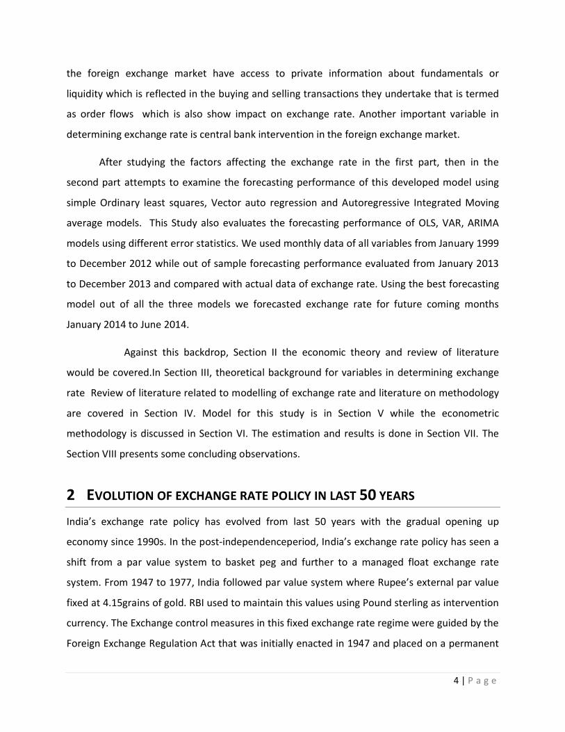
Figure 7.1.3. Autoregressive Distributed Lag results
After overcoming the autocorrelation and unit root problem we left with order flows,
trade balance, money supply, output, forward premium which are significantly affecting
exchange rate. All the variables were significant at 5% level of significance and R-squared value
is greater than 50 percent which means these results are just considerable. Durbin Watson
Statistic confirms that there is no autocorrelation. The variables show same relations as we
expected based on theory that GDP, trade balance with positive sign and order flows, money
supply, forward premium with positive sign. All variables have very small impact on exchange
rate that is 1% change in variables like money supply, trade balance ,order flows show only
0.05 % percent or less change in exchange rate. Only lagged forward premium show 25 %
change in exchange rate.
7.2 RESULTS: FORECASTING OF EXCHANGE RATE
We forecasted exchange rate from January 2013- December 2013 using methods Ordinary
Least Squares (OLS), Vector Auto Regression (VAR), Autoregressive Integrated Moving Average
(ARIMA). We forecasted exchange rate in three samples to see accuracy of forecasting and
then we evaluated the forecasting methods in all these samples by comparing with actual data
of exchange rate. Exchange rate forecasted to 3 months, 6 months, and 12 months ahead from
Dependent Variable: D(EX) Method: Least Squares Date: 04/14/14 Time: 12:23 Sample(adjusted): 1999:03 2013:12 Included observations: 178 after adjusting endpoints
Variable Coefficient Std. Error t-Statistic Prob.
OF(-1) 0.000907 0.000359 2.526698 0.0124 TRB(-1) -4.62E-05 1.56E-05 -2.966825 0.0034
D(MSIND(-1)) 4.61E-07 1.96E-07 2.345309 0.0202 D(GDPIND(-1)) -0.046760 0.017640 -2.650800 0.0088
D(FP(-1)) 0.254382 0.096480 2.636631 0.0091 D(TRB(-1)) -0.000107 3.39E-05 -3.159664 0.0019
R-squared 0.601563 Mean dependent var 0.109028 Adjusted R-squared 0.578353 S.D. dependent var 1.128975 S.E. of regression 1.023356 Akaike info criterion 2.917180 Sum squared resid 180.1285 Schwarz criterion 3.024431 Log likelihood -253.6290 Durbin-Watson stat 1.894235
30 | P a g e
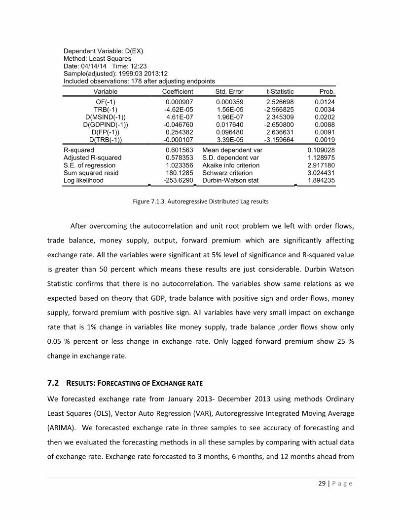
dec-2012. The following figures are forecasting graphs of different methods in three different
samples
Figure 7.2.1. 3-months ahead forecast using different methods
Figure 7.2.2. 6-months ahead forecast using different methods
50
51
52
53
54
55
56
57
2 0 1 2 M 0 9 2 0 1 2 M 1 0 2 0 1 2 M 1 1 2 0 1 2 M 1 2 2 0 1 3 M 0 1 2 0 1 3 M 0 2 2 0 1 3 M 0 3 2 0 1 3 M 0 4 2 0 1 3 M 0 5
3-MONTH AHEAD FORECAST
EX EX_3MNTHSOLS EX_VAR_3M EX_ARIMA_3M
50
52
54
56
58
60
62
64
66
68
6-MONTH AHEAD FORECAST
EX EX_6MNTHSOLS EX_VAR_6MNTHS EX_6M_ARIMA
31 | P a g e
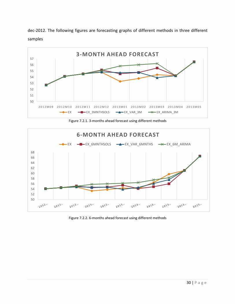
Figure 7.2.3. 12-months ahead forecast using different methods
In all these three figures all these forecasting methods were compared with actual data of
exchange rate. Based on graphs, ARIMA and OLS forecasted data show completely different
pattern from actual data. Especially in 3months and 12 months sample period ARIMA and OLS
graphs shows distinct pattern respectively. Out of all forecasting methods we used we found
that in all the three sample period only VAR shows a similar pattern like actual data. We cannot
say that VAR is best method to forecast the exchange rate but compare to OLS and ARIMA
method VAR is good method to forecast.
Empirically also one can evaluate the performance of forecast of all the three methods
using error statistics. We calculated root mean square error (RMSE) and Theil’s U statistic to
check which method is best in forecasting. The following table gives the values of RMSE and U
statistic for 3 months sample period.
Sample Period for 3- months
Error Statistics OLS VAR ARIMA
Theil’s U statistic 0.008979 0.00827996 0.017449802
RMSE 0.9790815 0.89930765 1.916647719
Table 7.2.1: Error Statistics for OLS, VAR, ARIMA : 3 Month Sample Period
50
55
60
65
70
12-MONTHS AHEAD FORECASTING
EX EX_12MNTHSOLS EX_VAR_12M EX_12M_ARIMA
32 | P a g e
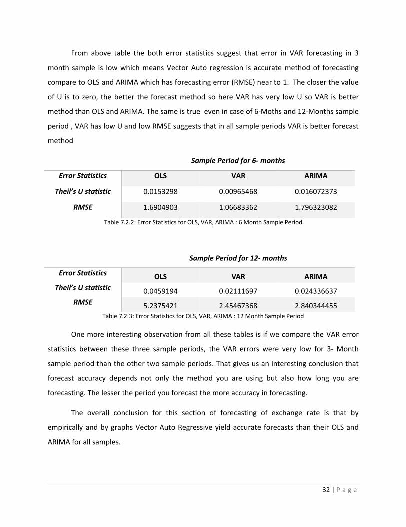
From above table the both error statistics suggest that error in VAR forecasting in 3
month sample is low which means Vector Auto regression is accurate method of forecasting
compare to OLS and ARIMA which has forecasting error (RMSE) near to 1. The closer the value
of U is to zero, the better the forecast method so here VAR has very low U so VAR is better
method than OLS and ARIMA. The same is true even in case of 6-Moths and 12-Months sample
period , VAR has low U and low RMSE suggests that in all sample periods VAR is better forecast
method
Sample Period for 6- months
Error Statistics OLS VAR ARIMA
Theil’s U statistic 0.0153298 0.00965468 0.016072373
RMSE 1.6904903 1.06683362 1.796323082
Table 7.2.2: Error Statistics for OLS, VAR, ARIMA : 6 Month Sample Period
Sample Period for 12- months
Error Statistics OLS VAR ARIMA
Theil’s U statistic 0.0459194 0.02111697 0.024336637
RMSE 5.2375421 2.45467368 2.840344455 Table 7.2.3: Error Statistics for OLS, VAR, ARIMA : 12 Month Sample Period
One more interesting observation from all these tables is if we compare the VAR error
statistics between these three sample periods, the VAR errors were very low for 3- Month
sample period than the other two sample periods. That gives us an interesting conclusion that
forecast accuracy depends not only the method you are using but also how long you are
forecasting. The lesser the period you forecast the more accuracy in forecasting.
The overall conclusion for this section of forecasting of exchange rate is that by
empirically and by graphs Vector Auto Regressive yield accurate forecasts than their OLS and
ARIMA for all samples.

33 | P a g e
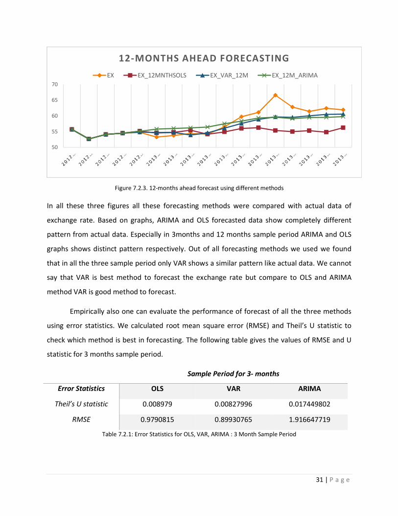
We also forecasted for time period January 2014 to June 2014 out of sample period
using three methods.
Figure 7.2.4. 5-months ahead forecast using different methods (Jan2014- June2014)
Since we concluded that VAR gives accurate forecast so forecast for period Jan 2014- June
2014(Fig.7.2.4) suggest that exchange rate will be fluctuate between 58-60rs per dollar for
coming two months. It is partially true that from January 2014 to May 2014 rupee was
appreciated and settled to below 60 in these months. So, based on this fact in coming May,
June-2014 months the rupee- dollar exchange rate will be around 60rs.
8 CONCLUSIONS
This study covers two main topics: first modelling, where we discussed about the
importance of variables like capital inflows, order flows, central bank intervention in modelling
exchange rate. We empirically estimated the coefficients of explanatory variables after
overcoming autocorrelation and unit root problems. It was found that only variables order flow,
forward premium, trade balance, money supply and output has significant effect on exchange
rate. We also checked for any long term relationship between variables, found that only money
supply and output has long run relationship with exchange rate. All significant variables shows
0
10
20
30
40
50
60
70
0 10 20 30 40 50 60
Forecast for 5 Periods (2014M1-2014M5 ) -- --VAR --- ARIMA .... OLS

34 | P a g e
very small impact on exchange rate except forward premium. Empirical relations between
variables and exchange rate support the theoretical relations.
Second forecasting of exchange rate, we forecasted exchange rate using VAR, OLS,
ARIMA model for three different sample period. Evaluated the forecasting performance of
models by graphs and by error statistics. We found that VAR model yield more accurate
forecasts than the OLS and ARIMA as it has very low Theil’s U and RMSE for all periods. Using
VAR model we also forecasted out of sample for periods from January 2014- June 2014.
9 DATA SOURCES AND ITS DEFINITIONS
Variables Definition Source
EX Rupee/ dollar exchange rate Hand book of statistics on the Indian
Economy and RBI bulletin
GDPIND Index of Industrial Production of India CEIC data source
MSIND Money supply (M3) for India CEIC data source
TRB Trade balance ( export – imports ) RBI Bulletin
CF Capital flows ( FDI +FPI in India ) CEIC data source
OF Purchase – sales of Foreign currency CEIC data source
FP 3-month forward premium
RBII Intervention ( Purchase –sale of US
dollars by RBI)
CEIC data source

35 | P a g e
10 REFERENCES
[1] Dua, Pami, and Rajiv Ranjan. Modeling and Forecasting the Indian RE/US Dollar
Exchange Rate. No. 197. 2011.
[2] Dua, Pami, and Rajiv Ranjan. "Exchange rate policy and modelling in India." OUP
Catalogue (2012).
[3] Dickey, David A., and Wayne A. Fuller. "Distribution of the estimators for autoregressive
time series with a unit root." Journal of the American statistical association 74.366a
(1979): 427-431.
[4] Dua, Pami, and Partha Sen. "Capital Flow Volatility and Exchange Rates: The Case of
India." Delhi School of Economics, Centre for Development Economics, Working
Paper 144 (2006).
[5] Dua, Pami, and Lokendra Kumawat. "Modelling and forecasting seasonality in Indian
macroeconomic time series." Delhi: Centre for Development Economics, Delhi School of
Economics. Working Paper 136 (2005).
[6] Dickey, David A., and Wayne A. Fuller. "Distribution of the estimators for autoregressive
time series with a unit root." Journal of the American statistical association 74.366a
(1979): 427-431.
[7] Dua, Pami, and Partha Sen. "Capital Flow Volatility and Exchange Rates: The Case of
India." Delhi School of Economics, Centre for Development Economics, Working
Paper 144 (2006).
[8] Evans, Martin D., and Richard K. Lyons. "Meese-Rogoff Redux: Micro-based exchange
rate forecasting." CRIF Seminar series. 2005.
[9] Enders, Walter. Applied econometric time series. John Wiley & Sons, 2008.
[10] Feenstra, Robert C. Advanced international trade: theory and evidence. Princeton
University Press, 2003.
[11] Ghatak, Subrata, and Jalal U. Siddiki. "The use of the ARDL approach in estimating virtual
exchange rates in India." Journal of Applied Statistics 28.5 (2001): 573-583.
[12] Goyal, Ashima. "Evolution of India's exchange rate regime." (2012).
[13] Kenen, Peter B. The international economy. Cambridge University Press, 2000.
[14] Long, Dara, and Sovannroeun Samreth. "The monetary model of exchange rate:
evidence from the Philippines using ARDL approach." (2008).
[15] Maddala, Gangadharrao S., and Kajal Lahiri. Introduction to econometrics. Vol. 2. New
York: Macmillan, 1992.
[16] Pesaran, M. Hashem, Yongcheol Shin, and Richard J. Smith. "Bounds testing approaches
to the analysis of level relationships." Journal of applied econometrics16.3 (2001): 289-
326.
[17] Sinha, Pankaj, Sushant Gupta, and Nakul Randev. "MODELING & FORECASTING OF
MACRO-ECONOMIC VARIABLES OF INDIA: BEFORE, DURING & AFTER
RECESSION." Journal of Applied Economic Sciences 6.1 (2011).
36 | P a g e
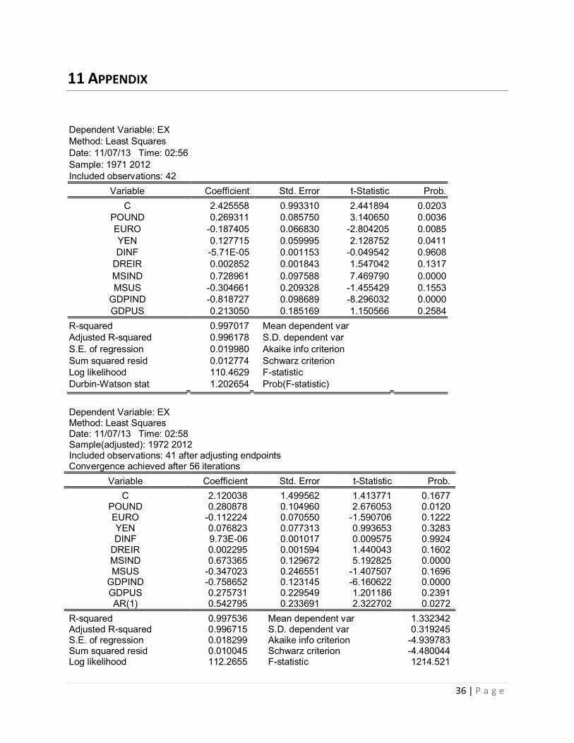
11 APPENDIX
Dependent Variable: EX Method: Least Squares Date: 11/07/13 Time: 02:56 Sample: 1971 2012 Included observations: 42
Variable Coefficient Std. Error t-Statistic Prob.
C 2.425558 0.993310 2.441894 0.0203 POUND 0.269311 0.085750 3.140650 0.0036 EURO -0.187405 0.066830 -2.804205 0.0085 YEN 0.127715 0.059995 2.128752 0.0411 DINF -5.71E-05 0.001153 -0.049542 0.9608
DREIR 0.002852 0.001843 1.547042 0.1317
MSIND 0.728961 0.097588 7.469790 0.0000 MSUS -0.304661 0.209328 -1.455429 0.1553
GDPIND -0.818727 0.098689 -8.296032 0.0000 GDPUS 0.213050 0.185169 1.150566 0.2584
R-squared 0.997017 Mean dependent var Adjusted R-squared 0.996178 S.D. dependent var S.E. of regression 0.019980 Akaike info criterion Sum squared resid 0.012774 Schwarz criterion Log likelihood 110.4629 F-statistic Durbin-Watson stat 1.202654 Prob(F-statistic)
Dependent Variable: EX Method: Least Squares Date: 11/07/13 Time: 02:58 Sample(adjusted): 1972 2012 Included observations: 41 after adjusting endpoints Convergence achieved after 56 iterations
Variable Coefficient Std. Error t-Statistic Prob.
C 2.120038 1.499562 1.413771 0.1677 POUND 0.280878 0.104960 2.676053 0.0120 EURO -0.112224 0.070550 -1.590706 0.1222 YEN 0.076823 0.077313 0.993653 0.3283 DINF 9.73E-06 0.001017 0.009575 0.9924
DREIR 0.002295 0.001594 1.440043 0.1602 MSIND 0.673365 0.129672 5.192825 0.0000 MSUS -0.347023 0.246551 -1.407507 0.1696
GDPIND -0.758652 0.123145 -6.160622 0.0000 GDPUS 0.275731 0.229549 1.201186 0.2391 AR(1) 0.542795 0.233691 2.322702 0.0272
R-squared 0.997536 Mean dependent var 1.332342 Adjusted R-squared 0.996715 S.D. dependent var 0.319245 S.E. of regression 0.018299 Akaike info criterion -4.939783 Sum squared resid 0.010045 Schwarz criterion -4.480044 Log likelihood 112.2655 F-statistic 1214.521

37 | P a g e
Durbin-Watson stat 1.775138 Prob(F-statistic) 0.000000
Unit root tests for variables
EX- I1 Null Hypothesis: D(EX) has a unit root Exogenous: Constant, Linear Trend Lag Length: 0 (Automatic - based on SIC, maxlag=9)
t-Statistic Prob.* Augmented Dickey-Fuller test statistic -4.229308 0.0094
Test critical values: 1% level -4.205004 5% level -3.526609 10% level -3.194611 *MacKinnon (1996) one-sided p-values.
Augmented Dickey-Fuller Test Equation Dependent Variable: D(EX,2) Method: Least Squares Date: 07/11/13 Time: 22:45 Sample (adjusted): 1973 2012 Included observations: 40 after adjustments
Variable Coefficient Std. Error t-Statistic Prob. D(EX(-1)) -0.666578 0.157609 -4.229308 0.0001
C 0.016280 0.011726 1.388291 0.1734 @TREND(1971) -8.10E-05 0.000453 -0.179053 0.8589
R-squared 0.326432 Mean dependent var 0.001089
Adjusted R-squared 0.290022 S.D. dependent var 0.039043 S.E. of regression 0.032897 Akaike info criterion -3.918809 Sum squared resid 0.040043 Schwarz criterion -3.792143 Log likelihood 81.37619 Hannan-Quinn criter. -3.873011 F-statistic 8.965657 Durbin-Watson stat 1.972901 Prob(F-statistic) 0.000668
Pound – I2 Null Hypothesis: D(POUND,2) has a unit root Exogenous: Constant, Linear Trend Lag Length: 0 (Automatic - based on SIC, maxlag=8)
t-Statistic Prob.* Augmented Dickey-Fuller test statistic -5.900016 0.0001
Test critical values: 1% level -4.211868 5% level -3.529758 10% level -3.196411 *MacKinnon (1996) one-sided p-values.
Augmented Dickey-Fuller Test Equation Dependent Variable: D(POUND,3) Method: Least Squares
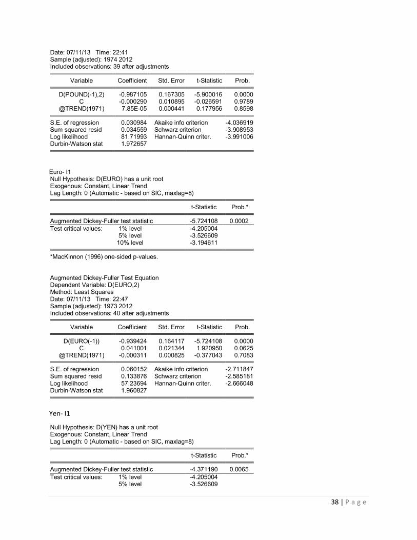
38 | P a g e
Date: 07/11/13 Time: 22:41 Sample (adjusted): 1974 2012 Included observations: 39 after adjustments
Variable Coefficient Std. Error t-Statistic Prob. D(POUND(-1),2) -0.987105 0.167305 -5.900016 0.0000
C -0.000290 0.010895 -0.026591 0.9789 @TREND(1971) 7.85E-05 0.000441 0.177956 0.8598
S.E. of regression 0.030984 Akaike info criterion -4.036919
Sum squared resid 0.034559 Schwarz criterion -3.908953 Log likelihood 81.71993 Hannan-Quinn criter. -3.991006 Durbin-Watson stat 1.972657
Euro- I1 Null Hypothesis: D(EURO) has a unit root Exogenous: Constant, Linear Trend Lag Length: 0 (Automatic - based on SIC, maxlag=8)
t-Statistic Prob.* Augmented Dickey-Fuller test statistic -5.724108 0.0002
Test critical values: 1% level -4.205004 5% level -3.526609 10% level -3.194611 *MacKinnon (1996) one-sided p-values.
Augmented Dickey-Fuller Test Equation Dependent Variable: D(EURO,2) Method: Least Squares Date: 07/11/13 Time: 22:47 Sample (adjusted): 1973 2012 Included observations: 40 after adjustments
Variable Coefficient Std. Error t-Statistic Prob. D(EURO(-1)) -0.939424 0.164117 -5.724108 0.0000
C 0.041001 0.021344 1.920950 0.0625 @TREND(1971) -0.000311 0.000825 -0.377043 0.7083
S.E. of regression 0.060152 Akaike info criterion -2.711847
Sum squared resid 0.133876 Schwarz criterion -2.585181 Log likelihood 57.23694 Hannan-Quinn criter. -2.666048 Durbin-Watson stat 1.960827
Yen- I1
Null Hypothesis: D(YEN) has a unit root Exogenous: Constant, Linear Trend Lag Length: 0 (Automatic - based on SIC, maxlag=8)
t-Statistic Prob.* Augmented Dickey-Fuller test statistic -4.371190 0.0065
Test critical values: 1% level -4.205004 5% level -3.526609

39 | P a g e
10% level -3.194611 *MacKinnon (1996) one-sided p-values.
Augmented Dickey-Fuller Test Equation Dependent Variable: D(YEN,2) Method: Least Squares Date: 07/11/13 Time: 22:48 Sample (adjusted): 1973 2012 Included observations: 40 after adjustments
Variable Coefficient Std. Error t-Statistic Prob. D(YEN(-1)) -0.684751 0.156651 -4.371190 0.0001
C 0.025000 0.017264 1.448107 0.1560 @TREND(1971) -5.92E-05 0.000659 -0.089784 0.9289
S.E. of regression 0.047988 Akaike info criterion -3.163706
Sum squared resid 0.085204 Schwarz criterion -3.037040 Log likelihood 66.27411 Hannan-Quinn criter. -3.117907 Durbin-Watson stat 2.010957
DINf- I0
Null Hypothesis: DINF has a unit root Exogenous: Constant Lag Length: 0 (Automatic - based on SIC, maxlag=9)
t-Statistic Prob.* Augmented Dickey-Fuller test statistic -4.592507 0.0006
Test critical values: 1% level -3.600987 5% level -2.935001 10% level -2.605836 *MacKinnon (1996) one-sided p-values.
Augmented Dickey-Fuller Test Equation Dependent Variable: D(DINF) Method: Least Squares Date: 07/11/13 Time: 22:50 Sample (adjusted): 1972 2012 Included observations: 41 after adjustments
Variable Coefficient Std. Error t-Statistic Prob. DINF(-1) -0.693663 0.151042 -4.592507 0.0000
C 2.878034 0.843916 3.410332 0.0015 R-squared 0.350986 Mean dependent var 0.132867
Adjusted R-squared 0.334344 S.D. dependent var 4.675350 S.E. of regression 3.814512 Akaike info criterion 5.563053 Sum squared resid 567.4696 Schwarz criterion 5.646642 Log likelihood -112.0426 Hannan-Quinn criter. 5.593492 F-statistic 21.09112 Durbin-Watson stat 1.913406 Prob(F-statistic) 0.000045

40 | P a g e
DREIR- I0
Null Hypothesis: DREIR has a unit root Exogenous: Constant Lag Length: 0 (Automatic - based on SIC, maxlag=9)
t-Statistic Prob.* Augmented Dickey-Fuller test statistic -4.869044 0.0003
Test critical values: 1% level -3.600987 5% level -2.935001 10% level -2.605836 *MacKinnon (1996) one-sided p-values.
Augmented Dickey-Fuller Test Equation Dependent Variable: D(DREIR) Method: Least Squares Date: 07/11/13 Time: 22:51 Sample (adjusted): 1972 2012 Included observations: 41 after adjustments
Variable Coefficient Std. Error t-Statistic Prob. DREIR(-1) -0.755179 0.155098 -4.869044 0.0000
C 1.190176 0.481055 2.474097 0.0178 R-squared 0.378066 Mean dependent var 0.014772
Adjusted R-squared 0.362119 S.D. dependent var 3.335941 S.E. of regression 2.664331 Akaike info criterion 4.845334 Sum squared resid 276.8478 Schwarz criterion 4.928923 Log likelihood -97.32935 Hannan-Quinn criter. 4.875772 F-statistic 23.70759 Durbin-Watson stat 2.042907 Prob(F-statistic) 0.000019
MSIND-I1
Null Hypothesis: D(MSIND) has a unit root Exogenous: Constant Lag Length: 0 (Automatic - based on SIC, maxlag=9)
t-Statistic Prob.* Augmented Dickey-Fuller test statistic -5.360588 0.0001
Test critical values: 1% level -3.605593 5% level -2.936942 10% level -2.606857 *MacKinnon (1996) one-sided p-values.
Augmented Dickey-Fuller Test Equation Dependent Variable: D(MSIND,2) Method: Least Squares Date: 07/11/13 Time: 22:52 Sample (adjusted): 1973 2012 Included observations: 40 after adjustments
Variable Coefficient Std. Error t-Statistic Prob.

41 | P a g e
D(MSIND(-1)) -0.924860 0.172530 -5.360588 0.0000 C 0.063615 0.012060 5.274965 0.0000 R-squared 0.430591 Mean dependent var -0.000417
Adjusted R-squared 0.415607 S.D. dependent var 0.013735 S.E. of regression 0.010500 Akaike info criterion -6.226148 Sum squared resid 0.004190 Schwarz criterion -6.141704 Log likelihood 126.5230 Hannan-Quinn criter. -6.195616 F-statistic 28.73591 Durbin-Watson stat 1.830099 Prob(F-statistic) 0.000004
MSUS-I2
Null Hypothesis: D(MSUS,2) has a unit root Exogenous: Constant, Linear Trend Lag Length: 0 (Automatic - based on SIC, maxlag=6)
t-Statistic Prob.* Augmented Dickey-Fuller test statistic -6.021815 0.0001
Test critical values: 1% level -4.211868 5% level -3.529758 10% level -3.196411 *MacKinnon (1996) one-sided p-values.
Augmented Dickey-Fuller Test Equation Dependent Variable: D(MSUS,3) Method: Least Squares Date: 07/11/13 Time: 22:54 Sample (adjusted): 1974 2012 Included observations: 39 after adjustments
Variable Coefficient Std. Error t-Statistic Prob. D(MSUS(-1),2) -0.994513 0.165152 -6.021815 0.0000
C -0.001779 0.004693 -0.379109 0.7068 @TREND(1971) 7.37E-05 0.000190 0.388526 0.6999
S.E. of regression 0.013273 Akaike info criterion -5.732357
Sum squared resid 0.006342 Schwarz criterion -5.604391 Log likelihood 114.7810 Hannan-Quinn criter. -5.686444 Durbin-Watson stat 2.015565
GDPIND- I1
Null Hypothesis: D(GDPIND) has a unit root Exogenous: Constant, Linear Trend Lag Length: 0 (Automatic - based on SIC, maxlag=7)
t-Statistic Prob.* Augmented Dickey-Fuller test statistic -5.733226 0.0001
Test critical values: 1% level -4.205004 5% level -3.526609 10% level -3.194611 *MacKinnon (1996) one-sided p-values.

42 | P a g e
Augmented Dickey-Fuller Test Equation Dependent Variable: D(GDPIND,2) Method: Least Squares Date: 07/11/13 Time: 22:55 Sample (adjusted): 1973 2012 Included observations: 40 after adjustments
Variable Coefficient Std. Error t-Statistic Prob. D(GDPIND(-1)) -0.959427 0.167345 -5.733226 0.0000
C 0.030323 0.012920 2.346881 0.0244 @TREND(1971) 0.000154 0.000496 0.311137 0.7574
S.E. of regression 0.035945 Akaike info criterion -3.741611
Sum squared resid 0.047806 Schwarz criterion -3.614945 Log likelihood 77.83222 Hannan-Quinn criter. -3.695813 Durbin-Watson stat 1.917953
GDPUS-I1 Null Hypothesis: D(GDPUS) has a unit root Exogenous: Constant, Linear Trend Lag Length: 0 (Automatic - based on SIC, maxlag=5)
t-Statistic Prob.* Augmented Dickey-Fuller test statistic -5.060891 0.0010
Test critical values: 1% level -4.205004 5% level -3.526609 10% level -3.194611 *MacKinnon (1996) one-sided p-values.
Augmented Dickey-Fuller Test Equation Dependent Variable: D(GDPUS,2) Method: Least Squares Date: 07/11/13 Time: 22:58 Sample (adjusted): 1973 2012 Included observations: 40 after adjustments
Variable Coefficient Std. Error t-Statistic Prob. D(GDPUS(-1)) -0.821875 0.162397 -5.060891 0.0000
C 0.037508 0.008084 4.639766 0.0000 @TREND(1971) -0.000691 0.000181 -3.828381 0.0005
S.E. of regression 0.008479 Akaike info criterion -6.630361
Sum squared resid 0.002660 Schwarz criterion -6.503696 Log likelihood 135.6072 Hannan-Quinn criter. -6.584563 Durbin-Watson stat 1.920272
Dependent Variable: EX

43 | P a g e
Method: Least Squares Date: 04/14/14 Time: 12:32 Sample(adjusted): 2004:10 2012:12 Included observations: 99 after adjusting endpoints
Variable Coefficient Std. Error t-Statistic Prob.
C 58.26540 3.511630 16.59212 0.0000 MSIND 5.06E-07 6.52E-08 7.762642 0.0000 GDPIND -0.247175 0.047815 -5.169447 0.0000 CF -0.000561 0.000231 -2.435048 0.0168 OF -0.002259 0.000969 -2.330536 0.0220 FP -0.018669 0.180980 -0.103156 0.9181 TRB 0.000135 9.20E-05 1.464469 0.1465 RBII -0.000214 6.21E-05 -3.451817 0.0008
R-squared 0.710616 Mean dependent var 46.09847 Adjusted R-squared 0.688355 S.D. dependent var 4.023093 S.E. of regression 2.245898 Akaike info criterion 4.533444 Sum squared resid 459.0092 Schwarz criterion 4.743150 Log likelihood -216.4055 F-statistic 31.92295 Durbin-Watson stat 0.672714 Prob(F-statistic) 0.000000
Dependent Variable: EX Method: Least Squares Date: 04/12/14 Time: 23:11 Sample (adjusted): 2004M11 2012M12 Included observations: 98 after adjustments Convergence achieved after 28 iterations
Variable Coefficient Std. Error t-Statistic Prob. C 34.06170 5.072725 6.714675 0.0000
MSIND 2.16E-07 8.36E-08 2.579553 0.0115 GDPIND 0.030345 0.025692 1.181100 0.2407
CF -0.000174 0.000112 -1.558787 0.1226 OF -0.001430 0.000514 -2.782253 0.0066 FP -0.368885 0.137225 -2.688173 0.0086
TRB 8.83E-05 4.47E-05 1.974677 0.0514 RBII -6.17E-05 2.89E-05 -2.137524 0.0353
AR(1) 0.927394 0.038846 23.87337 0.0000 R-squared 0.934178 Mean dependent var 46.10509
Adjusted R-squared 0.928262 S.D. dependent var 4.043236 S.E. of regression 1.082939 Akaike info criterion 3.084577 Sum squared resid 104.3754 Schwarz criterion 3.321972 Log likelihood -142.1443 Hannan-Quinn criter. 3.180599 F-statistic 157.8925 Durbin-Watson stat 1.622126 Prob(F-statistic) 0.000000
Inverted AR Roots .93

44 | P a g e
d(ex) c msind gdpind cf of fp trb rbii ar(1) ma(1)
Dependent Variable: D(EX) Method: Least Squares Date: 04/13/14 Time: 00:56 Sample (adjusted): 2004M11 2012M12 Included observations: 98 after adjustments Convergence achieved after 40 iterations MA Backcast: 2004M10
Variable Coefficient Std. Error t-Statistic Prob. C -0.731625 1.848021 -0.395896 0.6931
MSIND 2.85E-09 3.45E-08 0.082504 0.9344 GDPIND 0.007266 0.024965 0.291027 0.7717
CF -4.57E-05 0.000118 -0.388353 0.6987 OF -0.001801 0.000503 -3.576961 0.0006 FP -0.192543 0.098743 -1.949943 0.0544
TRB -4.51E-05 4.81E-05 -0.937057 0.3513 RBII -3.12E-07 3.09E-05 -0.010095 0.9920
AR(1) -0.538002 0.259759 -2.071158 0.0413 MA(1) 0.743377 0.206441 3.600916 0.0005
R-squared 0.283665 Mean dependent var 0.095173
Adjusted R-squared 0.210404 S.D. dependent var 1.230245 S.E. of regression 1.093186 Akaike info criterion 3.112521 Sum squared resid 105.1650 Schwarz criterion 3.376294 Log likelihood -142.5135 Hannan-Quinn criter. 3.219212 F-statistic 3.871956 Durbin-Watson stat 2.050198 Prob(F-statistic) 0.000363
Inverted AR Roots -.54
Inverted MA Roots -.74
d(ex) ex(-1) msind(-1) gdpind(-1) cf(-1) of(-1) fp(-1) trb(-1) rbii(-1) d(ex(-1)) d(msind(-1)) d(gdpind(-1))
d(cf(-1)) d(of(-1)) d(fp(-1)) d(trb(-1)) d(rbii(-1))
Dependent Variable: D(EX) Method: Least Squares Date: 04/14/14 Time: 12:53 Sample(adjusted): 1999:03 2013:12 Included observations: 178 after adjusting endpoints
Variable Coefficient Std. Error t-Statistic Prob.
EX(-1) -3.88E-05 0.014666 -0.002647 0.9979 MSIND(-1) -8.83E-09 1.30E-08 -0.678297 0.4985
GDPIND(-1) -0.000752 0.009198 -0.081717 0.9350 OF(-1) -0.000563 0.000530 -1.061307 0.2901 FP(-1) 0.044751 0.049021 0.912891 0.3626
TRB(-1) -7.75E-05 4.97E-05 -1.560076 0.1207 RBII(-1) 9.51E-06 3.89E-05 0.244808 0.8069
D(EX(-1)) 0.005232 0.086148 0.060730 0.9516 D(MSIND(-1)) -3.48E-07 2.39E-07 -1.453006 0.1481
D(GDPIND(-1)) -0.052070 0.019908 -2.615498 0.0097 D(OF(-1)) -0.000872 0.000564 -1.545516 0.1241

45 | P a g e
D(FP(-1)) -0.216391 0.107981 -2.003969 0.0467 D(TRB(-1)) -6.79E-05 4.65E-05 -1.459167 0.1464 D(RBII(-1)) -1.85E-05 3.07E-05 -0.601586 0.5483
R-squared 0.225982 Mean dependent var 0.109028 Adjusted R-squared 0.164627 S.D. dependent var 1.128975 S.E. of regression 1.031869 Akaike info criterion 2.976006 Sum squared resid 174.6195 Schwarz criterion 3.226259 Log likelihood -250.8646 Durbin-Watson stat 1.995937
Dependent Variable: D(EX) Dependent Variable: D(EX) Method: Least Squares Date: 04/14/14 Time: 12:53 Sample(adjusted): 1999:03 2013:12 Included observations: 178 after adjusting endpoints
Variable Coefficient Std. Error t-Statistic Prob.
EX(-1) -3.88E-05 0.014666 -0.002647 0.9979 MSIND(-1) -8.83E-09 1.30E-08 -0.678297 0.4985
GDPIND(-1) -0.000752 0.009198 -0.081717 0.9350 OF(-1) -0.000563 0.000530 -1.061307 0.2901 FP(-1) 0.044751 0.049021 0.912891 0.3626
TRB(-1) -7.75E-05 4.97E-05 -1.560076 0.1207 RBII(-1) 9.51E-06 3.89E-05 0.244808 0.8069
D(EX(-1)) 0.005232 0.086148 0.060730 0.9516 D(MSIND(-1)) -3.48E-07 2.39E-07 -1.453006 0.1481
D(GDPIND(-1)) -0.052070 0.019908 -2.615498 0.0097 D(OF(-1)) -0.000872 0.000564 -1.545516 0.1241 D(FP(-1)) -0.216391 0.107981 -2.003969 0.0467
D(TRB(-1)) -6.79E-05 4.65E-05 -1.459167 0.1464 D(RBII(-1)) -1.85E-05 3.07E-05 -0.601586 0.5483
R-squared 0.225982 Mean dependent var 0.109028 Adjusted R-squared 0.164627 S.D. dependent var 1.128975 S.E. of regression 1.031869 Akaike info criterion 2.976006 Sum squared resid 174.6195 Schwarz criterion 3.226259 Log likelihood -250.8646 Durbin-Watson stat 1.995937
Forecast: EXF_3M_OLS Actual: EX Forecast sample: 2012M12 2013M03 Included observations: 4
Root Mean Squared Error 0.979081
Mean Absolute Error 0.922068 Mean Absolute Percentage Error 1.711053 Theil Inequality Coefficient 0.008979 Bias Proportion 0.886928 Variance Proportion 0.044332 Covariance Proportion 0.068740