Modelling for Engineering& Human Behaviour 2020

Valencia, 8− 10 July 2020

This book includes the extended abstracts of papers presented at XXII Edition of the Mathe-matical Modelling Conference Series at the Institute for Multidisciplinary Mathematics “Math-ematical Modelling in Engineering & Human Behaviour”.

I.S.B.N.: 978-84-09-25132-2Version: 10-11-2020Report any problems with this document to ellona1@upvnet.upv.es.

Edited by: R. Company, J. C. Cortes, L. Jodar and E. Lopez-Navarro.Credits: The cover has been designed using images from kjpargeter/freepik.

This book has been supported by the EuropeanUnion through the Operational Program of the [Eu-ropean Regional Development Fund (ERDF) / Eu-ropean Social Fund (ESF)] of the Valencian Com-munity 2014-2020. [Record: GJIDI/2018/A/010].

Contents

Dopamine imbalance: A systemic approach to diseases and treatments, bySalvador Amigo.. . . . . . . . . . . . . . . . . . . . . . . . . . . . . . . . . . . . . . . . . . . . . . . . . . . . . . . . . . . . . . . . . . . . . . . . . . .1

New solution for automatic and real time detection of railroad switch fail-ures and diagnosis, by Jorge del Pozo, Laura Andres, Rafael Femenıa and Laura Rubio. . . . . . . . . .8

An integrated model to optimize Berth Allocation Problem and Yard Plan-ner, by C. Burgos, J.C. Cortes, D. Martınez-Rodrıguez, J. Villanueva-Oller and R.J. Villanueva. . . . . .12

Dynamical analysis of a new three-step class of iterative methods for solvingnonlinear systems, by Raudys R. Capdevila, Alicia Cordero and Juan R. Torregrosa. . . . . . . . . . . 19

Integrating the human factor in FMECA-based risk evaluation throughBayesian networks, by S. Carpitella, J. Izquierdo, M. Plajner and J. Vomlel. . . . . . . . . . . . . . . . . . 24

Stable positive Monte Carlo finite difference techniques for random parabolicpartial differential equations, by M.-C. Casaban, R. Company and L. Jodar. . . . . . . . . . . . . . . 30

Invariant energy in short-term personality dynamics, by Antonio Caselles, SalvadorAmigo and Joan C. Mico. . . . . . . . . . . . . . . . . . . . . . . . . . . . . . . . . . . . . . . . . . . . . . . . . . . . . . . . . . . . . . . . . . .36

Suitable approximations for the self-accelerating parameters in iterativemethods with memory, by F. I. Chicharro, N. Garrido, A. Cordero and J.R. Torregrosa. . . . . . . 42

Predictive maintenance system for a dam based on real-time monitoringand diagnosis, by Ernesto Colomer, Carlos Canales, Jesus Terradez and Salvador Mateo. . . . . . . . . 48

Approximating the matrix hyperbolic tangent, by Emilio Defez, Jose Miguel Alonso,Javier Ibanez, Pedro Alonso-Jorda and Jorge Sastre. . . . . . . . . . . . . . . . . . . . . . . . . . . . . . . . . . . . . . . . . . . . 52

Efficient finite element modelling of sound propagation in after-treatmentdevices with arbitrary cross section, by F.D. Denia, E.M. Sanchez-Orgaz, B. Ferrandiz, J.Martınez-Casas and L. Baeza. . . . . . . . . . . . . . . . . . . . . . . . . . . . . . . . . . . . . . . . . . . . . . . . . . . . . . . . . . . . . . . 59

Iterative algorithms for computing generalized inverses, by A. Cordero, N. Garrido,P. Soto-Quiros and J.R. Torregrosa. . . . . . . . . . . . . . . . . . . . . . . . . . . . . . . . . . . . . . . . . . . . . . . . . . . . . . . . . . 66

Communities’ detection in weakly connected directed graphs, by J. M. Montanana,A. Hervas and P. P. Soriano. . . . . . . . . . . . . . . . . . . . . . . . . . . . . . . . . . . . . . . . . . . . . . . . . . . . . . . . . . . . . . . . 72

Comparison in the use of ANSYS and SAP2000 in the modelling and struc-tural calculation of bridges, by Miriam Labrado, Ernesto Colomer, Adrian Zornoza and AlvaroPotti. . . . . . . . . . . . . . . . . . . . . . . . . . . . . . . . . . . . . . . . . . . . . . . . . . . . . . . . . . . . . . . . . . . . . . . . . . . . . . . . . . . .78

iv

Modelling for Engineering & Human Behaviour 2020

Analysing nonlinear oscillators subject to Gaussian inputs via the randomperturbation technique, by J.-C. Cortes, E. Lopez-Navarro, J.-V. Romero and M.-D. Rosello. . 82

A note on the use the semifocal anomaly as temporal variable in the twobody problem, by Jose Antonio Lopez Ortı, Francisco Jose Marco Castillo and Marıa Jose MartınezUso. . . . . . . . . . . . . . . . . . . . . . . . . . . . . . . . . . . . . . . . . . . . . . . . . . . . . . . . . . . . . . . . . . . . . . . . . . . . . . . . . . . . .87

Epidemiological modelling of COVID-19 in Granada, Spain: Analysis offuture scenarios, by Jose-Manuel Garrido, David Martınez-Rodrıguez, Fernando Rodrıguez-Serrano,Raul S-Julian and Rafael-J. Villanueva. . . . . . . . . . . . . . . . . . . . . . . . . . . . . . . . . . . . . . . . . . . . . . . . . . . . . . . 91

Probabilistic calibration of a model of herpes simplex type 2 with a prefixederror in the uncertainty of the data, by Juan-Carlos Cortes, Pablo Martınez-Rodrıguez, Jose-A. Morano, Jose-Vicente Romero, Marıa-Dolores Rosello and Rafael-J. Villanueva. . . . . . . . . . . . . . . . . . 96

A proposal for quantum short time personality dynamics, by Joan C. Mico,Salvador Amigo and Antonio Caselles. . . . . . . . . . . . . . . . . . . . . . . . . . . . . . . . . . . . . . . . . . . . . . . . . . . . . . . 102

Energy footprint reduction of Chile’s social interest homes: an integer linearprogramming approach, by Felipe Monsalve and David Soler. . . . . . . . . . . . . . . . . . . . . . . . . . . . 109

Statistical solution of a second-order chemical reaction, by J.-C. Cortes, A.Navarro-Quiles, J.-V. Romero and M.-D. Rosello. . . . . . . . . . . . . . . . . . . . . . . . . . . . . . . . . . . . . . . . . . . . . . . . . . . . . 115

On comparing Spotify Top 200 lists, by F. Pedroche and J. A. Conejero. . . . . . . . . . . . .121

New autonomous system for slope stability control in linear infrastructure,by Alvaro Potti, Gonzalo Munielo, Julian Santos and Jordi Marco. . . . . . . . . . . . . . . . . . . . . . . . . . . . . . . 125

Application of a twin model for monitoring and predictive diagnosis ofPirihueico Bridge, by Marcelo Marquez, Francisca Espinoza, Sandra Achurra, Julia Real, ErnestoColomer and Miriam Labrado. . . . . . . . . . . . . . . . . . . . . . . . . . . . . . . . . . . . . . . . . . . . . . . . . . . . . . . . . . . . . 129

N-soft set based multi-agent decisions: A decide-then-merge strategy, byJ.C.R. Alcantud, G. Santos-Garcıa and M. Akram. . . . . . . . . . . . . . . . . . . . . . . . . . . . . . . . . . . . . . . . . . . . 133

Deep Learning AI-based solution for vineyard real-time health monitoring,by Ana Sancho, Eliseo Gomez, Albert Perez and Julian Santos. . . . . . . . . . . . . . . . . . . . . . . . . . . . . . . . . .138

New system for the automatic counting of vehicles in roundabouts andintersections, by Teresa Real, Ruben Sancho, Guillem Alandı and Fernando Lopez. . . . . . . . . . . . . 142

A System Dynamics model to predict the impact of COVID-19 in Spain, byM.T. Sanz, A. Caselles, J. C. Mico and C. Soler. . . . . . . . . . . . . . . . . . . . . . . . . . . . . . . . . . . . . . . . . . . . . . 146

An epidemic grid model to address the spread of Covid-19. The case ofValencian Community (Spain), by M.T Signes Pont, J.J. Cortes Plana, H. Mora Mora and C.Bordehore Fontanet. . . . . . . . . . . . . . . . . . . . . . . . . . . . . . . . . . . . . . . . . . . . . . . . . . . . . . . . . . . . . . . . . . . . . . 152

The Relativistic Harmonic Oscillator in a Uniform Gravitational Field, byMichael M. Tung. . . . . . . . . . . . . . . . . . . . . . . . . . . . . . . . . . . . . . . . . . . . . . . . . . . . . . . . . . . . . . . . . . . . . . . . 157

A disruptive technology that enables low cost real-time monitoring of roadpavement condition by any ordinary vehicle circulating on the road, and au-tomatically designs plans for predictive maintenance, by Francisco Jose Vea, AdrianZornoza, Juan Ramon Sanchez and Ismael Munoz. . . . . . . . . . . . . . . . . . . . . . . . . . . . . . . . . . . . . . . . . . . . 163

v

Approximating the matrix hyperbolic tangent

Emilio Defez[1, Jose Miguel Alonso\, Javier Ibanez\, Pedro Alonso-Jorda] and Jorge Sastre†

([) Instituto de Matematica Multidisciplinar,Camino de Vera s/n, 46022, Valencia, Spain,

(\) Instituto de Instrumentacion para Imagen Molecular,Camino de Vera s/n, 46022, Valencia, Spain,

(]) Grupo Interdisciplinar de Computacion y Comunicaciones,Camino de Vera s/n, 46022, Valencia, Spain,

(†) Instituto de Telecomunicacion y Aplicaciones Multimedia,Camino de Vera s/n, 46022, Valencia, Spain.

1 Introduction. On hyperbolic matrix functionsOur objective is to find approximations of the hyperbolic tangent matrix function tanh(A), A ∈Cn×n, defined as:

tanh (A) = sinh (A) (cosh (A))−1 = (cosh (A))−1 sinh (A), (1)

wherecosh (A) = 1

2(eA + e−A

), sinh (A) = 1

2(eA − e−A

)(2)

are defined in terms of the exponential matrix eA. The hyperbolic tangent matrix function isused to give an analytical solution of the radiative transfer equation [1], in the study of calortransference [2, 3], in the study of symplectic systems [4, 5] or in graph theory [6].

In this work, we are going to focus on the study of two methods to compute the hyperbolictangent matrix function tanh (A).

Method based on the exponential matrix. This method is based on the definition (2)and formula (1), from which the following matrix rational expression is immediately deduced:

tanh (A) =(e2A − I

) (e2A + I

)−1=(e2A + I

)−1 (e2A − I

), (3)

where I denotes the identity matrix with the same dimension as A. Expression (3) reduces theapproximation of the hyperbolic tangent matrix function to the approximation of the exponen-tial matrix e2A. There are profuse and well known literature about the approximation of thismatrix function. In general, the most competitive methods used in practice are those basedon polynomial approximations and on Pade rational approximations, where the first methods

1e-mail: edefez@imm.upv.es

52

Modelling for Engineering & Human Behaviour 2020

are generally more accurate and with less computational cost. There are different polynomialapproximations of the exponential matrix based on distinct classes of matrix polynomials suchas Taylor, see reference [7] for example, or Hermite, see reference [8]. Recently, a method basedon Bernoulli matrix polynomials has been proposed in [9].

All these methods use the scaling and squaring technique. This technique is based on iden-tity eA =

(e2−sA

)2sthat satisfies the matrix exponential. In the scaling phase, an integer scaling

factor s is taking and the approximation of e2−sA is made using any of the proposed methodsso that the required precision is obtained with the lowest possible computational cost. In thesquaring phase, we obtain eA by s repeated squaring.

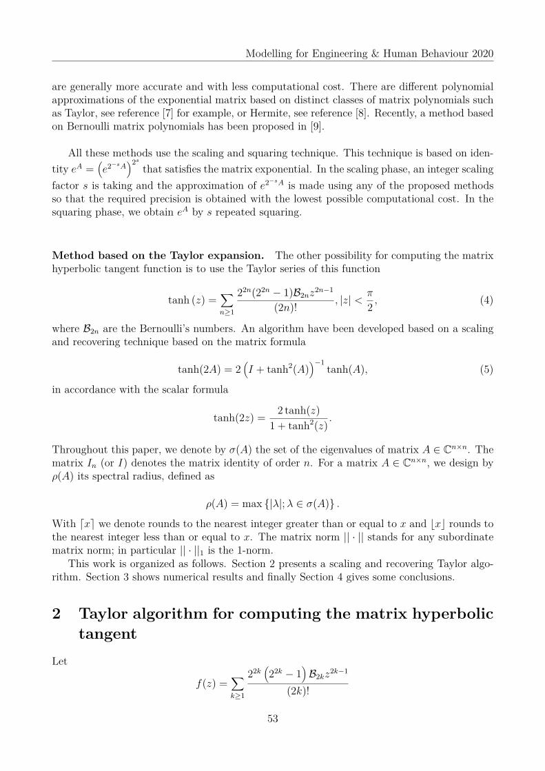
Method based on the Taylor expansion. The other possibility for computing the matrixhyperbolic tangent function is to use the Taylor series of this function

tanh (z) =∑n≥1

22n(22n − 1)B2nz2n−1

(2n)! , |z| < π

2 , (4)

where B2n are the Bernoulli’s numbers. An algorithm have been developed based on a scalingand recovering technique based on the matrix formula

tanh(2A) = 2(I + tanh2(A)

)−1tanh(A), (5)

in accordance with the scalar formula

tanh(2z) = 2 tanh(z)1 + tanh2(z)

.

Throughout this paper, we denote by σ(A) the set of the eigenvalues of matrix A ∈ Cn×n. Thematrix In (or I) denotes the matrix identity of order n. For a matrix A ∈ Cn×n, we design byρ(A) its spectral radius, defined as

ρ(A) = max {|λ|;λ ∈ σ(A)} .

With dxe we denote rounds to the nearest integer greater than or equal to x and bxc rounds tothe nearest integer less than or equal to x. The matrix norm || · || stands for any subordinatematrix norm; in particular || · ||1 is the 1-norm.

This work is organized as follows. Section 2 presents a scaling and recovering Taylor algo-rithm. Section 3 shows numerical results and finally Section 4 gives some conclusions.

2 Taylor algorithm for computing the matrix hyperbolictangent

Let

f(z) =∑k≥1

22k(22k − 1

)B2kz

2k−1

(2k)!

53

Modelling for Engineering & Human Behaviour 2020

be the Taylor series expansion of the hyperbolic tangent function, with radius of convergencer = π/2. The matrix hyperbolic tangent can be defined for all A ∈ Cn×n by the series

f(A) =∑k≥1

22k(22k − 1

)B2kA

2k−1

(2k)! , ρ(A) < π/2 (6)

where B2n are the Bernoulli’s numbers, defined by recursive expression

B0 = 1 , Bk = −k−1∑i=0

(k

i

)Bi

k + 1− i , k ≥ 1. (7)

To simplify the notation, we denote with

tanh(A) =∑k≥0

q2k+1A2k+1

the series expansions (6) and with

T2m+1(A) =m∑k=0

q2k+1A2k+1 = A

m∑k=0

pkBk = APm(B) (8)

the Taylor approximation of order 2m+ 1 of tanh(A), where B = A2.

In the Paterson-Stockmeyer method, see [10], an integer mk is chosen from the set

M = {2, 4, 6, 9, 12, 16, 20, 25, 30, . . . } ,

and the powers Bi, 2 ≤ i ≤ q, are calculated, where q =⌈√

mk

⌉or q = b√mkc, such that

Pmk(B) = (9)(((pmkBq + pmk−1B

q−1 + pmk−2Bq−2 + · · ·+ pmk−q+1B + pmk−qI)Bq

+ pmk−q−1Bq−1 + pmk−q−2B

q−2 + · · ·+ pmk−2q+1B + pmk−2qI)Bq

+ pmk−2q−1Bq−1 + pmk−2q−2B

q−2 + · · ·+ pmk−3q+1B + pmk−3qI)Bq

. . .

+ pq−1Bq−1 + pq−2B

q−2 + · · ·+ p1B + p0I.

can be computed with the necessary accuracy and with minimal computational cost.The computations of m and s are based on the relative backward error of approximating

tanh(A) by means Taylor approximation (8). This error is defined as the matrix ∆A such thattanh(A + ∆A) = APm(B). Using symbolic calculation, it can be verified that the backwarderror can be expressed as

∆A = A∑

k≥m+1c

(m)k Bk.

Hence, the relative backward error can be bound as follows:

Eb(A) =

∥∥∥∥∥A ∑k≥m+1

c(m)k Bk

∥∥∥∥∥‖A‖

≤

∥∥∥∥∥∥∑

k≥m+1c

(m)k Bk

∥∥∥∥∥∥ ≤∑

k≥m+1c

(m)k βkm ≡ hm(βm), (10)

54

Modelling for Engineering & Human Behaviour 2020

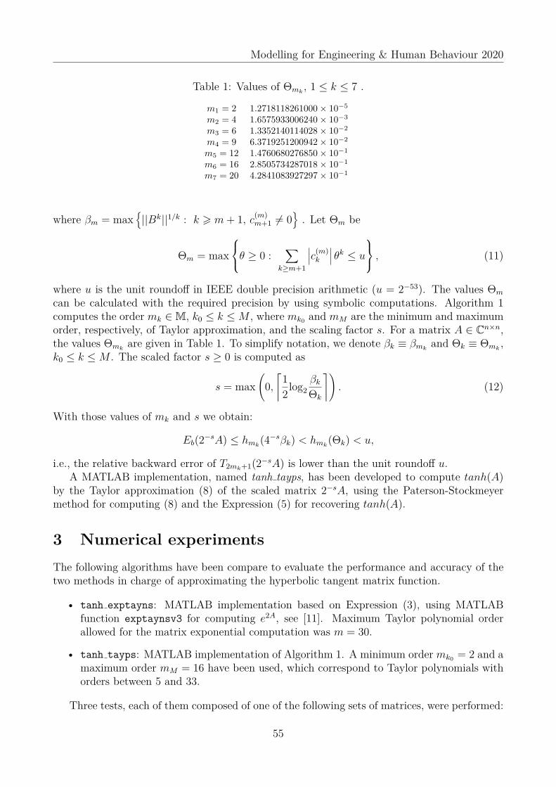
Table 1: Values of Θmk , 1 ≤ k ≤ 7 .

m1 = 2 1.2718118261000× 10−5

m2 = 4 1.6575933006240× 10−3

m3 = 6 1.3352140114028× 10−2

m4 = 9 6.3719251200942× 10−2

m5 = 12 1.4760680276850× 10−1

m6 = 16 2.8505734287018× 10−1

m7 = 20 4.2841083927297× 10−1

where βm = max{||Bk||1/k : k > m+ 1, c(m)

m+1 6= 0}

. Let Θm be

Θm = maxθ ≥ 0 :

∑k≥m+1

∣∣∣c(m)k

∣∣∣ θk ≤ u

, (11)

where u is the unit roundoff in IEEE double precision arithmetic (u = 2−53). The values Θm

can be calculated with the required precision by using symbolic computations. Algorithm 1computes the order mk ∈M, k0 ≤ k ≤M , where mk0 and mM are the minimum and maximumorder, respectively, of Taylor approximation, and the scaling factor s. For a matrix A ∈ Cn×n,the values Θmk are given in Table 1. To simplify notation, we denote βk ≡ βmk and Θk ≡ Θmk ,k0 ≤ k ≤M . The scaled factor s ≥ 0 is computed as

s = max(

0,⌈

12log2

βkΘk

⌉). (12)

With those values of mk and s we obtain:

Eb(2−sA) ≤ hmk(4−sβk) < hmk(Θk) < u,

i.e., the relative backward error of T2mk+1(2−sA) is lower than the unit roundoff u.A MATLAB implementation, named tanh tayps, has been developed to compute tanh(A)

by the Taylor approximation (8) of the scaled matrix 2−sA, using the Paterson-Stockmeyermethod for computing (8) and the Expression (5) for recovering tanh(A).

3 Numerical experimentsThe following algorithms have been compare to evaluate the performance and accuracy of thetwo methods in charge of approximating the hyperbolic tangent matrix function.

• tanh exptayns: MATLAB implementation based on Expression (3), using MATLABfunction exptaynsv3 for computing e2A, see [11]. Maximum Taylor polynomial orderallowed for the matrix exponential computation was m = 30.

• tanh tayps: MATLAB implementation of Algorithm 1. A minimum order mk0 = 2 and amaximum order mM = 16 have been used, which correspond to Taylor polynomials withorders between 5 and 33.

Three tests, each of them composed of one of the following sets of matrices, were performed:

55

Modelling for Engineering & Human Behaviour 2020

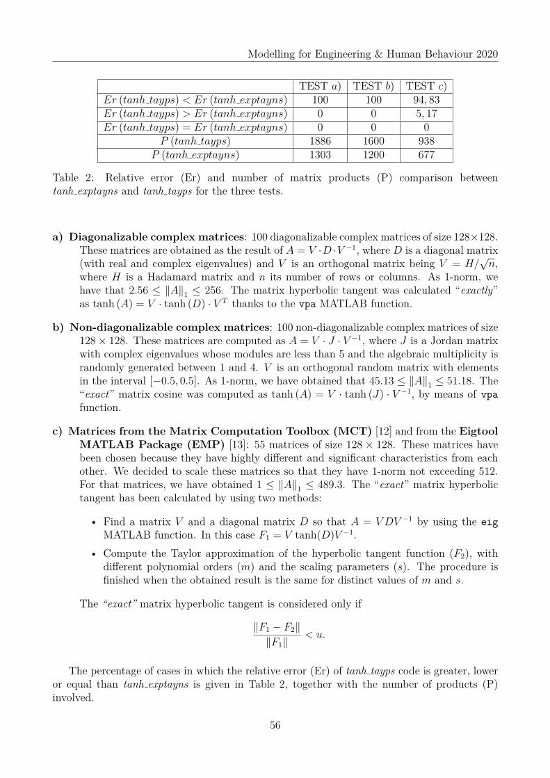
TEST a) TEST b) TEST c)Er (tanh tayps) < Er (tanh exptayns) 100 100 94, 83Er (tanh tayps) > Er (tanh exptayns) 0 0 5, 17Er (tanh tayps) = Er (tanh exptayns) 0 0 0

P (tanh tayps) 1886 1600 938P (tanh exptayns) 1303 1200 677

Table 2: Relative error (Er) and number of matrix products (P) comparison betweentanh exptayns and tanh tayps for the three tests.

a) Diagonalizable complex matrices: 100 diagonalizable complex matrices of size 128×128.These matrices are obtained as the result of A = V ·D ·V −1, where D is a diagonal matrix(with real and complex eigenvalues) and V is an orthogonal matrix being V = H/

√n,

where H is a Hadamard matrix and n its number of rows or columns. As 1-norm, wehave that 2.56 ≤ ‖A‖1 ≤ 256. The matrix hyperbolic tangent was calculated “exactly”as tanh (A) = V · tanh (D) · V T thanks to the vpa MATLAB function.

b) Non-diagonalizable complex matrices: 100 non-diagonalizable complex matrices of size128× 128. These matrices are computed as A = V · J · V −1, where J is a Jordan matrixwith complex eigenvalues whose modules are less than 5 and the algebraic multiplicity israndomly generated between 1 and 4. V is an orthogonal random matrix with elementsin the interval [−0.5, 0.5]. As 1-norm, we have obtained that 45.13 ≤ ‖A‖1 ≤ 51.18. The“exact” matrix cosine was computed as tanh (A) = V · tanh (J) · V −1, by means of vpafunction.

c) Matrices from the Matrix Computation Toolbox (MCT) [12] and from the EigtoolMATLAB Package (EMP) [13]: 55 matrices of size 128 × 128. These matrices havebeen chosen because they have highly different and significant characteristics from eachother. We decided to scale these matrices so that they have 1-norm not exceeding 512.For that matrices, we have obtained 1 ≤ ‖A‖1 ≤ 489.3. The “exact” matrix hyperbolictangent has been calculated by using two methods:

• Find a matrix V and a diagonal matrix D so that A = V DV −1 by using the eigMATLAB function. In this case F1 = V tanh(D)V −1.

• Compute the Taylor approximation of the hyperbolic tangent function (F2), withdifferent polynomial orders (m) and the scaling parameters (s). The procedure isfinished when the obtained result is the same for distinct values of m and s.

The “exact” matrix hyperbolic tangent is considered only if

‖F1 − F2‖‖F1‖

< u.

The percentage of cases in which the relative error (Er) of tanh tayps code is greater, loweror equal than tanh exptayns is given in Table 2, together with the number of products (P)involved.

56

Modelling for Engineering & Human Behaviour 2020

4 ConclusionsAs deduced from the results given in Table 2, in the vast majority of cases, algorithm tanh taypsis more accurate than tanh exptayns although with a little more computational cost. This sup-ports the recommendation made in [14] to use Taylor’s development against other alternatives,whenever possible.

AcknowledgementsThis work has been partially supported by Spanish Ministerio de Economıa y Competitividadand European Regional Development Fund (ERDF) grants TIN2017-89314-P and by the Pro-grama de Apoyo a la Investigacion y Desarrollo 2018 of the Universitat Politecnica de Valencia(PAID-06-18) grants SP20180016.

References[1] Garij V. Efimov, Wilhelm Von Waldenfels, Rainer Wehrse, Analytical solution of the

non-discretized radiative transfer equation for a slab of finite optical depth Journal ofQuantitative Spectroscopy and Radiative Transfer, 53(1): 59–74, 1995.

[2] Antti Lehtinen, Analytical treatment of heat sinks cooled by forced convection (PhD the-sis). Tampere University of Technology, Finland, 2005.

[3] Kaj Lampio, Optimization of fin arrays cooled by forced or natural convection (PhD thesis).Tampere University of Technology, Finland, 2018.

[4] R. Hilscher, P. Zemanek,Trigonometric and hyperbolic systems on time scales DynamicSystems and Applications, 18(3): 162–184, 2009.

[5] P. Zemanek, New Results in Theory of Symplectic Systems on Time Scales (PhD thesis).Masarykova Univerzita, Czech Republic, 2011.

[6] Ernesto Estrada, Grant Silver, Accounting for the role of long walks on networks via a newmatrix function Journal of Mathematical Analysis and Applications, 449(2): 1581–1600,2017.

[7] J. Sastre, J. Ibanez, E. Defez, P. Ruiz, New scaling-squaring Taylor algorithms for com-puting the matrix exponential SIAM Journal on Scientific Computing, 37(1): A439–A455,2015.

[8] J. Sastre, J. Ibanez, E. Defez, P. Ruiz, Efficient orthogonal matrix polynomial basedmethod for computing matrix exponential Applied Mathematics and Computation, 217(14):6451–6463, 2011.

[9] E. Defez, J. Ibanez, P. Alonso-Jorda, Jose M. Alonso, J. Peinado, On Bernoulli matrixpolynomials and matrix exponential approximation Journal of Computational and AppliedMathematics, https://doi.org/10.1016/j.cam.2020.113207.

57

Modelling for Engineering & Human Behaviour 2020

[10] Michael S. Paterson, Larry J. Stockmeyer, On the number of nonscalar multiplicationsnecessary to evaluate polynomials SIAM Journal on Computing, 2(1): 60–66, 1973.

[11] P. Ruiz, J. Sastre, J. Ibanez, E. Defez, High perfomance computing of the matrix expo-nential Journal of Computational and Applied Mathematics, 291: 370–379, 2016.

[12] N. J. Higham, The matrix computation toolbox, http://www.ma.man.ac.uk/higham/mctoolbox. 2002.

[13] T.G. Wright, Eigtool, version 2.1. http://www.comlab.ox.ac.uk/pseudospectra/eigtool. 2009

[14] James Corwell, William Dale Blair, Industry Tip: Quick and Easy Matrix ExponentialsIEEE Aerospace and Electronic Systems Magazine, 35(5): 49–52, 2020.

58