Modelling Chemical Reactions

Sample Modelling Activities with Excel and Modellus

ITforUS

(Information Technology for Understanding Science)

© 2007 IT for US - The project is funded with support from the European Commission 119001-CP-1-2004-1-PL-COMENIUS-C21. This publication reflects the views only of the author, and the Commission cannot be held responsible for any use of the information contained therein.

2

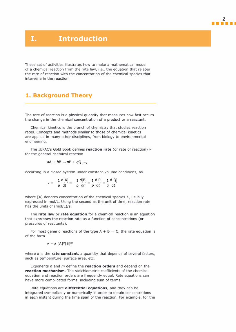
These set of activities illustrates how to make a mathematical model of a chemical reaction from the rate law, i.e., the equation that relates the rate of reaction with the concentration of the chemical species that intervene in the reaction.

1. Background Theory

The rate of reaction is a physical quantity that measures how fast occurs the change in the chemical concentration of a product or a reactant.

Chemical kinetics is the branch of chemistry that studies reaction rates. Concepts and methods similar to those of chemical kinetics are applied in many other disciplines, from biology to environmental engineering.

The IUPAC’s Gold Book defines reaction rate (or rate of reaction) v for the general chemical reaction

aA + bB ® pP + qQ ...,

occurring in a closed system under constant-volume conditions, as

v

a t b t p t q t= -

[ ]= -

[ ]=

[ ]=

[ ]1 1 1 1d A

d

d B

d

d P

d

d Q

d

where [X] denotes concentration of the chemical species X, usually expressed in mol/L. Using the second as the unit of time, reaction rate has the units of (mol/L)/s.

The rate law or rate equation for a chemical reaction is an equation that expresses the reaction rate as a function of concentrations (or pressures of reactants).

For most generic reactions of the type A + B ® C, the rate equation is of the form

v = k [A]n[B]m

where k is the rate constant, a quantity that depends of several factors, such as temperature, surface area, etc.

Exponents n and m define the reaction orders and depend on the reaction mechanism. The stoichiometric coefficients of the chemical equation and reaction orders are frequently equal. Rate equations can have more complicated forms, including sum of terms.

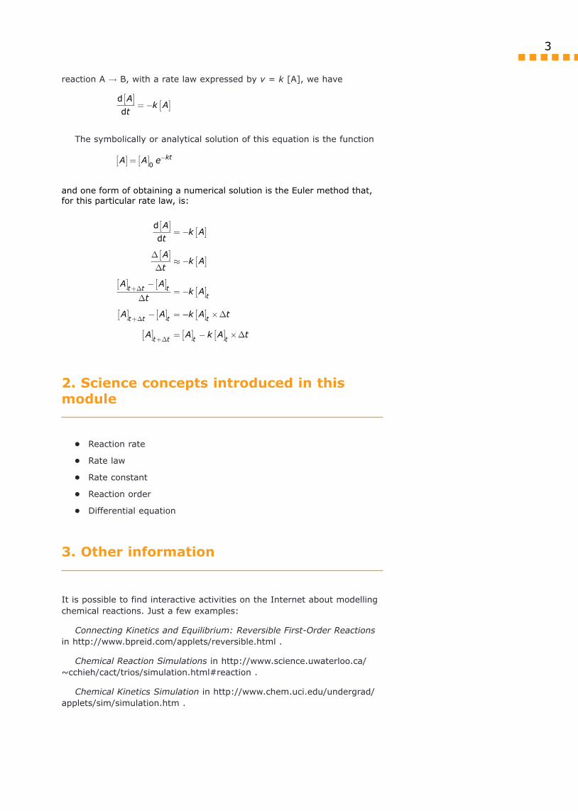
Rate equations are differential equations, and they can be integrated symbolically or numerically in order to obtain concentrations in each instant during the time span of the reaction. For example, for the

I. Introduction

3

2. Science concepts introduced in this module

• Reaction rate

• Rate law

• Rate constant

• Reaction order

• Differential equation

3. Other information

It is possible to find interactive activities on the Internet about modelling chemical reactions. Just a few examples:

Connecting Kinetics and Equilibrium: Reversible First-Order Reactions in http://www.bpreid.com/applets/reversible.html .

Chemical Reaction Simulations in http://www.science.uwaterloo.ca/~cchieh/cact/trios/simulation.html#reaction .

Chemical Kinetics Simulation in http://www.chem.uci.edu/undergrad/applets/sim/simulation.htm .

reaction A ® B, with a rate law expressed by v = k [A], we have

d

d

A

tk A

[ ]= - [ ]

The symbolically or analytical solution of this equation is the function

A A e kt[ ] = [ ] -

0

and one form of obtaining a numerical solution is the Euler method that, for this particular rate law, is:

d

d

A

tk A

A

tk A

A A

tk A

A A

t t tt

t t t

[ ]= - [ ]

[ ]» - [ ]

[ ] - [ ]= - [ ]

[ ] - [ ] =

+

+

D

D

DD

D-- [ ] ´

[ ] = [ ] - [ ] ´+

k A t

A A k A t

t

t t t t

D

DD

4

1. Pedagogical context

The activities presented in this module can be used with students of upper secondary school, first year college students and secondary teachers, either in Chemistry or in Mathematics classes.

They were not designed to fit in any curriculum. They simple illustrate how two interactive computer tools (Modellus and a spreadsheet like Excel) can be used to model physical phenomena. They can be particularly useful for simultaneous training of Chemistry and Mathematics teachers, promoting interdisciplinarity and reflection about concepts and representations and for the introduction of simple numerical methods.

2. Common student difficulties

Some of the student difficulties include:

• Interpreting graphs with time as the independent variable plot-ted on the horizontal axis.

• Using rates of change to define equivalent iterative equations.

• Assuming that all rate laws are expressed using stoichiometric co-effiecients.

• Assuming that equilibrium means “the end of the reaction”.

3. Evaluation of ICT

Computers are now the most common scientific tool, used in almost all aspects of the scientific endeavour, from measuring and modelling to writing and synchronous communication. It should then be natural to use computers in learning science.

The spreadsheet is an excellent tool when large number of repetitive calculations need to be made, such as variables that are incrementally changed, and data must be presented graphically. In chemical kinetics and equilibrium, the numerical solution of the rate laws can easily be implemented using iterative equations of the type

new value = old value + rate of change ´ small time interval

II. Didactical approach

5

4. Teaching approaches

Good classroom organization is an essential component in a successful teaching approach, particularly when using complex tools such as computers and software. Most approaches to classroom organization that can give good results mix features of students’ autonomous work, both individually and in small groups, to teacher lecturing to all class.

Typically, teachers can start with an all class approach, with students following the lesson with a screen projector. It is almost always a good idea to ask one or more students to work on the computer connected to the projector. This allows the teacher to have direct information of students’ difficulties when manipulating the software and to be slower on the explanation of the ideas and activities that are being presented.

As all teachers know by experience, it is usually difficult for most students to follow written instructions, even when these instructions are only a few sentences long. To overcome this difficulty, teachers can ask students to read the activities before starting them and then promote a collective or group discussion about what is supposed to be done with the computer. As a rule of thumb, students should only start an activity when they know what they will do on the activity: they will only consult the written worksheet just for checking details, not for following instructions.

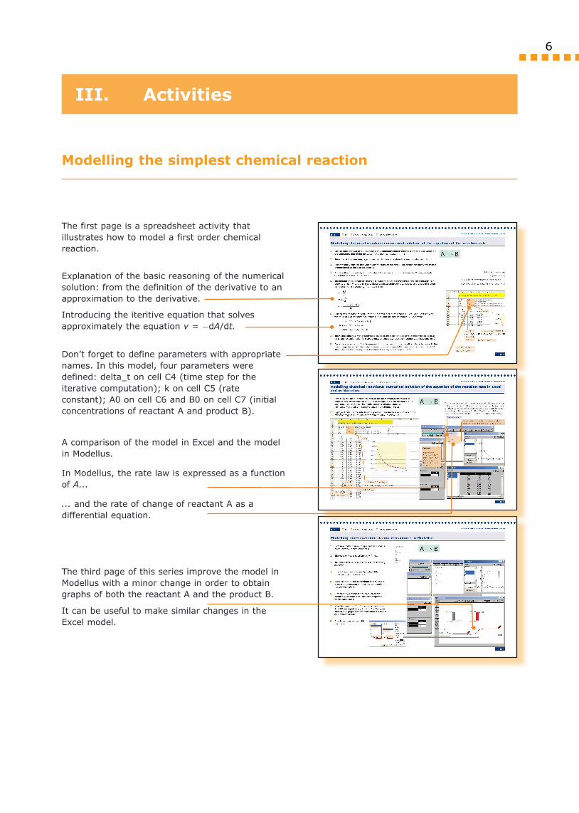
Modelling the simplest chemical reaction

The first page is a spreadsheet activity that illustrates how to model a first order chemical reaction.

Explanation of the basic reasoning of the numerical solution: from the definition of the derivative to an approximation to the derivative.

Introducing the iteritive equation that solves approximately the equation v = -dA/dt.

Don’t forget to define parameters with appropriate names. In this model, four parameters were defined: delta_t on cell C4 (time step for the iterative computation); k on cell C5 (rate constant); A0 on cell C6 and B0 on cell C7 (initial concentrations of reactant A and product B).

A comparison of the model in Excel and the model in Modellus.

In Modellus, the rate law is expressed as a function of A...

... and the rate of change of reactant A as a differential equation.

The third page of this series improve the model in Modellus with a minor change in order to obtain graphs of both the reactant A and the product B.

It can be useful to make similar changes in the Excel model.

6

III. Activities

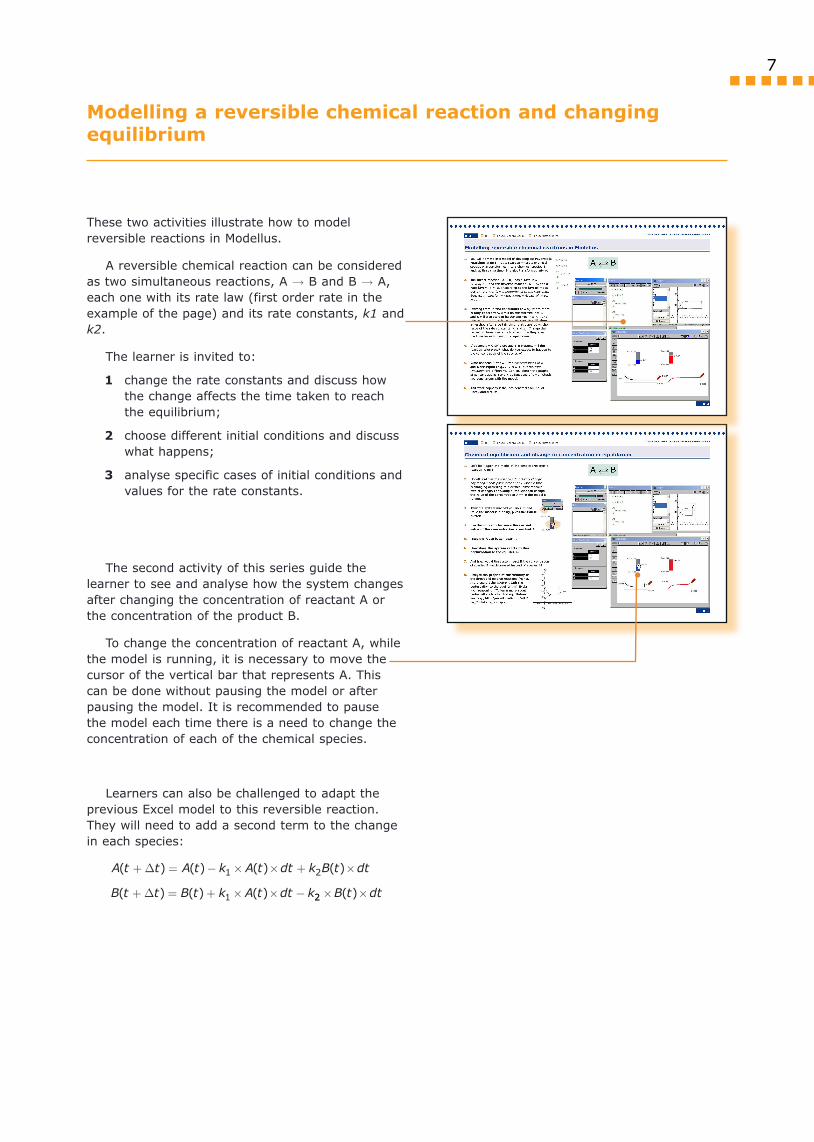
Modelling a reversible chemical reaction and changing equilibrium

These two activities illustrate how to model reversible reactions in Modellus.

A reversible chemical reaction can be considered as two simultaneous reactions, A ® B and B ® A, each one with its rate law (first order rate in the example of the page) and its rate constants, k1 and k2.

The learner is invited to:

1 change the rate constants and discuss how the change affects the time taken to reach the equilibrium;

2 choose different initial conditions and discuss what happens;

3 analyse specific cases of initial conditions and values for the rate constants.

The second activity of this series guide the learner to see and analyse how the system changes after changing the concentration of reactant A or the concentration of the product B.

To change the concentration of reactant A, while the model is running, it is necessary to move the cursor of the vertical bar that represents A. This can be done without pausing the model or after pausing the model. It is recommended to pause the model each time there is a need to change the concentration of each of the chemical species.

Learners can also be challenged to adapt the previous Excel model to this reversible reaction. They will need to add a second term to the change in each species:

A t t A t k A t dt k B t dt

B t t B t k A t dt k

( ) ( ) ( ) ( )

( ) ( ) ( )

+ = - ´ ´ + ´

+ = + ´ ´ -

D

D

1 2

1 22 ´ ´B t dt( )

7

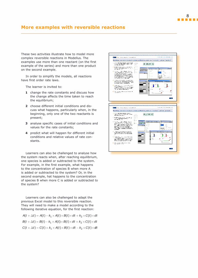
More examples with reversible reactions

These two activities illustrate how to model more complex reversible reactions in Modellus. The examples use more than one reactant (on the first example of the series) and more than one product on the second example.

In order to simplify the models, all reactions have first order rate laws.

The learner is invited to:

1 change the rate constants and discuss how the change affects the time taken to reach the equilibrium;

2 choose different initial conditions and dis-cuss what happens, particularly when, in the beginning, only one of the two reactants is present;

3 analyse specific cases of initial conditions and values for the rate constants;

4 predict what will happen for different initial conditions and relative values of rate con-stants.

Learners can also be challenged to analyse how the system reacts when, after reaching equilibrium, one species is added or subtracted to the system. For example, in the first example, what happens to the concentration of species B when more A is added or subtracted to the system? Or, in the second example, hat happens to the concentration of species B when more C is added or subtracted to the system?

Learners can also be challenged to adapt the previous Excel model to this reversible reaction. They will need to make a model according to the following iterative equation, for the first reaction:

A t t A t k A t B t dt k C t dt

B t t B t k A t

( ) ( ) ( ) ( ) ( )

( ) ( ) (

+ = - ´ ´ ´ + ´ ´

+ = - ´

D

D

1 2

1 )) ( ) ( )

( ) ( ) ( ) ( ) ( )

´ ´ + ´ ´

+ = + ´ ´ ´ - ´ ´

B t dt k C t dt

C t t C t k A t B t dt k C t

2

1 2D ddt

8

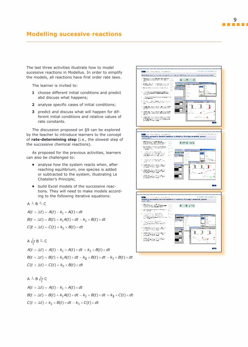
Modelling sucessive reactions

The last three activities illustrate how to model sucessive reactions in Modellus. In order to simplify the models, all reactions have first order rate laws.

The learner is invited to:

1 choose different initial conditions and predict abd discuss what happens;

2 analyse specific cases of initial conditions;

3 predict and discuss what will happen for dif-ferent initial conditions and relative values of rate constants.

The discussion proposed on §9 can be explored by the teacher to introduce learners to the concept of rate-determining step (i.e., the slowest step of the successive chemical reactions).

As proposed for the previous activities, learners can also be challenged to:

• analyse how the system reacts when, after reaching equilibrium, one species is added or subtracted to the system, illustrating Le Chatelier’s Principle;

• build Excel models of the successive reac-tions. They will need to make models accord-ing to the following iterative equations:

A t t A t k A t dt

B t t B t k A t dt k B t dt

C

( ) ( ) ( )

( ) ( ) ( ) ( )

(

+ = - ´ ´

+ = + ´ - ´ ´

D

D

1

1 2

tt t C t k B t dt+ = + ´ ´D ) ( ) ( )2

A t t A t k A t dt k B t dt

B t t B t k A t dt k

( ) ( ) ( ) ( )

( ) ( ) ( )

+ = - ´ ´ + ´ ´

+ = + ´ -

D

D

1 2

1 22 3

3

´ ´ - ´ ´

+ = + ´ ´

B t dt k B t dt

C t t C t k B t dt

( ) ( )

( ) ( ) ( )D

A t t A t k A t dt

B t t B t k A t dt k B t dt k

( ) ( ) ( )

( ) ( ) ( ) ( )

+ = - ´ ´

+ = + ´ - ´ ´ +

D

D

1

1 2 33

2 3

´ ´

+ = ´ ´ - ´ ´

C t dt

C t t k B t dt k C t dt

( )

( ) ( ) ( )D

A B C® ®1 2

A B C ®1

23

A B C®

1

3

2

9