Lesson Overview Lesson Overview Aquatic Ecosystems Lesson Overview 4.5 Aquatic Ecosystems.
Modelling Aquatic EcosystemsCourse 701-0426-00, ETH Zürich
Spring 2017Nele Schuwirth & Peter [email protected], [email protected]
ETH Zürich, Department of Environmental Systems SciencesEawag, Swiss Federal Institute of Aquatic Science and Technology
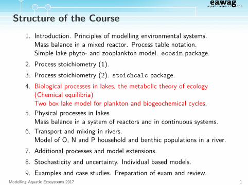
Structure of the Course1. Introduction. Principles of modelling environmental systems.
Mass balance in a mixed reactor. Process table notation.Simple lake phyto- and zooplankton model. ecosim package.
2. Process stoichiometry (1).3. Process stoichiometry (2). stoichcalc package.4. Biological processes in lakes, the metabolic theory of ecology
(Chemical equilibria)Two box lake model for plankton and biogeochemical cycles.
5. Physical processes in lakesMass balance in a system of reactors and in continuous systems.
6. Transport and mixing in rivers.Model of O, N and P household and benthic populations in a river.
7. Additional processes and model extensions.8. Stochasticity and uncertainty. Individual based models.9. Examples and case studies. Preparation of exam and review.
Modelling Aquatic Ecosystems 2017 1
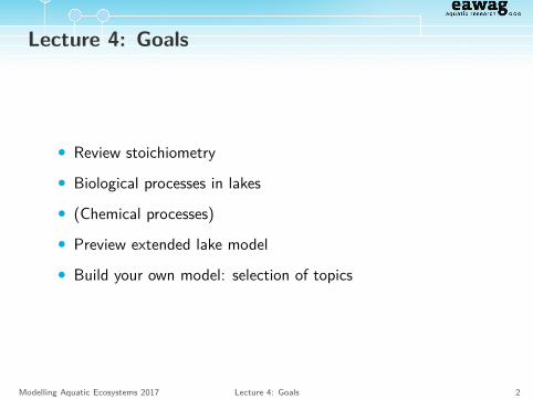
Lecture 4: Goals
• Review stoichiometry
• Biological processes in lakes
• (Chemical processes)
• Preview extended lake model
• Build your own model: selection of topics
Modelling Aquatic Ecosystems 2017 Lecture 4: Goals 2
New Challenge: Develop your own model
During the semester you have to develop and implement your ownmodel (alone or in groups of two), interpret simulation results andperform a simple sensitivity analysis.
We provide two topics to choose from.We will assign topics on 29.03.2017 (today).
You will deliver the R-files and results by the end of the semester(2.6.2017!) per email to [email protected].
In the oral exam we will ask you about your example (beside othertopics).
Modelling Aquatic Ecosystems 2017 Lecture 4: Goals 3
Process Stoichiometry
How to derive the stoichiometric coefficients νij?
• Chemical substance notation.
• Parameterized elemental mass fractions.
• General solution.
Modelling Aquatic Ecosystems 2017 Lecture 4: Review Stoichiometry 4

Review Stoichiometry
Questions to think about:
• Is it important to know the number of independent processespossible for a given set of substances of known composition?
• How can the number of required additional constraints bederived easily?Under which circumstances would this simple approach fail?
• Where to get the required additional constraints from?
Modelling Aquatic Ecosystems 2017 Lecture 4: Review Stoichiometry 5
Biological processes
It’s your turn:
• What happens in the process?Which substances/organisms are involved?• Explain qualitatative stoichiometry (process table).Additional constraints?• Explain the process rate.• Anything else special?
10 Minutes for preparation!
Modelling Aquatic Ecosystems 2017 Lecture 4: Biological Processes 6
Primary Production
What happens?
Primary production is the production of organic material frominorganic nutrients through photosynthesis.
This process provides the food for the subsequent trophic levels ofthe ecosystem foodweb.
Modelling Aquatic Ecosystems 2017 Lecture 4: Biological Processes 7
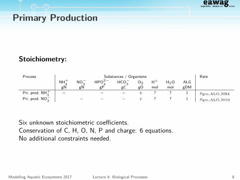
Primary Production
Stoichiometry:
Process Substances / Organisms RateNH+
4 NO−3 HPO2−
4 HCO−3 O2 H+ H2O ALG
gN gN gP gC gO mol mol gDMPri. prod. NH+
4 − − − + ? ? 1 ρgro,ALG,NH4Pri. prod. NO−
3 − − − + ? ? 1 ρgro,ALG,NO3
Six unknown stoichiometric coefficients.Conservation of C, H, O, N, P and charge: 6 equations.No additional constraints needed.
Modelling Aquatic Ecosystems 2017 Lecture 4: Biological Processes 8
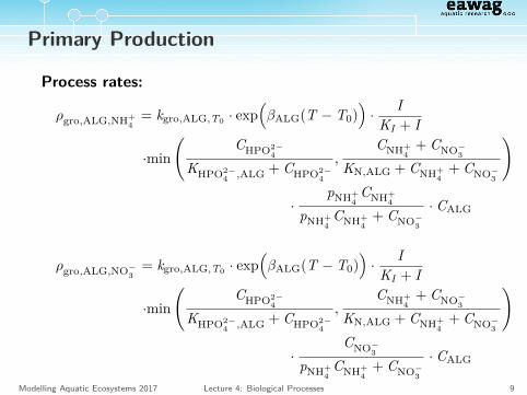
Primary Production
Process rates:
ρgro,ALG,NH+4
= kgro,ALG,T0 · exp(βALG(T − T0)
)· I
KI + I
·min(
CHPO2−4
KHPO2−4 ,ALG + CHPO2−
4
,CNH+
4+ CNO−
3
KN,ALG + CNH+4
+ CNO−3
)
·pNH+
4CNH+
4
pNH+4
CNH+4
+ CNO−3
· CALG
ρgro,ALG,NO−3
= kgro,ALG,T0 · exp(βALG(T − T0)
)· I
KI + I
·min(
CHPO2−4
KHPO2−4 ,ALG + CHPO2−
4
,CNH+
4+ CNO−
3
KN,ALG + CNH+4
+ CNO−3
)
·CNO−
3
pNH+4
CNH+4
+ CNO−3
· CALG
Modelling Aquatic Ecosystems 2017 Lecture 4: Biological Processes 9
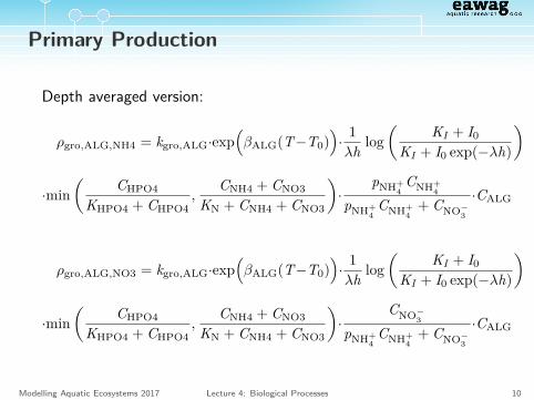
Primary Production
Depth averaged version:
ρgro,ALG,NH4 = kgro,ALG·exp(βALG(T−T0)
)· 1λh log
(KI + I0
KI + I0 exp(−λh)
)
·min(
CHPO4
KHPO4 + CHPO4,
CNH4 + CNO3
KN + CNH4 + CNO3
)·
pNH+4
CNH+4
pNH+4
CNH+4
+ CNO−3
·CALG
ρgro,ALG,NO3 = kgro,ALG·exp(βALG(T−T0)
)· 1λh log
(KI + I0
KI + I0 exp(−λh)
)
·min(
CHPO4
KHPO4 + CHPO4,
CNH4 + CNO3
KN + CNH4 + CNO3
)·
CNO−3
pNH+4
CNH+4
+ CNO−3
·CALG
Modelling Aquatic Ecosystems 2017 Lecture 4: Biological Processes 10
Respiration
Respiration is the inverse process of photosynthesis.
Respiration is an important process for the survival of organisms asit frees energy for live maintenance processes.
Respiration leads to cycling of nutrients between the organicallybound and inorganic phases.
Modelling Aquatic Ecosystems 2017 Lecture 4: Biological Processes 11
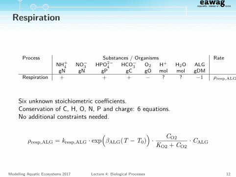
Respiration
Process Substances / Organisms RateNH+
4 NO−3 HPO2−4 HCO−3 O2 H+ H2O ALG
gN gN gP gC gO mol mol gDMRespiration + + + − ? ? −1 ρresp,ALG
Six unknown stoichiometric coefficients.Conservation of C, H, O, N, P and charge: 6 equations.No additional constraints needed.
ρresp,ALG = kresp,ALG · exp(βALG(T − T0)
)· CO2
KO2 + CO2· CALG
Modelling Aquatic Ecosystems 2017 Lecture 4: Biological Processes 12
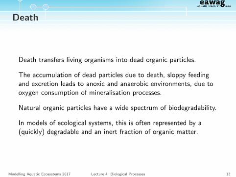
Death
Death transfers living organisms into dead organic particles.
The accumulation of dead particles due to death, sloppy feedingand excretion leads to anoxic and anaerobic environments, due tooxygen consumption of mineralisation processes.
Natural organic particles have a wide spectrum of biodegradability.
In models of ecological systems, this is often represented by a(quickly) degradable and an inert fraction of organic matter.
Modelling Aquatic Ecosystems 2017 Lecture 4: Biological Processes 13
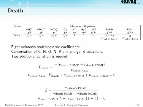
Death
Process Substances / Organisms RateNH+
4 HPO2−4 HCO−
3 O2 H+ H2O ALG POMD POMIgN gP gC gO mol mol gDM gDM gDM
Death 0/+ 0/+ 0/+ 0/+ ? ? −1 (1− fI) fI ρdeath,ALG·YALG,death ·YALG,death
Eight unknown stoichiometric coefficients.Conservation of C, H, O, N, P and charge: 6 equations.Two additional constraints needed:
Ydeath = −(νdeath POMD + νdeath POMI)νdeath ALG
νdeath ALG ·Ydeath + νdeath POMD + νdeath POMI = 0
fI = −νdeath POMI
νdeath POMI + νdeath POMD
νdeath POMD fI − νdeath POMI(1− fI) = 0Modelling Aquatic Ecosystems 2017 Lecture 4: Biological Processes 14
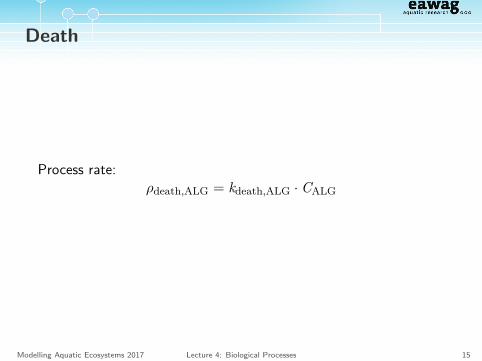
Death
Process rate:ρdeath,ALG = kdeath,ALG · CALG
Modelling Aquatic Ecosystems 2017 Lecture 4: Biological Processes 15
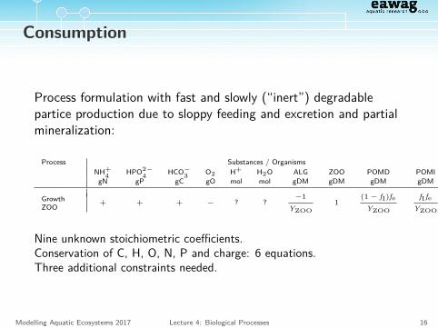
Consumption
Process formulation with fast and slowly (“inert”) degradablepartice production due to sloppy feeding and excretion and partialmineralization:
Process Substances / Organisms RateNH+
4 HPO2−4 HCO−
3 O2 H+ H2O ALG ZOO POMD POMIgN gP gC gO mol mol gDM gDM gDM gDM
GrowthZOO + + + − ? ?
−1YZOO
1(1− fI)fe
YZOO
fIfe
YZOOρgro,ZOO
Nine unknown stoichiometric coefficients.Conservation of C, H, O, N, P and charge: 6 equations.Three additional constraints needed.
Modelling Aquatic Ecosystems 2017 Lecture 4: Biological Processes 16
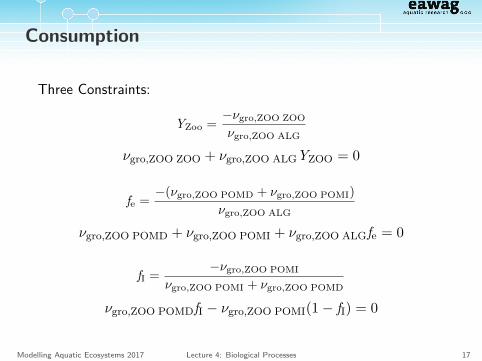
Consumption
Three Constraints:
YZoo = −νgro,ZOO ZOO
νgro,ZOO ALG
νgro,ZOO ZOO + νgro,ZOO ALGYZOO = 0
fe = −(νgro,ZOO POMD + νgro,ZOO POMI)νgro,ZOO ALG
νgro,ZOO POMD + νgro,ZOO POMI + νgro,ZOO ALGfe = 0
fI = −νgro,ZOO POMI
νgro,ZOO POMI + νgro,ZOO POMD
νgro,ZOO POMDfI − νgro,ZOO POMI(1− fI) = 0
Modelling Aquatic Ecosystems 2017 Lecture 4: Biological Processes 17
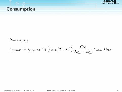
Consumption
Process rate:
ρgro,ZOO = kgro,ZOO·exp(βALG(T−T0)
)· CO2KO2 + CO2
·CALG·CZOO
Modelling Aquatic Ecosystems 2017 Lecture 4: Biological Processes 18
Mineralization
Oxic mineralization transforms organic matter to dissolvednutrients and carbon dioxide under consumption of oxygen.
In the absence of dissolved oxygen (primarily in the sediment),mineralization can use nitrate, manganese oxide, iron hydroxide orsulfate for oxidizing organic matter.
Finally, methanogenesis can convert organic matter to nutrients,carbon dioxide and methane.
As mineralization is caused by bacteria and bacterial concentra-tions vary considerably from one (part of the) system to another,mineralization rate coefficients vary over many orders ofmagnitude.
Modelling Aquatic Ecosystems 2017 Lecture 4: Biological Processes 19
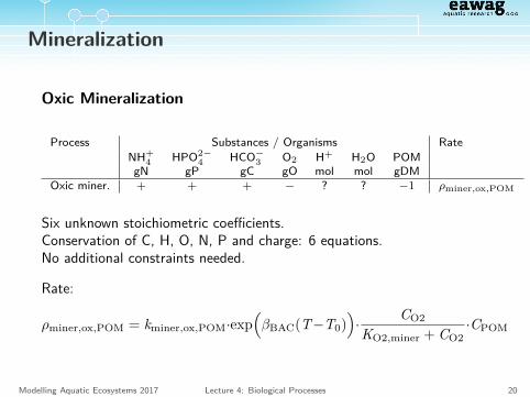
Mineralization
Oxic Mineralization
Process Substances / Organisms RateNH+
4 HPO2−4 HCO−3 O2 H+ H2O POM
gN gP gC gO mol mol gDMOxic miner. + + + − ? ? −1 ρminer,ox,POM
Six unknown stoichiometric coefficients.Conservation of C, H, O, N, P and charge: 6 equations.No additional constraints needed.
Rate:
ρminer,ox,POM = kminer,ox,POM·exp(βBAC(T−T0)
)· CO2
KO2,miner + CO2·CPOM
Modelling Aquatic Ecosystems 2017 Lecture 4: Biological Processes 20
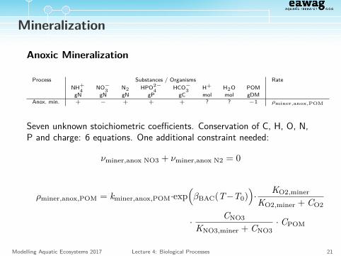
Mineralization
Anoxic Mineralization
Process Substances / Organisms RateNH+
4 NO−3 N2 HPO2−
4 HCO−3 H+ H2O POM
gN gN gN gP gC mol mol gDMAnox. min. + − + + + ? ? −1 ρminer,anox,POM
Seven unknown stoichiometric coefficients. Conservation of C, H, O, N,P and charge: 6 equations. One additional constraint needed:
νminer,anox NO3 + νminer,anox N2 = 0
ρminer,anox,POM = kminer,anox,POM·exp(βBAC(T−T0)
)· KO2,miner
KO2,miner + CO2
· CNO3
KNO3,miner + CNO3· CPOM
Modelling Aquatic Ecosystems 2017 Lecture 4: Biological Processes 21
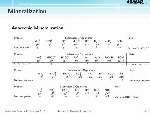
Mineralization
Anaerobic Mineralization
Process Substances / Organisms RateNH+
4 HPO2−4 HCO−
3 Mn2+ H+ H2O MnO2 POMgN gP gC mol mol mol mol gDM
Mn oxide red. + + + + ? ? − −1 ρminer,MnO2,POM
Process Substances / Organisms RateNH+
4 HPO2−4 HCO−
3 Fe2+ H+ H2O FeOOH POMgN gP gC mol mol mol mol gDM
Fe hydrox. red. + + + + ? ? − −1 ρminer,FeOOH,POM
Process Substances / Organisms RateNH+
4 HPO2−4 HCO−
3 SO2−4 HS− H+ H2O POM
gN gP gC mol mol mol mol gDMSulfate reduction + + + − + ? ? −1 ρminer,SO4,POM
Process Substances / Organisms RateNH+
4 HPO2−4 HCO−
3 CH4 H+ H2O POMgN gP gC gC mol mol gDM
Methanogenesis + + + + ? ? −1 ρminer,CH4,POM
Modelling Aquatic Ecosystems 2017 Lecture 4: Biological Processes 22
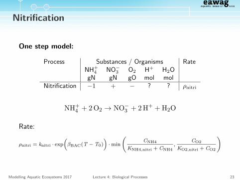
Nitrification
One step model:
Process Substances / Organisms RateNH+
4 NO−3 O2 H+ H2O
gN gN gO mol molNitrification −1 + − ? ? ρnitri
NH+4 + 2 O2 → NO−
3 + 2 H+ + H2O
Rate:
ρnitri = knitri · exp(βBAC(T − T0)
)· min
(CNH4
KNH4,nitri + CNH4,
CO2KO2,nitri + CO2
)
Modelling Aquatic Ecosystems 2017 Lecture 4: Biological Processes 23
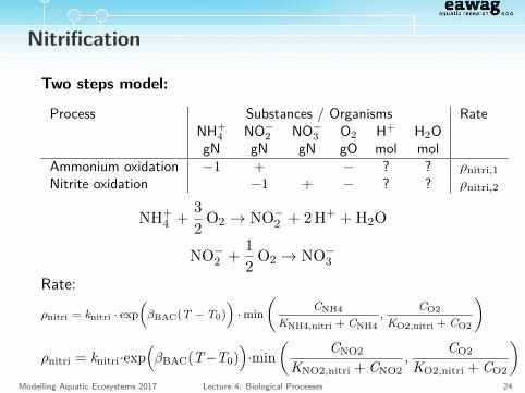
Nitrification
Two steps model:
Process Substances / Organisms RateNH+
4 NO−2 NO−
3 O2 H+ H2OgN gN gN gO mol mol
Ammonium oxidation −1 + − ? ? ρnitri,1Nitrite oxidation −1 + − ? ? ρnitri,2
NH+4 + 3
2 O2 → NO−2 + 2 H+ + H2O
NO−2 + 1
2 O2 → NO−3
Rate:
ρnitri = knitri · exp(βBAC(T − T0)
)· min
(CNH4
KNH4,nitri + CNH4,
CO2KO2,nitri + CO2
)ρnitri = knitri·exp
(βBAC(T−T0)
)·min
(CNO2
KNO2,nitri + CNO2,
CO2
KO2,nitri + CO2
)Modelling Aquatic Ecosystems 2017 Lecture 4: Biological Processes 24
Modelling Individual Taxa
There is no fundamental difference between modelling functionalgroups or individual taxa.
However, the number of taxa is much larger than the number offunctional groups. This leads to an extreme increase in the numberof model parameters.
This can be handled by applying the Metabolic Theory of Ecology.
Modelling Aquatic Ecosystems 2017 Lecture 4: The Metabolic Theory of Ecology 25
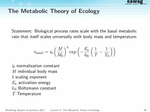
The Metabolic Theory of Ecology
Statement: Biological process rates scale with the basal metabolicrate that itself scales universally with body mass and temperature:
rbasal = i0( M
M0
)bexp
(−Ea
kB
( 1T −
1T0
))
i0 normalization constantM individual body massb scaling exponentEa activation energykB Boltzmann constantT Temperature
Modelling Aquatic Ecosystems 2017 Lecture 4: The Metabolic Theory of Ecology 26
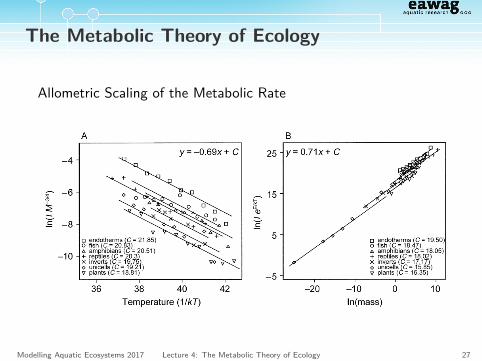
The Metabolic Theory of Ecology
Allometric Scaling of the Metabolic Rate
Modelling Aquatic Ecosystems 2017 Lecture 4: The Metabolic Theory of Ecology 27
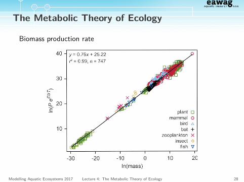
The Metabolic Theory of Ecology
Biomass production rate
Modelling Aquatic Ecosystems 2017 Lecture 4: The Metabolic Theory of Ecology 28
Chemical Equilibria
Chemical equilibria are important for
• the speciation of inorganic carbon, nitrogen and phosphoruscompounds,
• the precipitation and dissolution of calcite,
• the calculation of pH.
Modelling Aquatic Ecosystems 2017 Lecture 4: Chemical Processes 29
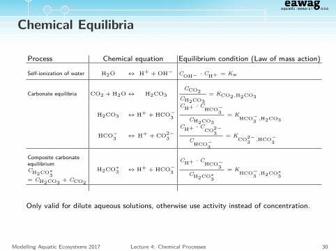
Chemical Equilibria
Process Chemical equation Equilibrium condition (Law of mass action)
Self-ionization of water H2O ↔ H+ + OH− COH− · CH+ = Kw
Carbonate equilibria CO2 + H2O↔ H2CO3CCO2
CH2CO3= KCO2,H2CO3
H2CO3 ↔ H+ + HCO−3
CH+ · CHCO−
3CH2CO3
= KHCO−
3 ,H2CO3
HCO−3 ↔ H+ + CO2−
3
CH+ · CCO2−
3C
HCO−3
= KCO2−
3 ,HCO−3
Composite carbonateequilibriumCH2CO∗
3= CH2CO3 + CCO2
H2CO∗3 ↔ H+ + HCO−
3
CH+ · CHCO−
3CH2CO∗
3
= KHCO−
3 ,H2CO∗3
Only valid for dilute aqueous solutions, otherwise use activity instead of concentration.
Modelling Aquatic Ecosystems 2017 Lecture 4: Chemical Processes 30
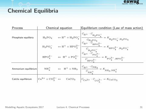
Chemical Equilibria
Process Chemical equation Equilibrium condition (Law of mass action)
Phosphate equilibria H3PO4 ↔ H+ + H2PO−4
CH+ · CH2PO−
4CH3PO4
= KH2PO−
4 ,H3PO4
H2PO−4 ↔ H+ + HPO2−
4
CH+ · CHPO2−
4C
H2PO−4
= KHPO2−
4 ,H2PO−4
HPO2−4 ↔ H+ + PO3−
4
CH+ · CPO3−
4C
HPO2−4
= KPO3−
4 ,HPO2−4
Ammonium equilibrium NH+4 ↔ H+ + NH3
CH+ · CNH3C
NH+4
= KNH3,NH+
4
Calcite equilibrium Ca2+ + CO2−3 ↔ CaCO3 CCa2+ · C
CO2−3
= KCaCO3
Modelling Aquatic Ecosystems 2017 Lecture 4: Chemical Processes 31
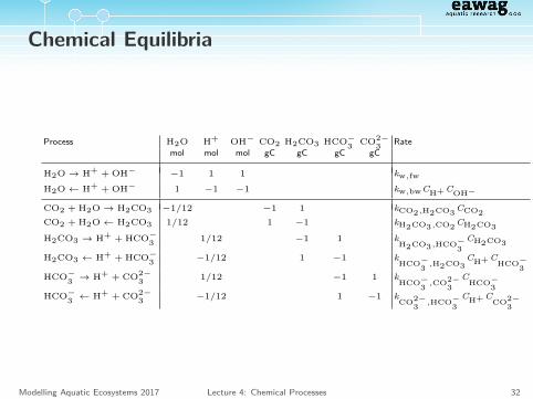
Chemical Equilibria
Process H2O H+ OH− CO2 H2CO3 HCO−3 CO2−
3 Ratemol mol mol gC gC gC gC
H2O→ H+ + OH− −1 1 1 kw,fw
H2O← H+ + OH− 1 −1 −1 kw,bwCH+ COH−
CO2 + H2O→ H2CO3 −1/12 −1 1 kCO2,H2CO3 CCO2CO2 + H2O← H2CO3 1/12 1 −1 kH2CO3,CO2 CH2CO3H2CO3 → H+ + HCO−
3 1/12 −1 1 kH2CO3,HCO−
3CH2CO3
H2CO3 ← H+ + HCO−3 −1/12 1 −1 k
HCO−3 ,H2CO3
CH+ CHCO−
3HCO−
3 → H+ + CO2−3 1/12 −1 1 k
HCO−3 ,CO2−
3C
HCO−3
HCO−3 ← H+ + CO2−
3 −1/12 1 −1 kCO2−
3 ,HCO−3
CH+ CCO2−
3
Modelling Aquatic Ecosystems 2017 Lecture 4: Chemical Processes 32
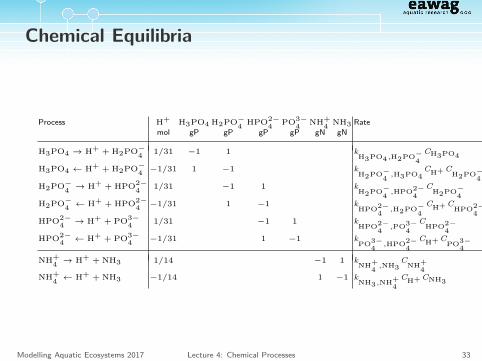
Chemical Equilibria
Process H+ H3PO4 H2PO−4 HPO2−
4 PO3−4 NH+
4 NH3 Ratemol gP gP gP gP gN gN
H3PO4 → H+ + H2PO−4 1/31 −1 1 k
H3PO4,H2PO−4
CH3PO4
H3PO4 ← H+ + H2PO−4 −1/31 1 −1 k
H2PO−4 ,H3PO4
CH+ CH2PO−
4H2PO−
4 → H+ + HPO2−4 1/31 −1 1 k
H2PO−4 ,HPO2−
4C
H2PO−4
H2PO−4 ← H+ + HPO2−
4 −1/31 1 −1 kHPO2−
4 ,H2PO−4
CH+ CHPO2−
4HPO2−
4 → H+ + PO3−4 1/31 −1 1 k
HPO2−4 ,PO3−
4C
HPO2−4
HPO2−4 ← H+ + PO3−
4 −1/31 1 −1 kPO3−
4 ,HPO2−4
CH+ CPO3−
4
NH+4 → H+ + NH3 1/14 −1 1 k
NH+4 ,NH3
CNH+
4NH+
4 ← H+ + NH3 −1/14 1 −1 kNH3,NH+
4CH+ CNH3
Modelling Aquatic Ecosystems 2017 Lecture 4: Chemical Processes 33
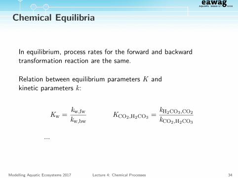
Chemical Equilibria
In equilibrium, process rates for the forward and backwardtransformation reaction are the same.
Relation between equilibrium parameters K andkinetic parameters k:
Kw = kw,fwkw,bw
KCO2,H2CO3 = kH2CO3,CO2
kCO2,H2CO3
...
Modelling Aquatic Ecosystems 2017 Lecture 4: Chemical Processes 34
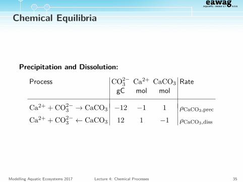
Chemical Equilibria
Precipitation and Dissolution:
Process CO2−3 Ca2+ CaCO3 Rate
gC mol mol
Ca2+ + CO2−3 → CaCO3 −12 −1 1 ρCaCO3,prec
Ca2+ + CO2−3 ← CaCO3 12 1 −1 ρCaCO3,diss
Modelling Aquatic Ecosystems 2017 Lecture 4: Chemical Processes 35
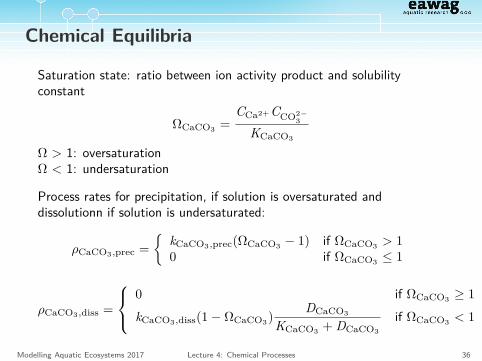
Chemical Equilibria
Saturation state: ratio between ion activity product and solubilityconstant
ΩCaCO3 =CCa2+CCO2−
3
KCaCO3
Ω > 1: oversaturationΩ < 1: undersaturation
Process rates for precipitation, if solution is oversaturated anddissolutionn if solution is undersaturated:
ρCaCO3,prec =
kCaCO3,prec(ΩCaCO3 − 1) if ΩCaCO3 > 10 if ΩCaCO3 ≤ 1
ρCaCO3,diss =
0 if ΩCaCO3 ≥ 1
kCaCO3,diss(1− ΩCaCO3) DCaCO3
KCaCO3 + DCaCO3
if ΩCaCO3 < 1
Modelling Aquatic Ecosystems 2017 Lecture 4: Chemical Processes 36
Sorption
Sorption of chemical substances to particles in the water columncan play an important role in aquatic systems.
Sorption of dissolved substances to sedimenting particles canincrease the elimination rate of substances from the water columnconsiderably.
Sorption is of particular interest for organic pollutants, heavymetals, and phosphate.
Modelling Aquatic Ecosystems 2017 Lecture 4: Chemical Processes 37
Sorption
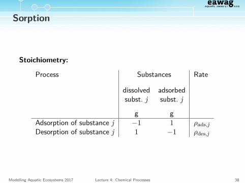
Stoichiometry:
Process Substances Rate
dissolved adsorbedsubst. j subst. j
g gAdsorption of substance j −1 1 ρads,jDesorption of substance j 1 −1 ρdes,j
Modelling Aquatic Ecosystems 2017 Lecture 4: Chemical Processes 38
Sorption
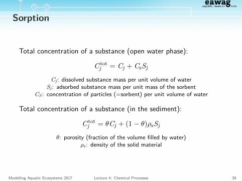
Total concentration of a substance (open water phase):
C totj = Cj + CsSj
Cj : dissolved substance mass per unit volume of waterSj : adsorbed substance mass per unit mass of the sorbent
CS : concentration of particles (=sorbent) per unit volume of water
Total concentration of a substance (in the sediment):
C totj = θCj + (1− θ)ρsSj
θ: porosity (fraction of the volume filled by water)ρs: density of the solid material
Modelling Aquatic Ecosystems 2017 Lecture 4: Chemical Processes 39
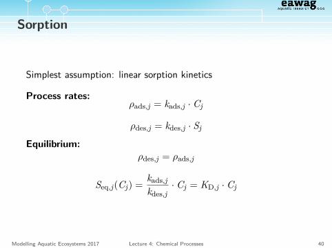
Sorption
Simplest assumption: linear sorption kinetics
Process rates:ρads,j = kads,j · Cj
ρdes,j = kdes,j · Sj
Equilibrium:ρdes,j = ρads,j
Seq,j(Cj) = kads,jkdes,j
· Cj = KD,j · Cj
Modelling Aquatic Ecosystems 2017 Lecture 4: Chemical Processes 40
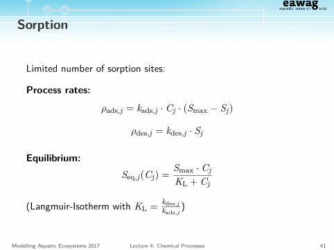
Sorption
Limited number of sorption sites:
Process rates:
ρads,j = kads,j · Cj · (Smax − Sj)
ρdes,j = kdes,j · Sj
Equilibrium:Seq,j(Cj) = Smax · Cj
KL + Cj
(Langmuir-Isotherm with KL = kdes,jkads,j
)
Modelling Aquatic Ecosystems 2017 Lecture 4: Chemical Processes 41
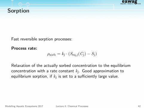
Sorption
Fast reversible sorption processes:
Process rate:ρsorb = kj · (Seq,j(Cj)− Sj)
Relaxation of the actually sorbed concentration to the equilibriumconcentration with a rate constant kj . Good approximation toequilibrium sorption, if kj is set to a sufficiently large value.
Modelling Aquatic Ecosystems 2017 Lecture 4: Chemical Processes 42
New Challenge: Develop your own model
During the semester you have to develop and implement your ownmodel (alone or in groups of two), interpret simulation results andperform a simple sensitivity analysis.
We provide two topics to choose from.We will assign topics on 29.03.2017 (now).
You will deliver the R-files and results by the end of the semester(2.6.2017!) per email to [email protected].
In the oral exam we will ask you about your example (beside othertopics).
Modelling Aquatic Ecosystems 2017 Lecture 4: Develop your own model 43
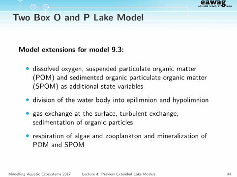
Two Box O and P Lake Model
Model extensions for model 9.3:
• dissolved oxygen, suspended particulate organic matter(POM) and sedimented organic particulate organic matter(SPOM) as additional state variables
• division of the water body into epilimnion and hypolimnion
• gas exchange at the surface, turbulent exchange,sedimentation of organic particles
• respiration of algae and zooplankton and mineralization ofPOM and SPOM
Modelling Aquatic Ecosystems 2017 Lecture 4: Preview Extended Lake Models 44
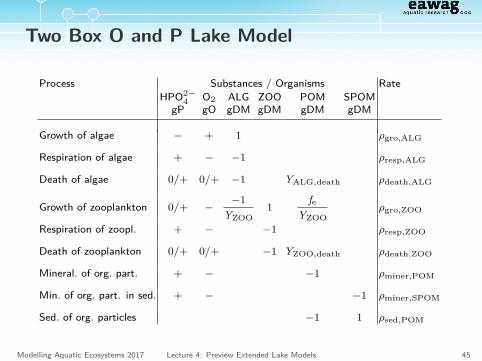
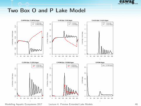
Two Box O and P Lake Model
Process Substances / Organisms RateHPO2−
4 O2 ALG ZOO POM SPOMgP gO gDM gDM gDM gDM
Growth of algae − + 1 ρgro,ALG
Respiration of algae + − −1 ρresp,ALG
Death of algae 0/+ 0/+ −1 YALG,death ρdeath,ALG
Growth of zooplankton 0/+ −−1
YZOO1
feYZOO
ρgro,ZOO
Respiration of zoopl. + − −1 ρresp,ZOO
Death of zooplankton 0/+ 0/+ −1 YZOO,death ρdeath,ZOO
Mineral. of org. part. + − −1 ρminer,POM
Min. of org. part. in sed. + − −1 ρminer,SPOM
Sed. of org. particles −1 1 ρsed,POM
Modelling Aquatic Ecosystems 2017 Lecture 4: Preview Extended Lake Models 45
Two Box O and P Lake Model
0 50 100 150 200 250 300 350
0.00
0.02
0.04
0.06
0.08
0.10
C.HPO4.Epi, C.HPO4.Hypo
t
C.H
PO
4.E
pi, C
.HP
O4.
Hyp
o
C.HPO4.EpiC.HPO4.Hypo
0 50 100 150 200 250 300 350
05
1015
2025
C.O2.Epi, C.O2.Hypo
t
C.O
2.E
pi, C
.O2.
Hyp
o
C.O2.EpiC.O2.Hypo
0 50 100 150 200 250 300 350
01
23
45
67
C.ALG.Epi, C.ALG.Hypo
t
C.A
LG.E
pi, C
.ALG
.Hyp
o
C.ALG.EpiC.ALG.Hypo
0 50 100 150 200 250 300 350
0.0
0.2
0.4
0.6
0.8
C.ZOO.Epi, C.ZOO.Hypo
t
C.Z
OO
.Epi
, C.Z
OO
.Hyp
o
C.ZOO.EpiC.ZOO.Hypo
0 50 100 150 200 250 300 350
0.0
0.5
1.0
1.5
2.0
C.POM.Epi, C.POM.Hypo
t
C.P
OM
.Epi
, C.P
OM
.Hyp
o
C.POM.EpiC.POM.Hypo
0 50 100 150 200 250 300 350
05
1015
2025
D.POM.Hypo
t
D.P
OM
.Hyp
o
D.POM.Hypo
Modelling Aquatic Ecosystems 2017 Lecture 4: Preview Extended Lake Models 46
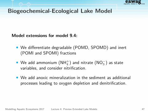
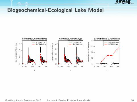
Biogeochemical-Ecological Lake Model
Model extensions for model 9.4:
• We differentiate degradable (POMD, SPOMD) and inert(POMI and SPOMI) fractions
• We add ammonium (NH+4 ) and nitrate (NO−
3 ) as statevariables, and consider nitrification.
• We add anoxic mineralization in the sediment as additionalprocesses leading to oxygen depletion and denitrification.
Modelling Aquatic Ecosystems 2017 Lecture 4: Preview Extended Lake Models 47
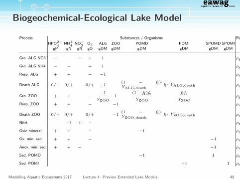
Biogeochemical-Ecological Lake Model
Process Substances / Organisms RateHPO2−
4 NH+4 NO−
3 O2 ALG ZOO POMD POMI SPOMD SPOMIgP gN gN gO gDM gDM gDM gDM gDM gDM
Gro. ALG NO3 − − + 1 ρgro,ALG,NO3
Gro. ALG NH4 − − + 1 ρgro,ALG,NH4
Resp. ALG + + − −1 ρresp,ALG
Death ALG 0/+ 0/+ 0/+ −1 (1 − fI)·YALG,death
fI· YALG,death ρdeath,ALG
Gro. ZOO + + −−1
YZOO1
(1− fI)fe
YZOO
fIfe
YZOOρgro,ZOO
Resp. ZOO + + − −1 ρresp,ZOO
Death ZOO 0/+ 0/+ 0/+ −1 (1 − fI)·YZOO,death
fI· YZOO,death ρdeath,ZOO
Nitri. −1 + − ρnitri
Oxic mineral. + + − −1 ρminer,ox,POM
Ox. min. sed. + + − −1 ρminer,ox,SPOM
Anox. min. sed. + + − −1 ρminer,anox,SPOM
Sed. POMD −1 1 ρsed,POMD
Sed. POMI −1 1 ρsed,POMI
Modelling Aquatic Ecosystems 2017 Lecture 4: Preview Extended Lake Models 48
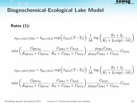
Biogeochemical-Ecological Lake Model
Rates (1):
ρgro,ALG,NH4 = kgro,ALG·exp(βALG(T−T0)
)· 1λh log
(KI + I0
KI + I0 exp(−λh)
)
·min(
CHPO4
KHPO4 + CHPO4,
CNH4 + CNO3
KN + CNH4 + CNO3
)· pNH4CNH4
pNH4CNH4 + CNO3·CALG
ρgro,ALG,NO3 = kgro,ALG·exp(βALG(T−T0)
)· 1λh log
(KI + I0
KI + I0 exp(−λh)
)
·min(
CHPO4
KHPO4 + CHPO4,
CNH4 + CNO3
KN + CNH4 + CNO3
)· CNO3
pNH4CNH4 + CNO3·CALG
Modelling Aquatic Ecosystems 2017 Lecture 4: Preview Extended Lake Models 49
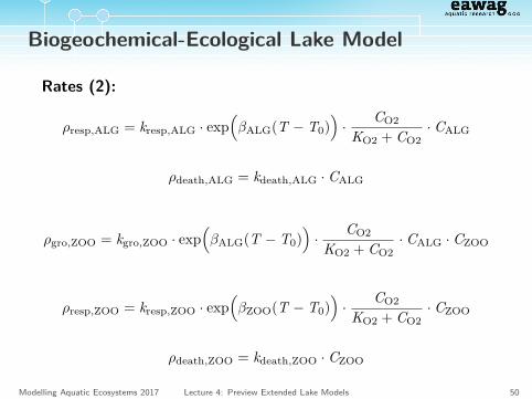
Biogeochemical-Ecological Lake Model
Rates (2):
ρresp,ALG = kresp,ALG · exp(βALG(T − T0)
)· CO2
KO2 + CO2· CALG
ρdeath,ALG = kdeath,ALG · CALG
ρgro,ZOO = kgro,ZOO · exp(βALG(T − T0)
)· CO2
KO2 + CO2· CALG · CZOO
ρresp,ZOO = kresp,ZOO · exp(βZOO(T − T0)
)· CO2
KO2 + CO2· CZOO
ρdeath,ZOO = kdeath,ZOO · CZOO
Modelling Aquatic Ecosystems 2017 Lecture 4: Preview Extended Lake Models 50
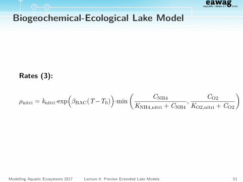
Biogeochemical-Ecological Lake Model
Rates (3):
ρnitri = knitri·exp(βBAC(T−T0)
)·min
(CNH4
KNH4,nitri + CNH4,
CO2
KO2,nitri + CO2
)
Modelling Aquatic Ecosystems 2017 Lecture 4: Preview Extended Lake Models 51
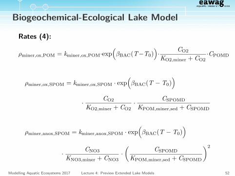
Biogeochemical-Ecological Lake Model
Rates (4):
ρminer,ox,POM = kminer,ox,POM·exp(βBAC(T−T0)
)· CO2
KO2,miner + CO2·CPOMD
ρminer,ox,SPOM = kminer,ox,SPOM · exp(βBAC(T − T0)
)· CO2
KO2,miner + CO2· CSPOMD
KPOM,miner,sed + CSPOMD
ρminer,anox,SPOM = kminer,anox,SPOM · exp(βBAC(T − T0)
)· CNO3
KNO3,miner + CNO3·(
CSPOMD
KPOM,miner,sed + CSPOMD
)2
Modelling Aquatic Ecosystems 2017 Lecture 4: Preview Extended Lake Models 52
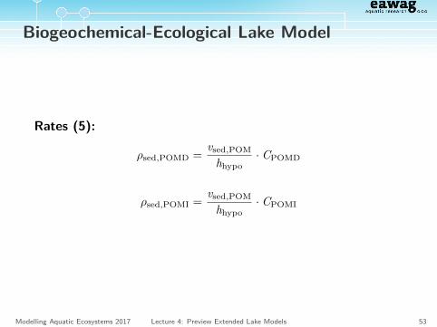
Biogeochemical-Ecological Lake Model
Rates (5):
ρsed,POMD = vsed,POM
hhypo· CPOMD
ρsed,POMI = vsed,POM
hhypo· CPOMI
Modelling Aquatic Ecosystems 2017 Lecture 4: Preview Extended Lake Models 53
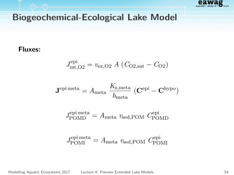
Biogeochemical-Ecological Lake Model
Fluxes:
J epiint,O2 = vex,O2 A (CO2,sat − CO2)
Jepi meta = AmetaKz,metahmeta
(Cepi −Chypo)
J epi metaPOMD = Ameta vsed,POM C epi
POMD
J epi metaPOMI = Ameta vsed,POM C epi
POMI
Modelling Aquatic Ecosystems 2017 Lecture 4: Preview Extended Lake Models 54
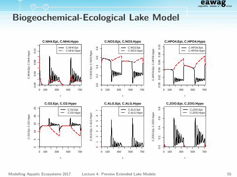
Biogeochemical-Ecological Lake Model
0 100 300 500 700
0.00
0.04
0.08
0.12
C.NH4.Epi, C.NH4.Hypo
t
C.N
H4.
Epi
, C.N
H4.
Hyp
o
C.NH4.EpiC.NH4.Hypo
0 100 300 500 700
0.0
0.2
0.4
0.6
0.8
C.NO3.Epi, C.NO3.Hypo
t
C.N
O3.
Epi
, C.N
O3.
Hyp
o
C.NO3.EpiC.NO3.Hypo
0 100 300 500 700
0.00
0.02
0.04
0.06
0.08
0.10
C.HPO4.Epi, C.HPO4.Hypo
t
C.H
PO
4.E
pi, C
.HP
O4.
Hyp
o
C.HPO4.EpiC.HPO4.Hypo
0 100 300 500 700
05
1015
2025
C.O2.Epi, C.O2.Hypo
t
C.O
2.E
pi, C
.O2.
Hyp
o
C.O2.EpiC.O2.Hypo
0 100 300 500 700
01
23
45
67
C.ALG.Epi, C.ALG.Hypo
t
C.A
LG.E
pi, C
.ALG
.Hyp
o
C.ALG.EpiC.ALG.Hypo
0 100 300 500 700
0.0
0.2
0.4
0.6
0.8
C.ZOO.Epi, C.ZOO.Hypo
t
C.Z
OO
.Epi
, C.Z
OO
.Hyp
o
C.ZOO.EpiC.ZOO.Hypo
0 100 300 500 700
0.0
0.5
1.0
1.5
C.POMD.Epi, C.POMD.Hypo
t
C.P
OM
D.E
pi, C
.PO
MD
.Hyp
o C.POMD.EpiC.POMD.Hypo
0 100 300 500 700
0.0
0.1
0.2
0.3
0.4
C.POMI.Epi, C.POMI.Hypo
t
C.P
OM
I.Epi
, C.P
OM
I.Hyp
o
C.POMI.EpiC.POMI.Hypo
0 100 300 500 700
010
2030
40
D.POMD.Hypo, D.POMI.Hypo
t
D.P
OM
D.H
ypo,
D.P
OM
I.Hyp
o D.POMD.HypoD.POMI.HypoModelling Aquatic Ecosystems 2017 Lecture 4: Preview Extended Lake Models 55
Biogeochemical-Ecological Lake Model
0 100 300 500 700
0.00
0.04
0.08
0.12
C.NH4.Epi, C.NH4.Hypo
t
C.N
H4.
Epi
, C.N
H4.
Hyp
o
C.NH4.EpiC.NH4.Hypo
0 100 300 500 700
0.0
0.2
0.4
0.6
0.8
C.NO3.Epi, C.NO3.Hypo
t
C.N
O3.
Epi
, C.N
O3.
Hyp
o
C.NO3.EpiC.NO3.Hypo
0 100 300 500 700
0.00
0.02
0.04
0.06
0.08
0.10
C.HPO4.Epi, C.HPO4.Hypo
t
C.H
PO
4.E
pi, C
.HP
O4.
Hyp
o
C.HPO4.EpiC.HPO4.Hypo
0 100 300 500 700
05
1015
2025
C.O2.Epi, C.O2.Hypo
t
C.O
2.E
pi, C
.O2.
Hyp
o
C.O2.EpiC.O2.Hypo
0 100 300 500 700
01
23
45
67
C.ALG.Epi, C.ALG.Hypo
t
C.A
LG.E
pi, C
.ALG
.Hyp
o
C.ALG.EpiC.ALG.Hypo
0 100 300 500 700
0.0
0.2
0.4
0.6
0.8
C.ZOO.Epi, C.ZOO.Hypo
t
C.Z
OO
.Epi
, C.Z
OO
.Hyp
o
C.ZOO.EpiC.ZOO.Hypo
0 100 300 500 700
0.0
0.5
1.0
1.5
C.POMD.Epi, C.POMD.Hypo
t
C.P
OM
D.E
pi, C
.PO
MD
.Hyp
o C.POMD.EpiC.POMD.Hypo
0 100 300 500 700
0.0
0.1
0.2
0.3
0.4
C.POMI.Epi, C.POMI.Hypo
t
C.P
OM
I.Epi
, C.P
OM
I.Hyp
o
C.POMI.EpiC.POMI.Hypo
0 100 300 500 700
010
2030
40
D.POMD.Hypo, D.POMI.Hypo
t
D.P
OM
D.H
ypo,
D.P
OM
I.Hyp
o D.POMD.HypoD.POMI.Hypo
Modelling Aquatic Ecosystems 2017 Lecture 4: Preview Extended Lake Models 56
Exercises
1. Introduction to R and the ecosim package.Demonstration of the implementation of a simple lakephytoplankton model.
2. Phytoplankton-zooplankton model for a mixed lake.
3. Practice of stoichiometric calculations.Introduction to the stoichcalc package.
4. Two box lake model for plankton and biogeochemical cycles.
5. River benthos and water column model with sessile algae andbacteria and O, P and N cycles
6. Consideration of environmental stochasticity and uncertainty.
Modelling Aquatic Ecosystems 2017 Lecture 4: Outlook 57
Outlook Lecture 5
• Physical processes in Lakes
• Mass balance in multibox systems
• Mass balance in continuous systems
• Transport and mixing in lakes
• Sedimentation, gas exchange
Modelling Aquatic Ecosystems 2017 Lecture 4: Outlook 58