MODELLING AND SIMULATION OF WIND SPEED …tariq/deepa.pdfMODELLING AND SIMULATION OF WIND SPEED AND...

MODELLING AND SIMULATION OF WIND SPEED AND

WIND FARM POWER PREDICTION

Presenter: Deepa Paga Supervisor: Dr. Tariq Iqbal

Co- supervisor: Prof. Andy Fisher Faculty of Engineering and Applied Science

Memorial University of Newfoundland 25th July, 2013

1

Outline

 Wind Speed and Wind Farm Power Models Overview  Short Term Wind Speed Prediction Using ARMA Model  An Hour Ahead Wind Speed Prediction Using Kalman

Filter and Unscented Kalman Filter  Power Prediction of the Fermeuse Newfoundland Wind

Farm  Power Prediction of the Cedar Creek, Colorado Wind

Farm  Conclusion   Future Work

2

Wind Speed and Wind Farm Power Models Overview

•  Wind Speed Forecasting Models •  Persistence Model •  Auto Regressive Model (AR Model) •  Auto Regressive and Moving Average (ARMA Model) •  Autoregressive Integral and Moving Average (ARIMA) •  Artificial Neural Network •  Neural Network •  Numerical Weather Prediction Model •  Hybrid Model

3

Physical Factors Effecting Wind Turbine Power Production

Horizontal Shear Topography Vertical Shear Complex Terrain Direction Shear Dust Pressure Temperature Turbulence Icing Wake Effect Air Density Humidity

4

Short Term Wind Speed Prediction Using ARMA Model

 ARMA Model  Mathematical Model of ARMA Model  Simulated Results of ARMA Model

5

Mathematics of the ARMA Model

•  ARMA(1,1) model is given as: y(t) + a1y(t-1) = e(t) + c1e(t-1) •  AR (1) model has the form of a regression model in

which y(t) is regressed on its previous value. •  In moving average (MA) model the time series is

regarded as a moving average or unevenly weighted random series e(t).

•  e(t), e(t-1) are the residuals at times t and t-1. •  c1 is the first-order moving average coefficient. •  a1 is the autoregressive coefficient.

6

MATLAB Simulated Result of the ARMA Model

Input Hourly Wind Speed Data.

Predicted Hourly Five Hours In advance Wind Speed Data.

7

Comparison of the actual and the predicted wind speed data in km/hr and time in hours.

Comparison of Actual and Predicted Wind Speed

Wind Data Statistics Actual Wind Speed Data (m/s)

Predicted Wind Speed Data (m/s)

Mean 5.55 4.88 Median 5.27 4.81 Standard Deviation 2.21 2.11

8

An Hour Ahead Wind Speed Prediction Using Kalman Filter and Unscented

Kalman Filter •  In the wind speed prediction part, an Auto Regressive

model and a non linear Auto Regressive Exogenous model is used for a short term wind speed prediction to predict an hourly average wind speed up to 1 hour in advance.

•  The Kalman filter and the Unscented Kalman Filter are used for filtering associated noise in the input wind speed for accurate estimation.

•  The Kalman filter is used for linear system •  Unscented Kalman filter for the non linear system.

9

•  System Identification toolbox is used for processing the input wind speed.

•  For the Kalman filter, the input wind speed is processed using the Auto Regressive model of order 2 from the linear parametric toolbox.

•  For the Unscented Kalman Filter, the input wind speed is processed using the Non linear ARX model of order 2.

•  State space of AR model is used for Kalman filter as the initial condition for the matrix.

•  State space of non linear ARX model is used for Unscented Kalman filter as the initial condition for the matrix.

•  More details of algorithm given in the thesis.

10

Simulated MATLAB Results of the Wind Speed Data

Input wind speed is plotted with respect to time. Input wind speed has 2/3rd data as training data (green) and 1/3rd data as validation data (red).

11

Best fitted one step ahead wind speed data tested with AR model and the ARMA model of different model order in the system identification toolbox.

Non Linear ARX model compared with various model orders

12

The Kalman Filter and the Unscented Kalman Filter State Estimation

Properly tuned Kalman filter wind speed estimation. Kalman filter estimation with increase in measurement noise.

13

Kalman filter estimation with increase in process noise (Qf) and the measurement noise (Rf) remaining constant.

Process noise and measurement noise is reduced with UKF properly tuned.

14

UKF performance with increase in process noise.

UKF performance with increase in measurement noise.

15

Power Prediction of the Fermeuse Newfoundland Wind Farm

•  The Fermeuse wind farm is located in the community of the Fermeuse on the Southern Shore, Avalon Peninsula in Newfoundland.

•  The wind farm has nine wind turbines in an operating condition.

•  The wind turbine used at the Fermeuse wind farm is the Vestas V90 3MW, and the wind farm capacity is 27MW.

16 Fermeuse

Overview of the Wind Power Model  Wind Turbine Power Estimation •  Turbulence Intensity •  Vertical Shear •  Pressure •  Temperature •  Air Density   Wind Farm Power Estimation •  Speed and Height of each wind turbine varies •  Wind Farm Layout •  Wind Direction  Other Factors •  MET Tower, Hub Height, and Radius of Wind Turbine

17

  Requirement •  Manufacturer supplied power curve, Wind Turbine

Specifications. •  Input: Pressure, Temperature, Air density, Wind Speed,

Wind Direction •  Wind Data: Given in every 10 minutes 10,000 data set in

time series order. •  Output: Corrected power curve of wind turbine •  Software used: MS Excel, MATLAB

18

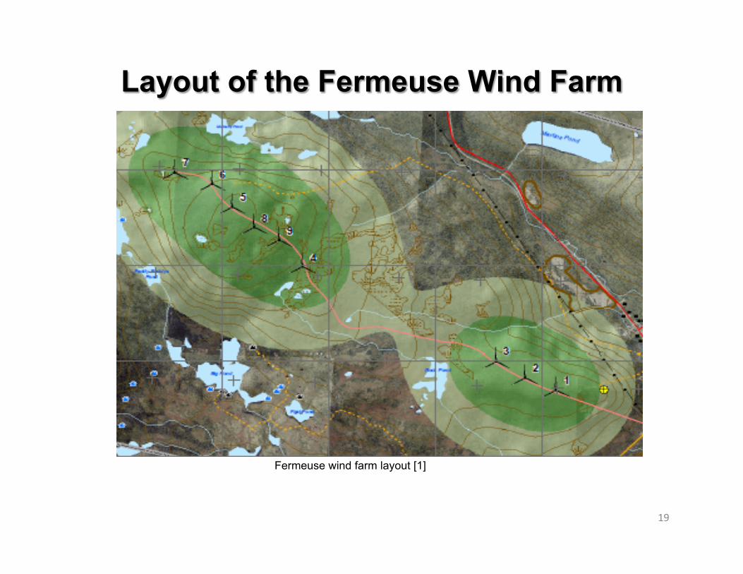
Layout of the Fermeuse Wind Farm

Fermeuse wind farm layout [1]

19

  Wind Turbines at the Fermeuse Site. Wind turbines at the Fermeuse wind farm [3]

20

Designed Algorithm of Wind Power Physical Model

•  Digitizing manufacturer supplied power curve. •  Uncorrected Power Curve Equation

•  Wind speed is determined from lower wind turbine rotor tip to upper wind turbine rotor tip.

21

•  Turbulence intensity (Iu) is determined from the given input wind speed (WS) and standard deviation data (σ) at certain heights of wind turbine rotor disc.

•  Turbulence adjusted wind speed (U') is determined at the given model level at certain heights of wind turbine rotor disc using input wind speed (U) and turbulence intensity (Iu) at the model levels intersecting wind turbine rotor disc.

•  Wind shear exponent ‘α’ is determined from the turbulence adjusted wind speed (U') at certain heights(H1, H2) of wind turbine rotor disc.

22

•  Disc speed (Udisk) adjusted for turbulence and vertical shear is determined from lower rotor tip (H–R) to upper rotor tip(H+R) of wind turbine by solving for Uz using the power law equation of shear.

•  Air density correction is applied to the uncorrected power curve equation (Puncorr) and corrected power curve (Pcorr) of wind turbine is determined. Pcorr = Puncorr *Actual Density/ Density at STP

Actual Density = 3.4837 * Pressure/Temperature Density at STP = 1.225 kg/m^3

23

Wake Effect in Fermeuse Wind Farm •  Wind power of a wind turbine is reduced at a particular

wind direction in the wind farm. tanα = 0.04 (free stream) / 0.08(wake stream)

24

Fermeuse Wind Farm Estimated Data

Specification of the Vestas V90, 3MW Wind Turbine.

Specifications of the Wind Turbine

Vestas V90 3MW Wind Turbine

Cut in wind speed 3.5 m/s

Rated wind speed 15 m/s

Rotor Diameter 90 m

Rated Power 3.0 MW

Hub Height 80m

Cut out wind speed 25 m/s

26

Four sets of input wind speed data are used.

Wind power of a wind turbine-2 in the wind farm using the input wind data file1.

Average Value of Physical Factors of Wind Power Model considered from the Designed Algorithm

Estimated Average Power of Vestas V 90, 3 MW Wind Turbine

Vertical shear at hub height 1.43 MW Turbulence adjusted speed at hub height

2.15 MW

Estimated disc speed at hub height

1.86 MW

Estimated air density adjusted disc speed

1.91 MW

27

Wake coefficient data determined from the wind direction and shadow effect of the wind turbines in the Fermeuse wind farm.

Time Series Wind Speed Data of Equal Length (10 min)

Wind Direction (45o ±50; 225o ± 50)

All other Wind Direction (except 450± 50 ; 2250± 50)

W.C of Wind Data 1 0.84 1.00 W.C of Wind Data 2 0.85 1.00

W.C of Wind Data 3 0.83 1.00


28

Estimated power output of the Fermeuse wind farm.


Average Wind Farm Power of Vestas V 90 Wind Turbines(3 MW- 9 WT)

Wind Data 1 17.34 MW Wind Data 2 18.76 MW Wind Data 3 16.26 MW Wind Data 4 11.16 MW

29

Transmission Loss

  Transmission Loss in the Wind farm: It occurs due to the current flow in the cables and there is reduction in power.

  The transmission loss is about 1%. (ref ?)   The loss factor is multiplied with the total power of the

wind farm.

30

Estimated Fermeuse wind farm power before and after transmission loss (TL) in wind farm.

Input Wind Data

TL Average Wind Farm Power before TL (No-wake)

Average Wind Farm Power after TL (No-wake)

Average Wind Farm Power before TL (Wake)

Average Wind Farm Power after TL (Wake)

Wind Data1

1.0% 17.34 MW 17.16 MW 16.37 MW 16.20 MW

Wind Data2

1.0% 18.76 MW 18.57 MW 17.84 MW 17.66 MW

Wind Data3

1.0% 16.26 MW 16.10 MW 15.32 MW 15.16 MW

Wind Data4

1.0% 11.16 MW 11.04 MW 10.29 MW 10.18 MW

31

Estimated Loss in the power of the Fermeuse wind farm due to power transmission.

Time Series Input Wind Speed Data of Equal Length (10 min)

Transmission Loss

Loss in Power (No wake effect)

Loss in Power (Wake effect)

Wind Data 1 1.0% 0.17 MW 0.16 MW Wind Data 2 1.0% 0.19 MW 0.18 MW Wind Data 3 1.0% 0.16 MW 0.15 MW Wind Data 4 1.0% 0.12 MW 0.10 MW

32

Simulated MATLAB Results of Fermeuse Wind Farm

Recorded sensor height wind speed data for the Vestas V90, 3MW

wind turbine-2. (Note: Time Scale: X axis: 1 unit =10 minute; 1000 unit = 10000 minutes).

Hub height wind speed is estimated for the Vestas V90 3MW wind turbine-2 at the hub height. (Note: Time Scale: X axis: 1 unit =10 minute; 1000 unit = 10000 minutes).

33

Turbulence adjusted wind speed estimated for the Vestas V90 3MW wind turbine-2 at the hub height. (Note: Time Scale: X axis: 1 unit =10 minute; 1000 unit = 10000 minutes).

Estimated disc speed adjusted for turbulence and shear for the Vestas V90 3 MW wind turbine-2 at the hub height. (Note: Time Scale: X axis: 1 unit =10 minute; 1000 unit = 10000

minutes).

34

Wake speed estimated for Vestas 3 MW wind turbine-2 at hub height (Note: Time Scale: X axis: 1 unit =10 minute; 1000 unit = 10000 minutes).

Estimated power curve of the Vestas 3MW wind turbine adjusted with air density.

35

Comparison of the wind power of the wind turbine -2 operating at the wake effect (black) and no wake effect (red).

Comparison of estimated wind farm power with the wake effect (red) and without wake effect (black) is plotted

with respect to time. (Note: Time Scale: X axis: 1 unit =10 minute; 1000 unit = 10000 minutes).

36

Wind direction (degrees) at the wind farm site for a time span of 10,000 minutes. (Note: Time Scale: X axis: 1 unit =10 minute; 1000 unit = 10000 minutes).

Wake coefficient determined from the wind direction is plotted with respect to time.

(Note: Time Scale: X axis: 1 unit =10 minute; 1000 unit = 10000 minutes).

37

Power Prediction of the Cedar Creek,

Colorado Wind farm

•  The Cedar Creek wind farm is located in the United States. The wind farm has 274 wind turbines in an operating condition.

•  The wind turbines of the Cedar Creek-I wind farm are the 221, Mitsubishi 1MW and 53, GE 1.5MW wind turbines and the total capacity of the wind farm is 300MW.

•  The designed algorithm estimates the wind speed adjusted for shear and turbulence for the wind turbine rotor disc from the lower rotor tip to the upper rotor tip of the wind turbine.

•  The value estimated is the effective wind speed and is assumed to be at the hub height.

•  Air density is adjusted to predict the wind power of each wind turbine.

38

•  The speed and height for each wind turbine varies when estimating power for the wind farm.

•  It depends on the distance between the wind turbines, the contour height and the layout information.

•  The wake model is incorporated when the wind turbines are located at a closer distance.

•  The wake power of the wind farm is estimated considering the wind direction, the wind farm layout information, the thrust coefficient of the wind turbine, and the free disc speed.

39

Layout Information of Cedar Creek Colorado Wind Farm

Cedar Creek- I Wind farm Layout [4].

A section of the Cedar Creek Wind farm Layout [4].

40

Designed Algorithm of the Cedar Creek Wind Farm

The manufacturer supplied power curve of the GE 1.5MW wind turbine and the Mitsubishi 1.0 MW wind turbine is digitized by plotting power vs. wind speed characteristics.

For the GE 1.5MW wind turbine Here s= Estimated disc speed value of the GE 1.5 MW wind turbine

41

For the Mitsubishi 1MW wind turbine Here r = Estimated disc speed value of the Mitsubishi 1 MW wind

turbine. Hub height wind speed of the wind turbine is given by

42

The turbulence intensity (Iu) at a known heights is calculated using from an input wind speed (U) at a MET tower height of 69m and 80m for Mitsubishi 1MW and GE 1.5MW wind turbine respectively and using standard deviation data (σ) of the input wind speed.

The turbulence adjusted wind speed (U’ (TI)) is calculated from the input wind speed and the turbulence intensity (Iu) for the Mitsubishi 1MW and the GE 1.5 MW wind turbine.

43

Wind shear exponent,’α’ is calculated using power law equation of shear.

The wind velocity across the wind turbine rotor disc

which is adjusted for turbulence and vertical shear is determined from the lower rotor tip (H-R) to the upper rotor tip (H+R) of the wind turbine.

44

•  Air density correction is applied to the uncorrected power curve equation (Puncorr) and corrected power curve (Pcorr) of a wind turbine is determined.

•  Actual Density = 3.4837 * Pressure/Temperature •  Density at STP = 1.225 kg/m^3

Pcorr = Puncorr *Actual Density/Density at STP Where P(uncorr) = GP(uncorr) for the GE wind turbine and MP

(uncorr) for the Mitsubishi wind turbine. P(corr) =GP(corr) for the GE wind turbine and MP(corr) for the

Mitsubishi wind turbine.

45

Wake Effect in the Wind Farm

Wake Effect in a Wind farm [2] .

•  Depending on the distance between the wind turbines (X), the radius of the shadow cone Rx of the upstream turbine is calculated from the radius of rotor (R) and tanα.

tanα = 0.04 (free stream) / 0.08(wake stream)

46

•  Wind power of a wind farm with the wake effect •  The thrust coefficient (Ct) of the wind turbine is

calculated from the disc speed adjusted for vertical shear and turbulence. The disc speed is assumed to be at the hub height of the wind turbine.

47

•  The wake speed (Uwake) of a wind turbine is calculated from the disc speed, the thrust coefficient, the radius of the rotor disc, the radius of the shadow cone (Rx) of rotor disc, the area of shadow region (AS) of rotor disc and the area of the wind turbine rotor (A).

•  The uncorrected wake power of the wind turbine is

calculated for the GE 1.5MW and the Mitsubishi 1 MW wind turbine respectively

48

•  For the Mitsubishi 1MW Wind Turbine •  Uncorrected power is adjusted with air density and wind

power is determined under the influence of wake effect.

49

Here P1(uncorr_wake) = GP(uncorr_wake) for GE wind turbine

and MP(uncorr_wake) for Mitsubishi wind turbine. P1(corr_wake) = GP(corr_wake) for the GE wind turbine and MP(corr_wake) for the Mitsubishi wind turbine.

Wind power of a wind farm with the wake effect. Wake coefficient of a wind turbines in the wind farm

50

Cedar Creek Wind Farm Estimated Data

Specifications of the Wind Turbines

Specifications of Wind Turbine

G.E. 1.5 MW wind turbine

Mitsubishi 1 MW wind turbine

Rated wind speed 12.5 m/s 12 m/s Rotor Diameter 77 m 61.4 m Rated Power 1.5 MW 1.0 MW Hub Height 80 m 69 m Cut out wind speed

25 m/s 25 m/s

51

Wind power of a wind turbine-2 in the wind farm using the input wind data file1.

Average Value of Physical Factors of Wind Power Model considered from the Designed Algorithm

Estimated Average Power of GE 1.5 MW Wind Turbine

Estimated Average Power of Mitsubishi 1 MW Wind Turbine

Vertical shear at hub height

628.86 KW 272 KW

Turbulence adjusted speed at hub height

1.148 MW 633.09 KW

Estimated disc speed at hub height

1.124 MW 617.87 KW

Estimated air density adjusted disc speed

1.15 MW 632.1 KW

52

Wake coefficient data determined from the wind direction and shadow effect of the wind turbines in the wind farm.


Wind Direction (45o ±50; 225o

±50)

All other Wind Direction (except 450± 50; 2250± 50)

W.C of Wind Data 1 0.8451 1.0 W.C of Wind Data 2 0.8452 1.0



53

Estimated power output of the Cedar Creek Colorado wind farm.


G.E Wind Turbines (1.5 MW- 53 WT)

Mitsubishi Wind Turbines (1MW-221 WT)

Average Wind Farm Power. (GE + Mitsubishi)

Wind Data 1 49.10 MW 111.4 MW 160.5 MW Wind Data 2 49.34 MW 112.1 MW 161.3 MW Wind Data 3 49.55 MW 112.29 MW 161.7 MW Wind Data 4 49.50 MW 112.19 MW 161.6 MW

54

Estimated Colorado wind farm power before and after the transmission loss (TL) in wind farm.

Input Wind Data

TL Average Wind Farm Power before TL (No-wake)

Average Wind Farm Power after TL (No-wake)

Average Wind Farm Power before TL (Wake)

Average Wind Farm Power after TL (Wake)

Wind Data1

1.0% 160.51 MW 158.89 MW 135.63 MW 134.27 MW

Wind Data2

1.0% 161.31 MW 159.68 MW 136.33 MW 134.97 MW

Wind Data3

1.0% 161.71 MW 160.08 MW 136.49 MW 135.12 MW

Wind Data4

1.0% 161.64 MW 160.03 MW 136.41 MW 135.05 MW

55

Estimated Loss in the power of the Colorado wind farm due to power transmission.

Time Series Input Wind Speed Data of Equal Length (10 min)

Transmission Loss

Loss in Power (No wake effect)

Loss in Power (Wake effect)

Wind Data 1 1.0% 1.605 MW 1.356 MW Wind Data 2 1.0% 1.613 MW 1.3633 MW Wind Data 3 1.0% 1.6172 MW 1.3649 MW Wind Data 4 1.0% 1.616 MW 1.364 MW

56

Simulated Results of the designed algorithm to estimate wind farm power

Power vs. Wind Speed characteristics of Mitsubishi 1 MW wind turbine (supplied power curve).

Power vs. Wind Speed characteristics of GE 1.5 MW wind turbine (supplied power curve).

57

Power vs. Wind Speed characteristics of Mitsubishi1 MW wind turbine (curve fitted).

Power vs. Wind Speed characteristics of GE 1.5 MW wind turbine (curve fitted).

58

Sensor height wind speed data for the GE 1.5 MW wind turbine-2 recorded

from MET tower1. (Note: Time Scale: X axis: 1 unit =10 minute; 1000 unit = 10000 minutes).

Sensor height wind speed data for the Mitsubishi 1.0 MW wind turbine-2 recorded from MET tower2.


59

Hub height wind speed estimated for the GE 1.5 MW wind turbine-2. (Note: Time Scale: X axis: 1 unit =10 minute; 1000 unit = 10000 minutes).

Hub height wind speed estimated for the Mitsubishi 1MW wind turbine- 2. (Note: Time Scale: X axis: 1 unit =10 minute; 1000 unit = 10000 minutes). 60

Turbulence adjusted wind speed estimated for GE 1.5 MW wind turbine- 2 at hub height. (Note: Time Scale: X axis: 1 unit =10 minute; 1000 unit = 10000 minutes).

Turbulence adjusted wind speed estimated for Mitsubishi 1.0 MW wind turbine-2 at hub

height. (Note: Time Scale: X axis: 1 unit =10 minute; 1000 unit = 10000 minutes).

61

Estimated disc Speed (adjusted for turbulence and shear) for GE 1.5 MW wind turbine-2 at hub height. (Note: Time Scale: X axis: 1 unit =10 minute; 1000 unit = 10000 minutes).

Estimated disc speed (adjusted for turbulence and shear) for Mitsubishi 1.0 MW wind

turbine-2 at hub height. (Note: Time Scale: X axis: 1 unit =10 minute; 1000 unit = 10000 minutes).

62

Wake speed estimated for GE 1.5 MW wind turbine-2 at hub height (Note: Time Scale: X axis: 1 unit =10 minute; 1000 unit = 10000 minutes).

Wake speed estimated for Mitsubishi 1.0 MW wind turbine-2 at hub height. (Note: Time Scale: X axis: 1 unit =10 minute; 1000 unit = 10000 minutes).

63

Estimated power curve of GE 1.5 MW wind turbine-1 adjusted with air density.

Estimated power curve of the Mitsubishi 1MW wind turbine-1 adjusted with air density.

64

Comparison of power estimated with wake (black) and without wake (red) effect for GE 1.5 MW wind turbine-2. (Note: Time Scale: X axis: 1 unit =10 minute; 1000 unit = 10000 minutes).

Comparison of power estimated with wake (black) and without wake (red) effect for Mitsubishi 1.0 MW wind

turbine-2. (Note: Time Scale: X axis: 1 unit =10 minute; 1000 unit = 10000 minutes).

65

Comparison of estimated wind farm power with wake effect (red) and no-wake effect (black) with respect to time. (Note: Time Scale: X axis: 1 unit =10 minute; 1000 unit = 10000 minutes).

Wind direction (degrees) at the wind farm site for a time span of 5000 minutes. (Note: Time

Scale: X axis: 1 unit =10 minute; 1000 unit = 10000 minutes).

66

Wake coefficient determined from wind direction is plotted with respect to time (Note: Time Scale: X axis: 1 unit =10 minute; 1000 unit = 10000 minutes).

Wind farm output power with power loss (1%) in transmission with no wake effect is plotted with respect to time. (Note: Time Scale: X axis: 1 unit =10 minute; 1000 unit = 10000 minutes).

67

Wind farm output power with power loss (1%) in transmission and wake effect is plotted with respect to time.


68

Actual estimated wind farm power with transmission loss of 1% due to wake effect is plotted with respect to time. (Note: Time Scale: X axis: 1 unit =10 minute; 1000 unit = 10000 minutes).

Actual estimated wind farm power with transmission loss of 1% with no wake effect is plotted with respect

to time (Note: Time Scale: X axis: 1 unit =10 minute; 1000 unit = 10000 minutes).

69

Conclusion   The major contributing factors in the wind power

production and their effect on the wind power estimation is determined.

  The combined effect of the physical factors such as vertical shear, turbulence intensity, air density has a major effect on the wind turbine energy production.

  The wind farm layout, the influence of the wind direction, the thrust coefficient of the wind turbine, and the wind turbine placements in the wind farm have a greater influence in determining the wake coefficient data and the wind farm efficiency in the wind farm.

 ARMA model gives accurate result for short term wind prediction.

70

Conclusion (continued.....)  A wind speed predictor has been developed and

simulated in Matlab.  A Mathematical power output model of Feremuse wind

farm has been developed and tested for four data sets.  A Mathematical power output model of Colorado Cedar

Creek Wind Farm has be developed and tested for four site recorded data sets.

71

Future Work

  The future research work on the wind speed forecasting requires forecasting days ahead or a week ahead wind speed from Numerical Weather Prediction model.

  In the wind power forecasting, the future work should focus on the effect of atmospheric humidity, the effect of turbulent kinetic energy, and horizontal shear which has a major contribution in the wind power estimation from the wind turbines.

  The effect of icing conditions and the ice accumulation on the wind turbine rotor blades has a greater influence in the wind power generation. The future work should focus on de-icing techniques under severe icing conditions.

72

Acknowledgment

  Dr. Tariq Iqbal   Prof. Andy Fisher   Michael Abbott, David Bryan and project members of

AMEC Earth and Environment, St John’s, NL   School of Graduate Studies (SGS), Memorial University

of Newfoundland.   Map Room, Queen Elizabeth II Library, Memorial

University of Newfoundland.   My family and friends

73

Some References

•  [1] Fermeuse wind farm layout information: Retrieved from http://www.env.gov.nl.ca.

•  [2] The wake effect, Retrieved from http://www.algonquinadventures.com/waywardwind/thewind.htm

•  [3] Vestas wind turbine picture taken at the site visit to the Fermeuse wind farm, Newfoundland.

•  [4] Arc Geographic Information System, Cedar Creek layout map: Map Room, Queen Elizabeth II Library, Memorial University of Newfoundland.

74

Publications •  Submitted report on real time prediction of a wind farm

power output for Mitacs Accelerate Program. (Scholarship was awarded for the period September 2011 to December 2011 as MITACS intern researcher at AMEC Earth and Environment, St John’s)

•  Deepa Paga, Dr. T. Iqbal, “Power Prediction of a Wind Farm in the Fermeuse, Newfoundland,” presented at IEEE-NECEC Conference 8th November, 2012 at St. John’s, NL.

•  Deepa Paga, Dr. T. Iqbal, “Short Term Wind Speed Prediction Using ARMA Model,” presented at Aldrich Conference April, 2013 at St. John’s, NL.

75

Thank You

76

MODELLING AND SIMULATION OF WIND SPEED …tariq/deepa.pdfMODELLING AND SIMULATION OF WIND SPEED AND...

Documents

Transcript of MODELLING AND SIMULATION OF WIND SPEED …tariq/deepa.pdfMODELLING AND SIMULATION OF WIND SPEED AND...