Modelling and forecasting monthly Brent crude oil prices ...

STATISTICS IN TRANSITION new series, March 2021 Vol. 22, No. 1 pp. 29–54, DOI 10.21307/stattrans-2021-002 Received – 31.12.2019; accepted – 07.09.2020

Modelling and forecasting monthly Brent crude oil prices: a long memory and volatility approach

Remal Shaher AlـGounmeein1, Mohd Tahir Ismail2

ABSTRACT

The Standard Generalised Autoregressive Conditionally Heteroskedastic (sGARCH) model and the Functional Generalised Autoregressive Conditionally Heteroskedastic (fGARCH) model were applied to study the volatility of the Autoregressive Fractionally Integrated Moving Average (ARFIMA) model, which is the primary objective of this study. The other goal of this paper is to expand on the researchers' previous work by examining long memory and volatilities simultaneously, by using the ARFIMA-sGARCH hybrid model and comparing it against the ARFIMA-fGARCH hybrid model. Consequently, the hybrid models were configured with the monthly Brent crude oil price series for the period from January 1979 to July 2019. These datasets were considered as the global economy is currently facing significant challenges resulting from noticeable volatilities, especially in terms of the Brent crude prices, due to the outbreak of COVID-19. To achieve these goals, an R/S analysis was performed and the aggregated variance and the Higuchi methods were applied to test for the presence of long memory in the dataset. Furthermore, four breaks have been detected: in 1986, 1999, 2005, and 2013 using the Bayes information criterion. In the further section of the paper, the Hurst Exponent and Geweke-Porter-Hudak (GPH) methods were used to estimate the values of fractional differences. Thus, some ARFIMA models were identified using AIC (Akaike Information Criterion), BIC (Schwartz Bayesian Information Criterion), AICc (corrected AIC), and the RMSE (Root Mean Squared Error). In result, the following conclusions were reached: the ARFIMA(2,0.3589648,2)-sGARCH(1,1) model and the ARFIMA(2,0.3589648,2)-fGARCH(1,1) model under normal distribution proved to be the best models, demonstrating the smallest values for these criteria. The calculations conducted herein show that the two models are of the same accuracy level in terms of the RMSE value, which equals 0.08808882, and it is this result that distinguishes our study. In conclusion, these models can be used to predict oil prices more accurately than others. Key words: ARFIMA, volatility, fGARCH, sGARCH, modelling and forecasting, hybrid model.

1 Corresponding author. School of Mathematical Sciences, Universiti Sains Malaysia, Pulau Pinang, Malaysia and

Department of Mathematics, Faculty of Science, AlـHussein Bin Talal University, Ma'an, Jordan. E-mail: [email protected]. ORCID: https://orcid.org/0000-0002-2415-6937.

2 School of Mathematical Sciences, Universiti Sains Malaysia, Pulau Pinang, Malaysia. E-mail: [email protected]. ORCID: https://orcid.org/0000-0003-2747-054X.

30 R. S. Al-Gounmeein, M. T. Ismail: Modelling and forecasting monthly…

1. Introduction

Over the years, the study of oil price and volatility has remained one of the most important economic trends in terms of increasing investment and minimizing risk. Therefore, it is necessary to use an accurate statistical method to know the changes in price in terms of increase and decrease, through what is known as long memory (Mostafaei and Sakhabakhsh, 2012).

Long memory is a phenomenon we may sometimes face when analysing the time series data where long-term dependence between two points increases the amount of distance between them (Bahar et al., 2017). Usually when modelling long memory behaviour for any time series, such as mathematics, economics, among others; the operation can be more accurate by relying on the Autoregressive Fractionally Integrated Moving Average (ARFIMA) models compared with Autoregressive Integrated Moving Average (ARIMA) models. It can also have an important impact in the financial field (Bhardwaj and Swanson, 2006), where long memory models are one of the most important models used in the analysis of time series (Karia et al., 2013). ARFIMA model was fitted for the time series data either to better understand the data or to predict the future points in the series (forecasting). The use of forecasting in economic and financial fields is very important at the national, regional and international levels. It helps investors to reduce financial risks and increase the profits in the volatility of the global economy. The ARFIMA model was created by Granjer and Joyeux (1980) as mentioned by Mostafaei and Sakhabakhsh (2012) to capture the long memory behaviour of this time series data. The long memory feature exists if the autocorrelation function (ACF) decays more slowly than the exponential decay described by Bahar et al. (2017) or detected by using the statistical methods, namely Hurst Exponent as explained in Beran (1994). Besides, it is a known fact that long memory characteristics observed in data can be generated by a nonstationary structural break, as mentioned by Ohanissian et al. (2008). Therefore, the importance of testing for structural breaks in the conditional mean of a time series is necessary, as it determines that long memory is real or fake, as pointed out by Diebold and Inoue (2001), Granger and Hyung (2004) and Ohanissian et al. (2008). Therefore, the break detection procedure exhibits desirable properties both in the presence of breaks (stable potency across multiple breaks), as pointed out in Pretis et al. (2016). Besides, performing structural break testing when estimating the ARFIMA model is of great importance as it increases accuracy and prediction confidence.

On the other hand, volatility is an important consideration for any time series, especially in oil prices. Volatility is noticeable in studies related to financial, economic, tourism and other areas, where the data is widely scattered (Tendai and Chikobvu, 2017; Akter and Nobi, 2018). As it is known, there are obvious volatilities shown in some types of time series especially in crude oil prices (Lee and Huh, 2017). Therefore,

STATISTICS IN TRANSITION new series, March 2021

31

it was necessary to study these volatilities to avoid inaccuracies in the development of plans and strategies for making important decisions or for future predictions necessary. Moreover, to know their impact when forecasting to avoid any financial risks that may cause losses to the investor as the forecasting of financial time series data is yet as one of the most difficult tasks due to the non-stationary and non-linearity, as studied by Ismail and Awajan (2017). Also, Ramzan et al. (2012) showed that one category of models which has confirmed successful in forecasting volatility in many cases is the GARCH family of models. This is studied here by Standard Generalized Autoregressive Conditionally Heteroskedastic (sGARCH) model and Functional Generalized Autoregressive Conditionally Heteroskedastic (fGARCH) model. Based on the reason above we are choosing to study the long memory and volatility in this study, due to the modality of Brent crude oil prices grow exponentially, nonstationary and are volatile. These phenomena are popular features found in many large-scale data.

2. Literature review

For many years, many studies have been published that relate to the modelling and forecasting crude oil price (Yu et al., 2008; Aamir and Shabri, 2015; Sehgal and Pandey, 2015; Bahar et al., 2017; Lee and Huh, 2017; Yu et al., 2017; He, X. J., 2018; Yin et al., 2018). One of the old studies was by Yu et al. (2008), where they proposed using an empirical mode decomposition that depends on the learning model of the neural network group. The experimental results showed that the proposed model is a very capable approach to predicting international crude oil prices. Later, Aamir and Shabri (2015) used Auto-regressive Integrated Moving Average (ARIMA), Generalized Auto-regressive Conditional Heteroscedasticity (GARCH) and hybrid ARIMA-GARCH for modelling and forecasting monthly crude oil price of Pakistan. They found that the ARIMA-GARCH model is suitable and perform best based on the value of Akaike's Information Criterion (AIC) and Root Mean Squared Error (RMSE). Meanwhile, Sehgal and Pandey (2015) showed that Artificial Intelligent methods widely use forecasting oil prices as an alternative to traditional methods. Then, Lee and Huh (2017) suggested an alternative model which predicts the oil price using a Bayesian approach with informative priors. While Yu et al. (2017) found that Support Vector Machine (SVM) model outperformed Feed-Forward Neural Networks (FNN), Auto-Regressive Integrated Moving Average (ARIMA) model, Fractional Integrated ARIMA (ARFIMA) model, Markov-Switching ARFIMA (MS-ARFIMA) model, and Random Walk (RW) model for forecasting one-step or multi-step of crude oil price. In contrast, Bahar et al. (2017) used West Texas Intermediate daily data from 2/January/1986 to 31/August/2016, where the result showed that the price of crude oil has structural breaks feature. Moreover, the forecasting result showed high accuracy with geometric Brownian motion when compared with the mean-reverting Ornstein-Uhlenbeck


process for the short term. In 2018, He, X. J. identified the appropriate model for crude oil price prediction among several models used for weekly price data during the period 2009-2017. Machine learning Support Vector Regression (SVR) was found the best model. On the other hand, Yin et al. (2018) used numerous predictor variables with a new time-varying weight combination method where the results showed strong performance in forecasting the oil price.

Recently, many authors such as Fazelabdolabadi (2019) and Nyangarika et al. (2019) have still been interested in oil price prediction in terms of choosing the best predictive model. Nyangarika et al. (2019) used exponential smoothing to modify an Auto-Regressive Integrated Moving Average (ARIMA) model for the Brent crude oil price and Gas price data during the period from Jan/1991 to Dec/2016. In contrast, Fazelabdolabadi (2019) proposed the forecasting of the crude oil prices by applying a hybrid Bayesian Network (BN) method. The results showed that the proposed method is a good choice for short-term forecasting.

As mentioned previously, several models were used for modelling and forecasting the price of crude oil. The ARFIMA model is one of the famous models used in the analysis of time series (Karia et al., 2013) and understands the behaviour of the data, specifically crude oil prices. Jibrin et al. (2015) also used the ARFIMA model to study and forecast crude oil prices using weekly West Texas Intermediate and Brent series for the period 15/5/1987 to 20/12/2013, and explained that the WTI series and the Brent series have three breaks in the years 1999, 2004, 2008 and 1999, 2005, 2009, respectively. Bahar et al. (2017) used West Texas Intermediate daily data from 2/January/1986 to 31/August/2016, and the result showed that the price of crude oil had structural breaks feature. Also, there are previous studies that used volatility and hybrid models to describe the movement of crude oil prices. Hybrid models are an important method for studying the relationship between long memory and volatility. Among these studies, Manera et al. (2004) estimated the dynamic conditional correlations in the returns on Tapis oil spot and one-month forward prices for the period from 2 June 1992 to 16 January 2004, using CCCMGARCH (Constant Conditional Correlation Multivariate GARCH) model, VARMAGARCH (Vector Autoregressive Moving Average GARCH) model, VARMA-AGARCH (VARMA–Asymmetric GARCH) model, and DCC (Dynamic Conditional Correlation) model. The result shows that the ARCH and GARCH effects for spot (forward) returns are significant in the conditional volatility model for spot (forward) returns. Moreover, the multivariate asymmetric effects are significant for both spot and forward returns. Also, the calculated constant conditional correlations between the conditional volatilities of spot and forward return are virtually identical using CCC-GARCH(1,1), VAR(1)-GARCH(1,1) and VAR(1)-AGARCH(1,1). After that, in (2013) Kang and Yoon examined the volatility models and their forecasting abilities for three types of petroleum futures contracts traded on the New York Mercantile Exchange (West Texas Intermediate crude oil, heating oil #2,


33

and unleaded gasoline) particularly regarding volatility persistence (or long-memory properties). These models are ARIMA–GARCH, ARFIMA–GARCH, ARFIMA–IGARCH, and ARFIMA–FIGARCH. Although the ARFIMA–FIGARCH model better captures long-memory characteristics of returns and volatility, the out-of-sample analysis indicates that there is no single model for all three types of petroleum futures contracts, and this calls on investors to exercise caution when measuring and forecasting volatility (risk) in petroleum futures markets. As for Akron and Ismail (2017), they proposed a hybrid GA-FEEMD (Genetic Algorithm and Fast Ensemble Empirical Mode Decomposition) model for forecasting crude oil price time-series data. The results showed that the proposed hybrid model improved the forecasting accuracy of the data, compared with ARIMA and artificial neural network methods. On the other hand, Daniel Ambach and Oleksandra Ambach (2018) conducted a study on the application of a periodic regression model with the ARFIMA-GARCH residual process to model and predict the oil price, whereas the hybrid model provided some advantages, including that it captures long memory and conditional heteroscedasticity, but it failed to capture the periodicity in a good way. Besides, for the first lag of the squared standardized residuals, the proposed model showed a remaining presence of correlation, which is not satisfying at all. Therefore, it should be extended.

As a summary, previous studies have shown that there are mixed results in terms of selecting the appropriate model for the modelling and forecasting of crude oil prices. Thus, the current study focuses on constructing a time series model to forecast the monthly Brent crude oil price using ARFIMA with the GARCH family approach. Furthermore, due to the lack of studies in which crude oil prices have been predicted by comparing the ARFIMA-sGARCH hybrid model versus the ARFIMA-fGARCH hybrid model. Also, it will extend the works in the previous literature by examining long memory and volatilities in Brent crude oil prices simultaneously, by using the comparison of these models: ARFIMA-sGARCH model versus the ARFIMA-fGARCH model. Finally, this study also focuses on the interest in taking the two smallest values for accuracy criteria such as AIC and not just one value when choosing the best model. Thus, these points will be highlighted in this study. So, the purpose of this work is to identify structural breaks, verify that long memory is present for monthly Brent crude oil price data. Then, to determine the best model among ARFIMA models using some criteria and accuracy measures, such as AIC (Akaike information criterion) and RMSE (root mean squared error) in the sample. Besides, to check the residuals of the model for the existence of volatility or not, to determine the optimal model that can be used to study conditional variation (volatility) in series data through sGARCH and fGARCH models, to obtain the best hybrid model to predict the price of Brent crude oil in the short-term with the smallest error value.


3. Materials and Methods

3.1. The Dataset

Monthly data of the Brent crude oil price (all prices are per barrel in USA $) were used in this study from January 1979 to July 2019, obtained from the website: www.indexmundi.com/commodities/?commodity=crude-oil-brent. The data were divided into two parts: the first included data from January 1979 to July 2018 consisting of 475 observations, which were used to fit the forecasting model; while the second part has data from August 2018 to July 2019 consisting of 12 observations, which were used to test the accuracy of the in-sample forecast. Thereafter, a 13-month prediction was carried out outside the sample. This study uses the R-software version (3.5.3) to implement all statistical analyses.

3.2. Long Memory Test and Estimation

To check the presence of the long memory feature, there are several statistical methods that can be used, as described in Boutahar et al. (2007). These methods are R/S analysis, the aggregated variance method, and the Higuchi method. In particular, the range over standard deviation (R/S) analysis, which is a diagnostic of long memory, was the role played by Mandelbrot (1972), then Lo (1991) modified it. Mandelbrot (1972) found that the R/S analysis shows good properties over autocorrelation function (ACF) analysis and variance time function (VTF) analysis. After that, Lo (1991) modified R/S analysis, it is robust to short-range dependence, non-normal distributions, and conditional heteroscedasticity under the null hypothesis of no long-term dependence. This analysis achieves the following formula, as shown by Mandelbrot (1972) and Lo (1991):

𝑄 ∑ ∑

∑ (1)

where 𝑋 𝑛 ∑ 𝑋 (2) and (𝑛) is the sample size.

Besides, Jibrin et al. (2015) mentioned that a single structural break test is a test to determine the presence of break. It was introduced by Chow (1960) and modified to the Quandt Likelihood Ratio (QLR) test for the break between (𝑡 and 𝑡 ) or called the Supremum F-statistic, given by:

𝑆𝑢𝑝 𝐹 max 𝐹 𝑡 , 𝐹 𝑡 1 , … , 𝐹 𝑡 (3) where if Supremum F-statistic > 0.05, then the test rejects the null hypothesis which is 𝐻 : no structural breaks.


35

On the other hand, the value of the fractional difference (𝑑) was estimated by several methods, which were illustrated by (Hosking, 1981; Reisen, 1994; Boutahar et al., 2007; Palma, 2007; Telbany and Sous, 2016). These methods are:

The Hurst Exponent method: Reisen (1994) mentioned that this method, proposed by Hurst (1951, 1956) and then reviewed by McLeod and Hipel (1978), is based on the range (𝑅∗ ) of the subtotals to deviate values from their mean in the time series divided by the standard deviation (𝐷∗ ), which is denoted by (𝑅 ) and written as follows:

𝑅∗

∗ ∑ ∑

∑ (4)

where 𝑋 𝑛 ∑ 𝑋 (5) The Geweke and Porter-Hudak (GPH) method: Based on the regression equation

𝑌 , Geweke and Porter-Hudak (1983) suggested the estimation for the parameter (𝑑 ), according to the following equations:

𝑑 ∑ 𝑋 𝑋 ∑ 𝑋 𝑋 𝑌 𝑌 (6) where 𝑌 𝛼 𝛽𝑋 𝜀 (7)

𝑌 𝑛 ∑ 𝑌 (8) In contrast, the smoothed periodogram (Sperio) and fractionally-differenced

(Fracdiff) are just functions in R-software, used to estimate the value of the fractional difference (d), according to the following formulas respectively:

Reisen (1994) clarified the Sperio function, which estimates the fractional difference (d) in the ARFIMA(p,d,q) model. This function, represented by 𝑓 𝑤 and that is through the Parzen lag window, is as follows:

𝑓 𝑤 ∑ 𝐿 𝑅 𝑠 cos 𝑠𝑤 (9)

where L 𝑢1 6𝑢 6|𝑢| , |𝑢| 1 2⁄2 1 |𝑢| , 1 2⁄ 𝑢 1 0 , |𝑢| 1

(10)

L 𝑢 is called the Parzen lag window generator (we select the Parzen lag window as it has the feature that always yields positive estimates of the spectral density), c is the parameter (commonly indicated to the ‘truncation point’) and

𝑅 s ∑ 𝑋 𝑋 𝑋 𝑋 , 𝑠 0, 1, … , 𝑛 1 (11)

indicate the sample autocovariance function. Hosking (1981) defined the fractionally-differenced operator, which uses the

regression estimation method to estimate the fractional difference (d) for the ARFIMA


model (Olatayo and Adedotun, 2014). The (d) value is calculated by a binomial series, as follows:

∇ 1 𝐵𝑑𝑘

𝐵

1 𝑑𝐵12

𝑑 1 𝑑 𝐵16

𝑑 1 𝑑 2 𝑑 𝐵 ⋯

(12)

3.3. Models Specification

The definitions of the ARIMA model were proposed by Box and Jenkins (Box et al., 2008) as follows. A stationary time series }{ tx is called an Autoregressive Integrated Moving Average model of order ( qdp ,, ) denoted by ( ),,( qdpARIMA ), if

𝜙 𝐵 ∇ 𝑥 𝜃 𝐵 𝜖 (13) whereas, )....1()( 2

21p

pp BBBB (14)

)...1()( 221

qqq BBBB (15)

dd B)1( (16) where )(Bp is a polynomial of autoregressive for order 𝑝 denoted by AR(p);

)(Bq is a polynomial of moving average for order 𝑞 denoted by MA(q). The integer number 𝑑 is the non-seasonal difference order. 𝐵 are the backward shift operators defined by ktt

k XXB . ∇ are the non-seasonal difference operators. Furthermore, 𝜖 is a white noise process.

ARFIMA model is the same as the ARIMA model above, but the essence of the difference between them is in the value of 𝑑 . If 𝑑 ∈ 0, 0.5 , then the data has a long memory. While intermediate memory if 𝑑 ∈ 0.5,0 . However, when 𝑑 0, then the data has a short memory (for mathematical details, see Beran (1994) page 60).

3.4. GARCH Models

In 1986, Bollerslev expanded the Autoregressive Conditional Heteroscedasticity (ARCH) model with order 𝑞 , which Engle developed in 1982, to become the Generalised Autoregressive Conditional Heteroscedasticity (GARCH) model with order 𝑝, 𝑞 (Francq and Zakoian, 2019). The first model depends on uncorrelated random error values 𝜀 . In contrast, the GARCH model relies on conditional variation. The general form of the 𝐺𝐴𝑅𝐶𝐻 𝑝, 𝑞 model is given by Francq and Zakoian (2019) as follows:

𝜀 𝜂 𝜎 , 𝑤𝑖𝑡ℎ 𝜂 𝑁 0,1~ (17)

𝜎 𝜔 ∑ 𝛼 𝜀 ∑ 𝛽 𝜎 (18)


37

where 𝜔 0 , 𝛼 0 𝑎𝑛𝑑 𝛽 0 𝑎𝑟𝑒 𝑐𝑜𝑛𝑠𝑡𝑎𝑛𝑡𝑠, 𝑖 1,2, … 𝑞, 𝑗 1,2, … 𝑝,𝑎𝑛𝑑 𝑡 ∈ ℤ. Whereas when 𝛽 0, then equation (18) is called 𝐴𝑅𝐶𝐻 𝑞 . In contrast, if 𝑝 𝑞 0, then equation (18) becomes white noise. When the conditional variance of the process is unknown, the Asymptotic Quasi-likelihood (AQL) methodology is merging the kernel technique to estimate the parameter of the GARCH model, such as in Alzghool (2017).

3.5. Standard GARCH (sGARCH) Model

The conditional variance 𝜎 at a time 𝑡 is expressed by the standard GARCH (p,q) model, the same as the equation (18), where 𝜀 is considered the residual returns, as the equation (17), which have been mentioned above (Miah and Rahman, 2016).

3.6. Functional GARCH (fGARCH) Model

Given the urgent need to describe the high-frequency volatilities that abound in the financial statements, a proper rational description of this problem, known as the function, had to be found (Francq and Zakoian, 2019). In 2013, Hörmann et al. suggested the functional approach of the ARCH model, then expanded this approach in 2017 by Aue et al., as mentioned by Francq and Zakoian (2019), through focusing on fGARCH(1,1) process such as in Aue et al. (2017), as shown below:

𝜎 𝛿 α𝜀 β𝜎 (19)

where 𝜀 is a sequence of random functions satisfying the equation (17), 𝛿 0, 𝛼0 , 𝛽 0 𝑎𝑛𝑑 𝑖 ∈ ℤ.

Note that for 𝑡 ∈ 0,1 and 𝑥 is an arbitrary element of the Hilbert space ℋ𝐿 0,1 , the integral operators 𝛼 𝑎𝑛𝑑 𝛽 are defined by 𝛼𝑥

𝛼 𝑡, 𝑠 𝑥 𝑠 𝑑𝑠 and 𝛽𝑥 𝛽 𝑡, 𝑠 𝑥 𝑠 𝑑𝑠. The integral kernel functions α 𝑡, 𝑠 and β 𝑡, 𝑠 are elements on 𝐿 0,1 .

As mentioned above, their approach depends on a daily division of the data (Francq and Zakoian, 2019), with the possibility for other time units (Aue et al., 2017), for example a monthly time unit, (see Aue et al., 2017; Francq and Zakoian, 2019 for more details).

3.7. Hybrid ARFIMA-GARCH Models

If the variance of the 𝐴𝑅𝐹𝐼𝑀𝐴 𝑝, 𝑑, 𝑞 model can be modelled by a 𝐺𝐴𝑅𝐶𝐻 𝑝, 𝑞 process, then this model is to be termed a hybrid 𝐴𝑅𝐹𝐼𝑀𝐴 𝑝, 𝑑, 𝑞 GARCH p, q . This model was defined by Palma (2007) as follows:

𝜙 𝐵 ∇ 𝑥 𝜃 𝐵 𝜀 (20)


where 𝜀 𝜂 𝜎 , 𝑤𝑖𝑡ℎ 𝜂 𝑁 0,1~ (21)

𝜎 𝜔 ∑ 𝛼 𝜀 ∑ 𝛽 𝜎 (22)

According to the above, each model of the hybrid models will be estimated 𝐴𝑅𝐹𝐼𝑀𝐴 𝑝, 𝑑, 𝑞 𝑠𝐺𝐴𝑅𝐶𝐻 𝑝, 𝑞 and 𝐴𝑅𝐹𝐼𝑀𝐴 𝑝, 𝑑, 𝑞 𝑓𝐺𝐴𝑅𝐶𝐻 𝑝, 𝑞 under different distributions. Namely, normal (norm) distribution, student’s t (std) distribution and generalized error (ged) distribution, see Tendai and Chikobvu (2017).

3.8. Criteria and Accuracy Measures for Choosing the Best Model

The fit model selection among several models is based on many criteria such as Akaike Information Criterion (AIC), Schwartz Bayesian Information Criterion (BIC) and corrected AIC (AICc) as indicated by Cryer and Chan (2008). They are given by the following formulas:

𝐴𝐼𝐶 2 ln 𝑙 2𝑘 (23)

𝐵𝐼𝐶 2 ln 𝑙 𝑘𝑙𝑛 𝑛 (24)

𝐴𝐼𝐶𝑐 2 ln 𝑙 2𝑘 (25)

where 𝑙 is a maximum likelihood for the model, 𝑘 is the total number of parameters 𝑚𝑒𝑎𝑛𝑖𝑛𝑔 𝑘 𝑝 𝑞 through the equations (14) and (15) respectively, while 𝑛 is

the number of observations. Therefore, the best model which gives the lowest value for these AIC, BIC and AICc criteria. Furthermore, the Root Mean Square Error (RMSE) is one of the accuracy measures which is used for evaluation of the performance of the model, as explained by Montgomery et al. (2015), as follows:

𝑅𝑀𝑆𝐸 ∑ 𝑌 𝑌 (26)

where 𝑌 is the actual value and 𝑌 is the forecasted value.

4. Results and Discussion

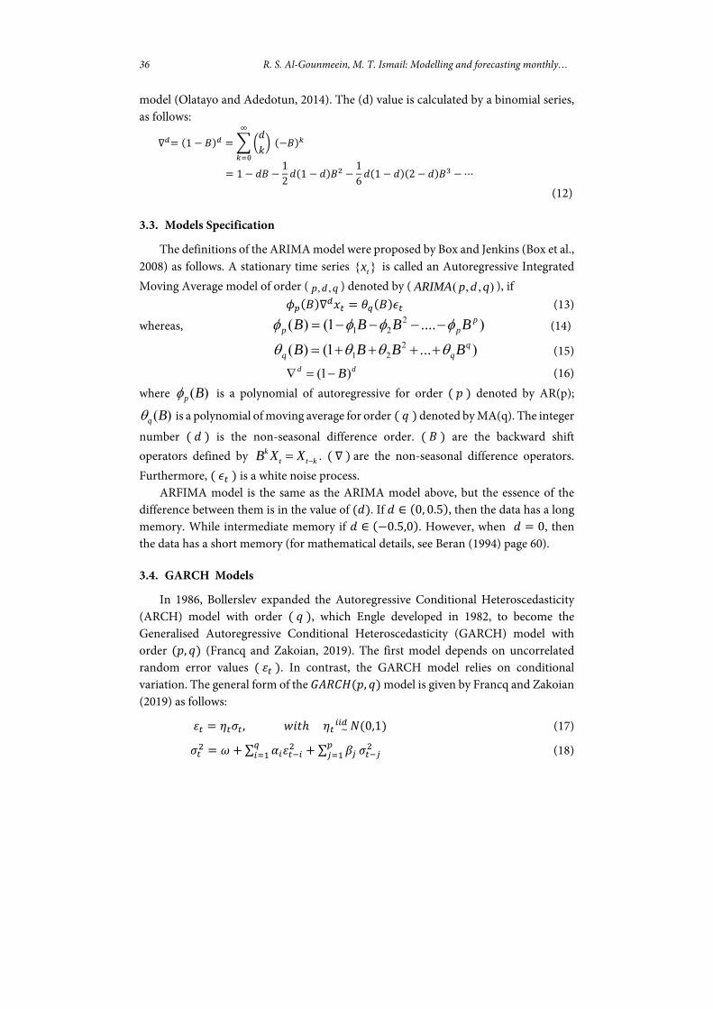
The monthly Brent crude oil price series is denoted by {𝑋 and 𝑡 represents the time in months. Figure 1 displays the time series plot 𝑋 for the dataset from January 1979 to July 2019. Through the 𝑋 series, large fluctuations are observed over time, especially in 2008. The descriptive statistics of the monthly Brent crude oil price that consists of 487 observations have a mean of 42.95, a median of 30.20 and a positive skewness of 1.177466. For this reason, the tail of the series is on the left side.


39

Figure 1. Time series plot for monthly Brent crude oil price ($/bbl)

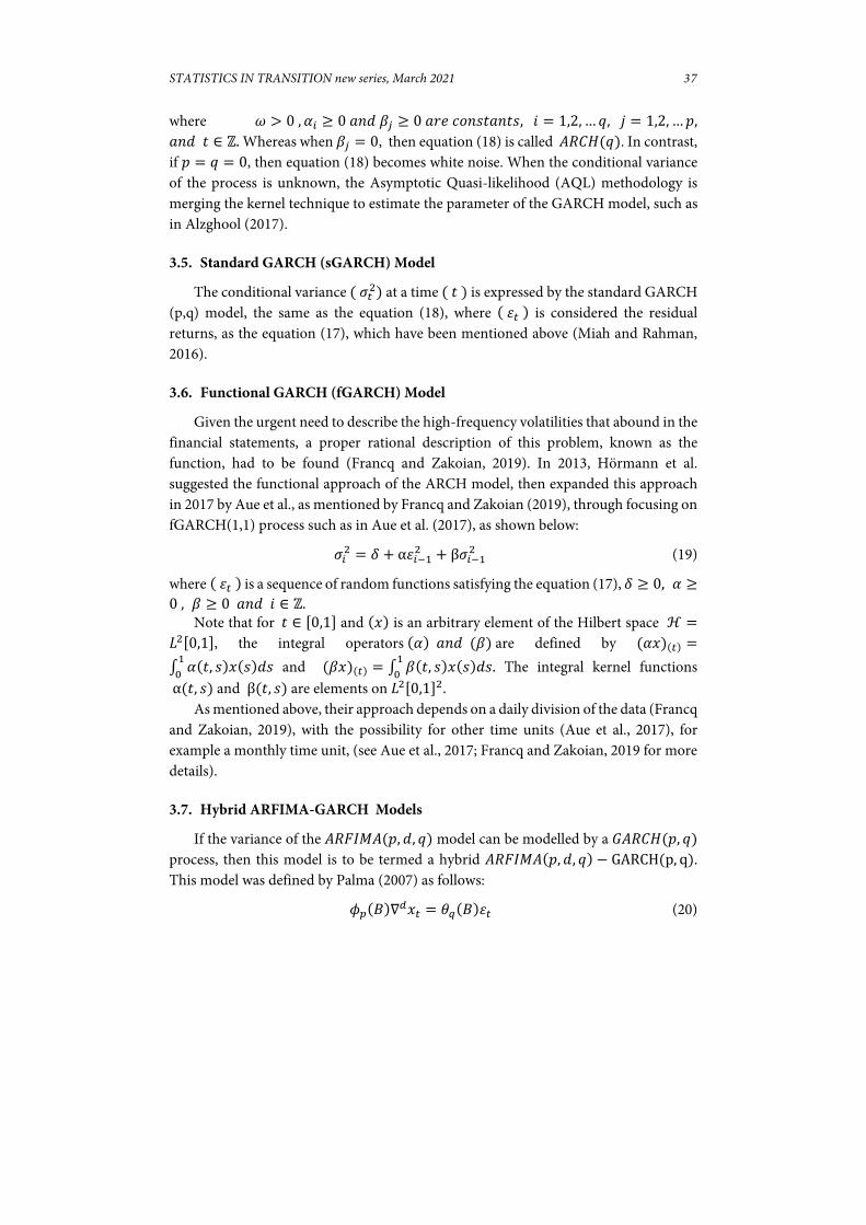
Therefore, this series was studied in terms of having a long memory feature, through graphing and necessary statistical methods. The graph of the Autocorrelation Function (ACF) for time series data in Figure 2 shows a slow decrease.

Figure 2. ACF plot for 𝑋

This gives a preliminary conclusion that there is a long memory, this is confirmed by Table 1 through several statistical methods.

Table 1. Long Memory Tests

R/S Analysis

Aggregated Variance Method

Higuchi Method

H = 0.8531864 H = 0.7910981 H = 0.9578515

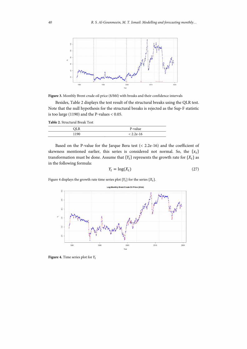
The above table shows the results of three tests to check for the presence of long memory. It is noted that all values of (H) are greater than 0.5, which gives a firm conclusion to the existence of the long memory of the price for Brent crude oil data. Furthermore, the structural breaks are visible in the dataset series. Where, there exists four breaks for Brent are displayed in Figure 3 with the first, second, third, and last break captured in 1986, 1999, 2005, and 2013 respectively.


Figure 3. Monthly Brent crude oil price ($/bbl) with breaks and their confidence intervals

Besides, Table 2 displays the test result of the structural breaks using the QLR test. Note that the null hypothesis for the structural breaks is rejected as the Sup-F statistic is too large (1190) and the P-values < 0.05.

Table 2. Structural Break Test

QLR P-value 1190 < 2.2e-16

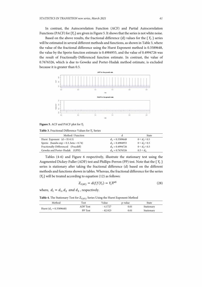
Based on the P-value for the Jarque Bera test (< 2.2e-16) and the coefficient of

skewness mentioned earlier, this series is considered not normal. So, the 𝑥 transformation must be done. Assume that 𝑌 represents the growth rate for 𝑋 as in the following formula:

𝑌 log 𝑋 (27)

Figure 4 displays the growth rate time series plot 𝑌 for the series 𝑋 .

Figure 4. Time series plot for 𝑌


41

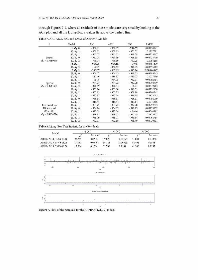
In contrast, the Autocorrelation Function (ACF) and Partial Autocorrelation Functions (PACF) for 𝑌 are given in Figure 5. It shows that the series is not white noise.

Based on the above results, the fractional difference d values for the 𝑌 series will be estimated in several different methods and functions, as shown in Table 3, where the value of the fractional difference using the Hurst Exponent method is 0.3589648, the value by the Sperio function estimate is 0.4984955, and the value of 0.4994726 was the result of Fractionally-Differenced function estimate. In contrast, the value of 0.7676326, which is due to Geweke and Porter-Hudak method estimate, is excluded because it is greater than 0.5.

Figure 5. ACF and PACF plot for 𝑌

Table 3. Fractional Difference Values for 𝑌 Series

Tables (4-6) and Figure 6 respectively, illustrate the stationary test using the Augmented Dickey-Fuller (ADF) test and Phillips-Perron (PP) test. Note that the 𝑌 series is stationary after taking the fractional difference (d) based on the different methods and functions shown in tables. Whereas, the fractional difference for the series {𝑌 will be treated according to equation (12) as follows:

𝑍 𝑑𝑖𝑓𝑓 𝑌 𝑌 ∇ (28)

where, 𝑑 𝑑 , 𝑑 𝑎𝑛𝑑 𝑑 , respectively.

Table 4. The Stationary Test for 𝑍 Series Using the Hurst Exponent Method

Method / Function d State Hurst Exponent (d = H-0.5) 𝑑 = 0.3589648 0 < 𝑑 < 0.5 Sperio (bandw.exp = 0.3, beta = 0.74) 𝑑 = 0.4984955 0 < 𝑑 < 0.5 Fractionally-Differenced (Fracdiff) 𝑑 = 0.4994726 0 < 𝑑 < 0.5 Geweke and Porter-Hudak (GPH) 𝑑 = 0.7676326 0.5 < 𝑑

Method Test Value p-value State

Hurst (𝑑 = 0.3589648) ADF Test - 4.1727 0.01 Stationary

PP Test - 82.923 0.01 Stationary


Table 5. The Stationary Test for 𝑍 Series Using Sperio Function

Table 6. The Stationary Test for 𝑍 Series Using Fractionally-Differenced Function

According to equations 23-26 above, a qualifying model is one that has the lowest value for AIC, AICc, BIC and RMSE. As a result of Table 7, ARFIMA(1,0.3589648,0) model, ARFIMA(2,0.3589648,1) model and ARFIMA(2,0.3589648,2) model have the lowest values for these criteria. Also, it is noted that these models are within the Hurst Exponent estimate, which has the lowest value for the fractional difference estimate d . As a result, the three models will be taken and compared to choose the best among them by moving to the next step of testing the residuals (see Al-Gounmeein and Ismail, 2020). While in this step, residuals testing is a necessary step to examine any model through several methods, including the graph for the ACF and the P-value for the Ljung-Box residuals test, because these methods are important measures to consider correlations of residuals (Montgomery et al., 2015).

Figure 6. Time series plot for 𝑍 using the fractional difference values, respectively

By looking at Table 8, the three models do not have the property of the unit root for the residuals, using the P-value for the Ljung-Box test statistics at Lag(12), Lag(24) and Lag(36). We note that the P-value for the residuals of the third model is larger than the first and the second. In contrast, that model has the smallest Chi-Square statistic 𝜒 at the same different Lags. This is one of the indicators that gives the conclusion

that the ARFIMA 2, 0.3589648 ,2 model is the best. Furthermore, it is observed that

Function Test Value p-value State

Sperio (𝑑 = 0.4984955) ADF Test - 5.1927 0.01 Stationary

PP Test - 151.34 0.01 Stationary

Function Test Value p-value State Fractionally-Differenced (Fracdiff) (𝑑 = 0.4994726)

ADF Test - 5.2001 0.01 Stationary PP Test - 151.89 0.01 Stationary


43

through Figures 7-9, where all residuals of these models are very small by looking at the ACF plot and all the Ljung-Box P-values lie above the dashed line.

Table 7. AIC, AICc, BIC, and RMSE of ARFIMA Models

Table 8. Ljung-Box Test Statistic for the Residuals

Figure 7. Plots of the residuals for the ARFIMA 1, 𝑑 , 0 model

d Model AIC AICc BIC RMSE

Hurst 𝑑 = 0.3589648

(1, 𝒅𝟏 ,0) - 962.91 - 962.89 - 954.59 0.08730141 (0, 𝑑 ,1) - 639.85 - 639.83 - 631.52 0.1227511 (1, 𝑑 ,1) - 961.07 - 961.02 - 948.58 0.08728667 (2, 𝑑 ,0) - 961.04 - 960.99 - 948.55 0.08728949 (0, 𝑑 ,2) - 769.74 - 769.69 - 757.25 0.1068218 (2, 𝒅𝟏 ,1) - 966.25 - 966.16 - 949.6 0.08661429 (1, 𝑑 ,2) - 962.7 - 962.62 - 946.05 0.08695112 (2, 𝒅𝟏 ,2) - 966.07 - 965.95 - 945.26 0.08644647

Sperio 𝑑 = 0.4984955

(1, 𝑑 ,0) - 956.67 - 956.65 - 948.35 0.08793743 (0, 𝑑 ,1) - 818.6 - 818.57 - 810.27 0.1017299 (1, 𝑑 ,1) - 954.8 - 954.75 - 942.31 0.08792554 (2, 𝑑 ,0) - 954.77 - 954.72 - 942.28 0.08792809 (0, 𝑑 ,2) - 876.59 - 876.54 - 864.1 0.09549913 (2, 𝑑 ,1) - 959.16 - 959.08 - 942.51 0.08732158 (1, 𝑑 ,2) - 955.83 - 955.75 - 939.18 0.08764342 (2, 𝑑 ,2) - 957.37 - 957.24 - 936.55 0.0873032

Fractionally – Differenced (Fracdiff)

𝑑 = 0.4994726

(1, 𝑑 ,0) - 956.64 - 956.61 - 948.31 0.08794099 (0, 𝑑 ,1) - 819.47 - 819.44 - 811.14 0.1016366 (1, 𝑑 ,1) - 954.77 - 954.72 - 942.28 0.08792893 (2, 𝑑 ,0) - 954.74 - 954.69 - 942.25 0.08793152 (0, 𝑑 ,2) - 877.09 - 877.04 - 864.6 0.09544912 (2, 𝑑 ,1) - 959.11 - 959.02 - 942.45 0.0873277 (1, 𝑑 ,2) - 955.79 - 955.71 - 939.14 0.08764758 (2, 𝑑 ,2) - 957.31 - 957.18 - 936.49 0.08730851

Model Lag (12) Lag (24) Lag (36)

𝜒 P-value 𝜒 P-value 𝜒 P-value ARFIMA(1,0.3589648,0) 23.247 0.0257 39.895 0.02195 51.031 0.04968 ARFIMA(2,0.3589648,1) 19.037 0.08763 35.148 0.06623 44.401 0.1588 ARFIMA(2,0.3589648,2) 17.594 0.1286 32.708 0.1104 41.946 0.2287




While that the P-value for the Jarque Bera test for the residual’s models ARFIMA 1, 𝑑 ,0 , ARFIMA 2, 𝑑 ,1 and ARFIMA 2, 𝑑 ,2 is 2.2𝑒 . As for the P-value for the Shapiro-Wilk normality test for these models’ residuals are 1.585𝑒 , 1.919𝑒 , and 1.686𝑒 , respectively. As a result, these models’ residuals are not normally distributed.

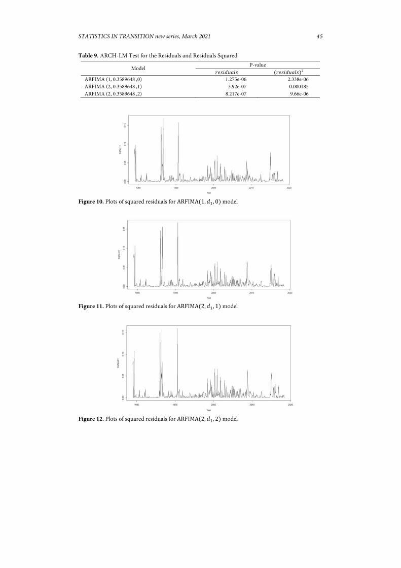
On the other hand, when examining the residuals, it was observed that there exists Heteroscedasticity and ARCH effect using the ARCH Lagrange Multiplies (ARCH-LM) test for the residuals and residuals squared as shown in the P-value for the three models of ARFIMA in Table 9. Where all P-values for residuals and residuals squared in the ARCH-LM test less than 0.05. Therefore, we reject 𝐻 . This means there exists an ARCH effect. As well as when returning to Table 8 using the Ljung-Box test statistic. Certainly, illustrated by showing the Heteroskedasticity for the squared residuals in Figures 10-12 for these models, respectively.


45

Table 9. ARCH-LM Test for the Residuals and Residuals Squared

Figure 10. Plots of squared residuals for ARFIMA 1, 𝑑 , 0 model



Model P-value 𝑟𝑒𝑠𝑖𝑑𝑢𝑎𝑙𝑠 𝑟𝑒𝑠𝑖𝑑𝑢𝑎𝑙𝑠

ARFIMA (1, 0.3589648 ,0) 1.275e-06 2.338e-06 ARFIMA (2, 0.3589648 ,1) 3.92e-07 0.000185 ARFIMA (2, 0.3589648 ,2) 8.217e-07 9.66e-06


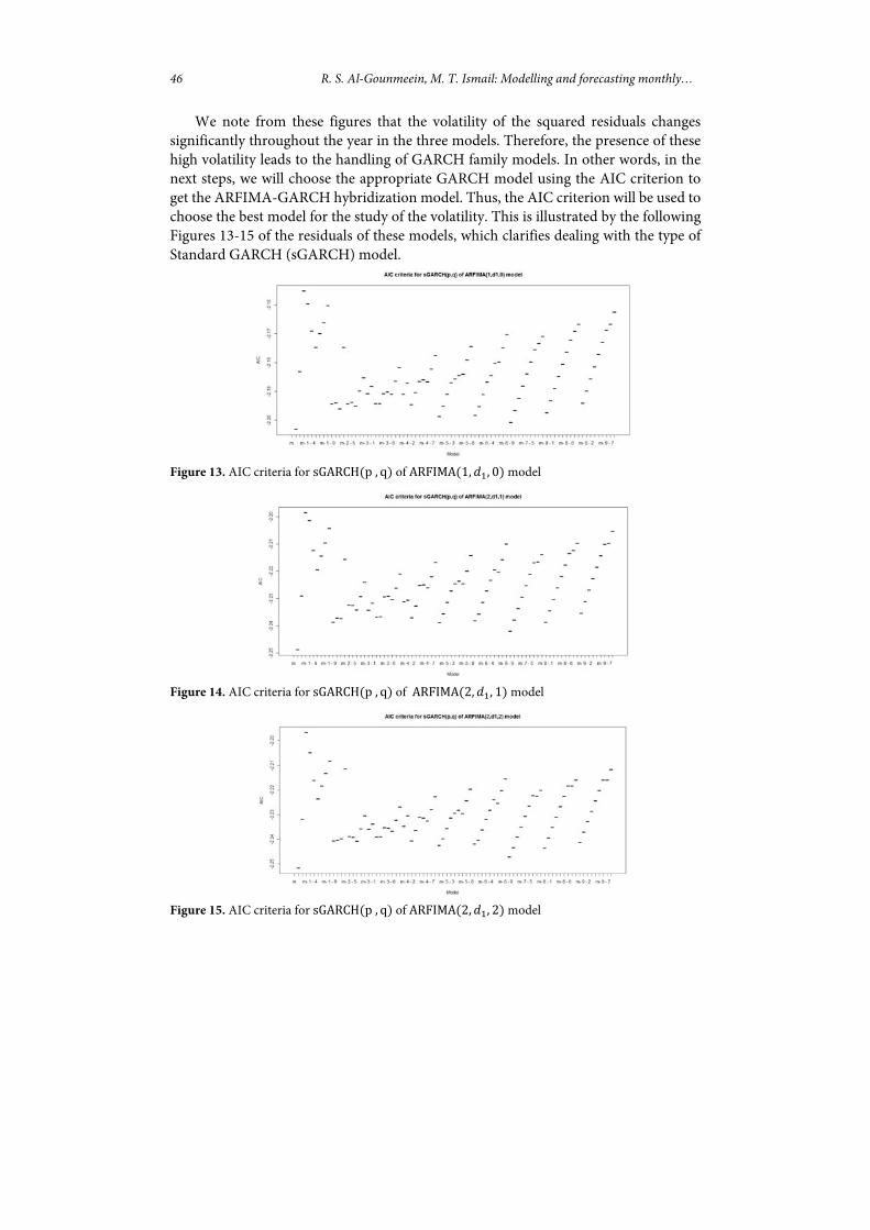
We note from these figures that the volatility of the squared residuals changes significantly throughout the year in the three models. Therefore, the presence of these high volatility leads to the handling of GARCH family models. In other words, in the next steps, we will choose the appropriate GARCH model using the AIC criterion to get the ARFIMA-GARCH hybridization model. Thus, the AIC criterion will be used to choose the best model for the study of the volatility. This is illustrated by the following Figures 13-15 of the residuals of these models, which clarifies dealing with the type of Standard GARCH (sGARCH) model.

Figure 13. AIC criteria for sGARCH p , q of ARFIMA 1, 𝑑 , 0 model




47

The graphical test of AIC criteria above (Figures 13-15) indicates that the best volatility model for these three models is sGARCH(1,1). Also, based on the smallest value of this criterion for sGARCH 1,1 of ARFIMA 1, 𝑑 ,0 model, ARFIMA 2, 𝑑 ,1 model and ARFIMA 2, 𝑑 ,2 model is (-2.203081, -2.248740 and -2.251659), respectively.

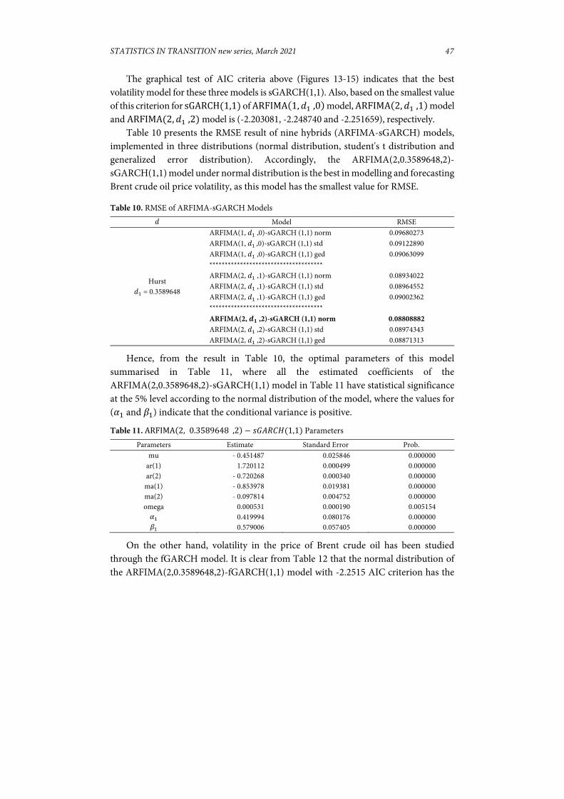
Table 10 presents the RMSE result of nine hybrids (ARFIMA-sGARCH) models, implemented in three distributions (normal distribution, student's t distribution and generalized error distribution). Accordingly, the ARFIMA(2,0.3589648,2)-sGARCH(1,1) model under normal distribution is the best in modelling and forecasting Brent crude oil price volatility, as this model has the smallest value for RMSE.

Table 10. RMSE of ARFIMA-sGARCH Models 𝑑 Model RMSE

Hurst 𝑑 = 0.3589648

ARFIMA(1, 𝑑 ,0)-sGARCH (1,1) norm 0.09680273 ARFIMA(1, 𝑑 ,0)-sGARCH (1,1) std 0.09122890 ARFIMA(1, 𝑑 ,0)-sGARCH (1,1) ged 0.09063099 ************************************* ARFIMA(2, 𝑑 ,1)-sGARCH (1,1) norm 0.08934022 ARFIMA(2, 𝑑 ,1)-sGARCH (1,1) std 0.08964552 ARFIMA(2, 𝑑 ,1)-sGARCH (1,1) ged 0.09002362 ************************************* ARFIMA(2, 𝒅𝟏 ,2)-sGARCH (1,1) norm 0.08808882 ARFIMA(2, 𝑑 ,2)-sGARCH (1,1) std 0.08974343 ARFIMA(2, 𝑑 ,2)-sGARCH (1,1) ged 0.08871313

Hence, from the result in Table 10, the optimal parameters of this model summarised in Table 11, where all the estimated coefficients of the ARFIMA(2,0.3589648,2)-sGARCH(1,1) model in Table 11 have statistical significance at the 5% level according to the normal distribution of the model, where the values for (𝛼 and 𝛽 ) indicate that the conditional variance is positive.

Table 11. ARFIMA 2, 0.3589648 ,2 𝑠𝐺𝐴𝑅𝐶𝐻 1,1 Parameters Parameters Estimate Standard Error Prob.

mu - 0.451487 0.025846 0.000000 ar(1) 1.720112 0.000499 0.000000 ar(2) - 0.720268 0.000340 0.000000 ma(1) - 0.853978 0.019381 0.000000 ma(2) - 0.097814 0.004752 0.000000 omega 0.000531 0.000190 0.005154

𝛼 0.419994 0.080176 0.000000 𝛽 0.579006 0.057405 0.000000

On the other hand, volatility in the price of Brent crude oil has been studied through the fGARCH model. It is clear from Table 12 that the normal distribution of the ARFIMA(2,0.3589648,2)-fGARCH(1,1) model with -2.2515 AIC criterion has the


smallest RMSE. Also, the same hybridization model was obtained in Table 10 with a different type of GARCH family. This is shown in Table 12.

By looking at Table 13, which shows the optimal parameters for this model, it has the same statistical significance as the model of ARFIMA(2,0.3589648,2)-sGARCH(1,1) in Table 11. In other words, the significance of alpha and beta values in the two models indicates that the price’s volatilities in the past period affect the current price’s volatilities.

As a result of this study, it was found that ARFIMA(2,0.3589648,2)-sGARCH(1,1) model and ARFIMA(2,0.3589648,2)-fGARCH(1,1) model under normal distribution are equal in the value of RMSE. Thus, these two models will be taken and moved to the next step, the model validation phase preceding the prediction phase.

Table 12. RMSE of ARFIMA-fGARCH Models

𝑑 Model RMSE

Hurst 𝑑 = 0.3589648

ARFIMA(1, 𝑑 ,0)-fGARCH (1,1) norm 0.09681124 ARFIMA(1, 𝑑 ,0)-fGARCH (1,1) std 0.09122962 ARFIMA(1, 𝑑 ,0)-fGARCH (1,1) ged 0.09063172 *************************************** ARFIMA(2, 𝑑 ,1)- fGARCH (1,1) norm 0.08934022 ARFIMA(2, 𝑑 ,1)- fGARCH (1,1) std 0.08964552 ARFIMA(2, 𝑑 ,1)- fGARCH (1,1) ged 0.09002547 *************************************** ARFIMA(2, 𝒅𝟏 ,2)-fGARCH (1,1) norm 0.08808882 ARFIMA(2, 𝑑 ,2)- fGARCH (1,1) std 0.08974902 ARFIMA(2, 𝑑 ,2)- fGARCH (1,1) ged 0.08871313

Table 13. ARFIMA 2, 0.3589648 ,2 𝑓𝐺𝐴𝑅𝐶𝐻 1,1 Parameters

Parameters Estimate Standard Error Prob.

mu - 0.451487 0.025847 0.000000 ar(1) 1.720112 0.000499 0.000000 ar(2) - 0.720268 0.000340 0.000000 ma(1) - 0.853977 0.019381 0.000000 ma(2) - 0.097815 0.004752 0.000000 omega 0.000531 0.000190 0.005154

𝛼 0.419992 0.080176 0.000000 𝛽 0.579007 0.057405 0.000000

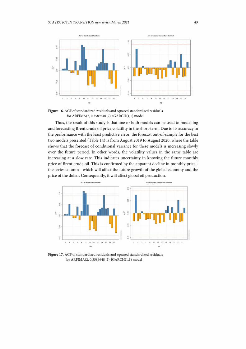
Based on the above outcomes of the identification, estimation and diagnosis stages, the final validation of the two hybridization models is necessary by testing the residuals. By using the P-value for the Ljung-Box statistical test, we note that the P-value for the residuals of two hybridization models equals 0.993 > 0.05. It means that these two models have the property of the unit root or independent residuals. On the other hand, this can be confirmed by the figures for ACF of standardized residuals and ACF of squared standardized residuals shown in Figures 16-17 respectively (see Iqelan, 2015).


49

Figure 16. ACF of standardized residuals and squared standardized residuals

for ARFIMA(2, 0.3589648 ,2)-sGARCH(1,1) model

Thus, the result of this study is that one or both models can be used to modelling and forecasting Brent crude oil price volatility in the short-term. Due to its accuracy in the performance with the least predictive error, the forecast out-of-sample for the best two models presented (Table 14) is from August 2019 to August 2020, where the table shows that the forecast of conditional variance for these models is increasing slowly over the future period. In other words, the volatility values in the same table are increasing at a slow rate. This indicates uncertainty in knowing the future monthly price of Brent crude oil. This is confirmed by the apparent decline in monthly price - the series column - which will affect the future growth of the global economy and the price of the dollar. Consequently, it will affect global oil production.

Figure 17. ACF of standardized residuals and squared standardized residuals

for ARFIMA(2, 0.3589648 ,2)-fGARCH(1,1) model


Table 14. Forecast Out-of-Sample for ARFIMA 2, 0.3589648 ,2 𝑠𝐺𝐴𝑅𝐶𝐻 1,1 Model and ARFIMA 2, 0.3589648 ,2 𝑓𝐺𝐴𝑅𝐶𝐻 1,1 Model

The result of this study calls for the development of the best strategic plans and

vision for the future by economists, investors, and analysts to take advantage of the uncertainty in Brent crude oil prices in the future. Also, it is possible to conduct similar studies on Brent crude oil price when the case study for the fractional difference value is greater than 0.5 for ARFIMA models or the study of ARFIMA models in terms of seasonal presence.

5. Conclusion

This paper is designed to determine the modelling and forecasting of monthly Brent crude oil price and its volatility. Also, it extended the works from the previous literature by examining long memory and volatilities in the dataset simultaneously, by using the comparison of the ARFIMA-sGARCH models versus the ARFIMA-fGARCH models. It was noted that the ARFIMA(2,0.3589648,2)-sGARCH(1,1) model and ARFIMA(2,0.3589648,2)-fGARCH(1,1) model under normal distribution with RMSE, which equals (0.08808882) are the best for these data, where these models outperform other several models in modelling and forecasting the volatility. The forecasts for these models indicated a decline in the price in the short-term. On the other hand, the Hurst Exponent method outperformed constructing an appropriate hybridization model to predict. Finally, we obtained distinct results for our study that distinguish it from other previous studies, namely: two-hybrid models of long memory phenomenon (ARFIMA) were obtained with two members of the GARCH family (sGARCH and fGARCH) having the same accuracy in RMSE value. Also, the best model does not have the smallest AIC value, which gives the conclusion that taking a single value for the AIC

Year

Month

ARFIMA 2, 𝑑 ,2 𝑠𝐺𝐴𝑅𝐶𝐻 1,1 ARFIMA 2, 𝑑 ,2 𝑓𝐺𝐴𝑅𝐶𝐻 1,1 Series Sigma Series Sigma

2019

Aug Sep Oct Nov Dec

64.436 63.810 63.311 62.709 62.214

4.4553 4.4756 4.4959 4.5160 4.5360

64.436 63.810 63.311 62.709 62.214

4.4553 4.4756 4.4959 4.5160 4.5360

2020

Jan Feb Mar Apr May Jun Jul Aug

61.634 61.144 60.584 60.100 59.558 59.081 58.557 58.088

4.5559 4.5758 4.5955 4.6150 4.6345 4.6539 4.6732 4.6924

61.634 61.144 60.584 60.100 59.559 59.081 58.557 58.088

4.5559 4.5757 4.5954 4.6150 4.6345 4.6539 4.6732 4.6924


51

criterion is not sufficient to choose the best model among the models. Therefore, it is proposed to consider taking the two smallest values in accuracy criteria such as AIC and not just the smallest value, and this is what this study showed.

References

AAMIR, M., SHABRI, A. B., (2015). Modelling and Forecasting Monthly Crude Oil Prices of Pakistan: A Comparative Study of ARIMA, GARCH and ARIMA-GARCH Models. Sci.Int. (Lahore), 27(3), pp. 2365−2371.

AKRON, N., ISMAIL, Z., (2017). A hybrid GA-FEEMD for forecasting crude oil prices. Indian Journal of Science and Technology, 10(31), pp. 1−6.

AKTER, N., NOBI, A., (2018). Investigation of the Financial Stability of S&P 500 Using Realized Volatility and Stock Returns Distribution. Journal of Risk Financial Management, 11(22), pp. 1−10.

AL-GOUNMEEIN, R. S., ISMAIL, M. T., (2020). Forecasting the Exchange Rate of the Jordanian Dinar versus the US Dollar Using a Box-Jenkins Seasonal ARIMA Model. International Journal of Mathematics and Computer Science, 15(1), pp. 27−40.

AMBACH, D., AMBACH, O., (2018). Forecasting the oil price with a periodic regression ARFIMA-GARCH process. IEEE Second International Conference on Data Stream Mining & Processing, Lviv, Ukraine, pp. 212−217.

ALZGHOOL, R., (2017). Parameters estimation for GARCH (p,q) model: QL and AQL approaches. Electronic Journal of Applied Statistical Analysis, 10(1), pp.180−193.

AUE, A., HORVATH, L. and PELLATT, D. F., (2017). Functional generalized autoregressive conditional heteroskedasticity. Journal of Time Series Analysis, 38(1), pp. 3−21.

BAHAR, A., NOH, N. M. and ZAINUDDIN, Z. M., (2017). Forecasting model for crude oil price with structural break. Malaysian Journal of Fundamental and Applied Sciences, pp. 421−424.

BERAN, J., (1994). Statistics for Long Memory Processes, Chapman and Hall, p. 315.

BHARDWAJ, G., SWANSON, N. R., (2006). An empirical investigation of the usefulness of ARFIMA models for predicting macroeconomic and financial time series. Journal of Econometrics 131, pp. 539−578.


BOUTAHAR, M., MARIMOUTOU, V. and NOUIRA, L., (2007). Estimation Methods of the Long Memory Parameter: Monte Carlo Analysis and Application. Journal of Applied Statistics, 34(3), pp. 261−301.

BOX, G. E. P., JENKINS, G. M. and REINSEL, G. C., (2008). Time series analysis forecasting and control, Fourth Edition, Wiley & Sons, Inc, p. 746.

CRYER, J. D., CHAN, K., (2008). Time Series Analysis With Application in R, Second Edition, Springer, p. 491.

DIEBOLD, F. X., INOUE, A., (2001). Long Memory and Regime Switching. Journal of Econometrics, 105, pp. 131−159.

FAZELABDOLABADI, B., (2019). A hybrid Bayesian-network proposition for forecasting the crude oil price. Financial Innovation, 5(30), pp. 1−21.

FRANCQ, C., ZAKOIAN, J. M., (2019). GARCH Models: Structure, Statistical Inference and Financial Applications, Second Edition, John Wiley & Sons Ltd, p. 487.

GRANGER, C. W. J., HYUNG, N., (2004). Occasional structural breaks and long memory with an application to the S&P 500 absolute stock returns. Journal of Empirical Finance, 11, pp. 399−421.

HE, X. J., (2018). Crude Oil Prices Forecasting: Time Series vs. SVR Models. Journal of International Technology and Information Management, 27(2), pp. 25−42.

HOSKING, J. R. M., (1981). Fractional differencing. Biometrika, 86(1), pp. 165−176.

IQELAN, B. M., (2015). Time Series Modeling of Monthly Temperature Data of Jerusalem / Palestine. MATEMATIKA, 31(2), pp. 159−176.

ISMAIL, M. T., AWAJAN, A. M., (2017). A new hybrid approach EMD-EXP for short-term forecasting of daily stock market time series data. Electronic Journal of Applied Statistical Analysis, 10(2), pp. 307−327.

JIBRIN, S. A., MUSA, Y., ZUBAIR, U. A. and SAIDU, A. S., (2015). ARFIMA Modelling and Investigation of Structural Break(s) in West Texas Intermediate and Brent Series, CBN Journal of Applied Statistics, 6(2), pp. 59−79.

KANG, S. H., YOON, S., (2013). Modeling and forecasting the volatility of petroleum futures prices. Energy Economics, 36, pp. 354−362.

KARIA, A. A., BUJANG, I. and AHMAD, I., (2013). Fractionally integrated ARMA for crude palm oil prices prediction: case of potentially over difference. Journal of Applied Statistics, 40(12), pp. 2735−2748.


53

LEE, C. Y., HUH, S. Y., (2017). Forecasting Long-Term Crude Oil Prices Using a Bayesian Model with Informative Priors. Sustainability. 9, 190, DOI: 10.3390/su9020190.

LO, A. W., (1991). Long-term memory in stock market prices. Econometrica, 59(5), pp. 1279−1313.

MANDELBROT, B., (1972). Statistical Methodology for Nonperiodic Cycles: From the Covariance to R/S Analysis. Annals of Economic and Social Measurement, 1(3), pp. 259−290.

MANERA, M., MCALEER, M. and GRASSO, M., (2004). Modelling dynamic conditional correlations in the volatility of spot and forward oil price returns, 2nd International Congress on Environmental Modelling and Software - Osnabrück, Germany, 183, pp. 1−6.

MIAH, M., RAHMAN, A., (2016). Modelling Volatility of Daily Stock Returns: Is GARCH(1,1) Enough?. American Scientific Research Journal for Engineering, Technology, and Sciences (ASRJETS), 18(1), pp. 29−39.

MONTGOMERY, D. C., JENNINGS, C. L. and KULAHCI, M., (2015). Introduction To Time Series Analysis And Forecasting, Second Edition, Wiley & Sons, Inc, p. 643.

MOSTAFAEI, H., SAKHABAKHSH, L., (2012). Using SARFIMA Model to Study and Predict the Iran’s Oil Supply. International Journal of Energy Economics and Policy, 2(1), pp. 41−49.

NYANGARIKA, A., MIKHAYLOV, A. and RICHTER, U. H., (2019). Oil Price Factors: Forecasting on the Base of Modified Auto-regressive Integrated Moving Average Model. International Journal of Energy Economics and Policy, 9(1), pp. 149−159.

OHANISSIAN, A., RUSSELL, J. R. and TSAY, R. S., (2008). True or Spurious Long Memory? A New Test. Journal of Business & Economic Statistics, 26(2), pp. 161−175.

OLATAYO, T. O., ADEDOTUN, A. F., (2014). On the Test and Estimation of Fractional Parameter in ARFIMA Model: Bootstrap Approach. Applied Mathematical Sciences, 8(96), pp.4783−4792.

PALMA, W., (2007). Long-Memory Time Series: Theory and Methods, John Wiley & Sons, Inc, p. 285.


PRETIS, F., SCHNEIDER, L., SMERDON, J. E. and HENDRY, D. F., (2016). Detecting volcanic eruptions in temperature reconstructions by designed break-indicator saturation. Journal of Economic Surveys, 30(3), pp. 403−429.

RAMZAN, S., RAMZAN, S. and ZAHID, F. M., (2012). Modeling and Forecasting Exchange Rate Dynamics In Pakistan Using ARCH Family of Models. Electronic Journal of Applied Statistical Analysis, 5(1), pp. 15−29.

REISEN, V. A., (1994). Estimation of the Fractional Difference Parameter in the ARIMA(p,d,q) Model Using the Smoothed Periodogram. Journal of Time Series Analysis, 15(3), pp. 335−350.

SEHGAL, N., PANDEY, K. K., (2015). Artificial intelligence methods for oil price forecasting: a review and evaluation, Springer-Verlag Berlin Heidelberg, DOI: 10.1007/s12667-015-0151-y.

TELBANY, S., SOUS, M., (2016). Using ARFIMA Models in Forecasting Indicator of the Food and Agriculture Organization. IUGJEBS, 24(1), pp. 168−187.

TENDAI, M., CHIKOBVU, D., (2017). Modelling international tourist arrivals and volatility to the Victoria Falls Rainforest, Zimbabwe: Application of the GARCH family of models. African Journal of Hospitality, Tourism and Leisure, 6(4), pp. 1−16.

YIN, X., PENG, J. and TANG, T., (2018). Improving the Forecasting Accuracy of Crude Oil Prices. Sustainability. 10, 454, DOI: 10.3390/su10020454.

YU, L., WANG, S. and LAI, K. K., (2008). Forecasting crude oil price with an EMD-based neural network ensemble learning paradigm. Energy Economics, 30, pp. 2623−2635.

YU, L., ZHANG, X. and WANG, S., (2017). Assessing Potentiality of Support Vector Machine Method in Crude Oil Price Forecasting. EURASIA Journal of Mathematics, Science and Technology Education, 13(12), pp. 7893-7904.

Modelling and forecasting monthly Brent crude oil prices ...

Documents

Transcript of Modelling and forecasting monthly Brent crude oil prices ...