Modelling and Control of the UAV Sky-Sailor Mattio Master Project Summer 2006 Modelling and Control...
88
Autonomous Systems Laboratory, ASL Master project Modelling and Control of the UAV Sky-Sailor Professor: Roland Siegwart Andrea Mattio Assistants: André Noth Samir Bouabdallah Sébastien Gros
Transcript of Modelling and Control of the UAV Sky-Sailor Mattio Master Project Summer 2006 Modelling and Control...

Autonomous Systems Laboratory, ASL
Master project
Modelling and Control of the UAV Sky-Sailor
Professor: Roland Siegwart Andrea Mattio Assistants: André Noth Samir Bouabdallah Sébastien Gros

INDEX
1 Introduction ______________________________________ 5
2 Sky-Sailor dynamic model __________________________ 7 2.1 Assumptions of the model ___________________________________________________ 7 2.2 Modelling with Euler-Lagrange method _______________________________________ 8 2.3 Reference frames fixation ___________________________________________________ 8 2.4 6DoF fixed mass rigid body model ___________________________________________ 10 2.5 Aerodynamic forces of an airfoil_____________________________________________ 12 2.6 Non conservative forces model ______________________________________________ 14 2.7 Airfoil coefficient analysis __________________________________________________ 15
2.7.1 Induced Drag ___________________________________________________________________17 2.8 Modeling group Motor-Gearbox-Propeller ____________________________________ 18 2.9 Simulink simulator ________________________________________________________ 21
2.9.1 Notes on the simulator____________________________________________________________22
3 Control model definition ___________________________ 23 3.1 Lift, Drag and Moment Coefficient analysis ___________________________________ 23
3.1.1 Lift and Moment coefficient interpolation_____________________________________________23 3.1.2 Drag coefficient interpolation ______________________________________________________25
3.2 New sequence of Tait-Bryant angles__________________________________________ 27 3.2.1 Relationship between the different sequences __________________________________________27
3.3 Differential use of the ailerons_______________________________________________ 28
4 Control strategy__________________________________ 29 4.1 Choice of a method for the Low Level Control (LLC) ___________________________ 30 4.2 Choice of a method for the High Level Control (HLC) __________________________ 30
5 Model linearization _______________________________ 31 5.1 Search of a steady-state point _______________________________________________ 31
5.1.1 Steady-state point for a straight flight ________________________________________________31 5.1.2 Steady-state point for a circular flight ________________________________________________36
5.2 Model linearization around the steady-state point ______________________________ 38
6 Low level control: Linear Quadratic Regulator __________ 41
6.1 Linear quadratic control ___________________________________________________ 41 6.2 Solution of Riccati equation_________________________________________________ 41 6.3 Linear Quadratic Regulator for Sky-Sailor____________________________________ 42
6.3.1 Model Reduction ________________________________________________________________42 6.3.2 Analysis of controllability _________________________________________________________44

Andrea Mattio Master Project Summer 2006
Modelling and Control of the UAV Sky-Sailor
3
6.3.3 Choice of Q and R _______________________________________________________________45 6.3.4 LQR with integral action __________________________________________________________46
7 High level control_________________________________ 49 7.1 Heading generator ________________________________________________________ 50
7.1.1 Velocity scheduling controller for a nonholonomic mobile robot [3] ________________________50 7.1.2 From heading to roll set point ______________________________________________________51
8 HLC and LLC fusion: simulation _____________________ 52 8.1 Altitude saturation and commands filter ______________________________________ 52 8.2 Necessity of a HLC ________________________________________________________ 53 8.3 Sky-Sailor behavior in simulation____________________________________________ 54
8.3.1 Without wind disturbs ____________________________________________________________55 8.3.2 With wind disturbs_______________________________________________________________56
9 Embedded system on Sky-Sailor ____________________ 59
9.1 DSPIC __________________________________________________________________ 60 9.2 Sensors__________________________________________________________________ 60
9.2.1 IMU (Inertial Measurement Unit) ___________________________________________________60 9.2.2 Airspeed sensor _________________________________________________________________62 9.2.3 Altimeter ______________________________________________________________________63 9.2.4 Miniature GPS__________________________________________________________________63
10 Control implementation on the DSPIC _______________ 64 10.1 General functional scheme__________________________________________________ 64 10.2 LLC implementation ______________________________________________________ 65 10.3 HLC implementation ______________________________________________________ 67 10.4 Timer organization________________________________________________________ 68
11 Conclusions ___________________________________ 69 11.1 Modeling ________________________________________________________________ 69 11.2 Control__________________________________________________________________ 69
12 Acknowledgments ______________________________ 70
13 Bibliography ___________________________________ 71
14 Annexes ______________________________________ 73 14.1 Least mean squares method ________________________________________________ 73 14.2 Conventions used _________________________________________________________ 74 14.3 Relationship between different Tait-Bryant sequence: details_____________________ 76 14.4 From angular rates to angles derivatives ______________________________________ 77 14.5 LLC behaviour ___________________________________________________________ 77 14.6 Implementation details_____________________________________________________ 80

Andrea Mattio Master Project Summer 2006
Modelling and Control of the UAV Sky-Sailor
4
14.6.1 Numerical Integration with Euler method___________________________________________80 14.6.2 Numerical interpolation ________________________________________________________81 14.6.3 Filter implementation __________________________________________________________82 14.6.4 LLC pseudo code _____________________________________________________________82 14.6.5 HLC pseudo code _____________________________________________________________83
14.7 Fourier Transformation and Power Spectral Density ___________________________ 84 14.8 dsPIC general features_____________________________________________________ 85 14.9 Bus I2C _________________________________________________________________ 87

Andrea Mattio Master Project Summer 2006
Modelling and Control of the UAV Sky-Sailor
5
1 Introduction The Autonomous System Lab of EPFL1 is developing an ultra-lightweight solar autonomous
model airplane called Sky-Sailor with embedded navigation and control system. The main goal
of this project is to jointly undertake research on navigation, control of the plane and also work
on the design of the structure and the energy generation system. The airplane should be capable
of continuous flight over days and nights, which makes it suitable for a wide range of
applications. In the figure is represented the general structure of Sky-Sailor.
Figure 1.1: Sky-Sailor overview
The main objectives of this Master Project are the following:
• Complete and exhaustive modelling of Sky-Sailor to obtain a good simulation model
• Creation of a good control model
• Design of a control able to stabilize the plane and to reject perturbations as wind
• Test and validation of the control in simulation
• Implementation of the control on the real system
• Test and validation of the control on the real system
• The major challenges to overtake are:
• Good aerodynamic knowledge of the structure
• Design of a control at the same robust but able to reduce consumed energy
1 École Polytechnique Fédérale de Lausanne

Andrea Mattio Master Project Summer 2006
Modelling and Control of the UAV Sky-Sailor
6
• Design of a control robust but easy and light to implement
• Saving energy while implementing
A great difficulty working with flying object is the danger and the risk always present during
tests. Losing contact with the plane while flying at 200 meters high is quite dangerous for the
plane but not only. The reliability of the system must be as higher as possible.

Andrea Mattio Master Project Summer 2006
Modelling and Control of the UAV Sky-Sailor
7
2 Sky-Sailor dynamic model Sky-Sailor is a model-scale solar airplane that is intended to achieve continuous flight with the
only energy of the sun. It consists of a glider with a wingspan of 3.2 meters that is motorized by
a DC motor connected to the propeller (a) through a gearbox. The control surfaces are:
Two ailerons (b) on the main wing that act mainly on the roll of the airplane
The V-tail (c) at the rear side composed of two control surfaces that act mainly on the pitch if
they change symmetrically (elevator) and on the yaw if their deviation is not symmetrical
(rudder).
Figure 2.1: Sky-Sailor
2.1 Assumptions of the model
The flying systems are very difficult to model, because of the quantity of dynamic and
aerodynamic effects acting on them; so it’s necessary to make some assumptions in order to find
out a correct but at the same time simplified model of the airplane.
The airplane is considered as a 6DoF fixed mass rigid body on which they are acting the
aerodynamic forces of lift, drag and moment
The centre of mass and the body fixed frame origin are assumed to coincide
The structure is supposed rigid and symmetric (diagonal inertia matrix).
The wind speed in the Earth frame is set to zero so that the relative wind on the body frame is
only due to the airplane speed.
X
Y E
Z
a
b
b c
z
x
y
roll
yaw
pitch
e

Andrea Mattio Master Project Summer 2006
Modelling and Control of the UAV Sky-Sailor
8
2.2 Modelling with Euler-Lagrange method
First one has to model the behavior of a 6DoF fixed mass rigid body moving in the space. To
achieve this target it’s possible to use Euler-Lagrange or Newton-Euler approach. The simpler,
moreover from the point of view of calculation time, is Euler-Lagrange. Anyway it’s useful to
underline that both methods lead to the same final result.
Euler-Lagrange approach uses the concepts of potential and kinetic energies in order to obtain
the final equations.
iii q
LqL
dtd
∂∂
−⎟⎟⎠
⎞⎜⎜⎝
⎛∂∂
=Γ (2.1)
where VTL −= is called the Lagrangian (2.2)
with iq : generalized coordinates
iΓ : generalized forces dues to the non conservative forces
T : total kinetic energy
V : total potential energy
2.3 Reference frames fixation
It’s necessary to fix the reference frames and the conventions about angles, rotations and
positions in the different reference frames. Two different reference frames were used, one fixed
to the airplane (body reference frame) and the other one fixed to the earth (earth reference
frame). From now on we will use the following symbolic convention:
eX : Variable in the body reference frame
EX : Variable in the earth reference frame
The earth-fixed reference frame is considered inertial, a simplification that allows the forces due
to the Earth's motion relative to a star-fixed reference system to be neglected.

Andrea Mattio Master Project Summer 2006
Modelling and Control of the UAV Sky-Sailor
9
Figure 2.2: Earth-fixed and body fixed reference frames
One can define the position of a point in the space with cartesian, cylindrical or spherical
coordinates. Usually the chosen system is the cartesian one which allows to describe a rotation
with Euler angles. It’s useful to underline that many times Euler angles are confused with the
angles of Cardano also named angles of Tait-Bryant in the aerodynamic field.
Euler angles describe the following rotations:
Rotation of ψ around Z : uX ⇒
Rotation of θ around u : zZ ⇒
Rotation of φ around z : xu ⇒
Figure 2.3: Euler angles representation
Tait-Bryant angles describe instead the following rotations:
Rotation of φ around x : (roll angle with πφπ <<− )
Rotation of θ around y : (pitch angle with 22 πφπ <<− )
Rotation of ψ around z : (yaw angle with πψπ <<− )

Andrea Mattio Master Project Summer 2006
Modelling and Control of the UAV Sky-Sailor
10
Figure 2.4: Tait-Bryant angles representation
The following rotation matrixes can be written:
( ) ( ) ( )⎥⎥⎥
⎦
⎤
⎢⎢⎢
⎣
⎡ −=
⎥⎥⎥
⎦
⎤
⎢⎢⎢
⎣
⎡
−=
⎥⎥⎥
⎦
⎤
⎢⎢⎢
⎣
⎡−=
1000cossin0sincos
,cos0sin
010sin0cos
,cossin0sincos0001
, γγγγ
γββ
βββ
ααααα zRyRxR
Multiplying the three matrixes it’s possible to obtain the total rotation matrix:
( ) ( ) ( ) ( )φθψψθφ ,,,,, xRyRzRR ⋅⋅=
( )⎥⎥⎥
⎦
⎤
⎢⎢⎢
⎣
⎡−⋅
⎥⎥⎥
⎦
⎤
⎢⎢⎢
⎣
⎡
−⋅
⎥⎥⎥
⎦
⎤
⎢⎢⎢
⎣
⎡ −=
φφφφ
θθ
θθψψψψ
ψθφcossin0sincos0001
cos0sin010
sin0cos
1000cossin0sincos
,,R
( )⎥⎥⎥
⎦
⎤
⎢⎢⎢
⎣
⎡
−−++−
=φθφθθ
ψφφθψφψθψθψφψφθψφψφθψθψ
ψθφcoscossincossin
cossincossinsincoscossinsinsincossinsinsincossincoscossinsinsincoscoscos
,,R (2.3)
Tait-Bryant angles were chosen in the present case because they are the most used in the
aerodynamic field and they reflect well the various rotations acting on the airplane, as the MTX
IMU sensor uses the same convention.
2.4 6DoF fixed mass rigid body model
The first step consists of modeling the behavior of six degrees of freedom fixed mass rigid body
moving in the space referred to an earth-fixed reference frame.
To develop these equations one uses Euler-Lagrange formalism:

Andrea Mattio Master Project Summer 2006
Modelling and Control of the UAV Sky-Sailor
11
iii q
LqL
dtd
∂∂
−⎟⎟⎠
⎞⎜⎜⎝
⎛∂∂
=Γ
VTL −=
with iq : generalized coordinates
iΓ : generalized forces dues to the non conservative forces
T : total kinetic energy
V : total potential energy
The kinetic energy due to the translation is immediately:
222
21
21
21 ZMYMXME tran
kin ++= (2.4)
As stated it in the hypotheses, one assumes that the inertia matrix is diagonal and thus, that the
inertia products are equal to zero. The kinetic energy due to the rotation is:
222
21
21
21
zzzyyyxxxrotkin IIIE ωωω ++= (2.5)
Where zyx ωωω ,, are the rotational speeds in the body fixed reference frame that can be
expressed as a function of the roll, pitch and yaw ( )ψθφ ,, and of the relative rates ( )ψθφ ,, . It’s
useful to point out that the time variation of Tait-Bryant angles ( )ψθφ ,, is a discontinuous
function. Thus, it is different from body angular rates ( , , )p q r which are physically measured
with gyroscopes for instance. In the aerodynamic field usually:
⎟⎟⎟
⎠
⎞
⎜⎜⎜
⎝
⎛=
⎟⎟⎟
⎠
⎞
⎜⎜⎜
⎝
⎛
z
y
x
rqp
ωωω
(2.6)
In general, an Inertial Measurement Unit (IMU) is used to measure the body rotations directly
calculate for the Tait-Bryant angles.
sincos sin cossin cos cos
x
y
z
ω φ ψ θω θ φ ψ φ θω θ φ ψ φ θ
⎛ ⎞− ⋅⎛ ⎞⎜ ⎟⎜ ⎟ = ⋅ + ⋅⎜ ⎟⎜ ⎟
⎜ ⎟ ⎜ ⎟− ⋅ + ⋅⎝ ⎠ ⎝ ⎠
(2.7)
However, Tait-Bryant angles representation suffer from a singularity ( / 2θ π= ± ) also known as
the “gimbal lock”. In practice, this limitation does not affect the UAV in normal flight mode.

Andrea Mattio Master Project Summer 2006
Modelling and Control of the UAV Sky-Sailor
12
It’s easy to write the total kinetic energy of the system:
( )222222
21
zzzyyyxxxrotkin
trankin IIIZMYMXMEET ωωω +++++=+= (2.8)
The potential energy can be expressed by:
ZgMV ⋅⋅−= (2.9)
The Lagrangian is:
VTL −= (2.10)
The motion equations in the earth-reference frame are then given by:
XFXL
XL
dtd
=∂∂
−⎟⎠⎞
⎜⎝⎛∂∂ YF
YL
YL
dtd
=∂∂
−⎟⎠⎞
⎜⎝⎛∂∂ ZF
XL
XL
dtd
=∂∂
−⎟⎠⎞
⎜⎝⎛∂∂ (2.11)
φτφφ=
∂∂
−⎟⎟⎠
⎞⎜⎜⎝
⎛∂∂ LL
dtd θτθθ
=∂∂
−⎟⎠⎞
⎜⎝⎛∂∂ LL
dtd ψτψψ
=∂∂
−⎟⎟⎠
⎞⎜⎜⎝
⎛∂∂ LL
dtd (2.12)
2.5 Aerodynamic forces of an airfoil
The figure below shows the section of a wing also called airfoil. The chord of the wing is the
line between the leading and the trailing edge and the angle between the relative speed and this
chord is the angle of attack (Aoa).
As every other solid moving in a fluid at a certain speed, one can represent the sum of all
aerodynamic forces acting on the wing with two perpendicular forces: the lift force lF and the
drag force dF that are respectively perpendicular and parallel to the speed vector.
Figure 2.5: Aerodynamic forces on an airfoil
The application point of the lift and drag forces is very close to the 25% of the chord but this can
slightly change depending on the angle of attack. In order to simplify the problem, the
application point is considered as fixed and a moment is added to correct this assumption.
Leading edge
Relative Wind
Trailing edge
Chord
Chord length
25 % Chord
Angle of attack
Thickness
Fl
Fd

Andrea Mattio Master Project Summer 2006
Modelling and Control of the UAV Sky-Sailor
13
2
2l lF C Svρ= (2.13)
2
2d dF C Svρ= (2.14)
2
2mM C Sv chordρ= ⋅ (2.15)
with ρ : Density of fluid (air)
S : Wing area
v : Flight speed (relative to surrounding fluid)
LC : Lift coefficient
DC : Drag coefficient
MC : Moment coefficient
The lift, drag and moment coefficients depend on the airfoil, the angle of attack and a third value
that is the Reynolds number. It is representative of the viscosity of the fluid and it can be
expressed in the form:
μρ chordv
R wn
⋅⋅= (2.16)
with wv : relative wind speed
:μ dynamic viscosity
LC increases almost linearly with the angle of attack until the stall angle is reached. The wing
should never work in this zone where the LC decreases importantly which makes the airplane
loosing altitude very rapidly. DC has a quadratic relation to the angle of attack.

Andrea Mattio Master Project Summer 2006
Modelling and Control of the UAV Sky-Sailor
14
Figure 2.6: Relationships between CL , CD and Aoa for Sky-Sailor profile
2.6 Non conservative forces model
The non-conservative forces and moments come from the aerodynamics. On the airplane, seven
parts are considered as depicted on the figure below where the right and left side of each wing
are divided into a portion with and without control surface.
Figure 2.7: Non conservative forces acting on the plane
The aerodynamic forces and moments are expressed in the body fixed reference frame and they
are given by:
( )∑=
++=7
1ilidiproptot FFFF (2.17)
Fl1
M1 Fd1
Fl2
M2 Fd2
Fl3
M3 Fd3
Fl5
M5 Fd5 Fl4
M4 Fd4
Fl7 M7
Fd7 Fl6
M6 Fd6
Fprop

Andrea Mattio Master Project Summer 2006
Modelling and Control of the UAV Sky-Sailor
15
( )∑=
×+×+=7
1iiliidiitot rFrFMM (2.18)
2
2
2
1
21
2121
),(
iiimii
iididi
iilili
prop
vchordACM
vACF
vACF
UxfF
⋅⋅⋅⋅=
⋅⋅⋅=
⋅⋅⋅=
=
ρ
ρ
ρ (2.19)
[ ][ ][ ][ ][ ] ),(
),(),(
4,3,2)(),(
47777
36666
25555
111
21111
UAoafCCCUAoafCCCUAoafCCC
iAoafCCCUAoafCCC
mdl
mdl
mdl
imdl
mdl
===
===
(2.20)
iv : relative wind speed in the body fixed reference frame
1U : motor voltage
iU : inclination angle of the ailerons and of the v-tail ( 4,3,2=i )
The expressions of the forces and the moments have to be transferred in the earth fixed
reference frame, using the following relations:
eE FF ⋅⎥⎥⎥
⎦
⎤
⎢⎢⎢
⎣
⎡
−−++−
=φθψθθ
ψφφθψφψφθψθψφψφθψφψφθψθψ
coscossincossincossincossinsincoscossinsinsincossinsinsincossincoscossinsinsincoscoscos
(2.21)
eE MM ⋅⎥⎥⎥
⎦
⎤
⎢⎢⎢
⎣
⎡
−
−=
φθφφθφ
θ
coscossin0sincoscos0
sin01 (2.22)
Substituting [ ] EZYX FFFF = and [ ] EMMMM =ψθφ we finally obtain the motion
equations of Sky-Sailor.
2.7 Airfoil coefficient analysis
The values of lift, drag and moment coefficients depend on the airfoil, on the attack angle and
on the Reynold’s number as said before. These values can be obtained with specific software
(for example Javafoil [12]). All the considerations in this report are relative to the Walter Engel

Andrea Mattio Master Project Summer 2006
Modelling and Control of the UAV Sky-Sailor
16
Airfoil that was used for the main wing. The same analysis has been made also for the NACA
airfoil, used for the V-tail.
Figure 2.8: Relationship between Drag Coefficient, Aoa and flap angle of the aileron (obtained with Javafoil)
Figure 2.9: Relationship between Lift Coefficient, Aoa and flap angle of the aileron (obtained with Javafoil)

Andrea Mattio Master Project Summer 2006
Modelling and Control of the UAV Sky-Sailor
17
Figure 2.10: Relationship between Moment Coefficient, Aoa and flap angle of the aileron (obtained with
Javafoil)
In the simulation model, one directly used the values of lC , dC and mC obtained thanks to
JavaFoil software. In this way we have a right value for these coefficients.
2.7.1 Induced Drag
For the determination of the drag coefficient, one has to consider also the term of the Induced
Drag which is an additive term to the drag coefficient simply due to the airfoil. The induced
drag can be easily written as: 2lr
inducedd CAC ⋅= (2.23)
LchordKA wr ⋅⋅=π
Aspect ratio of the airfoil (2.24)
As said before the drag due to the fuselage is not considered. This assumption can be done
without making a big error in the model.

Andrea Mattio Master Project Summer 2006
Modelling and Control of the UAV Sky-Sailor
18
2.8 Modeling group Motor-Gearbox-Propeller
In order to build a complete and reliable model of the Sky-Sailor is necessary to model also the
group Motor-Gearbox-Propeller.
Figure 2.11: Group Motor-Gearbox-Propeller
As shown in the figure, the goal is to find an analytical relationship between the thrust of the
propellerT , the voltage applied to the motor 1U and the relative speed in the body fixed
reference frame ex .
The motor chosen for the propulsion group of Sky-Sailor is a DC motor Maxon Re-25 (nr.
118752) with a gearbox that has a ratio of 8.1.
In order to build a simplified model we have to make some hypotheses as usual:
• We neglect the dynamic behavior of the motor
• We use experimental dates to find the relationship between the thrust and the power of
the propeller and the independent variables ep x,ω
The useful equations that will be used to build the model are:
⎟⎟⎠
⎞⎜⎜⎝
⎛ −+−=
m
am
m
am k
IRUM
kR 01
2ω MOTOR (2.25)
mp
mp
MrMr
η
ωω
=
= GEARBOX (2.26)
1U
ex
MOTOR DC
GEARBOX
PROPELLER Tmm M,ω pp M,ω
Andrea Mattio Master Project Summer 2006
Modelling and Control of the UAV Sky-Sailor
19
( )( )p
p
pp
xfPxfT
PM
ωωω
,,
2
1
==
=
PROPELLER (2.27)
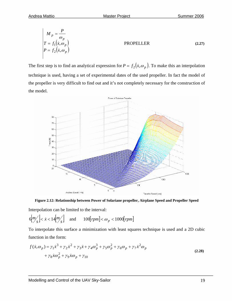
The first step is to find an analytical expression for ( )pxfP ω,2= . To make this an interpolation
technique is used, having a set of experimental dates of the used propeller. In fact the model of
the propeller is very difficult to find out and it’s not completely necessary for the construction of
the model.
Figure 2.12: Relationship between Power of Solariane propeller, Airplane Speed and Propeller Speed
Interpolation can be limited to the interval:
[ ] [ ]smxs
m 146 << and [ ] [ ]rpmrpm p 1000100 << ω
To interpolate this surface a minimization with least squares technique is used and a 2D cubic
function in the form:
1092
8
276
25
343
22
31),(
γωγωγ
ωγωγωγωγγγγω
+++
++++++=
pp
ppppp
xx
xxxxxf (2.28)

Andrea Mattio Master Project Summer 2006
Modelling and Control of the UAV Sky-Sailor
20
It’s possible to obtain a better result with a function of 4th order, but the difference is not big
enough to justify the use of a more complex model.
Figure 2.13: Power of Solariane Propeller interpolation
Once the analytical expression is obtained, it’s possible to develop some calculation and to find
an algebraic equation between pω (dependent variable) and 1U (independent variable).
( ) 0, 012
22 =⎟⎟⎠
⎞⎜⎜⎝
⎛ ⋅−⋅⋅−⋅+⋅
m
app
m
ap k
IRUrxP
kR
r ωηωηω (2.29)
Substituting ( ) ( )pp xfxP ωω ,, = one obtains an algebraic 3th order symbolic equation solvable
thanks to MatLab solve2.
023 =+++ dcba ppp ωωω (2.30)
( )( )( ) Im,
Im,Re,
133,
122,
111,
∈=∈=∈=
UxgUxgUxg
p
p
p
ωωω
(2.31)
2 It’s important to pay attention to the MatLab function solve because some time it gives strange results

Andrea Mattio Master Project Summer 2006
Modelling and Control of the UAV Sky-Sailor
21
The only possible solution is ( )111, ,Uxgp =ω because it’s the only real solution.
The second step is to find an analytical expression for ( )11 ,UxfT = . Following the same
procedure as before it’s easy to obtain the following relationship:
1092
8
276
25
343
22
31),(
σωσωσ
ωσωσωσωσσσσω
+++
++++++=
pp
ppppp
xx
xxxxxf (2.32)
Substituting this expression of ( )111, ,Uxgp =ω into ( )pxfT ω,1= , one finally finds out an
analytical expression ( )1,UxfT = .
Figure 2.14: Relationship between Thrust of Solariane Propeller, Motor Voltage and Airplane Speed
2.9 Simulink simulator
Once obtained a complete dynamic non linear model of the plane the following step is to
implement it under MatLab Simulink. The simulator is built:
• To simulate the behavior of the non linear model achieved
• To validate our model (for example comparing its behavior with the one of X-Plane)
• To design and test the controller
Andrea Mattio Master Project Summer 2006
Modelling and Control of the UAV Sky-Sailor
22
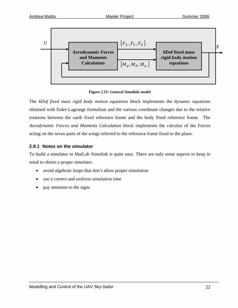
Figure 2.15: General Simulink model
The 6Dof fixed mass rigid body motion equations block implements the dynamic equations
obtained with Euler-Lagrange formalism and the various coordinate changes due to the relative
rotations between the earth fixed reference frame and the body fixed reference frame. The
Aerodynamic Forces and Moments Calculation block implements the calculus of the Forces
acting on the seven parts of the wings referred to the reference frame fixed to the plane.
2.9.1 Notes on the simulator To build a simulator in MatLab Simulink is quite easy. There are only some aspects to keep in
mind to obtain a proper simulator.
• avoid algebraic loops that don’t allow proper simulation
• use a correct and uniform simulation time
• pay attention to the signs
Aerodynamic Forces
and Moments Calculation
6Dof fixed mass
rigid body motion equations
[ ]ZYX FFF ,,
[ ]ψθφ MMM ,,
U X

Andrea Mattio Master Project Summer 2006
Modelling and Control of the UAV Sky-Sailor
23
3 Control model definition
Up to now a model useful for the simulation has been built. The next step is to build a model
suitable for the control. It’s so necessary to make some simplification and some change in order
to create a model that can be easily used to design a good controller for our system. Three main
changes have to be made.
• Interpolation of the Lift, Drag and Moment Coefficient
• Use of another Tait-Bryant angles sequence more suitable to the path tracking chosen
• Differential use of the ailerons
3.1 Lift, Drag and Moment Coefficient analysis
As said before the values for the airfoil coefficients are obtained thanks to specific software
(Javafoil). To build a control model it’s necessary to find out an analytical relationship between
the values of the aerodynamic coefficients and the independent variables (attack angle, Reynolds
number and aileron angle).
The relationships are quite difficult to express analytically. The solution chosen is the
interpolation. As usual some hypotheses have to be made:
• Reynolds number is considered constant and equal to 100000
• A range of aileron angle between -10° and 10° is considered
• A range of attack angle between -15° and 15° is considered
3.1.1 Lift and Moment coefficient interpolation
The process of interpolation for the lift and moment coefficients is very similar. In fact it’s easy
to see in the following figures that in the considered range both the lift and the moment
coefficients can be expressed as a linear 2D function of the attack angle and the flap angle.

Andrea Mattio Master Project Summer 2006
Modelling and Control of the UAV Sky-Sailor
24
Figure 3.1: Lift and Moment coefficients in the reduced range
The easiest way to find this relation is to interpolate this surface with a plane of equation:
321),( Δ+⋅Δ+⋅Δ= aaf αα (3.1)
α : angle of attack a : aileron flap angle iΔ : constant values
To find the values of iΔ there are different possibilities. The first and the simplest one is to find
a plane passing for three points of the surface. The second one is to interpolate the surface with a
plane exploiting the least squares method. In this case it has been chosen to use the first method
that, being more empirical, give better results.
Figure 3.2: Lift coefficient interpolation

Andrea Mattio Master Project Summer 2006
Modelling and Control of the UAV Sky-Sailor
25
Figure 3.3: Moment coefficient interpolation
3.1.2 Drag coefficient interpolation
For the Drag coefficient the situation is different. In fact the surface can’t be interpolate with a
linear 2D function.
Figure 3.4: Drag coefficient in the reduced range

Andrea Mattio Master Project Summer 2006
Modelling and Control of the UAV Sky-Sailor
26
The idea is to use a quadratic 2D function to interpolate this surface.
A general quadratic 2D function can be expressed as:
0'21)( fQf +⋅Γ+⋅⋅= λλλλ (3.2)
constfa
qqqq
Q
=
⎥⎦
⎤⎢⎣
⎡=
⎥⎦
⎤⎢⎣
⎡=Γ
⎥⎦
⎤⎢⎣
⎡=
0
2
1
21
1211
22
αλ
γγ
In order to find a function of this kind that fits well our surface a minimization technique as the
least squares or an empirical way can be used.
The disadvantage linked to the minimization with the least squares is that being a process purely
mathematical it’s possible to obtain values of the Drag coefficient that are inferior to zero, that is
physically impossible. So a way to find a good solution is to use a mix of the two techniques:
use of the least squares minimization and correction of the wrong values thanks to an empirical
and visual analysis.
Figure 3.5: Drag coefficient interpolation
Andrea Mattio Master Project Summer 2006
Modelling and Control of the UAV Sky-Sailor
27
3.2 New sequence of Tait-Bryant angles
The goal is to keep the plane flying consuming the minimum energy quantity. The strategy
chosen is to make it following a circle. So the plane it’s always in a turning configuration. If the
Tait-Bryant sequence seen in the previous chapter is used at each instant a variation of the
rotation matrix ( )ψθφ ,,R occurs. A possible solution is to use the following sequence:
( ) ( ) ( )⎥⎥⎥
⎦
⎤
⎢⎢⎢
⎣
⎡ −=
⎥⎥⎥
⎦
⎤
⎢⎢⎢
⎣
⎡
−=
⎥⎥⎥
⎦
⎤
⎢⎢⎢
⎣
⎡−=
1000cossin0sincos
,cos0sin
010sin0cos
,cossin0sincos0001
, ψψψψ
ψθθ
θθθ
φφφφφ zRyRxR
The new sequence used is the following:
( ) ( ) ( ) ( )θφψψθφ ,,,,, yRxRzRR ⋅⋅=
( )⎥⎥⎥
⎦
⎤
⎢⎢⎢
⎣
⎡=
φθφφθψφθψθψφψφθψθψφθψθψφψφθψθ
ψθφcoscossincossin-
cossincos-sinsincoscoscossinsin+sincossinsincos+cossinsincos-sinsinsin-coscos
,,R (3.3)
At the same time another relationship between the angular rates ),,( zyx ωωω and the
velocities ( )ψθφ ,, has to be found.
⎥⎥⎥
⎦
⎤
⎢⎢⎢
⎣
⎡
⋅⎥⎥⎥
⎦
⎤
⎢⎢⎢
⎣
⎡
⋅
⋅=
⎥⎥⎥
⎦
⎤
⎢⎢⎢
⎣
⎡
ψθφ
φθθφ
φθθ
ωωω
coscos0sinsin10
cossin-0cos
z
y
x
(3.4)
3.2.1 Relationship between the different sequences
It’s naturally useful to pass easily from one to another sequence. So it’s necessary to find a
transformation between the two sequences. The following notations will be used:
• ( )ststststR 1111 ,, ψθφ for the first sequence used to build the simulation model
• ( )ndndndndR 2222 ,, ψθφ for the second sequence used to build the control model
There is a set of ( )ndndnd 222 ,, ψθφ that describes the same orientation as the set of
angles ( )ststst 111 ,, ψθφ . The angles of course are different, but the orientations are the same. This
fact gives a way to convert angles in one scheme to or from angles in another. All nine of the
matrix elements are the same because the orientations are the same.
Using the following equality:

Andrea Mattio Master Project Summer 2006
Modelling and Control of the UAV Sky-Sailor
28
( ) ( )ststststndndndnd RR 11112222 ,,,, ψθφψθφ =
one can find a way to pass from one sequence to the other.
The used relationships are the following. All the calculations are reported in Appendix.
( )
⎟⎟⎠
⎞⎜⎜⎝
⎛⋅⋅+⋅⋅⋅−⋅
=
⎟⎠⎞⎜
⎝⎛
⋅=
⋅=
ststststst
stststststnd
ststst
nd
ststnd
11111
11112
111
2
112
sinsinsincoscossinsincoscossin
arctan
coscossinarctan
sincosarcsin
φθψφψφθψφψ
ψ
φθθθ
φθφ
(3.5)
To implement this transformation on the DSP that has a limited capacity calculus it’s possible to
linearize it, considering as correct the approximation of little angles for st1θ and st1φ . Making
this approximation:
⎟⎟⎠
⎞⎜⎜⎝
⎛⋅⋅+⋅⋅⋅−
=
==
stststst
ststststnd
stnd
stnd
1111
1112
12
12
sincoscossin
arctanφθψψφθψψ
ψ
θθφφ
(3.6)
3.3 Differential use of the ailerons
Another useful simplification is to suppose a differential use of the ailerons. This it made to
simplify the control action on the roll and to avoid strange correction of the controller on the
pitch or on the yaw using aileron flap. So on 23 UU −= and the system will be considered as a
system with 4 and not with 5 inputs.
⎥⎥⎥⎥⎥
⎦
⎤
⎢⎢⎢⎢⎢
⎣
⎡
−→−→
→→
=
right
leftnew
tailvUtailvU
aileronUmotorU
U
4
3
2
1
(3.7)

Andrea Mattio Master Project Summer 2006
Modelling and Control of the UAV Sky-Sailor
29
4 Control strategy
The control is organized in two different levels with different functions and different targets.
Low level control(LLC): Stability of the system
LQR(Linear Quadratic Regulator)
High level control(HLC): Path planning and tracking
Modern approach
Figure 4.1: Control strategy
The target of the inner loop is to keep the stability of the system, while the one of the outer loop
is to plan a path (in our case a circle) and to track it.
The Low Level Control has to satisfy the following main requirements:
• Keeping the global stability of the system
• Keeping a constant air speed
• Keeping a constant height
• Following the roll set point given by the HLC
• Keeping the stability also in presence of a wind, thought as a disturb
• Reducing as far as possible the energy consumption
• Minimizing the solicitations to the servo mechanism
The High Level Control instead:
• Path planning
• Path tracking
SKY-SAILORLLC HLC
Inner Loop
Outer Loop

Andrea Mattio Master Project Summer 2006
Modelling and Control of the UAV Sky-Sailor
30
4.1 Choice of a method for the Low Level Control (LLC)
The most used control method in the avionic field is the classical PID. The need in this case is to
have a control with the following requirements:
Robust and able to reject perturbations as wind or thermals
Possible to implement on a DSP without a great calculation power
The final choice is to use an optimal linear state feedback control method based on the built
dynamic and aerodynamic model and in particular a LQR (Linear Quadratic Regulator).
4.2 Choice of a method for the High Level Control (HLC)
The target to achieve is to keep the plane flying following a specified path with low energy
consumption. The choice is to follow a circular path with a large diameter in order to avoid
shocks on the commands (ailerons, v-tails and motor) and to reduce wind influence.
In literature there are a lot of papers proposing method to achieve this goal. As usual the
problem is to use a control method requiring a little calculation power and easy to implement.
The choice is to adapt an algorithm [3] proposed and tested for the path tracking of a non-
holonomous robot.

Andrea Mattio Master Project Summer 2006
Modelling and Control of the UAV Sky-Sailor
31
5 Model linearization
To design the control a linear model of the system is needed. This linear model will be naturally
correct only around the so-called steady-state point, which has to be found.
The steps to achieve are:
• Finding the steady-state point
• Linearize the model around this point
5.1 Search of a steady-state point
5.1.1 Steady-state point for a straight flight
The final non-linear model obtained thanks to modeling process is in the form:
),( UXfX = (5.1)
⎥⎥⎥⎥
⎦
⎤
⎢⎢⎢⎢
⎣
⎡
=
⎥⎥⎥⎥⎥⎥⎥⎥⎥⎥⎥⎥⎥⎥⎥⎥⎥
⎦
⎤
⎢⎢⎢⎢⎢⎢⎢⎢⎢⎢⎢⎢⎢⎢⎢⎢⎢
⎣
⎡
=
4
3
2
1
UUUU
Uzyxzyx
X E
E
E
E
E
E
ψθφψθφ
The goal is to find a particular configuration of X and U for which a steady-state solution of the
equation (5.1) is obtained, that means:
)~,~(0 UXf= (5.2)
First some hypotheses can be made to simplify the problem. All these hypotheses are made on
the base of physical considerations about airplane behavior during his flight.

Andrea Mattio Master Project Summer 2006
Modelling and Control of the UAV Sky-Sailor
32
???
===
E
E
E
zyx
(5.3)
They are insignificant for the search of the steady-state point because they don’t influence the
dynamic behavior of the airplane. The part of the model describing the evolution of the position
of the airplane in the Earth fixed reference frame is totally decoupled in respect of the part of the
model describing the evolution of the other states.
0?0
===
ψθφ
(5.4)
The airplane in its steady-state configuration should have a roll and a yaw angle equal to zero.
Anything is known about the pitch angle. The pitch angle influences the angle of attack of the
airplane so it’s a free parameter.
Figure 5.1: Plane angles configuration
00?
===
E
E
E
zyx
(5.5)
The speed Ex is approximately [ ]sm2.8 from considerations coming from the reality. Anyway
this is surely a free parameter in the search of the steady-state point.
z
x
y
roll
yaw
pitch

Andrea Mattio Master Project Summer 2006
Modelling and Control of the UAV Sky-Sailor
33
000
===
ψθφ
(5.6)
It’s quite evident that the angular rates should be equal to zero.
For the inputs U the reasonable hypotheses that at the steady-state point the aileron are closed
can be made. The motor voltage instead can be considered as a free parameter. Anyway also in
this case some information about the possible range of values for the parameter 1U is available.
The plane has a glide slope in a stable situation of approximately 25. With a simple calculation:
NgMslopeglideT 1
8.96.225_
≈⋅
=⋅
=
Looking at figure (1.21) one can see that this corresponds to a motor voltage of
approximately V19 . This calculation is just an indication and it’s not a reference to judge the
results.
000?
4
3
2
1
====
UUUU
(5.7)
5.1.1.1 Steady-state point empirical search
One important characteristic of Sky-Sailor is that is auto-stable. So a first essay to find an
indication about the steady-state point is to simulate with the MatLab Simulink simulator the
free behavior of the airplane.
Simulating the free behavior of the airplane with the initial conditions found before it’s possible
to see that after an initial transitory the Sky-Sailor reaches a stable situation.
First the motor voltage is set equal to zero that it means that the airplane is left in a situation of
free fall and the following results are obtained:

Andrea Mattio Master Project Summer 2006
Modelling and Control of the UAV Sky-Sailor
34
Figure 5.2: θ evolution in free fall condition
After some beginning oscillations the airplane stabilizes itself for an angle °−= 8.3θ .
Figure 5.3: zE evolution in free fall condition

Andrea Mattio Master Project Summer 2006
Modelling and Control of the UAV Sky-Sailor
35
For the position Ez in sec150 the plane falls of approximately m50 . One can make an
estimation of the fall speed that is sec3.0sec150
50 mmz ≈= . This result is indicative but it’s quite
similar to the one obtained during the tests with the real plane.
For the speed a value of sec4.8 mxe = is found that it’s quite consistent with the values obtained
in the reality.
Then a motor voltage is put in order to observe the behavior of the airplane. A motor voltage
of V19 is set because it’s approximately the voltage necessary to allow the airplane to fly in a
steady-state condition.
Figure 5.4: θ evolution with motor voltage =19V
In this situation an angle °−= 5.1θ is obtained. The optimal situation should be an angle of -1°,
because of the particular configuration and disposition of the v-tail. So one can conclude that
thanks to the built model a static behavior similar to the real one is found.
A speed sec5.8 mxe = that is quite consistent with real experiments is found.

Andrea Mattio Master Project Summer 2006
Modelling and Control of the UAV Sky-Sailor
36
5.1.1.2 Steady-state point mathematical search
A second possible approach to find the steady-state point is a mathematical approach thanks to
an optimization procedure. The starting point is the non-linear model ),( UXfX = . In this
model the following values are imposed:
0~0
~0
~0~0~
0~0~
===
====
ψθφ
ψφ
E
E
zy
0~0~0~0~
4
3
2
1
====
UUUU
(5.8)
The free parameters are:
?~?~?~
1 ===
U
xE
θ (5.9)
The goal is to find the values of these free parameters that minimize the cost function: 2222 ψθφ +++++= EEE zyxJ (5.10)
This procedure is realized thanks to the MatLab function fmincon. The result obtained is:
18.9054V~-1.5012~ sec
m8.5245~
1 =°=
=
U
xE
θ
These results are quite consistent with those obtained with the empirical method, so one can
conclude that the steady-state point found is reasonable and it reflects quite well the behavior of
the real system.
5.1.2 Steady-state point for a circular flight
As said before the goal is to keep the plane flying following a circular path. In these flight
conditions is better to fin a steady-state point appropriate. The procedure is similar to the one
used in the chapter 5.1.1.
The parameters imposed are the following:

Andrea Mattio Master Project Summer 2006
Modelling and Control of the UAV Sky-Sailor
37
Ex
cR
y
x
0000
5.80~
====
==
θφ
ψ
E
E
E
zy
smx
(5.11)
The free parameters are:
?~?~?~?~??~?~
4
3
2
1
=======
UUUUψθφ
(5.12)
In this case the cost function J is more complicated than (5.11).
( ) ( ) ( ) 222
24
23
221
222 ~~~ailrollEctEE FWUUUWzayxJ −⋅+++⋅+++++−+= ψθφ (5.13)
The acceleration along Ey has to be modified because of the fact that the plane is turning, so
it’s influenced by a centripetal acceleration. To estimate in an easy way this term one can have a
look at the following figure:
Figure 5.5: Evaluation centripetal acceleration
It’s easy to see that the acceleration along Ey will be equal to the centripetal acceleration, which
can be estimated as:
Andrea Mattio Master Project Summer 2006
Modelling and Control of the UAV Sky-Sailor
38
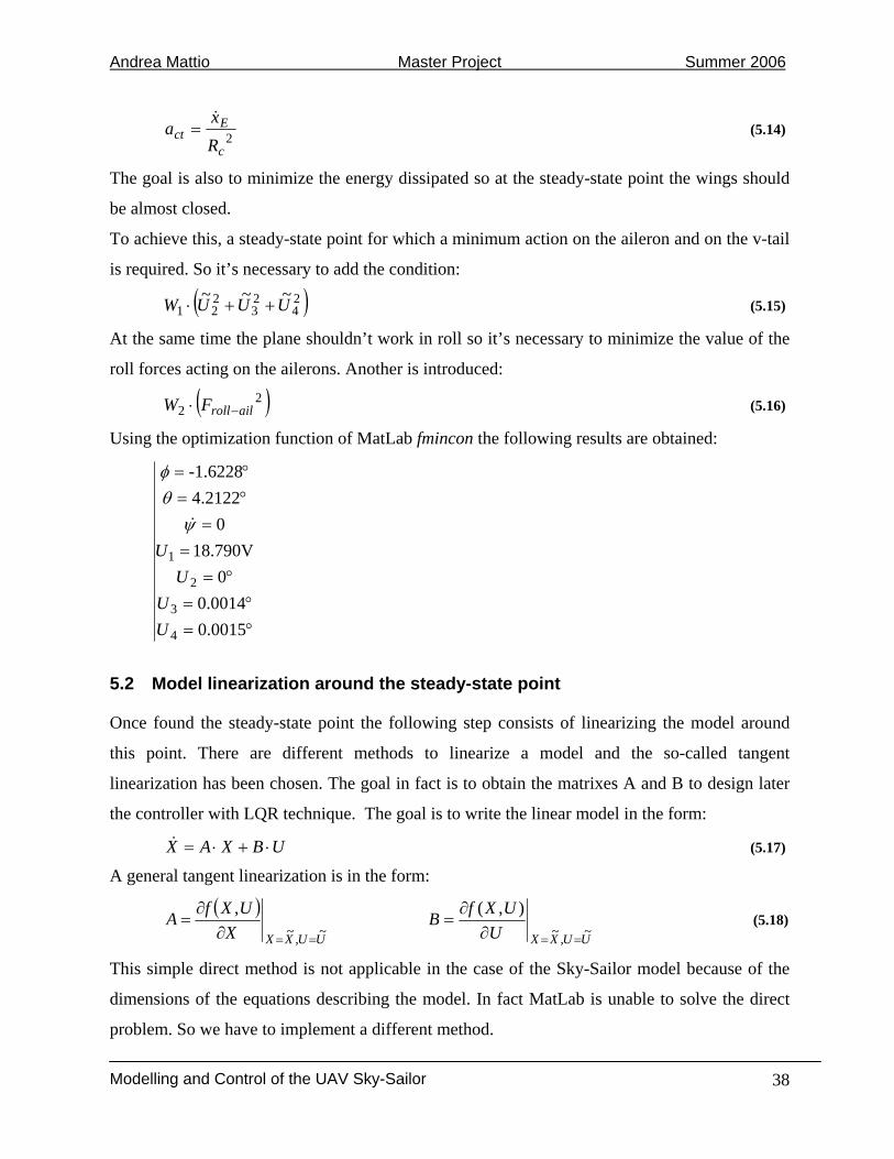
2c
Ect
Rx
a = (5.14)
The goal is also to minimize the energy dissipated so at the steady-state point the wings should
be almost closed.
To achieve this, a steady-state point for which a minimum action on the aileron and on the v-tail
is required. So it’s necessary to add the condition:
( )24
23
221
~~~ UUUW ++⋅ (5.15)
At the same time the plane shouldn’t work in roll so it’s necessary to minimize the value of the
roll forces acting on the ailerons. Another is introduced:
( )22 ailrollFW −⋅ (5.16)
Using the optimization function of MatLab fmincon the following results are obtained:
°=°=
°==
=°=°=
0.00150.0014
018.790V
04.2122-1.6228
4
3
2
1
UU
UU
ψθφ
5.2 Model linearization around the steady-state point
Once found the steady-state point the following step consists of linearizing the model around
this point. There are different methods to linearize a model and the so-called tangent
linearization has been chosen. The goal in fact is to obtain the matrixes A and B to design later
the controller with LQR technique. The goal is to write the linear model in the form:
UBXAX ⋅+⋅= (5.17)
A general tangent linearization is in the form:
( )UUXXX
UXfA~,~
,
==∂∂
= UUXXU
UXfB~,~
),(
==∂∂
= (5.18)
This simple direct method is not applicable in the case of the Sky-Sailor model because of the
dimensions of the equations describing the model. In fact MatLab is unable to solve the direct
problem. So we have to implement a different method.

Andrea Mattio Master Project Summer 2006
Modelling and Control of the UAV Sky-Sailor
39
A possible solution is to split the calculation in different little calculations.
( )
( )( )
( )( )
( )( )
( )( ) MMFFUUXX
MMFFUUXX
MMFFUUXXUUXX
MFXUXM
UXMUXf
MFXUXF
UXFUXf
MFXUXf
XUXfA
~,~,~,~
~,~,~,~
~,~,~,~~,
,,
,,
,,
,,
),(),(),
====
====
======
∂∂⋅
∂∂
+∂∂
⋅∂∂
+∂∂
=∂
∂=
(5.19)
( ) ( ) ( )( ) ( )∑ ∑
= =⎟⎟⎠
⎞⎜⎜⎝
⎛
∂∂
=∂∂
⇒=7
1
7
1,
,),(,,,
i iii UXF
MFXMFXUXFUXFUXF (5.20)
For the linearity of the sum and the derivation one can write:
( ) ( ) ( )( )∑∑
==⎟⎟⎠
⎞⎜⎜⎝
⎛∂∂
=⎟⎟⎠
⎞⎜⎜⎝
⎛
∂∂ 7
1
7
1 ,,
,, i ii
i
ii MFX
UXFUXF
MFX (5.21)
( )
( )( )
( )( )
( )( )
( )( )∑
∑
= ====
= ====
======
⎟⎟
⎠
⎞
⎜⎜
⎝
⎛
∂∂⋅
∂∂
+⎟⎟
⎠
⎞
⎜⎜
⎝
⎛
∂∂
⋅∂∂
+∂∂
=∂
∂=
7
1 ~,~,~,~
7
1 ~,~,~,~
~,~,~,~~,
,,
,,
,,
,,
),(),(),
i iMiMiFiFUUXXii
i
i
i iMiMiFiFUUXXii
i
i
MMFFUUXXUUXX
MFXUXM
UXMUXf
MFXUXF
UXFUXf
MFXUXf
XUXfA
(5.22)
Unfortunately this simplification is not sufficient. It’s necessary to go deeper in this procedure.
( )( )
( )( )
( )( )
( )( )
( )( )
( )( )
( )( )
( )( )
MiCMiCDiCDiCLiCLiCiMiMiFiFUUXXMiDiLi
Mi
Mi
i
MiCMiCDiCDiCLiCLiCiMiMiFiFUUXXMiDiLi
Di
Di
i
MiCMiCDiCDiCLiCLiCiMiMiFiFUUXXMiDiLi
Li
Li
i
MiCMiCDiCDiCLiCLiCiMiMiFiFUUXXMiDiLi
i
ii
i
CCCXUXC
UXCUXF
CCCXUXC
UXCUXF
CCCXUXC
UXCUXF
CCCXUXF
MFXUXF
~,~,~,~,~,~,~
~,~,~,~,~,~,~
~,~,~,~,~,~,~
~,~,~,~,~,~,~
,,,
,,
,,,
,,
,,,
,,
,,,
,,
=======
=======
=======
=======
∂∂
⋅∂∂
+∂
∂⋅
∂∂
+∂
∂⋅
∂∂
+∂
∂=
∂∂
(5.23)
Andrea Mattio Master Project Summer 2006
Modelling and Control of the UAV Sky-Sailor
40
Substituting 4.17 in 4.16 the final relation that leads to the matrix A of the linear model can be
found.
The same procedure is used also to build the matrix B. But for the matrix B is sufficient to stop
this procedure at a higher level.
( )
( )( )
( )( )
( )( )
( )( ) MMFFUUXX
MMFFUUXX
MMFFUUXXUUXX
MFUUXM
UXMUXf
MFUUXF
UXFUXf
MFUUXf
UUXfB
~,~,~,~
~,~,~,~
~,~,~,~~,
,,
,,
,,
,,
),(),(),
====
====
======
∂∂⋅
∂∂
+∂∂
⋅∂∂
+∂∂
=∂
∂=
(5.24)
Implementing this algorithm in MatLab it’s possible to arrive at the solution of the problem
finding the matrix A and B of the linear model around the steady-state point found before.

Andrea Mattio Master Project Summer 2006
Modelling and Control of the UAV Sky-Sailor
41
6 Low level control: Linear Quadratic Regulator
6.1 Linear quadratic control
Linear quadratic control is a technique of optimal state feedback control.
Each linear or linearized system can be written in the form:
)()()()()()(tDutCxtytButAxtx
+=+=
(6.1)
The Linear Quadratic Control consists of finding a static matrix K in order to find the input to
the system:
)()( txKtu ⋅−= (6.2)
that has to stabilize the system and to minimize the cost function:
( )∫∞
+=0
dtRuuQxxJ TT (6.3)
where Q and R are two weight matrixes which obey to the following constraints:
0≥= TQQ 0≥= TRR (6.4)
We can find the solution:
PBRK T1−= (6.5)
where P is solution of the Riccati equation:
PQPBPBRPAPA TT =++−− −1 (6.6)
It’s possible to consider a steady-state solution of this equation, as usually made in literature. So
the equation to solve is:
01 =+−+ − QPBPBRPAPA TT (6.7)
6.2 Solution of Riccati equation
Now the problem is to solve the Riccati equation 5.7. A general Riccati equation can be written
as:
0=−−+ rrrr CXDXAXXB (6.8)
where:
Andrea Mattio Master Project Summer 2006
Modelling and Control of the UAV Sky-Sailor
42
[ ][ ][ ]mxnCnxmBnxnA
r
r
r
===
[ ][ ]mxnX
mxmDr
==
The Hamiltonian matrix can be built:
⎥⎦
⎤⎢⎣
⎡=
rr
rr
DCBA
H (6.9)
that in this case is equivalent to:
⎥⎥⎦
⎤
⎢⎢⎣
⎡
−−−=
−
T
T
AQBBRAH
1 (6.10)
It’s possible to demonstrate that the 2n eigenvalues of H are the n eigenvalues of the closed
loop matrix KBA ⋅− and their opposites. Finally if λ is an eigenvalue of H , it’s sure that
λ− will be too.
So it exists n and only n eigenvalues whose real part is negative. If ( )ndiag λλ ...1=Λ is the
matrix of the eigenvalues one can build the matrix [ ]nxnX 2= , made of eigenvectors and one
obtains the following important relationship:
Λ= XHX (6.11)
Finally, it’s possible to divide X in two matrixes 1X and 2X and to demonstrate that P desired,
solution of the Riccati equation, is in the form: 1
12−= XXP (6.12)
6.3 Linear Quadratic Regulator for Sky-Sailor
6.3.1 Model Reduction
The final linearized model of the system is in the form:
DUCXYBUAXX
+=+= (6.13)
where:
[ ][ ]4321 UUUUU
zyxzyxX EEEEEE
== ψθφψθφ
(6.14)

Andrea Mattio Master Project Summer 2006
Modelling and Control of the UAV Sky-Sailor
43
In reality it’s not necessary to control all the states of this model but, at the same time, it’s
necessary to control some state which is not in this model. To make it possible a space-
transformation can be made in order to project the system in the desired space of controllability.
So the transformation:
XX Γ=ˆ (6.15)
is made with:
[ ]θφθφ EeeE zyxzX =ˆ (6.16)
The states that must be controlled are:
→φ Roll
→θ Pitch
→Ez Altitude
→ex Air speed
→ey Lateral slip
The other three states are considered in this model reduced to maintain the mathematical
controllability of the system.
The transformation matrix Γ should be well-conditioned and non-singular ( ( ) 0det ≠Γ ). It’s
possible to demonstrate that the following matrix is well-conditioned and non –singular.
⎥⎥⎥⎥⎥⎥⎥⎥⎥⎥⎥⎥⎥⎥⎥⎥⎥
⎦
⎤
⎢⎢⎢⎢⎢⎢⎢⎢⎢⎢⎢⎢⎢⎢⎢⎢⎢
⎣
⎡
⋅⋅⋅⋅⋅+⋅⋅⋅⋅
=Γ
000000100000100000000000000000000010000000000001010000000000001000000000000100000000000sincoscossincos-000000000cossin-cossinsinsincossinsinsin-coscos000000000000000100000000010000000000001000
φψφψφφθψφθψθψφθψθ
Inversing (6.15) one obtains:
XX ˆ1−Γ= (6.17)

Andrea Mattio Master Project Summer 2006
Modelling and Control of the UAV Sky-Sailor
44
Considering the matrix Γ evaluated in the steady-state point one obtains a numerical matrix and
it’s possible to conclude that:
XX ˆ1−Γ= (6.18) Substituting in (6.13):
BUXAX +Γ=Γ −− ˆˆ 11 (6.19)
BUXAX Γ+ΓΓ= − ˆˆ 1 (6.20)
The target is finally achieved because a reduced model is obtained in the form:
UBXAX ˆˆˆˆˆ += (6.21)
⎥⎥⎥⎥⎥⎥⎥⎥⎥⎥⎥
⎦
⎤
⎢⎢⎢⎢⎢⎢⎢⎢⎢⎢⎢
⎣
⎡
−−−−−−
−−−−−−−
−−−−=
3960.111934.05325.66869.00273.003697.550051.00002.07165.200001.08554.2000012.001722.00529.03078.85836.02593.205835.707601.007208.003623.00006139.90199.01049.04168.00100.02386.001230.60001000001000000001000000
A (6.22)
⎥⎥⎥⎥⎥⎥⎥⎥⎥⎥⎥
⎦
⎤
⎢⎢⎢⎢⎢⎢⎢⎢⎢⎢⎢
⎣
⎡
−−−−−−−−−
=
03972.330015.361946.100021.20034.24561.104
0024.01598.29405.12099.004931.14931.18575.2
0852.00503.00503.00000000000000
B (6.23)
6.3.2 Analysis of controllability
The first thing to make is to check if the reduced model is controllable or not.
A system is controllable if:
( ) →= nQrank System dimension
where :

Andrea Mattio Master Project Summer 2006
Modelling and Control of the UAV Sky-Sailor
45
[ ]→= − BABAABBQ n 12 ... Controllability matrix
To check the controllability is sufficient to use the MatLab instruction ctrb3.
With this analysis it’s possible to find out that the system is controllable
6.3.3 Choice of Q and R
As one can read in literature it doesn’t exist a methodical approach for the choice of the weight
matrixes Q and R. This is the weak point of this control method and it’s the point that adds a
difficulty to a method apparently so easy to use.
First it’s good thing to choice to use only diagonal matrixes in order to simplify the control
design.
)( iqdiagQ = with 8=i
)( jrdiagR = with 4=j
The choice has been made observing the behavior of the control in simulation. The goal is to
design a control with the following characteristics:
• Air speed always constant with a few variations allowed
• Robust to wind disturbs
• Action on the ailerons as slighter as possible
• Motor use reasonable
Finally a good choice for the matrixes is the following:
⎥⎥⎥⎥⎥⎥⎥⎥⎥⎥⎥
⎦
⎤
⎢⎢⎢⎢⎢⎢⎢⎢⎢⎢⎢
⎣
⎡
=
1000000005.0000000001000000000300000000005000000000500000000001.0000000001500
Q (6.24)
3One can read in MatLab help that:”Estimating the rank of the controllability matrix is ill-conditioned; that is, it is very sensitive to roundoff errors and errors in the data.” So it’s preferable to use ctrbf for problems of big dimensions

Andrea Mattio Master Project Summer 2006
Modelling and Control of the UAV Sky-Sailor
46
⎥⎥⎥⎥
⎦
⎤
⎢⎢⎢⎢
⎣
⎡
=
1000010000001000000100
R (6.25)
The control obtained behaves quite well as far as concerns the stability4.
6.3.4 LQR with integral action
With the LQR control a static error on some states appears. In particular a static error on the air-
speed Ex , on the roll φ is present. This error can be quite negative for the control behavior so
it’s necessary to correct it. The possible solution is to add an integral term.
One way of forcing integral action is to put a set of integrators at the output of the plant. In other
words adding an integral term in a state-feedback control method means augmenting the system.
This can be described in a state-space form as:
( ) ( ) ( )( ) ( )( ) ( ) )(trtytz
tCxtytButAxtx
−==
+= (6.26)
The composite system becomes:
( ) ( ) ( )tuBtxAtx ′′+′′=′ (6.27)
where:
( ) ( )( )⎥⎦⎤
⎢⎣
⎡=′
tztx
tx ⎥⎦
⎤⎢⎣
⎡=′
00
CA
A ⎥⎦
⎤⎢⎣
⎡=′
0B
B (6.28)
Then the goal is to find the gain K ′ that stabilizes this augmented system.
In the system an integral action is put on:
→φ Roll
→ex Air speed
So the augmented system (6.27) is built, the controllability is checked and the good matrixes Q’
and R’ are found.
This technique has the advantage of being robust to variations in system matrix (A,B,C,D) that
are used to compute the steady-state point.
4 All the figures concerning intermediate results are reported in the Annexes

Andrea Mattio Master Project Summer 2006
Modelling and Control of the UAV Sky-Sailor
47
⎥⎥⎥⎥⎥⎥⎥⎥⎥⎥⎥⎥⎥
⎦
⎤
⎢⎢⎢⎢⎢⎢⎢⎢⎢⎢⎢⎢⎢
⎣
⎡
=′
0000
0000000100001000
0000000000000000
AA (6.29)
⎥⎥⎥⎥
⎦
⎤
⎢⎢⎢⎢
⎣
⎡
=′
00000000
B
B (6.30)
It’s easy to find out that the augmented system is controllable and after some trial good matrixes
Q’ and R’ are found for the new system. The aspects to consider in designing this controller are
the same made in the previous chapter.
⎥⎥⎥⎥⎥⎥⎥⎥⎥⎥⎥⎥⎥⎥
⎦
⎤
⎢⎢⎢⎢⎢⎢⎢⎢⎢⎢⎢⎢⎢⎢
⎣
⎡
=′
5000000000005.000000000001000000000010000000000001.0000000000010000000000030000000000020000000000010000000000300
Q (6.31)
⎥⎥⎥⎥
⎦
⎤
⎢⎢⎢⎢
⎣
⎡
=′
1000010000001000000100
R (6.32)

Andrea Mattio Master Project Summer 2006
Modelling and Control of the UAV Sky-Sailor
48
The final control that will be tested in simulation and implemented on the real system is the
following:
⎥⎥⎥⎥
⎦
⎤
⎢⎢⎢⎢
⎣
⎡
−−−−−−−−−−
−−−−−−−
=′
2890.04192.00562.00002.01478.09803.34815.30814.17714.02500.00364.00836.00048.01209.02366.01268.00527.13330.02486.00338.00906.00034.01073.01952.02106.01438.12603.0
2369.00011.00003.02128.00327.00117.00176.00049.00358.1
K

Andrea Mattio Master Project Summer 2006
Modelling and Control of the UAV Sky-Sailor
49
CENTER
RADIUS
x
y
7 High level control
The target of the outer loop is to give an appropriate set point to the inner loop in order to be
able to follow the desired path. The idea is to follow a simple path, without consuming a lot of
energy and avoiding the problems relied to the wind. The path chosen is a circle; in particular a
point expressed in GPS coordinates, which is the circle centre, and a radius are assigned to the
HLC, which has to track the desired circle. The HLC should be able to track the path also in
presence of wind.
Figure 7.1: Path planning for the HLC
Considering the position of the centre and the radius of the circle it creates the reference path.
Comparing the real position and the real heading with the desired position it generates the value
of heading necessary to achieve the desired position.
The heading value is taken as input of a PI controller in order to generate the roll set point which
is communicated to the LLC.
Figure 7.2: HLC strategy
Reference Path generation
Heading generator PI
radius
( )cc yx ,
Heading GPS
( )GPSGPS yx , Heading SP
Roll SP

Andrea Mattio Master Project Summer 2006
Modelling and Control of the UAV Sky-Sailor
50
7.1 Heading generator
7.1.1 Velocity scheduling controller for a nonholonomic mobile robot [3]
The heading generator constitutes a revision, an adaptation to the plane of the “Velocity
Scheduling Controller for a nonholonomic mobile robot”, realized at the Automatic Laboratory
of the EPFL (École Polytechnique Fédérale de Lausanne).
The concept is to compare the behavior of a nonholonomic mobile robot with the behavior of
our plane.
7.1.1.1 Nonholonomic mobile robot vs Sky-Sailor
Consider a mobile robot moving on a planar surface where 1x is the horizontal coordinate and
2x the vertical one. The angle that the robot makes with the horizontal axes is 3x . The kinematic
equations of motions are given by:
( )( )
23
312
311
sincos
vxxvxxvx
===
(7.1)
where 1v and 2v are the inputs; 1v denotes the velocity in the direction defined by the heading
angle and 2v the angular velocity.
The idea is that a plane moving at a given height, with a given and fixed angle of attack can be
described by the same kinematic equations of a nonholonomic robot (7.1). In fact we can write:
( )( )ϕϕ
sincos⋅=⋅=
eE
eE
xyxx
(7.2)
where ϕ 5 is the input; ex denotes the air speed of the plane, Ex and Ey the positions in the GPS
reference frame.
Exploiting this equality the same algorithm implemented for the nonholonomic mobile robot can
be used also for Sky-Sailor. The only difference is that, while for the robot 1v can be used as an
input and it’s possible to act on it to achieve the target, for the plane this is not possible because
5 ϕ is the heading and it’s defined as the direction of the velocity vector, so it can be mathematically derived as
⎟⎠⎞⎜
⎝⎛=
EE
xyarctanϕ

Andrea Mattio Master Project Summer 2006
Modelling and Control of the UAV Sky-Sailor
51
Roll SP Heading SP PI
the air speed ex is a parameter to control carefully. So the same algorithm can be used but it’s
mandatory to block the action on the velocity.
The proposed controller is the following:
7.1.2 From heading to roll set point
Once the heading value necessary to track properly the trajectory is generated, it’s necessary to
convert it into a value suitable for the Low Level Control. The easiest thing to do is to convert it
into a roll reference. In fact to track a heading position the easiest thing is to rotate along the
longitudinal axes of the plane that in this case is represented by the x axes. But a rotation around
x axes corresponds to a modification of the roll. So it’s easy to transform the heading reference
into a roll reference simply with a proportional gain. In reality to avoid static errors it’s chosen
to design a simple PI controller in order to pass from heading to roll set point.
Figure 7.3: From heading to roll set point
Circle trajectory generation freq = set_pt_wind_speed_f / (2*PI*radius); sin_traj = sin(2*freq*PI*time); cos_traj = cos(2*freq*PI*time); x1 = radius*cos_traj; x1d = -2*freq*PI*radius*sin_traj; x1dd = -4*freq*freq*PI*PI*radius*cos_traj; x2 = radius*sin_traj; x2d = 2*freq*PI*radius*cos_traj; x2dd = -4*freq*freq*PI*PI*radius*sin_traj; Heading generator
chi1_kplus1 = (-k*k*k*int1 - 3*k*k*(latitude_rel_meter -x1) - 3*k*(chi1-x1d) + x1dd) * 1 + chi1;
chi2_kplus1 = (-k*k*k*int2 - 3*k*k*(longitude_rel_meter-x2) - 3*k*(chi2-x2d) + x2dd) * 1 + chi2;
int1_kplus1 = (latitude- x1) * 1 + int1; int2_kplus1 = (longitude-x2) * 1 + int2; x3_hat = atan2(chi2,chi1); last_errx3 = errx3; errx3 = atan2(sin(x3_hat-heading_gps),cos(x3_hat-heading_gps));

Andrea Mattio Master Project Summer 2006
Modelling and Control of the UAV Sky-Sailor
52
8 HLC and LLC fusion: simulation The last target to achieve consists of fusing HLC and LLC together in order to have a total
autonomous control of the plane. The integration of two controls doesn’t consist only of a
simple superposition of the two levels but also in a careful analysis of the relationships between
the two controllers and of the effects of one on the other.
In this case the integration has lead to make some variations to the LLC, in particular to vary
some weight in order to achieve a better behavior of the system.
• Design of a control which doesn’t solicit to much the servo-mechanism. This design is
made thanks to the Fourier analysis of the input signals of the system.6
• Saturation on ( )maxzzz < to lighten the control and to avoid abrupt changes on the
physical inputs of the system.
• Filtering on the input values given to the system to avoid high frequencies solicitations
of the servo-mechanism.
8.1 Altitude saturation and commands filter Altitude saturation is necessary to lighten control action and aggressiveness. Being an optimal
but always a proportional controller, LQR reacts in a very aggressive manner in front of
important errors on the states. This is really dangerous in the case of the altitude for the global
behavior of the system; in fact the risk of going in instability it’s great. For that reason it’s useful
to saturate the value of the altitude.
Figure 8.1: Altitude control with and without saturation
6 The results of this analysis are reported in the Annexes

Andrea Mattio Master Project Summer 2006
Modelling and Control of the UAV Sky-Sailor
53
Figure 8.2: Total path without and with saturation
A filter on the commands is useful in order to reduce the solicitations on the servos. But at the
same it’s a very delicate point to touch. In fact design a wrong filter on the commands means
to lead the system to instability. The chosen one is a Butterworth first order filter with a cut
frequency of 3Hz. This frequency has been chosen because it’s more or less the maximum
excited frequency for the servos.
8.2 Necessity of a HLC The first simple idea to follow a circular path is to give a constant roll to the plane in order to
make it turning. This technique, being simple and easy to implement, is not adapt to Sky-Sailor.
In fact in presence of a little constant wind (1m/sec in X direction) the system behavior is really
different to the hoped one.
Figure 8.3: Plane behavior in presence of a constant wind with only LLC control

Andrea Mattio Master Project Summer 2006
Modelling and Control of the UAV Sky-Sailor
54
The plane begins to fly following a spiral; this is why a HLC control is necessary. In fact with
the insertion of the HLC control in the same wind situation the plane behavior is really better.
Figure 8.4: Plane behavior in presence of a constant wind with HLC and LLCcontrol
HLC control takes one or two rounds to fit well the circle but then also in presence of a wind it’s
able to keep the desired circular path.
8.3 Sky-Sailor behavior in simulation Thanks to Simulink simulator it’s possible to analyze the behavior of the plane in absence and in
presence of the wind. At the same it’s also possible to simulate the noise present on the sensors
measures and so to understand quite well the possible real behavior of Sky-Sailor.
It’s important to underline that the wind is modeled in a quite simple way: wind influence is
simulated as an increment or a reduction on the plane speed in the earth reference frame.
Figure 8.5: wind simulated

Andrea Mattio Master Project Summer 2006
Modelling and Control of the UAV Sky-Sailor
55
8.3.1 Without wind disturbs Simulations are first made without considering wind disturbs. In this first simulation the plane
has the initial conditions:
mxmzmxe 10013070sec2.8 =−=°== ψ
Figure 8.6: HLC and LLC control without wind disturbs
While LLC keeps the stability of the plane and controls the altitude, HLC works to achieve the
circle. This is evident looking at the following two figures, representing the plane x-z, so LLC
action and the plane x-y so HLC action.
Figure 8.7: x-y and x-z planes

Andrea Mattio Master Project Summer 2006
Modelling and Control of the UAV Sky-Sailor
56
It’s possible to conclude that HLC-LLC fusion control works quite well in absence of wind. It’s
interesting to analyze also the influence as far as concerns solicitations to the servos.
Figure 8.8: Servos solicitations
8.3.2 With wind disturbs Second simulation has been made considering wind effect and in particular wind has been
simulated as in figure 8.3. The initial conditions are the same that for the previous simulation.
Figure 8.9: HLC and LLC control with wind disturbs

Andrea Mattio Master Project Summer 2006
Modelling and Control of the UAV Sky-Sailor
57
System behavior is quite good considering flight difficult conditions. This simulation shows a
good robustness of the total control.
Figure 8.10: x-y and x-z planes
Figure 8.11: Controlled altitude
Once more it’s possible to say that total control has a correct behavior also in presence of a quite
strong wind. In fact if one considers that the plane flies with a constant speed of 8.2 m/sec, the
wind is equal to:
%4.24100sec2.8
sec2%_ =⋅=
m
mstrengthwind

Andrea Mattio Master Project Summer 2006
Modelling and Control of the UAV Sky-Sailor
58
For servos solicitations it’s possible to see that wind disturbs leads to an augmentation of them.
Figure 8.12: Solicitations in wind presence
Anyway it’s right to conclude that these solicitations are sustainable for the plane also because
the goal is to fly in good weather situations and not in presence of repeated wind flows.

Andrea Mattio Master Project Summer 2006
Modelling and Control of the UAV Sky-Sailor
59
9 Embedded system on Sky-Sailor The main components of the embedded system on Sky-Sailor are:
• DSPIC: it constitutes the heart of the embedded system, where all the information is
collected and where the control is implemented. This element has a calculation power
not so elevated and this constitutes one of the main challenges in the control design.
• ONBOARD SENSORS: they constitute the receptors of the system and they allowed
the knowledge of all the useful information for the control
• BUS I2C: it allows communication between some sensor and DSPIC
• RADIO MODEM: it’s used for the communication between the ground and the plane
Figure 9.1: Embedded system on Sky-Sailor
Andrea Mattio Master Project Summer 2006
Modelling and Control of the UAV Sky-Sailor
60
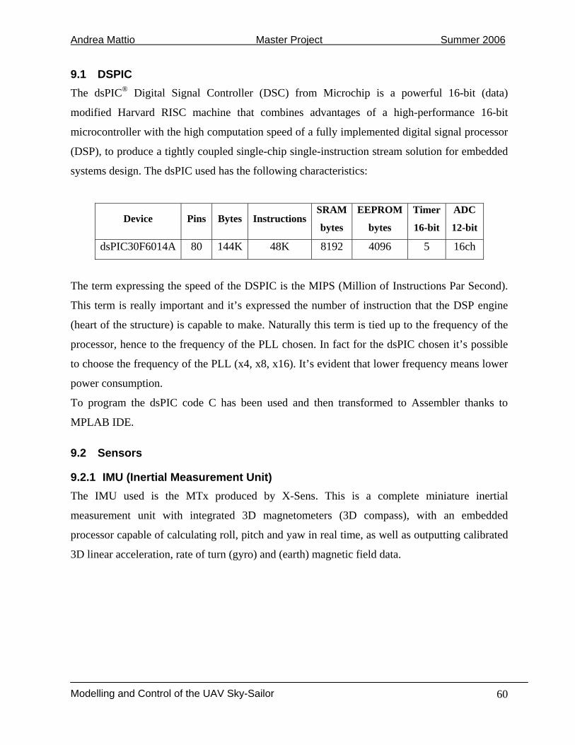
9.1 DSPIC The dsPIC® Digital Signal Controller (DSC) from Microchip is a powerful 16-bit (data)
modified Harvard RISC machine that combines advantages of a high-performance 16-bit
microcontroller with the high computation speed of a fully implemented digital signal processor
(DSP), to produce a tightly coupled single-chip single-instruction stream solution for embedded
systems design. The dsPIC used has the following characteristics:
Device Pins Bytes InstructionsSRAM
bytes
EEPROM
bytes
Timer
16-bit
ADC
12-bit
dsPIC30F6014A 80 144K 48K 8192 4096 5 16ch
The term expressing the speed of the DSPIC is the MIPS (Million of Instructions Par Second).
This term is really important and it’s expressed the number of instruction that the DSP engine
(heart of the structure) is capable to make. Naturally this term is tied up to the frequency of the
processor, hence to the frequency of the PLL chosen. In fact for the dsPIC chosen it’s possible
to choose the frequency of the PLL (x4, x8, x16). It’s evident that lower frequency means lower
power consumption.
To program the dsPIC code C has been used and then transformed to Assembler thanks to
MPLAB IDE.
9.2 Sensors
9.2.1 IMU (Inertial Measurement Unit) The IMU used is the MTx produced by X-Sens. This is a complete miniature inertial
measurement unit with integrated 3D magnetometers (3D compass), with an embedded
processor capable of calculating roll, pitch and yaw in real time, as well as outputting calibrated
3D linear acceleration, rate of turn (gyro) and (earth) magnetic field data.

Andrea Mattio Master Project Summer 2006
Modelling and Control of the UAV Sky-Sailor
61
Figure 9. : Inertial Measurement Unit
All calibrated sensor readings (accelerations, rate of turn, earth magnetic field) are in the right
handed Cartesian coordinate system as defined in Figure (?). This coordinate system is body-
fixed to the device and it defines the sensor coordinate system (S).
Figure 9. : IMU coordinate system
The MTx calculates the orientation between the sensor-fixed coordinate system S, and a earth-
fixed reference coordinate system, G. By default the local earth-fixed reference coordinate
system used is defined as a right handed Cartesian coordinate system with:
• X positive when pointing to the local magnetic North
• Y according to right handed coordinates (West)
• Z positive when pointing up
The 3D orientation output is defined as the orientation between the body-fixed coordinate
system S, and the earth-fixed coordinate system G, using the earth-fixed coordinate system G as
the reference coordinate system.

Andrea Mattio Master Project Summer 2006
Modelling and Control of the UAV Sky-Sailor
62
Figure 9. : Example of IMU coordinate system
It’s important to underline the measures obtained thanks to the use of the IMU and what’s their
role for the control implementation.
• Roll ( )φ Pitch ( )θ Yaw ( )ψ
• Gyroscope ( )zyx ωωω : they are used to obtain the values of ( )ψθφ useful for
the control
• Magnetometer: information coming from it it’s not used for the control implementation
• Accelerometer ( )zyx aaa : acceleration on y it’s used to derive the value of the lateral
slip. This term is simple obtained making an integral
9.2.2 Airspeed sensor The airspeed sensor is simply a pressure transducers with temperature compensation, which is
able to give an accurate measure of the pressure. The pressure value is then converted to an
airspeed value thanks to the formula:
221 vp ⋅= ρ (9.1)
The sensor chosen has pressure range of 0-50 mbar with a sensitivity of 64 counts/mbar. This
gives a way to find the sensibility for the airspeed. In particular it’s possible to find out that for
values of airspeed between 8 and 9 m/s the sensibility is of 0.1 m/s. This value of sensibility is
quite good for control implementation.

Andrea Mattio Master Project Summer 2006
Modelling and Control of the UAV Sky-Sailor
63
Figure 9. : Airspeed sensor
The values coming from the airspeed sensor are sent to the DSPIC thanks to the bus I2C7.
9.2.3 Altimeter To obtain the value of altitude the sensor used is a barometer; so once more the pressure value is
transformed into an altitude value thanks to the simple formula:
hgp ⋅⋅= ρ (9.2)
Figure 9. : Barometer
Also in this case it’s possible to obtain an indication of the sensibility of the sensor. Making
some easy calculation it’s possible to find out that the sensibility is of more or less 1m.
9.2.4 Miniature GPS The absolute position is given by an ultra-low power GPS sensor with patch antenna from
Nemerix. This sensor consumes only 61mW for a weight of 12.36 g. In term of position
accuracy, 95% / 99.7% of the time, the error is of more or less 2 m. The data are sent to on a
serial port at a fixed rate of 1 Hz to a microcontroller that decodes the NMEA protocol, stores
the value internally and send them on demand to the main processor via I2C.
7 Some information about I2C is available in the annexes

Andrea Mattio Master Project Summer 2006
Modelling and Control of the UAV Sky-Sailor
64
10 Control implementation on the DSPIC In the following chapter only functional schemes of control implementation are reported. For a
more complete understanding of the real implementation (for example: integration method,
interpolation method…) details are reported in the Annexes.
10.1 General functional scheme
Figure 10.1: Control functional scheme
In the figure the general functional scheme of the control implementation is reported. It’s
possible to calculate the percentage of time spent evaluating control algorithm each second as:
High Level Control (HLC)
• Latitude-Longitude and Heading measures received from GPS • Measures adaptation to the reference frame used for the control • Execution of the HLC algorithm and definition of the roll-setpoint
Execution time: 3ms
Execution frequency: 1Hz
Low Level Control (LLC)
• Roll-Pitch received from IMU • Angular rates received from IMU (Gyroscope) • Acceleration received from IMU • Wind Speed received from pressure sensor • Altitude received from pressure sensor • Measures analysis (saturation and rescue function) • Measures adaptation to the reference frame used for the control • Execution of the LLC algorithm, definition of commands values • Commands filtering • Commands saturation • Commands sending to the servo
Execution time: 2.5ms Execution frequency: 25Hz

Andrea Mattio Master Project Summer 2006
Modelling and Control of the UAV Sky-Sailor
65
( ) %55.61001000
3255.2% =⋅+⋅
=ms
msmscontrol (PLL set to x4)
One can conclude that the time used to evaluate the algorithm control is quite little and this is
really good for the general behavior of the DSPIC.
10.2 LLC implementation
Set commands to neutral position:
• u_ail = 0 • u_vtail_l = 0 • u_vtail_r = 0 • u motor = 0
Roll-Pitch transformation to control reference frame Transformation from angular rates to φ and θ
Set point subtraction: fixed for all the states except the roll (roll set point comes from HLC)
Roll Set Point interpolation
Integration of the acceleration to obtain lateral slip
Measures received from sensors: • Roll • Pitch • Angular rates • Acceleration • Wind Speed • Altitude
abs(roll) < 30° & abs(pitch) < 30° & Wind Speed < 15m/s & Wind Speed > 7 m/s
YES
NO

Andrea Mattio Master Project Summer 2006
Modelling and Control of the UAV Sky-Sailor
66
Figure 10.2: LLC functional scheme
Commands saturation
Saturation to z at 0.2 m
LQR Linear Quadratic Regulator
Commands Digital Filtering: Exponential Low Pass filter @3Hz
Commands transformation to servo-mechanism commands
Commands < Maximum Rates
Sending to the servo
YES
STOP
NO

Andrea Mattio Master Project Summer 2006
Modelling and Control of the UAV Sky-Sailor
67
The algorithm of LLC is executed each 0.04 sec (at a frequency of 25 Hz). The measures
coming from sensors are available each 0.01 sec (at a frequency of 100Hz). The solution
adapted is to use for the control the average of the four values available between one execution
of the control loop and the next one.
10.3 HLC implementation HLC algorithm is executes each second, so at a frequency of 1Hz, because it needs information
coming from GPS which are available only each second.
Figure 10.3: HLC functional scheme
Measures received from GPS: • Latitude • Longitude • Heading
Latitude and longitude transformation into relative meters coordinates
Circle trajectory generation Heading generator
PI control
Roll eventual saturation STOP
GPS ok ?
YES
NO Fixed roll SetPoint equal to 4°

Andrea Mattio Master Project Summer 2006
Modelling and Control of the UAV Sky-Sailor
68
Signal GPS @ 1Hz
Timer25Hz = 0
Timer25Hz ++
Timer25Hz = 4
Execute LLC
10.4 Timer organization Timer organization is really important for a correct implementation of the control system. In fact
the measures coming from the IMU are available at a frequency of 100Hz, those coming from
the GPS and from the altimeter at 1Hz; LLC is executed at 25Hz and HLC at 1Hz.
All the timers are synchronized with the signal coming from the GPS, at 1Hz, which constitutes
the reference time. When this signal arrives all the timers are set to zero. At a frequency of
100Hz the measures from IMU arrive; at each measure arrival a timer25Hz is augmented till it
reaches the value of 4. At this point the averaged measures are used to execute the LLC and the
timer25Hz is reset to zero. This procedure is made with interruption and not with polling. Each
1Hz instead the HLC is executed, hence when the signal coming from GPS is available.
Timer organization has the following simple structure:
Figure 10.4: Timer organization
Andrea Mattio Master Project Summer 2006
Modelling and Control of the UAV Sky-Sailor
69
11 Conclusions The whole project has been really interesting because it allowed me to discover the world of
aerodynamic modelling, a complicated but at the same time fascinating world.
I appreciated very much the possibility to deal with different themes and subjects: from
aerodynamic modelling to optimal control, from optimisation problems to sensors understanding
till to implementation problems.
Despite the normal difficulties encountered I can say that this project was really useful to
increase my knowledge and at the same time very funny.
11.1 Modeling The model obtained is complete and reliable and it seems to model quite well the real behavior
of the system. Simulink model is useful to analyze the free behavior of the plane and at the same
time to test various controls. The simulator is a bit slow, because of the dimensions of equations
implemented, so it’s not possible to make a real-time simulation.
A good improvement could be the identification of the system thanks to data coming from real
tests and a wind-tunnel analysis to obtain with a greater precision the values for the coefficients
of the wings.
11.2 Control The results obtained demonstrate that the chosen control strategy is adapted to the system
because it allows satisfying the initial requests at level of power consumption, robustness and
implementation facility.
A possible improvement could be the design of a LQR where the matrixes Q and R are obtained
minimizing an energetic cost function in order to design a control that would be optimal also at
an energetic level.
Another possible improvement could be the exploitation of thermals in order to exploit a natural
source of energy, instead of the motor, to achieve continuous flights.

Andrea Mattio Master Project Summer 2006
Modelling and Control of the UAV Sky-Sailor
70
12 Acknowledgments Je voudrais vraiment remercier mon assistant André Noth, qui m’a aidé pendant tout ce projet,
qui a toujours démontré une grande disponibilité et patience vers moi et mes questions et qui
m’a conduit à la découverte du monde de l’aérodynamique. Au même temps je tiens remercier
Samir Bouadballah, Sébastien Gros et Davide Buccieri pour leur importants conseils dans le
domaine de l’automatique et le professeur Roland Siegwart qui m’a permis de faire ce projet au
LSA.
Lausanne, le 11 juillet 2006
Andrea Mattio

Andrea Mattio Master Project Summer 2006
Modelling and Control of the UAV Sky-Sailor
71
13 Bibliography [1] Robert C. Nelson
Flight stability and automatic control
McGraw-Hill, New York 1989
[2] André Noth
Synthèse et Implementation d’un Contrôleur pour Micro Hélicoptère à 4 Rotors
École Polytechnique Fédérale de Lausanne, 2004
[3] D. Buccieri, P. Mullhaupt, Z. Jiang, D. Bonvin
Velocity Scheduling Controller for a Nonholonomic Mobile Robot
École Polytechnique Fédérale de Lausanne, 2006
[4] B. Etkin, L. D. Reid
Dynamics of flight
Wiley, New York 1996
[5] Kemin Zhou
Robust and Optimal Control
Prentice Hall, Upper Saddle River, New Jersey 1996
[6] S. Bouadballah, A. Noth, R. Siegwart
Dynamic Modeling of UAVs (Unmanned Aerial Vehicles)
Dynamic Modeling Course, EPFL, May 2006
[7] D. Gillet
Systèmes Multivariables I
EPFL, Septembre 2005
[8] N.C.G Rademakers, R. Akmeliawati, R. Hill, C. Bil, H. Nijmeijer
Modeling and Gain Scheduled Control of a Tailless Fighter
RMIT University, Melbourne
[9] Richard M. Murray
Reference inputs and integral action
Caltech Control and Dynamical Systems, January 2003
[10] Maxim V. Subbotin
Balancing an inverted pendulum on a Seesaw

Andrea Mattio Master Project Summer 2006
Modelling and Control of the UAV Sky-Sailor
72
[11] A. Noth, W. Engels, R. Siegwart
Design of an Ultra-Lightweight Autonomous Solar Airplane for Continuous Flight
Proceedings of Field and Service Robotics, Port Douglas, Australia, August 2005
Internet
[12] http://www.mh-aerotools.de/airfoils/javafoil.htm
Site containing the software used to evaluate the aerodynamic coefficients for wing
profiles
[13] http://en.wikipedia.org/
Encyclopedia online useful to solve little problems and to remind basic mathematic and
physic concepts
[14] http://www.xsens.com/
Site on which it’s possible to find information about IMU sensors
[15] http://www.colorado.edu/geography/gcraft/notes/gps/gps.html
Simple explication of GPS functions
[16] http://www.mathworks.com/matlabcentral/
Available functions and information about MatLab8
[17] http://sky-sailor.epfl.ch/
Site of Sky-Sailor project
[18] http://www.ladispe.polito.it/Meccatronica/01GTG/2004-05/appunti.html
“Dinamica dei sistemi multicorpo”: useful introduction to different reference frames
organization and transformation from one to the other.
[19] http://www.x-plane.info/
Site containing information about X-Plane flight simulator
[20] http://www.chez.com/aerodynamique/
Site containing a simple but complete description on the glider; a good approach to the
aerodynamic and the physics of the gliders
8 Very useful site, all you want to implement under MatLab is there available: keep it in mind
Andrea Mattio Master Project Summer 2006
Modelling and Control of the UAV Sky-Sailor
73
14 Annexes
14.1 Least mean squares method The method used to interpolate the surfaces corresponding to the aerodynamic coefficients of
drag, lift and moment is the so-called least mean squares method, which solves a problem of
linear regression.
It’s possible to define an error:
( ) ( ) ( )kykyk ˆ−=ε (14.1)
where:
( )→kε error to minimize
( )→ky value of the real function at instant k
( )→ky value if the interpolated function at instant k
The value of ( )ky can be determined thanks to the candidate interpolating function because:
( ) ( ) ( ) ( ) ( )mdkubdkubnkyakyaky mn −−++−−+−−−−−= ...1ˆ...1ˆˆ 11 (14.2)
with:
→n denominator order
→m numerator order
→d delay
It’s quite easy to write in a more compact form:
( ) ( ) ( )kkky T εθϕ +⋅= (14.3)
( ) ( ) ( ) ( ) ( )[ ]mdkudkunkykykT −−−−−−−−= ...1...1ϕ (14.4)
[ ]mT bbaa ...... 121=θ (14.5)
If N measures are available it’s possible to write:
( )
( )
( )
( )
( )
( )⎥⎥⎥
⎦
⎤
⎢⎢⎢
⎣
⎡+⋅
⎥⎥⎥
⎦
⎤
⎢⎢⎢
⎣
⎡
=⎥⎥⎥
⎦
⎤
⎢⎢⎢
⎣
⎡
NNNy
y
T
T
ε
εθ
ϕ
ϕ...1
...1
...1
(14.6)
εθ +⋅Φ=Y (14.7)
The goal is to minimize the error and the way chosen by the least mean squares algorithm is the
minimization of a quadratic cost function.

Andrea Mattio Master Project Summer 2006
Modelling and Control of the UAV Sky-Sailor
74
z
x
y
y White : neutral position Blue : negative Red : positive
+
_
( ) ( )
[ ] [ ] θθθθθ
εεεθθ
ΦΦ+Φ−=⋅Φ−⋅Φ−=
=== ∑=
TTTTT
N
k
T
YYYYY
kJ
2
min1
2
(14.8)
To minimize this term the easiest thing to do is to put the derivative equal to zero.
( ) θθθ θθ
ˆ22ˆ
ΦΦ+Φ−=∂∂
=
TTYJ (14.9)
Solving this equation the final results is found:
( ) YTT ΦΦΦ=−1
θ (14.10)
14.2 Conventions used For the dynamic model of the Sky-Sailor the conventions chosen are the following:
• Right hand rule
• Following configuration of the axes
Figure 14.1: Axes conventions for the Sky-Sailor dynamic model
As far as concern the angles and rotations conventions the Tait-Bryant convention has been
chosen.
For the wing flap once more the right hand rule is used and the following conventions are
obtained.
Figure14.2: wing flap conventions

Andrea Mattio Master Project Summer 2006
Modelling and Control of the UAV Sky-Sailor
75
This convention is used for the ailerons and at the same also for the v-tails.
It’s really important to analyze the behavior of the angles convention and sign.
Figure 14.3: model angles conventions
The convention used by the sensor used on the plane is different and it’s the following:
Figure14.4: sensor angles conventions
SM
SM
SMSM
SM
SM
zzyy
xx
ψψθθ
φφ
−=−=
=−=−==
(14.11)
pitch
yaw
roll
y
z
x
pitch
yaw
roll
y
z
x

Andrea Mattio Master Project Summer 2006
Modelling and Control of the UAV Sky-Sailor
76
14.3 Relationship between different Tait-Bryant sequence: details As seen in the chapter 2 it’s possible to pass from one Tait-Bryant sequence to the other in a
quite easy way.
The total rotation matrix for the second sequence is:
( )⎥⎥⎥
⎦
⎤
⎢⎢⎢
⎣
⎡=
22222
222222222222
222222222222
2222
coscossincossin-cossincos-sinsincoscoscossinsin+sincossinsincos+cossinsincos-sinsinsin-coscos
,,φθφφθ
ψφθψθψφψφθψθψφθψθψφψφθψθ
ψθφR
For the first sequence instead we have:
( )⎥⎥⎥
⎦
⎤
⎢⎢⎢
⎣
⎡
−−++−
=
11111
111111111111
111111111111
1111
coscossincossincossincossinsincoscossinsinsincossinsinsincossincoscossinsinsincoscoscos
,,φθφθθ
ψφφθψφψφθψθψφψφθψφψφθψθψ
ψθφR
As said before there is a set of ( )ndndnd 222 ,, ψθφ that describes the same orientation as the set
of angles ( )ststst 111 ,, ψθφ . The angles of course are different, but the orientations are the same.
This fact gives a way to convert angles in one scheme to or from angles in another. All nine of
the matrix elements are the same because the orientations are the same. Some equality to find
out interesting relationships can be used.
• ( )2,3)2,3( 12 RR =
112 sincossin φθφ = (14.12)
( )112 sincosarcsin φθφ = (14.13)
• )3,3()1,3(
)3,3()1,3(
1
1
2
2RR
RR
=
11
1
22
22coscos
sincoscoscossin
φθθ
φθφθ −
=− (14.14)
11
12 coscos
sintan
φθθ
θ = (14.15)
⎟⎟⎠
⎞⎜⎜⎝
⎛=
11
12 coscos
sinarctan
φθθ
θ (14.16)
• ( )( )
( )( )2,2
2,12,22,1
1
1
2
2RR
RR
=

Andrea Mattio Master Project Summer 2006
Modelling and Control of the UAV Sky-Sailor
77
11111
11111
22
22cossincossinsinsinsincossincos
coscoscossin
ψφφθψφψφθψ
φψφψ
−+
=− (14.17)
⎟⎟⎠
⎞⎜⎜⎝
⎛−+
=11111
111112 cossincossinsin
sinsincossincosarctan
ψφφθψφψφθψ
ψ (14.18)
14.4 From angular rates to angles derivatives Another important aspect that has to be considered is the passage from angular rates given by
IMU (gyroscope) and the values of φ and θ used by the control. This passage can be easily
made only projecting the values of [ ]zyx ωωω in the space of [ ]ψθφ . Resulting
formulas will be:
⎥⎥⎥
⎦
⎤
⎢⎢⎢
⎣
⎡
⎥⎥⎥⎥⎥⎥⎥
⎦
⎤
⎢⎢⎢⎢⎢⎢⎢
⎣
⎡
−
−=⎥⎥⎥
⎦
⎤
⎢⎢⎢
⎣
⎡
z
y
x
ωωω
φθ
φθ
φφθ
φφθ
θθ
ψθφ
coscos0
cossin
cossincos1
cossinsin
sin0cos
(14.19)
14.5 LLC behaviour In the following figures it’s possible to observe the behavior of the LLC control in the various
configurations of the system.
Figure 14.5: Path followed with a roll set point of 3.9° and a wind speed of 8.2 m/sec in presence of noise
sensors

Andrea Mattio Master Project Summer 2006
Modelling and Control of the UAV Sky-Sailor
78
Figure 14.6: Controlled altitude for a set point of -150m
Figure 14.7: Controlled roll
It’s possible to see that the LQR control stabilizes well the system. Also in presence of sensor
noise in fact, the set point for the roll and for the altitude is respected with a good precision. In
particular the static error for the roll is equal to zero thanks to the use of an integral term.

Andrea Mattio Master Project Summer 2006
Modelling and Control of the UAV Sky-Sailor
79
Figure 14.8: Controlled pitch in presence of sensors noise
Also the pitch is well controlled. The oscillations that are visible on the figure are caused by the
noise sensors. In fact in absence of this we should have:
Figure 14.9: Controlled pitch in absence of sensors noise
The set point for the pitch is -1.1136° and so we can see that it’s respected. Finally it’s
interesting to analyze the effects of the control on the servos. In particular a Fourier analysis of
the signals given to the servos has been made in order to see what are the frequencies more
excited by the control.
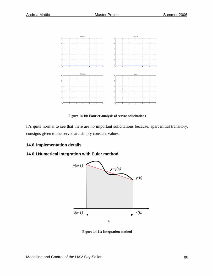
Andrea Mattio Master Project Summer 2006
Modelling and Control of the UAV Sky-Sailor
80
Figure 14.10: Fourier analysis of servos-solicitations
It’s quite normal to see that there are no important solicitations because, apart initial transitory,
consigns given to the servos are simply constant values.
14.6 Implementation details
14.6.1 Numerical Integration with Euler method
Figure 14.11: Integration method
y(k)
y(k-1)
h
y=f(x)
x(k-1) x(k)

Andrea Mattio Master Project Summer 2006
Modelling and Control of the UAV Sky-Sailor
81
The integral value of ∫ −
)(
)1()(
kx
kxxf can be approximated with the value of trapeze area (gray
area).
So:
( )2
)1()()()(
)1(hkykyxf
kx
kx⋅−+
=∫ − (14.20)
and
( )2
)()1()()1(
)(hkykyxf
kx
kx⋅++
=∫+
and ( )∫∫ +
⋅++=
+)(
0
)1(
0)(
2)()1()(
kxkx
xfhkykyxf
(14.21)
Exploiting the two relationships (14.20) and (14.21):
∫ ∫−
+⋅=)(
0
)1(
0
)()()(kx kx
xfhkyxf (14.22)
This last relationship is the one used to implement the control on the DSPIC.
14.6.2 Numerical interpolation
Figure 14.12: Numerical interpolation
Numerical interpolation is used in the implementation to smoothen the set point of the roll given
by the LLC to the HLC. In fact instead of given a step as consign to the LLC, it’s better to
exploit the fact that where we want to go is known in advance ( it means that at instant k-1 the
roll(k)
roll(k-1)
1sec
t(k-1) t(k)

Andrea Mattio Master Project Summer 2006
Modelling and Control of the UAV Sky-Sailor
82
consign value for the following instant k is known), linearly interpolating between the two
values.
Knowing that t(k)-t(k-1)=1sec and that during this second the LLC is executed 25 times, the set
point of the LLC will be equal to:
25)(
251)1()( hkrollhkrollhroll ⋅+⎟
⎠⎞
⎜⎝⎛ −⋅−= with 25,...,0=h (14.23)
14.6.3 Filter implementation Considering a filter with the following configuration:
( )( ) ( ) 111 −⋅−−
=za
azUzY (14.24)
( ) ( )( ) ( )zUazazY ⋅=⋅−−⋅ −111 (14.25)
It’s possible to pass in the time discrete domain obtaining:
( ) )()1(1)( kuakyaky ⋅=−⋅−− (14.26)
( ) )()1(1)( kuakyaky ⋅+−⋅−= (14.27)
14.6.4 LLC pseudo code Data checking
If (abs(roll) < 30° &
abs(pitch) < 30° &
7 m/s < wind speed < 15 m/s)
Data ok {
Angles Transformation between two different Tait-Bryant sequence roll_ctrl = asin(cos_pitch*sin_roll); pitch_ctrl = atan2(sin_pitch,cos_pitch*cos_roll); Determination of roll and pitch derivatives from angular rates values
droll_ctrl = cos_pitch_ctrl * gyrX
+sin_pitch_ctrl * gyrZ; dpitch_ctrl = sin_pitch_ctrl*sin_roll_ctrl/cos_roll_ctrl* gyrX + 1 * gyrY -cos_pitch_ctrl*sin_roll_ctrl/cos_roll_ctrl*gyrZ; Integration

Andrea Mattio Master Project Summer 2006
Modelling and Control of the UAV Sky-Sailor
83
int_roll_ctrl += (set_pt_roll - roll_ctrl) * 0.04; int_wind_speed_f += (set_pt_wind_speed_f - wind_speed_f) * 0.04; int_accY += accY * 0.04; Interpolation of roll set point
set_pt_roll = set_pt_roll_old * (1-Ctrl_25Hz_Timer/25)+ set_pt_roll_new * Ctrl_25Hz_Timer/25;
Eventual altitude saturation if (fabsf(set_pt_altitude - altitude_ctrl) > 0.2) if ( (set_pt_altitude - altitude_ctrl) < 0) altitude_sat = -0.2; else altitude_sat = 0.2; else altitude_sat = set_pt_altitude - altitude_ctrl; LQR implementation u_ail = K(1,:)*[control_states]’; u_vtail_l = K(1,:)*[control_states]’;
u_vtail_r = K(1,:)*[control_states]’; u_motor = K(1,:)*[control_states]’;
Filter on commands
actual_value = a*new_value + (1-a)*old_value); }
else Data KO { Commands set to neutral position u_ail_consign = u_ail_set_pt; u_vtail_l_consign = u_vtail_l_set_pt; u_vtail_r_consign = u_vtail_r_set_pt; u_motor_consign = 0; }
END
14.6.5 HLC pseudo code START Data reception
GPS
Data checking
If (GPS_data ok) Data OK
{ Circle trajectory generation freq = set_pt_wind_speed_f / (2*PI*radius);

Andrea Mattio Master Project Summer 2006
Modelling and Control of the UAV Sky-Sailor
84
sin_traj = sin(2*freq*PI*time); cos_traj = cos(2*freq*PI*time); x1 = radius*cos_traj; x1d = -2*freq*PI*radius*sin_traj; x1dd = -4*freq*freq*PI*PI*radius*cos_traj; x2 = radius*sin_traj; x2d = 2*freq*PI*radius*cos_traj; x2dd = -4*freq*freq*PI*PI*radius*sin_traj; Heading generator
chi1_kplus1 = (-k*k*k*int1 - 3*k*k*(latitude_rel_meter -x1) - 3*k*(chi1-x1d) + x1dd) * 1 + chi1;
chi2_kplus1 = (-k*k*k*int2 - 3*k*k*(longitude_rel_meter-x2) - 3*k*(chi2-x2d) + x2dd) * 1 + chi2;
int1_kplus1 = (latitude- x1) * 1 + int1; int2_kplus1 = (longitude-x2) * 1 + int2; x3_hat = atan2(chi2,chi1); int1 = int1_kplus1; int2 = int2_kplus1; chi1 = chi1_kplus1; chi2 = chi2_kplus1;
last_errx3 = errx3; errx3 = atan2(sin(x3_hat-heading_gps),cos(x3_hat-heading_gps)); PI control
set_pt_roll_old = set_pt_roll_new; set_pt_roll_new = 0.2 * errx3 - 0.19 * last_errx3 + set_pt_roll_new; }
Data KO
Set_pt_roll_new = 4°
END
14.7 Fourier Transformation and Power Spectral Density To analyze servos solicitations Fourier analysis has been used. In particular MatLab fft(Fast
Fourier Transformation) and the concept of Power Spectral Density. Fourier Transformation evaluation FFT_ail_out = fft(u_ail_out - mean(u_ail_out)); freq = (1/0.04)*[0:length(u_ail_out)/2]/length(u_ail_out); Power Spectral Density evaluation PP_ail_out = FFT_ail_out.*conj(FFT_ail_out);

Andrea Mattio Master Project Summer 2006
Modelling and Control of the UAV Sky-Sailor
85
14.8 dsPIC general features dsPIC is a family of microcontrollers that joins the structure of a microcontroller with the that of
a DSP (Digital Signal Processor). This family is made up of three other families:
• General purpose family ( codec interface)
• Sensor family (small ones)
• Motor control family ( with PWM control and encoder)
Figure 14.13: General structure of dsPIC

Andrea Mattio Master Project Summer 2006
Modelling and Control of the UAV Sky-Sailor
86
Figure 14.14: dsPIC structure
Structure heart Addresses
BUS x and y Peripherals

Andrea Mattio Master Project Summer 2006
Modelling and Control of the UAV Sky-Sailor
87
14.9 Bus I2C The bus I2C is simple bidirectional 2-wire bus for efficient inter-IC control.
The I2C bus physically consists of 2 active wires and a ground connection. The active wires,
called SDA and SCL, are both bi-directional. SDA is the Serial Data line, and SCL is the Serial
Clock line.
Every device hooked up to the bus has its own unique address, no matter whether it is an MCU,
LCD driver, memory, or ASIC. Each of these chips can act as a receiver and/or transmitter,
depending on the functionality. Obviously, an LCD driver is only a receiver, while a memory or
I/O chip can be both transmitter and receiver.
The I2C bus is a multi-master bus. This means that more than one IC capable of initiating a data
transfer can be connected to it. The I2C protocol specification states that the IC that initiates a
data transfer on the bus is considered the Bus Master. Consequently, at that time, all the other
ICs are regarded to be Bus Slaves.
As bus masters are generally microcontrollers, let's take a look at a general 'inter-IC chat' on the
bus. Let consider the following setup and assume the MCU wants to send data to one of its
slaves.
Figure 14.15: I2C scheme
First, the MCU will issue a start condition. This acts as an 'Attention' signal to all of the
connected devices. All ICs on the bus will listen to the bus for incoming data.
Then the MCU sends the address of the device it wants to access, along with an indication
whether the access is a Read or Write operation (Write in our example). Having received the
address, all IC's will compare it with their own address. If it doesn't match, they simply wait
until the bus is released by the stop condition (see below). If the address matches, however, the
chip will produce a response called the acknowledge signal.

Andrea Mattio Master Project Summer 2006
Modelling and Control of the UAV Sky-Sailor
88
Once the MCU receives the acknowledge, it can start transmitting or receiving DATA. In our
case, the MCU will transmit data. When all is done, the MCU will issue the stop condition. This
is a signal that the bus has been released and that the connected ICs may expect another
transmission to start any moment.
Start, address, acknowledge, data, stop are all unique conditions on the bus.