![Simulation Modelling Practice and Theory · A semi-active control of vehicle suspension system with magnetorheological (MR) damper has been presented by Yao et al. [13]. Spentzas](https://static.fdocuments.net/doc/165x107/5ede71fcad6a402d6669c444/simulation-modelling-practice-and-theory-a-semi-active-control-of-vehicle-suspension.jpg)
Modelling and Control of Magnetorheological Damper: Real ... · Modelling and Control of...
199
General rights Copyright and moral rights for the publications made accessible in the public portal are retained by the authors and/or other copyright owners and it is a condition of accessing publications that users recognise and abide by the legal requirements associated with these rights. Users may download and print one copy of any publication from the public portal for the purpose of private study or research. You may not further distribute the material or use it for any profit-making activity or commercial gain You may freely distribute the URL identifying the publication in the public portal If you believe that this document breaches copyright please contact us providing details, and we will remove access to the work immediately and investigate your claim. Downloaded from orbit.dtu.dk on: Jun 28, 2020 Modelling and Control of Magnetorheological Damper: Real-time implementation and experimental verification Bhowmik, Subrata Publication date: 2012 Document Version Publisher's PDF, also known as Version of record Link back to DTU Orbit Citation (APA): Bhowmik, S. (2012). Modelling and Control of Magnetorheological Damper: Real-time implementation and experimental verification. DTU Mechanical Engineering. DCAMM Special Report, No. S139
Transcript of Modelling and Control of Magnetorheological Damper: Real ... · Modelling and Control of...

General rights Copyright and moral rights for the publications made accessible in the public portal are retained by the authors and/or other copyright owners and it is a condition of accessing publications that users recognise and abide by the legal requirements associated with these rights.
Users may download and print one copy of any publication from the public portal for the purpose of private study or research.
You may not further distribute the material or use it for any profit-making activity or commercial gain
You may freely distribute the URL identifying the publication in the public portal If you believe that this document breaches copyright please contact us providing details, and we will remove access to the work immediately and investigate your claim.
Downloaded from orbit.dtu.dk on: Jun 28, 2020
Modelling and Control of Magnetorheological Damper: Real-time implementation andexperimental verification
Bhowmik, Subrata
Publication date:2012
Document VersionPublisher's PDF, also known as Version of record
Link back to DTU Orbit
Citation (APA):Bhowmik, S. (2012). Modelling and Control of Magnetorheological Damper: Real-time implementation andexperimental verification. DTU Mechanical Engineering. DCAMM Special Report, No. S139

Modelling and Control of Magnetorheological Damper:
Real-time implementation and experimental verifi cation
Ph
D T
he
sis
Subrata BhowmikDCAMM Special Repport No. S139October 2011


Modelling and Control
of Magnetorheological Damper:
Real time implementation
and experimental verification
Subrata Bhowmik
Department of Mechanical Engineering
Technical University of Denmark
Lyngby, Denmark
2011


Abstract
This thesis considers two main issues concerning the application of a rotary type magne-torheological (MR) damper for damping of flexible structures. The first is the modelling andidentification of the damper property, while the second is the formulation of effective controlstrategies. The MR damper is identified by both the standard parametric Bouc-Wen modeland the non-parametric neural network model from an experimental data set generated bydynamic tests of the MR damper mounted in a hydraulic testing machine. The forwardmodel represents the direct dynamics of the MR damper where velocity and current areused as input and the force as output. The inverse model represents the inverse dynamicsof the MR damper where the absolute velocity and absolute force are used as input and thedamper current as output. For the inverse model the current output of the network must al-ways be positive, and it is found that the modelling error of the inverse model is significantlyreduced when the corresponding input is given in terms of the absolute values of velocityand damper force. This is a new contribution to the inverse modelling techniques for thecontrol of MR dampers. Another new contribution to the modelling of an MR damper isthe use of experimental measurement data of a rotary MR damper that requires appropri-ate filtering. The semi-systematic optimisation procedure proposed in the thesis derives aneffective neural network structure, where only velocity and damper force are essential inputparameters for the MR damper modelling. Thus, for proper training, the quality of thevelocity data is very important. However, direct velocity measurement is not easy. Fromthe displacement data or the acceleration data, velocity can be determined by using simpledifferentiation or integration, respectively, but these processes add undesirable noise to thevelocity. Instead the Kinematic Kalman Filter (KKF) is an effective means for estimationof velocity. The KKF does not directly depend on the system or structural model, as itis the case for the conventional Kalman filter. The KKF fuses the displacement and theacceleration data to get an accurate and robust estimate of the velocity. The simplicity ofthe network and the application of velocity in terms of KKF is a novel contribution of thethesis to the generation of a training set for neural network modelling of MR dampers.
The development of the control strategies for the MR damper focuses on the introduction ofapparent negative stiffness, which basically leads to an increased local motion of the damperand thereby to increased energy dissipation and damping. Optimal viscous damping (VD)is chosen as the benchmark control strategy, used as reference case for assessment of theproposed control methods with negative stiffness. Viscous damping with negative stiffness(VDNS) initially illustrates the effectiveness of the negative stiffness component in struc-tural damping. In a linear control setting negative stiffness requires active control forces,which are not realizable by the purely dissipative MR damper. Thus, these active compo-nents are simply clipped in the final control implementation. Since MR dampers behavealmost as a friction damper improved damping performance can be obtained by a suitablecombination of pure friction and negative damper stiffness. This is realized by amplitudedependent friction damping with negative stiffness (FDNS), where the force level of thefriction component is adaptively changed to secure the optimal balance between friction en-ergy dissipation and apparent negative stiffness. This type of control model for semi-activedampers is rate-independent and conveniently described in terms of the desired shape of theassociated hysteresis loop or force-displacement trajectory. The final method considered forcontrol of the rotary MR damper is a model reference neural network controller (MRNNC).This novel control approach is designed and trained based on a desired reference dampermodel, which in this case is the amplitude dependent friction damping with negative stiffness(FDNS). The idea is to train the neural network of the controller by data derived explicitlyfrom the desired shape of the force-displacement loop at pure harmonic motion. In this
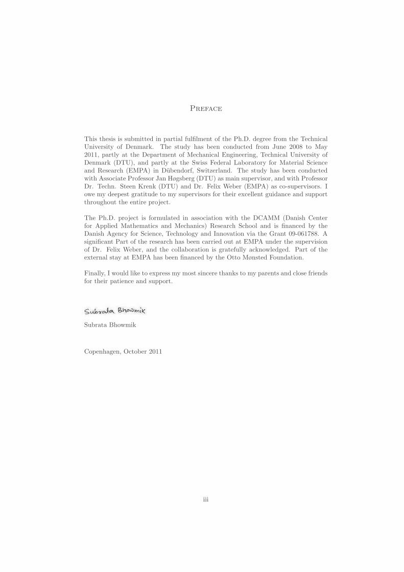
idealized representation the optimal relations between friction force level, negative stiffnessand response amplitude can often be given explicitly by e.g. maximizing the damping ratioof the targeted vibration mode. Consequently the idea behind this trained neural networkis that the optimal properties of the desired hysteresis loop formulation can be extrapolatedto more general and non-harmonic response patterns, e.g. narrow-band stochastic responsedue to wind, wave, traffic or even earthquake excitation.
Numerical and experimental simulations have been conducted to examine the performanceof the proposed control strategies. Force tracking by using an inverse neural network ofthe MR damper is improved by a low-pass filter to reduce the noise in the desired currentand a simple switch that truncates negative values of the desired current. The performanceof the collocated control schemes for the rotary type semi-active MR damper are initiallyverified by closed loop dynamic experiments conducted on a 5-storey shear frame structureexposed to harmonic base excitation. The MR damper is mounted on the structure so thatit operates on the relative motion between the ground base and the first floor of the shearframe. The shear frame structural model is initially experimentally identified, where massand stiffness of the model is determined by an inverse modal analysis based on the natu-ral frequencies obtained experimentally. The damping matrix is subsequently determinedfrom the estimated damping ratio obtained by free decay tests. The results in the thesisdemonstrate that introducing apparent negative stiffness to the control of the MR dampersignificantly decreases both the top floor displacement and acceleration amplitudes of theshear frame structure. The structural damping ratios obtained from the response curvesof the experiments correspond well to the expected values. This indicates that the meanstiffness and mean energy dissipation of the control forces are predicted fairly accurate.
A final numerical investigation is based on a classic benchmark problem for earthquakeprotection of a multi storey building. The seismic response of the base-isolated benchmarkbuilding with an MR damper installed between the ground and the base is illustrated, and theeffectiveness of negative stiffness of the control strategies is verified numerically. Similarly,the response of another wind excited benchmark building installed with MR dampers isdemonstrated and the performance shows satisfactory result.
The main contributions to this thesis are the novel modelling approach to the direct and theinverse dynamics of a rotary MR damper from experimental data, the development of modelbased semi-active control strategies for the MR damper, the effective introduction of negativestiffness in the control of semi-active dampers and the demonstration of effectiveness andclosed loop implementation of the control techniques on both a shear frame structure and anumerical benchmark problem.
ii
Preface
This thesis is submitted in partial fulfilment of the Ph.D. degree from the TechnicalUniversity of Denmark. The study has been conducted from June 2008 to May2011, partly at the Department of Mechanical Engineering, Technical University ofDenmark (DTU), and partly at the Swiss Federal Laboratory for Material Scienceand Research (EMPA) in Dubendorf, Switzerland. The study has been conductedwith Associate Professor Jan Høgsberg (DTU) as main supervisor, and with ProfessorDr. Techn. Steen Krenk (DTU) and Dr. Felix Weber (EMPA) as co-supervisors. Iowe my deepest gratitude to my supervisors for their excellent guidance and supportthroughout the entire project.
The Ph.D. project is formulated in association with the DCAMM (Danish Centerfor Applied Mathematics and Mechanics) Research School and is financed by theDanish Agency for Science, Technology and Innovation via the Grant 09-061788. Asignificant Part of the research has been carried out at EMPA under the supervisionof Dr. Felix Weber, and the collaboration is gratefully acknowledged. Part of theexternal stay at EMPA has been financed by the Otto Mønsted Foundation.
Finally, I would like to express my most sincere thanks to my parents and close friendsfor their patience and support.
Subrata Bhowmik
Copenhagen, October 2011
iii

Publications
Appended papers
[P1] S. Bhowmik, F. Weber, J. Høgsberg,
Experimental calibration of forward and inverse neural networks for rotary type magne-torheological damper,
(2011), Submitted for publication.
[P2] F. Weber, S. Bhowmik, J. Høgsberg,
Design and experimental verification of semi-active control with negative stiffness for MRdampers,
(2011), Submitted for publication.
[P3] S. Bhowmik,
Neural Network based semi-active control strategy for structural vibration mitigation withmagnetorheological damper,
COMPDYN 2011. Proceedings of the third ECCOMAS Thematic Conference on Computa-tional Methods in Structural Dynamics and Earthquake Engineering, 540–553,
May 25–28, Corfu, Greece, 2011.
[P4] S. Bhowmik, J. Høgsberg,
Semi-active control of magnetorheological dampers with negative stiffness,
SMART 09. Proceedings of the fourth ECCOMAS Thematic Conference on Smart Structuresand Materials, 581–590,
July 13–15, Porto, Portugal, 2009.
[P5] S. Bhowmik, J. Høgsberg, F. Weber,
Neural Network modeling of forward and inverse behavior of rotary MR damper,
NSCM-23. Proceedings of the Twenty Third Nordic Seminar on Computational Mechanics,169–172,
October 21–22, Stockholm, Sweden, 2010.
iv

Contents
1 Introduction 1
2 Modelling and Identification of a Rotary MR Damper 6
2.1 Experimental Setup . . . . . . . . . . . . . . . . . . . . . . . . . . . . . . . . 7
2.2 Parametric Model of the MR Damper: Simplified Bouc-Wen Model . . . . . . 9
2.3 Non-Parametric Neural Network Model of MR Damper . . . . . . . . . . . . 13
2.3.1 Post Processing of Measurement Data . . . . . . . . . . . . . . . . . . 15
2.3.2 Feedforward Backpropagation Neural Network Architecture . . . . . . 17
2.3.3 Neural Network Model Structure for MR Damper . . . . . . . . . . . 19
2.4 Model Validation . . . . . . . . . . . . . . . . . . . . . . . . . . . . . . . . . . 21
2.4.1 Forward MR Damper Model . . . . . . . . . . . . . . . . . . . . . . . 21
2.4.2 Inverse MR Damper Model . . . . . . . . . . . . . . . . . . . . . . . . 22
2.4.3 Emulation of Viscous Damping Using the Validated Model . . . . . . 22
2.5 Summary . . . . . . . . . . . . . . . . . . . . . . . . . . . . . . . . . . . . . . 24
3 Modelling of a Flexible Structure 30
3.1 Overview of Experimental Setup . . . . . . . . . . . . . . . . . . . . . . . . . 30
3.1.1 Measurement Sensors . . . . . . . . . . . . . . . . . . . . . . . . . . . 32
3.1.2 Hydraulic Actuators and Control Unit . . . . . . . . . . . . . . . . . . 32
3.1.3 Filtering . . . . . . . . . . . . . . . . . . . . . . . . . . . . . . . . . . . 33
3.2 Model Parameter Identification . . . . . . . . . . . . . . . . . . . . . . . . . . 34
3.2.1 Sine Sweep Test . . . . . . . . . . . . . . . . . . . . . . . . . . . . . . 35
3.2.2 Free Vibration Test . . . . . . . . . . . . . . . . . . . . . . . . . . . . 39
3.3 Equations of Motion . . . . . . . . . . . . . . . . . . . . . . . . . . . . . . . . 41
3.3.1 Mass Matrix . . . . . . . . . . . . . . . . . . . . . . . . . . . . . . . . 41
3.3.2 Stiffness Matrix . . . . . . . . . . . . . . . . . . . . . . . . . . . . . . . 41
3.3.3 Damping Matrix . . . . . . . . . . . . . . . . . . . . . . . . . . . . . . 42
3.3.4 Model Verification . . . . . . . . . . . . . . . . . . . . . . . . . . . . . 42
3.4 Summary . . . . . . . . . . . . . . . . . . . . . . . . . . . . . . . . . . . . . . 42
4 Control Strategies and Simulation 44
4.1 Damping of Flexible Structures . . . . . . . . . . . . . . . . . . . . . . . . . . 45
4.2 Two-Component System Reduction and Modal Damping . . . . . . . . . . . . 46
4.3 Control Strategies . . . . . . . . . . . . . . . . . . . . . . . . . . . . . . . . . 47
4.3.1 Optimal Viscous Damping . . . . . . . . . . . . . . . . . . . . . . . . . 48
4.3.2 Viscous Damping with Negative Stiffness . . . . . . . . . . . . . . . . 48
4.3.3 Amplitude Proportional Friction Damping with Negative Stiffness . . 49
v

4.3.4 Neural Network Based Model Reference Control . . . . . . . . . . . . 50
4.4 Closed-Loop Simulation . . . . . . . . . . . . . . . . . . . . . . . . . . . . . . 51
4.4.1 Example: Pure Viscous Damping . . . . . . . . . . . . . . . . . . . . . 51
4.4.2 Example: Viscous Damping with Negative Stiffness . . . . . . . . . . . 52
4.4.3 Example: Frictional Damping with Negative Stiffness . . . . . . . . . 52
4.4.4 Example: Neural Network based Model Reference Control . . . . . . . 54
4.5 Summary . . . . . . . . . . . . . . . . . . . . . . . . . . . . . . . . . . . . . . 57
5 Experimental Implementation of Control Strategies 58
5.1 Experimental Setup . . . . . . . . . . . . . . . . . . . . . . . . . . . . . . . . 58
5.2 Velocity Estimation Using Kinematic Kalman Filter . . . . . . . . . . . . . . 60
5.3 Closed-Loop Model Design in Matlab/Simulink . . . . . . . . . . . . . . . . . 60
5.4 Force Tracking . . . . . . . . . . . . . . . . . . . . . . . . . . . . . . . . . . . 62
5.5 Experimental and Numerical Simulation . . . . . . . . . . . . . . . . . . . . . 62
5.5.1 Pure Viscous Damping . . . . . . . . . . . . . . . . . . . . . . . . . . . 63
5.5.2 Viscous Damping with Positive Stiffness . . . . . . . . . . . . . . . . . 64
5.5.3 Viscous Damping with Negative Stiffness . . . . . . . . . . . . . . . . 65
5.5.4 Frictional Damping with Negative Stiffness . . . . . . . . . . . . . . . 66
5.6 Summary . . . . . . . . . . . . . . . . . . . . . . . . . . . . . . . . . . . . . . 68
6 Applications to Benchmark Problems 69
6.1 Magnetorheological Damper: Forward and Inverse Model . . . . . . . . . . . 70
6.2 Seismically Excited Base-Isolated Benchmark Building . . . . . . . . . . . . . 70
6.2.1 Structural Model and Evaluation Criteria . . . . . . . . . . . . . . . . 71
6.2.2 Numerical Simulation . . . . . . . . . . . . . . . . . . . . . . . . . . . 72
6.3 Wind-Excited Benchmark Building . . . . . . . . . . . . . . . . . . . . . . . . 76
6.3.1 Benchmark Structure . . . . . . . . . . . . . . . . . . . . . . . . . . . 76
6.3.2 Numerical Simulation . . . . . . . . . . . . . . . . . . . . . . . . . . . 77
6.4 Summary . . . . . . . . . . . . . . . . . . . . . . . . . . . . . . . . . . . . . . 79
7 Conclusions 80
Bibliography 82
A Base-Isolated Benchmark Model 89
B Evaluation Criteria For Base-Isolated Benchmark Building 93
C Wind-Excited Benchmark Model 95
D Evaluation Criteria For Wind-Excited Benchmark Building 96
E LQG Control Design: Sample Controller In Benchmark Problems 98
vi

Chapter 1
Introduction
Most flexible structures, such as high-rise buildings or bridges, have very little structuraldamping and are therefore often prone to dynamic excitation, e.g. from wind or seismicloading. Different control mechanisms are used to reduce structural fault and thus preventfailure.
Passive dampers are reliable in the sense that they rely purely on dissipation of incomingenergy without any power requirements. Some typical passive installations are tuned massdampers, see Rasouli et al. [1], or base-isolation systems, see Cho et al. [2] or referencesherein.
Fully active control systems are able to apply both dissipate and non-dissipative forces to thestructure, and when properly designed they yield a significant increase in damping comparedto passive dampers. However, active control typically requires a large amount of power andmay also introduce instabilities due to time delays or model uncertainties. Examples ofactive control systems are the active tuned mass dampers [1, 3] or tendon type control [4].As an alternative to the passive tuned mass dampers, an active tuned mass damper, wherean actuator is inserted between the structure and the secondary mass, can be considered asan effective damping device. The design of active tuned mass dampers is typically based onlinear quadratic regulator (LQR) theory. Preumont [4] developed and implemented velocityfeedback based active control strategies for civil structures. An active control strategy isdemonstrated in [5] for application to a flexible structure excited by simulated wind forcesfor the purpose of minimising along-wind accelerations. A linear quadratic Gaussian (LQG)control strategy based on acceleration feedback is used to reduce the structural responseeffectively. De and Zheng [6] also applied active control to a tall structure excited by windwhere a new active vibration control method which fits non-linear buildings is demonstrated.The control method is based on model identification and structural model linearisation andexerts the control force on the built model according to the force action principle.
Semi-active dampers are often considered to be a desirable compromise between failsafepassive damping and effective active control. They require little power for the operationand are thus able to run for instance on battery power. Besides, they do not add energyto the system, whereby the stability due to the damper is improved because control forcesare developed through proper adjustment of damping and stiffness components of controller.The most common types of semi-active dampers for civil engineering applications are variablestiffness dampers [7, 8] and magnetorheological (MR) dampers [9, 10]. A cylindrical typeMR damper designed and manufactured by Maurer Sohne GmbH is shown in Figure 1.1.
The characteristics of the MR damper are controlled in terms of the applied current, whichalmost simultaneously changes the magnetic field and thus the shear viscosity of the damper.A more detailed description of the characteristics and the modelling of MR dampers canbe found in for instance [11]. Semi-active MR dampers have been used for both dampingand earthquake protection of buildings, see e.g. [12, 13]. One of the most commonly usedcontrol strategies for MR dampers is the clipped-optimal control proposed by Dyke et al. [14].This algorithm consists of a bang-bang (on-off) type of controller that causes the damperto generate a desirable control force, determined by an optimal control algorithm, such as
1

2 Introduction
Figure 1.1: A Cylindrical Type Magnetorheological Damper (Courtesy of MaurerSohne GmbH).
the H2/LQG method. The optimal force is determined by using a full-order observer. Thisoptimal force is clipped by using the Heaviside function to get the desired voltage for the MRdamper to implement the semi-active control strategy on the MR damper. Zhu et al. [15]implemented a semi-active control strategy based on the linear quadratic Gaussian (LQG)method in a wind excited structure using the MR damper. Iemura et al. [16] presented bothpassive and semi-active control strategies for the MR damper for a stay cable bridge andshowed the effectiveness of semi-active control strategy over passive control strategy. Othercommon types of control strategies for MR dampers are based on e.g. Lyapunov functions,the bang-bang theory [10], variable friction damping strategy [17], modulated homogeneousfriction damping strategy [18] or sliding mode control [19, 20]. The Lyapunov stabilityanalysis is used for developing control laws where the goal is to choose control inputs foreach device that will result in making the derivative of the Lyapunov function as negative aspossible. The decentralised bang-bang theory is similar to the Lyapunov approach where theLyapunov function has been chosen to represent the total vibratory energy in the structure.A modulated homogeneous friction damping approach is proposed because there is strongsimilarities between the behaviour of a variable friction device and the MR damper [18]. Inthis control strategy, at each occurrence of a local maximum in the deformation of the device,the normal force applied to the frictional interface is updated to a new value. This methodis originally developed for friction dampers but it is modified for the MR damper based onMR damper properties. A detailed comparison of the most common control strategies forMR dampers can be found in [10].
Besides the above-mentioned classical control strategies, several intelligent control algo-rithms based on soft computing techniques are used for controlling the MR damper. Thesetechniques rely on proper training in the desired behaviour instead of accurate mathemat-ical models. Thus, they are suitable for solving and modelling of highly complex systems,such as damping of a flexible structure by control of a non-linear semi-active damper. Ex-amples of soft computing techniques for damping or control of structures are neural net-works [21, 22, 23, 24], fuzzy logic [25, 26], genetic algorithms [27] and various hybrid systems[27, 28].

3
In this thesis an MR damper in a collocated control setting is used to reduce the vibrationalresponse of a flexible structure, which is verified experimentally on a shear frame structureand numerically on benchmark problems. The effectiveness of negative stiffness in semi-active control design is demonstrated with different control strategies.
In this thesis four main objectives are considered. They are as follows:
� Development of semi-active control strategies for the MR damper.
� Modelling of direct and inverse dynamics of an MR damper and force tracking inclosed-loop simulation.
� Closed loop implementation of the semi-active control strategies.
� Implementation of the semi-active control strategies on benchmark problems.
The first part of the thesis presents a framework for design of external dampers for damp-ing of flexible structures. This is based on maximisation of the damping ratio of a criticalvibration form and it follows the two-component reduction technique presented by Mainand Krenk [29]. This analysis provides analytical expressions for the modal damping ratio,which indicates that effective damping can be obtained by imposing negative stiffness on thedamper. Four types of collocated control strategies are considered: (a) pure viscous damping,(b) viscous damping with negative stiffness, (c) amplitude dependent friction damping withnegative stiffness and (d) model reference neural controlling. In model reference neural con-trolling the reference model is considered as an optimal force-displacement hysteresis modelof a friction damper with negative stiffness. The shape is primarily identified by Boston etal. [30] by an evolutionary algorithm. The optimal force from the controller is then usedfor determining the desired current for the MR damper from the inverse MR model, whichis another task of the thesis and is discussed in the second part of the thesis. To improvethe performance of the controller, the stiffness parts are considered as negative. It has beendemonstrated by Iemura et al. [31] that optimal LQR control produces active damper forcesfor a structure with significant negative stiffness characteristics. In [32, 33] Iemura et al.further developed the strategy with pseudo negative stiffness dampers for seismically iso-lated structures and stay cables and demonstrated the effectiveness of negative stiffness bynumerical simulations. Moreover, for damping of stay cables Li et al. [34] demonstrated asignificant improvement due to the introduction of negative stiffness. Høgsberg [35] demon-strated the important role of negative stiffness in controlling of MR dampers for damping offlexible structures. Boston et al. [30] evaluated the optimal closed-form solution for frictiondamping with negative stiffness applying an MR damper to cable vibration and identified theoptimal shape of the force-displacement hysteresis loop. Very recently, Weber et al. [36, 37]demonstrated control strategies considering negative stiffness on cables with an MR damper.However, the efficiency of these techniques is still to be investigated numerically and exper-imentally by different optimal approaches on building structures because maximum workdone in earlier are mainly on benchmark building problem.
The second part of the thesis considers the realisation of the desired control force by anMR damper. The key to accurate tracking of the control force is a representative inversemodel of the MR damper, where the applied current is determined via knowledge of thedesired force. This part of the thesis presents a non-parametric modelling technique forneural network based system identification of the forward and inverse dynamics of the MRdamper. The real MR damper input-output data has been considered as training data foridentification of both the forward and the inverse model. The inverse feedforward neuralnetwork model is then used for force tracking for closed loop simulation.
The third part of the thesis presents closed loop implementation of the control strategiesby use of a rotary MR damper on a five-floor shear frame structure with harmonic base
4 Introduction
excitation. The shear frame structural model has been identified experimentally from a freedecay test and by modal analysis.
Further in this thesis, two numerical studies based on benchmark problems are presented.One of the numerical studies deals with the performance of the introduced semi-activecontrol schemes and is evaluated on the basis of the response of a base-isolated benchmarkstructure, introduced by Narasimhan et al. [38, 39], exposed to real earthquake record. Forthe second numerical study on benchmark problems, the evaluation is based on the responseof a 76-floor wind excited tall building introduced by Yang et al. [40]. This building hasbeen scaled and the scaled structure has been used in a wind tunnel test by Samali et al. [41]to generate along-wind and across-wind loading data. The control strategies are primarilybased on modal analysis where an approximate solution is obtained as an interpolationbetween the solutions of the two limiting eigenvalue problems: the undamped eigenvalueproblem and the constrained eigenvalue problem in which the MR damper is fully locked inits position. Optimal forces are evaluated for pure viscous, viscous with negative stiffnessand friction damping with negative stiffness. All of these control strategies are applied to aflexible structure by an MR damper.
The text is organised as follows. In Chapter 2, a systematic approach to the neural network(NN) modelling of both the forward and the inverse behaviour of a rotary MR damperis discussed. An optimisation procedure demonstrates that accurate training of the NNarchitecture for the forward damper model is obtained with velocity and current as inputstates. A similar architecture is then used to train the NN of the inverse MR damperbehaviour, but with the absolute values of velocity and force as input states to estimate thecurrent that is always a positive quantity. The forward and inverse models are validated byseveral measurements at different displacement frequencies and with different constants andhalf-sinusoidal current records. The validation shows satisfactory results for the forward aswell as the inverse model. The validated models are finally used to emulate pure viscousdamping. This simulation demonstrates that the main error of the inverse NN based modelis due to the modelling errors of the pre-yield behaviour of the MR damper.
Chapter 3 describes an experimental study to determine the system model parameters fromtest data. The experimental tests were performed using a shaking table. A five-mass shearframe structure has been used for model identification and it is excited by ground accelerationby the shaker. It is assumed that all the mass of the floor is lumped at the center of eachfloor. The stiffness of the model is determined from the mode shape which is constructedfrom the frequency transfer function from test data. The damping matrix is determined fromthe estimated damping ratio from a free decay test. This five-degree-of-freedom structurepossesses five natural frequencies corresponding to the number of degrees of freedom. Whenthe structure is subjected to the excitation, resonance is induced if the frequency of excitationis close to each of one of the natural frequencies of the structure. From the frequency responsethe resonance frequencies are determined. Validation of the model parameters is carried outby independent data sets and shows satisfactory results.
Collocated control strategies for a base excited shear frame building, where a single magne-torheological (MR) damper has been placed between ground and first floor are initially givenin Chapter 4. The calibration of the desired damper force is based on maximisation of thedamping ratio of the first vibration mode, and the associated damper current is determinedby an inverse MR damper. Four types of collocated control strategies are considered: (a)pure viscous damping, (b) viscous damping with negative stiffness, (c) amplitude dependentfriction damping with negative stiffness and (d) model reference neural controlling, whichmimics the behaviour of friction damping with negative stiffness. For the last three models,the desired stiffness is considered as negative, apparently softening the structure in the loca-tion of the damper, so that the damping of the structure is increased while the transmissionof the base excitation to the structure is potentially reduced. The closed-loop simulation is
5
discussed in detail.
In Chapter 5, closed loop implementation of control laws for vibration mitigation of the baseexcited five-floor building using a rotary MR damper is discussed. The experimental testsare performed using a shaking table and it is excited by harmonic base acceleration usinga shaker. The MR damper is located in between ground and first floor. The inverse MRmodel is designed on the basis of the velocity of the damper and, moreover, some control lawsare dependent on the velocity. Therefore, correct velocity estimation from displacement oracceleration data is very important. The Kinematic Kalman Filter (KKF) is used to estimatethe velocity of the damper by fusing displacement and acceleration. A detailed descriptionof the experimental setup and a comparison of the results are presented.
The numerical studies on the implementation of control strategies for vibration reduction fortwo benchmark problems are discussed in Chapter 6. Both the numerical study deals withthe performance of the introduced semi-active control schemes. The first numerical studyis evaluated on the basis of the response of a base-isolated benchmark structure exposedto real earthquake record and the second numerical study is evaluated on the basis of theresponse of a wind excited 76 floor tall building.
In Chapter 7, the conclusions of the presented work are summarised.

Chapter 2
Modelling and Identification of a Rotary MR Damper
Magnetorheological (MR) dampers used for controlled damping of structural vibrations havebeen given considerable attention during the last decades because they offer a possibilityof adapting their semi-active force in real-time to the structural vibrations [42]– [45]. MRdampers are suitable for mitigation of vibrations in large civil engineering structures becausethey combine large control force ranges, low-power requirements, fast response time andfailsafe performance [9]. MR dampers are either operated at zero or constant current,which is called passive-off and passive-on strategies [46] or they are controlled in real-time within a particular feedback loop [46, 47]. In the latter case the structural responseis typically measured in the damper position and the MR damper current is controlledin real-time for minimum tracking error with respect to the desired control force. Theforce tracking task is usually solved by a feedforward model in order to avoid costly forcesensors [46, 47, 48] in the real-time implementation. The inputs of the feedforward modelare the actual collocated displacement, velocity or acceleration, or any combination of thesestates, and the actual desired control force. The output is the actual desired current. Thisfeedforward model is also called the inverse model of the MR damper. The desired currentis tracked by a current driver that compensates for the coil impedance of the MR damper.Therefore, an MR damper model is required with damper force, displacement, velocityor acceleration as possible input states and the damper current as model output. Theforward model of the damper represents the damper itself, while the inverse model is usedfor e.g. tracking of a desired damper force in closed loop control. Many parametric andnon-parametric forward models have been presented in the literature for MR dampers of theclassical cylindrical type. Some of the prominent parametric approaches are the Bouc-Wenmodel, which captures both the pre- and post-yield regions [49, 50], the Dahl model, whichbasically represents current dependent friction [51, 52], the Bingham model, which describesan elasto-plastic material behaviour with supplemental viscous effects [53] and the LuGreapproach, which models the MR fluid particle chains as brushes with sticking and slidingeffects against the damper housing [54, 55, 56]. These models have also been extended byadditional stiffness, viscous and mass elements to account for the accumulator behaviour, thecurrent dependent viscous force and the inertia of the damper piston and other acceleratedparts [57, 58]. The parameters for minimum model error are typically obtained from thetest data directly [59, 60] or by a numeric optimisation tool [61, 62, 63]. Once calibrated,these parametric approaches can be used as observers to solve the force tracking problemwithout feedback from a force sensor [48].
Non-parametric models are mainly based on fitted polynomials [47], genetic algorithms [64],fuzzy logic [65], neural networks [66]– [72] or hybrid approaches [73]. As demonstratedin [66] the neural network approach is able to model the forward MR damper behaviourfairly accurately. Most of the neural networks are trained with simulated input-outputdata, usually generated by the Bouc-Wen model, as e.g. in [68]. Few neural networks havebeen trained with measured data [72], containing system noise and knocking effects due tobearing tolerances. This makes the training of the network much more difficult. The neuralnetwork architecture is usually found by a trial and error method, and the resulting neuralnetwork architecture is therefore not necessarily optimal with respect to the minimisation
6

2.1 Experimental Setup 7
of the modelling error.
The present chapter provides a systematic approach to the design and calibration of neuralnetworks of the forward and inverse behaviour of a rotary type MR damper based on mea-sured data. The MR damper behaviour is measured at constant and half-sinusoidal current.The half-sinusoidal current tests are performed because they generate training data verysimilar to the current records associated with emulated viscous damping. In the first partof this chapter a parametric modified Bouc-Wen model of the rotary type MR damper isdeveloped from experimental data sets. The original Bouc-Wen model has been modified tocapture the important characteristics of the MR damper behaviour. But the parametric ap-proach is only suitable to model the forward dynamics of the MR damper, while the inversedynamics are difficult to obtain and model because of the complicated and highly non-linearproperties of the MR damper model. The chapter further on describes a semi-systematicapproach to a suboptimal neural network architecture for finding the minimum modellingerror. The architecture of the neural networks for both the forward and the inverse MRdamper models is presented. The forward and inverse models are validated by measurementdata that is independent of the training data, and good accuracy is reported. Finally, thevalidated inverse and forward models are used in numerical simulations, where pure viscousdamping is reproduced in real-time. The detailed methodologies about forward and inverseMR damper modeling using neural network are also discussed in [P1, P5].
2.1 Experimental Setup
The MR damper considered is an MR damper of the rotary type manufactured by MaurerSohne GmbH with a maximum current limit of 4 A. The damper is shown in Figure 2.1with the hydraulic test set up. The rotary type MR damper consists of a housing includingthe MR fluid and the rotating part of the disc. The MR fluid is a suspension of oil withmagnetizable particles with average diameter of 5 μm and some additives. The particlesand the ferromagnetic parts of the housing and of the disc are magnetized by the magneticfield that is produced by two coils which are installed within the housing at both sides ofthe disc. The magnetized particles built chains and stick to the disc and to the housingWhen the disc starts to rotate the particle chains are initially stretched before they startto slide relative to the surfaces of the disc and/or the housing. The particle chains mayalso break, whereby rupture between particles occurs. The phase where particle chains areelastically stretched is commonly denoted as the pre-yield region of the MR fluid, while thesliding phase is called the post-yield region. The particle chains start to slide when the dryfriction force between particles or between particle chains and disc or housing is balancedby the elastic force due to elongation of the particle chains. Since this sticking dependsstrongly on the magnetization of the MR fluid, and thereby on the MR damper current, thepost-yield force of the MR damper typically exhibits a strong current dependency. Becausethe superposed viscous force is usually rather small and the MR fluid viscosity depends onlyslightly on the coil current, the applied current primarily controls the friction force of theMR damper, while the viscous force component is mainly governed by the rotating speed ofthe disc and the inherent viscosity of the MR fluid. In order to be able to control the totalMR damper force relative to a desired control force, the coil current must be modulated sothat the control force tracking error is acceptable. Due to the non-linear beaviour of theMR damper force, i.e. the non-linear relation between current and sticking force and thenon-linear current dependency of the MR fluid viscosity, feedback control only with a forcesensor may fail to track the desired force accurately. Figure 2.2(a) shows a close-up of thedamper of the rotary type at the Swiss Federal Laboratory of Material Science and Research(EMPA) and the schematic diagram of the damper is shown in Figure 2.2(b). Further detailson the damper characteristics can be found in [48, 60] and also in [P1]. The damper forceis slightly velocity dependent and the force level is approximately 30 N at 0 A and 300 N

8 Modelling and Identification of a Rotary MR Damper
Figure 2.1: Hydraulic test set-up with rotary MR damper.
at 4 A. The training and the validation data is obtained from forced displacement testsusing a hydraulic testing machine of the INSTRON type, see Figure 2.1. The desired pistondisplacement is defined in Matlab/dSPACE that outputs the displacement command signalto the INSTRON PC unit. A flow diagram of the experimental setup is shown in Figure 2.3.
The actual displacement is captured directly as output from the INSTRON machine andacquired by the dSPACE system at a sampling frequency of 1000 Hz. The sampling frequencyfor the force and acceleration measurements are 1000 Hz. The desired MR damper currentis also defined in Matlab/dSPACE. The output, i.e. desired current, is tracked using a
MR fluid
steel disc
metallic housing
coil
Figure 2.2: Rotary MR damper (a) and Schematic view of the damper (b)

2.2 Parametric Model of the MR Damper: Simplified Bouc-Wen Model 9
Figure 2.3: Schematic of test set-up.
current driver of the KEPCO type. The actual damper current is measured by the KEPCOamplifier and acquired by the dSPACE system. The MR damper force is measured by a500 N load cell manufactured by PCM, and the acceleration of the piston is also measuredin order to use it later, if required, as training data. Furthermore, the acceleration issuitable for detection of the knocking effects due to the finite bearing tolerances of 0.01-0.02mm of the joints of the damper rod. A summary of the tests conducted is provided inTable 2.1. Each test is performed twice: The first set is used as training data, while thesecond completely independent set is used to validate the neural network models. Tests 1-10are performed at constant current, while tests 11-19 are conducted at half-sinusoidal current,which is the mathematically absolute value of current. As seen in Table 2.1 the desireddisplacement is pure sinusoidal, combining amplitudes of 5 mm and 10 mm, and frequenciesrange from 0.5 Hz to 2.2 Hz [P1]. The training set and validation data set are separatedeach other by combining different displacement and current with different amplitude anddifferent frequency. The table only showing some data example. This amplitude rangeof displacement is based on practical information about the structure which is used forimplementing control strategies. The amplitude range contains the maximum amplitudewhich the structure can sustain before collapse. Moreover, in the frequency range the firstresonance frequency of the structure is contained.
2.2 Parametric Model of the MR Damper: Simplified Bouc-Wen Model
The rotational MR damper is modelled using the simplified Bouc-Wen hysteresis model.The parameters of the model have been calibrated from data sets generated by experiments,where the damper has been driven harmonically in a testing machine at various frequency-amplitude combinations of current and displacement. The modified Bouc-Wen model bySpencer et al. [11] was formulated for the cylindrical type MR damper. In the present casethis model is slightly simplified, mainly because the cylindrical damper concept has no needfor an accumulator chamber, which for many dampers of the cylindrical type introducesan additional stiffness component in the mathematical model. A schematic diagram of the

10 Modelling and Identification of a Rotary MR Damper
Table 2.1: Measurement data for training of NN and model validation.
train-ingset
vali-dationset
desired displacement desired current
1a 1b sine, 5 mm, [0.5, 1.0, 1.27, 1.8, 2.2] Hz 0 A
2a 2b sine, 5 mm, [0.5, 1.0, 1.27, 1.8, 2.2] Hz 1 A
3a 3b sine, 5 mm, [0.5, 1.0, 1.27, 1.8, 2.2] Hz 2 A
4a 4b sine, 5 mm, [0.5, 1.0, 1.27, 1.8, 2.2] Hz 3 A
5a 5b sine, 5 mm, [0.5, 1.0, 1.27, 1.8, 2.2] Hz 4 A
6a 6b sine, 10 mm, [0.5, 1.0, 1.27, 1.8, 2.2] Hz 0 A
7a 7b sine, 10 mm, [0.5, 1.0, 1.27, 1.8, 2.2] Hz 1 A
8a 8b sine, 10 mm, [0.5, 1.0, 1.27, 1.8, 2.2] Hz 2 A
9a 9b sine, 10 mm, [0.5, 1.0, 1.27, 1.8, 2.2] Hz 3 A
10a 10b sine, 10 mm, [0.5, 1.0, 1.27, 1.8, 2.2] Hz 4 A
11a 11b sine, 5 mm, [0.5, 1.0, 1.27, 1.8, 2.2] Hz half-sin, 0 A, [0.5, 1.0, 1.27, 1.8, 2.2] Hz
12a 12b sine, 5 mm, [0.5, 1.0, 1.27, 1.8, 2.2] Hz half-sin, 1 A, [0.5, 1.0, 1.27, 1.8, 2.2] Hz
13a 13b sine, 5 mm, [0.5, 1.0, 1.27, 1.8, 2.2] Hz half-sin, 2 A, [0.5, 1.0, 1.27, 1.8, 2.2] Hz
14a 14b sine, 5 mm, [0.5, 1.0, 1.27, 1.8, 2.2] Hz half-sin, 3 A, [0.5, 1.0, 1.27, 1.8, 2.2] Hz
15a 15b sine, 5 mm, [0.5, 1.0, 1.27, 1.8, 2.2] Hz half-sin, 4 A, [0.5, 1.0, 1.27, 1.8, 2.2] Hz
16a 16b sine, 10 mm, [0.5, 1.0, 1.27, 1.8, 2.2] Hz half-sin, 1 A, [0.5, 1.0, 1.27, 1.8, 2.2] Hz
17a 17b sine, 10 mm, [0.5, 1.0, 1.27, 1.8, 2.2] Hz half-sin, 2 A, [0.5, 1.0, 1.27, 1.8, 2.2] Hz
18a 18b sine, 10 mm, [0.5, 1.0, 1.27, 1.8, 2.2] Hz half-sin, 3 A, [0.5, 1.0, 1.27, 1.8, 2.2] Hz
19a 19b sine, 10 mm, [0.5, 1.0, 1.27, 1.8, 2.2] Hz half-sin, 4 A, [0.5, 1.0, 1.27, 1.8, 2.2] Hz
Bouc-Wen
Co
x
F
Figure 2.4: Bouc-Wen model of MR damper
simplified Bouc-Wen model is shown in Figure 2.4.
The governing equations for the damper force f predicted by the present Bouc-Wen modelcan be written as follows:
f = αz + c0x (2.1)
where the hysteresis effect follows from the evolutionary variable z controlled by the Bouc-

2.2 Parametric Model of the MR Damper: Simplified Bouc-Wen Model 11
Table 2.2: MR damper parameters
αa 4.038 N/m η 100 s−1
αb 1.984 N/m γ 410 s−2
αc 7.901 N/m β 410 s−2
αd -0.704 N/m A 1000
c0a 10 Ns/m c0b 100 Ns/m
Wen equationz = −γ|x|z|z|n−1 − βx|z|n +Ax (2.2)
The gain parameters on the hysteresis effect and the viscous effect are in the present casedescribed by cubic and linear functions of the applied current, respectively:
α = αa + αbu+ αcu2 + αdu
3 , c0 = c0a + c0bu (2.3)
The dynamics involved in the MR fluid reaching equilibrium state is represented throughfirst order filter. The applied current u is described with a time delay relative to the desiredcurrent I by the following first order filter:
u = −η(u− I) (2.4)
A Nelder-Mead direct search simplex method based on multidimensional unconstrained non-linear optimization is available by the standard MATLAB function fminsearch. It is used toestimate the parameters of the modified Bouc-Wen model by minimizing a scalar quadraticcost function of the system variables of the model. It is turns out this is a simple and effectivederivative free optimization method. The objective function used for minimization in thedirect search method is the RMS value of error between the measured and predicted forcevalues. The parameters of the rotary type MR dampers are derived from measurement datafrom the real MR damper. Maximum number of iteration is 1000 and the minimum erroris 0.01. Convergence is an important issue for this algorithm. Sometimes this algorithmconverge on non-stationary point instead of stationary point.This can be solved by restartthe algorithm with the final point as the new initial guess. The flow chart for the parametricidentification method of rotary type MR damper from experimental data is shown in Fig-ure 2.5. The estimated parameters of the simplified Bouc-Wen model for the rotational MRdamper are given in Table 2.2. The value of n is 2.
Typical force-displacement and force-velocity hysteresis loops for the rotational MR damperat different constant current are shown in Figure 2.6. It is visible that the MR damperbehaves approximately as a friction damper where the friction force level can be altered bychanging the applied damper current. The opening of the force-velocity loops indicates somepre-yield stiffness. The predicted force and the measured force value are compared in timedomain. The force-displacement hysteresis diagram for measurement data and predicteddata from the Bouc-Wen model are compared. In Figure 2.7(a,c), the comparisons of themeasured force data and the predicted force data from the model at constant current 0 A andsinusoidal displacement of 5 mm at two different frequency 0.5 Hz and 1.0 Hz are illustrated.The comparision between force-displacement trajectories for measured and predicted forcedata at constant current 0 A and sinusoidal displacement of 5 mm at two different frequency0.5 Hz and 1.0 Hz are also shown in Figure 2.7(b,d). The model validations in time domainand force-displacement trajectories for constant current 2 A and sinusoidal displacement 5mm, 1.0 Hz are shown in Figure 2.8(a,b)and for sinusoidal current 4 A, 2.0 Hz and sinusoidaldisplacement 5 mm, 2.0 Hz are shown in Figure 2.8(c,d). The model validations in time

12 Modelling and Identification of a Rotary MR Damper
Load test datadisplacement (x), current (I),
acceleration (x),force (f )m
Calculate Velocity (x)
from x and x
...
..
Set initial model parameter
value
Calculate predicted force (f)
Minimize objective functionJ = RMS (Err)
using “fminsearch’’
where Err = f-f
yes
m
End
update model parameter
No
Figure 2.5: Parametric identification flow chart.
domain and force-displacement trajectories for sinusoidal current 1 A, 1.0 Hz and sinusoidaldisplacement 5 mm, 1.0 Hz are shown in Figure 2.9(a,b) and for sinusoidal current 3 A, 1.0Hz and sinusoidal displacement 5 mm, 1.0 Hz are shown in Figure 2.9(c,d). The measuredand predicted forces from model are quite identical, but the Bouc-Wen model has significantlimitation in the post yield region because the real rotary damper has high nonlinearity inpost yield region which is not properly described by Bouc-Wen model. It is also visible in
−0.015−0.01−0.005 0 0.005 0.01−400
−200
0
200
400
Force,N
Displacement, m
4A
3A
2A1A0A
−0.2 −0.1 0 0.1 0.2−400
−200
0
200
400
Force,N
Velocity, m/s
4A
3A
2A1A
0A
Figure 2.6: Force-Displacement (a) Force-Velocity hysteresis loop (b)

2.3 Non-Parametric Neural Network Model of MR Damper 13
0 2 4 6 8 10−50
0
50measuredmodel
Force,
N
Time, s
(a)−6 −4 −2 0 2 4 6
x 10−3
−50
0
50measuredmodel
Force,
N
Displacement, m
(b)
0 2 4 6 8 10−50
0
50measuredmodel
Force,
N
Time, s
(c)−6 −4 −2 0 2 4 6
x 10−3
−50
0
50measuredmodel
Force,
NDisplacement, m
(d)
Figure 2.7: Model validation at current 0 A, displacement 5 mm, 0.5 Hz (a,b),Model validation at current 0 A, displacement 5 mm, 1.0 Hz (c,d)
the above mentioned figures that there is certain asymmetry in the hysteresis loops of theMR damper obtained from the measurement data. This asymmetry is mainly due to the so-called stribeck effect, which occurs between the pre- and post-yield regions. It is one of theimportant issues concerning the accurate modelling of rotary type MR dampers. Figure 2.7shows the damper response at zero current and fairly slow motion with frequencies of 0.5Hzand 1.0Hz. In Figure 2.8 the current is increased to 2A and 4A, while the frequency is alsoincreased slightly. Furthermore, the 4A case is for sinusoidal current with frequency 2.0Hz.Thus, this figure shows the effect of non-constant damper current, and the difference to thepassive case is clearly observed. In Figure 2.9 the current is also sinusoidal at low amps andslow motion. In that case the deviation from typical passive behaviour is not as significant.Pinching effect is visible in MR damper hysteresis diagram and this is mainly due to MRfluid flow constriction between disc and the metallic housing in rotational MR damper. Thepreliminary results for the Bouc-Wen model in Figures 2.7-2.9 show that the rotary MRdamper can be represented by the parametric Bouc-Wen model, but due to some limitationsit has difficulties representing some of the highly non-linear effects. For this reason thenon-parametric approach based on neural network modelling is adopted for a proper andaccurate modelling of both the forward and inverse MR damper dynamics.
2.3 Non-Parametric Neural Network Model of MR Damper
This section describes the post processing of the measurement data and the training of theneural network. Section 2.3.1 describes the filtering of the measurement data and how thesingle test series are combined to get a full training data time history. In Section 2.3.2 theneural network architecture is optimised, while Subsection 2.3.3 presents the identified neuralnetwork models used to model both the forward and the inverse MR damper characteristics.

14 Modelling and Identification of a Rotary MR Damper
0 2 4 6 8 10
−50
0
50measuredmodel
Force,
N
Time, S
(a)
−6 −4 −2 0 2 4 6
x 10−3
−50
0
50measuredmodel
Force,
N
Displacement, m
(b)
0 0.5 1 1.5 2
−300
−200
−100
0
100
200
300 measuredmodel
Force,
N
Time, S
(c)
−6 −4 −2 0 2 4 6
x 10−3
−300
−200
−100
0
100
200
300 measuredmodel
Force,
N
Displacement, m
(d)
Figure 2.8: Model validation at current 2 A, displacement 5 mm, 1.0 Hz (a,b),Model validation at current sin 4 A, 2.0 Hz displacement 5 mm, 2.0 Hz (c,d)
0 1 2 3 4 5
−50
0
50measuredmodel
Force,
N
Time, S
(a)−6 −4 −2 0 2 4 6
x 10−3
−50
0
50measuredmodel
Force,
N
Displacement, m
(b)
0 2 4 6 8 10
−200
−100
0
100
200measuredmodel
Force,
N
Time, S
(c)
−6 −4 −2 0 2 4 6
x 10−3
−200
−100
0
100
200measuredmodel
Force,
N
Displacement, m
(d)
Figure 2.9: Model validation at current sin 1 A, 1.0 Hz displacement 5 mm, 1.0 Hz(a,b), Model validation at current sin 3 A, 1.0 Hz displacement 5 mm, 1.0 Hz (c,d)

2.3 Non-Parametric Neural Network Model of MR Damper 15
53.4 53.42 53.44 53.46 53.48 53.5−6
−4
−2
0
2
4
6
accele
ration [m
/s2]
disp.: sin, 5mm, 1.27Hz; current: 4A
time [s]
filtered &
offset removed
83.2 83.22 83.24 83.26 83.28 83.39.8
10
10.2
dis
pla
cem
ent [m
m]
disp.: sin, 10mm, 1.0Hz; current: 4A
10.1
9.9
filtered &
offset
removed
(a) (b)
time [s]
18.44 18.48 18.52 18.56 18.62.92
2.94
2.96
2.98
3
curr
ent [A
]
disp.: sin, 5mm, 0.5Hz; current: half-sin, 3A, 0.5Hz
(c) (d)
filtered
3.02
time [s]55.1 55.2 55.3 55.4 55.5 55.6 55.7
−80
−60
−40
−20
0
20
40
60
80
forc
e [N
]
disp.: sin, 5mm, 2.2Hz; current: half-sin 3A, 2.2Hz
unfiltered
filtered & offset removed
filtered & offset removedacceleration*100 [m/s2]
time [s]
knocking due to
bearing tolerance
visible in acceleration
unfiltered
unfiltered
unfiltered
Figure 2.10: Filtering of measurement data.
2.3.1 Post Processing of Measurement Data
The measurement data from the rotary MR damper from the test setup contains noise andhas also some offset. The measurement data is initially passed through a low-pass filter inorder to avoid that the neural network is trained by high-frequency signal components, e.g.due to noise and knocking effects [P1]. These types of external effects typically result in anincreasing modelling error in the neural network models. The applied low-pass filter has thefollowing properties:
� Digital Butterworth low-pass filter: It is very efficient for removing high-frequencynoise from measurement data.
� Filter order 2: The filter order is kept low so that the main shape and the peak valuesof the measurement data are not altered.
� Cutoff frequency 100 Hz: The cutoff value is kept higher to remove the high-frequencynoise from the measurement data without losing its proper shape.
Any offset in the displacement, acceleration and force signals is removed by simply balanc-ing of positive and negative maxima under steady state conditions. Another possibility ofremoving offset is a high-pass filter. But in the present case the simple adjustment via thesequence of minima and maxima effectively removes the offset. The effect of the filtering ofdisplacement, acceleration, damper current and the damper force is shown in Figure 2.10.For the displacement and the damper current the high-frequency dithers are carefully re-moved by the low-pass filter, and the main task is basically to avoid a too significant changein the phase and a reduction in the peak values. This is shown in Figure 2.10(a), where
16 Modelling and Identification of a Rotary MR Damper
the displacement amplitude is 10mm and the frequency is 1.0Hz, and in Figure 2.10(c),where the damper current is half-sinusoidal with an amplitude of 3A. The accelerationmeasurements are very sensitive to the various sources of noise, and the influence of thefilter therefore becomes evident in Figure 2.10(b). Figure 2.10(d) shows the damper force,where the main modification is the removal of the offset level. Note that the constant forcelevel at zero crossing is due to the previously mentioned knocking because of finite bearingtolerances. The effect is mainly visible in the acceleration signal, which is also shown inFigure 2.10(d). This effect has a significant influence on the neural network modelling, anda proper filtering is therefore important [P1].
0 100 200 300 400 500 600 700 800 900
0
2
4
6
8
10
12
const.
const.
const.
const.
const.
ha
lf-s
in
ha
lf-s
in
ha
lf-s
in
ha
lf-s
in
ha
lf-s
in
[0.5,1.0,1.27,1.8,2.2] Hz
amplitude of desireddisplacement [mm]amplitude of desiredcurrent [A]
time [s]32.4 32.6 32.8 33 33.2 33.4 33.6
-0.04
-0.03
-0.02
-0.01
0
0.01
0.02
0.03
0.04
estim
ate
d v
elo
city [m
/s]
disp.: sin, 5mm, 1.0Hz; current: 4A
unfiltered
placement*5 [m]
2*pi*1Hz*0.005mm = 0.0314m/s
low pass filtered
filtered & offset
time [s]
(a) (b)
removed dis-
at 20Hz
Figure 2.11: Estimated velocity (a) and training data time history (b).
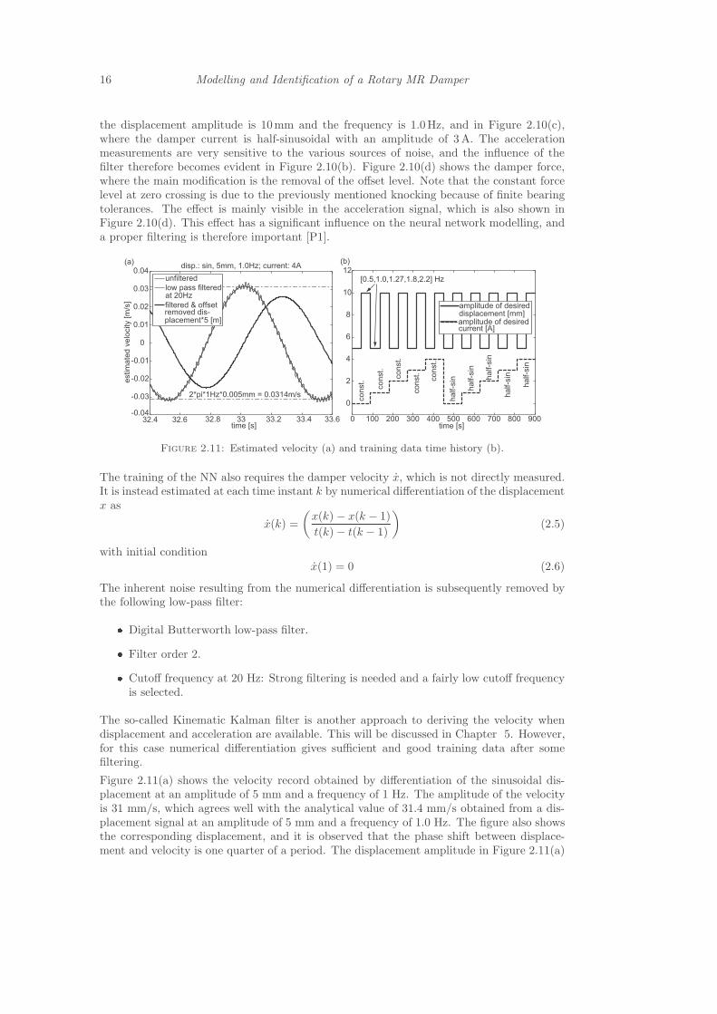
The training of the NN also requires the damper velocity x, which is not directly measured.It is instead estimated at each time instant k by numerical differentiation of the displacementx as
x(k) =
(x(k) − x(k − 1)
t(k)− t(k − 1)
)(2.5)
with initial conditionx(1) = 0 (2.6)
The inherent noise resulting from the numerical differentiation is subsequently removed bythe following low-pass filter:
� Digital Butterworth low-pass filter.
� Filter order 2.
� Cutoff frequency at 20 Hz: Strong filtering is needed and a fairly low cutoff frequencyis selected.
The so-called Kinematic Kalman filter is another approach to deriving the velocity whendisplacement and acceleration are available. This will be discussed in Chapter 5. However,for this case numerical differentiation gives sufficient and good training data after somefiltering.
Figure 2.11(a) shows the velocity record obtained by differentiation of the sinusoidal dis-placement at an amplitude of 5 mm and a frequency of 1 Hz. The amplitude of the velocityis 31 mm/s, which agrees well with the analytical value of 31.4 mm/s obtained from a dis-placement signal at an amplitude of 5 mm and a frequency of 1.0 Hz. The figure also showsthe corresponding displacement, and it is observed that the phase shift between displace-ment and velocity is one quarter of a period. The displacement amplitude in Figure 2.11(a)

2.3 Non-Parametric Neural Network Model of MR Damper 17
is multiplied by 2π. Figure 2.11(a) therefore demonstrates that the method in (2.5,2.6)leads to a velocity signal with the correct amplitude and phase compared to the measureddisplacement.
After the signal post processing, 10 steady state cycles of the data sets 1-19 in Table 2.1are isolated and then connected one after each other to get a single continuous time historyfor displacement, velocity, acceleration, current and force, respectively. The measured dis-placement data is selected as a sinusoidal signal at two different amplitudes of 5mm and10mm. These amplitude values are selected because the maximum amplitude of the damperdisplacement is expected to be located in the this range when operating on the shear framestructural model. Each amplitude is combined with five different frequencies in the rangefrom 0.5Hz to 2.2Hz, which contains the resonance frequency of the first vibration mode ofthe shear frame structure. In this way, 10 displacement data sets are produced. And sincevelocity is obtained by numerical differentiation also 10 velocity data sets are available. Thedamper current is produced in two ways. A constant current at different constant valuesfrom 0A to 4A are taken as the initial current input, while half-sinusoidal current recordsare also applied at five different amplitudes from 0A to 4A. Each amplitude is characterizedby five different frequencies from 0.5 Hz to 2.2 Hz. The amplitude range is selected between 0and 4A because these values are the limiting values of the MR damper. Figure 2.11(b) showsthe combination logic for the generation of the resulting time histories used for the neuralnetwork training and validation. It should be noted that the sets are always connected atzero crossings of the displacement. To have a reasonable amount of data for the trainingof the neural network, the time histories are finally downsampled from 1000 Hz to 200 Hz.The downsampling is very essential for proper training of neural network architecture.
2.3.2 Feedforward Backpropagation Neural Network Architecture
Two basic types of networks can be differentiated: networks with feedback and networkswithout feedback. For some networks it is characteristic that for every input vector laid onthe network, an output vector is calculated, which can be read from the output neurons.In this case there is no feedback. Hence, only a forward flow of information is present.Networks with this structure are called feedforward networks. Backpropagation is one ofthe effective tools in feedforward networks. Backpropagation is a systematic approach tothe training of multilayer neural networks, and it has a strong mathematical basis. It is amultilayer forward network using the extended gradient-descent based delta learning rule,commonly known as teh backpropagation of errors rule [74, 75]. A generalised multi-layerfeedforward backpropagation neural network with one layer of z hidden units is shown inFigures 2.12. The y output unit has woj bias and the z hidden unit has vok as bias. Thealgorithm used to train the neural network architecture is given in Table 2.3.
Backpropagation provides a computationally efficient method for changing the weights ina feedforward network, with differentiable activation function units, to learn a training setof input-output examples. The aim of this network is to train the net to achieve a balancebetween the ability to respond correctly to the input patterns used for training and theability to provide food responses to the input that are similar.
Modelling of a given system using the neural network tool requires basically three steps: (a)measurement of the input and output states of the system being considered, (b) choosingthe architecture of the particular neural network and (c) training the chosen architecturewith the measurement data [P1]. The neural architecture is characterised by:
� The kind of states used as inputs.
� The number of used previous values of input states.

18 Modelling and Identification of a Rotary MR Damper
1 1
bias
x1
x i
x n
bias
z
z
j
p
yk
ym
v ij
v 1j
v oj
w ok
v op
w jk
input outputhiddenlayer layer layer
Figure 2.12: Feedforward Backpropagation Neural Network
� The number of hidden layers and neurons per layer.
Because of the large variety of modelling parameters, the trial and error method is oftenapplied to find a neural network architecture with acceptable modelling errors. Using thetrial and error approach the training yields the best parameters for the chosen neural net-work architecture, but not necessarily the best neural network architecture with the bestparameters. The training algorithm of backpropagation involves four stages, viz.
� Initialization of weight
� Feed forward
� back propagation of errors
� updating of the weights and biases (if there are any)
At the first stage, which is initialization of weights, some small and random values areassigned. At the feedforward stage, each input receives an input signal and transmits thissignal to each of the hidden units. Each hidden unit then calculates the activation functionand sends its signal to each output unit. The output unit calculates the activation functionto form the response of the net for the given input pattern. During the backpropagation oferrors, each output unit compares its computed activation with its target value to determinethe error associated with this unit for the pattern concerned. Based on the error, the factoris computed and used to distribute the error at the output unit back to all units in theprevious layer. Similarly, the factor is computed for each hidden unit. At the final stage,the weight and biases are updated using the factor and the activation.
In the present work, a semi-systematic approach is used to find a neural network architectureclose to the optimum. The procedure is illustrated schematically in Figure 2.13. A numberof neural networks are trained to model the forward MR damper behaviour with the currentrecords and one, or several, of the time histories for displacement, velocity and acceleration,

2.3 Non-Parametric Neural Network Model of MR Damper 19
respectively, as input states. The number of previous states and the number of hiddenlayers and neurons are also varied. For all hidden layers the tangent sigmoid function ischosen as transfer function, while a linear transfer function is chosen for the output layer.All trained neural network approaches are based on the Levenberg-Marquardt optimisationmethod [74, 75], using the error(k) between the target force f(k) and the estimated force
f(k) by backpropagation. When the training is finished, the neural network architecture isstored and a new neural network architecture is trained for different input properties. Afterall possible combinations of input data have been used for training of the neural networksarchitecture, the particular neural network architecture with the smallest modelling error isstored as the best neural networks architecture. This neural networks architecture is thendenoted as the suboptimal neural network, because the transfer functions have not beenvaried. This systematic optimisation strategy shows the following trends:
x(k)
x(k)
i(k)
x(k)... n
o. d
ela
ys
selections
f(k)
f(k)+-
training
finished?
YES
store
all
data
Neu
ral N
etw
ork:
i) n
o. h
idd
en
la
ye
rs
ii) n
o. n
eu
ron
s/la
ye
r
transfe
rfunction:
- ta
nsig
fo
r a
ll la
ye
rs
- p
ure
lin fo
r o
utp
ut la
ye
r
change
selections
e(k)
Figure 2.13: Procedure to find suboptimal neural networks architecture
� Velocity is a mandatory input besides current. This is also confirmed by the largenumber of parametric MR damper models that are based on velocity and current asinput states.
� Using acceleration as additional input besides velocity and current increases the noisein the estimated force but not the model accuracy.
� Using displacement as additional input besides velocity and current does not decreasethe modelling error. This can be explained by the fact that the velocity is deter-mined from displacement (2.5). Another reason is that the rotary MR damper has noaccumulator which is known to introduce stiffness and displacement dependence.
� Using displacement and acceleration besides velocity and current as additional inputsdoes not decrease the modelling error.
� It seems that three previous values, two hidden layers and six neurons per hidden layerprovide a suitable compromise between modelling error and computational effort.
2.3.3 Neural Network Model Structure for MR Damper
For efficient operation of the backpropagation network, appropriate selection of the param-eters used for the training is necessary.
The initial weights will influence whether the net reaches a global (or only a local) minimumof error and if so how rapidly it converges. If the initial weight is too large the initial input

20 Modelling and Identification of a Rotary MR Damper
Delay
Delay
Delay
velocity(k)
velocity(k-1)
velocity(k-2)
velocity(k-3)
force(k)
Delay
Delay
Delay
current(k)
current(k-1)
current(k-2)
current(k-3)
input
input
O
lO
l(1) (2)
W (j)
Ol
(0)
O
l
(3)
Figure 2.14: neural network architectures of forward MR damper model
signals to each hidden or output unit will fall in the saturation region where the derivativeof the sigmoid has a very small value. If the initial weights are too small, the net input toa hidden or output unit will approach zero, which then causes extremely slow learning. Toget the best result the initial weights are set to random numbers between -0.5 and 0.5 orbetween -1 to 1.
Selection of learning rate is also very important to efficient neural modelling. A high learningrate leads to rapid learning, but the weights may oscillate, while a lower learning rate leadsto slower learning. In order to adopt an optimal learning rate, the learning rate is increasedto improve the performance and decrease the error value.
The motivation for applying the backpropagation net is to achieve a balance between mem-orization and generalization. It is not necessary to continue the training until the errorreaches a minimum value. The weight adjustment is based on training patterns. As longas the error for the validation decreases, the training continues. When the error begins toincrease, the net is starting to memorise the training patterns, and at this point the trainingis terminated [P1, P5].
The forward NN architecture that is found to minimize the error of the forward MR dampermodel is based on velocity and damper current as input states, with three previous valueseach, and it contains two hidden layers of six neurons each. The architecture of the forwardNN and the inverse NN are shown in Figure 2.14 and Figure 2.15, respectively. The transferfunction g(j) of the neurone of the two hidden layers are selected as a tangent sigmoidfunction, while the transfer function of the single output layer, i.e. layer 3, is selected asa linear function. If N (j) is the number of neurons in the jth layer then N (3) = 1, since
the output layer has only a single signal output. Let O(0)l be the R × 1 column vector
comprising the signal inputs to the 1st hidden layer. In this case R is 8 because of the twoinput variables: velocity and current, both with a current and three previous values. Let
O(j)l be the N (j) × 1 vector comprising the signal outputs of the jth layer. For the two
hidden layers the output are computed in terms of the sigmoid transfer function as
O(j)l = g(j)(W
(j)l O
(j−1)l + b
(j)l ) , j = 1, 2, 3 (2.7)
The matrix W(j)l contains the weights of the neural connections, while b
(j)l is the bias vector
of the jth layer, which is zero in the present application. The final output is O(3)l .

2.4 Model Validation 21
The architecture of the forward NN is shown in Figure 2.16 (a). Thus, the estimated forcebecomes
f(k) = NN
[x(k) x(k − 1) x(k − 2) x(k − 3)i(k) i(k − 1) i(k − 2) i(k − 3)
](2.8)
whereNN [..] represents the neural network function and i is the damper current. Figure 2.16(b) shows the corresponding neural network for the inverse damper model, which is alsobased only on velocity besides the damper force as input states. In order to estimate theMR damper current i(k) the neural network for the inverse model uses the actual and threeprevious values of the two input states,
i(k) = NN
[|x(k)| |x(k − 1)| |x(k − 2)| |x(k − 3)||f(k)| |f(k − 1)| |f(k − 2)| |f(k − 3)|
](2.9)
Irrespective of the sign of velocity and/or force, the damper current is always a positivequantity. Therefore, the neural network architecture is trained using the absolute values ofthe two input states. This approach helps to avoid the estimated current exhibiting negativespikes when, e.g. tracking a desired viscous damping force. Thus, the modelling error isminimized.
2.4 Model Validation
The model validation is carried out for independent and experimentally determined timerecords. Sections 2.4.1 and 2.4.2 consider the neural network of the forward and inversedamper model, respectively, while Section 2.4.3 demonstrates that the presented neuralmodel is able to emulate pure viscous damping.
2.4.1 Forward MR Damper Model
The forward MR damper model is validated using the validation data sets 1b-19b listed inTable 2.1. Due to the large amount of validation data, the measured and simulated forcedisplacement trajectories are compared for some selected tests. The selection is made suchthat the comparison is depicted for all displacement amplitudes, frequencies and currents.Figure 2.17 and 2.18 show the results for constant current, and Figure 2.19 and 2.20 thosefor half-sinusoidal current. As seen from the figures, the forward MR damper model is able
Delay
Delay
Delay
velocity(k)
velocity(k-1)
velocity(k-2)
velocity(k-3)
current(k)
Delay
Delay
Delay
force(k)
force(k-1)
force(k-2)
force(k-3)
input
input
O
lO
l(1) (2)
W (j)
Ol
(0)
O
l
(3)
Abs
Abs
Figure 2.15: neural network architectures of inverse MR damper model

22 Modelling and Identification of a Rotary MR Damper
estimated,
low pass
filtered velocity
x(k)
delay
delay
delay
.
x(k-1).
x(k-2).
x(k-3).
i(k)
delay
delay
delay
i(k-1)
i(k-2)
i(k-3)
post processed
current
post processed
force(k)
+_N
eu
ral N
etw
ork:
laye
r 1
, 6
ne
uro
ns, ta
nsig
laye
r 2
, 6
ne
uro
ns, ta
nsig
ou
tpu
t la
ye
r, 1
ne
uro
n, p
ure
lin
err
or(
k)
estimated,
low pass
filtered velocity
|x(k)|
delay
delay
delay
.
|x(k-1)|.
|x(k-2)|.
|x(k-3)|.
|f(k)|
delay
delay
delay
|f(k-1)|
|f(k-2)|
|f(k-3)|
post processed
force
post processed
current(k)
+_
err
or(
k)
abs
abs
(a) (b)
f(k)
f(k) i(k)
i(k)
Neu
ral N
etw
ork:
laye
r 1
, 6
ne
uro
ns, ta
nsig
laye
r 2
, 6
ne
uro
ns, ta
nsig
ou
tpu
t la
ye
r, 1
ne
uro
n, p
ure
lin
Figure 2.16: neural network architectures of forward (a) and inverse (b) MR dampermodels and their training.
to predict the main characteristics of the MR damper being considered with fairly goodaccuracy: The strong current dependent yield force is captured well, the slope of the pre-yield region is estimated very accurately in all cases [59, 60] and the force response due tothe aggregation and radial migration of particles [56], which is visible by the rather slowforce increase after the damper rod turns it direction, is also predicted satisfactorily. It isevident that all of the major damper characteristics are predicted significantly better for thehalf-sinusoidal current in Figures 2.19 and 2.19 than for the constant current case shownin Figures 2.17, 2.18. The harmonic signal for the current is most effective for the neuralnetwork training because the MR damper runs smoothly with harmonic current input atdifferent amplitudes and frequencies.
2.4.2 Inverse MR Damper Model
The inverse MR damper model is also validated using the validation data sets 1b-19b inTable 2.1. The results for constant current, two different displacement amplitudes andfour different displacement frequencies are shown in Figures 2.21(a) and (b). The estimatedcurrent shows significant spikes that might occur because the neural network architecturehas been trained not only with a constant current data but also with half-sinusoidal currentdata. This is partly verified by the fact that the spikes show the same frequency character-istics as the applied displacement. Similar results have also been reported in [68] and [72].This property might indicate that the neural network has difficulties estimating a constanttarget state accurately if the input states change periodically over time. In contrast to theprediction of the constant current, the prediction of the half-sinusoidal current is fairly ac-curate for different displacement amplitudes, frequencies and current amplitudes, as shownin Figure 2.21(c,d) and in Figures 2.22 and 2.23. Despite the apparent modelling error dueto the spikes of the estimated current, these spikes are rather small compared to e.g. thevalidation results presented in [68].
2.4.3 Emulation of Viscous Damping Using the Validated Model
In this section the forward and inverse models are used to determine how accurately pureviscous damping can be emulated by the rotary MR damper of the present study. Fig-ure 2.24(a) illustrates the flow chart of this simulation study. The velocity of the MR

2.4 Model Validation 23
displacement [mm]
forc
e [N
]
disp.: sin, 5mm, 1.0Hz; current: constant, 0A
measured forcepredicted force
(a)
−6 −4 −2 0 2 4 6-80
-60
-40
-20
0
20
40
60
80
displacement [mm]
forc
e [N
]
disp.: sin, 5mm, 0.5Hz; current: constant, 1A
measured forcepredicted force
(b)
−6 −4 −2 0 2 4 6−40
−30
−20
−10
0
10
20
30
40
−6 −4 −2 0 2 4 6−80
−60
−40
−20
0
20
40
60
80disp.: sin, 5mm, 1.27Hz; current: constant, 1A
displacement [mm]
forc
e [N
]
measured forcepredicted force
(c)
−10 −5 0 5 10
-150
-100
-50
0
50
100
150
displacement [mm]
forc
e [N
]
measured forcepredicted force
(d)
disp.: sin, 10mm, 0.5Hz; current: constant, 2A
Figure 2.17: Validation of forward MR damper model for constant current of 0A(a), 1A (b,c) and 2A (d) and different displacement amplitude and frequencies.
damper is assumed to be pure sinusoidal. This is a reasonable assumption for damping oflightly damped structures, where the structural response is typically dominated by reso-nance at the frequency of the critical vibration mode and with a slowly varying amplitudeenvelope. The desired control force is the product of velocity and the viscous coefficientc. The damper velocity and the desired control force are used as the input states for theinverse MR damper model, which then estimates the corresponding damper current thatis applied to the MR damper in order to generate a pure viscous force. This force is es-timated using the forward MR damper model. If the NN for the inverse and the forwardMR damper model are sufficiently accurate the simulated damper force should be compa-rable to the corresponding pure viscous damper force. The simulation results are shown inFigures 2.24(b-d). The simulated current in Figure 2.24(b) exhibits two significant spikeson top of the approximately half-sinusoidal time history. The first spike should not occurbecause the desired force decreases to zero. Hence, zero current would be the best choiceto track the desired viscous force as precisely as possible. The second current spike occurswhen the MR fluid is operated within the pre-yield region. This spike is therefore neededbecause the actual MR damper force at 0 A within the pre-yield region is smaller thanthe desired viscous force that increases rapidly at extreme displacement due to the ellipticforce displacement trajectory of viscous damping [48]. When the MR fluid is operated inthe post-yield region, the current shows approximately a half-sinusoidal behaviour becauseof the sinusoidal behaviour of the desired force, see Figure 2.22(c). The non-linear relationbetween yield force and current and the force response due to the migration and aggregationof the particles in the MR fluid [56, 60] are the reasons why the current does not show a purehalf-sinusoidal shape. Despite the mediocre estimate of the current at zero velocity and theslightly overestimated current in the pre-yield region, the time history of the damper force

24 Modelling and Identification of a Rotary MR Damper
−10 −5 0 5 10
−150
−100
−50
0
50
100
150
displacement [mm]
forc
e [N
]
disp.: sin, 10mm, 1.8Hz; current: constant, 2A
measured forcepredicted force
(a)
−6 −4 −2 0 2 4 6-250
-200
-150
-100
-50
0
50
100
150
200
250disp.: sin, 5mm, 1.0Hz; current: constant, 3A
displacement [mm]
forc
e [N
]
measured forcepredicted force
(b)
−6 −4 −2 0 2 4 6
−300
−200
−100
0
100
200
300
displacement [mm]
forc
e [N
]
disp.: sin, 5mm, 1.27Hz; current: constant, 4A
measured forcepredicted force
measured forcepredicted force
(c) (d)
−10 −5 0 5 10
-300
-200
-100
0
100
200
300
displacement [mm]
forc
e [N
]
disp.: sin, 10mm, 2.2Hz; current: constant, 4A
Figure 2.18: Validation of forward MR damper model for constant current of 2A(a), 3A (b) and 4A (c, d) and different displacement amplitude and frequencies.
in Figure 2.24 (c) and the force velocity trajectory in Figure 2.24 (d) demonstrate that pureviscous damping is in fact tracked fairly accurately at velocities larger than 0.05 m/s.
2.5 Summary
This chapter has initially demonstrated a modified bouc-wen modelling approach towardsrotary type MR damper and later described neural network based modelling of the forwardand inverse behaviour of a rotary MR damper using measured data for training and valida-tion. The measured data has been low-pass filtered in order to remove high-frequency signalparts that should not be considered by the neural network during training, and offset valueswere removed as well. The measured data resulting from two displacement amplitudes, fivefrequencies and both constant and half-sinusoidal current was combined sequentially to getone time history and downsampled from 1000 Hz to 200 Hz, so that the training data couldbe handled by the Matlab code for the given neural network architecture. It should be notedthat too much training data may create problems in neural network design. An optimisationprocedure has been presented for identifying a neural network architecture that minimisesthe error of the forward model. The procedure was tested with signals of measured displace-ment, measured velocity and measured acceleration or any combination of these three inputstates besides the measured current as input for the training. Furthermore, the numberof previous values of the input states and the number of hidden layers and neurons havebeen altered to obtain the best numerical fit. To limit the computational time of this nu-merical optimisation, the transfer functions for the hidden and output layers were fixed tothe tangent sigmoid function and the linear function, respectively. The present procedure

2.5 Summary 25
−6 −4 −2 0 2 4 6−80
−60
−40
−20
0
20
40
60
80disp.: sin, 5mm, 0.5Hz; current: half-sin, 1A, 0.5Hz
displacement [mm]
forc
e [N
]
measured forcepredicted force
−10 −5 0 5 10−80
−60
−40
−20
0
20
40
60
80
displacement [mm]
forc
e [N
]
disp.: sin, 10mm, 1.0Hz; current: half-sin, 1A, 1.0Hz
−10 −5 0 5 10−80
−60
−40
−20
0
20
40
60
80disp.: sin, 10mm, 1.27Hz; current: half-sin, 1A, 1.27Hz
displacement [mm]
forc
e [N
]
measured forcepredicted force
measured forcepredicted force
(a) (b)
(c)
−6 −4 −2 0 2 4 6−80
−60
−40
−20
0
20
40
60
80
displacement [mm]
forc
e [N
]
disp.: sin, 5mm, 1.8Hz; current: half-sin, 1A, 1.8Hz
measured forcepredicted force
(d)
Figure 2.19: Validation of forward MR damper model for half-sinusoidal current of1A and different displacement amplitude and frequencies.
demonstrated that the modelling error is not decreased significantly:
� if displacement and acceleration are taken as inputs in addition to velocity, and
� if substantially more than three past values of the inputs are taken into account, and
� if substantially more than two hidden layers with more than six neurons are considered.
The same neural network architecture, but with force instead of current, has also been usedto model the inverse MR damper behaviour. In this case, the absolute values of velocityand force are used for the training of the neural network that estimates current becausecurrent is always a positive quantity. This new approach helps to avoid the output currentbecoming negative when e.g. tracking a desired viscous force.
The trained forward and inverse MR damper models have been validated with measurementdata that is independent of the training data. The validation data comprised also tests attwo displacement amplitudes, five frequencies as well as both constant and half-sinusoidalcurrent. The validation shows that the forward model is able to predict the MR damperforce with high accuracy. Especially, the force response due to the migration and aggregationof the MR fluid particles is captured well, and the slope of the force displacement trajectoryin the pre-yield region is predicted accurately. The validation of the inverse MR dampermodel shows two particular characteristics. When the measurement data has been obtainedfrom constant current, the predicted current shows significant spikes at the same frequencyas the damper displacement, and only the mean value of the predicted current is reallyaccurate. In contrast, the prediction based on the half-sinusoidal current turns out to givevery accurate results for all amplitudes and frequencies used in the tests.

26 Modelling and Identification of a Rotary MR Damper
−6 −4 −2 0 2 4 6−150
−100
−50
0
50
100
150disp.: sin, 5mm, 1.27Hz; current: half-sin, 2A, 1.27Hz
displacement [mm]
forc
e [N
]
measured forcepredicted force
(a)
−10 −5 0 5 10−150
−100
−50
0
50
100
150disp.: sin, 10mm, 0.5Hz; current: half-sin, 2A, 0.5Hz
displacement [mm]
forc
e [N
]
measured forcepredicted force
−6 −4 −2 0 2 4 6-150
-100
-50
0
50
100
150disp.: sin, 5mm, 2.2Hz; current: half-sin, 2A, 2.2Hz
displacement [mm]
forc
e [N
]
measured forcepredicted force
(b)
−10 −5 0 5 10-150
-100
-50
0
50
100
150disp.: sin, 10mm, 1.8Hz; current: half-sin, 2A, 1.8Hz
displacement [mm]
forc
e [N
]
measured forcepredicted force
(d)(c)
Figure 2.20: Validation of forward MR damper model for half-sinusoidal current of2A and different displacement amplitude and frequencies.
The validated forward and inverse MR damper models are finally used to simulate theemulation of viscous damping. The simulation shows that the inverse model overestimatesthe current in the vicinity of zero velocity, i.e. in the pre-yield region, while the outputcurrent is quite accurate within the post-yield region. As a result, the force tracking erroris fairly large at small damper velocities but considerably small at velocities where the MRdamper is not operated in the pre-yield region.
This investigation shows that the neural network technique can be used to model the inverseMR damper behaviour and thus solve the force tracking task directly with a sufficiently smallforce tracking error.

2.5 Summary 27
a a+0.5 a+1 a+1.5 a+2
0
1
3
4
5
a a+0.5 a+1 a+1.5 a+2
0
1
3
4
5
cu
rre
nt [A
]predicted current for:
predicted current for:
predicted current for:
time [s]time [s]
(a) (b)
25 26 27 28 29
0
1
3
4
time [s]
0.5Hz, 5mm 1.0Hz, 5mm
44.5 45 45.5 46 46.5 47
1.27Hz, 5mm 1.8Hz, 5mm
time [s]
(c) (d)
4A; 5mm, 1.27Hz
2A; 5mm, 2.2Hz
0A; 5mm, 1.8Hz
predicted current for:
predicted current for:3A; 10mm, 0.5Hz
1A; 10mm, 1.0Hz
cu
rre
nt [A
]
0
1
3
4
cu
rre
nt [A
]cu
rre
nt [A
]
predicted
measuredcurrent
currentpredicted
measuredcurrent
current
Figure 2.21: Validation of inverse MR damper model for constant current (a, b) andhalf-sinusoidal current at 3A(c, d).
55 55.5 56 56.5 57 57.5
0
1
3
4
time [s]
(a)
2.2Hz,0.5Hz, 10mm5mm
84.5 85 85.5 86 86.5
0
1
3
4
time [s]
1.27Hz, 10mm1.0Hz, 10mm(b)
98.6 98.8 99 99.2 99.4 99.6
0
1
3
4
time [s]
2.2Hz, 10mm1.8Hz, 10mm(c) (d)
25.5 26 26.5 27 27.5 28 28.5 29
0
1
3
4
time [s]
1.0Hz, 5mm0.5Hz, 5mm
cu
rre
nt [A
]
predicted
measuredcurrent
current
cu
rre
nt [A
]cu
rre
nt [A
]
cu
rre
nt [A
]
predicted
measuredcurrent
currentpredicted
measuredcurrent
current
predicted
measuredcurrent
current
Figure 2.22: Validation of inverse MR damper model for half-sinusoidal current at3A (a-c) and 4A(d).

28 Modelling and Identification of a Rotary MR Damper
Table 2.3: Feed Forward Back Propagation Neural Network Algorithm
Parameters:x: Input training vectorx = (x1, ..., xi, ..., xn)t: Output target vectort = (t1, ..., ti, ..., tn)δk = error at output unit ykδj = error at output unit zjα = learning ratevoj = bias on hidden unit jzj = hidden unit jwok = bias on output unit kyk = output unit k
Step 1: Initialise weights.
Step 2: Input signal xi transmits to all units in the next hidden layers.
Step 3: For each hidden unit (zj, j = 1, ..., p), its weighted input signalzinj = voj +
∑ni=1 xivij
and activation functionZj = f(zinj)this signal transmits to all units in the output layer units.
Step 4: For each output unit (yk, k = 1, ...,m), its weighted input signalyink = wok +
∑pj=1 zjwjk
and activation functionYk = f(yink)
Step 5: For each output unit (yk, k = 1, ...,m) which receives a target patterncorresponding to an input pattern, the error information term is calcu-lated asδk = (tk − yk)f(yink)
Step 6: For each hidden unit (zj, j = 1, ..., n) which sums its delta inputs fromunits in the layer aboveδinj =
∑mk=1 δjwjk
The error information term is calculated asδj = δinjf(zinj)
Step 7: updating bias and weights (j = 0, ..., p) for each output unit(yk, k = 1, ...,m)weight correction term is ΔWjk = αδkzjand bias correction term is ΔWok = αδk.Therefore, Wjk(new) = Wjk(old) + ΔWjk
Wok(new) = Wok(old) + ΔWok
Updating bias and weights (i = 0, ..., n) for each hidden unit(zj , j = 1, ..., p),weight correction term ΔVij = αδjxi
bias correction term ΔVoj = αδjTherefore, Vij(new) = Vij(old) + ΔVij
Voj(new) = Vok(old) + ΔVoj .
Step 8: Test the stopping condition, either minimisation of error or number ofepoch is met or not.If not do step 2-7 again.Else if stop.

2.5 Summary 29
44.6 44.8 45 45.2 45.4 45.6 45.8 46 46.2 46.4
0
1
3
4
time [s]
1.8Hz, 5mm1.27Hz, 5mm
(a)
55 55.5 56 56.5 57 57.5
0
1
3
4
time [s]
0.5Hz, 10mm2.2Hz, 5mm
(b)
84.5 85 85.5 86 86.5
0
1
3
4
time [s]
1.27Hz, 10mm1.0Hz, 10mm
(c) (d)
98.4 98.6 98.8 99 99.2 99.4
0
1
3
4
time [s]
2.2Hz, 10mm1.8Hz, 10mm
predicted
measuredcurrent
current
predicted
measuredcurrent
current
predicted
measuredcurrent
current
predicted
measuredcurrent
current
curr
ent [A
]curr
ent [A
]
curr
ent [A
]curr
ent [A
]
Figure 2.23: Validation of inverse MR damper model for half-sinusoidal current at4A (a-d).
−0.15 −0.1 −0.05 0 0.05 0.1 0.15
-100
-50
0
50
100desired force
simulated force
velocity [m/s]
forc
e [N
]
0.2 0.4 0.6 0.8 1 1.2 1.4−1
−0.5
0
0.5
1
1.5
2
time [s]
disp.: sin, 20mm, 1.27Hz; emulation of viscous damping
velocity*5 [m/s]simulated current [A]
−300
−200
−100
0
100
200
300
desired force
simulated force
0.2 0.4 0.6 0.8 1 1.2 1.4time [s]
inverse model
velocity input (disp.: sin, 20mm, 1.27Hz)
c
desired force
simulated current
forward model
simulated force
viscous coefficient c
(a) (b)
(c) (d)
(data during 0.2-0.987s)
Figure 2.24: Simulated emulation of viscous damping: Flow chart (a), simulatedMR damper current (b) and simulated MR damper force (c-d).

Chapter 3
Modelling of a Flexible Structure
The present model identification technique uses a parametric approach to determining theparameters of the system model. Parameters may be represented as some kind of physicalquantities such as mass matrix, damping matrix and stiffness matrix. This chapter describesan experimental study to determine the system model parameters from test data. Theexperimental tests are performed using a shaking table. A five-mass shear frame structurehas been chosen for model identification and it is excited by ground acceleration by a shaker.It is assumed that all the mass of the floor is lumped at the centre of the mass of the floor.Hence, the sum of the mass of the individual plate and the mass of the four columns are takenas the lumped mass of the individual floor. The stiffness of the model is determined fromthe mode shape, which is constructed on the basis of the frequency transfer function fromthe test data. The damping matrix is determined from the estimated damping ratio froma free decay test. These five-degree-of-freedom structures possess five natural frequenciescorresponding to the number of degrees of freedom. When the structure is subjected to theexcitation, the resonance is induced if the frequency of excitation is close to each of one of thenatural frequencies of the structure. From the frequency response the resonance frequenciesare determined. Three data sets have been taken from the experimental setup. The firstset comprises data from the free decay test, where the five-mass system is initially excitedby sinusoidal base acceleration at the resonance frequencies. The excitation is then stoppedand the free decay response is used for determining the damping ratio of the vibration mode.The second set comprises data where the system is excited by sine sweep acceleration bythe shaker, and it is used for constructing the mode shape as well as for determining thestiffness matrix. The last data set is then used for validation of model parameters.
3.1 Overview of Experimental Setup
This chapter focuses on the parametric identification of the five-mass system subjected todynamic loading. A three-dimensional, five-floor building frame is used in the experiments.The structure is built in a shear frame configuration in which the building is rigidly at-tached to the shaking table platform. The parameter of the structure is explored throughsystem identification tests with free and forced vibrations. The ground acceleration is ap-plied by a shaker to the structure. The shaking table is driven horizontally by a hydraulicactuator. The measured ground acceleration is directly found from data acquisition hard-ware manufactured by OROS. The structure is kept vertically on the shaking table so thatthe base of the system is fixed to the shaking table. The accelerometers are fixed on eachfloor to measure the individual floor acceleration. The acceleration signal is taken fromthe accelerometer and amplified by an amplifier and sent to OROS for processing. Thedisplacements are also measured by laser sensors and used in the OROS data acquisitionhardware. All measurements are in volts and conversion into an appropriate unit is doneby multiplying measurement data by the corresponding conversion factor of the particulardevice. The experimental setup of the shaking table is shown in Figure 3.1, and a corre-sponding schematic diagram of the experimental setup is given in Figure 3.2. Furthermore,the properties of the plates and columns of the shear frame structure are given in Table 3.1.
30

3.1 Overview of Experimental Setup 31
Figure 3.1: Experimental Setup without MR Damper.
+ +
Hydraulic
Cylinder
Additional
Mass
Mass 1
Mass 5
Base
Piston
Shaking Table
Accelerometer
Mass 2
Laser Sensor
x5
x2
x1
xg..
a5
a2
a1
m2
m5
m1
Figure 3.2: Schematic diagram of Experimental Setup

32 Modelling of a Flexible Structure
Table 3.1: Structural parameters.
Plate Length 315 mm E(steel) 21× 1010N/m2
(Steel) Width 215 mm ρ(steel) 7.9× 10³Kg/m3
Thickness 20 mm σ(steel) 0.3
Column Length 370 mm Distance between two column
(Steel) Width 10 mm Longitudinal 300 mm
Thickness 4 mm Lateral 175 mm
3.1.1 Measurement Sensors
Accelerometers are used to measure the acceleration of the shaking table as well as formeasuring the response of each individual acceleration of the five-floor structure. The ac-celerometers are of the PCB 3701G3FA3G type and produce an output of 3 volts with arange of 3g. The supply voltage of the accelerometer is 27 V. Laser sensors optoNCDT 2200are used to measure directly the displacement of the plates. Three laser sensors are availablein the lab. They are mounted on a stand which is fixed on the ground. Two sensors are fixedin first and second plate positions. The third is positioned to measure the displacement ofthe third, fourth or fifth plate, depending on the goal of the test. The laser distance sensoremploys triangulation measurement principles so that it projects a beam of visible laser lightthat creates a spot on a target surface. Reflected light from the surface is viewed from anangle by a digital CMOS line scan camera inside the laser sensor. The displacement of thetarget is computed from the image pixel data. The supply voltage of the laser sensor is 24 V.This laser can measure an output of 20 mm. The conversion factors for the laser sensors arefound by calibration tests and are given in Table 3.2. A photo of one of the accelerometersand the laser sensor is shown in Figure 3.3.
3.1.2 Hydraulic Actuators and Control Unit
The hydraulic control unit is shown in Figure 3.4. The hardware setup is manufactured byInstron. The hydraulic cylinder used in the shaking table is a Schenk hydraulic model. Themaximum displacement of hydraulic cylinder is 180 mm. The static force is 40 kN and thedynamic force is 80 times that of the static force.
Table 3.2: Conversion factors for sensor data.
Sensors Acceleration Displacement Force Ground
(PCB3701G3FA3G)
(opto NCDT2200) displacementfrom OROS
conversionfactor
g(≈ 9.81) m/s2/V 0.0109 m/V 50 N/V 0.018 m/V

3.1 Overview of Experimental Setup 33
Figure 3.3: Laser Sensor and Accelerometer
Figure 3.4: Hydraulic Control Unit
3.1.3 Filtering
The sensor data from the laser sensor and the accelerometer always has some noise. Thus,before applying the sensor data to modelling, filtering of the signal is necessary. The low-pass reduces the amplitude of the signal parts above the cut-off frequency, while a high-passfilter conversely reduces the signal part below the cut-off frequency. Thus, the low-pass filteris effectively applied to reduce signal and measuring noise, while the high-pass filter can beused to remove any off-set in the data. The two filter types can be combined in a band-pass filter, where frequencies (well) within the band are passed through the filter. For thefree vibration decay test the band pass filter is applied and the frequency band is selectedat approximately the resonance frequency of the corresponding mode because in the freevibration decay test, only the excited mode is considered. However, for the sine sweep test

34 Modelling of a Flexible Structure
the band is selected in between a frequency lower than the first resonance frequency and afrequency higher than the fifth resonance frequency, so that the DC part of the signals andthe noise are located at higher frequencies.
For the free decay test for first mode peak detection, the structure is excited using sinusoidalground displacement with a frequency equal to the first mode resonance frequency. Thesignal is filtered through a band pass filter where the cutoff frequencies are chosen aroundthe first resonance frequency.
For effective filter design the following points are considered.
� Type of filter: Digital Butterworth band pass filter.
� Selection of filter order.
� Selection of suitable high-pass and low-pass cutoff frequency for band pass filter.
The applied band pass filter properties for acceleration and displacement measurements forthe sine sweep test and the free decay test are discussed in the following sections.
3.2 Model Parameter Identification
The method for parameter identification is presented in the following subsections. Thestructural model has three main parameters: Mass matrix, stiffness matrix and dampingmatrix. The structural model is considered as a shear frame structure. The mass matrix isformulated on the basis of measuring the lumped mass of each floor, the damping matrix isderived from a free vibration test and the stiffness matrix is calculated from a modal analysis.The damping matrix in a modal coordinate system is constructed by a diagonal matrix wherethe diagonal elements are the damping coefficients for each mode. The damping coefficientis finally derived from the damping ratios of the individual vibration modes.
The damping ratio is evaluated mainly by the following three methods. First of all, thepeaks of the measurement signal are identified and used for constructing the decay profile.The first method is based on linear fitting and the second on a logarithmic fitting algorithmand the third on the average value of the damping ratio of two consecutive peaks. Peaks ofthe signals are calculated for the entire range of the measurement signal. However, the onlyrange considered is that where the measurement signal decays. The first and the secondmethods fit the peak values of the signal with linear and logarithmic curves in the regionwhere the measurement signal decays.
The damping ratio may be estimated from the ratio of adjacent local maxima during a freevibration response u(t) at time t and after a period at time t+ Td. For logarithmic fitting,the damping ratio is written as
ζ =δ√
(4π2 + δ2)(3.1)
where δ is the logarithmic decrement which is as follows
δ = ln
(x(t)
x(t+ Td)
)(3.2)
The damping ratio is evaluated from the free decay test and thus the damping matrix isformulated. The sine sweep test is conducted next to evaluate the resonance frequenciesof all the modes to identify the mode shape from the frequency transfer function of themeasurement signal.

3.2 Model Parameter Identification 35
Table 3.3: Resonance Frequencies.
Mode Number 1 2 3 4 5
Resonance Frequency (Hz) 1.23 3.83 6.13 8.05 9.34
Resonance Frequency (rad/s) 8.0 24.2 38.4 49.9 58.3
3.2.1 Sine Sweep Test
For evaluating the dynamic properties of a structure, a forced vibration test is performedusing sinusoidal (harmonic) loading over a range of frequencies that include all modal res-onance frequencies. The idea is to excite the structure with harmonic loading over a rangeof frequencies so that at some frequency the structure experiences resonance. Resonanceoccurs when the frequency of the excitation is equal to the natural frequency of the struc-ture. At the resonance frequency, the structure experiences its largest response, comparedto any other excitation frequency. The measured acceleration data from the sine sweep testusing Fast Fourier Transform (FFT) analysis and the five resonance frequencies correspond-ing to the main five degrees of freedom have been identified approximately. The resonancefrequencies for the corresponding five modes are identified from Figure 3.5, which shows thefirst floor acceleration data in the frequency domain. The resonance frequencies are givenin Table 3.3.
For the sine sweep test the band is determined by frequencies lower than the first resonancefrequency and higher than the fifth resonance frequency. Hereby, the DC part of the signalsand the noise are located at even higher frequencies. For the sinus-sweep test the high-passand low-pass cutoff frequencies are considered as 0.2 Hz and 14 Hz, respectively, whichincludes all the modes. The order of the band pass filter is kept low so that the mainproperties of the measurement signal are unaltered. For the sine sweep test data, the order
0 5 10 15 20 25 30 35 40
10−8
10−6
10−4
10−2
100
PS
D(a
1) [m
2 /s3 ]
unfilteredlow pass filteredhigh pass filteredband pass filtered
frequency [Hz]
Figure 3.5: Filtered and unfiltered acceleration in the frequency domain

36 Modelling of a Flexible Structure
1 1.05 1.1 1.15 1.2 1.25 1.3 1.35 1.4 1.45 1.50
10
20
30
40
Frequency (Hz)
Mag
nit
ud
e
a1a2a3a4a5
1 1.05 1.1 1.15 1.2 1.25 1.3 1.35 1.4 1.45 1.5−2
−1
0
1
2
Frequency (Hz)
Ph
ase
Figure 3.6: Magnitude and phase angle from transfer function
is chosen as 3. The five resonance frequencies for the corresponding five modes are alsofound from first five modal resonance frequency from Figure 3.5. It also shows some otherhigher frequencies which are mainly arrives due to flexible support. The sine sweep testis conducted to evaluate the mode shape for five different modes and construct a modalmatrix and to evaluate the stiffness matrix from the modal matrix. The procedure forstiffness matrix identification is discussed below:
� Estimation of the mass: The mass, mi, of each floor of the structure is determined.The plate and four columns are lumped together to determine the corresponding massof the floor. The mass matrix is expressed as
M =
⎡⎢⎢⎢⎢⎣
m1
m2
m3
m4
m5
⎤⎥⎥⎥⎥⎦ (3.3)
� Identification of the resonance frequency: The resonance frequency is evaluated fromthe location of the peak in the frequency response diagram. The resonance frequenciesfor the corresponding five modes are found from the frequency response diagram shownin Figure 3.5.
� Construction of the frequency transfer function: The transfer functions in the fre-quency domain between the output signals (measured floor acceleration) and the in-put (ground acceleration) are determined. The relationship between the input groundacceleration (ag) and output floor acceleration (ai) is modelled by the linear, time-invariant transfer function Tgi. The transfer function is the quotient of the cross powerspectral density, Pgi(ω) of ag and ai, and the power spectral density, Pgg(ω) of ag withitself. The frequency transfer function is then expressed as
Tgi(ω) =Pgi(ω)
Pgg(ω)(3.4)

3.2 Model Parameter Identification 37
−50 0 50
0
2
4
6
−20 0 20
0
2
4
6
−10 0 10
0
2
4
6
−5 0 5
0
2
4
6
−5 0 5
0
2
4
6
Figure 3.7: Mode Shape
� Evaluation of the magnitude and phase from the frequency response of the transferfunction: The magnitude and phase are determined from the frequency transfer func-tion for each of the five modes. The magnitude and phase for all floors for the firstmode are shown in Figure 3.6. In this diagram, the magnitude and phase are deter-mined from the transfer function constructed between the first floor acceleration andthe ground acceleration. Similarly, all other transfer functions have been derived.
� Determination of the maximum magnitude and corresponding phase for all five modes:The magnitude and phase of each of the five floors for all five modes are evaluated.The peak magnitude and the corresponding phase angle for the first mode are shownin Figure 3.6. The frequency at which maximum magnitude is determined is actuallyrepresented as the resonance frequency of the corresponding mode. From this diagramthe actual resonance frequency for the corresponding mode is also evaluated.
� Construction of the mode shapes for all five modes using the magnitude and phasevalues: The maximum magnitudes of the five floors for the corresponding modes areconsidered for construction of the mode shape. The phase at the corresponding fre-quency where the maximum peak occurs is used to determine the sign of the magnitudefor mode shape. Figure 3.7 shows the mode shape diagram for all the five modes.
� Construction of the non-dimensional mode shape: The magnitude of each floor isnormalized by dividing the maximum amplitude by the corresponding mode and bydividing the maximum magnitude of the floor at the corresponding floor, so that thedimensionless mode shape is formed and the magnitudes are in between 0 to 1. Thenon-dimensional mode shape is shown in Figure 3.8. This non-dimensional mode shapeis compared with the theoretical mode shape of a shear frame which has one free end.The theoretical mode shape is assumes to be sinusoidal. The comparison is also shown

38 Modelling of a Flexible Structure
−2 0 2
0
2
4
6
−2 0 2
0
2
4
6
−2 0 2
0
2
4
6
−2 0 2
0
2
4
6
−2 0 2
0
2
4
6
Measurement
Sinusoidal
Middle position
Figure 3.8: Mode Shape - Non-dimensional
in Figure 3.8 and the non-dimensional mode shape shows good agreement with thetheoretical mode shape.
� Formation of modal matrix: From the mode shape, the modal matrix is formed inmodal coordinates
U =
⎡⎢⎢⎢⎢⎣
0.349 0.861 1.000 0.868 0.4530.604 1.000 0.117 −0.979 −0.8380.773 0.449 0.941 0.119 1.0000.920 −0.356 −0.464 1.000 −0.8271.000 −0.952 0.789 −0.596 0.319
⎤⎥⎥⎥⎥⎦ (3.5)
where each column represents the normalised magnitude of each of five nodes at thecorresponding mode. The column number represents the mode number.
� Formulation of the stiffness matrix in modal coordinates: The stiffness matrix in modalcoordinates Km is a diagonal matrix where the the diagonal elements of the matrix areconstructed from the mass element and the corresponding modal resonance frequency.The modal stiffness is determined from the following expression
ki = ω2i mi (3.6)
where mi is the modal mass associated with the mode shape matrix U and ωi are theresonance frequencies determined from the peaks in the acceleration spectrum. Thestiffness matrix in modal coordinate is calculated as
Km =
⎡⎢⎢⎢⎢⎣
k1k2
k3k4
k5
⎤⎥⎥⎥⎥⎦ (3.7)

3.2 Model Parameter Identification 39
� The diagonal element of the modal matrix Km is taken and the stiffness matrix inCartesian coordinates, K is found by
K = (UT)−1KmU−1 (3.8)
3.2.2 Free Vibration Test
In this section, free vibrations are obtained by initially imposing a harmonic force by ashaker, and when the structure is vibrating at the desired frequency the shaker excitationis then stopped and free vibrations at the desired frequency occur. This free vibration canbe analysed based on the concept of the logarithmic decrement. However, for higher modesthe free vibration response is not a suitable method due to the inherent ambient noise.
For the free vibration decay test the Butterworth band pass filter is applied and the frequencyband is selected around the resonance frequency of the corresponding mode because in thefree vibration decay test only the excited mode is considered.
For the free decay test for first mode peak detection, the structure is excited using sinusoidalground displacement with a frequency equal to the first mode resonance frequency. Thesignal is filtered through a band pass filter where the cutoff frequencies are chosen aroundthe first resonance frequency. The following properties of the band pass filter are considered.
� A band pass Butterworth filter is used.
� The high-pass cut-off frequency is selected as ωi − ωcut where ωi is the resonancefrequency for the corresponding mode and the margin to the filter limit is ωcut =π rad/s.
� The low-pass part of the filter the cut-off frequency is selected at ωi + ωcut.
� The order of the filter is in this case chosen as 5.
The effect of applying the band pass filter to noise reduction is demonstrated in time andin the frequency domain for the 1st floor for free vibration data and is shown in Figure 3.9.The procedure for the damping ratio identification based on free vibration test data is asfollows:
� Measurement of peak value in decay zone: The peak of each cycle is identified fromthe free vibration response when the signal is in decay. Figure 3.10 (a) shows all thepeaks detected in the decay envelope.
� Estimation of curve fitting: From the peaks of the data in the decay zone, a curve fittingis estimated using exponential or linear fitting. The curve fitting using exponentialand linear fit are shown in Figure 3.10. The exponential fit is working better whencompared to linear fit on an average level, while the linear fit is fairly good at theinitial part of the free decay.
� Finding the damping ratio : The damping ratio, ζi is evaluated from the decay rateof the curve. This done by evaluating the decay rate of the logarithmic and the linearcurve fitting. The logarithmic decay is calculated from (3.1). An alternative methodfor determining the damping ratio is finding the damping ratio between two consecutivepeaks, and the computing the final values as the mean value from the individual peak-to-peak values in the decay. Figure 3.10(b) shows the relationship between amplitudeand damping ratio from the logarithmic fitting and the point to point estimation. It isfound that the average of the point to point damping ratio is almost the same as the

40 Modelling of a Flexible Structure
Figure 3.9: Filtered and unfiltered acceleration in the time domain
logarithmic estimate. From the decay tests the damping ratios have been estimatedfor the five vibration forms as
ζ1 = 0.0030 , ζ2 = 0.0024 , ζ3 = 0.0020 , ζ4 = 0.0015 , ζ5 = 0.0010
When the structure is in free vibrations the applied loading is zero. In this case theequation of motion is
Mx+Cx+Kx = 0 (3.9)
In modal coordinates the damping matrix C is transformed into a diagonal matrixCm, when assuming orthogonal damping. The elements in the diagonal are then the
0 20 40 60 80−1
−0.5
0
0.5
1AccelerationPeak ValueExponential fit
Acceleration,m/s2
Time, s0 0.2 0.4 0.6 0.8
0.008
0.01
0.012
0.014
0.016
0.018
0.02
amp
exponential fitpoint to point
Dampingration,ζ
Figure 3.10: Peak detection and exponential fitting (a) and damping ratio (b)

3.3 Equations of Motion 41
viscous damping parameters ci in modal coordinates.
C = (UT)−1CmU−1 (3.10)
The diagonal element of the damping matrix in modal coordinate can then be writtenin terms of the estimated damping ratio ζi as
ci = 2ζi√miki (3.11)
where mi and ki are the modal mass and stiffness components for the correspondingmodes, which have already been determined via the sine sweep test.
3.3 Equations of Motion
The equation of motion for a shear frame structure with external excitation can be writtenas
Mx+Cx+Kx = fe (3.12)
The degrees of freedom of the model are contained in the vector x, while M, C and K arethe associated mass, damping and stiffness matrix, respectively. The vector fe representsthe external loading.
3.3.1 Mass Matrix
For individual plate mass calculation the mass of the plate and the four columns have beentaken as a lumped mass and the representative mass of the individual floor is then found as5.95 kg. The mass matrix in Cartesian coordinates is then determined as
M(i, i) = mmass + 4mcolumn , M(i, j) = 0 , if i �= j (3.13)
Thus, the matrix matrix is assumed diagonal with identical diagonal elements.
3.3.2 Stiffness Matrix
First, the mode shape vector ui and the radial eigenfrequency ωi of mode i are estimatedfrom the measured transfer functions. The measured mode shapes are normalised to unityat a height of 5.5 floors, where it corresponds to the mode shapes of a sinusoidal function.The comparison is shown in Fig. 3.8. The measured mode shape matrix U yields the massmatrix in modal coordinates
Mm = UTMU (3.14)
which is found to have predominant diagonal elements. Therefore, the stiffness matrix inmodal coordinates Km is approximated as follows
Km(i, i) = ωi2Mm(i, i) , Km(i, j) = 0 , if i �= j (3.15)
The back transformation leads to the desired stiffness matrix in Cartesian coordinates,
K = (UT )−1
Km(U)−1
(3.16)
which is fully occupied. However, the elements outside the tri-diagonal band are smallcompared to the main tri-band, which verifies that the present structure can be modelledas a shear frame structure.

42 Modelling of a Flexible Structure
3.3.3 Damping Matrix
The damping matrix is determined from free vibration test. The diagonal element of thedamping matrix is determined from the corresponding diagonal element of mass and stiffnessmatrix. The damping ratio ζi is found for each corresponding mode. The diagonal elementin the damping matrix Cm in modal coordinates is found from
Cm(i, i) = 2ζi√Km(i, i)Mm(i, i) (3.17)
The other elements of the damping matrix are considered as zero. The damping matrixin modal coordinates Cm is estimated as a diagonal matrix where the diagonal elementsare determined from (3.17). The damping matrix in Cartesian coordinates C is determinedfrom back transformation and expressed as
C = (UT )−1
Cm(U)−1
(3.18)
This matrix is also fully occupied, and is not dominant as much by the tri-diagonal band.This demonstrates the difficulties in the estimation of structural damping.
3.3.4 Model Verification
The equation of motion in (3.12) is formulated in the state space representation and solved inMatlab/Simulink using the measured ground acceleration as excitation and without externaldamper. The model validation is depicted in Figure 3.11 for two selected accelerations in thetime domain and in Figure 3.12 for two other selected accelerations in the frequency domain.The results show a small modelling error in both the time and the frequency domains. Thenatural frequencies and damping ratios are determined by solving the state-space eigenvalueproblem associated with the equation of motion in (3.9). The frequencies are determinedas:
ω1 = 8.0 , ω2 = 24.2 , ω3 = 38.4 , ω4 = 49.9 , ω5 = 58.3
which agree very well with the experimental frequencies given in Table 3.3. The modaldamping ratios are determined as
ζ1 = 0.0035 , ζ2 = 0.0024 , ζ3 = 0.0074 , ζ4 = 0.0059 , ζ5 = 0.0012
and they match well with the experimental values provided previously. Thus, the mainreason for some deviations in the comparison of experimental and numerical response recordsis most likely the error in measuring decay in free vibration test.
3.4 Summary
This chapter considers the system modelling of a flexible structure using an experimentalprocedure and presents validation results from the numerical model. A five-mass shearframe structure has been chosen for the model identification. The stiffness of the model isdetermined from the mode shapes, which are constructed from a frequency transfer functionbased on vibration test data. The damping matrix is determined from the estimated dampingratios from a free decay tests. From the frequency response the resonance frequencies aredetermined, and the validation of the model shows good agreement with the measurementdata.

3.4 Summary 43
Figure 3.11: Validation of shear frame model in time domain.
0 5 10 15
10-8
frequency [Hz]
PS
D(x
2)
[m2/s
3]
measured
0 5 10 15frequency [Hz]
0 5 10 15frequency [Hz]
0 5 10 15frequency [Hz]
10-6
102
100
..
simulated
10-8
PS
D(x
5)
[m2/s
3]
10-6
102
100
..
10-8
PS
D(x
2)
[m2/s
3]
10-6
102
100
..
10-8
PS
D(x
5)
[m2/s
3]
10-6
102
100
..
(a) (c)
(b) (d)
measured
simulated
Figure 3.12: Validation of shear frame model in frequency domain.

Chapter 4
Control Strategies and Simulation
In civil engineering, the mitigation of structural vibration induced by dynamic loads, such asearthquake or wind loads using appropriate control strategy is one the most challenging taskfor structural engineers. Several control strategies based on passive, active or semi-activecontrol methods are investigated for finding effective solution to mitigate the structural vi-bration. In recent year semi active control device like MR damper got considerable attentiondue to its reliability, adaptability, cost effectiveness and fail safe mechanism.
Passive damping devices are purely dissipative and are not controlled during motion of thedamper. They do not have external power requirement and are very stable since they donot add energy but only dissipate it, thus yielding a very robust device [2]. Active damperscan unlike passive dampers be adapted to the dynamic loading. An active damper systemconsists of of actuators and sensors coupled by active controller, which gives a feedbackloop which can be position, velocity, acceleration or force. The active dampers are drivenby an external power supply which is a major drawback of using active damper during anearthquake. Active dampers are very stable and robust [5].
Semi-active dampers like MR damper have similarity with active dampers, but they havelower power requirements and also stable as passive control device. In fact, maximum MRdampers can operate on battery power, which is a big advantage during an earthquake. Sosemi-active control can combine the advantages of active and passive control [9]. The staycable damping potential due to controlled MR dampers has been investigated by simulation,laboratory and field tests in many research projects [42, 43, 46, 76]. Weber et al. [36, 47, 77]demonstrated different passive and semi-active control strategies on cable bridges. Moreover,the vibration reduction of civil engineering structures such as buildings, bridges and modelsof these structures with controlled MR dampers has been simulated and tested [79] - [83]and in tuned masses [37] in order to make these passive devices adaptive. Many differentclipped active, semi-active and passive control laws for MR dampers have been tested.Clipped optimal control schemes as presented in e.g. [14, 76], clipped viscous damping withnegative stiffness as described in e.g. [36], semi-active algorithms [30, 48] and passive controllaws such as emulated viscous damping [46], controlled friction damping [30, 32, 42, 84],controlled energy dissipation [47] and passive control [77]. In semi-active control the trackingof a desired force is a main issue and the problem has been solved in various ways. TheHeaviside step function approach that requires measuring the actual MR damper force ispresented by Dyke et al. [14]. The Bingham model was used to derive the current forgiven measured damper velocity and desired force [36, 46]. Dahl model is also presented byAguirre et al. [85] which can also be used as MR damper model. The LuGre friction approachwas used to model the MR damper behaviour and the validated model was then used asobserver [56, 54, 55]. A mapping approach based on tests of the MR damper connectedto the cable is presented in [47], neural network based force tracking approaches have beendeveloped and also fuzzy logic and other methods have been adopted to capture the inverseMR damper dynamics [86] - [95].
In recent years, the structural damping due to the emulation of a negative stiffness forcebesides the damping force in the MR damper was investigated in several research projects [31,
44

4.1 Damping of Flexible Structures 45
32, 34]. It is shown in [36] that larger structural damping is achieved because the negativestiffness force increases the motion in the damper, which makes it possible to dissipatetwo times more energy per cycle in the damper than the optimal viscous damper [96]. Itwas shown in [97] that clipped optimal control of a cable with semi-active damper resultsin approximately the same control force as clipped viscous damping with negative stiffness.Consequently, the approach of clipped viscous damping with negative stiffness for semi-activecable damping is a powerful control approach since its realisation requires only measuringthe damper displacement, it generates twice as much structural damping as optimal viscousdamping and avoids the complex state estimation which is essential for optimal controlapproach.
This chapter therefore investigates the semi-active damping of a five-degree-of-freedom (5DOF) shear frame structure with an MR damper. The tested control laws are optimalviscous damping as benchmark, viscous damping with negative stiffness [P4], optimal semi-active damping, i.e. friction damping with negative stiffness [P2] and neural network basedreference control strategy [P5]. All four control laws are designed based on a validated shearframe model described in Chapter 3. The force tracking task is solved with a neural networkmodel [P1] that describes the inverse dynamics of the MR damper. Details are discussedin Chapter 2. It is described how the neural network is implemented in simulation usingMatlab/Simulink. The structural damping resulting from the above-mentioned control lawsis calculated and compared each other for the first excited mode. The comparison showsthe effectiveness of negative stiffness. In the closed loop simulation the control approacheshas acceptably small force tracking error. This tracking error is mainly due to the MRdamper current, which is generated by the neural network, is fairly noisy. It is shown thatthe neural network approach can be used to track the desired force. A thorough descriptionof the novel neural network approach is given in Chapter 2. The descriptions of the variouscontrol strategies and simulation results are discussed in the following sections.
4.1 Damping of Flexible Structures
In dynamic analysis of flexible structures the structural model is typically modelled by finiteelements or determined by experimental modal analysis and free vibration test, so that theequation of motion can be written in the form
Mx+Cx+Kx = −wf + fe (4.1)
where the vector x contains the generalised displacements and a dot denotes time differenti-ation, and K, C and M are the structural stiffness, damping and mass matrix, respectively.The external load is represented by the vector process fe. Finally, a single damper is actingon the structure, where f represents the damper force and w is the connectivity vector de-scribing the location of the damper and represented as w = [1, 0, ...]T for the present shearframe problem. The base excitation is represented as fe = MI(−xg) where xg is the groundacceleration and I = [1, 1, ...]T is unity vector. The schematic illustration of the shear framestructure with rotational MR damper is shown in Figure 4.1.
For linear damper models the characteristics of the damper are conveniently formulated inthe frequency domain as
f(ω) = H(ω)x (4.2)
where H(ω) is a frequency dependent damper function. In the frequency domain x is simplythe response amplitude of the damper motion. In the next section a system reduction proce-dure for flexible structures with local dampers is presented. This procedure leads to explicitexpressions for the complex-valued natural frequency, which can be used to determine theoptimal damper tuning leading to maximum modal damping [P2, P4].

46 Control Strategies and Simulation
+ +
Mass 1
Mass 5x5
x1
xg..
MR Damper
Base
Figure 4.1: Schematic diagram of shear frame structure with MR damper.
4.2 Two-Component System Reduction and Modal Damping
The effective damping of the structure is evaluated in terms of its modal damping, where thepresence of the external damper generates non-proportional damping with complex-valuednatural frequencies and mode shapes. System reduction techniques based on undampedmode shapes require a large number of terms to give satisfactory results. The analysis ofthe damper modal vibrations is described by the two-component system reduction techniqueintroduced by Main and Krenk [29]. Høgsberg and Krenk [96] have implemented this tech-nique for finding the optimal viscous parameter for cable damping. In this formulation theresponse of the structure is represented by a linear combination of the two limiting modeshapes for the structure without damper u0 and for the structure with the damper fullylocked u∞, respectively. The linear combination can then be written as
x = u0r0 + u∞r∞ = Sr (4.3)
The first term represents the classical undamped case, while the second term introducesthe local effect of the damper described in terms of its ability to lock the structure in itslocation. The detailed process is also discussed in [P2, P4]. The relative weighting betweenthe two limiting cases is governed by the coordinates of the reduced subspace: r = [r0, r∞]T .Similarly, the limiting mode shapes are assembled in the modal matrix: S = [u0,u∞]. Theundamped mode shape is governed by the classical generalised eigenvalue problem:
(K− ω20M)u0 = 0 (4.4)
A smaller eigenvalue problem exists for the case where the damper link is fully locked,defining ω∞ and u∞. The locked mode shape u∞ is by construction orthogonal to theconnectivity vector which yields the identity wTu∞ = 0. Both limiting mode shapes arereal-valued and conveniently normalised to unit modal mass,
uT0 Mu0 = 1 , uT
∞Mu∞ = 1 (4.5)
Consequently, the limiting natural frequencies are given in terms of the modal stiffness,
uT0 Ku0 = ω2
0 , uT∞Ku∞ = ω2
∞ (4.6)

4.3 Control Strategies 47
The limiting mode shapes and natural frequencies are all real-valued and may be deriveddirectly from the associated generalised eigenvalue problems.
The equations of motion can be described in the reduced two-dimensional subspace bysubstitution of (4.3) into (4.1) followed by pre-multiplication by the limiting mode-shapes.In the frequency domain the reduced system of equations can be written in the followinghomogeneous form when free vibrations are considered
[ω20 − ω2 + u2
0H κ(ω20 − ω2)
κ(ω20 − ω2) (ω2
∞ − ω2)
] [r0r∞
]=
[00
](4.7)
The amplitude of the mode shape in the damper location is u0 = wTu0 and κ = uT∞Mu0
represents the coupling between the two limiting mode shapes. Free vibrations require asingular matrix which yields a characteristic equation in ω in e.g. Main and Krenk [29]. Thischaracteristic equation can be rewritten in an explicit, given solution by assuming that thecoupling parameter κ � 1. This solution is conveniently expressed in the following compactform
ω − ω0
ω∞ − ω0�
μH
1 + μH(4.8)
In this expression the modal flexibility parameter is given as
μ =u20
ω2∞ − ω2
0
�u20
2ω0(ω∞ − ω0)(4.9)
The modal damping ratio is determined as the relative imaginary part of the complex valuednatural frequency, which can be approximated by ζ =� Im[ω − ω0]/|ω|. In the case ofresponse dominated by resonance the magnitude of the structural is approximately inverseproportional to the damping ratio of the dominant mode. Thus, a suitable optimal tuning isbased on the maximization of the modal damping ratio with respect to the gain parameterof the particular control strategy. If the approximation |ω| � ω0 is introduced the dampingratio can be written as
ζ =ω∞ − ω0
ω0
μIm[H(ω0)]
(1 + μRe[H(ω0)])2 + μ2Im[H(ω0)]2(4.10)
Optimal calibration of the damper model is based on the maximization of the damping ratiowhich is related to the stationarity condition δζ = 0. This relation is in the following sectionused to calibrate the control strategies.
4.3 Control Strategies
The Different control strategies are discussed below. First optimal viscous damping strategy(VD) is demonstrated and later positive (VDPS) and negative stiffness (VDNS) is intro-duced. It is seen from the expression in (4.10) that the stiffness of the damper Re[H(ω0)]appears in the denominator. It is therefore observed that a potential increase in the dampingratio is associated with a corresponding reduction of damper stiffness and for that reason,the application of negative stiffness improves the damping efficiency for resonant responseconditions. Friction damping with negative stiffness (FDNS) is demonstrated and com-pared with other methods. Finally a neural network based optimal model reference controlstrategy is discussed and demonstrated by numerical example. Desired force-displacementtrajectories for viscous damping, viscous damping with positive and negative stiffness andfriction damping with negative stiffness are shown in Figure 4.2.
The schematic diagram closed loop system is shown in Figure 4.3.

48 Control Strategies and Simulation
x
f
x
f
x
f
k k
(a) Viscous damping (b) Viscous damping
with negative stiffness
(c) Friction damping
with negative stiffness
Figure 4.2: Desired force displacement trajectories: (a) VD, (b) VDNS, (c) FDNS.
4.3.1 Optimal Viscous Damping
The prototype damper model is the pure viscous model. For this model the damper force isdirectly proportional to the collocated velocity of the damper motion [P2, P4]. The negativesign in front of f in (4.1) generates viscous damping on the shear frame for c > 0.
f = cx (4.11)
where c is the viscous parameter. When compared with the linear frequency representationof the damper force in (4.2), the damper function for the viscous damper is
H(ω) = iωc � iω0c (4.12)
The real of this function is zero and the imaginary part is substituted into the expressionfor the damping ratio (4.10). The optimal viscous parameter is then determined by thecondition dζ/dc = 0, which gives
copt ≈2(ω∞ − ω0)
u20
(4.13)
where the approximation ω∞+ω0 ≈ 2ω0 has been introduced. The optimal viscous damperis without stiffness and is therefore a suitable benchmark example for damper models withnegative stiffness.
4.3.2 Viscous Damping with Negative Stiffness
Viscous damping with negative stiffness model has both frequency dependent stiffness andviscous components [P2, P4]. However, in the present formulation it is assumed that thegoverning parameters are constant, so that the damper force can be written as
f = cx+ kx (4.14)
Structure
external force
MR Damper displacement
Inverse MR
velocity
Control Law
force
force
desired
actual
current
Figure 4.3: Closed loop control system.

4.3 Control Strategies 49
and the transfer function becomesH = iωc+ k (4.15)
The real and imaginary part of this expression are again substituted into the expression forthe damping ratio in (4.10). The damper stiffness k is considered as a system parameter,while the viscous parameter is the control gain. Thus, the optimal viscous parameter isagain determined by the condition dζ/dc = 0, which gives
copt ≈2(ω∞ − ω0)
u20
+k
ω0(4.16)
where the second term introduces the correction due to damper stiffness. The stiffness termis taken for negative value. The desired force is clipped because unclipped viscous dampingwith negative stiffness produces active forces, which is highlighted in Figure 4.2 (b) by thedashed trajectory parts. The viscous coefficient in (4.16) must be tuned according to thechoice of k. The negative sign in front of f in (4.1) generates positive stiffness on the shearframe if k > 0 and negative stiffness on the shear frame if k < 0. After clipping, the optimalforce for viscous damping with stiffness is expressed as
fclipp =
{cx+ kx : (cx+ kx)x ≥ 00 : cx+ kx)x < 0
(4.17)
4.3.3 Amplitude Proportional Friction Damping with Negative Stiffness
The optimal semi-active damping force without clipping that maximises structural dampingis the superposition of a friction force controlled in proportion to the damper displacementamplitude and a negative stiffness force balancing the friction at displacement extreme [P2].The force-displacement trajectory is shown in Figure 4.2 (c). Details of the optimal shapecalculation are demonstrated in [30]. Hence, the desired force becomes
f = sign(x)αX + kx (4.18)
where X is the amplitude of the relative damper displacement, α is the proportional gain ofthe friction force component and k < 0. The desired force in (4.18) is a purely dissipativeforce if
α ≥ |k| (4.19)
Thus, in the case of negative damper stiffness the optimal semi-active balance between thefriction force level and the stiffness component is obtained for for
k = −α , α > 0 (4.20)
This case is illustrated in Figure 4.2(c), where it is seen that the force level exactly reacheszero at reversal. Assuming sinusoidal damper motion, the friction force component of (4.18)i.e. sign(x)αX , can be transformed into the viscous coefficient of an energy equivalentviscous damper. The equivalent viscous damper is expressed as
cequiv =4α
πω(4.21)
The force of the energy equivalent viscous damper with negative stiffness then becomes
fequiv =4α
πωx− αx (4.22)
In the frequency domain this can be written as
fequiv(ω) = α(i4
π− 1
)x (4.23)

50 Control Strategies and Simulation
where X is equal to the frequency amplitude x. The equivalent damper function is given as
Hequiv = α(i4
π− 1
)(4.24)
The damping ratio is found by substitution into (4.10) and the optimal value of the commongain factor α is determined by dζ/dα = 0. This leads to the expression
αopt =1√
16/π2 + 1
(ω2∞ − ω2
0)
u20
(4.25)
4.3.4 Neural Network Based Model Reference Control
This control strategy is developed based on a neural network model identification technique,where the neural network model is trained by a reference damper model [P3]. As demon-strated by Boston et al. [30], the optimal semi-active force is the superposition of a frictionforce that is controlled in proportion to the damper displacement amplitude and a negativestiffness force. The optimal shape of the force-displacement trajectory identified in [30] istaken as reference model for the neural network model. The hysteresis loop is formed basedon the assumption of harmonic displacement, which is used as the input to the proposedneural model, while the damper force based on the desired hysteresis loop is used as theoutput of the neural controller. The optimal shape of the force-displacement trajectory isshown in Figure 4.4, which corresponds to the friction model with negative stiffness consid-ered previously and shown in Figure 4.2(c). The hysteresis model is inherently non-linear,whereas the calibration formulation in (4.10) requires a linear damper model. Thus, as forthe friction damping with negative stiffness an equivalent linear model is assumed to containa viscous and a stiffness component [P3],
fequiv = cx+ kx (4.26)
If x is a sinusoidal signal, the parameters of the linear equivalent model in (4.26) can bedetermined by equivalence over a full vibration period, see [35]. This yields the followingequivalent linear model for the hysteresis loop shown in Figure 4.4.
f =2fmπωX
x−fm2X
x (4.27)
where X again is the amplitude of the damper displacement, k is negative stiffness and fmis the corresponding force of the hysteresis loop at maximum amplitude. In the frequency
x
f
fmax
12
1 -maxfxA( )-
12
1 +maxfxA( )
Figure 4.4: Force displacement hysteresis plot for FDNS.
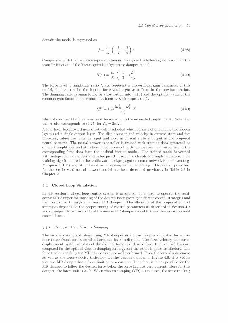
4.4 Closed-Loop Simulation 51
domain the model is expressed as
f =fmX
(−1
2+ i
2
π
)x (4.28)
Comparison with the frequency representation in (4.2) gives the following expression for thetransfer function of the linear equivalent hysteretic damper model:
H(ω) =fmX
(−1
2+ i
2
π
)(4.29)
The force level to amplitude ratio fm/X represent a proportional gain parameter of thismodel, similar to α for the friction force with negative stiffness in the previous section.The damping ratio is again found by substitution into (4.10) and the optimal value of thecommon gain factor is determined stationarity with respect to fm,
foptm = 1.24
(ω2∞ − ω2
0)
u20
X (4.30)
which shows that the force level must be scaled with the estimated amplitude X . Note thatthis results corresponds to (4.25) for fm = 2αX .
A four-layer feedforward neural network is adopted which consists of one input, two hiddenlayers and a single output layer. The displacement and velocity in current state and fivepreceding values are taken as input and force in current state is output in the proposedneural network. The neural network controller is trained with training data generated atdifferent amplitudes and at different frequencies of both the displacement response and thecorresponding force data from the optimal friction model. The trained model is verifiedwith independent data sets and subsequently used in a closed-loop implementation. Thetraining algorithm used in the feedforward backpropagation neural network is the Levenberg-Marquardt (LM) algorithm based on a least-square curve fitting. The design procedurefor the feedforward neural network model has been described previously in Table 2.3 inChapter 2.
4.4 Closed-Loop Simulation
In this section a closed-loop control system is presented. It is used to operate the semi-active MR damper for tracking of the desired force given by different control strategies andthen forwarded through an inverse MR damper. The efficiency of the proposed controlstrategies depends on the proper tuning of control parameters as described in Section 4.3and subsequently on the ability of the inverse MR damper model to track the desired optimalcontrol force.
4.4.1 Example: Pure Viscous Damping
The viscous damping strategy using MR damper in a closed loop is simulated for a five-floor shear frame structure with harmonic base excitation. The force-velocity and force-displacement hysteresis plots of the damper force and desired force from control laws arecompared for the optimal viscous damping strategy and the result is quite satisfactory. Theforce tracking task by the MR damper is quite well performed. From the force-displacementas well as the force-velocity trajectory for the viscous damper in Figure 4.6, it is visiblethat the MR damper has a force limit at zero current. Therefore, it is not possible for theMR damper to follow the desired force below the force limit at zero current. Here for thisdamper, the force limit is 24 N. When viscous damping (VD) is emulated, the force tracking

52 Control Strategies and Simulation
error is mainly given by the residual force at 0 A and the noise in the current due to theneural network based force tracking as seen from Figures 4.5(a,b). The structural dampingof the first excited mode is determined from the top floor displacement. The time history ofthe top floor displacement and damper displacement is shown in Figures 4.5 and 4.6. Theother control concepts are then tested in a simulation at the same excitation amplitude asin Figure 4.5(c,d). The viscous damping strategy is also applied directly to the structurewithout MR damper and the change in performance is compared.
Current,A
Time, S5 6 7 8 90
0.5
1
1.5
2force1force2
Force,
N
Time, S54 6 73
0
50
100
-50
-100
Damper
Displacement,
m
Time, S854 6 7
0
0.005
0.01
-0.005
-0.01 TopFloorDisplacement,m
Time, S854 6 7
0
0.05
-0.05
Figure 4.5: Current (a), Force comparison (b), Damper displacement (c), Top floordisplacement (d) (VD)
4.4.2 Example: Viscous Damping with Negative Stiffness
A negative stiffness component is added to the viscous part and then the optimal viscous pa-rameter is determined. As seen from Figure 4.8, the measured force-displacement trajectoryof viscous damping with negative stiffness (VDNS) is spiky. The spikes are triggered by theinitial very large increase of the desired force when the MR damper displacement turns itsdirection. The currents and the force tracking are shown in Figure 4.7. Force displacementand force velocity trajectories for actual and desired forces are shown in Figure 4.8. Thetime history for top floor and damper displacement is shown in Figure 4.7 , where it is clearlyvisible that introducing negative stiffness significantly reduces the top floor displacement.
4.4.3 Example: Frictional Damping with Negative Stiffness
Friction damping with negative stiffness is emulated. The actual force-displacement tra-jectories in the experiment and the simulation are not that noisy as viscous damping withnegative stiffness, which shows better structural damping and reduced top floor displace-ment. The currents and the force tracking are shown in Figure 4.9. The force-displacement

4.4 Closed-Loop Simulation 53
ActualForce,
N
Damper Displacement, m
50
100
-50
-100
0
0 0.005 0.01-0.005-0.01
Desired
Force,
N
Damper Displacement, m
50
100
-50
-100
0
0 0.005 0.01-0.005-0.01
ActualForce,
N
Damper velocity, m/s
50
100
-50
-100
0
0 0.05 0.1-0.05-0.1
Desired
Force,
N
Damper velocity, m/s
50
100
-50
-100
0
0 0.05 0.1-0.05-0.1
Figure 4.6: Force-displacement and force-velocity trajectories (VD)
Current,A
Time, S5 6 7 8 90
0.5
1
1.5
2force1force2
Force,
N
Time, S54 6 73
0
50
100
-50
-100
x 10−3
Damper
Displacement,
m
Time, S85
4
4
6
6 7
0
2
-2
-4
-6
TopFloorDisplacement,
m
Time, S854 6 7
0
0.05
-0.05
Figure 4.7: Current (a), Force comparison (b), Damper displacement (c), Top floordisplacement (d) (VDNS)
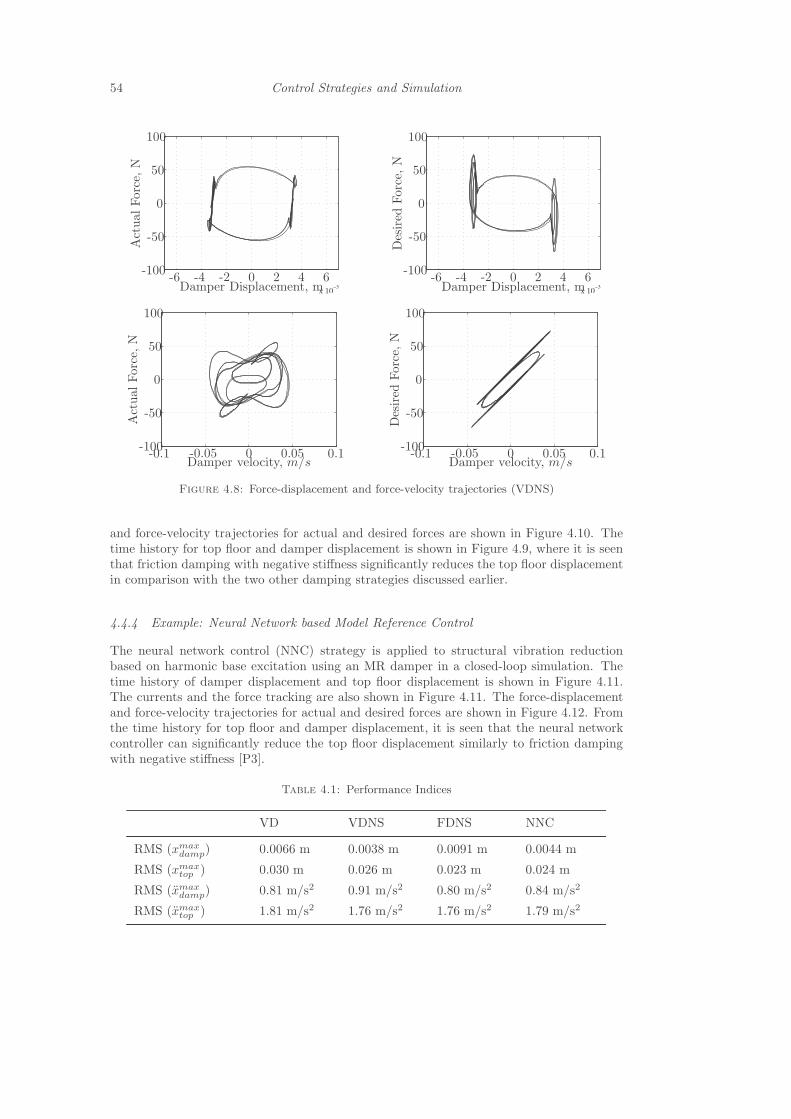
54 Control Strategies and Simulation
x 10−3
ActualForce,
N
Damper Displacement, m
50
100
-50
-1004 6
0
0 2-2-4-6x 10
−3
Desired
Force,
N
Damper Displacement, m
50
100
-50
-1004 6
0
0 2-2-4-6
ActualForce,
N
Damper velocity, m/s
50
100
-50
-100
0
0 0.05 0.1-0.05-0.1
Desired
Force,
N
Damper velocity, m/s
50
100
-50
-100
0
0 0.05 0.1-0.05-0.1
Figure 4.8: Force-displacement and force-velocity trajectories (VDNS)
and force-velocity trajectories for actual and desired forces are shown in Figure 4.10. Thetime history for top floor and damper displacement is shown in Figure 4.9, where it is seenthat friction damping with negative stiffness significantly reduces the top floor displacementin comparison with the two other damping strategies discussed earlier.
4.4.4 Example: Neural Network based Model Reference Control
The neural network control (NNC) strategy is applied to structural vibration reductionbased on harmonic base excitation using an MR damper in a closed-loop simulation. Thetime history of damper displacement and top floor displacement is shown in Figure 4.11.The currents and the force tracking are also shown in Figure 4.11. The force-displacementand force-velocity trajectories for actual and desired forces are shown in Figure 4.12. Fromthe time history for top floor and damper displacement, it is seen that the neural networkcontroller can significantly reduce the top floor displacement similarly to friction dampingwith negative stiffness [P3].
Table 4.1: Performance Indices
VD VDNS FDNS NNC
RMS (xmaxdamp) 0.0066 m 0.0038 m 0.0091 m 0.0044 m
RMS (xmaxtop ) 0.030 m 0.026 m 0.023 m 0.024 m
RMS (xmaxdamp) 0.81 m/s2 0.91 m/s2 0.80 m/s2 0.84 m/s2
RMS (xmaxtop ) 1.81 m/s2 1.76 m/s2 1.76 m/s2 1.79 m/s2

4.4 Closed-Loop Simulation 55
Current,A
Time, S5 6 7 8 90
0.5
1
1.5
2force1force2
Force,
N
Time, S54 6 73
0
50
100
-50
-100
Damper
Displacement,m
Time, S854 6 7
0
0.005
0.01
-0.005
-0.01TopFloorDisplacement,
m
Time, S854 6 7
0
0.05
-0.05
Figure 4.9: Current (a), Force comparison (b), Damper displacement (c), Top floordisplacement (d) (FDNS)
ActualForce,
N
Damper Displacement, m
50
100
-50
-100
0
0 0.005 0.01-0.005-0.01
Desired
Force,
N
Damper Displacement, m
50
100
-50
-100
0
0 0.005 0.01-0.005-0.01
−0.15 0.15
ActualForce,
N
Damper velocity, m/s
50
100
-50
-100
0
0 0.05 0.1-0.05-0.1 −0.15 0.15
Desired
Force,
N
Damper velocity, m/s
50
100
-50
-100
0
0 0.05 0.1-0.05-0.1
Figure 4.10: Force-displacement and force-velocity trajectories (FDNS)

56 Control Strategies and Simulation
Current,A
Time, S5 6 7 8 90
0.5
1
1.5
2force1force2
Force,
N
Time, S54 6 73
0
50
100
-50
-100
Damper
Displacement,
m
Time, S854 6 7
0
0.005
0.01
-0.005
-0.01 TopFloorDisplacement,m
Time, S854 6 7
0
0.05
-0.05
Figure 4.11: Current (a), Force comparison (b), Damper displacement (c), Top floordisplacement (d) (NNC)
ActualForce,
N
Damper Displacement, m
50
100
-50
-100
0
0 0.005 0.01-0.005-0.01
Desired
Force,
N
Damper Displacement, m
50
100
-50
-100
0
0 0.005 0.01-0.005-0.01
ActualForce,
N
Damper velocity, m/s
50
100
-50
-100
0
0 0.05 0.1-0.05-0.1
Desired
Force,
N
Damper velocity, m/s
50
100
-50
-100
0
0 0.05 0.1-0.05-0.1
Figure 4.12: Force-displacement and force-velocity trajectories (NNC)

4.5 Summary 57
4.5 Summary
The damping of a shear frame with five masses with controlled MR damper between groundplate and the first mass was investigated in a simulation. The tested control laws wereviscous damping, viscous damping with negative stiffness and optimal semi-active frictiondamping with negative stiffness and neural network based model reference control. Thecontrol laws were designed using a validated model of the shear frame. In the closed-loopsimulation, a neural network MR model is used for force tracking. Rms values of the peakdisplacement and peak acceleration of each cycle for top floor and damper location are takenas performance parameters. From the performance parameters chart in Table 4.1, it is clearlyvisible that introducing negative stiffness can make significant reduction in damper displace-ment and also in top floor displacement. The response of the top floor using semi-activeneural controller and friction damping with negative stiffness gives quite satisfactory resultscompared with pure viscous damping and pure viscous damping with negative stiffness. Asignificant improvement in acceleration is also observed but the acceleration contains somenoise.

Chapter 5
Experimental Implementation of Control Strategies
Survival of civil structures from excessive random vibration due to uncontrollable externalevents - due to natural hazards and otherwise - is very important where vibration controlof large flexible structures, such as shear frame buildings, is a great task in closed loopsituation. Some success of practical implementation of control laws to attain this goal hasbeen reported in the use of semi-active control devices as for instance magnetorheologicaldampers [99].
The following sections describe experimental implementation of semi-active control strategiesfor a shear frame with a controlled magnetorheological (MR) damper mounted betweenground and first floor in order to mitigate the fundamental bending mode. Some linearcontrol strategies, for example, optimal viscous damping, clipped viscous damping withnegative and positive stiffness and also nonlinear control strategies, for example, optimalfriction damping with negative stiffness are implemented. MR damper is a semi-activedevice and control law can not give direct command to MR damper to produce desiredforce. For semi active control strategy requires a feed forward mechanism which will produceappropriate current from the desired force value from controller output and feed the currentinto the MR damper to generate proper force value. This mechanism is also called as forcetracking mechanism. The force tracking is solved with a novel neural network model of theMR damper that takes the absolute values of damper velocity and desired force as inputsbecause the outputted desired current is a positive quantity [P1]. The force tracking isimproved by a low-pass filter to reduce the noise in the desired current and a switch thattruncates the desired current to zero, if the desired force is smaller than the residual forceat 0 A [P2]. The measured and simulated control forces still show a spiky behaviour dueto the fairly large sensitivity of the neural network to slightly noisy inputs. However, themeasured and simulated structural damping ratios correspond well to the expected values.This indicates that the mean stiffness and mean energy dissipation of the control force mainlydetermine the structural damping [P2]. Negative stiffness is introduced into the design ofcontrol laws. To demonstrate the significance of the negative stiffness, positive stiffness isalso introduced with viscous damping. The closed loop implementation of the control lawson real structure also demonstrate the significant improvement in structural damping dueto inclusion of negative stiffness [P2].
5.1 Experimental Setup
The experimental setup consists of a hydraulic cylinder driving a shaking table on which a5 DOF system is mounted. The experimental setup at the EMPA structural laboratory isshown in Figure 5.1. The housing of the MR damper is fixed to the shaking table and theMR damper rod applies the semi-active control force to the first mass of the 5 DOF system.This situation is equivalent to a 5 DOF system with controllable damper that mitigatesthe relative motion between ground and first floor. The MR damper under considerationis a rotational type with approximately 22 N residual force at 0 A and 300 N at maximumcurrent of 4 A [56].
58
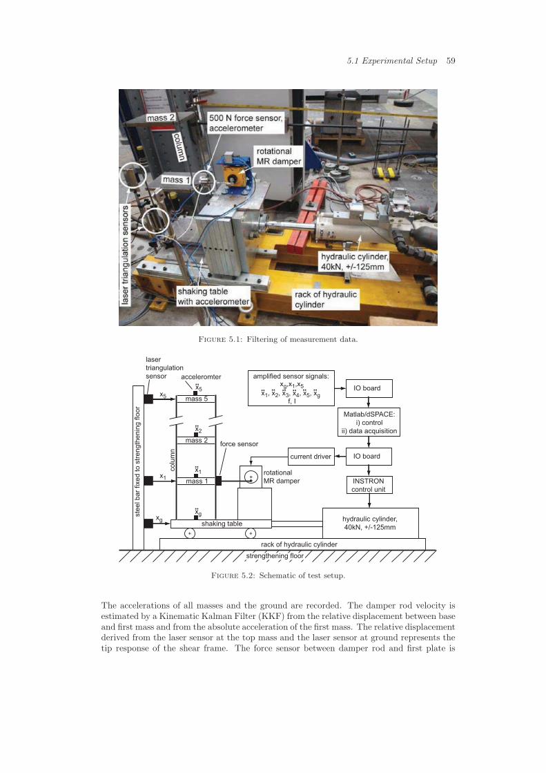
5.1 Experimental Setup 59
Figure 5.1: Filtering of measurement data.
mass 5
mass 2
mass 1
x5x5
x1
xg
..
x1..
x2..
xg..
rotational
MR damper+
amplified sensor signals:
IO board
Matlab/dSPACE:
i) control
ii) data acquisition
IO boardcurrent driver
INSTRON
control unit
xg,x1,x5
f, I
shaking table
rack of hydraulic cylinder
hydraulic cylinder,
40kN, +/-125mm
strengthening floor
laser
triangulation
sensor
ste
el b
ar
fixe
d t
o s
tre
ng
the
nin
g f
loo
r
acceleromter
force sensor
co
lum
n
++
x1, x2, x3, x4, x5, xg.. .. .. .. .. ..
Figure 5.2: Schematic of test setup.
The accelerations of all masses and the ground are recorded. The damper rod velocity isestimated by a Kinematic Kalman Filter (KKF) from the relative displacement between baseand first mass and from the absolute acceleration of the first mass. The relative displacementderived from the laser sensor at the top mass and the laser sensor at ground represents thetip response of the shear frame. The force sensor between damper rod and first plate is

60 Experimental Implementation of Control Strategies
installed in order to measure the force tracking error but it is not used as force feedback.The schematic of the test setup is shown in Figure 5.2.
The controller is programmed in Matlab/dSPACE which is also used for the data acquisition.The control algorithm outputs the desired control force at a sampling frequency of 500 Hz.A neural network based inverse MR damper model is used to determine the desired currentin real-time. The desired current is converted into a command voltage that is outputted bythe IO board and is fed to the current driver of type KEPCO that guarantees negligiblysmall tracking error of the MR damper current. The Matlab/Simulink file of the controlleris also used to output the command voltage of the INSTRON control unit that controls thehydraulic cylinder displacement.
5.2 Velocity Estimation Using Kinematic Kalman Filter
The inverse neural network model for the MR damper depends partly on proper velocitymeasurement to track the desired force. The velocity cannot be measured directly. The onlyway to measure velocity is taking a differentiation of measured displacement data or takingmeasured acceleration data into consideration. However, including a differentiator to thesystem adds noise, while accelerations are inherently noisy and an integrator furthermoreintroduces a phase delay to the resulting signal. Therefore, a simple but effective methodis needed for fusing displacement and acceleration data to derive velocity. The KinematicKalman Filter (KKF) is a very effective tool for simple and robust estimation of veloc-ity [98]. KKF does not depend on plant parameters as in model based Kalman filters. Ifthe displacement and acceleration are both measured, the system equation and the KKFestimation model are designed to fuse displacement and acceleration to estimate velocity.The system model for Kinematic Kalman Filter is given as
[x1
x2
]=
[0 10 0
] [x1
x2
]+
[01
] [am + wa
]
y = xm + wx
(5.1)
The output equation can then be represented as
y =[1 0
] [x1
x2
]+ wx (5.2)
The two-state variables are the displacement x1 = x and the velocity x2 = x of the sys-tem. wa and wx are accelerometer measurement noise and displacement measurement noise,respectively. The KKF is obtained as
[˙x1
˙x2
]=
[0 10 0
] [x1
x2
]+
[kl
] [y − x1
](5.3)
where k and l are filter gains. From the KKF the predicted displacement is x1 and thepredicted velocity is x2. The advantage of KKF is that it is model parameter independent.
5.3 Closed-Loop Model Design in Matlab/Simulink
As seen from Figure 5.3, the model is extended by a switch and analogue low-pass But-terworth filter. The switch outputs Ides(k) = 0A if the absolute value of the desired force|fdes(k)| is smaller than the residual force at 0 A of the MR damper under consideration.The application of this practical knowledge reduces the control force tracking error dueto modelling errors at small forces. The Butterworth filter with cutoff frequency 60 Hz isincluded to reduce the noise in the desired current. The noise has mainly two sources:

5.3 Closed-Loop Model Design in Matlab/Simulink 61
zero currentif abs(f_des)<18N
f _act
x_dot_dot_g
x1
x_dot_1
Validated Shear Frame Model
f _des_abs
x_dot_1_abs
I_des_NN
Validated NeuralNetwork of Inverse
Behaviour
I_actx_dot_1
f _act
Validated Bouc WenModel of Forward
MR Damper Behaviour
butter
Low Pass Filterwith Cutoff
Frequency 60Hz
30
x_1
x_dot_1f _des_unclipped
Control Law
0
Clock
f _des_unclipped
x_dot_1f _des
Clipping
time x_dot_dot_g
Base Excitation
|u|
|u|
MR Damper
Model of Real Plant:
MR Damper with Shear Frame on Shaking Table
Entire Controller as programmed in Matlab/dSPACE
Current Driver KEPCO
I_des=I_act
Figure 5.3: Matlab/Simulink model of closed loop system.
� One is the high frequencies in the damper velocity that are generated when fdes cannotbe tracked because fdes is larger than the residual force at 0 A. This leads to clampingeffects of the shear frame in the damper position. When the force is larger than theresidual force value at 0 A, the desired force fdes can be tracked and the MR damperstarts to work again. The sudden change between locked and smoothly operating MRdamper induces the high-frequency signal parts in the damper velocity. This noisesource exists in both the simulations and the experiments.
� Another source is the measurement noise, which only exists in the experimental data.The input of the feed forward part are the measured damper velocity x and the desireddamper force fdes, which both include measurement noise and thereby evoke a noisydesired damper current Ides.
In order to compare the simulated and measured force tracking and damping of the 5 DOFsystem, the simulations and the measurements of the closed loop are performed with anidentical controller. The controller includes the subsystems control law, clipping, validatedneural network of inverse MR damper behaviour, switch and low-pass filter with cut-offFrequency 60Hz as depicted in Figure 5.3 which is programmed in Matlab/ dSPACE. Thecontroller runs at a sampling frequency of 200 Hz, which is the same as used to train theneural network [P1, P2]. The simulation of the closed loop assumes zero current trackingerror, i.e. the desired and the actual currents are equal (Ides = Iact). At the test setup,the current driver (KEPCO) is used to guarantee a negligibly small current tracking error,i.e. Ides ≈ Iact. The MR damper is simulated with a validated Bouc-Wen model of the MRdamper under consideration. The simulated shear frame model is given in Chapter 3. In thesimulations, the shear frame structure is excited by the actual measured base accelerationrecord xg = xmeas
g .

62 Experimental Implementation of Control Strategies
13.6 13.8 14 14.2 14.4 14.6 14.8 15 15.2−100
−80
−60
−40
−20
0
20
40
60
80
100fo
rce [N
]
desired forceactual force
time [s]
measured, almost steady state, VD
0
0.2
0.4
0.6
0.8
1
1.2
1.4
1.6
1.8
13.6 13.8 14 14.2 14.4 14.6 14.8 15 15.2
curr
ent [A
]
time [s]
actual current(b)(a)
13.4 13.6 13.8 14 14.2 14.4 14.6 14.8 15 15.2−100
−80
−60
−40
−20
0
20
40
60
80
100
13.4 13.6 13.8 14 14.2 14.4 14.6 14.8 15 15.2
0
0.2
0.4
0.6
0.8
1
1.2
1.4
1.6
1.8
curr
ent [A
]
forc
e [N
]
desired forceactual force
time [s]
simulated, steady state, VD
measured, almost steady state, VD
simulated, steady state, VD
actual current(d)(c)
force at 0 A
force at 0 A
Figure 5.4: Measured (a,b) and simulated (c,d) force tracking with NN based MRdamper model.
5.4 Force Tracking
The force tracking error is depicted in Figure 5.4 for viscous damping (VD) and the maximumviscous force of approximately 60 N which is a typical value for the first mode of the shearframe under consideration. The force tracking error in the experiment is slightly larger thanin the simulation since the measurement noise in the collocated velocity produces a fairlynoisy desired force which generates a noisy current as shown in Figure 5.4(b). The actualforce is not so noisy as the applied current because the MR damper behaves similarly to alow-pass filter that mitigates these spikes to some extent. It is seen from Figures 5.4(a,c)that the resulting force tracking error in experiment and simulation is acceptably small.Both time histories show the regions of the residual force that constrains the force tracking.Here, zero applied current is the best choice in order to minimise the force tracking error.
5.5 Experimental and Numerical Simulation
Section 5.4 shows the measured and simulated force tracking error due to the inverse neu-ral network approach that is used as model-based feedforward. This section presents themeasured and simulated force displacement trajectories, the force-velocity trajectories andthe free decay responses of the 5 DOF system resulting from different control concepts: Vis-cous damping (VD), viscous damping with positive stiffness (VDPS), viscous damping withnegative stiffness (VDNS) and friction damping with negative stiffness (FDNS). In order todemonstrate the negative impact of positive stiffness on the damping of the 5 DOF, alsoclipped viscous damping with positive stiffness is tested. The desired force-displacement

5.5 Experimental and Numerical Simulation 63
trajectories are shown in Figures 5.5.
fdes
x1-rel
fdes
x1-rel
fdes
x1-rel
(a) (c) (d)
kdes kdes
fdes
x1-rel
(b)
kdes
Figure 5.5: Desired force displacement trajectories: VD (a), VDPS (b)VDNS (c),FDNS (d).
5.5.1 Pure Viscous Damping
When viscous damping (VD) is emulated, the force tracking error is mainly given by theresidual force at 0 A and the noise in the current due to the neural network based forcetracking shown in Figure 5.6. The structural damping of the first excited mode is determinedfrom the top floor displacement x5. Due to the fairly large damper position of 1/11 ofthe wave length of the first mode, the resulting structural damping is large. Therefore,the number of local peaks with non-zero MR damper current is small which explains thevariation of the point-to-point damping ratio shown in Figure 5.7. Thus, the point-to-pointdamping ratio values are averaged by the exponential fit from which the mean damping ratioζ is obtained. The values are shown in Table. 5.1. Only the local peaks with non-zero currentduring their corresponding half period time are taken into consideration for the assessmentbecause these peaks represent the decay response due to controlled damping. The dampingof the subsequent peaks is determined by the residual force of the MR damper that cannotbe controlled as such. The time history of the displacement during this subsequent partshows an almost triangular shape which indicates predominant friction damping due to thedamper ceilings and bearings. As Table. 5.1 shows, the structural damping that is achievedon the real structure is a little bit smaller than the one obtained in the simulation whichmight be the effect of increased force tracking error on the real structure with the real MRdamper.
In addition to the mean damping ratio, the damping performance of the tested controlconcepts is also assessed by the root mean square (rms) of the steady state response ofthe tip displacement for constant excitation amplitude (Table 5.1). In order to be able tocompare the rms values of the tests and the simulations, the excitation amplitude of baseacceleration xg in the simulation is adjusted such that the rms(x5) is equal for simulationsand experiments associated with viscous damping (VD). The other control concepts are thentested in a simulation at the same excitation amplitude. The rms is determined for:
� The displacement of the top floor, which illustrates the damping performance.
� The displacement of the first floor, which indicates the potential softening due tonegative stiffness.
� The acceleration of the top floor, which also identifies the overall damping.
� The acceleration of the first floor, which gives a direct measure for the high-frequencycontent and thereby the spill-over effect.
The rms values resulting from VD are the benchmark and the rms values due to the othertested control concepts can then be compared to this benchmark. Measured and simulatedmean damping ratios and steady state responses are determined for constant excitation

64 Experimental Implementation of Control Strategies
Table 5.1: Comparison between Measured and Simulated Performance
control law VD Clipped VDPS Clipped VDNS FDNS
tuning c = 650 Nm/s c = 400 Nm/s c = 250 Nm/s α=3000N/m
k = +2500 N/m k = -4000 N/m
measured
ζ [%] 11.8 9.0 approx. 22 approx. 26
rms(x5) [mm] 24.3 23.03 15.5 11.2
rms(x1) [mm] 6.6 6.7 4.9 3.5
rms(x5) [mm] 1.81 1.84 1.25 1.02
rms(x1) [mm] 0.87 1.27 1.02 0.94
simulated
ζ [%] 13.4 9.6 approx. 30 approx. 30
rms(x5) [mm] 24.3 35.4 13.8 13.6
rms(x1) [mm] 6.1 8.8 6.3 5.5
rms(x5) [mm] 1.60 2.28 0.98 1.16
rms(x1) [mm] 0.64 0.93 1.40 1.36
amplitude and actual resonance frequency of the excited first mode where the amplitude ofxg is such that the measured rms(x5) is equal to the simulated rms(x5).
5.5.2 Viscous Damping with Positive Stiffness
Both the measurements and the simulations of clipped viscous damping with positive stiff-ness (VDPS) show the typical kink in the force-displacement trajectory due to the clipping,see Figure 5.8(a,c). The measured force follows approximately the desired force except wherethe tracking is constrained by the residual force at 0 A. As expected from the theory, thepositive stiffness evokes smaller damping in the structure than pure VD, see Table 5.1. Thedecreased damping leads to larger rms values in the simulations. The experiments approxi-mately show the same rms values as for VD. This result can be explained by the increasedforce tracking error due to the increased residual force when clipped VDPS is emulated.Figure 5.8(a) shows a residual force of approximately 30 N, whereas Fig. 5.7(b) points out avalue of approximately 22 N when VD is emulated. In the case of clipped VDPS, the desiredforce reaches its maximum at displacement extreme. Then, the MR damper current is largewhich generates large remanent magnetisation in the MR fluid and also in all ferromagneticdamper parts. When the desired force crosses the x-axis in Figure 5.8(a), the desired forceis zero and increases with increasing damper displacement step by step. The high remanentmagnetisation from the force peak before makes it impossible to track a very small force.It even leads to an increased residual force at 0 A compared to e.g. VD, where the currentis lowered step by step when the damper displacement reaches its extreme and the effect ofthe remanent magnetisation on the residual force at 0 A is thus smaller. The higher residualforce in case of clipped VDPS changes the shape of the actual force-displacement trajectory

5.5 Experimental and Numerical Simulation 65
−15 −10 −5 0 5 10 15
−100
−50
0
50
100
displacement [mm]
forc
e [N
]
desired forceactual force
measured, almost steady state, VD
−0.15 −0.1 −0.05 0 0.05 0.1 0.15
−100
−50
0
50
100
velocity [m/s]
desired forceactual force
forc
e [N
]
−10 −5 0 5 10−80
−60
−40
−20
0
20
40
60
80
displacement [mm]
forc
e [N
]
desired forceactual force
−0.1 −0.05 0 0.05 0.1−80
−60
−40
−20
0
20
40
60
80
velocity [m/s]
desired forceactual force
forc
e [N
]
simulated, steady state, VDsimulated, steady state, VD
(a) (b)
(c) (d)
measured, almost steady state, VD
force at 0 A
force at 0 A
force at 0 A (18 N)
force at 0 A
force at 0 A (22 N)
force at 0 A
force at 0 A
force at 0 A
Figure 5.6: Measured and simulated control forces due to viscous damping.
19 20 21 22 23−50
−40
−30
−20
−10
0
10
20
30
40
50
time [s]
measured free decay test, VD
ζ [%
]
10
5
0
local maxima
point-to-point ζexponential fit
current 10 [A]
x5 [mm].
free decay
x5 [m
m]
19 20 21 22 23−50
−40
−30
−20
−10
0
10
20
30
40
50simulated free decay test, VD
ζ [%
]
10
0
local maxima
point-to-point ζexponential fit
current 10 [A]
x5 [mm].
x5 [m
m]
5
time [s]
free decay
(a) (b)
Figure 5.7: Measured and simulated free decay tests due to viscous damping.
to almost pure friction damping with negligibly small positive stiffness. The almost non-existent positive stiffness explains why the rms values due to VD and clipped VDPS are soclose in the experiments.
5.5.3 Viscous Damping with Negative Stiffness
As is seen from Figure 5.9 (a), the measured force-displacement trajectory of clipped VDNSis very spiky. The spikes are triggered by the initial very large increase of the desired forcewhen the MR damper displacement turns its direction. Then, the model-based feed forward
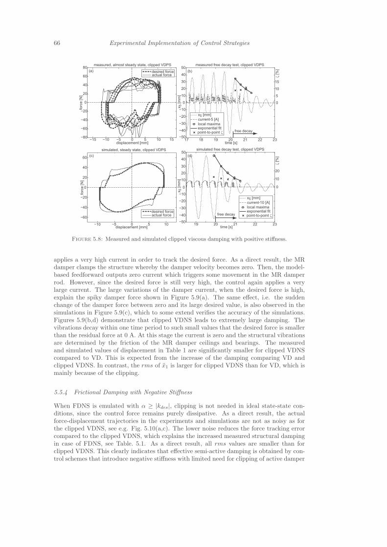
66 Experimental Implementation of Control Strategies
−15 −10 −5 0 5 10 15−80
−60
−40
−20
0
20
40
60
80
displacement [mm]
measured, almost steady state, clipped VDPS
desired forceactual force
forc
e [N
]
17 18 19 21 22 23−50
−40
−30
−20
−10
0
10
20
30
40
50
time [s]
ζ [%
]
10
15
0
local maxima
point-to-point ζexponential fit
current 5 [A]
x5 [mm].
free decay
x5 [m
m] 5
−10 −5 0 5 10
−60
−40
−20
0
20
40
60
simulated, steady state, clipped VDPS
displacement [mm]
desired forceactual force
forc
e [N
]
19 20 21 22 23
−40
−30
−20
−10
0
10
20
30
40
time [s]
ζ [%
]
10
20
0
local maxima
point-to-point ζexponential fit
current 10 [A]
x5 [mm].
free decay
x5 [m
m]
50
−50
20
(a) (b)
(c) (d)
measured free decay test, clipped VDPS
simulated free decay test, clipped VDPS
Figure 5.8: Measured and simulated clipped viscous damping with positive stiffness.
applies a very high current in order to track the desired force. As a direct result, the MRdamper clamps the structure whereby the damper velocity becomes zero. Then, the model-based feedforward outputs zero current which triggers some movement in the MR damperrod. However, since the desired force is still very high, the control again applies a verylarge current. The large variations of the damper current, when the desired force is high,explain the spiky damper force shown in Figure 5.9(a). The same effect, i.e. the suddenchange of the damper force between zero and its large desired value, is also observed in thesimulations in Figure 5.9(c), which to some extend verifies the accuracy of the simulations.Figures 5.9(b,d) demonstrate that clipped VDNS leads to extremely large damping. Thevibrations decay within one time period to such small values that the desired force is smallerthan the residual force at 0 A. At this stage the current is zero and the structural vibrationsare determined by the friction of the MR damper ceilings and bearings. The measuredand simulated values of displacement in Table 1 are significantly smaller for clipped VDNScompared to VD. This is expected from the increase of the damping comparing VD andclipped VDNS. In contrast, the rms of x1 is larger for clipped VDNS than for VD, which ismainly because of the clipping.
5.5.4 Frictional Damping with Negative Stiffness
When FDNS is emulated with α ≥ |kdes|, clipping is not needed in ideal state-state con-ditions, since the control force remains purely dissipative. As a direct result, the actualforce-displacement trajectories in the experiments and simulations are not as noisy as forthe clipped VDNS, see e.g. Fig. 5.10(a,c). The lower noise reduces the force tracking errorcompared to the clipped VDNS, which explains the increased measured structural dampingin case of FDNS, see Table. 5.1. As a direct result, all rms values are smaller than forclipped VDNS. This clearly indicates that effective semi-active damping is obtained by con-trol schemes that introduce negative stiffness with limited need for clipping of active damper

5.5 Experimental and Numerical Simulation 67
−15 −10 −5 0 5 10 15−80
−60
−40
−20
0
20
40
60
80
displacement [mm]
forc
e [N
]
19 20 21 22 23−40
−30
−20
−10
0
10
20
30
40
time [s]
ζ [%
]
10
30
40
0
local maxima
point-to-point ζexponential fit
current 10 [A]
x5 [mm].
free decay
x5 [m
m]
17 18 19 21 22 23−50
−40
−30
−20
−10
0
10
20
30
40
50
time [s]
ζ [%
]
10
20
0
local maxima
point-to-point ζexponential fit
current 5 [A]x5 [mm]
.
free decay
x5 [m
m]
20−15 −10 5 10 15−150
−100
−50
0
50
100
150
−5 0displacement [mm]
desired forceactual force
forc
e [N
]
desired forceactual force
measured, almost steady state, clipped VDNS
simulated, steady state, clipped VDNS
(a) (b)
(c) (d)
measured free decay test, clipped VDNS
simulated free decay test, clipped VDNS
Figure 5.9: Measured and simulated clipped viscous damping with negative stiffness.
forces.
−15 −10 −5 0 5 10 15−150
−100
−50
0
50
100
150
displacement [mm]
forc
e [N
]
desired forceactual force
17 18 19 21 22 23−50
−40
−30
−20
−10
0
10
20
30
40
50
time [s]
ζ [%
]
10
20
0
local maxima
point-to-point ζexponential fit
current 5 [A]
x5 [mm].
free decay
x5 [m
m]
19 20 21 22 23−50
−40
−30
−20
−10
0
10
20
30
40
50
time [s]
ζ [%
]
10
20
30
0
local maxima
point-to-point ζexponential fit
current 10 [A]
x5 [mm].
free decay
x5 [m
m]
displacement [mm]
forc
e [N
]
desired forceactual force
measured, almost steady state, FDNS
simulated, steady state, FDNS
(a) (b)
(c) (d)
measured free decay test, FDNS
simulated free decay test, FDNS
−30 −20 −10 0 10 20 30
−100
−50
0
50
100
Figure 5.10: Measured and simulated friction damping with negative stiffness.
68 Experimental Implementation of Control Strategies
5.6 Summary
The damping of a shear frame with five masses with controlled MR damper between groundplate and first mass was investigated in simulation and experiments. The tested controllaws were viscous damping, clipped viscous damping with negative and positive stiffnessand optimal semi-active friction damping with negative stiffness. The control laws weredesigned using a validated model of the shear frame. A novel approach of a validated neuralnetwork model of the inverse MR damper behaviour was used to track the desired controlforce. Since the neural network output, i.e. the desired MR damper current, is very sensitiveto measurement noise in the measured damper velocity input, the neural network outputwas fed through a low-pass filter. In addition, a switch was added to set the outputteddesired current to zero if the desired force was smaller than the residual force of the MRdamper under consideration. The entire controller included real-time processing of themeasured damper displacement and acceleration, real-time calculation of the four testedcontrol laws and real-time calculation of the neural network output and its extensions. Theentire controller was implemented in Matlab/dSPACE at a sampling frequency of 500 Hz.Despite the two extensions of the neural network, i.e. the low-pass filter and the switch,the actual MR damper force was still spiky. Nevertheless, the measured structural dampingagreed well with the simulated values. This is explained by the fact that the mean stiffnessand energy dissipation of the control force which were tracked fairly accurately, except whenthe desired force was smaller than the residual force at 0 A, mainly determined the resultingstructural damping. Thus, the neural network method represents a tool with which theinverse MR damper behaviour can be modelled directly in order to track the desired forcein real-time with sufficiently large accuracy without feedback from a force sensor.

Chapter 6
Applications to Benchmark Problems
In recent years, several control strategies have been developed and studied on differentbuildings for different dynamic loads. Some of the control strategies have been designedand implemented for real structures like cables or building structures or bridges. However,due to experimental limitations, it is hardly possible to implement the control laws on thesame building with the same load. Thus, the concept of benchmark problems has come intothe picture to compare the various control laws on the same building structure and for thesame dynamic load [38, 104]. Based on realistic full-scale buildings, two structural controlbenchmark problems have been identified for earthquake [38, 39] and wind excitations [40].
For the last decades, several design solutions have been developed and implemented forearthquake mitigation of high-rise buildings. In particular, base-isolation is an effective androbust method for reducing structural response due to earthquake excitation. The base-isolation technique consists of the installation of mechanisms that decouple the structureand its content from the earthquake induced ground motion, especially in the frequencyrange where the building is most affected. Base-isolation is designed to avoid potentialdamage in a cost-effective manner to both the structure and its content by reducing inter-floor drifts as well as floor accelerations. Successful base-isolation of a particular structurestrongly depends on the choice of isolator devices. The most commonly used types areelastomeric bearings, lead-rubber-bearings and friction pendulum bearings. Details aboutbase-isolation can be found in [100]. Adding supplemental damping to a structure via thebase can help reduce the response of the building and especially reduce the base displace-ment. However, the addition of damping to minimise base displacements may increaseboth internal deformation and absolute accelerations of the superstructure. The additionaldamping is provided by installing either passive control devices, active control devices orsemi-active control devices on the base-isolated building. The magnetorheological damperis commonly used device for robust semi-active control in connection with base isolationand earthquake excitation. Several semi-active control methods have been investigated forbase-isolated structures [101] - [107] and for wind excited structures [108] - [110].
This chapter first describes the implementation of different control strategies for a seismicallyexcited base-isolated building mounted on rubber bearings using MR dampers. Benchmarkproblems are slightly modified for studying semi-active control strategies for buildings excitedto earthquake loadings. The benchmark problem for a base-isolated building is similar to anexisting eight-floor building in the earthquake prone Los Angeles region. It is is proposedin [38] and is formulated in association with the ASCE structural control committee. In itsbasic version it is capable of incorporating three different kinds of base-isolation systems.Moreover, a sample controller design for the benchmark problem is evaluated in [39]. Thedetails of applied control strategies for this benchmark problem have already been discussedin Chapter 4 and also in [P2, P4]. The three types of control strategies are: the pureviscous damping (VD), the viscous damping with negative stiffness (VDNS) and the frictiondamping with negative stiffness (FDNS). Two MR dampers are acting on the structure atthe mass center of the base slab, working in the two planar direction at the base. Theparameter calibration of the control strategies are determined by the method following thetwo-component reduction technique of Main and Krenk [29]. The performance of the control
69

70 Applications to Benchmark Problems
Table 6.1: Bingham Model Parametrs
fa 100 kN fb 75.0 kN/A
ca 81.0 kN s/m cb 90.0 kN s/m/V
methods is assessed in terms of nine performance indices, which are defined in benchmarkproblems.
The second part of this chapter describes the implementation of the developed control strate-gies for a wind excited building. The wind-excited benchmark building is a 76-floor, 306 mtall, concrete office tower, proposed for the city of Melbourne, Australia. The building istall and slender with a height-to-width ratio of 7.3. Hence, it is wind sensitive, and windtunnel tests have been conducted for a building model at the University of Sydney. Theresults of the across-wind data are provided for the analysis of the benchmark problem, anda number of performance criteria are evaluated based on this benchmark problem.
6.1 Magnetorheological Damper: Forward and Inverse Model
For the benchmark problem, two large scale MR damper of 1000 kN are considered. Theobjective of the benchmark problem is to show effectiveness of negative stiffness on severalsemi-active control approaches. For that reason a simple MR damper model based onbingham plasticity theory is considered in the benchmark study [13, 35].
The governing equation for the damper force f predicted by the Bingham model is expressedas
f = [fa + fbI]sign[x] + [ca + cbI]x (6.1)
The parameters of the Bingham model are given in Table 6.1. The Bingham model is alsoused in [P4] for inverse MR damper design. But in this case, neural network based inverseMr damper is developed based on the methods discussed in [P1]. The Bingham model hastwo inputs i.e., current and velocity and one output force. The generated force at differentconstant current level (2 A,4 A, 6 A) is shown in Figure 6.1(a). The training set for NNmodel here is modified so that it can work with transient behaviour. The training set consistsof sinusoidal, triangular, constant step and gaussian white noise (GWN) displacement inputsand also current input. The validation of inverse neural model of the Bingham model forsinusoidal displacement (0.1 m and 3.0 Hz) and sinusoidal current input (5 A and 3.0 Hz)is shown in Figure 6.1(b). The inverse neural network modeling and its training procedureare already discussed in Chapter 2. From Figure 6.1(b), it is visible that the inverse neuralnetwork can predict the current accurately though it generates some spiky current due tosmall modelling error. But this can be removed by proper filtering [P1]. So the validatedmodel is used as feed forward component for force tracking in the control design in both thebenchmark problems.
6.2 Seismically Excited Base-Isolated Benchmark Building
The performance of the control strategies are initially evaluated for the base-isolation struc-ture exposed to the El Centro earthquake problem. First the model is introduced and thenthe performance indices are used to compare the control strategies and evaluated based onthe damper performance. The results are also compared to the active LQG sample controllerof the benchmark problem.

6.2 Seismically Excited Base-Isolated Benchmark Building 71
6.2.1 Structural Model and Evaluation Criteria
The benchmark structure has been developed for the base-isolated benchmark problem de-fined in [38]. The detailed modelling of the benchmark structure is given in Appendix. A.The base-isolated building has eight floors with an average floor height of 4.04m, a widthof 54.3m and a length of 82.4 m. The floor plan is L-shaped for the first six floors andrectangularly shaped for the two top floors. The schematic view of the floor plan and thebuilding is presented in Figures 6.2(a,b).
The benchmark building has steel-braced frames with the superstructure bracing located atthe building perimeter. The superstructure is supported on a reinforced concrete base slab,and metal decking and a grid of steel beams support all concrete floor slabs. The elevationview with the base isolation system and the control device is shown in Figure 6.2(c). A totalnumber of 92 isolation bearings are used in the present problem, and they are designed assimple linear elastic rubber bearings, whereby a fully linear isolation system can be assumed
20 25 30 35−1000
−500
0
500
1000
Force,
kN
Time, S10 15 200
2
4
6
8
10
Current,A
Time, S
simulatedNN model
Figure 6.1: Force diagram for MR damper (a) and Inverse model validation (b)
Figure 6.2: Schematic diagram of the benchmark building [38].

72 Applications to Benchmark Problems
0 5 10 15 20 25 30
−5
0
5
El Centro, FN
Time [s]
Acc
. [m
/s2]
0 5 10 15 20 25 30
−5
0
5
El Centro, FP
Time [s]
Acc
. [m
/s2 ]
Figure 6.3: earthquake acceleration
in the analysis. The superstructure is modelled as a three-dimensional linear elastic systemwith lateral torsional behaviour, and the floor slabs as well as the base are assumed to berigid. Each floor plan and the isolation system is modelled using three degrees of freedomlocated at the center of mass of each floor. They are the two horizontal displacementsand the torsional rotation of each slap/floor. Thus, the superstructure itself has a total of24 DOFs, which yields 24 vibration modes in a fixed-base situation. When including themotion of the base slab, which is supported by the base-isolation system, the total numberof DOFs increase to 27. Details of the mathematical modelling of the benchmark structureare discussed in [38]. In the following, when the structure is denoted as uncontrolled itmeans that no supplemental control devices are attached. This configuration is used as areference case when evaluating the performance of the control strategies operating on thebase-isolation system.
In the performance evaluation criteria the structural response quantities are normalised bytheir corresponding uncontrolled values. If the uncontrolled values do not exist, e.g. thecontrol force, the values are not normalized. The performance of the controllers is shownin Table 6.3 by the performance indices J1 to J9 which are defined in Appendix B. Thestructural model is discussed in details in Appendix A, and the detailed definition anddescription of the various performance indices for the evaluation of the proposed controlstrategies are summarized in Appendix B.
6.2.2 Numerical Simulation
The time domain dynamic analysis has been conducted for the computational structuralmodel developed in MATLAB of a base-isolated benchmark building to investigate thecomparative performance of the collocated control laws on the structural response of thebenchmark building under El-Centro earthquake ground motion. The two horizontal com-ponents of all the earthquakes are designated as fault-normal (F-N) and fault parallel (F-P),as shown in Figure 6.3. The earthquake time history of the El-Centro earthquake recordhas been considered with a time step of 0.001 s for the first 30 s in the simulation. The
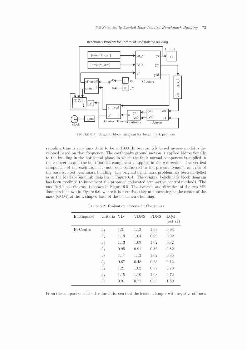
6.2 Seismically Excited Base-Isolated Benchmark Building 73
Structure
ye
ym
ycd
ug_x
ug_y
yf
ye
J1 to J8
[time’,Y_dir’]
[time’,X_dir’]
ym
sig_1
ym
yf
ys1
ys2
Sensors
ys1
ys2uu
ycdf
yf
f
on/offyf
switch
1
0 off
on
yf
ye
on/o
ff
t_out
clockControllerControl Devices
Benchmark Problem for Control of Base Isolated Building
yf
Figure 6.4: Original block diagram for benchmark problem
sampling time is very important to be at 1000 Hz because NN based inverse model is de-veloped based on that frequency. The earthquake ground motion is applied bidirectionallyto the building in the horizontal plane, in which the fault normal component is applied inthe x-direction and the fault parallel component is applied in the y-direction. The verticalcomponent of the excitation has not been considered in the present dynamic analysis ofthe base-isolated benchmark building. The original benchmark problem has been modelledas in the Matlab/Simulink diagram in Figure 6.4. The original benchmark block diagramhas been modified to implement the proposed collocated semi-active control methods. Themodified block diagram is shown in Figure 6.5. The location and direction of the two MRdampers is shown in Figure 6.6, where it is seen that they are operating at the center of themass (COM) of the L-shaped base of the benchmark building.
Table 6.2: Evaluation Criteria for Controllers
Earthquake Criteria VD VDNS FDNS LQG(active)
El-Centro J1 1.31 1.13 1.09 0.93
J2 1.19 1.04 0.99 0.92
J3 1.13 1.09 1.02 0.82
J4 0.95 0.91 0.86 0.82
J5 1.17 1.12 1.02 0.85
J6 0.67 0.48 0.33 0.12
J7 1.21 1.02 0.92 0.78
J8 1.15 1.10 1.03 0.72
J9 0.91 0.77 0.65 1.89
From the comparison of the J-values it is seen that the friction damper with negative stiffness

74 Applications to Benchmark Problems
Structure
ye
ym
ycd
ug_x
ug_y
yf
ye
J1 to J8
[time’,Y_dir’]
[time’,X_dir’]
ycd
ycdvv
ycdf
yf
f
on/offyf
switch
1
0 off
on
yf
ye
on/o
ff
t_out
clockControl Devices
Benchmark Problem for Control of Base Isolated Building
Terminator
u
Controller
u
Feed forward
yf
Figure 6.5: Modified block diagram for benchmark problem
(FDNS) and the viscous damper with negative stiffness (VDNS) are comparatively better interms of performance evaluation than the pure viscous damper. For calculating the J value,the response which contains some noise due to spiky current output from inverse neuralmodel, remain unfiltered because the main objective of this benchmark problem is to showeffectiveness of the negative stiffness. For the peak base shear (J1) the performance index issignificantly decreasing for viscous damping with negative stiffness and even further reducedfor the friction damping with negative stiffness. The peak value of the first floor shear (J2)is also decreasing for both cases with negative stiffness. The peak base displacement (J3) isalso decreasing for the control strategies with negative stiffness. This is somewhat surprising,because the introduction of apparent negative stiffness should soften the structure locallyand thereby allow larger local displacements. The peak inter-storey drift (J4) is related to
54.3 m
46
.2 m
19.5 m
Actuator Location
Center of Mass of Base
82
.4 m
Figure 6.6: MR damper distribution at the base

6.2 Seismically Excited Base-Isolated Benchmark Building 75
0 10 20 30−5
0
5ucvdvdnsfdns
Acceleration,m/s2
Time, S0 10 20 30
−4
−2
0
2
4ucvdvdnsfdns
Acceleration,m/s2
Time, S
9 9.5 10 10.5 11−5
0
5ucvdvdnsfdns
Acceleration,m/s2
Time, S14 14.5 15 15.5 16
−4
−2
0
2
4ucvdvdnsfdns
Acceleration,m/s2
Time, S
Figure 6.7: Top floor acceleration in x-direction (a), Top floor acceleration in y-direction (b),Top floor acceleration in xdirection (c), Top floor acceleration in y-direction (d)
stresses in the structure and the general condition of the structure. It is seen to decrease forVDNS and FDNS, which again proves the efficiency of the controllers with negative stiffness.The peak absolute floor acceleration (J5) and peak controller force (J6) also decrease, whichis very important for the selection of an efficient controller. Also the rms values of the basedisplacement (J7) and the floor drift (J8) decrease for the VDNS and FDNS. Finally, theenergy absorbed by the damper (J9) verifies the general trend of the simulations, namelythat the introduction of negative stiffness has a beneficial effect on the response reductionand damping of the structure. It is finally observed that the performance of the fullyactive LQG controller is not reached. LQG controller which is acted as sample controller
0 10 20 30−0.2
−0.1
0
0.1
0.2uc
vd
vdns
fdns
Displacement,m
Time, S0 10 20 30
−0.2
−0.1
0
0.1
0.2uc
vd
vdns
fdns
Displacement,
m
Time, S
Figure 6.8: (a) Top floor displacement in x-direction and (b) Top floor displacementin y-direction

76 Applications to Benchmark Problems
6.5 mReinforced concrete
square columns
42 m
36
m
900 deep x 400 wide
spandrel beams
21 m
16
m
Reinforced
concrete core
No. of columns per floor = 24 (six on each side at 6.5 m centers)
30
6.1
m
L 1
L 2
L 3
L 38
L 39
L 40
L 74
L 75
L 76
4.5
m1
0 m
42 m
ground
level
Figure 6.9: (a) Plan view and (b) Elevation view of 76-floor building
in benchmark problems are also discussed in Appendix E. However, the friction dampingwith negative stiffness (FDNS) gives quite better performance over the other methods. Thetop floor displacement and the top floor accelerations are shown in the Figure 6.7. Fromthese curves it is clearly visible that negative stiffness has a significant influence on thevibration reduction of the structure. The Top-floor displacement in x- and y-direction areshown in Figure 6.8. Also from these results it is found that the friction damping withnegative stiffness and the viscous damping with negative stiffness are somewhat better whencompared with the pure viscous case.
6.3 Wind-Excited Benchmark Building
While the earthquake benchmark problem in the previous section aims at reducing thetransmission of a transient type excitation to the structure, the present wind excitationproblem concerns the reduction of a more steady-state response from a distributed stochastictype loading.
6.3.1 Benchmark Structure
The wind-excited benchmark building is considered as a 76-storey, 306 m tall, office towerproposed for the city of Melbourne, Australia. The plan and the elevation sketch of thebuilding structure are shown in Figure 6.9. The building is a typical reinforced concretebuilding consisting of a concrete core and concrete frames. The mass density of the building

6.3 Wind-Excited Benchmark Building 77
is 300kg/m3. The building is quite slender with a height-to-width ratio of 306.1/42 = 7.3.This means that the structure is quite sensitive to wind excitation. The perimeter dimensionsfor the central reinforced concrete core is 21×21m2. There are 24 columns on the peripheryof the building where six columns are distributed on each of the four sides of the building,which are connected to a 900mm deep and 400mm wide spandrel beam on each floor.The lightweight floor is constructed by steel beams with a metal deck and a 120mm slab.The compressive strength of concrete is 60MPa and the modulus of elasticity is 40GPa.The sized of the column, the core wall thickness and the floor mass are varying along theheight. The building is modelled as a vertical cantilever beam of the simple Bernoulli-Eulertype. The finite element model (FEM) model is constructed, where the part of the buildingbetween adjacent floors is modelled as classical beam elements of uniform thickness. Thisresults in 76 translational and 76 rotational degrees of freedom. The 76 rotational degreesof freedom have been removed by static condensation, whereby the final model contains76 degrees of freedom, representing the displacement of each floor in the lateral direction.The mass matrix M and the stiffness matrix K are constructed for the FEM model of thebuilding and provided for the analysis by the benchmark problem data. The first five naturalfrequencies of the model are 0.16Hz, 0.77Hz, 1.99Hz, 3.79Hz and 6.40Hz. The dampingratio ζ = 0.001 is assumed for the first five modes to construct the damping matrix C byRayleigh’s approach. The detailed benchmark model is demonstrated in [40].
6.3.2 Numerical Simulation
The time domain dynamic analysis has been conducted for the numerical structural modeldeveloped in MATLAB of the above mentioned benchmark building to investigate the com-parative performance of the collocated control laws on the structural response of the bench-mark building under wind excitation. Details on the wind loading properties are givenin [40]. The wind load time histories have been modified with a time step of 0.001 s for a900 s wind record for the simulations. The original benchmark problem contains a tunedmass damper (TMD) on the top floor. But in the modified benchmark problem the TMD isremoved and the MR damper is installed between ground and first floor. So the benchmarkblock diagram has been modified to implement the proposed collocated semi-active controlmethods. The modified block diagram is shown in Figure 6.10.
The performance of the control strategies is based on various performance indices, whichare defined in [40] and summarized in Appendix D. By comparison of the performance, it isseen that the friction damper with negative stiffness and the viscous damper with negativestiffness are generally more efficient than the pure viscous damper.
The performance indices for the wind-exited benchmark problem are shown in Table 6.3. J1is calculated based on maximum value of Rms of some selective floor accelerations and it isclearly visible that maximum floor Rms acceleration are reduced for viscous with negativestiffness (VDNS) compared to pure viscous damping (VD) but somehow in friction damp-ing with negative stiffness (FDNS) control strategy, there is no significant change in Rmsacceleration value. But in both the cases, the performance index is lower than the pureviscous controller. J2 is formulated based on average of selective floor acceleration. Thereis significant change in performance index when the negative stiffness is added with VDand it is further reduced in FDNS control strategy. J3 is evaluated based on the top floordisplacement and from performance comparision. It is visible that top floor displacementis significantly decreased in VDNS model and also the performance index is more reducedin FDNS case. J4 is formulated based on the average of RMS values of displacements ofsome selective floors. From the comparision chart, it is visible that negative stiffness cansignificantly decrease the index value and FDNS control law performs better than other twosemi-active controller. J5 and J6 are based on constraints in actuator capacity and average

78 Applications to Benchmark Problems
Table 6.3: Evaluation Criteria for Controllers
Load Criteria VD VDNS FDNS LQG
wind J1 0.63 0.54 0.54 0.38
J2 0.76 0.66 0.64 0.43
J3 0.96 0.93 0.88 0.71
J4 0.90 0.85 0.81 0.67
J5 0.55 0.41 0.41 0.14
J6 kN 32.55 31.21 27.4 59.9
J7 0.69 0.61 0.53 0.31
J8 0.82 0.77 0.75 0.44
J9 0.94 0.93 0.82 0.75
J10 0.85 0.82 0.81 0.65
J11 0.25 0.19 0.21 0.03
J12 kN m/s 332.75 324.54 298.11 601.1
power respectively which are also very important for damper or actuator selection. The per-formance indices are significantly decreasing for the case of VDNS and even more in FDNScontroller. J7 is constructed based on maximum peak response of the acceleration values ofsome selective floors and J8 is formulated based on average peak values of acceleration insome selective floors. FDNS control strategy is also showing better performance in compar-ision chart for both the cases. J9 and J10 are formulated based on peak value of the topfloor and average peak value of some selective floor respectively. VDNS is performing better
Structure
Response Input[T,U]
InIIn2
In1
f
t_out
clock
Control Devices
Benchmark Problem for Wind Exited Tall Building
out
Controller
u
Feed forward
x=Ax+Bu.
y=Cx+DuMux
Wind ExcitationPeak/RMS Response Box
In_
2
In_
1
Ou
t_1 Sensor
Noises
Sensors
Demux
Mux
1/z Unit delay
Figure 6.10: Modified block diagram for wind-benchmark problem

6.4 Summary 79
0 200 400 600 800
−0.06
−0.04
−0.02
0
0.02
0.04
0.06
Acceleration,m/s2
Time, S
VD
VDNSFDNS
795 800 805 810 815 820 825−0.04
−0.02
0
0.02
0.04
Acceleration,m/s2
Time, S
VD
VDNSFDNS
0 200 400 600 800
−0.2
−0.1
0
0.1
0.2
0.3
Displacement,m
Time, S
VD
VDNSFDNS
430 440 450 460 470 480
−0.2
−0.1
0
0.1
0.2
0.3
Displacement,
m
Time, S
VD
VDNSFDNS
Figure 6.11: Top floor acceleration (a,b), Top floor displacement (c,d)
than the pure viscous control strategy. FDNS control strategy also reduce the performanceindices even more than VDNS. J11 and J12 are constructed based on actuator capacity andpower and this two performance indices are also important for suitable damper selection.For both the performance indices, negative stiffness plays significant role. Friction dampingwith negative stiffness (FDNS) and viscous damping with negative stiffness (VDNS) areperforming better than the pure viscous damping (VD). All the controller performances arecompared with active LQG controller performance which is used in the benchmark problemas sample controller. Somehow the semi-active controllers are not able to reach the per-formance obtained from active LQG control. The top floor displacement and the top flooracceleration in time domain are shown in Figure 6.11.
From the time domain analysis of both the displacement and the acceleration, it is visiblethat the the viscous damping with negative stiffness and friction damping with negativestiffness perform better than the pure viscous damping strategy. This benchmark study alsodemonstrated the influence of negative stiffness in control strategy for vibration reductionproblem.
6.4 Summary
The benchmark problem for a base-isolated building structure and wind-exited tall build-ing are demonstrated and some semi-active control strategies are implemented on both thebenchmark structure. The force evaluated from the controller is used to emulate the desiredcurrent to get the actual force for a large-scale MR damper from inverse MR model. The neg-ative stiffness has significant contribution in terms of vibration reduction. The performanceof the semi-active control strategies are also quite satisfactory in benchmark problems.

Chapter 7
Conclusions
This thesis presents the modelling of a rotary type MR damper from the measurementdata and compares several semi-active control strategies by simulations and experiments.In the first part, neural network based models of the forward and the inverse behaviourof a rotary MR damper using measurement data have been evaluated. Three significationactions have been taken to prepare the data sets for neural network architecture: filteringwith low-pass filter in order to remove high-frequency signal parts, removing offset valuesand finally downsampling from higher frequency to lower frequency for easy handling ofbulk amount data. A sub-optimal neural network architecture is developed to model theforward and inverse dynamics of the MR damper. Both models are verified with independentmeasurement data. It is demonstrated that a proper combination of number of previousvalues of the input states and the number of hidden layers and neurons gives the bestnumerical fit. It is also shown that if velocity estimation is possible from displacement oracceleration, then velocity is only enough to use as model input, while adding displacementand acceleration as model input will not improve the modelling error significantly. Thissub-optimal procedure is faster and simpler and also effective in closed loop simulations.Another significant contribution to the inverse modelling of MR dampers is the proposalof the absolute values of damper velocity and damper force as input to the neural networkwith damper current as output. It seems that this simple modification improves the forcetracking, as it limits the generation of negative values of the damper current predicted bythe neural network. In the validation results, the forward neural network model is ableto estimate the force with high accuracy at different constant current input and also quiteaccurately for sinusoidal current input. It is also illustrated that the neural network modelis comparatively better than the often used Bouc-Wen model to capture in particular thenon-linearities in the forward dynamics of the damper. The inverse model is also showingminimum modeling error in the current prediction. But at sinusoidal current level, theinverse model has better accuracy than at constant level.
In the second part of the thesis a five-mass shear frame structure has been modelled usingan experimental analysis. The stiffness of the model has been determined from the modeshapes, which are constructed from the frequency transfer functions obtained by the testdata. The damping matrix has been determined from the estimated damping ratio throughfree decay tests, and from the corresponding frequency response the resonance frequenciesare determined. The validation of the model shows quite satisfactory accuracy, and thismodel can be sued for the calibration of the control strategies.
In the third part of the thesis, several semi-active control strategies are developed and appliedto the shear frame structure by a rotary type MR damper. The applied control laws are pureviscous damping, viscous damping with negative stiffness, semi-active friction damping withnegative stiffness and a neural network based model reference control. The inverse neuralmodel is used to track the desired control force. Since the neural network output, i.e. thedesired MR damper current, is very sensitive to measurement noise in the measured dampervelocity input, the neural network output is fed through a low-pass filter. Also the so-calledKinematic Kalman Filter (KKF) is used to estimate the velocity by combining measureddisplacement and acceleration data in an effective way. The actual MR damper force is spiky
80

81
due to small modeling errors in the inverse model, but the control forces are still trackedfairly accurately, except when the desired force is smaller than the residual force at 0 A ofthe MR damper. The advantage of using the neural network model is the ability to modelthe inverse MR damper behaviour directly in order to track the desired force with sufficientaccuracy without feedback from a force sensor. The performances of the structural buildingwith harmonic base excitation are compared for different types of control strategies and itis shown that friction damping with negative stiffness gives better performance compared tothe other methods. In general it is clearly observed that the inclusion of negative stiffnesssignificantly decreases the structural response and thus improves the damping efficiency.
In the last part of the thesis, some of the above-mentioned control strategies are applied totwo benchmark problems. The benchmark problem for a seismically excited base-isolatedstructure is used for implementing control strategies with negative stiffness, and it is demon-strated that the inclusion of negative stiffness is significantly reducing the overall dampingof the structure. The second benchmark problem concerns the wind excitation of a tallbuilding, and it is in the present thesis used to investigate the performance of the variouscontrol strategies for more stationary type loading conditions. The results are also signifi-cantly improving when negative stiffness is included in the control law. Based on the resultsfor the benchmark problems it is observed that the application of negative stiffness improvesthe general damping efficiency for both the transient earthquake loading and the stationaryrandom wind excitation.

Bibliography
[1] S.K. Rasouli, M. Yahyai, Control of response of structures with passive and active tunedmass dampers, The Structural Design of Tall Buildings, 11 (2002) 1–14.
[2] K.M. Choi, H.J. Jung, H.J. Lee, S.W. Cho, Seismic protection of base-isolated buildingwith nonlinear isolation system using smart passive control strategy, Structural Controland Health Monitoring, 15 (2008) 785–796.
[3] C.C. Chang, T.Y. Yang, Control of building using active tuned mass dampers, Journalof Engineering Mechanics, 121 (1995) 355–366.
[4] A. Preumont, Vibration Control of Active Structures, An Introduction, second ed.,Kluwer Academic Publishers, Dordrecht, 2002.
[5] J. Zhang, P. Roschke, Active control of a tall structure excited by wind, Journal ofWind Engineering and Industrial Aerodynamics, 83 (1999) 209–223.
[6] Z.X. De, C.D. Zheng, Active vibration control of nonlinear benchmark building, Journalof Applied Mathematics and Mechanics, 28 (2007) 785–796.
[7] S.L. Djajakesukma, B. Samali, H. Nguyen, Study of a semi-active stiffness damperunder various earthquake inputs, Earthquake Engineering and Structural Dynamics, 31(2002) 1757–1776.
[8] S. Nagarajaiah, E. Sonmez, Structures with semi-active variable stiffness single/multipletuned mass dampers, Journal of Structural Engineering, 133 (2007) 67–77.
[9] B.F. Spencer, S. Nagarajaiah, State of the art of structural control, Journal of StructuralEngineering, 129 (2003) 845–856.
[10] L.M. Jansen, S.J. Dyke, Semi-active control strategies for MR dampers: a comparativestudy, Journal of Engineering Mechanics, 126 (2000) 795–803.
[11] B.F. Spencer, S.J. Dyke, M.K. Sain, J.D. Carlson, Phenomenological model for magne-torheological dampers, Journal of Engineering Mechanics, 123 (1997) 230–238.
[12] S.J. Dyke, B.F. Spencer, M.K. Sain, J.D. Carlson, An experimental study of MRdampers for seismic protection, Smart Materials and Structures, 7 (1998) 693–703.
[13] T.G. Yang, B.F. Spencer, H.J. Jung, J.D. Carlson, Dynamic modeling of large-scalemagnetorheological damper systems for civil engineering applications, Journal of En-gineering Mechanics, 130 (2001) 1107–1114.
[14] S.J. Dyke, B.F. Spencer, M.K. Sain, J.D. Carlson, Modeling and control of magne-torheological dampers for seismic response, Smart Material and Structures, 5 (1996)565–575.
[15] W.Q. Zhu, M. Luo, L. Dong, Semi-active control of wind exited building structuresusing MR/ER dampers, Probabilistic Engineering Mechanics, 19 (2004) 279–285.
[16] H. Iemura, M.H. Pradono, Passive and semi-active seismic response control of a cable-stayed bridge, Journal of Structural Control, 9 (2002) 189–204.

BIBLIOGRAPHY 83
[17] C.L. Ng, Y.L. Xu, Semi-active control of a building complex with variable frictiondampers, Journal of Engineering Structures, 29 (2007) 1209–1225.
[18] J.A. Inaudi, Modulated Homogeneous Friction: A Semi-active Damping Strategy,Earthquake Engineering and Structural Dynamics, 26 (1997) 361–367.
[19] J.N. Yang, J.C. Wu, A.K. Agarwal, Sliding mode control for nonlinear and hystereticstructures, Journal of Engineering Mechanics, 121 (1995) 1330–1339.
[20] J.C. Wu, J.N. Yang, Modified sliding mode control for wind-exited benchmark problem,Journal of Engineering Mechanics, 130 (2004) 499–504.
[21] Z.D. Xu, Y.P. Shen, Y.Q. Guo, Semi-active control of structures incorporated withmagnetorheological dampers using neural networks, Smart Materials and Structures,12 (2003) 80–87.
[22] H.C. Cho, M.S. Fadali, M.S. Siidi, K.S. Lee, Neural network active control of structureswith earthquake excitation, International Journal of Control, Automation and Systems,3 (2005) 202–210.
[23] K.A. Bani-Hani, M.A. Sheban, Semi-active neuro-control for base-isolation system usingmagnetorheological (MR) dampers, Earthquake Engineering and Structural Dynamics,35 (2006) 1119–1144.
[24] S. Suresh, S. Narasimhan, S. Nagarajaiah, Direct adaptive neural controller for theactive control of earthquake-exited nonlinear base-isolated buildings, Structural Controland Health Monitoring, (2011) DOI: 10.1002/stc.437.
[25] H. Du, N. Zhang, Model-based fuzzy control for buildings installed with magneto-rheological dampers, Journal of Intelligent Material Systems and Structures, 20 (2009)1091–1105.
[26] K.K. Bidokhti, H. Moharrami, A. Fayezi, Semi-active fuzzy control for fuzzy control forseismic response reduction of building frames using SHD dampers, Structural Controland Health Monitoring, (2011) DOI: 10.1002/stc.441.
[27] X. Jiang, H. Adeli, Neuro-genetic algorithm for non-linear active control of structures,International Journal for Numerical Methods in Engineering, 75 (2008) 770–786.
[28] K.C. Schurter, P.N. Roschke, Neuro-fuzzy control of structures using acceleration feed-back, Smart Materials and Structures, 10 (2001) 770–779.
[29] J.A. Main, S. Krenk, Efficiency and tuning of viscous dampers on discrete systems,Journal of Sound and Vibration, 286 (2005) 97–122.
[30] C. Boston, F. Weber, L. Guzzella, Optimal semi-active damping of cables: evolution-ary algorithms and closed-form solutions, Smart Materials and Structures, 18 (2009)055006(9pp).
[31] H. Iemura, M.H. Pradono, Simple algorithm for semi-active seismic response controlof cable stayed bridges, Earthquake Engineering and Structural Dynamics, 34 (2005)409–423.
[32] H. Iemura, A. Igarashi, M.H. Pradono, A. Kalantari, Negative stiffness friction dampingfor seismically isolated structures, Structural Control and Health Monitoring, 13 (2006)775–791.

84 BIBLIOGRAPHY
[33] H. Iemura, M.H. Pradono, Advances in the development of pseudo-negative-stiffnessdampers for seismic response control, Structural Control and Health Monitoring, 16(2009) 784–799.
[34] H. Li, M. Liu, J. Ou, Negative stiffness characteristics of active and semi-active controlsystems for stay cables, Structural Control and Health Monitoring, 15 (2008) 120–142.
[35] J. Høgsberg, The role of negative stiffness in semi-active control of magneto-rheologicaldampers, Structural Control and Health Monitoring, 18 (2011) 289–304.
[36] F. Weber, C. Boston, Clipped viscous damping with negative stiffness for semi-activecable damping, Smart Materials and Structures, 20 (2011) 045007(13pp).
[37] F. Weber, C. Boston, M. Maslanka, An adaptive tuned mass damper based on theemulation of positive and negative stiffness with an MR damper, Smart Materials andStructures, 20 (2011) 015012(11pp).
[38] S. Narasimhan, S. Nagarajaiah, E.A. Johnson, H.P. Gavin, Smart base-isolated bench-mark building. Part I: problem definition, Structural Control and Health Monitoring,13 (2006) 573–588.
[39] S. Nagarajaiah, S. Narasimhan, Smart base-isolated benchmark building. Part II: phaseI sample controllers for linear isolation systems, Structural Control and Health Moni-toring, 13 (2006) 589–604.
[40] J.N. Yang, A.K. Agrawal, B. Samali, J.C. Wu, Benchmark problem for response controlof wind-exited tall buildings, Journal of Engineering Mechanics, 130 (2004) 437–446.
[41] B. Samali, K. Kwok, G. Wood, J.N. Yang, Wind tunnel tests for wind-exited benchmarkbuilding, Journal of Engineering Mechanics, 130 (2004) 447–450.
[42] R.E. Christenson, B.F. Spencer, E. Johnson, Experimental verification of smart cabledamping, Journal of Engineering Mechanics, 132 (2006) 268–278.
[43] H. Li, M. Liu, X. Guan, J. Ou, Vibration control of stay cables of the ShandongBinzhou yellow river highway bridge using magnetorheological dampers, Journal ofBridge Engineering, 12 (2007) 401–409.
[44] V.A. Neelakantan, G.N. Washington, Vibration control of structural systems using MRdampers and a modified sliding mode control technique, Journal of Intelligent MaterialSystems and Structures, 19 (2008) 211–224.
[45] W.J. Wu, C.S. Cai, Cable vibration control with a semi-active MR damper - numericalsimulation and experimental verification, Structural Engineering and Mechanics, 34(2010) 611–623.
[46] M. Maslanka, B. Sapinski, J. Snamina, Experimental study of vibration control of acable with an attached MR damper, Journal of Theoretical and Applied Mechanics, 45(2007) 893–917.
[47] F. Weber, H. Distl, G. Feltrin, M. Motavalli, Cycle energy control of magnetorheologicaldampers on cables, Smart Materials and Structures, 18 (2009) 055005(16pp).
[48] C. Boston, F. Weber, L. Guzzella, Force tracking with an MR damper, Journal ofDynamic Systems, Measurement and Control, (under review).
[49] G. Yang, B.F. Spencer, H.J. Jung, J.D. Carlson, Dynamic modeling of large-scale mag-netorheological damper systems for civil engineering applications, Journal of Engineer-ing Mechanics, 130 (2004) 1107–1114.
BIBLIOGRAPHY 85
[50] A. Dominguez, R. Sedaghati, I. Stiharu, A new dynamic hysteresis model for magne-torheological dampers, Smart Material and Structures, 15 (2006) 1179–1189.
[51] F. Ikhouane, S. Dyke, Modeling and identification of a shear mode magnetorheologicaldamper, Smart Material and Structures, 16 (2007) 605–616.
[52] N.M. Wereley, J.U. Cho, Y.T. Choi, S.B. Choi, Magnetorheological dampers in shearmode, Smart Materials and Structures, 17 (2008) 015022(11pp).
[53] Z.P. Shulman, E.V. Korobko, M.L. Levin, A.E. Binshtok, V.A. Bilyk, Y.G. Yanovsky,Energy dissipation in electrorheological damping devices, Journal of Intelligent MaterialSystems and Structures, 17 (2006) 315–320.
[54] R. Jimenez, I.L. Alvarez, LuGre friction model for a magnetorheological damper, Struc-tural Control and Health Monitoring, 12 (2005) 91–116.
[55] F. Yang, R. Sedaghati, E. Esmailzadeh, Development of LuGre friction model for largescale magnetorheological fluid dampers, Journal of Intelligent Material Systems andStructures, 20 (2009) 923–937.
[56] C. Boston, F. Weber, L. Guzzella, Modeling of a disc-type magnetorheological damper,Smart Materials and Structures, 19 (2010) 045005(12pp).
[57] I. Sahin, T. Engin, S. Cesmeci, Comparison of some existing parametric models for mag-netorheological fluid dampers, Smart material and Structure, 19 (2010) 035012(11pp).
[58] D.H. Wang, W.H. Liao, Magnetorheological fluid dampers: a review of parametricmodelling, Smart Materials and Structures, 20 (2011) 023001(34pp).
[59] N.D. Sims, N.J. Holmes, R. Stanway, An unified modeling and model updating proce-dure for electrorheological and magnetorheological vibration dampers, Smart Materialsand Structures, 13 (2004) 100-121.
[60] F. Weber, F. Feltrin, H. Distl, Detailed analysis and modeling of MR dampers at zerocurrent, Structural Engineering Mechanics, 30 (2008) 787–790.
[61] H.J. Jung, B.F. Spencer, I.N. Lee, Control of seismically excited cable-stayed bridgeemploying magnetorheological fluid dampers, Journal of Structural Engineering, 129(2003) 873–883.
[62] N.M. Kwok, Q.P. Ha, T.H. Nguyen, J. Li, B. Samali, A novel hysteretic model formagnetorheological fluid dampers and parameter identification using particle swarmoptimization, Sensors and Actuators A, 132 (2006) 441–451.
[63] M. Ye, X. Wang, Parameter estimation of the Bouc-Wen hysteresis model using particleswarm optimization, Smart Materials and Structures, 16 (2007) 2341–2349.
[64] X. Xiaomin, S. Qing, Z. Ling, Z. Bin, Parameter estimation and its sensitivity analysisof the MR damper hysteresis model using a modified genetic algorithm, Journal ofIntelligent Material Systems and Structures, 20 (2009) 2089–2100.
[65] J. Won, M. Sunwoo, Fuzzy modelling approach to magnetorheological dampers: forwardand inverse model, Journal of Systems and Control Engineering, 20 (2003) 1055–1065.
[66] C. Chang, P. Roschke, Neural network modeling of a magnetorheological damper, Jour-nal of Intelligent Material Systems and Structures, 9 (1998) 755–764.
[67] C. Chang, L. Zhou, Neural Network emulation of inverse dynamics for a magnetorheo-logical damper, Journal of Structural Engineering, 128 (2002) 231–239.

86 BIBLIOGRAPHY
[68] D.H. Wang, W.H. Liao, Modeling and control of magnetorheological fluid dampersusing neural networks, Smart Materials and Structures, 14 (2005) 111–126.
[69] P. Xia, An inverse model of MR damper using optimal neural network and systemidentification, Journal of Sound and Vibration, 266 (2003) 1009–1023.
[70] T. Tse, C. Chang, Shear-mode rotary magnetorheological damper for small-scale struc-tural control experiments, Journal of Structural Engineering, 130 (2004) 904–910.
[71] H. Lee, H. Jung, S. Cho, I. Lee, An experimental study of semi-active modal neuro-control scheme using MR damper for building structure, Journal of Intelligent MaterialSystems and Structures, 19 (2008) 1005–1015.
[72] H. Metered, P. Bonello, S.O. Oyadiji, The experimental identification of magnetorhe-ological dampers and evaluation of their controllers, Mechanical Systems and SignalProcessing, 24 (2009) 976–994.
[73] F.J. Soeiro, L.T. Stutz, R.A. Tenenbaum, A.J. Neto, Stochastic and hybrid methodsfor the identification in the Bouc-Wen model for magneto-rheological dampers, Journalof Physics: conference series, 135 (2008) 012093.
[74] L. Tsoukalas, R. Uhrig, Fuzzy and Neural Approaches in Engineering, Wiley, 1997.
[75] J.W. Hines, L. Tsoukalas, L.A. Zadeh, R. Uhrig, Fuzzy and Neural Approaches inEngineering: Supplement: MATLAB, Wiley, 2005.
[76] H.J. Jung, J.E. Jang, K.M. Choi, H.J. Lee, Optimal design of viscous dampers formulti-mode vibration control of bridge cables, Smart Structures and Systems, 4 (2008)697–710.
[77] F. Weber, G. Feltrin, M. Motavalli, Passive damping of cable with MR dampers, Journalof Materials and Structures, 38 (2005) 568–577.
[78] S.B. Kim, C.B. Yun, B.F. Spencer, Vibration control of wind-excited tall buildings usingsliding model fuzzy control, Journal of Engineering Mechanics, 130 (2004) 505–510.
[79] G.P.Cai, J.H. Huang, F. Sun, C. Wang, Modified sliding-mode bang-bang control forseismically excited linear structures, Erathquake Engineering and Structural Dynamics,29 (2000) 1647–1657.
[80] A.I. Dounis, R.E. King, Optimum fuzzy sliding mode semi-active control of structuressubjected to earthquakes, Journal of Intelligent and Fuzzy Systems, 14 (2003) 37–47.
[81] R. Guclu, Sliding mode and PID control of a structural system against earthquake,Mathematical and Computer Modelling, 44 (2006) 210–217.
[82] S.J. Moon, L.A. Bergman, P.G. Voulgaris, Sliding mode control of cable-stayed bridgesubjected to seismic excitation, Journal of Engineering Mechanics, 129 (2003) 71–78.
[83] K.C. Lu, C.H. Loh, J.N. Yang, P.Y. Lin, Decentralized sliding mode control of a buildingusing MR dampers, Smart Materials and Structures, 17 (2008) 055006(15pp).
[84] W.L. He, A.K. Agarwal, J.N. Yang, Novel Semi-active Friction Controller for LinearStructures against Earthquakes, Journal of Structural Engineering, 129 (2003) 941–950.
[85] N. Aguirre, F. Ikhouane, J. Rodellar, R. Christenson, Parametric identification of theDahl Model for large scale MR dampers, Structural Control and Health Monitoring,(2011) DOI: 10.1002/stc.434.

BIBLIOGRAPHY 87
[86] Z.D. Xu, Y.Q. Guo, Neuro-fuzzy control strategy for earthquake-exited nonlinear mag-netorheological structures, Soil Dynamics and Earthquake Engineering, 28 (2008) 717–727.
[87] Z.Q. Gu, S.L. Oyadiji, Application of MR damper in structural control using ANFISmethod, Computers and Structures, 86 (2008) 427–436.
[88] D.H. Kim, S.N. Seo, I.W. Lee, Optimal neuro-controller for nonlinear benchmark struc-ture, Journal of Engineering Mechanics, 130 (2004) 424–429.
[89] H.S. Kim, P.N. Roschke, GA-fuzzy control of smart base isolated benchmark buildingusing supervisory control technique, Advances in Engineering Software, 38 (2007) 453–465.
[90] S.F. Ali, A. Ramaswamy, Optimal fuzzy logic control for MDOF structural systemsusing evolutionary algorithms, Engineering Applications of Artificial Intelligence, 22(2009) 407–419.
[91] G. Yan, L.L. Zhou, Integrated fuzzy logic and genetic algorithms for multi-objectivecontrol of structures using MR dampers, Journal of Sound and Vibration, 296 (2006)368–382.
[92] S.F. Ali, A. Ramaswamy, GA-optimized FLC-driven semi-active control for phase-IIsmart nonlinear base-isolated benchmark building, Structural Control and Health Mon-itoring, 15 (2008) 797–820.
[93] A.K. Karamodin, H.H. Kazemi, Semi-active control of structures using neuro-predictivealgorithm for MR dampers, Structural Control and Health Monitoring, 278 (2008) 1002–1020.
[94] A.S. Ahlawat, A. Ramaswamy, Multi-objective optimal fuzzy logic control system forresponse control of wind-exited tall buildings, Journal of Engineering Mechanics, 130(2004) 524–530.
[95] S.F. Ali, A. Ramaswamy, Hybrid structural control using magnetorheological dampersfor base isolated structures, Smart Materials and Structures, 18 (2009) 055011 (16pp).
[96] J.R. Høgsberg, S. Krenk, Linear control strategies for damping of flexible structures,Journal of Sound and Vibration, 293 (2006) 59–77.
[97] J. Ou, H. Li, Analysis of capability for semi-active or passive damping systems to achievethe performance of active control systems, Structural Control and Health Monitoring,17 (2010) 778–794.
[98] S. Jeon, M. Tomizika, Kinematic Kalman Filter (KKF) for robot end-effector sensing,Journal of Dynamic Systems, Measurement and Control, 131 (2009) 021010 (8 pages).
[99] S. Qing, Z. Ling, Z. Jinxiong, S. Qingxuan, Experimental study of the semi-activecontrol of building structures using the shaking table, Earthquake Engineering andStructural Dynamics, 32 (2003) 2353–2376.
[100] J.C. Ramallo, E.A. Johnson, B.F. Spencer, Smart Base Isolation Systems, Journal ofEngineering Mechanics, 128 (2002) 1088 (12 pages).
[101] F. Pozo, J. Rodellar, L. Acho, Acceleration feedback control of hysteretic base-isolatedstructures: application to a benchmark Case, 17th World Congress on Automatic Con-trol, 2526–2531, July 6-11, Seoul, Korea, 2008.

88 BIBLIOGRAPHY
[102] F. Pozo, L. Acho, J. Rodellar, J.M. Rossell, A velocity-based seismic control for base-isolated structures, American Control Conference, 3908–3913, June 10-12, St. Louis,MO, USA, 2009.
[103] H.J. Jung, K.M. Choi, B.F. Spencer, I.W. Lee, Application of some semi-active controlalgorithms to a smart base-isolated building employing MR dampers, Structural Controland Health Monitoring, 13 (2006) 693–704.
[104] A. Sharma, R.S. Jangid, Seismic response of base-isolated benchmark building withvariable sliding isolators, Journal of Earthquake Engineering, 14 (2010) 1063–1091.
[105] H. Yoshioka, J.C. Ramallo, Smart base isolation strategies employing magnetorheo-logical dampers, Journal of Engineering Mechanics, 128 (2002) 540–551.
[106] S. Nagarajaiah, S. Narasimhan, Seismic control of smart base isolated buildings withnew semi-active variable damper, Earthquake Engineering and Structural Dynamics, 36(2007) 729–749.
[107] H.J. Lee, G. Yang, H.J. Jung, B.F. Spencer, I.W. Lee, Semi active neuro control ofbase-isolated benchmark structure, Structural Control and Health Monitoring, 13 (2005)682–692.
[108] J.C. Wu, J.N. Yang, W.E. Schmitendorf, Reduced-order H∞ and LQR control forwind-exited tall buildings, Engineering Structures, 20 (1998) 222–236.
[109] G. Mei, A. Kareem, J.C. Kantor, Model predictive control of wind-exited building:benchmark study, Journal of Engineering Mechanics, 130 (2004) 459–465.
[110] K.D. Pham, G. Jin, M.K. Sain, B.F. Spencer, S.R. Liberty, Generalized linearquadratic gaussian techniques for the wind benchmark problem, Journal of EngineeringMechanics, 130 (2004) 466–470.
[111] B. Erkus, E.A. Johnson, Smart base-isolated benchmark building Part III: A simplecontroller for bilinear isolation, Structural Control and Health Monitoring, 13 (2006)605–625.

Appendix A
Base-Isolated Benchmark Model
Base-isolated buildings are designed such that the superstructure remains elastic. The su-perstructure is modelled by a linear elastic system. The base-isolation consists of 92 linearisolation bearings. All bearings are designed as linear elastic rubber bearings so that a fullylinear isolation system is constructed. The details of linear and non-linear base-isolatedbenchmark building models are discussed in [39, 111]. Here linear base-isolation is consid-ered.
The dynamics of an uncontrolled benchmark building with linear rubber bearings will bedescribed. A structural model of the base-isolated building is presented together with adetailed elaboration of the mass, damping and stiffness matrix and the force vector. Theequation of motion of the uncontrolled linear base-isolated building is formulated combiningthe superstructure model consisting of an eight-floor structure above the base (24 DOF) andthe base with linear isolation bearing (3 DOF).
The superstructure is linear and the slabs are all assumed to be rigid. The response of eachfloor is characterised by three main degrees of freedom located at the centre of mass (COM):two horizontal in the longitudinal and transverse axis directions and one rotational aboutthe vertical axis. This gives a (24 DOF finite element model. The superstructure equationof motion can be written as
Msxs +Csxs +Ksxs = −MsR1xb (A.1)
where R1 =
⎡⎢⎢⎣I3×3
··
I3×3
⎤⎥⎥⎦24×3
Ms, Cs andKs are the 24×24 respectively. xs is the displacement of the superstructure withrespect to the base, xs is the velocity, xs is the acceleration and xb is the absolute accelerationof the base. The dots denote differentiation with respect to time. R1 is a transformationmatrix used to distribute the earthquake acceleration effect to all floors. Absolute valuesand values with respect to the ground and the base, are depicted in Figure A.1. The indexg refers to the ground and b refers to the base.
The displacement of the superstructure with respect to the base is described by the 24× 24vector xs = [x8, y8, θ8, ..., x1, y1, θ1]
T where xi, yi, θi are the displacement in the horizontalx and y direction and the rotational respectively. The absolute displacement of the base, xb
can be expressed as the sum of the displacement of the base with respect to the ground andthe absolute acceleration of the ground.
xb = xgb +R3xg , R3 =
⎡⎣1 00 10 0
⎤⎦ (A.2)
R3 is denoted the transformation coefficient matrix and the displacement of the base withrespect to the ground is given by the 3 × 1 vector xg
b = [xgb , y
gb , θ
gb ]
T. By using the same
89

90 Base-Isolated Benchmark Model
m
m
8
2
m1
mb
xs
x g xb
Fixed Reference
Figure A.1: The displacement coordinates used to formulate the equations of mo-tion.
principle as(A.2) on the acceleration and inserting this in(A.2), the equation of motion ismodified as
Msxs +Csxs +Ksxs = −MsR1 (xgb +R3xg) (A.3)
where Ms, Cs and Ks are the mass, damping and stiffness matrices of the superstructurerespectively. Ms is given as a diagonal matrix containing the mass in the two horizontaldirections and the rotational mass for each of the eight floors.
Ms =
⎡⎢⎢⎢⎢⎢⎢⎢⎢⎢⎢⎢⎢⎣
mx8
my8
mθ8
..
.mθ
1
mθ1
mθ1
⎤⎥⎥⎥⎥⎥⎥⎥⎥⎥⎥⎥⎥⎦24×24
(A.4)
The resonance frequency is determined from an eigenvalue problem
(Ks − ω20sMs)u0s = 0 (A.5)
The equation of motion for the base is given by
Mbxb +Cbxb +Kbxb +Qs = −MbR3xg (A.6)
where xb = [xb, yb, θb]T describes the displacement of the base with respect to the ground.
Mb, Cb and Kb are the (3×3) mass, damping and stiffness matrices of the base respectively.Qs is the superstructure shear force given by
Qs = RT
1Ms(xs +R1xb) (A.7)

91
By substituting (A.7), together with the expression for the absolute base acceleration, into(A.6), it gives
Mbxb +Cbxb +Kbxb +RT
1Ms (xs +R1(xgb +R3xg)) = −MbR3xg (A.8)
Mb is given as a diagonal matrix containing the mass in the two horizontal direction andthe rotational mass of the base
Mb =
⎡⎣m
xb
myb
mθb
⎤⎦ (A.9)
The masses are given in [39] for constructing model.
The damping matrix for the base is constructed based on the rubber damping parametercrub given in benchmark problem [39]. The damping for one bearing can be formulated as
Cbeari =
⎡⎣c
xrub
cyrub.
⎤⎦ (A.10)
where i is the number of isolation bearing. The rubber has the same damping in both xand y direction so cxrub = cyrub = crub. This yields a total diagonal damping matrix for thebase-isolation system
Cbear =
⎡⎢⎢⎣Cbear
1
..
Cbearn
⎤⎥⎥⎦ (A.11)
where n = 92 is the number of isolation bearings.
The damping matrix for the isolation system is transformed with respect to the center ofmass. The final damping matrix for the base becomes
Cb = Rbear2 Cbear(Rbear
2 )T (A.12)
where the transformation matrix Rbear2 is given by
Rbear2 =
[rbear1 . . . rbearn
], rbeari =
⎡⎣ 1 0 0
0 1 0−ybeari xbear
i 1
⎤⎦ (A.13)
The stiffness matrix for the base is based on the rubber stiffness krubb given in [39]. The finalstiffness matrix will be constructed in a similar way to the damping matrix. The stiffnessfor one bearing can be formulated as
Kbeari =
⎡⎣k
xrub
kyrub.
⎤⎦ (A.14)
The rubber has the same stiffness in both x and y direction so kxrub = kyrub = krub. Thisyields a total diagonal stiffness matrix for the base-isolation system
Kbear =
⎡⎢⎢⎣Kbear
1
..
Kbearn
⎤⎥⎥⎦ (A.15)

92 Base-Isolated Benchmark Model
The stiffness matrix is transformed with respect to the center of the mass. The final stiffnessmatrix for the base becomes
Kb = Rbear2 Kbear(Rbear
2 )T (A.16)
The motion of the entire building is expresses as a combination os super structure and base.Combining the (A.1) and (A.6) the total structural model is constructed and expressed asbelow
Mx+Cx+Kx = Sxg (A.17)
where the displacement x is described by a (27 × 1) vector. The displacements of thesuperstructure is represented with respect to the base and the displacements of the base isrepresented with respect to the ground.
x =
[xs
xb
](A.18)
The mass, damping, stiffness and load matrices are constructed as
M =
[Ms MsR1
RT
iMs Mb +RT
1MsR1
]C =
[Cs 00 Cb
]
K =
[Ks 00 Kb
]S =
[−MsR1R3
−(Mb +RT
1MsR1)R3
] (A.19)

Appendix B
Evaluation Criteria For Base-Isolated Benchmark Building
To evaluate the performance of the base-isolated benchmark building and to compare theresults with different kinds of control strategies, 9 evaluation criteria, J-values, are presentedin [38]. A detailed description of the evaluation criteria is given below. The symbol udescribes results obtained from the uncontrolled structure. Considering the indices, j=devicenumber, f=floor number: 1,...,8 and b represents the base. Regarding the variables and t= time: 0 ≤ t ≤ T (T = 30s). Q equals to the shear force and F equals to the controllerforce. J3, J4, J5 are representing deviation in base displacements, inter-floor drifts andsuperstructure floor accelerations. xb is the displacement of the base with respect to theground. Δx is the inter-storey drift and x is the absolute acceleration of the superstructure.The root-mean-square (RMS) response quantities indicate if the peak value obtained forthe given response is representative, or if the general response lies a lot lower than this.The objective is to minimize these RMS values. σ indicates that it is an RMS value andthe subscript indicates whether it is displacement or acceleration. Another performanceindex J9 measures the energy dissipated by the control devices as a percentage of the inputexcitation energy. An increase in J9 means that energy is dissipated by use of the controller,i.e. damping is induced. xj is the velocity of the jth device with respect to the ground andxg is the velocity of the ground. ‖ . ‖ is vector magnitude incorporating NS and EWcomponents. 〈.〉 is inner product.
The evaluation criteria are denoted by performance indices which are constructed by thecontrolled quantity divided by the uncontrolled quantity and are given below
� Peak base shear (isolation-level) in the controlled structure normalised by the corre-sponding shear in the uncontrolled structure
J1 = maxt‖Qb(t)‖maxt‖Qu
b(t)‖
� Peak structure shear (at first storey level) in the controlled structure normalised bythe corresponding shear in the uncontrolled structure
J2 = maxt‖Q1(t)‖maxt‖Qu
1(t)‖
� Peak base displacement or isolator deformation in the controlled structure normalisedby the corresponding displacement in the uncontrolled structure
J3 =maxt,i‖xb(t)‖maxt,i‖xu
b(t)‖
� Peak inter-storey drift in the controlled structure normalised by the correspondinginter-storey drift in the uncontrolled structure
J4 =maxt,f‖Δxf (t)‖maxt,f‖Δx
uf(t)‖
� Peak absolute floor acceleration in the controlled structure normalised by the corre-sponding acceleration in the uncontrolled structure
J5 =maxt,f‖xf (t)‖maxt,f‖xu
f(t)‖
93

94 Evaluation Criteria For Base-Isolated Benchmark Building
� Peak force generated by all control devices normalised by the peak base shear in thecontrolled structure
J6 =maxt‖
∑jFj(t)‖
maxt‖Qb(t)‖
� RMS base displacement in the controlled structure normalised by the correspondingRMS base displacement in the uncontrolled structure
J7 =maxi‖σxb
(t)‖
maxi‖σxub(t)‖
� RMS absolute floor acceleration in the controlled structure normalised by the corre-sponding RMS acceleration in the uncontrolled structure
J8 =maxf‖σx(t)‖maxf‖σxu (t)‖
� Total energy absorbed by all control devices normalised by energy input into thecontrolled structure
J9 =∑
j[∫
T
0Fj(t)xj(t)dt]
∫T
0〈Qb(t)xg(t)〉dt

Appendix C
Wind-Excited Benchmark Model
The building considered for wind-excited benchmark problem is a 76-floor tall building. Thedetailed structural model is given in [40]. The equation of motion for the controlled buildingstructure model subjected to wind excitation can be expressed as
Mx+Cx+Kx+Hu = GW (C.1)
where x = [x1, x2, ...., x76]T is displacement vector. xi represents the displacement of the
ith floor. M, C and K are (76 × 76) mass, damping and stiffness matrices, u is controlforce, W is wind excitation vector with dimension 76, H is control influence vector, and Gis excitation influence matrix.
The state order reduction model is implemented to derive the low order model model from(C.1). In the reduced order model, eigenvalues and eigenvectors of selected modes of thefull-order system are preserved. The 76 DOF model is reduced to a 23 DOF system byretaining first 46 complex modes of the full order system. The reduced order state equationis expressed by
x = Ax+Bu+EW (C.2)
in which x = [x, ˙x]T is 46-dimensional deduced order state vector and x = [x3, x6, x10, x13, x16,x20, x23, x26, x30, x33, x36, x40, x43, x46, x50, x53, x56, x60, x63, x66, x70, x73, x76]. A is (46×46)system matrix, B is (46× 1)location vector and E is (46× 76) matrix.
The controlled output vector z and the measured output vector y in the output equation ofthe state model in (C.2) are expressed as
z = Czx+Dzu+ FzW (C.3)
y = Cyx+Dyu+ FyW+ v (C.4)
in which z = [x1, x30, x50, x55, x60, x65, x70, x75, x76, x1, x30, x50, x55, x60, x65, x70, x75, x76,x1, x30, x50, x55, x60, x65, x70, x75, x76]
T which is a (27× 1) vector of regulated response andy = [x1, x30, x50, x55, x60, x65, x70, x75, x76, x1, x30, x50, x55, x60, x65, x70, x75, x76]
T which isa (18× 1) vector of measured response from the sensors. v is noise vector. Cz, Dz , Fz, Cy,Dy, Fy have appropriate dimension based on model order.
95
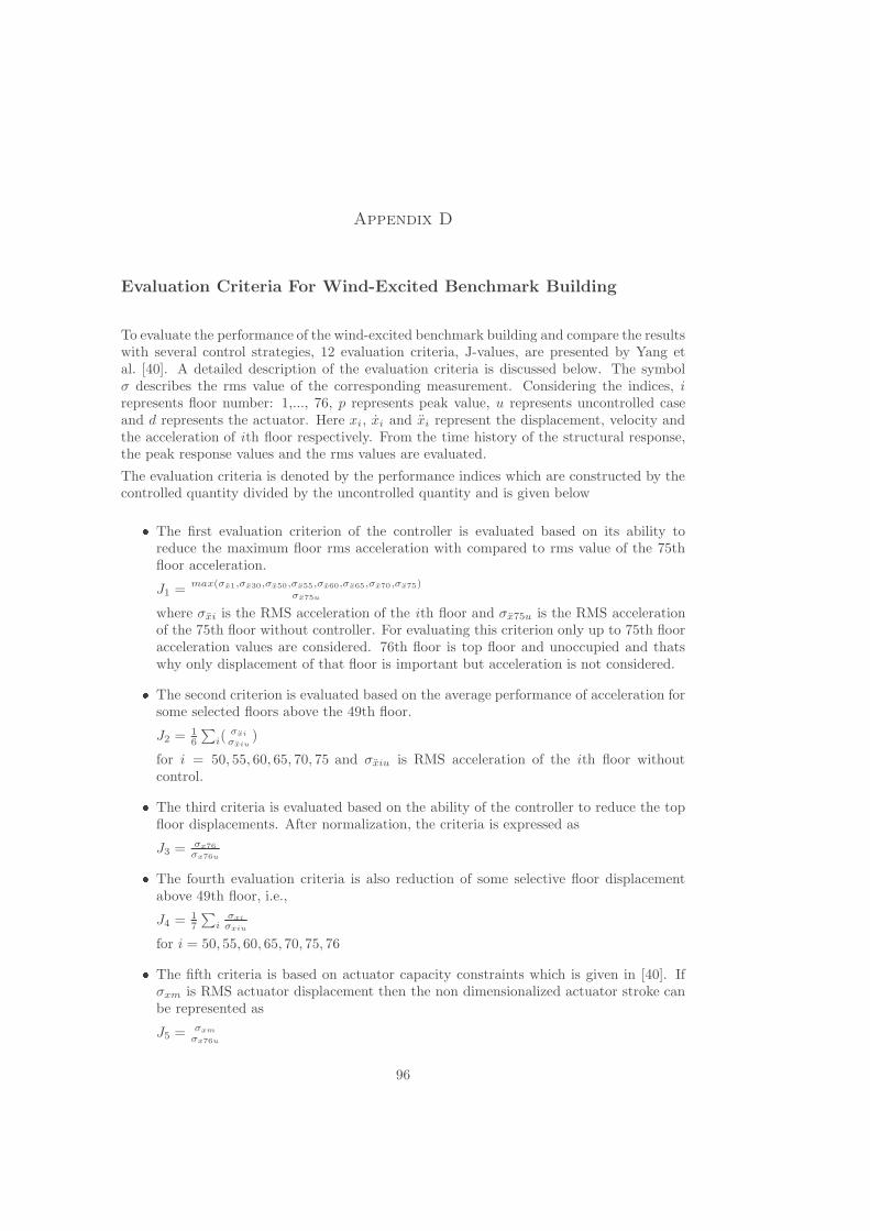
Appendix D
Evaluation Criteria For Wind-Excited Benchmark Building
To evaluate the performance of the wind-excited benchmark building and compare the resultswith several control strategies, 12 evaluation criteria, J-values, are presented by Yang etal. [40]. A detailed description of the evaluation criteria is discussed below. The symbolσ describes the rms value of the corresponding measurement. Considering the indices, irepresents floor number: 1,..., 76, p represents peak value, u represents uncontrolled caseand d represents the actuator. Here xi, xi and xi represent the displacement, velocity andthe acceleration of ith floor respectively. From the time history of the structural response,the peak response values and the rms values are evaluated.
The evaluation criteria is denoted by the performance indices which are constructed by thecontrolled quantity divided by the uncontrolled quantity and is given below
� The first evaluation criterion of the controller is evaluated based on its ability toreduce the maximum floor rms acceleration with compared to rms value of the 75thfloor acceleration.
J1 = max(σx1,σx30,σx50,σx55,σx60,σx65,σx70,σx75)σx75u
where σxi is the RMS acceleration of the ith floor and σx75u is the RMS accelerationof the 75th floor without controller. For evaluating this criterion only up to 75th flooracceleration values are considered. 76th floor is top floor and unoccupied and thatswhy only displacement of that floor is important but acceleration is not considered.
� The second criterion is evaluated based on the average performance of acceleration forsome selected floors above the 49th floor.
J2 = 16
∑i(
σxi
σxiu)
for i = 50, 55, 60, 65, 70, 75 and σxiu is RMS acceleration of the ith floor withoutcontrol.
� The third criteria is evaluated based on the ability of the controller to reduce the topfloor displacements. After normalization, the criteria is expressed as
J3 = σx76
σx76u
� The fourth evaluation criteria is also reduction of some selective floor displacementabove 49th floor, i.e.,
J4 = 17
∑i
σxi
σxiu
for i = 50, 55, 60, 65, 70, 75, 76
� The fifth criteria is based on actuator capacity constraints which is given in [40]. Ifσxm is RMS actuator displacement then the non dimensionalized actuator stroke canbe represented as
J5 = σxm
σx76u
96

97
� The sixth criteria is based on the average power from actuator and represented as
J6 = { 1T
∫ T
0[xm(t)u(t)]2dt}1/2
in which xm is actuator velocity and T is the total time of integration.
� The seventh criteria is based on peak response quantity. The non-dimensional perfor-mance criteria is given as
J7 =max(xp1,xp30,xp50,xp55,xp60,xp65,xp70,xp75)
xp75
� The eighth criterion is the average peak value of acceleration for selected floors above49th floor, i.e.,
J8 = 16
∑i(
xpi
xpiu)
for i = 50, 55, 60, 65, 70 and 75.
where xpi and xpiu are the peak accelerations of the ith floor with and without con-troller.
� The ninth criteria is evaluated based on the ability of the controller to reduce the peakvalue of the top floor displacement. After normalization, the criteria is expressed as
J9 =xp76
xp76u
� The tenth criterion is the average peak value of displacement for selected floors above49th floor, i.e.,
J10 = 17
∑i(
xpi
xpiu)
for i = 50, 55, 60, 65, 70, 75 and 76.
where xpi and xpiu are the peak displacement of the ith floor with and without con-troller.
� The eleventh and twelfth criterions are based on constrains of the actuator capacityin terms of actuator strokes and actuator power respectively
J11 =xpm
xp76u;
J12 = Pmax = max|xm(t)u(t)|
where xpm is peak stroke of actuator and Pmax is the peak control power.

Appendix E
LQG Control Design: Sample Controller In Benchmark Problems
Linear Quadratic Gaussian(LQG) Control is one of the most useful optimal control tech-niques. LQG is used in base-isolated as well as wind-excited benchmark problems as asample controller [39, 40]. The detailed description about formation of LQG controller isdepicted by Yang et al. [40] and also given as below. The LQG controller is used as a sam-ple controller for comparing with the proposed control design methodologies in benchmarkproblems. A brief discussion on LQG control design based on articles [14, 40, 111] is givenbelow
The system model for LQG controller can be full-order or reduced-order based on benchmarkproblem. The reduced-order system model is derived from the full-order system model. Thestandard LQG controller used in benchmark problem is shown in Figure E.1.
Structure
xW
z
+
+
vyKalman
Filter-K
xu
u
Figure E.1: LQG Controller.
The system model is written as
x = Ax+Bu+EW (E.1)
The controlled output equation and the output measurement equation are expressed as
z = Czx+Dzu+ FzW (E.2)
y = Cyx+Dyu+ FyW+ v (E.3)
where x is a n-dimensional state vector consists of displacements and velocities at differentfloor location, z is controlled output vector, y is the measured output vector. A,B,E aresystemmatrices. Cz ,Dz,Fz,Cy,Dy,Fy are output matrices having appropriate dimensions.W is the external excitation and v is the measurement noise which are constructed byuncorrelated Gaussian white noise vectors.
A LQG controller is constructed by minimising a cost function that weights the regulatedoutputs and the control forces is given as
J = limτ→∞
1
τE
[∫ τ
0
(zTaQza + uTRu)dt
](E.4)
98

99
where za = z − FzW = Czx + Dzu, Q is a diagonal matrix that weights the regulatedoutputs andR is an identity matrix that weights the control forces. For the linear system,theseparation principle for LQG method allows the control and estimation problems to beconsidered separately. The control law for the LQG is obtained as
u = −Kx (E.5)
K is obtained fromK = −R
−1(BTP+ ST ) (E.6)
in which P is the solution of the Riccati equation
PA+ ATP−PBR
−1BTP+ Q− SR
−1ST= 0 (E.7)
where Q = CTz QCz, R = DT
zQDz +R, S = CTz QDz and A = A−BR
−1ST . Calculation
of K is performed using MATLAB control toolbox functions lqry .
The LQG controller in (E.5) is based on the state feedback x, which can be estimated fromKalman-Bucy Filter which acts as an observer. The estimated state is denoted by x. TheKalman filter is expressed as
˙x = Ax+Bu+ L(y−Cyx−Dyu) (E.8)
in which the Kalman gain matrix L is calculated from
L = (PkCyT + Sk)Rk
−1 (E.9)
where Pk is obtained from the solution of the Riccati equation
PkA+ ATPk −PkCy
TR−1k CyPk +Qk − SkR
−1k Sk = 0 (E.10)
whereA = AT −CT
y R−1k ST
k (E.11)
Qk and Rk are autopower spectral density function of two vectors EW and FyW + v,respectively. Sk is the cross-power spectral density function of two vectorsEW andFyW+v.
Qk = ESwET ; Sk = ESwF
Ty ; Rk = Sv + FySwF
Ty (E.12)
where Sw and Sv are power spectral density matrices of the white noiseW and v respectively.The Kalman estimator gain L is calculated using MATLAB control toolbox function lqew.


P1
(Journal paper)
Experimental calibration of forward and inverse neural networks for rotary typemagnetorheological damper
Submitted2011


Experimental calibration of forward and inverse neural
networks for rotary type magnetorheological damper
S. Bhowmik a 1, 2, F. Weber * 2 and J. Høgsberg b 1
1Department of Mechanical Engineering, Technical University of Denmark, Lyngby 2800, Denmark
2Empa, Swiss Federal Laboratories for Materials Science and Technology, Structural Engineering Research Laboratory,
Ueberlandstrasse 129, CH-8600 Duebendorf, Switzerland
Abstract. This paper presents a systematic design and training procedure for the feed-forward back-
propagation neural network (NN) modelling of both forward and inverse behaviour of a rotary
magnetorheological (MR) damper based on experimental data. For the forward damper model, with damper
force as output, an optimization procedure demonstrates accurate training of the NN architecture with only
current and velocity as input states. For the inverse damper model, with current as output, the absolute value
of velocity and force are used as input states to avoid negative current spikes when tracking a desired damper
force. The forward and inverse damper models are trained and validated experimentally, combining a limited
number of harmonic displacement records, and constant and half-sinusoidal current records. In general the
validation shows accurate results for both forward and inverse damper models, where the observed
modelling errors for the inverse model can be related to knocking effects in the measured force due to the
bearing plays between hydraulic piston and MR damper rod. Finally, the validated models are used to
emulate pure viscous damping. Comparison of numerical and experimental results demonstrates good
agreement in the post-yield region of the MR damper, while the main error of the inverse NN occurs in the
pre-yield region where the inverse NN overestimates the current to track the desired viscous force.
Keywords: experimental validation, inverse MR damper model, rotary MR damper, neural network.
* Corresponding author, Dr. Mech. Eng., E-mail: [email protected] a Ph.D. student E-mail: [email protected] b Professor, Ph.D. E-mail: [email protected]

1. Introduction
Magnetorheological (MR) dampers used for controlled damping of structural vibrations have received
considerable attention during the last decades because they offer the possibility to adapt their semi-active
force in real-time to the structural vibrations (Christenson et al 2006, Li et al 2007, Neelakantan and
Washington 2008, Wu and Cai 2010). MR dampers are suitable for mitigation of vibrations in large civil
engineering structures because they combine large control force ranges, low power requirements, fast
response time and fail safe performance (Spencer and Nagarajaiah 2003).
Basically, rotary type magnetorheological (MR) dampers consist of a housing including the MR fluid and
the rotating part of the disc. The MR fluid is a suspension of oil with magnetizable particles with average
diameter of 5 �m and some additives. The particles and the ferromagnetic parts of the housing and disc are
magnetized by the magnetic field that is produced by two coils which are installed within the housing on
both sides of the disc. The magnetized particles built chains and thereby stick to the disc and housing (Weber
and Boston 2011a). When the disc starts to rotate the particle chains are initially stretched before they start to
slide relative to the surfaces of the disc and/or the housing. The particle chains may also brake, whereby
rupture between particles occurs. The phase where particle chains are elastically stretched is commonly
denoted as the pre-yield region of the MR fluid, while the sliding phase is called the post-yield region. The
particle chains start to slide when the dry friction force between particles or between particle chains and disc
or between particle chains and housing is balanced by the elastic force due to elongation of the particle
chains (Weber and Boston 2011a). Since this sticking depends strongly on the magnetization of the MR
fluid, and thereby on the MR damper current, the post-yield force of the MR damper typically exhibits a
strong current dependency. Because the superposed viscous force is usually rather small and the MR fluid
viscosity depends only slightly on the coil current, the applied current primarily controls the friction force of
the MR damper, while the viscous force component is mainly governed by the rotating speed of the disc and
the inherent viscosity of the MR fluid (Weber et al 2011). In order to be able to control the total MR damper
force relative to a desired control force, the coil current must be modulated so that the control force tracking
error is acceptable. Due to the non-linear behavior of the MR damper force, i.e. the non-linear relation
between current and sticking force and the non-linear dependency of the MR fluid viscosity on current, force

tracking with force feedback only may fail to track the desired force accurately. Therefore, model-based feed
forward control schemes are needed to solve the force tracking task with sufficient accuracy (Weber et al
2011, Weber and Boston 2011b). Such approaches can then later be extended by a force feedback in order to
further decrease the remaining force tracking error.
MR dampers are either operated at zero or constant current, which are called passive-off or passive-on
strategies (Weber et al 2005), or they are controlled in real-time within a particular feedback loop (Maslanka
et al 2007, Weber et al 2009). In the latter case the structural response is typically measured at damper
position and the MR damper current is controlled in real-time to obtain minimum tracking error with respect
to a desired control force. The force tracking task is usually solved by a model-based feed forward control
scheme, simply to avoid costly force sensors (Maslanka et al 2007, Weber et al 2009). The input states of the
feed forward controller may be the damper displacement, velocity, acceleration, or any combination of these
states, and the desired control force, while the output state is the desired MR damper current. In practice the
desired current is realized by a current driver, which compensates for the coil impedance dynamics of the
MR damper. Therefore, an inverse MR damper model is required that estimates the desired damper current
based on a limited number of the above mentioned input states. This model is usually referred to as an
inverse MR damper model (Tse and Chang 2004, Yang et al 2004, Dominguez et al 2006, Weber et al 2011,
Weber and Boston 2011a, Weber and Boston 2011b) because it predicts the controllable damper current,
while the classic forward models predict the damper force.
Many parametric and non-parametric forward models for classic cylindrical type MR dampers have been
presented in the literature. Some of the prominent parametric approaches are the Bouc-Wen model, which
captures both the pre- and post-yield regions (Yang et al 2004, Dominguez et al 2006), the Bingham model
which basically represents current dependent friction (Ikhouane and Dyke 2007), the Dahl model which
describes an elasto-plastic material behaviour with supplemental viscous effects (Shulman et al 2006) and
the LuGre approach that models the MR fluid particle chains as brushes with sticking and sliding against the
damper housing (Jiménez and Alvarez-Icaza 2005, Yang et al 2009, Boston et al 2010). These models have
also been extended by additional stiffness, viscous and mass elements to account for the accumulator
behaviour, the current dependent viscous force and the inertia of the damper piston and other accelerated

parts (Sahin et al 2010). The parameters for minimum model error are typically obtained from the test data
directly (Sims et al 2004, Weber et al 2008) or by a numerical optimization tool (Ye and Wang 2007). Once
calibrated, these parametric approaches can be used as observers to solve the force tracking problem without
feedback from a force sensor (Maslanka et al 2007, Weber et al 2011, Weber and Boston 2011).
Non-parametric models are mainly based on fitted polynomials (Weber et al 2009), genetic algorithms
(Xiaomin et al 2009), fuzzy logic (Tsoukalas and Uhrig 1997, Won and Sunwoo 2003), neural networks
(NN) (Chang and Roschke 1998, Xia 2003, Chang and Zhou 2002, Wang and Liao 2005, Lee et al 2008,
Metered et al 2009) or hybrid approaches (Soeiro et al 2008). As demonstrated in Chang and Roschke (1998)
the NN approach is able to model the forward MR damper behaviour fairly accurate. Most of the NNs are
trained with simulated input-output data, usually generated by the Bouc-Wen model, as e.g. in Wang and
Liao (2005). Only few NN have been trained with experimental data (Metered et al 2009), containing system
noise and knocking effects due to bearing tolerances. This makes the training of the network much more
difficult, and appropriate filtering of the training data during post processing can be very crucial for the NN
performance. The NN architecture is usually found by a trial and error method, and the resulting NN
architecture is therefore not necessarily optimal with respect to the minimization of the modelling error.
The present investigation provides a systematic approach to the design and calibration of NNs for both
the forward and inverse behaviour of a rotary type MR damper based on experimentally measured training
data. It is shown that only force, velocity and current, with necessary previous states, are sufficient for the
construction of effective NN architectures. For the NN based inverse modelling of the MR damper the
absolute value of velocity and damper force are used as input training data. This modification by the absolute
value in the training data input has a major influence on the proper estimation of the current because the
current is always positive, irrespective of the sign of the training inputs. Moreover, the MR damper
behaviour is measured at constant and half-sinusoidal current, where the half-sinusoidal current tests are
performed because they generate training data very similar to the current records associated with damping of
structures excited at resonance. The experimental data is filtered so that potential noise is minimised and any
offset values are removed. The paper describes a semi-systematic approach for the calibration of the NN
architecture based on the minimization of the associated modelling error. The architecture of the NNs for

both the forward and the inverse MR damper models are presented and validated with measurement data
independent of the training data. Good accuracy is generally reported, and the validated inverse and forward
models are subsequently used in numerical simulations, where pure viscous damping is reproduced real-time.
Figure 1. Experimental set-up with rotary MR damper in hydraulic test machine.
Figure 2. Schematic of test set-up.

2. Experimental data
Section 2.1 introduces the experimental test set-up used to obtain the MR damper response data used for
training of the NN, while the necessary post-processing of the measured time histories is described in
section 2.2.
2.1. Experimental set-up
The MR damper under consideration is a rotary type MR damper with a maximum current of 4 A. The
damper is shown in Fig. 1 and further details on the damper characteristics can be found in Weber et al
(2008) and Boston et al (2010). At constant current the damper behaves almost as a friction damper, with
only a small velocity dependency. The apparent friction force level is approximately 30 N at 0 A and 300 N
at 4 A. Details concerning the behaviour of the rotary type MR damper have been explained in the previous
section. The training and the validation data are obtained from forced displacement tests using a hydraulic
testing machine of type INSTRON, see Fig. 1. The desired piston displacement is defined in Matlab®,
processed real time by a dSPACE® DS1104 R&D controller board and finally send as a command signal
directly to the INSTRON PC unit. A flow diagram of the experimental setup is shown in Fig. 2. The actual
displacement is captured directly as output from the INSTRON machine and acquired by the dSPACE®
system at 1000 Hz sampling frequency. The desired MR damper current is also defined in
Matlab/dSPACE®, and tracked real time by a KEPCO current driver. The actual damper current is measured
by the KEPCO amplifier and acquired by the dSPACE® system. The MR damper force is measured by a
500 N load cell, and the acceleration of the piston is also measured for verification and potential later use in
connection with training or validation. Furthermore, acceleration is suitable for detection of the knocking
effects due to the finite bearing tolerances of 0.01-0.02 mm of the joints of the damper rod. A summary of
the tests conducted is provided in Table 1. Each test is performed twice: The first set is used as training data,
while the second completely independent set is used to validate the NN models. Tests 1-10 are performed at
constant current, while tests 11-19 are conducted with half-sinusoidal current. As seen in Table 1 the desired
displacement is pure sinusoidal, combining amplitudes of 5 mm and 10 mm, and frequencies from 0.5 Hz to
2.2 Hz.

Table 1. Measurement data for training of NN and model validation.
set for trai-ning
set for vali-dation
desired displacement desired current
1a 1b sin, 5 mm, [0.5, 1.0, 1.27, 1.8, 2.2] Hz 0 A
2a 2b sin, 5 mm, [0.5, 1.0, 1.27, 1.8, 2.2] Hz 1 A
3a 3b sin, 5 mm, [0.5, 1.0, 1.27, 1.8, 2.2] Hz 2 A
4a 4b sin, 5 mm, [0.5, 1.0, 1.27, 1.8, 2.2] Hz 3 A
5a 5b sin, 5 mm, [0.5, 1.0, 1.27, 1.8, 2.2] Hz 4 A
6a 6b sin, 10 mm, [0.5, 1.0, 1.27, 1.8, 2.2] Hz 0 A
7a 7b sin, 10 mm, [0.5, 1.0, 1.27, 1.8, 2.2] Hz 1 A
8a 8b sin, 10 mm, [0.5, 1.0, 1.27, 1.8, 2.2] Hz 2 A
9a 9b sin, 10 mm, [0.5, 1.0, 1.27, 1.8, 2.2] Hz 3 A
10ae 10b sin, 10 mm, [0.5, 1.0, 1.27, 1.8, 2.2] Hz 4 A
11a 11b sin, 5 mm, [0.5, 1.0, 1.27, 1.8, 2.2] Hz half-sin, 0 A, [0.5, 1.0, 1.27, 1.8, 2.2] Hz
12a 12b sin, 5 mm, [0.5, 1.0, 1.27, 1.8, 2.2] Hz half-sin, 1 A, [0.5, 1.0, 1.27, 1.8, 2.2] Hz
13a 13b sin, 5 mm, [0.5, 1.0, 1.27, 1.8, 2.2] Hz half-sin, 2 A, [0.5, 1.0, 1.27, 1.8, 2.2] Hz
14a 14b sin, 5 mm, [0.5, 1.0, 1.27, 1.8, 2.2] Hz half-sin, 3 A, [0.5, 1.0, 1.27, 1.8, 2.2] Hz
15a 15b sin, 5 mm, [0.5, 1.0, 1.27, 1.8, 2.2] Hz half-sin, 4 A, [0.5, 1.0, 1.27, 1.8, 2.2] Hz
16a 16b sin, 10 mm, [0.5, 1.0, 1.27, 1.8, 2.2] Hz half-sin, 1 A, [0.5, 1.0, 1.27, 1.8, 2.2] Hz
17a 17b sin, 10 mm, [0.5, 1.0, 1.27, 1.8, 2.2] Hz half-sin, 2 A, [0.5, 1.0, 1.27, 1.8, 2.2] Hz
18a 18b sin, 10 mm, [0.5, 1.0, 1.27, 1.8, 2.2] Hz half-sin, 3 A, [0.5, 1.0, 1.27, 1.8, 2.2] Hz
19a 19b sin, 10 mm, [0.5, 1.0, 1.27, 1.8, 2.2] Hz half-sin, 4 A, [0.5, 1.0, 1.27, 1.8, 2.2] Hz
2.2. Post processing of experimental data
Initially, the measurement data is post-processed by a low pass filter in order to avoid that the NN is trained
by high frequency signal components, e.g. noise and knocking effects, which are typically of no interest. The
applied low pass filter has the following properties:
• Digital Butterworth low pass filter.
• Filter order 2.
• Cut-off frequency 100 Hz.
Any offset in the displacement, acceleration and force signals are removed by simply balancing positive and
negative maxima during steady state conditions. The effect of the filtering of displacement, acceleration,

damper current and damper force is shown in Fig. 3. As seen in Figs. 3(a,c) the high-frequency dithers in the
displacement and damper current are effectively removed by the filter, and the main task is basically to avoid
a too significant change in the phase and reduction in the peak values. The acceleration is very sensitive to
the various sources of noise, and the influence of the filter therefore becomes very evident in Fig. 3(b).
Fig. 3(d) shows the damper force, where the main modification is the removal of the offset level. Note that
the constant force level at zero crossing is due to the previously mentioned bearing tolerance. The effect is
mainly visible in the acceleration signal, which is also shown in Fig. 3(d).
53.4 53.42 53.44 53.46 53.48 53.5−6
−4
−2
0
2
4
6
acce
lera
tio
n [m
/s2]
disp.: sin, 5mm, 1.27Hz; current: 4A
time [s]
filtered &
offset removed
83.2 83.22 83.24 83.26 83.28 83.39.8
10
10.2
dis
pla
ce
me
nt [m
m]
disp.: sin, 10mm, 1.0Hz; current: 4A
10.1
9.9
filtered &
offset
removed
(a) (b)
time [s]
18.44 18.48 18.52 18.56 18.62.92
2.94
2.96
2.98
3
cu
rre
nt [A
]
disp.: sin, 5mm, 0.5Hz; current: half-sin, 3A, 0.5Hz
(c) (d)
filtered
3.02
time [s]55.1 55.2 55.3 55.4 55.5 55.6 55.7
−80
−60
−40
−20
0
20
40
60
80
forc
e [N
]
disp.: sin, 5mm, 2.2Hz; current: half-sin 3A, 2.2Hz
unfiltered
filtered & offset removed
filtered & offset removedacceleration*100 [m/s2]
time [s]
knocking due to
bearing tolerance
visible in acceleration
unfiltered
unfiltered
unfiltered
Figure 3. Filtering of measurement data.
0 100 200 300 400 500 600 700 800 900
0
2
4
6
8
10
12
co
nst.
co
nst.
co
nst.
co
nst.
co
nst.
ha
lf-s
in
ha
lf-s
in
ha
lf-s
in
ha
lf-s
in
ha
lf-s
in
[0.5,1.0,1.27,1.8,2.2] Hz
amplitude of desireddisplacement [mm]amplitude of desiredcurrent [A]
time [s]32.4 32.6 32.8 33 33.2 33.4 33.6
-0.04
-0.03
-0.02
-0.01
0
0.01
0.02
0.03
0.04
estim
ate
d v
elo
city [m
/s]
disp.: sin, 5mm, 1.0Hz; current: 4A
unfiltered
placement*5 [m]
2*pi*1Hz*0.005mm = 0.0314m/s
low pass filtered
filtered & offset
time [s]
(a) (b)
removed dis-
at 20Hz
Figure 4. Estimated velocity (a) and training data time history (b).

The training of the NN also requires the damper velocity x� , which is not directly measured. It is instead
estimated at each time instant k by numerical differentiation of the displacement x as
���
����
�−−
−−=
)1()(
)1()()(
ktkt
kxkxkx� with initial condition 0)1( =x� . (1)
The inherent noise resulting from the numerical differentiation is subsequently removed by the following
low pass filter:
• Digital Butterworth low pass filter.
• Filter order 2.
• Cut-off frequency 20 Hz.
Fig. 4(a) shows the velocity record obtained by differentiation of the sinusoidal displacement with
amplitude 5 mm and frequency 1 Hz. The amplitude of the velocity is 31 mm/s, which agrees well with the
analytical value of mm/s4.31)mm5()Hz1(2 =π . The figure also shows the corresponding displacement,
and it is observed that the phase shift between displacement and velocity is the expected one quarter of a
period. Fig. 4(a) therefore indicates that the method in Eq. (1) leads to a velocity signal with correct
amplitude and phase compared to the associated displacement. After the signal post processing, 10 steady
state cycles of the data sets 1-19 in Table 1 are isolated and then connected after each other to get individual
continuous time histories for displacement, velocity, acceleration, current and force, respectively. Fig. 4(b)
shows the combination system for the generation of the resulting time histories used for training of the NN. It
should be noted that the sets are always connected at zero crossings of the displacement. To have a
reasonably limited amount of data for the training of the NN the time histories are finally down sampled
from 1000 Hz to 200 Hz.
3. Modelling
This section concerns the modelling of the NN, with section 3.1 describing the optimization of the NN
architecture and sections 3.2 and 3.3 presenting the NN models used to model both the forward and the
inverse MR damper characteristics.

x(k)
x(k)
i(k)
x(k)... n
o. d
ela
ys
selections
f(k)
f(k)+-
training
finished?
YES
store
all
dataN
eu
ral N
etw
ork:
i) n
o. h
idd
en
la
ye
rs
ii) n
o. n
eu
ron
s/la
ye
r
transfe
rfunction:
- ta
nsig
fo
r a
ll la
ye
rs
- p
ure
lin fo
r o
utp
ut la
ye
r
change
selections
e(k)
Figure 5. Procedure to find suboptimal NN architecture.
3.1. NN architecture
The modelling of a given system using the NN tool requires basically three steps: (a) measurement of the
input and output states of the system under consideration, (b) choosing the architecture of the particular NN
and (c) training the chosen architecture with the measurement data. The NN architecture is characterized by:
• What states are used as input.
• How many previous values of the input states are used.
• The number of hidden layers and neurons per layer.
• The transfer function of each layer.
Because of the large variety of modelling parameters, the trial and error method is often applied to find an
NN architecture with acceptable modelling errors. Using the trial and error approach the training yields the
best parameters for the chosen NN architecture, but not necessarily the best NN architecture with the best
parameters. In the present work, a semi-systematic approach is used to obtain a near optimal NN
architecture. The procedure is illustrated schematically in Fig. 5. A number of NN are trained to model the
forward MR damper behaviour with the current records and one, or several, of the time histories for
displacement, velocity and acceleration as input states. The number of previous states, the number of hidden
layers and neurons are also varied. For all hidden layers the tangent sigmoid function is chosen as transfer
function, while the linear transfer function is chosen for the output layer. All trained NN candidates are
determined by the Levenberg-Marquardt optimization method, using the )(kerror between the target force

)(kf and the estimated force )(ˆ kf by back propagation. When the training is finished, the individual NN
architecture is stored and a new NN architecture is trained for different input properties. After all possible
combinations of input data have been used for training of the NN architecture, the particular NN architecture
with the smallest modelling error is identified as the best NN architecture, and stored for subsequent
analyses. This systematic optimization strategy shows the following trends:
1. Velocity and damper current are mandatory input states. This is also confirmed by the large number of
parametric MR damper models that are based on velocity and current as input states (Dominguez et al
2004, Maslanka et al 2007, Aguirre et al 2010, Weber et al 2011, Weber and Boston 2011b).
2. Using acceleration as additional input seems to increase the noise in the estimated force without
improving the model accuracy.
3. Using displacement as additional input does not decrease the modelling error. This can be explained
by the fact that the velocity is determined from displacement by Eq. (1) and because the rotary MR
damper has no accumulator and therefore no significant stiffness component.
4. Using both displacement and acceleration as additional input has no influence on the modelling error.
5. It seems that including three previous values, two hidden layers and six neurons per hidden layer
provides a suitable compromise between modelling error and computational effort.
estimated,
low pass
filtered velocity
x(k)
delay
delay
delay
.
x(k-1).
x(k-2).
x(k-3).
i(k)
delay
delay
delay
i(k-1)
i(k-2)
i(k-3)
post processed
current
post processed
force(k)
+_
Ne
ura
l N
etw
ork
fo
rw
ard
dy
na
mic
s:
laye
r 1
, 6
ne
uro
ns, ta
nsig
laye
r 2
, 6
ne
uro
ns, ta
nsig
ou
tpu
t la
ye
r, 1
ne
uro
n, p
ure
lin
err
or(
k)
(a)
f(k)
f(k)
velocity(k)
velocity(k-1)
velocity(k-2)
velocity(k-3) estimated
force(k)
input
Ol O
lO
l
Ol
(1) (2)
(3)
(b)
delay
(0)
g1
g2
g3
delay
delay
input
delay
delay
delay
current(k)
current(k-1)
current(k-2)
current(k-3)
Figure 6. NN architecture of forward MR damper model and its training.
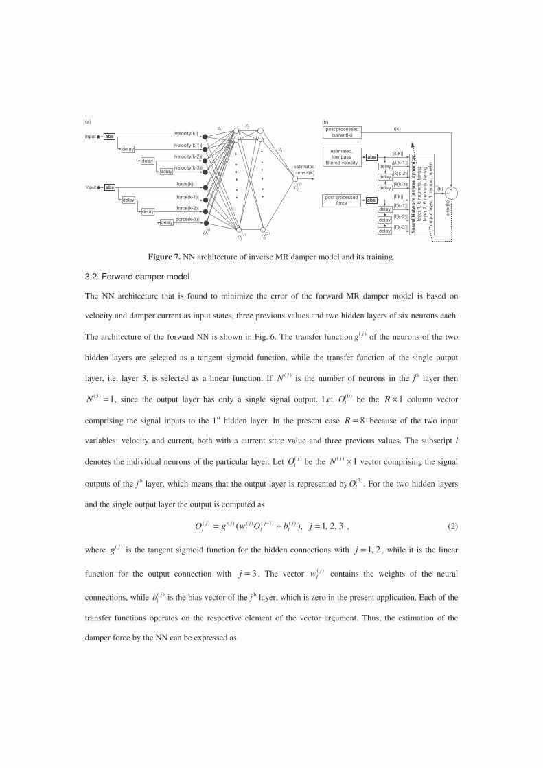
estimated,
low pass
filtered velocity
|x(k)|
delay
delay
delay
.
|x(k-1)|.
|x(k-2)|.
|x(k-3)|.
|f(k)|
delay
delay
delay
|f(k-1)|
|f(k-2)|
|f(k-3)|
post processed
force
post processed
current(k)
+_
err
or(
k)
abs
abs
(a)
i(k)
i(k)
Neu
ral N
etw
ork in
verse d
yn
am
ics:
laye
r 1
, 6
ne
uro
ns, ta
nsig
laye
r 2
, 6
ne
uro
ns, ta
nsig
ou
tpu
t la
ye
r, 1
ne
uro
n, p
ure
lin
|force(k-1)|
|force(k-2)|
|force(k-3)|
|force(k)|
(b)
|velocity(k)|
|velocity(k-1)|
|velocity(k-2)|
|velocity(k-3)| estimated
current(k)
input
Ol O
lO
l
Ol
(1) (2)
(3)
delay
(0)
g1
g2
g3
delay
delay
input
delay
delay
delay
abs
abs
Figure 7. NN architecture of inverse MR damper model and its training.
3.2. Forward damper model
The NN architecture that is found to minimize the error of the forward MR damper model is based on
velocity and damper current as input states, three previous values and two hidden layers of six neurons each.
The architecture of the forward NN is shown in Fig. 6. The transfer function g( j ) of the neurons of the two
hidden layers are selected as a tangent sigmoid function, while the transfer function of the single output
layer, i.e. layer 3, is selected as a linear function. If N ( j ) is the number of neurons in the jth layer then
N (3)=1, since the output layer has only a single signal output. Let Ol
(0)
be the R ×1 column vector
comprising the signal inputs to the 1st hidden layer. In the present case 8=R because of the two input
variables: velocity and current, both with a current state value and three previous values. The subscript l
denotes the individual neurons of the particular layer. Let Ol( j )
be the N ( j )×1 vector comprising the signal
outputs of the jth layer, which means that the output layer is represented by Ol(3). For the two hidden layers
and the single output layer the output is computed as
3,2,1),( )()1()()()(=+=
− jbOwgO jl
jl
jl
jjl , (2)
where g( j ) is the tangent sigmoid function for the hidden connections with 2,1=j , while it is the linear
function for the output connection with 3=j . The vector )( jlw contains the weights of the neural
connections, while bl( j ) is the bias vector of the jth layer, which is zero in the present application. Each of the
transfer functions operates on the respective element of the vector argument. Thus, the estimation of the
damper force by the NN can be expressed as

�
��
−−−
−−−
=
)3()2()1()(
)3()2()1()()(ˆ
kikikiki
kxkxkxkxNNkf
���� (3)
where NN[...] represents the computation by the neural network. For feed forward neural network based
forward dynamics modeling, the network output is ˆ f (k) = Ol(3) whereby ˆ f (k) is the predicted force from
the forward MR model at current time state k. The target of the forward neural network model is
Tl = f (k) (4)
where ( )f k is the desired force, or in this case the measured force data, at current time state k. The network
training was performed using the MATLAB® function trainlm. The network has been trained with the input-
output data sets obtained from the experiments summarized in Table 1. For training of small-to-medium size
networks, the Levenberg-Marquardt algorithm (LM) is fairly efficient. The performance index used for the
training of the feed forward neural network is the sum of squares of the difference el between the desired
target Tl and the actual network output )3(lO ,
,)()( 2)3(
11
2l
I
ll
I
ll OTeV −== ��
==
Z (5)
where Z is a vector containing all network weights and bias values to be optimized, while q is the length of
the data set. The LM algorithm updates the parameters based on minimization of the performance index V .
3.3. Inverse damper model
Fig. 7 shows the corresponding NN for the inverse damper model with velocity and damper force as input
states, and desired damper current as the single output. In order to estimate the MR damper current )(ˆ ki , the
NN for the inverse model uses the actual and three previous values of the two input states,
�
��
−−−
−−−
=
)3()2()1()(
)3()2()1()()(ˆ
kfkfkfkf
kxkxkxkxNNki
���� . (6)
For the feed forward neural network based inverse dynamics modeling of the MR damper, the network
output is )3()(ˆ lOki = where ˆ( )i k is the predicted current from the inverse MR model. The target of the
inverse neural model,
( )lT i k= (7)
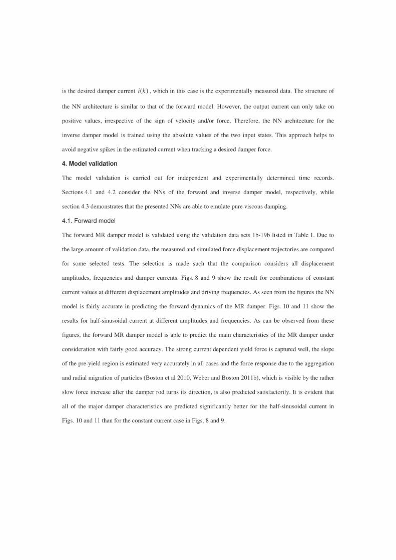
is the desired damper current ( )i k , which in this case is the experimentally measured data. The structure of
the NN architecture is similar to that of the forward model. However, the output current can only take on
positive values, irrespective of the sign of velocity and/or force. Therefore, the NN architecture for the
inverse damper model is trained using the absolute values of the two input states. This approach helps to
avoid negative spikes in the estimated current when tracking a desired damper force.
4. Model validation
The model validation is carried out for independent and experimentally determined time records.
Sections 4.1 and 4.2 consider the NNs of the forward and inverse damper model, respectively, while
section 4.3 demonstrates that the presented NNs are able to emulate pure viscous damping.
4.1. Forward model
The forward MR damper model is validated using the validation data sets 1b-19b listed in Table 1. Due to
the large amount of validation data, the measured and simulated force displacement trajectories are compared
for some selected tests. The selection is made such that the comparison considers all displacement
amplitudes, frequencies and damper currents. Figs. 8 and 9 show the result for combinations of constant
current values at different displacement amplitudes and driving frequencies. As seen from the figures the NN
model is fairly accurate in predicting the forward dynamics of the MR damper. Figs. 10 and 11 show the
results for half-sinusoidal current at different amplitudes and frequencies. As can be observed from these
figures, the forward MR damper model is able to predict the main characteristics of the MR damper under
consideration with fairly good accuracy. The strong current dependent yield force is captured well, the slope
of the pre-yield region is estimated very accurately in all cases and the force response due to the aggregation
and radial migration of particles (Boston et al 2010, Weber and Boston 2011b), which is visible by the rather
slow force increase after the damper rod turns its direction, is also predicted satisfactorily. It is evident that
all of the major damper characteristics are predicted significantly better for the half-sinusoidal current in
Figs. 10 and 11 than for the constant current case in Figs. 8 and 9.

displacement [mm]
forc
e [N
]
disp.: sin, 5mm, 1.0Hz; current: constant, 0A
measured forcepredicted force
(a)
−6 −4 −2 0 2 4 6-80
-60
-40
-20
0
20
40
60
80
displacement [mm]
forc
e [N
]
disp.: sin, 5mm, 0.5Hz; current: constant, 1A
measured forcepredicted force
(b)
−6 −4 −2 0 2 4 6−40
−30
−20
−10
0
10
20
30
40
−6 −4 −2 0 2 4 6−80
−60
−40
−20
0
20
40
60
80disp.: sin, 5mm, 1.27Hz; current: constant, 1A
displacement [mm]
forc
e [N
]
measured forcepredicted force
(c)
−10 −5 0 5 10
-150
-100
-50
0
50
100
150
displacement [mm]
forc
e [N
]
measured forcepredicted force
(d)
disp.: sin, 10mm, 0.5Hz; current: constant, 2A
Figure 8. Validation of forward MR damper model for constant current of 0 A (a), 1 A (b, c) and 2 A (d) and
different displacement amplitudes and frequencies.
−10 −5 0 5 10
−150
−100
−50
0
50
100
150
displacement [mm]
forc
e [N
]
disp.: sin, 10mm, 1.8Hz; current: constant, 2A
measured forcepredicted force
(a)
−6 −4 −2 0 2 4 6-250
-200
-150
-100
-50
0
50
100
150
200
250disp.: sin, 5mm, 1.0Hz; current: constant, 3A
displacement [mm]
forc
e [N
]
measured forcepredicted force
(b)
−6 −4 −2 0 2 4 6
−300
−200
−100
0
100
200
300
displacement [mm]
forc
e [N
]
disp.: sin, 5mm, 1.27Hz; current: constant, 4A
measured forcepredicted force
measured forcepredicted force
(c) (d)
−10 −5 0 5 10
-300
-200
-100
0
100
200
300
displacement [mm]
forc
e [N
]
disp.: sin, 10mm, 2.2Hz; current: constant, 4A
Figure 9. Validation of forward MR damper model for constant current of 2 A (a), 3 A (b) and 4 A (c, d) and
different displacement amplitudes and frequencies.

−6 −4 −2 0 2 4 6−80
−60
−40
−20
0
20
40
60
80disp.: sin, 5mm, 0.5Hz; current: half-sin, 1A, 0.5Hz
displacement [mm]
forc
e [N
]
measured forcepredicted force
−10 −5 0 5 10−80
−60
−40
−20
0
20
40
60
80
displacement [mm]
forc
e [N
]
disp.: sin, 10mm, 1.0Hz; current: half-sin, 1A, 1.0Hz
−10 −5 0 5 10−80
−60
−40
−20
0
20
40
60
80disp.: sin, 10mm, 1.27Hz; current: half-sin, 1A, 1.27Hz
displacement [mm]
forc
e [N
]
measured forcepredicted force
measured forcepredicted force
(a) (b)
(c)
−6 −4 −2 0 2 4 6−80
−60
−40
−20
0
20
40
60
80
displacement [mm]
forc
e [N
]
disp.: sin, 5mm, 1.8Hz; current: half-sin, 1A, 1.8Hz
measured forcepredicted force
(d)
Figure 10. Validation of forward MR damper model for half- sinusoidal current at 1 A and different
displacement amplitudes and frequencies.
−6 −4 −2 0 2 4 6−150
−100
−50
0
50
100
150disp.: sin, 5mm, 1.27Hz; current: half-sin, 2A, 1.27Hz
displacement [mm]
forc
e [N
]
measured forcepredicted force
(a)
−10 −5 0 5 10−150
−100
−50
0
50
100
150disp.: sin, 10mm, 0.5Hz; current: half-sin, 2A, 0.5Hz
displacement [mm]
forc
e [N
]
measured forcepredicted force
−6 −4 −2 0 2 4 6-150
-100
-50
0
50
100
150disp.: sin, 5mm, 2.2Hz; current: half-sin, 2A, 2.2Hz
displacement [mm]
forc
e [N
]
measured forcepredicted force
(b)
−10 −5 0 5 10-150
-100
-50
0
50
100
150disp.: sin, 10mm, 1.8Hz; current: half-sin, 2A, 1.8Hz
displacement [mm]
forc
e [N
]
measured forcepredicted force
(d)(c)
Figure 11. Validation of forward MR damper model for half-sinusoidal current at 2 A and different
displacement amplitudes and frequencies.

4.2. Inverse model
The inverse MR damper model is also validated using the validation data sets 1b-19b in Table 1. The results
for constant current, two different displacement amplitudes and four different displacement frequencies are
shown in Figs. 12(a,b). The estimated current shows significant local spikes that might arise because the NN
architecture has also been trained with half-sinusoidal current data or from the bearing plays of the damper
rod joints at zero-crossing of the velocity. Although the bearing plays are on the order of 0.02 mm or less,
force knocking effects cannot be avoided when the piston of the hydraulic machine turns its direction and
thereby the damper force and velocity undergo zero-crossings. This hypothesis is partly verified by the fact
that the spikes show the same frequency characteristics as the applied displacement. Similar results have also
been reported in Wang and Liao (2005) and Metered et al (2009). This fact might indicate that the NN is
fairly sensitive to high frequency signal inputs and has only little low pass behaviour. In contrast to the
prediction of constant current, the prediction of the half-sinusoidal current is fairly accurate for different
displacement amplitudes, frequencies and current amplitudes as shown in Figs. 12(c,d), 13 and 14. However,
also this model validation test shows current spikes and therefore local modelling errors at each half period.
Since these spikes occur later than the current maximum, which means after the hydraulic piston has turned
its direction, the current spikes cannot result from the force knocking effects at zero velocity crossing, but
may instead result from the Stribeck effect, which occurs at the transition between the pre- and post-yield
regions. Despite the apparent modelling error due to the spikes of the estimated current, these spikes are
rather small compared to e.g. the validation results presented in Wang and Liao (2005).

a a+0.5 a+1 a+1.5 a+2
0
1
3
4
5
a a+0.5 a+1 a+1.5 a+2
0
1
3
4
5
cu
rre
nt [A
]
predicted current for:
predicted current for:
predicted current for:
time [s]time [s]
(a) (b)
25 26 27 28 29
0
1
3
4
time [s]
0.5Hz, 5mm 1.0Hz, 5mm
44.5 45 45.5 46 46.5 47
1.27Hz, 5mm 1.8Hz, 5mm
time [s]
(c) (d)
4A; 5mm, 1.27Hz
2A; 5mm, 2.2Hz
0A; 5mm, 1.8Hz
predicted current for:
predicted current for:3A; 10mm, 0.5Hz
1A; 10mm, 1.0Hzcu
rre
nt [A
]
0
1
3
4
cu
rre
nt [A
]cu
rre
nt [A
]
predicted
measuredcurrent
currentpredicted
measuredcurrent
current
Figure 12. Validation of inverse MR damper model for constant current (a, b) and half-sinusoidal current at
3 A (c, d).
55 55.5 56 56.5 57 57.5
0
1
3
4
time [s]
(a)
2.2Hz,0.5Hz, 10mm5mm
84.5 85 85.5 86 86.5
0
1
3
4
time [s]
1.27Hz, 10mm1.0Hz, 10mm(b)
98.6 98.8 99 99.2 99.4 99.6
0
1
3
4
time [s]
2.2Hz, 10mm1.8Hz, 10mm(c) (d)
25.5 26 26.5 27 27.5 28 28.5 29
0
1
3
4
time [s]
1.0Hz, 5mm0.5Hz, 5mm
cu
rre
nt [A
]
predicted
measuredcurrent
current
cu
rre
nt [A
]cu
rre
nt [A
]
cu
rre
nt [A
]
predicted
measuredcurrent
currentpredicted
measuredcurrent
current
predicted
measuredcurrent
current
Figure 13. Validation of inverse MR damper model for half- sinusoidal current at 3 A (a-c) and 4 A (d).

44.6 44.8 45 45.2 45.4 45.6 45.8 46 46.2 46.4
0
1
3
4
time [s]
1.8Hz, 5mm1.27Hz, 5mm
(a)
55 55.5 56 56.5 57 57.5
0
1
3
4
time [s]
0.5Hz, 10mm2.2Hz, 5mm
(b)
84.5 85 85.5 86 86.5
0
1
3
4
time [s]
1.27Hz, 10mm1.0Hz, 10mm
(c) (d)
98.4 98.6 98.8 99 99.2 99.4
0
1
3
4
time [s]
2.2Hz, 10mm1.8Hz, 10mm
predicted
measuredcurrent
current
predicted
measuredcurrent
current
predicted
measuredcurrent
current
predicted
measuredcurrent
current
cu
rre
nt [A
]cu
rre
nt [A
]
cu
rre
nt [A
]cu
rre
nt [A
]
Figure 14. Validation of inverse MR damper model for half- sinusoidal current at 4 A (a-d).
4.3. Emulation of viscous damping using validated models
In this section the forward and inverse models are used to demonstrate how accurate pure viscous damping
can be emulated by the rotary MR damper of the present study. Fig. 15(a) shows the flow chart of this
simulation. The velocity of the MR damper is assumed to be pure sinusoidal. This is a reasonable assumption
for damping of lightly damped structures, where the structural response is typically dominated by resonance
at the frequency of the critical vibration mode and with a slowly varying amplitude envelope. The desired
control force is the product of velocity and the viscous coefficient c . The damper velocity and the desired
control force are used as the input states for the inverse MR damper model, which then estimates the
corresponding damper current that is applied to the MR damper in order to generate a pure viscous force.
This force is estimated using the forward MR damper model. If the NN for the inverse and the forward MR
damper model are sufficiently accurate the simulated damper force should be comparable to the
corresponding pure viscous damper force. The simulation results are shown in Figs. 15(b-d). The simulated
current in Figs. 15(b) exhibits two significant spikes on top of the approximately half-sinusoidal time history.
The first spike should not occur because the desired force decreases to zero. Hence, zero current

−0.15 −0.1 −0.05 0 0.05 0.1 0.15
-100
-50
0
50
100desired force
simulated force
velocity [m/s]
forc
e [N
]
0.2 0.4 0.6 0.8 1 1.2 1.4−1
−0.5
0
0.5
1
1.5
2
time [s]
disp.: sin, 20mm, 1.27Hz; emulation of viscous damping
velocity*5 [m/s]simulated current [A]
−300
−200
−100
0
100
200
300
desired force
simulated force
0.2 0.4 0.6 0.8 1 1.2 1.4time [s]
inverse model
velocity input (disp.: sin, 20mm, 1.27Hz)
c
desired force
simulated current
forward model
simulated force
viscous coefficient c
(a) (b)
(c) (d)
(data during 0.2-0.987s)
Figure 15. Simulated emulation of viscous damping: Flow chart (a), simulated MR damper current (b) and
simulated MR damper force (c, d).
would be the best choice to track the desired viscous force as precise as possible. The second current spike
occurs when the MR fluid is operated within the pre-yield region. This spike is therefore needed because the
actual MR damper force at 0 A within the pre-yield region is smaller than the desired viscous force that
increases rapidly at displacement extremes due to the elliptic force displacement trajectory of viscous
damping (Maslanka et al 2007). When the MR fluid is operated in the post-yield region, the current shows
approximately a half-sinusoidal behaviour because of the pure sinusoidal behaviour of the desired force, see
Fig. 15(c). The main discrepancies are mainly due to the non-linear relation between yield force and current
and the force response, arising because of the inherent migration and aggregation of the particles in the MR
fluid (Weber et al 2008, Boston et al 2010). Despite the mediocre estimate of the current at zero velocity and
the slightly overestimated current during the pre-yield region, the time history of the damper force in
Fig. 15(c) and the force velocity trajectory in Fig. 15(d) demonstrate that pure viscous damping is in fact
tracked fairly accurate at velocities larger than 0.05 m/s. The obtained results indicate that the NNs have

difficulties to accurately estimating the behaviour of the MR damper in the pre-yield region, which produces
current spikes and thereby significant force tracking errors at small velocities. However, effective structural
damping is mainly governed by the energy dissipation at large velocities, why these low-velocity current
spikes are only of minor importance for most practical applications.
5. Summary and Conclusions
This paper describes the feed forward back propagation neural network based modelling of the forward and
the inverse behaviour of a rotary MR damper using experimentally measured data for both training and
validation. The measured data has been low pass filtered in order to remove high frequency signal parts that
might have significant influence on the performance of the NN. The measured data comprising two
displacement amplitudes, five frequencies and both constant and half-sinusoidal current has been combined
to get a single sequential time history and afterwards down-sampled from 1000 Hz to 200 Hz to optimize the
training of the NN architecture. An optimization procedure has been presented to identify the NN
architecture that minimizes the error of the forward model. For training the procedure has been tested with
combinations of measured displacement, velocity, acceleration and damper current as input states.
Furthermore, the number of previous values of the input states and the number of hidden layers and neurons
have been altered to obtain the best numerical fit. To limit the computational time of this numerical
optimization, the transfer functions for the hidden and output layers were fixed to the tangent sigmoid
function and the linear function, respectively. The present procedure demonstrates that the modelling error is
not decreased significantly:
• if displacement and acceleration are taken as inputs in addition to velocity, and
• if substantially more than three past values of the inputs are taken into account, and
• if substantially more than two hidden layers of more than six neurons are considered.
The same NN architecture has also been used to model the inverse MR damper behaviour. In this case the
damper current is the output, while the absolute values of damper force and velocity are used as input states.
The introduction of the absolute values as the input to the NN minimizes the possibility of negative spikes in
the estimated damper current when e.g. tracking a desired viscous force.

The trained forward and inverse MR damper models have been validated with measurement data that is
independent of the training data at different displacement amplitudes and frequencies. The validation data
comprises test records at two displacement amplitudes, five frequencies and both constant and half-
sinusoidal damper current signals. The validation shows that the forward model is able to predict the MR
damper force with high accuracy. Especially the force response due to the migration and aggregation of the
MR fluid particles is captured well, and the slope of the force displacement trajectory in the pre-yield region
is predicted accurately. The validation of the inverse MR damper model shows two particular characteristics.
When the measurement data has been obtained from constant current, the predicted current records contain
significant spikes with the same frequency as the damper displacement. This might therefore result from
force knocking effects at displacement extremes due to the inherent bearing plays between the damper rod
and the hydraulic machine, which are of the order of 0.02 mm. For these tests, only the mean value of the
predicted current is accurate. In contrast, the prediction based on the half-sinusoidal current turns out to give
more accurate results for all amplitudes and frequencies used in the tests. Nevertheless, also this validation
shows current spikes which do not occur at the time of displacement extremes, but later. This indicates that
these spikes are forced by the Stribeck effect, which occurs between the pre- and post-yield regions.
The validated forward and inverse MR damper models are finally used to simulate the emulation of
viscous damping. The simulation shows that the inverse model overestimates the current in the vicinity of
zero velocity, i.e. in the pre-yield region, while the output current is quite accurate within the post-yield
region. As a result, the force tracking error is fairly large at small damper velocities, but considerably smaller
at velocities where the MR damper is not operated in the pre-yield region.
This investigation shows that the NN technique can be used to model the inverse MR damper behaviour
and thereby effectively solve the force tracking task with sufficiently small force tracking error.
Acknowledgement
The work is supported via the research grant Damping of Flexible Structures by Smart Control of Semi
Active devices by the Danish Council of Research and Innovation. The authors also gratefully acknowledge
the use of the testing facilities as well as the technical assistance of Empa, Swiss Federal Laboratories for

Materials Science and Technology, Dübendorf, Switzerland, and the technical support of the industrial
partner Maurer Söhne GmbH & Co. KG, Munich, Germany.
References
Aguirre, N., Ikhouane, F., Rodellar, J., Wagg. D.J. and Neild, S.A. (2010), “Viscous and Dahl model for
MR dampers characterization: A Real time hybrid test (RTHT) validation”, Proceedings of the 14th
European Conference on Earthquake Engineering, August 30 - September 03, 2010, Ohrid, Republic of
Macedonia.
Boston, C., Weber, F. and Guzzella, L. (2010), “Modeling of a disk-type magnetorheological damper”,
Smart Mater. Struct., 19 045005.
Chang, C. and Roschke, P. (1998), “Neural network modeling of a magnetorheological damper”,
Journal of Intelligent Material Systems and Structures, 9, 755-64.
Chang, C. and Zhou, L. (2002), “Neural network emulation of inverse dynamics for a
magnetorheological damper”, Journal of Structural Engineering, 128, 231-9.
Christenson, R.E., Spencer, Jr.B.F. and Johnson, E.A. (2006), “Experimental verification of smart cable
damping”, Journal of Engineering Mechanics, 132(3), 268-78.
Dominguez, A., Sedaghati, R. and Stiharu, I. (2004), “Modelling the hysteresis phenomenon of
magnetorheological dampers”, Smart Mater. Struct., 13, 1351-61.
Dominguez, A., Sedaghati, R. and Stiharu, I. (2006), “A new dynamic hysteresis model for
magnetorheological dampers”, Smart Mater. Struct., 15, 1179-89.
Ikhouane, F. and Dyke, S. (2007), “Modeling and identification of a shear mode magnetorheological
damper”, Smart Mater. Struct., 16, 605-16.
Jiménez, R. and Alvarez-Icaza, L. (2005), “LuGre friction model for a magnetorheological damper”,
Journal of Structural Control and Health Monitoring, 12, 91-116.
Lee, H., Jung, H., Cho, S. and Lee, I. (2008), “An experimental study of semiactive modal neuro-control
scheme using MR damper for building structure”, Journal of Intelligent material Systems and Structures, 19,
1005-15.

Li, H., Liu, M., Li, J., Guan, X. and Ou, J. (2007), “Vibration control of stay cables of the Shandong
Binzhou yellow river highway bridge using magnetorheological fluid dampers”, Journal of Bridge
Engineering, 12(4), 401-9.
Maslanka, M., Sapinski, B. and Snamina, J. (2007), “Experimental study of vibration control of a cable
with an attached MR damper”, Journal of Theoretical and Applied Mechanics, 45(4), 893-917.
Metered, H., Bonello, P. and Oyadiji, S.O. (2009), “The experimental identification of
magnetorheological dampers and evaluation of their controllers”, Journal of Mechanical Systems and Signal
Processing, 24, 976-94.
Neelakantan, V.A. and Washington, G.N. (2008), “Vibration control of structural systems using MR
dampers and a ‘modified’ sliding mode control technique”, Journal of Intelligent Material Systems and
Structures, 19(2), 211-24.
Sahin, I., Engin, T. and Cesmeci, S. (2010), “Comparison of some existing parametric models for
magnetorheological fluid dampers”, Smart Mater. Struct., 19, 035012 (11pp).
Shulman, Z.P., Korobko, E.V., Levin, M.L. et al. (2006), “Energy dissipation in electrorheological
damping devices”, Journal of Intelligent Material Systems and Structures, 17(4), 315-20.
Sims, N.D., Holmes, N.J. and Stanway, R. (2004), “A unified modelling and model updating procedure
for electrorheological and magnetorheological vibration dampers”, Smart Mater. Struct., 13(1), 100-21.
Soeiro, F.J., Stutz, L.T., Tenenbaum, R.A. and Neto, A.J. (2008), “Stochastic and hybrid methods for
the identification in the Bouc-Wen model for magneto-rheological dampers”, Journal of Physics: conference
series, 135, 012093.
Spencer, Jr.B.F. and Nagarajaiah, S. (2003), “State of the art of structural control”, Journal of Structural
Engineering, 129(8), 845-56.
Tse, T. and Chang, C. (2004), “Shear-mode rotary magnetorheological damper for small-scale structural
control experiments”, Journal of Structural Engineering, 130, 904-10.
Tsoukalas, L. and Uhrig, R. (1997), Fuzzy and Neural Approaches in Engineering, John Wiley & Sons
Inc.

Wang, D.H. and Liao, W.H. (2005), “Modeling and control of magnetorheological fluid dampers using
neural networks”, Smart Mater. Struct., 14, 111-26.
Weber, F., Feltrin, F. and Distl, H. (2008), “Detailed analysis and modeling of MR dampers at zero
current”, Structural Engineering Mechanics, 30, 787-90.
Weber, F. and Boston, C. (2011a), “Measured tracking of negative stiffness with MR damper”,
Proceedings of the 5th ECCOMAS Thematic Conference on Smart Structures and Materials, Saarbrücken /
Germany, on July 6 - 8, 2011, on CD.
Weber, F., Boston, C. and Maslanka, M. (2011), “Adaptive TMD based on the emulation of positive
and negative stiffness with MR damper”, Smart Mater. Struct., 20, 015012 (11pp).
Weber, F. and Boston, C. (2011b), “Clipped viscous damping with negative stiffness for semi-active
cable damping”, Smart Mater. Struct., 20, 045007 (13pp).
Weber, F., Feltrin, G. and Motavalli, M. (2005), “Passive damping of cables with MR dampers”,
Journal of Materials and Structures, 38(279), 568-77.
Weber, F., Distl, H., Feltrin, G. and Motavalli, M. (2009), “Cycle energy control of MR dampers on
cables”, Smart Mater. Struct., 18(1), 015005.
Won, J. and Sunwoo, M. (2003), “Fuzzy modelling approach to magnetorheological dampers: forward
and inverse model”, Journal of Systems and Control Engineering, 20, 1055-65.
Wu, W.J. and Cai, C.S. (2010), “Cable vibration control with a semiactive MR damper - numerical
simulation and experimental verification”, Structural Engineering and Mechanics, 34(5), 611-23.
Xia, P. (2003), “An inverse model of MR damper using optimal neural network and system
identification”, Journal of Sound and Vibration, 266, 1009-23.
Xiaomin, X., Qing, S., Ling, Z. and Bin, Z. (2009), “Parameter estimation and its sensitivity analysis of
the MR damper hysteresis model using a modified genetic algorithm”, Journal of Intelligent Material
Systems and Structures, 20(17), 2089-100.
Yang, G., Spencer, Jr.B.F., Jung, H.-J. and Carlson, J.D. (2004), “Dynamic modeling of large-scale
magneto-rheological damper systems for civil engineering applications”, Journal of Engineering Mechanics,
130(9), 1107-14.

Yang, F., Sedaghati, R. and Esmailzadeh, E. (2009), “Development of LuGre friction model for large-
scale magneto-rheological fluid damper”, Journal of Intelligent Material Systems and Structures, 1 doi:
10.1177/1045389X08099660.
Ye, M. and Wang, X. (2007), “Parameter estimation of the Bouc-Wen hysteresis model using particle
swarm optimization”, Smart Mater. Struct., 16, 2341-49.

P2
(Journal paper)
Design and experimental verification of semi-active control with negative stiffness for MRdampers
Submitted2011


Design and experimental verification of semi-active control
with negative stiffness for MR dampers
F Weber1,#, S Bhowmik
1,2 and J Høgsberg2
(1) Empa, Swiss Federal Laboratories for Materials Science and Technology, Structural Engineering
Research Laboratory, Ueberlandstrasse 129, CH-8600 Duebendorf, Switzerland
E-mail: [email protected]
(2) Department of Mechanical Engineering, Technical University of Denmark, Lyngby 2800, Denmark
E-mail: [email protected], [email protected]
(#) Author to whom any correspondence should be addressed.
Abstract
For external damping of flexible structures the introduction of negative damper stiffness in the damper force
locally increases the deformation of the structure at damper position and thereby the energy dissipation in the
external damper. For a suitable design of the negative stiffness and the damping forces this concept may
improve the damping of the structure. The present paper considers both a linear control model, with a
viscous term and a negative stiffness term, and a non-linear model composed of friction and negative
stiffness. Expressions are derived for the calibration of these control models. However, the introduction of
negative stiffness may produce active parts in the desired damper force, and in semi-active control these
parts are typically clipped. The linear control model requires the clipping independent of the viscous and
negative stiffness terms which may lead to a reduction in the attainable damping and an increase in high
frequency noise in the structure. In contrast, the non-linear model does not need to be clipped if the friction
force level is controlled in proportion to the damper displacement amplitude and balances the maximum
negative stiffness force. The performances of both control strategies are verified by experiments, where a
magnetorheological damper acts on a five storey shear frame structure. The tests show that negative damper
stiffness can enhance the structural damping significantly compared to pure viscous damping. Due to the
clipping, the linear model leads to smaller structural damping than theoretically expected and to additional
high frequency components in the structure. In contrast, the non-linear model, which does not need to be
clipped for proper choice of friction and stiffness, almost generates the theoretically expected structural
damping and the high frequency components introduced by the non-linear friction force by the controlled
magnetorheological damper are limited.
1. Introduction
Magneto-rheological (MR) dampers are commonly used for controlled vibration mitigation of civil
engineering structures because they are fail safe and reliable due to their dissipative nature and residual force
level at 0 A, and because proper semi-active control combines the advantages of active and passive damping,
see e.g. [1]. For damping of stay cables the potential associated with controlled MR dampers has been
investigated by simulation, laboratory and field tests in several research projects. A general overview can be
found in the references [2-10]. Similarly, the vibration reduction of civil engineering structures -- such as
buildings, bridges and models of these structures – by controlled MR dampers has been simulated and/or
tested experimentally in [11-26]. Also, controlled MR dampers have been installed in tuned mass dampers
[27-29] or in tuned masses [30, 31] in order to make these otherwise passive devices adaptive. Many
different clipped active, semi-active and passive control laws have been tested and verified for MR dampers.
Among these the so-called clipped optimal control schemes are presented in e.g. [2-4, 7], the clipped viscous

model with negative stiffness is investigated in e.g. [9], various semi-active algorithms have been proposed
in [32, 33] and simple passive approaches such as controlled viscous damping, controlled friction damping
and controlled energy dissipation have been proposed and analysed in [5], [2, 16, 34] and [8], respectively.
For model-based control of semi-active dampers the real-time tracking of the desired damper force can be
solved in different ways. The Heaviside step function – or on/off – approach requires the measuring of the
actual MR damper force, as described in e.g. [35]. The force tracking can also be based on the inversion of
sufficiently simple mathematical models, as for example the Bingham plasticity model [5, 9, 11].
Alternatively, more detailed and validated models can be used as observers, which has been demonstrated in
[36-38] for the LuGre friction model. A mapping approach based on tests of the MR damper connected to a
cable is presented in [8], neural network based force tracking approaches have been developed in [39-43] and
also fuzzy logic [44] and other methods [45] have been adopted to capture the inverse dynamics of an MR
damper.
In recent years, the structural damping due to the emulation of a negative stiffness force besides the
damping force in the MR damper has been investigated in several research projects [4, 9, 32, 33, 46-49]. As
described in [9], larger structural damping is achieved because the negative stiffness force increases the
motion in the damper, which leads to an increase in energy dissipation per cycle in the damper when
compared to for instance a pure viscous damper [51]. It has also been shown in [4, 9, 49] that clipped optimal
control of a cable with a semi-active damper results in approximately the same control force behaviour as for
simple clipped viscous damping with negative stiffness.
The aim of the present paper is to demonstrate and experimentally verify the influence of negative
stiffness in the semi-active control of an MR damper. The tracking of the desired damper force by the MR
damper is provided by a validated neural network with absolute values of damper velocity and desired
damper force as network input, and the desired MR damper current as the output. Details on the training and
validation of the neural network can be found in [39]. The benchmark damper model is the pure viscous
damper, while the control laws of interest in the present study are the linear model with a viscous term and a
negative stiffness term and the non-linear model with a friction term and a negative stiffness term. The non-
linear approach has been introduced in [32, 33]. Based on a free approximate vibration analysis theoretical
estimates are derived for the damper calibration associated with maximum modal damping ratio of the
targeted vibration form. It is found by the theoretical results that a substantial increase in damping
performance can be expected for the ideal linear control model. However, in a linear model negative stiffness
produces active control forces, which must be clipped or truncated in a semi-active control environment. It is
illustrated by simulations and experiments that this clipped linear model with negative stiffness improves the
damping performance compared to the pure viscous damper. However, it is also indicated that the clipping
yields a significant reduction in the performance compared to the theoretical predictions. On the other hand
the friction force level and the negative stiffness component of the non-linear model are balanced so that in
steady-state harmonic conditions clipping is avoided. Furthermore, the friction force level of the non-linear
control model is adaptively changed according to the collocated response amplitude. This secures effective
damping of the structure. Simulations and in particular experiments show that this non-linear model is not
affected as much by clipping as the linear model, and it more or less provides the performance predicted by
the theory. This shows that, although clipping of linear active control methods lead to improved semi-active
damping compared to passive methods, the formulation of non-linear control strategies, which take the
inherent properties of the MR damper into account, result in robust and effective damping of the flexible
structure.
The outline of the paper is as follows. In Section 2 the general results for free vibrations of the structure
with a local damper are reviewed. The details on this approach are presented in e.g. [50, 51]. These results
are applied in Section 3 to derive the calibration of the various control strategies based on maximization of
the modal damping ratio for the targeted vibration mode. These results show that the non-linear control
results in an attainable damping ratio that is twice the value of pure viscous damping, while the linear control
method with negative stiffness potentially leads to a very significant increase in modal damping. The
performance of the control strategies is investigated in Section 4 by simulations and experiments, where a
rotational MR damper is operating on a shear frame model structure. The experiments show that due to
heavy clipping of the present linear model with negative stiffness the predicted efficiency is significantly
reduced, while the performance of the adaptively controlled non-linear model is more or less maintained.

Section 4 also gives an overview of practical aspects related to the experiments, while the construction and
validation of the numerical model for the shear frame structure is presented in Appendix A.
2. Damping of Structures
The discretized equations of motion for a flexible structure can be written in the classic matrix form
extf� � � � �Mx Cx Kx v f�� � (1)
where x contains the degrees of freedom, M is the mass matrix, C is the structural damping matrix and
K is the stiffness matrix. The external damping is provided by the single damper force f , where the
connectivity vector v represent the point of action of the damper force on the structure. The external loading
is governed by the vector function extf . The minus on the damper force implies that f in the theoretical
derivations is considered as an internal force.
The calibration of the various semi-active control strategies presented in Section 3 is based on the
maximization of the damping ratio of the targeted vibration mode. An explicit estimate of the modal
damping ratio can be determined following the system reduction technique in [50, 51]. The characteristics of
the system are governed by the free vibrations without structural damping. In the frequency domain the
equation of motion (1) can be written as
� �2 f�� � � �M K x v (2)
where x and f are the frequency amplitudes of the response vector and damper force, respectively. In the
frequency domain formulation it is convenient to formulate the damper forces as
( )f H x�� (3)
introducing the frequency dependent damper function ( )H � . The damper format is collocated, which
means that the damper force is proportional to the energetically conjugate damper displacement, given in
terms of the connectivity vector by Tx � v x . The frequency function in (3) is in general complex valued,
( ) Re ( ) Im ( )H H i H� � �� � (4)
where i is the imaginary unit. The real value represents the stiffness component in phase with displacement,
while the imaginary part represents the damping component out-of-phase with displacement and thereby in
phase with velocity.
As demonstrated in [50] the modal response of the structure with the damper acting on the structure can
be effectively represented by the two-component representation,
0 0r r� �� �x u u (5)
where 0u is the vibration form of the target mode without the damper, while �u is the corresponding
vibration form with the damper link fully locked. The frequency amplitudes 0r and r� represent the degrees
of freedom of the two-dimensional subspace. The limiting vibration forms are illustrated in Fig. 1 for a five
storey shear frame structure with the damper acting on the relative motion between the first floor and ground,
see Fig. 1a. For this damper configuration the connectivity vector is T]0,0,0,0,1[�v .

Figure 1. (a) Structure with external damper, (b) vibration form without damper, and (c) vibration form with
damper link fully locked.
The two limiting vibration forms are governed by the eigenvalue problems derived from (2) when
0H � and H � � , respectively. They are conveniently formulated as
� � � �2 2
0 0 ,� �� � �� � � �K M u 0 K M u 0 (6)
where the locked stiffness matrix is given as � �0lim T
g g� ��� �K K vv . In the following the vibration
forms are normalized to unit modal mass, whereby the corresponding natural frequencies are determined
directly from the corresponding modal stiffness as 2
0 0 0
T� � u Ku and 2 T�� � � �� u K u .
As demonstrated in e.g. [51] an approximate solution for the complex valued natural frequency � can be
obtained by projection of the equation of motion (2) on to the reduced subspace governed by the two-
component representation in (5). The damping ratio Im / � �� represents the relative imaginary part
of the complex natural frequency, and an explicit expression for the damping ratio of the target mode can be
written as
� �
00
2 220 0 0
2 Im ( )
1 Re ( ) Im ( )
H
H H
� �� �
� � � � � �
�
�
�
� � �� (7)
where the magnitude of the natural frequency has been approximated by the mean value � �0 / 2� � ���� .
In (7) the damper function H is normalized by the parameter
� �
2
0
2 2
0
T
�� ��
��
v u (8)
The magnitude of the damper function H is in the following calibrated to provide maximum modal damping
to the targeted mode. It follows from (7) that the attainable damping ratio depends on the particular relation
between real and imaginary part of the damper function H . However, it is observed from (7) that a
reduction in the damper stiffness (real part) implies a potential increase in the damping ratio. For linear
control strategies the application of negative stiffness requires active control forces, while for semi-active
control these active parts are simply clipped. In Section 4 it is demonstrated that with an adaptive control
scheme, formulated specifically for an MR type damper, the clipping can be avoided and apparent negative
stiffness will effectively improve the damping performance. The calibration with respect to maximum
damping ratio is presented for the various control strategies in Section 3.
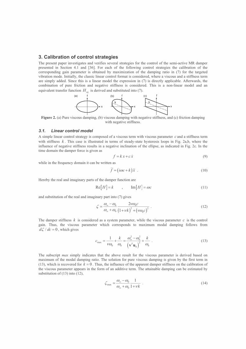
3. Calibration of control strategies
The present paper investigates and verifies several strategies for the control of the semi-active MR damper
presented in Section 4.1 and [36]. For each of the following control strategies the calibration of the
corresponding gain parameter is obtained by maximization of the damping ratio in (7) for the targeted
vibration mode. Initially, the classic linear control format is considered, where a viscous and a stiffness term
are simply added. Since this is a linear model the expression in (7) is directly applicable. Afterwards, the
combination of pure friction and negative stiffness is considered. This is a non-linear model and an
equivalent transfer function eqH is derived and substituted into (7).
Figure 2. (a) Pure viscous damping, (b) viscous damping with negative stiffness, and (c) friction damping
with negative stiffness.
3.1. Linear control model A simple linear control strategy is composed of a viscous term with viscous parameter c and a stiffness term
with stiffness k . This case is illustrated in terms of steady-state hysteresis loops in Fig. 2a,b, where the
influence of negative stiffness results in a negative inclination of the ellipse, as indicated in Fig. 2c. In the
time domain the damper force is given as
f k x c x� � � (9)
while in the frequency domain it can be written as
� �f i c k x�� � . (10)
Hereby the real and imaginary parts of the damper function are
Re , ImH k H c�� � (11)
and substitution of the real and imaginary part into (7) gives
� � � �
0 0
2 2
0 0
2
1
c
k c
� � ��
� � � ��
�
�
�
� � �� . (12)
The damper stiffness k is considered as a system parameter, while the viscous parameter c is the control
gain. Thus, the viscous parameter which corresponds to maximum modal damping follows from
/ 0d dc � , which gives
� �
2 2
0max 2
0 0 00
1
T
k kc
� �
�� � �� �
� � � �v u
. (13)
The subscript max simply indicates that the above result for the viscous parameter is derived based on
maximum of the modal damping ratio. The solution for pure viscous damping is given by the first term in
(13), which is recovered for 0k � . Thus, the influence of the apparent damper stiffness on the calibration of
the viscous parameter appears in the form of an additive term. The attainable damping can be estimated by
substitution of (13) into (12),
0max
0
1
1 k
� �
� � ��
�
�
� �� . (14)

It is seen from this expression that a decrease in damper stiffness increases the estimated attainable modal
damping. In linear damping or control the pure viscous model represents the most effective passive format,
while in active control negative stiffness components might increase the effective damping of the targeted
vibration mode. In semi-active control of an MR damper the active parts of the desired damper force
associated with 0k � must be clipped, whereby the derivations above are compromised. This is illustrated
in Fig. 2b, where clipping leads to deviations from the inclined elliptical shape. The larger the magnitude of
the negative stiffness, the larger then amount of clipping. However, as demonstrated by both simulations and
experiments in Section 4 a reduction in stiffness actually results in a reduction of the structural response.
3.2. Non-linear control model The non-linear model considered in the present paper is illustrated in Fig.2d, and corresponds to the
superposition of a friction component and a negative stiffness component. As demonstrated by means of an
evolutionary algorithm in [32] this model is optimal with respect to maximum modal damping for a taut
cable. Similar findings are reported in [47] based on results obtained by LQR control. In the following an
explicit expression is presented for the calibration of this model. In steady-state conditions with constant
amplitude X it is convenient to formulate the damper force as
� �f sign x X k x�� �� (15)
where 0� � determines the friction force level at reversal ( 0x �� ), while the stiffness 0k � represents the
inclination of the force-displacement trajectory between reversals. As indicated in the previous section
efficiency increases with reduced stiffness, while a pure dissipative model in (15) requires that k� � .
Thus, a suitable level of the friction force is obtained by the limit k �� � . With this definition the force
level at reversal is 2 X�� , and the balance between friction and negative stiffness implies that clipping of
active forces is avoided in steady-state conditions. The calibration based on maximization of the damping
ratio requires a linear model, or in this case an equivalent linear model. This can be written as
eq eqf k x c x� � � (16)
where the equivalent stiffness eqk and the equivalent viscous parameter eqc are determined by averaging
over a full vibration period when assuming pure sinusoidal motion, see e.g. [46]. The averaging procedure
leads to
4
,eq eqc k�
�� �
� � � (17)
whereby the equivalent viscous parameter secures the correct energy dissipation while the equivalent
stiffness recovers the mean inclination of the hysteresis loop in Fig. 2d. In terms of the damper function the
equivalent real and imaginary parts are
4
Re ( ) , Im ( ) eqeq eqH H c� � � � �
�� � � � (18)
and substitution into the expression for the damping ratio in (7) gives
� �
� � � � � �0
2 2 2
0
2 4
1 4
�� �� �
� � �� �� �
�
�
�
� � �� . (19)
The calibration of � is obtained by the condition / 0d d � � which yields
� � � �
2 2
0max 22
0
10.62
1 4T
� ��
� �
� ��
� v u� . (20)
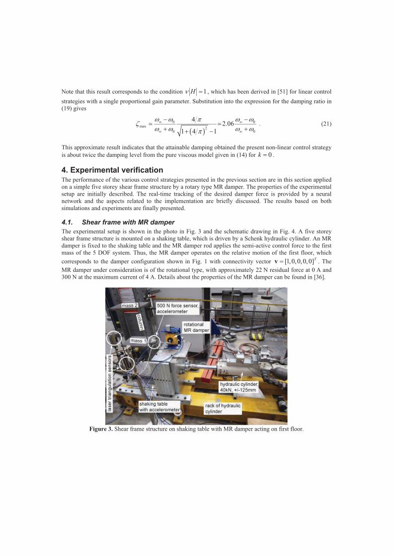
Note that this result corresponds to the condition 1H� � , which has been derived in [51] for linear control
strategies with a single proportional gain parameter. Substitution into the expression for the damping ratio in
(19) gives
� �
0 0max
20 0
42.06
1 4 1
� � � ��
� � � ��
� �
� �
� �
� �� �
� � . (21)
This approximate result indicates that the attainable damping obtained the present non-linear control strategy
is about twice the damping level from the pure viscous model given in (14) for 0k � .
4. Experimental verification
The performance of the various control strategies presented in the previous section are in this section applied
on a simple five storey shear frame structure by a rotary type MR damper. The properties of the experimental
setup are initially described. The real-time tracking of the desired damper force is provided by a neural
network and the aspects related to the implementation are briefly discussed. The results based on both
simulations and experiments are finally presented.
4.1. Shear frame with MR damper The experimental setup is shown in the photo in Fig. 3 and the schematic drawing in Fig. 4. A five storey
shear frame structure is mounted on a shaking table, which is driven by a Schenk hydraulic cylinder. An MR
damper is fixed to the shaking table and the MR damper rod applies the semi-active control force to the first
mass of the 5 DOF system. Thus, the MR damper operates on the relative motion of the first floor, which
corresponds to the damper configuration shown in Fig. 1 with connectivity vector T]0,0,0,0,1[�v . The
MR damper under consideration is of the rotational type, with approximately 22 N residual force at 0 A and
300 N at the maximum current of 4 A. Details about the properties of the MR damper can be found in [36].
Figure 3. Shear frame structure on shaking table with MR damper acting on first floor.

Figure 4. Schematic of test setup.
The accelerations of all five structure masses and the ground acceleration are recorded by accelerometers
from PCB. Furthermore, the absolute displacement of the shaking table, the first floor and the fifth floor are
recorded by laser distance sensors from Micro-Epsilon. Hereby, the acceleration and displacement of the MR
damper motion can be obtained in real-time as the difference between the first floor acceleration and
displacement and the acceleration and displacement of the shaking table, respectively. The control strategies
require real-time estimation of the damper velocity. This is obtained via the measured relative displacement
and acceleration through a Kinematic Kalman Filter (KKF), which is explained in detail in [52]. Finally, a
force sensor is installed between the MR damper rod and the first floor plate in order to measure the damper
force real-time. This force signal is used to determine the tracking error of the implemented control
strategies.
The control of the MR damper is programmed and implemented in Matlab/dSPACE®, which is also used
for the data acquisition. The real-time loop implemented for both the experimental and the numerical
analysis is shown in Fig. 7, where the bottom part shows the control implementation. The output of this
control algorithm is the desired damper force at a sampling frequency of 500 Hz. The desired current is
converted into a command voltage, which is passed through the IO board to the KEPCO current driver,
which provides a negligible tracking error of the desired MR damper current. The Matlab/Simulink® file of
the controller is simultaneously used to compute the command voltage for the INSTRON control unit, which
controls the motion of the hydraulic cylinder. In the simulations the response of the shear frame structure is
determined by integration of the equation of motion in (1), where the MR damper force is governed by a
Bouc-Wen type model. In Fig. 7 these elements are contained in the upper right part of the diagram.

Figure 5. Real-time implementation of semi-active control in Matlab/dSPACE®.
4.2. Implementation of semi-active control The semi-active control of the MR damper is contained in the bottom part of the diagram in Fig. 7. The input
to the control part is the displacement and the velocity of the damper. In the experiments the displacement is
directly measured, while the velocity is determined by the KKF. The box “Control Law” computes the
desired damper force by (9) for the linear models and (15) for the non-linear model. In (15) the amplitude X
is simply the magnitude of the most recent minimum or maximum in the damper displacement response.
Thus, (15) is implemented as an adaptive scheme, which has been used in e.g. [34,46,53] for control of
friction and MR type dampers.
The desired control is then passed on to the “Clipping” box, where any non-dissipative force components
are simply removed. The logic is
: 0
0 : 0
des des
des
des
f f xf
f x
��� �
��
��
(22)
whereby any non-dissipative forces are set to zero.
The absolute values of the desired damper force and the damper velocity are passed on to the force
tracking box, which is denoted “Validated Neural Network of Inverse MR Damper Behaviour” in Fig. 7. The
model-based force tracking without feedback from a force sensor is in this case based on an inverse neural
network model of the MR damper. The input to the neural network is the absolute value of the damper
velocity x� and the absolute value of the desired damper force desf . The output of the neural network is the
associated desired MR damper current desI . The input-output relation of the neural network ( NN ) is
modelled by the following architecture, where details can be found in [39],
( ) ( 1) ( 2) ( 3)
( )( ) ( 1) ( 2) ( 3)
des
des des des des
x j x j x j x jI j NN
f j f j f j f j
� �� � �� � �
� � �� �
� � � � . (23)
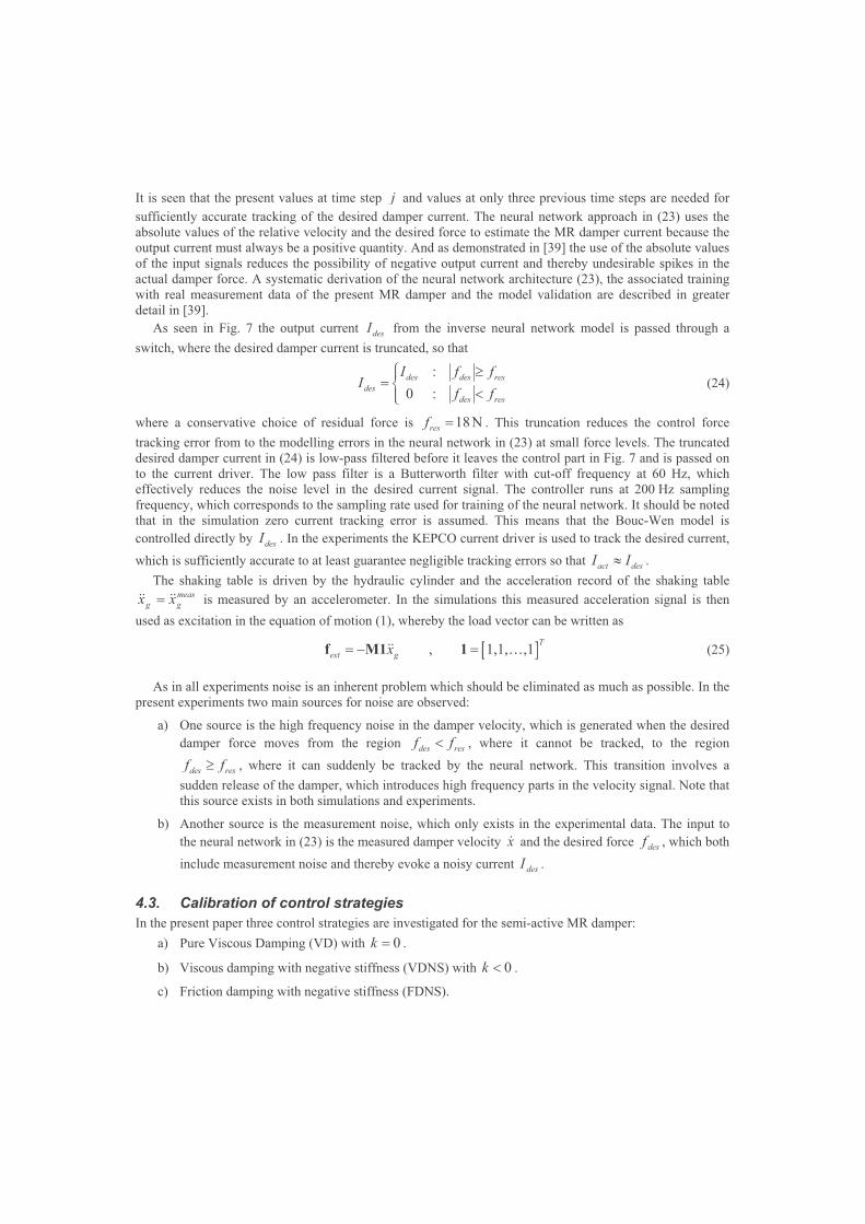
It is seen that the present values at time step j and values at only three previous time steps are needed for
sufficiently accurate tracking of the desired damper current. The neural network approach in (23) uses the
absolute values of the relative velocity and the desired force to estimate the MR damper current because the
output current must always be a positive quantity. And as demonstrated in [39] the use of the absolute values
of the input signals reduces the possibility of negative output current and thereby undesirable spikes in the
actual damper force. A systematic derivation of the neural network architecture (23), the associated training
with real measurement data of the present MR damper and the model validation are described in greater
detail in [39].
As seen in Fig. 7 the output current desI from the inverse neural network model is passed through a
switch, where the desired damper current is truncated, so that
:
0 :
des des res
des
des res
I f fI
f f
� ��� �
��� (24)
where a conservative choice of residual force is 18Nresf � . This truncation reduces the control force
tracking error from to the modelling errors in the neural network in (23) at small force levels. The truncated
desired damper current in (24) is low-pass filtered before it leaves the control part in Fig. 7 and is passed on
to the current driver. The low pass filter is a Butterworth filter with cut-off frequency at 60 Hz, which
effectively reduces the noise level in the desired current signal. The controller runs at 200 Hz sampling
frequency, which corresponds to the sampling rate used for training of the neural network. It should be noted
that in the simulation zero current tracking error is assumed. This means that the Bouc-Wen model is
controlled directly by desI . In the experiments the KEPCO current driver is used to track the desired current,
which is sufficiently accurate to at least guarantee negligible tracking errors so that act desI I� .
The shaking table is driven by the hydraulic cylinder and the acceleration record of the shaking table meas
gg xx ���� � is measured by an accelerometer. In the simulations this measured acceleration signal is then
used as excitation in the equation of motion (1), whereby the load vector can be written as
, 1,1, ,1T
ext gx� � �f M1 1�� � (25)
As in all experiments noise is an inherent problem which should be eliminated as much as possible. In the
present experiments two main sources for noise are observed:
a) One source is the high frequency noise in the damper velocity, which is generated when the desired
damper force moves from the region des resf f� , where it cannot be tracked, to the region
des resf f� , where it can suddenly be tracked by the neural network. This transition involves a
sudden release of the damper, which introduces high frequency parts in the velocity signal. Note that
this source exists in both simulations and experiments.
b) Another source is the measurement noise, which only exists in the experimental data. The input to
the neural network in (23) is the measured damper velocity x� and the desired force desf , which both
include measurement noise and thereby evoke a noisy current desI .
4.3. Calibration of control strategies In the present paper three control strategies are investigated for the semi-active MR damper:
a) Pure Viscous Damping (VD) with 0k � .
b) Viscous damping with negative stiffness (VDNS) with 0k � .
c) Friction damping with negative stiffness (FDNS).

The first two linear models are given in (9), while the friction model with negative stiffness is determined by
the expression in (15). It should of course be noted that all strategies are clipped and truncated according to
the diagram in Fig. 7. Since negative stiffness in the linear model VDNS results in active force components,
it is expected that this model is clipped extensively. The non-linear FDNS also contains a negative stiffness
component. However, the friction term is adaptively scaled with respect to the response amplitude X , and
the stiffness term is balanced by k� � � . This means that clipping is effectively reduced by the non-linear
control model. The model calibration of the shear frame structure is described in Appendix A, and based on
the estimated mass and stiffness matrix the two limiting frequencies and the modal scaling parameter
associated with the first vibration mode are determined as 4
0 8.0 rad/s , 10.4 rad/s , 1.5410� � � �
�� � �
For the pure VD model the damper parameter (13) and the estimated damping ratio (14) are obtained as
max max650 Nm/s , 0.13c � �
For the VDNS model with 4.5kN/mk � � the values are
max max590 Nm/s , 0.43c � �
It should be noted that the apparent stiffness of the bottom storey is approximately 9.5 kN/m, and the
magnitude of the negative stiffness component corresponds to about half of this inter-storey stiffness. The
negative stiffness results in a slight reduction of the viscous parameter, while the estimate of the damping
ratio indicates a significant increase in damping. For the non-linear FDNS model in (15), which is composed
of friction and negative stiffness, the damper parameter is determined by (20) and the corresponding estimate
of the damping ratio is given in (21),
max4kN/m , 0.27� � �
It is observed that the value of � is of the same order of magnitude as the negative stiffness component used
for VDNS. The estimated damping ratio by the non-linear control model is a factor two larger than for pure
viscous damping, but not nearly as high as for the VDNS. However, as indicated by the experimental and
numerical results presented in the following the clipping of the active parts of the linear VDNS leads to a
significant deterioration of the expected performance and thus a change in the calibration. Because the non-
linear FDNS is adaptively controlled proportional to the response amplitude the clipping is significantly
reduced and the expected performance is almost recovered in the experiments, as demonstrated in the
following sections.
4.4. Force tracking The force tracking error is in this case illustrated for the pure VD in Fig. 6. The results are for a maximum
force level of approximately 60 N, which is a typical value for the first mode of the present shear frame
structure. Figures 6a,b show the force tracking and the corresponding current signal for the experiment,
while Figs. 6c,d show the similar results for the simulations. It is seen that the force tracking error in the
experiment is slightly larger than in the simulation, which is mainly due to measurement noise in the
collocated velocity which generates a noisy current. Note that because the MR damper behaves as a low-pass
filter the actual damper force is not as noisy as the damper current. By comparison with the simulations in
Fig. 6c it is found that the noise level in the experimental record in Fig. 6a is acceptable. Both time histories
show the regions of the residual force that constrains the force tracking. Within these regions zero current is
applied in order to minimize the force tracking error.

Figure 6. Measured (a,b) and simulated (c,d) force tracking of viscous damper force.
Figure 7. Measured (a,b) and simulated (c,d) force-displacement and force-velocity trajectories for pure VD.
4.5. Steady-state response The performance of the control strategies for the rotational MR damper is assessed at steady-state and
harmonic conditions and by free vibration decay. For the pure VD the force-displacement and force-velocity
trajectories are shown in Fig. 7. It is seen that the force tracking is fairly accurate, where the main tracking

error is due to the residual force level at 0 A, where the MR damper basically operates as a friction damper.
Thus, inside this region deviations from the ideal viscous ellipse are expected and observed. Furthermore, the
level of experimental noise can be evaluated by comparison with Fig. 7c,d, which show the corresponding
simulation results.
Figure 8. Steady-state response and free decay for pure VD.
Figure 8 shows the response of the top floor, where Fig. 8a is the experimental response and Fig. 8b is
obtained by simulations. The amplitude and root-mean-square ( rms ) values are determined during steady-
state conditions. As indicated in Fig. 8 the harmonic excitation by the shaking table is suddenly stopped and
the free vibration decay provides an estimate of the damping ratio. Due to the fairly large damping the
number of local peaks with non-zero MR damper current is quite limited. This means that the estimation of
the damping ratio is quite difficult. The point-to-point estimate of the damping ratio by logarithmic
decrement is shown by the crosses in Fig. 8, and an average value is used to generate the exponential fit also
shown in the figure. The average damping ratio is given in Table 1, and for the VD it is 0.12, which is quite
similar to the expected value of 0.13 determined in Section 4.3. Details on the estimation of the damping
ratio can be found in [34]. The damper parameters presented in Table 1 are determined by trial-and-error,
and represent the damper parameters that lead to the largest average damping ratio in the free vibration decay
experiments. For the pure viscous damper the experimentally determined damper parameter agrees very well
with the theoretical estimated determined in Section 4.3.
Table 1. Measured and simulated mean damping ratios and steady state responses.
Control law VD Clipped VDNS FDNS
calibration c =650 Nm/s c =250 Nm/s
k =-4500 N/m
� =3000 N/m
mea
sure
d
[%] 11.8 approx. 22 approx. 26
)( 5xrms [mm] 24.3 15.5 11.2
)( 1xrms [mm] 6.6 4.9 3.5
)( 5xrms �� [m/s2] 1.81 1.25 1.02
)( 1xrms �� [m/s2] 0.87 1.02 0.94
sim
ula
ted
[%] 13.4 approx. 30 approx. 30
)( 5xrms [mm] 24.3 (*) 13.8 13.6
)( 1xrms [mm] 6.1 6.3 5.5
)( 5xrms �� [m/s2] 1.60 0.98 1.16
)( 1xrms �� [m/s2] 0.64 1.40 1.36

In addition to the mean damping ratio, the damping performance of the tested control concepts is also
assessed by the root mean square of the steady state response at constant excitation amplitude and the
resonance frequency of the first vibration mode. The rms is determined for the displacement of the first floor
and the top floor. Furthermore, the rms values are computed for the associated acceleration records, where in
particular the acceleration of the first floor relates to the high-frequency content in the damper force. Note
that the undamped case is not reported, since the resonant response without the MR damper will lead to
collapse of the shear frame structure. Thus, the pure VD represents the benchmark case for the two control
models with negative stiffness.
Figure 9 shows the steady-state response and free vibration decay for VDNS. The results for the average
damping ratio and rms are given in Table 1. By the trial and error procedure it has been found that due to the
heavy clipping of the active parts of the damper force associated with the negative stiffness component the
best viscous parameter is reduced from the theoretical value of max 590 Nm/sc � to 250Nm/s . For this
value the damping ratio is around 0.2 � , which is significantly smaller than the estimated value of more
than 0.4 . It is seen from the rms values that the introduction of negative stiffness improves the response
reduction at both top and first floor. However, the increase in first floor acceleration indicates that the high-
frequency content in the damper force also increased. This is furthermore verified by the curves in Fig. 9a,
which show that the strong clipping at the points of reversal in the damper motion results in a very spiky
damper response.
Figure 9. Steady-state response and free decay for clipped VDNS.

Figure 10. Steady-state response and free decay for FDNS.
Figure 10 shows the steady-state response and free vibration decay for the non-linear FDNS. It is seen
that the tracking of the force-displacement trajectory in Fig. 10a is fairly good compared to the case of
VDNS in Fig. 9a. As seen in Table 1 the actual damper value is 3000 N/m� � , which is somewhat smaller
than the estimated value of 4000 N/m . The reason for that is that the attainable force level at 4 A of the MR
damper is not large enough to realize the full potential of the FDNS for the present shear frame structure.
And because the excitation level of the structure has been chosen so that the pure viscous damper is
operating in the full force range, the damper parameter for the FDNS has simply been reduced to
3000 N/m� � . However, the average damping ratio is approximately 0.26 � , which agrees well with
the theoretical prediction of 0.27 . This indicates that effective damping by semi-active devices, in this case
an MR damper, requires control strategies that take the inherent characteristics of the particular damping
device into account. In the present case the negative stiffness in (15) is balanced so that the damper force is
zero at reversal, which is verified by the results shown in Figs. 10a,c. The rms values for the FDNS also
show a significant reduction in the structural response, and the increase in the rms value of the first floor
acceleration is significantly smaller compared to clipped VDNS and it is only slightly larger than the value
for pure VD.
5. Conclusions
The present paper investigates the performance of semi-active control schemes with negative stiffness in
connection with damping of flexible structures by an MR damper. The results and main conclusions are
based on experimental results where a rotational type MR damper is operating on the first floor of a simple
five storey shear frame model structure.
As discussed in the introduction the application of negative stiffness leads to an increase of the local
motion over the damper, and combined with a proper calibration of the associated dissipative damper
component this may result in improved energy dissipation and thereby structural damping. The increased
motion at damper location might lead to an increase in local strains and stresses in the structure. However, as
illustrated by the experiments performed in the paper the increase in damping, due to the introduction of
negative damper stiffness, results in an overall reduction of the MR damper motion, which at least indicates

that for semi-active control the introduction of proper negative stiffness is beneficial for damping of flexible
structures.
Two simple control models are considered for the MR damper: a linear model with a viscous term and a
negative stiffness term, and a non-linear model with a friction term and a negative stiffness term. For the
non-linear term the negative stiffness is balanced so that in harmonic steady-state conditions the damper
force is entirely dissipative. In practice the force level of the friction force is scaled with the value of the
most recent minimum or maximum in the damper displacement record. This adaptive procedure is fairly
simple and also quite accurate in the case of resonant response, where the response amplitude is slowly
varying. Both models are compared to the performance of the pure viscous damper model with vanishing
damper stiffness.
The desired calibration and predicted damping ratio is based on the free vibration analysis of the structure
in Section 2. The derived expression for the modal damping ratio indicates that the introduction of negative
stiffness might lead to an increase in the damping ratio. This is verified by the experiments reported in
Section 4. For the linear damper model a very large damping ratio is predicted by the theory when
1k� � � . However, for negative stiffness the linear model produces non-dissipative, and thereby active,
control forces. In semi-active control these parts are typically clipped, which results in a deterioration of the
theoretical findings. For small values of k� the influence of the negative stiffness is limited and the results
for the pure viscous model are basically recovered, while for k� close to -1 the active parts dominate the
damper force and clipping limits the performance of the damper. The best calibration is most certainly
somewhere between these limits, and the present experiments apply 0.7k� � � , which is a fairly large value.
As observed during the experiments this value leads to a significant amount of clipping, and the best viscous
parameter, found by simple trial-and-error, is less than half the value predicted by the theory. Furthermore,
the damping performance determined by the free vibration decay tests is also significantly less than the
theoretical estimate. This indicates that in connection with semi-active control care must be taken with
respect to clipping of active parts when introducing negative stiffness in a linear damper model.
Since the friction part and the negative stiffness of the non-linear model have been properly balanced by
k� � � , the need for clipping in steady-state conditions is significantly reduced, and the calibration and
corresponding damping performance of this model agree fairly well with the analytical results. In fact, the
mayor discrepancy in the non-linear model seems to be due to the limited force level of the MR damper at 4
A, which implies that the desired damper force cannot be fully realized by the damper. In the experiments
the actual value of � is therefore slightly reduced compared to the analytical estimate in Section 4.3. A
modified version of the present non-linear model could be formulated to take this saturation into account,
whereby the analytical calibration should agree better with the experimental results, obtained by trial and
error. The formulation of such a modified damper model is definitely part of future work on the control of
semi-active dampers.
The experiments and the experimental results are presented in Section 4, where it is explained how the
control loop is implemented in Matlab/dSPACE®. A main issue in the control implementation is the real-
time tracking of the desired control force. This is performed by a simple neural network, where the desired
output current from the neural network is subsequently clipped to avoid non-dissipative forces, truncated to
take care of the 0 A residual force and low-pass filtered to reduce the noise level. Despite these subsequent
modifications of the neural network output the actual MR damper force is still rather spiky. Nevertheless, the
measured structural damping agrees quite well with the simulated values. Thus, the neural network method
represents an effective tool for the modelling of the inverse MR damper dynamics for real-time tracking of a
desired damper force without feedback from a force sensor.
ACKNOWLEDGEMENTS
The work is supported by Empa, Swiss Federal Laboratories for Materials Science and Technology,
Switzerland, by the research grant of the Danish Council of Research and Innovation, Denmark, and by the
industrial partner Maurer Söhne GmbH & Co. KG, Germany.

6. Appendix A
The shear frame structure is shown in Fig1. 1 and 2, and in this appendix the procedure for the modelling of
the structure is briefly described. The horizontal floor displacements represent the five degrees of freedom in
1 2 3 4 5, , , ,T
x x x x x�x . The equation of motion is given (1), introducing the mass matrix M , the damping
matrix C and the stiffness matrix K . These system matrices are determined by the following engineering
type approach:
a) The mass matrix is assumed diagonal, where each component represents the weights of a single floor
mass and four columns.
b) The shear frame is base excited (without MR damper) by a sine sweep, which determines the five
natural frequencies and the corresponding mode shapes.
c) The free decay response of the five vibration modes estimates the modal damping ratios.
The diagonal elements of the mass matrix M are the sum of floor mass and column mass, which gives
( , ) 4 5.95kgmass columnj j m m� � �M
The natural frequencies and mode shapes are estimated from the base sine sweep of the structure. The
response is recorded by the accelerometers on each floor and base, and Fig. A1a,c shows acceleration record
for floors 1 and 4.
Figure A1. Acceleration record from base sine sweep: (a,c) experiments, (b,d) simulations.
From the sine sweep record and by the peaks in the associated power spectrum, Fig.A2, the experimental
angular natural frequencies are determined as
1 2 3 4 58.0 , 24.2 , 38.4 , 49.9 , 58.3� � � � �� � � � �
all in rad/s.

Figure A2. Power spectrum: (a,c) experiments, (b,d) simulations.
The associated vibration forms iu are estimated from the measured transfer functions and by inspection of
the correlation of the minima and maxima in the floor records. The estimated vibration forms are shown in
Fig.A3a, and it is seen that they agree well with the analytical solution for the mode of an ideal shear frame
structure
,
2 1sin
2 1i j
ju i
n�
�! "� # $
�% & (A1)
where i is the mode number, j is the floor number and n is the number of degrees of freedom. It is seen
from Fig. A3a that the agreement between the estimated vibration forms and the analytical expressions is
quite good. The measured mode shape vectors are collected in the matrix 1 n�U u u� , whereby the modal
mass matrix is determined as
T
m �M U MU (A2)
The associated diagonal modal stiffness matrix is determined by multiplication of the diagonal elements of
the modal mass matrix with the square of the natural frequencies,
2( , ) ( , )m i mj j j j��K M (A3)
The back transformation from modal to Cartesian coordinates gives the estimate of the stiffness matrix,
� � � �1 1T
m
� ��K U K U . (A4)
The stiffness matrix is symmetric but not necessary tri-diagonal, as for an ideal shear frame structure.
However, it is found that the off tri-diagonal elements are small compared to the elements in the tri-diagonal
band.

Figure A3. (a) Mode shapes and (b) free vibration decay of shear frame structure.
The modal damping is estimated by free vibration decay tests. Figure A3b shows the top floor displacement
response when the structure is base excited at the natural frequency of the first mode. When the base
excitation is stopped the structure performs free vibration decay in the particular vibration form. By point-to-
point logarithmic decrement [34] the modal damping ratios are determined as
1 2 3 4 50.0030 , 0.0024 , 0.0020 , 0.0015 , 0.0010 � � � � �
When using the estimated modal mass and modal stiffness matrices the diagonal elements of the modal
damping matrix becomes
( , ) 2 ( , ) ( , )m j m mj j j j j j �C K M (A5)
where the off-diagonal elements are assumed to vanish. The damping matrix in Cartesian coordinates is
determined as for the stiffness matrix in (A4). The natural frequencies and the damping ratios of the
estimated model are determined by solving the damped eigenvalue problem associated with the
homogeneous version of the equation of motion in (1). The natural frequencies are
1 2 3 4 58.0 , 24.2 , 38.4 , 49.9 , 58.3� � � � �� � � � �
while the modal damping ratios are
1 2 3 4 50.0010 , 0.0040 , 0.0071 , 0.0055 , 0.0016 � � � � �
It is seen that good agreement is observed for the natural frequencies, while fairly large errors are observed
for the modal damping. The sine sweep response is simulated based on the estimated system matrices, see
Fig. A1b,d. Comparison with the experimental records indicates a deviation in the response magnitude,
which follows from the errors in the damping. This is also observed for the power spectra in Fig. A2.
7. References
[1] Spencer Jr. B F and Nagarajaiah S, 2003, State of the Art of Structural Control, Journal of Structural
Engineering 129(8) 845-56.
[2] Christenson R E, Spencer Jr. B F and Johnson E A, 2006, Experimental Verification of Smart Cable
Damping, Journal of Engineering Mechanics 132(3) 268-78.
[3] Jung H J, Jang J E, Choi K M and Lee H J, 2008, MR fluid damper-based smart damping systems for
long steel stay cable under wind load, Smart Structures and Systems 4(5) 697-710.
[4] Li H, Liu M, Li J, Guan X and Ou J, 2007, Vibration control of stay cables of the Shandong Binzhou
yellow river highway bridge using magnetorheological fluid dampers, Journal of Bridge Engineering
12(4) 401-409.

[5] Maslanka M, Sapinski B and Snamina J, 2007, Experimental study of vibration control of a cable with an
attached MR damper, Journal of Theoretical and Applied Mechanics 45(4) 893-917.
[6] Weber F, Feltrin G and Motavalli M, 2005, Passive damping of cables with MR dampers, Journal of
Materials and Structures 38(279) 568-77.
[7] Weber F, Feltrin G and Motavalli M, 2005, Measured LQG Controlled Damping, Smart Mater. Struct.
14(6) 1172-83.
[8] Weber F, Distl H, Feltrin G and Motavalli M, 2009, Cycle energy control of MR dampers on cables,
Smart Mater. Struct. 18 015005.
[9] Weber F and Boston C, Clipped viscous damping with negative stiffness for semi-active cable damping,
Smart Mater. Struct. 20 (2011) 045007 (13pp).
[10] Wu W J and Cai C S, 2010, Cable vibration control with a semiactive MR damper-numerical simulation
and experimental verification, Structural Engineering and Mechanics 34(5) 611-23.
[11] Aguirre N, Ikhouane F, Rodellar J, Wagg D J and Neild S A, 2010, Viscous and Dahl model for MR
dampers characterization: A Real time hybrid test (RTHT) validation Proceedigns of the 14th
European Conference on Earthquake Engineering, August 30 - September 03, 2010, Ohrid, Republic
of Macedonia.
[12] Cho S-W, Kim B-W, Jung H-J and Lee I-W, 2005, Implementation of Modal Control for Seismically
Excited Structures using Magnetorheological Dampers, Journal of Engineering Mechanics 131(2)
177-84.
[13] Choi K-M, Jung H-J, Lee H-J and Cho S-W, 2008, Seismic protection of base-isolated building with
nonlinear isolation system using smart passive control strategy, Structural Control and Health
Monitoring 15(5) 785-96.
[14] Gattulli V, Lepidi M and Potenza F, 2009, Seismic protection of frame structures via semi-active
control: modeling and implementation issues, Earthquake Engineering and Engineering Vibration
8(4) 627-45.
[15] Gordaninejad F, Saiidi M, Hansen B C, Ericksen E O and Chang F-K 2002 Magneto-Rheological Fluid
Dampers for Control of Bridges, Journal of Intelligent Material Systems and Structures 13(2/3) 167-
80.
[16] He W L, Agrawal A K and Yang J N, 2003, Novel Semiactive Friction Controller for Linear Structures
against Earthquakes Journal of Structural Engineering 1291(7) 941-50.
[17] Jung H-J, Spencer Jr. B F and Lee I-W, 2003, Control of Seismically Excited Cable-Stayed Bridge
Employing Magnetorheological Fluid Dampers, Journal of Structural Engineering 129(7) 873-83.
[18] Lee H J, Jung H J, Moon S J, Lee S K, Park E C and Min K W, 2010, Experimental Investigation of MR
Damper-based Semiactive Control Algorithms for Full-scale Five-story Steel Frame Building, Journal
of Intelligent Material Systems and Structures 21(19) 1025-37.
[19] Lin Y Z and Christenson R, 2011, Real-Time Hybrid Test Validation of a MR Damper Controlled
Building with Shake Table Tests, Advances in Structural Engineering 14(1) 79-92.
[20] Lu K C, Loh C H, Yang J N and Lin P Y, 2008, Decentralized sliding mode control of a building using
MR dampers, Smart Mater. Struct. 17(5) 055006.
[21] Neelakantan V A and Washington G N, 2008, Vibration Control of Structural Systems using MR
dampers and a ‘Modified’ Sliding Mode Control Technique, Journal of Intelligent Material Systems
and Structures 19(2) 211-24.
[22] Pradono M H, Iemura H, Igarashi A, Toyooka A and Kalantari A, 2009, Passively controlled MR
damper in the benchmark structural control problem for seismically excited highway bridge,
Structural Control and Health Monitoring 16(6) 626-38.

[23] Sun Q, Wu XH, Xue XM, Zhang L and Zhang L, 2010, Mechanics performance test of MR damper and
its application in structural seismic response control, International Journal of Applied
Electromagnetics and Mechanics 33(3-4) 1493-1501.
[24] Yoshida O and Dyke S J, 2004, Seismic Control of a Nonlinear Benchmark Building Using Smart
Dampers, Journal of Engineering Mechanics 130(4) 386-92.
[25] Zapateiro M, Karimi H R, Luo N and Spencer B F, 2010, Real-time hybrid testing of semiactive control
strategies for vibration reduction in a structure with MR damper, Structural Control & Health
Monitoring 17(4) 427-51.
[26] Zapateiro M, Karimi H R, Luo N S, Phillips B M and Spencer B F, 2009, Semiactive Backstepping
Control for Vibration Reduction in a Structure with Magnetorheological Damper Subject to Seismic
Motions, Journal of Intelligent Material Systems and Structures 20(17) 2037-53.
[27] Cai C S, Wu W J and Araujo M, 2007, Cable Vibration Control with a TMD-MR Damper System:
Experimental Exploration, Journal of Structural Engineering 133(5) 629-37.
[28] Weber F, Boston C and Ma�lanka M, 201,1 Adaptive TMD based on the emulation of positive and
negative stiffness with MR damper, Smart Mater. Struct. 20 (2011) 015012 (11pp).
[29] Wu W J and Cai C S, 2007, Theoretical exploration of a taut cable and a TMD system Journal of
Engineering Structures 29 962-72.
[30] Zemp R, de la Llera J C and Roschke P, 2011, Tall building vibration control using a TM-MR damper
assembly: Experimental results and implementation, Earthquake Engineering & Structural Dynamics
40(3) 257-71.
[31] Zemp R, de la Llera J C and Almazan JL, 2011, Tall building vibration control using a TM-MR damper
assembly, Earthquake Engineering & Structural Dynamics 40(3) 339-54.
[32] Boston C, Weber F and Guzzella L, 2009, Optimal semi-active damping of cables: evolutionary
algorithms and closed-form solutions, Smart Mater. Struct. 18 055006.
[33] Boston C, Weber F and Guzzella L, 2011, Optimal semi-active damping of cables with bending
stiffness, Smart Mater. Struct. 20 055005 (8pp).
[34] Weber F, Høgsberg J and Krenk S, 2010, Optimal tuning of amplitude proportional Coulomb friction
damper for maximum cable damping, Journal of Structural Engineering 136(2) 123-34.
[35] Dyke S J, Spencer Jr B F, Sain M K and Carlson J D, 1996, Modeling and control of
magnetorheological dampers for seismic response reduction, Smart Mater. Struct. 5(5) 565–75.
[36] Boston C, Weber F and Guzzella L, 2010, Modeling of a disk-type magnetorheological damper, Smart
Mater. Struct. 19 045005.
[37] Jiménez R and Alvarez-Icaza L, 2005, LuGre friction model for a magnetorheological damper, Journal
of Structural Control and Health Monitoring 12 91-116.
[38] Yang F, Sedaghati R and Esmailzadeh E, 2009, Development of LuGre Friction Model for Large-Scale
Magneto-Rheological Fluid Damper, Journal of Intelligent Material Systems and Structures 1 doi:
10.1177/1045389X08099660.
[39] Bhowmik S, Weber F and Høgsberg J, 2011, Experimental calibration of forward and inverse neural
networks for rotary type magnetorheological damper, submitted for publication.
[40] Karamodin A, Kazemi H, 2010, Semi-active control of structures using neuro-predictive algorithm for
MR dampers, Structural Control & Health Monitoring 17(3) 237-53.
[41] Sun W, Hu H and Weng J, 2006, Design, Testing and Modeling of a Magnetorheological Damper with
Stepped Restoring Torque, Journal of Intelligent Material Systems and Structures 17(4) 335-40.

[42] Wang D H and Liao W H, 2005, Modeling and control of magnetorheological fluid dampers using
neural networks, Journal of Smart Materials and Structures 14 111-26.
[43] Xia P, 2003, An inverse model of MR damper using optimal neural network and system identification,
Journal of Sound and Vibration 266 1009-23.
[44] Won J and Sunwoo M, 2003, Fuzzy modelling approach to magnetorheological dampers: forward and
inverse model, Journal of Systems and Control Engineering 20 1055-65.
[45] Tse T and Chang C, 2004, Shear-mode rotary magnetorheological damper for small-scale structural
control experiments, Journal of Structural Engineering 130 904-10.
[46] Høgsberg J, 2009, The role of negative stiffness in semi-active control of magneto-rheological dampers,
Struct. Control Health Monit. DOI: 10.1002/stc.371.
[47] Iemura H and Pradono M H, 2009, Advances in the development of pseudo-negative-stiffness dampers
for seismic response control, Structural Control and Health Monitoring 16(7-8) 784-99.
[48] Li H, Liu M and Ou J P, 2008, Negative stiffness characteristics of active and semiactive control
systems of stay cables, Structural Control &Health Monitoring 15(2) 120-42.
[49] Ou J and Li H, 2010, Analysis of capability for semi-active or passive damping systems to achieve the
performance of active control systems, Structural Control and Health Monitoring 17(7) 778-94.
[50] Main J A and Krenk S, 2005, Efficiency and tuning of viscous dampers on discrete systems, Journal of
Sound and Vibration 286(1-2) 97-122.
[51] Høgsberg J R and Krenk S, 2006, Linear control strategies for damping of flexible structures, Journal of
Sound and Vibration 293(1-2) 59-77.
[52] Jeon S, Tomizuka M and Katou T, 2009, Kinematic Kalman Filter (KKF) for robot end-effector
sensing, Journal of Dynamic Systems, Measurement and Control 131(2) 021010 (8 pp).
[53] Weber F and Boston C, 2010, Energy Based Optimization of Viscous-Friction Dampers on Cables,
Smart Mater. Struct. 19 045025.

P3
(Conference paper)
Neural Network based semi-active control strategy for structural vibration mitigation withmagnetorheological damper
Proceedings of the third ECCOMAS Thematic Conference on Computational Methods inStructural Dynamics and Earthquake Engineering
May 25–28, Corfu, Greece, 2010, 540–553


COMPDYN 2011
3rd ECCOMAS Thematic Conference on
Computational Methods in Structural Dynamics and Earthquake Engineering
M. Papadrakakis, M. Fragiadakis, V. Plevris (eds.)
Corfu, Greece, 25–28 May 2011
NEURAL NETWORK BASED SEMI-ACTIVE CONTROL STRATEGY
FOR STRUCTURAL VIBRATION MITIGATION WITH
MAGNETORHEOLOGICAL DAMPER
SUBRATA BHOWMIK
Department of Mechanical Engineering, Technical University of Denmark
403 Nils Koppens Allé, Lyngby, Denmark 2800
e-mail: [email protected]
Keywords: Magnetorheological damper, neural network, semi-active control.
Abstract. This paper presents a neural network based semi-active control method for a rota-
ry type magnetorheological (MR) damper. The characteristics of the MR damper are de-
scribed by the classic Bouc-Wen model, and the performance of the proposed control method
is evaluated in terms of a base exited shear frame structure. As demonstrated in the literature
effective damping of flexible structures is obtained by a suitable combination of pure friction
and negative damper stiffness. This damper model is rate-independent and fully described by
the desired shape of the hysteresis loops or force-displacement trajectories. The proposed
neural network controller is therefore trained based on data derived from these desired force-
displacement curves, where the optimal relation between friction force level and response
amplitude is determined explicitly by simply maximizing the damping ratio of the targeted vi-
bration mode of the structure. The neural network control is then developed to reproduce the
desired force based on damper displacement and velocity as network input, and it is therefore
referred to as an amplitude dependent model reference control method. An inverse model of
the MR damper is needed to determine the damper current based on the derived optimal
damper force. For that reason an inverse MR damper model is also designed based on the
neural network identification of the particular rotary MR damper. The performance of the
proposed controller is compared to that of an optimal pure viscous damper. The top floor dis-
placement and acceleration of the base excited shear frame structure are selected as the per-
formance parameters of this comparison. It is found by the simulations that the proposed
control design yields a reduction in the structural response compared to the viscous case.

Subrata Bhowmik
2
1 INTRODUCTION
As large scale structures become increasingly slender and flexible the magnitude of dy-
namic response due to loading from wind, traffic and even earthquakes may increase beyond
the acceptable level. Thus, the need for additional external damping is pronounced, where in
particular the concept of semi-active control has received a great amount of attraction during
the most recent decades. The Magnetorheological (MR) damper is one of the most popular
types of semi-active devices. It is inherently dissipative and thereby stable, and it behaves
roughly as a friction damper, where the friction force level can be altered real-time by simply
changing the applied damper current. Thus, the MR damper is a cost effective device that
combines some of the adaptability of active control with the low power requirements and re-
liability of pure passive dampers.
The main challenges arising in connection with the use of most semi active damping de-
vices lies in the development of effective control laws, and in the subsequent digital and real-
time implementation. Most control strategies for semi-active structural control fall into two
main categories. The first one consists of control strategies that require accurate mathematical
formulation for the plant model. Examples in this category are the H2/LQG, H� and the slid-
ing mode control, where any active parts are simple clipped. Conversely, the second category
contains control strategies that do not require an accurate mathematical model of the plant.
Neural network and fuzzy control fall into this category. Several neural network based control
strategies [1-3], neuro-fuzzy network based strategies [4,5] or neuro-predictive control me-
thods [6] have been developed for different control aspects of MR dampers. The advantage of
neural network based methods is that they mainly excel in the handling of uncertainties in
nonlinear applications, which makes them suitable for both modeling and control of the inhe-
rently nonlinear MR damper.
It has been demonstrated in [7,8] that for semi-active control of flexible structures the
combination of pure friction and a negative stiffness component yields very effective damping
of structural vibrations. Therefore, this paper considers the development of a model reference
neural network, which will track the desired hysteresis behavior of an ideal friction damper
with negative stiffness. The proposed controller performance is compared with performance
of an optimal viscous damper, and for the response of a simple shear frame structure sub-
jected to harmonic base excitation the good performance of the proposed method is verified.
2 STRUCTURAL MODEL AND MR DAMPER PROPERTIES
The performance of the semi-active control strategies for the MR damper is in this paper
assessed by the harmonic response of a base excited five-storey shear frame structure. The
MR damper is collocated at the first floor of the shear frame, where the measuring data is col-
lected. To apply the semi-active control strategy on the MR damper, an inverse model of the
damper is needed to predict the damper current associated with the desired MR damper force.
The equation of motion of the shear frame structure with MR damper and inverse MR damper
model are discussed in the following sub-sections.
2.1 Equation of motion
In dynamic analysis of flexible structures the structural model is typically modeled by fi-
nite elements or determined by experimental modal analysis, whereby the equation of motion
can be written in the form
� �c c c c gf x� � � � � �M x C x K x � M I�� � �� (1)

Subrata Bhowmik
3
where cM , cC and cK are the mass, damping and stiffness matrices in Cartesian coordinates,
x is the displacement vector containing the displacements of the five concentrated masses,
the dot represents the time derivative, f is the force of the external MR damper,
[1,0,0,0,0]T�� is the connectivity vector that applies the semi-active force f to the first
mass, T]1,1,1,1,1[�I is the unity vector and gx�� is the ground acceleration. The schematic illu-
stration of the shear frame structure with rotational MR damper is shown in Fig. 1.
+ +
Mass 1
Mass 5
Base
x5
x1
xg....
MR Damper
Figure 1: Shear Frame Structure with MR damper
2.2 MR damper model
The rotational MR damper is modeled using the classical Bouc-Wen hysteresis model. The
parameters of the model have been calibrated by experiments, where the damper has been dri-
ven harmonically in a testing machine at various frequency-amplitude combinations. The
modified Bouc-Wen model by Spencer et al. [9] was formulated for the cylindrical type MR
damper. In the present case this model is slightly simplified, mainly because the cylindrical
damper concept has no need for an accumulator chamber, which for the many cylindrical type
dampers introduce an additional stiffness component. Figure 2 shows the close up of the rota-
ry type damper at the Swiss Federal Laboratory of Material Science and Research (EMPA)
and the schematic diagram of the classical Bouc-Wen model. For more information on the
characteristics and modeling of the rotary MR damper please see Boston et al. [10].

Subrata Bhowmik
4
Metallic Housing
MR Fluid inside
Rotational Disc inside
Bouc-Wen
Co
x
F
Figure 2: Rotational MR Damper and Bouc-Wen damper model
The governing equations for the damper force f predicted by the classical Bouc-Wen model
can be written as follows:
� �0f z c x�� � � (2)
where the hysteresis effect follows from the evolutionary variable z controlled by the Bouc-
Wen equation
1
( ) ( )n n
z x z z x z A x' (�
� � � �� � �� (3)
The gain parameters on the hysteresis effect and the viscous effect are in the present case de-
scribed by cubic and linear functions of the applied current, respectively:
2 3
0 0 0,a b c d a bu u u c c c u� � � � �� � � � � � (4)
The applied current u is described with a time delay relative to the desired current I by the fol-
lowing first order filter:
( )u u i)� � �� (5)
The estimated parameters of the simplified Bouc-Wen model for the rotational MR damper
are given in Table. 1.
MR Damper Parameters
a� 4.038 ) 100
b� 1.984 ' 410
c� 7.901 ( 410
d� -0.704 A 1000
0ac 10 0bc 100
Table 1: Parameters for Bouc-Wen Model
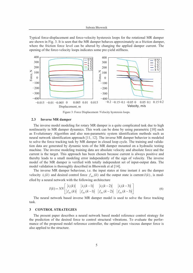
Subrata Bhowmik
5
Typical force-displacement and force-velocity hysteresis loops for the rotational MR damper
are shown in Fig. 3. It is seen that the MR damper behaves approximately as a friction damper,
where the friction force level can be altered by changing the applied damper current. The
opening of the force-velocity loops indicates some pre-yield stiffness.
−0.015 −0.01 −0.005 0 0.005 0.01 0.015
−400
−300
−200
−100
0
100
200
300
400
Displacement, m
Forc
e, N
0 V1 V2 V3 V4 V
−0.2 −0.15−0.1 −0.05 0 0.05 0.1 0.15 0.2−400
−300
−200
−100
0
100
200
300
400
Velocity, m/s
Fo
rce,
N
0 V1 V2 V3 V4 V
Figure 3: Force Displacement /Velocity hysteresis loops.
2.3 Inverse MR damper
The inverse model modeling for rotary MR damper is a quite complicated task due to high
nonlinearity in MR damper dynamics. This work can be done by using parametric [10] such
as Evolutionary Algorithm and also non-parametric system identification methods such as
neural network identification approach [11, 12]. The inverse MR damper behavior is modeled
to solve the force tracking task by MR damper in closed loop cycle. The training and valida-
tion data are generated by dynamic tests of the MR damper mounted on a hydraulic testing
machine. The inverse modeling training data are absolute velocity and absolute force and the
current is the target. This approach has been chosen because current is always positive and
thereby leads to a small modeling error independently of the sign of velocity. The inverse
model of the MR damper is verified with totally independent set of input-output data. The
model validation is thoroughly described in Bhowmik et al [14].
The inverse MR damper behaviour, i.e. the input states at time instant k are the damper
velocity 1( )x k� and desired control force )(kfdes and the output state is current )(kI , is mod-
elled by a neural network with the following architecture
1 1 1 1( ) ( 1) ( 2) ( 3)
( )( ) ( 1) ( 2) ( 3)des des des des
x k x k x k x kI k NN
f k f k f k f k
� �� � �� � �
� � �� �
� � � � (6)
The neural network based inverse MR damper model is used to solve the force tracking
task.
3 CONTROL STRATEGIES
The present paper describes a neural network based model reference control strategy for
the prediction of the desired force to control structural vibrations. To evaluate the perfor-
mance of the proposed model reference controller, the optimal pure viscous damper force is
also applied to the structure.

Subrata Bhowmik
6
For linear damper models the characteristics of the damper are conveniently formulated in
the frequency domain as
( ) ( )f gH x� �� (7)
where g is the control gain and ( )H � is the associated frequency dependent transfer function.
The effective damping of the structure is evaluated in terms of its modal damping ratio,
where the presence of the external damper generates a non-proportional damping with corres-
ponding complex valued natural frequencies and mode shapes. The analysis of the damper
modal vibrations is described by the two-component system reduction technique introduced
by Main and Krenk [13]. In that formulation the response of the structure is represented by a
linear combination of the two limiting mode shapes for the structure without damper 0u and
for the structure with the damper fully locked �u , respectively. The linear combination can
then be written as:
0 0 r r � �� �x u u (8)
The first term represents the classical undamped case, while the second term introduces the
local effect of the damper described in terms of its ability to lock the structure at its location.
The undamped mode shape is governed by the classical generalized eigenvalue problem
� �2
0 0� � �K M u 0 (9)
A similar eigenvalue problem exists for the case where the damper link is fully locked, de-
fining �� and u�. The locked mode shape �u is by construction orthogonal to the connectivity
vector which yields the identity T
�� u =0.
The two-component representation reduces the full dimensional problem to a two-
dimensional problem, where the associated characteristic equation can be solved explicitly,
providing expressions for the complex valued natural frequency and the corresponding modal
damping ratio. Optimal calibration of the damper model is based on the maximization of the
damping ratio. For the general damper format in (7) it is demonstrated in [14] that the optimal
gain can be determined by the expression:
� �2 2
0
2
0
1optg
H u
� �� ��
(10)
where u0 is the amplitude of the undamped mode shape at damper location. This expression is
in the following used to calibrate the control strategies.
3.1 Viscous damping strategy
The prototype damper model is the pure viscous model. For this model the damper force is
directly proportional to the collocated velocity of the damper motion,
f cx� � (11)
where c is the viscous parameter. When compared with the linear frequency representation of
the damper force in Eq. 7, the damper transfer function for the viscous damper is
0( )H i i� � �� �
(12)
while the gain value is g c�
(13)

Subrata Bhowmik
7
Substitution of (12) and (13) into (10) gives the following expression for the optimal viscous
parameter:
� �0
2
0
2optc
u
� �� ��
(14)
where 0 02� � �� � �
The optimal viscous damper is without stiffness and is therefore a suitable benchmark ex-
ample for damper models with negative stiffness.
3.2 Proposed Neural network based model reference control strategy
The proposed controller is developed based on a neural network model identification tech-
nique, where the neural network model is trained by a reference damper model. In this paper,
the characteristics of the damper model are described by the desired shape of the hysteresis
loop, which combines an amplitude dependent friction damper with a negative stiffness com-
ponent. The optimal shape of this hysteresis loop has originally been identified and verified
by Boston et al. [7]. The hysteresis loop is based on the assumption of pure harmonic dis-
placement and velocity, which is used as the input to the proposed neural model, while the
damper force based on the desired hysteresis loop is used as the output of the neural controller.
The optimal shape of the force-displacement trajectory is shown in fig. 4.
x
-f
f m12
(1 - )mfx
A-
12
(1 + )mfx
A
Figure 4: Force-Displacement Hysteresis model for Friction Damper with negative stiffness
The hysteresis model is inherently nonlinear, whereas the calibration formulation in (10) re-
quires a linear damper model. Thus, an equivalent linear model is assumed to contain a visc-
ous and a stiffness component,
f cx kx� �� (15)
If x is a sinusoidal signal, the parameters of the linear equivalent model in (15) can be deter-
mined by equivalence over a full vibration period, see [14]. The yields the following equiva-
lent linear model for the hysteresis loop in Fig. 4:
m m2-
2
f ff x x
A A��� � (16)
where A is the amplitude of the damper displacement, k is negative stiffness and fm is maxi-
mum force of the hysteresis loop. In frequency domain the model is expressed as
m 1 2
2
ff i x
A �
! "� � �# $
% & (17)

Subrata Bhowmik
8
Comparison with the frequency representation in Eq. 7 gives the following expression for the
transfer function of the linear equivalent hysteretic damper model:
1 2
( )2
H i��
! "� � �# $
% & (18)
and the corresponding gain value:
g =mf
A (19)
From Eq.10 the optimal value of g is determined as
� �2 2
0
2
0
1.24optgu
� �� ��
(20)
The optimal value fm is determined as
m optf g A�
(21)
where A is the amplitude of the displacement.
In this paper, a four-layer feed forward neural network is adopted which consists of one in-
put, two hidden layers and a single output layer. The displacement and velocity with current
state and five preceding values are taken as input and force at current state is output in the
proposed neural network. The neural network controller is trained with training data generated
at different amplitudes and at different frequencies of both the displacement response and the
corresponding force data from the optimal friction model. The trained model is verified with
independent data set and subsequently used in a closed loop implementation. The training al-
gorithm used in the feed forward back propagation neural network is the Levenberg-
Marquardt (LM) algorithm based on a least-square curve fitting.
4 NUMERICAL EXAMPLES
To evaluate the effectiveness of the proposed control strategy for the structural vibration
mitigation with rotary MR damper, two numerical examples are considered. The first one is
based on pure viscous damping strategy and the second one is our proposed neural network
based model reference control (NN-MRC). Both the examples are discussed below
4.1 Viscous Damper
The viscous damping strategy using MR damper in closed loop is simulated for five storied
shear frame structure with harmonic base excitation. The force-velocity and force-
displacement hysteresis plots of the damper force and desired force from control law are
compared for optimal viscous damping strategy and the result is quite satisfactory. The force
tracking task by MR damper is quite well. From fig. 3, it is visible that MR damper has a
force limit at zero current. For that reason it is not possible for MR damper to follow the de-
sired force below the force limit at zero current. Here for this damper, force limit is 24 N.

Subrata Bhowmik
9
−5 0 5 x 10⁻³
−50
0
50
Act
ual
Forc
e, N
−0.05 0 0.05
−50
0
50
−5 0 5 x 10⁻³
−50
0
50
Damper Displacement, m
Des
ired
Fo
rce,
N
−0.05 0 0.05
−50
0
50
Damper Velocity, m/s
Figure 5: Force-Displacement and Force Velocity hysteresis diagram for viscous damper
The top floor displacement and damper displacement are shown in fig. 6.
4 4.5 5 5.5 6 6.5 7 7.5 8−8
−6
−4
−2
0
2
4
6
8x 10
−3
Time, S
Dam
per
Dis
pla
cem
ent,
m
4 4.5 5 5.5 6 6.5 7 7.5 8−0.04
−0.03
−0.02
−0.01
0
0.01
0.02
0.03
0.04
Time, S
To
p F
loo
r D
isp
, m
Figure 6: Time history of damper and top floor displacement for viscous damper
The viscous damping strategy is also applied directly on structure without MR damper and
compared the change in performance.

Subrata Bhowmik
10
4.2 Model Reference Neural Controller
The proposed neural control strategy is applied for structural vibration reduction based on
harmonic base excitation using MR damper in closed loop simulation. The Time history of
damper displacement and top floor displacement are shown below.
4 4.5 5 5.5 6 6.5 7 7.5 8
−6
−4
−2
0
2
4
6
x 10−3
Time, S
Dam
per
Dis
pla
cem
ent,
m
4 4.5 5 5.5 6 6.5 7 7.5 8−0.03
−0.02
−0.01
0
0.01
0.02
0.03
Time, S
Top F
loor
Dis
pla
cem
ent,
m
Figure 7: Force-Displacement and Force Velocity hysteresis diagram for neural controller
The hysteresis plots for force-displacement and force-velocity trajectories are shown in
fig.8.
−5 0 5 x 10⁻³
−50
0
50
Act
ual
Forc
e, N
−0.05 0 0.05
−50
0
50
−5 0 5 x 10⁻³
−50
0
50
Damper Displacement, m
Des
ired
Fo
rce,
N
−0.05 0 0.05
−50
0
50
Damper Velocity, m/s
Ideal FD+NSNN Model
Figure 8: Time history of damper and top floor displacement for neural controller
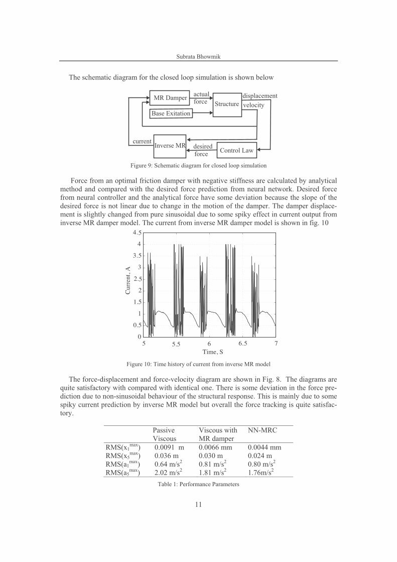
Subrata Bhowmik
11
The schematic diagram for the closed loop simulation is shown below
Structure
Base Exitation
MR Damper displacement
Inverse MR
velocity
Control Lawforce
desired
forceactual
current
Figure 9: Schematic diagram for closed loop simulation
Force from an optimal friction damper with negative stiffness are calculated by analytical
method and compared with the desired force prediction from neural network. Desired force
from neural controller and the analytical force have some deviation because the slope of the
desired force is not linear due to change in the motion of the damper. The damper displace-
ment is slightly changed from pure sinusoidal due to some spiky effect in current output from
inverse MR damper model. The current from inverse MR damper model is shown in fig. 10
5 5.5 6 6.5 70
0.5
1
1.5
2
2.5
3
3.5
4
4.5
Time, S
Cur
rent
, A
Figure 10: Time history of current from inverse MR model
The force-displacement and force-velocity diagram are shown in Fig. 8. The diagrams are
quite satisfactory with compared with identical one. There is some deviation in the force pre-
diction due to non-sinusoidal behaviour of the structural response. This is mainly due to some
spiky current prediction by inverse MR model but overall the force tracking is quite satisfac-
tory.
Passive
Viscous
Viscous with
MR damper
NN-MRC
RMS(x1max
) 0.0091 m 0.0066 mm 0.0044 mm
RMS(x5max
) 0.036 m 0.030 m 0.024 m
RMS(a1max
) 0.64 m/s2 0.81 m/s
2 0.80 m/s
2
RMS(a5max
) 2.02 m/s2 1.81 m/s
2 1.76m/s
2
Table 1: Performance Parameters
Subrata Bhowmik
12
5 CONCLUSIONS
In the closed loop simulation, two neural network models are used. One is for force track-
ing which is an inverse MR damper model and another is used for tracking reference damper
model which is following hysteresis force-displacement behaviour for optimal friction damper
with negative stiffness. RMS of the peak displacement and peak acceleration of each cycle for
top floor and damper location are taken as performance parameters. From the performance
parameters chart, it is clearly visible that proposed control method can reduce around 35% in
damper displacement and 30% in top floor displacement. The damper displacement for visc-
ous damping strategy with and without MR damper has deviation due to limitation MR dam-
per force realization at zero current when MR damper is attached. The response of the top
floor using semi active neural controller gives is quite satisfactory with compared to pure
viscous damping. There is also significant improvement in acceleration term and but the acce-
leration contains some noise. The major advantage of the proposed controller is it is inherri-
tently modeled with amplitude dependency and the inherent time-delay problem which is an
important drawback of model based control can be solved in neural based control. In general,
a neural network is trained under certain condition which can be used in a slightly modified
but similar nature of the training state. The important feature of neural network is that it can
handle nonlinearity so well that it can apply to nonlinear structural control also based on li-
nearly trained neural model. This is the reason why neural network is used in this paper for
structural control. The numerical study revealed that proposed neural based model reference
controller can track the desired hysteresis behaviour of optimal friction damper with negative
stiffness satisfactorily and the performance is better than optimal viscous damper.
ACKNOWLEDGEMENT
This research is financially supported by the Danish Agency for Science, Innovation and
Research. The major part of the work has been done at Swiss Federal laboratory for Material
Science and Research, Switzerland with collaboration with Dr. Felix Weber. These supports
are gratefully acknowledged.
REFERENCES
[1] Z.D. Xu, Y.P. Shen, Y. Q. Guo, Semi-active control of structures incorporated with
magnetorheological dampers using neural network. Smart materials and Structure, 12,
80-87, 2003.
[2] K.A. Bani-Hami, M.A. Sheban, Semi-active neuro-control for base-isolation system us-
ing magnetorheological (MR) dampers. Earthquake Engineering and Structural Dy-
namics, 35, 1119-1144, 2006.
[3] D.H. Kim, S.N. Seo, I. W. Lee, Optimal neurocontroller for nonlinear benchmark struc-
ture. Journal of Engineering Mechanics, 130, 424-429, 2004.
[4] Z.Q. Gu, S.O. Oyadiji, Application of MR damper in structural control using ANFIS
method. Computers and Structures, 86, 427-436, 2008.

Subrata Bhowmik
13
[5] Z.D. Xu, Y. Q. Guo, Neuro-fuzzy control strategy for earthquake-exited nonlinear mag-
netorheological structures. Soil Dynamics and Earthquake Engineering, 28, 717-727,
2008.
[6] A.K. Karamodin, M.H. Kazemi, Semi-active control of structures using neuro-
predictive algorithm for MR dampers. Structural Control and Health Monitoring, DOI:
10.1002/stc.278, 2008.
[7] C. Boston, F. Weber, L. Guzzella, Optimal semi-active damping of cables: evolutionary
algorithms and closed-form solutions, Smart Material and Structures, 18, 055006 (9 pp),
2009
[8] H. Iemura, M.H. Pradono, Advances in the development of pseudo-negative-stiffness
dampers for seismic response control, Structural Control & Health Monitoring, 16,
784-799, 2009
[9] B.F. Spencer, S.J. Dyke, M.K. Sain, J.D. Carlson, Phenomenological model for magne-
torheological dampers. Journal of Engineering Mechanics, 123, 230-238, 1997.
[10] C. Boston, F. Weber, L. Guzzella, Modeling of a disc-type magnetorheological damper,
Smart Material and Structures, 19, 045005 (12 pp), 2010
[11] H. Metered, P. Bonello, S. Oyadiji, The experimental identification of magnetorheolog-
ical dampers and evaluation of their controllers, Mechanical Systems and Signal
Processing, 24, 976-994, 2010
[12] S.Bhowmik, J. Høgsberg, F. Weber, Neural Network Modeling of forward and inverse
behaviour of rotary MR damper. 23rd
Nordic Seminar on Computation Mechanics
(NSCM23), Stockholm, Sweden, October 14-15, 2010.
[13] J.A. Main, S. Krenk, Efficiency and tuning of viscous dampers on discrete systems,
Journal of Sound and vibration, 286, 97-122, 2005
[14] J. Høgsberg, Modeling of Dampers and Damping in Structures, PhD Thesis, Technical
University of Denmark, 2005


P4
(Conference paper)
Semi-active control of magnetorheological dampers with negative stiffness
Proceedings of the fourth ECCOMAS Thematic Conference on Smart Structures andMaterials
July 13–15, Porto, Portugal, 2009, 581–590

1 INTRODUCTION
Survival of structures from excessive vibration due to uncontrollable events—environmental
and otherwise—is of great importance, where vibration control of large flexible structures, such
as building or bridges, is installed primarily to reduce transverse deflections and/or accelera-
tions. Some success toward this goal has been reported in the use of actively controlled devices
like for instance active mass dampers. However, relatively large power requirement is a primary
drawback for this type of structural control. On the other hand, variable or semi-active damping
devices exhibit relatively low power demands and show performance abilities similar to those of
active control schemes (Dyke 1996). In the category of semi-active control, simple variable
damping devices such as magneto-rheological (MR) damper, have received great attention in the
civil engineering community. The MR damper is typically produced in cylindrical form filled
with an MR fluid and surrounded by one or more electromagnetic coils. The fluid contains very
small magnetically polarizable particles that allow the properties of the fluid to change almost
instantaneously according to the strength of the applied magnetic field. A detailed description of
MR dampers can be found in Spencer (1997) or Yang et al. (2001). The application of MR dam-
Semi-active Control of Magneto-Rheological Dampers with
Negative Stiffness
Subrata Bhowmik Department of Mechanical Engineering, Technical University of Denmark, Lyngby, Denmark
Jan Høgsberg Department of Mechanical Engineering, Technical University of Denmark, Lyngby, Denmark
ABSTRACT: Effective damping of large and flexible structures by semi-active dampers relies
greatly on the control strategy applied, which should combine the robustness of passive devices
and the increased damping performance often available from active control. For structural con-
trol the Magneto-rheological (MR) damper is among the most popular and promising devices
due to its low power requirement, high dynamic range, high force capacity and robustness. The
objective of this paper is to formulate semi -active feedback control methods based on simple
linear damper models, which lead to increased damping performance by introduction of appar-
ent negative damper stiffness. The design of the control strategy aims at maximizing the damp-
ing ratio of the critical mode of the structure. Explicit solutions for the complex valued natural
frequency of the damped structure and the associated damping ratio are obtained by the two-
component system reduction technique, which shows that a potential increase in damping is as-
sociated with a similar reduction of stiffness, or even with the introduction of negative stiffness.
For linear control strategies negative stiffness can only be realized by active control, which is
limited by stability. In the present paper it is realized by having the MR damper force track the
simple pure viscous damper model with vanishing stiffness and the Kelvin model with negative
stiffness. The applied voltage of the MR damper should be controlled in such a way that the de-
sired control force is followed sufficiently accurate. This is done by letting the desired force be
the input to an inverse Bingham model, which provides the corresponding desired voltage level
of the MR damper. Numerical simulations are conducted to demonstrate the performance of the
proposed semi-active control strategy with apparent negative stiffness.

pers to the control of vibration has been applied for mitigation of wind and seismic effects on
tall buildings by e.g. Zhang and Roschke (1999) or Jansen and Dyke (1999). An important bene-
fit of an MR damper is its capacity to operate from a remote power source, like a battery or a so-
lar panel, thus increasing its viability during destructive environmental events.
Because of the increasing research in and development of new semi-active devices, the asso-
ciated formulation of suitable control algorithms is of great importance. Two decades ago Yang
et al. (1986) proposed new optimal control algorithms for structural control using standard qua-
dratic performance and Ricccati equation to generate appropriate force. Within the framework
related to linear quadratic Gaussian, H2 or H� control a number of promising approaches have
been presented and have lead to the development and implementation of e.g. sliding mode con-
trol algorithms. Lately, soft computing techniques, for instance based on fuzzy logic theory,
have received some attention. However, the efficiency of these techniques is still to be demon-
strated.
In the present paper two main objectives are considered. Initially a framework for design of ex-
ternal dampers is presented. This is based on the maximization of the damping ratio of a critical
vibration form and it follows the two-component reduction technique presented by Main and
Krenk (2005). This analysis provides expressions for the modal damping ratio, which indicates
that effective damping can be obtained by imposing apparent negative stiffness. Expressions for
optimal tuning of the simple pure viscous damper model and the Kelvin model with negative
stiffness are presented. The second step of the paper considers the realization of the desired con-
trol force, where the applied voltage is obtained in terms of the desired control force by a simple
inverse Bingham plasticity model. A numerical study is presented where the performance of the
introduced semi-active control schemes are evaluated based on the response of a 10 story shear
frame structure exposed to the El Centro earthquake.
2 MODELING OF MAGNETO-RHEOLOGICAL DAMPER
The response of MR fluids results from the polarization induced in suspended particles by appli-
cation of an external magnetic field. The interaction between the resulting induced dipoles
causes the particles to form columnar structure, parallel to the applied field. These chain-like
structures restrict the motion of the fluid, thereby increasing the viscous characteristic suspen-
sion. Spencer et al (1997) presented a phenomenological model to analyze the behavior of a
small scale version of a Magneto- rheological (MR) damper. The model is an augmented version
of the classic Bouc-Wen hysteresis model, and it appears to be representative over a large fre-
quency and amplitude range. A schematic diagram of the modified Bouc-wen model is pre-
sented in Fig. 1.
Fig.1. Modified Bouc-wen Model
The equation governing the force f predicted by the modified Bouc-Wen model is as follows:
1 1 0( )f c y k x x� � �� (1)
where the energy dissipation is introduced via the filter

� � 0 0
0 1
1( )y z c x k x y
c c� � � �
�� �� (2)
and the hysteresis effect follows from the evolutionary variable z governed by the Bouc-Wen
equation
1
( ) ( )n n
z x y z z x y z A x y' (�
� � � � � � �� � � � � �� (3)
The following model parameters are typically represented as linear functions of the applied vol-
tage:
1 1 1 0 0 0, ,a b a b a bu c c c u c c c u� � �� � � � � � (4)
where the applied voltage u is described with a time delay relative to the desired voltage v
( )u u v)� � ��
(5)
Representing the dynamics involved in reaching rheological equilibrium and in driving the elec-
tromagnet in the MR damper, a total of fourteen model parameters are to characterize the MR
damper using experimental data and e.g. a constrained nonlinear optimization algorithm. Taking
displacement, velocity and voltage as input, the model can determine the damper force quite ac-
curately. But due to the nonlinearities of the model its inverse is non-trivial. Therefore, the sim-
ple Bingham plasticity model
a b a bf f f v sign x c c v x� � � �� � (6)
is used to obtain the voltage based on a desired control force, which is derived in the following.
Governing parameters for a 1000 kN MR damper for both the Bingham and the modified Bouc-
Wen model are given in [2]. These parameters are presented in table 1. It should be noted that
the saturation voltage level is around 10 V and that the maximum damper stroke is 0.08 m.
3 DAMPING OF FLEXIBLE STRUCTURES In dynamic analysis of flexible structures the structural model is typically modeled by finite
elements, whereby the equation of motion can be written in the well known form
( )e f t� � � �Mq Cq Kq f w�� � (7)
where the vector q contains the generalized displacements and a dot denotes time differentia-
tion, and K, C and M are the structural stiffness, damping and mass matrix respectively. The ex-
ternal load is represented by the vector process ef . Finally, a single damper is acting on the
structure, where f represents the damper force and w is the connectivity vector describing the
location of the damper. In a collocated setting the displacement of the damper is Tx � w q . The
characteristics of the damper are conveniently formulated in the frequency domain as
( ) ( )f H x� �� (8)
Where H is the frequency dependent transfer function which also contains any damper gain.
The effective damping of the structure is evaluated in terms of its modal damping, where the
presence of the external damper generates non-proportional damping with complex valued natu-
ral frequencies and mode shape. The two-component system reduction technique by Main and
Krenk [3] describes the response as a linear combination of two limiting mode shapes for the
structure without damper 0u and for the structure with the damper fully locked �u , respectively.
0 0 r r � �� �q u u (9)

Bingham Model
fa 100.0 kN fb 75.0 kN/V ca 81.0 kN s/m cb 90.0 kN s/m/V
Modified Bouc-Wen
�a 46.2 kN/m �b 41.2 kN/m/V c0a 110.0 kNs/m c0b 114.3 kNs/m/V
c1a 8359.2kNs/m c1b 7482.9 kNs/m/V k0 0.002 kN/m k1 0.0097 kN/m
x0 0.18 m � 100 1s� � 164.0
2m� � 164.0
2m�
A 1107.2 n 2 Table1: MR damper parameters
The first term represents the classical undamped case, while the second term introduces the local
effect of the damper described in terms of its ability to lock the structure at its location. The un-
damped mode shape is governed by the classical eigenvalue problem
� �2
0 0� � �K M u 0 (10)
A smaller eigenvalue problem exists for the case where the damper link is fully locked, defining
�� and u�. The locked mode shape �u is by construction orthogonal to the connectivity vector
which yields the identity T
�w u =0. Both limiting mode shapes are real-valued and conveniently
normalized to unit modal mass,
T T
0 0 1 , 1� �� �u Mu u Mu (11)
Consequently, the limiting natural frequencies are given in terms of the modal stiffness,
T 2 T 2
0 0 0 , � � �� � � �u Ku u Ku (12)
The limiting mode shapes and natural frequencies are all real-valued and may be derived direct-
ly from the associated generalized eigenvalue problems.
The equations of motion can be described in the reduced two-dimensional subspace by substitu-
tion of (9) into (7) followed by pre-multiplication by the limiting mode-shapes, see e.g.
Høgsberg and Krenk (2006, 2007). In the frequency domain the reduced system of equations
can be written in the following homogeneous form when free vibrations are considered
2 2 2 2 200 0 0
2 2 2 2
0
0( )
0( )
ru H
r
� � * � �
* � � � � ��
� �� � � � � � ��� � � � � �
� � � �� �� � (13)
The amplitude of the mode shape at damper location is 0 0
Tu � w u and 0
T* �� u Mu represents
the coupling between the two limiting mode shapes. Free vibrations require a singular matrix
which yields a characteristic equation in � in e.g. Main and Krenk (2005). This characteristic
equation can be re-written in an explicit, given solution when assuming that the coupling para-
meter 1* � . This solution is conveniently expressed in terms of the change in natural frequency
0� � �+ � � and 0� � �� �+ � � relative to the undamped case, whereby it appears in the fol-
lowing compact form
1
H
H�
+
+ ��� ,
� , (14)
In this expression the modal flexibility parameter is given as
2 2
0 0
2 2
0 02
u u
� �
�� +
�,� � � � (15)
The modal damping ratio is determined as the relative imaginary part of the complex valued
natural frequency: Im � ��� + . In the case of response dominated by resonance the
magnitude of the structural is approximately inverse proportional to the damping ratio of the

dominant mode. Thus, a rational and load independent basis for optimal tuning is the maximiza-
tion of the modal damping ratio with respect to the damper gain. If the approximation
0� �� is introduced the damping ratio can be written as
� �
� �� � � �� �0
220
0 0
Im
1 Re[ ] Im
H
H H
�� �+ � �
� � � �� �
�, ��
� , � , �
(16)
It is seen from this expression that the stiffness of the damper � �0Re[ ]H � appears in the de-
nominator of (16). It is therefore observed that a potential increase in the damping ratio is asso-
ciated with a corresponding reduction of damper stiffness. And as demonstrated in Krenk and
Høgsberg (2006) the application of negative stiffness improves the damping efficiency for reso-
nant response conditions. In the present paper simple damper models are considered in the fol-
lowing, with emphasis on the design of models with negative stiffness and the application in a
semi-active control setting. The optimal tuning of the damper is based on maximization of the
damping ratio, which follows from having the variation 0- � .
4 SAMPLE DAMPER MODELS
4.1 Pure Viscous Damper
The prototype damper model is the pure viscous model. For this model the damper force is di-
rectly proportional to the collocated velocity of the damper motion,
Tf c� w q�
(17) where c is the viscous parameter. This means that the damper transfer function is given as
0( )H ic ic� � �� � (18)
where the frequency in the transfer function is approximated by the undamped frequency. Subs-
titution into (16) followed maximization of the damping ratio gives the following expression for
the optimal viscous parameter
2
0
2optc
u
��+� (19)
The optimal viscous damper has vanishing stiffness and is therefore a suitable case of reference
for damper models with negative stiffness.
4.2 Kelvin Model
The general format of a Kelvin type model has both frequency dependent stiffness and viscous
components. However, in the present formulation it is assumed that the governing parameters
are constant, whereby the damper force can be written as
T
df k c� �w q q� (20)
It is assumed that the stiffness is given and that c is the gain value of the model. The transfer
function can be written as
� � dH k ic� �� � (21)
Substitution into (16) gives the damping ratio and maximization of the damping ratio with re-
spect to c leads to the following expression for the optimal viscous parameter of the Kelvin
model.
2
0 0
2 dopt
kc
u
�
��+
� � (22)
where the second term introduces the correction due to damper stiffness.
5 CONTROL STRATEGIES In the present section a control strategy is presented which operates the semi-active MR damper
similar to the optimally tuned simple viscous damper and the viscous damper with constant
stiffness contribution (Kelvin model). The efficiency of the proposed control strategies depends
in the first place on the proper tuning of the simple damper models, which is given in (19) and
(22) and subsequently on the ability of the MR damper to track the desired optimal control
force.
The following steps outline the design procedure used for the design of the proposed control
scheme:
1. Formulate a MR damper model, which should be as detailed and accurate as possible since
it represents the actual damper attached to the structure. Therefore, the modified Bouc-Wen
model is applied in the present setting.
2. Design of an inverse model of the MR damper, which is used to predict the desired voltage
based on the known optimal damper force. This model should be simple so that it can be in-
verted and therefore the Bingham plasticity model is used.
3. The optimal control force, which is input to the inverse MR model, is computed by (17) for
the viscous damper and (20) for the Kelvin model. The corresponding optimal damper gains
are given in (19) and (22), respectively.
4. The voltage is determined by the inverse MR damper model. If negative voltage is desired
zero volts are chosen instead. Also a maximum voltage level of 10 volts is enforced. A schematic block diagram of the overall system is shown in Fig. 2.
Fig. 2. Block diagram of the semi-active control strategy
6 SIMULATIONS
The efficiency of the semi-active control strategy is assessed for a 10 storied building. The MR
damper acts between ground and first floor of the shear frame structure. The governing equation
of motion is given in (1), where the mass and stiffness matrix and the connectivity vector are
given as
1 2 1
11 1 2
0, ,. .
.. . 1
.1 1 1
m k
�� � � �� �� � � �
� � �� � � �� �� � � �� � �� �� � � �
� � �� � � �� �� � � ��� � � �
M K w
where the concentrated floor mass m and the intersory stiffness k are chosen so that the lowest

natural frequency is 01 2 6.28� �� � . In the present case m = 5000 and k = 1.5.107. The applied
loading is the El Centro earthquake and simulations are conducted using the Simulink toolbox in
Matlab.
Fig.3. Voltage, force, top floor displacement and damper displacement diagrams for pure viscous
Initially the optimal viscous model is used to generate the desired control force, which is passed
on to the inverse MR damper model. Figure 3 shows the applied voltage, the MR damper force,
the displacement of the top floor and displacement of the damper. A detailed plot of the re-
sponse is shown in Fig. 4. It is seen that the force-velocity curve in Fig. 4a is practically
Fig.4. Response diagrams for Pure Viscous
0 10 20 30 40 500
2
4
6
8
10
Time, Sec
Voltage,V
olt
(a)
0 10 20 30 40 50-1.5
-1
-0.5
0
0.5
1
1.5x 10
8
Time,Sec
Forc
e,k
N
(b)
0 10 20 30 40 50-0.1
-0.05
0
0.05
0.1
Time,Sec
Top F
loor
dis
pla
cem
ent,
m
(c)
0 10 20 30 40 50-0.015
-0.01
-0.005
0
0.005
0.01
0.015
Time,S
Dam
per
dis
pla
cem
ent,
m
(d)
-0.04 -0.02 0 0.02 0.04-4
-2
0
2
4x 10
7
Velocity, m/s
Forc
e,k
N
(a)
-6 -4 -2 0 2 4 6
x 10-3
-4
-2
0
2
4x 10
7
Displacement,m
Forc
e,
kN
(b)
15 16 17 18 19 200
5
10
Time, Sec
Voltage,V
olt
(c)
15 16 17 18 19 20-4
-2
0
2
4x 10
7
Time,Sec
Forc
e,k
N
(d)
15 16 17 18 19 20-0.04
-0.02
0
0.02
0.04
Time,Sec
Top F
loor
dis
pla
cem
ent,
m (e)
15 16 17 18 19 20-0.01
-0.005
0
0.005
0.01
Time,S
Dam
per
dis
pla
cem
ent,
m
(f)
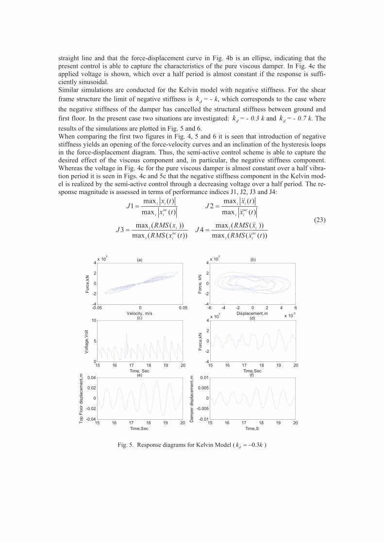
straight line and that the force-displacement curve in Fig. 4b is an ellipse, indicating that the
present control is able to capture the characteristics of the pure viscous damper. In Fig. 4c the
applied voltage is shown, which over a half period is almost constant if the response is suffi-
ciently sinusoidal.
Similar simulations are conducted for the Kelvin model with negative stiffness. For the shear
frame structure the limit of negative stiffness is dk = - k, which corresponds to the case where
the negative stiffness of the damper has cancelled the structural stiffness between ground and
first floor. In the present case two situations are investigated: dk = - 0.3 k and dk = - 0.7 k. The
results of the simulations are plotted in Fig. 5 and 6.
When comparing the first two figures in Fig. 4, 5 and 6 it is seen that introduction of negative
stiffness yields an opening of the force-velocity curves and an inclination of the hysteresis loops
in the force-displacement diagram. Thus, the semi-active control scheme is able to capture the
desired effect of the viscous component and, in particular, the negative stiffness component.
Whereas the voltage in Fig. 4c for the pure viscous damper is almost constant over a half vibra-
tion period it is seen in Figs. 4c and 5c that the negative stiffness component in the Kelvin mod-
el is realized by the semi-active control through a decreasing voltage over a half period. The re-
sponse magnitude is assessed in terms of performance indices J1, J2, J3 and J4:
max ( ) max ( )1 2
max ( ) max ( )
max ( ( )) max ( ( ))3 4
max ( ( ( )) max ( ( ( ))
i i i i
uc uc
i i i i
i i i i
uc uc
i i i i
x t x tJ J
x t x t
RMS x RMS xJ J
RMS x t RMS x t
� �
� �
����
����
(23)
Fig. 5. Response diagrams for Kelvin Model ( 0.3dk k� � )
-0.05 0 0.05-4
-2
0
2
4x 10
7
Velocity, m/s
Forc
e,k
N
(a)
-6 -4 -2 0 2 4 6
x 10-3
-4
-2
0
2
4x 10
7
Displacement,m
Forc
e,
kN
(b)
15 16 17 18 19 200
5
10
Time, Sec
Voltage,V
olt
(c)
15 16 17 18 19 20-4
-2
0
2
4x 10
7
Time,Sec
Forc
e,k
N
(d)
15 16 17 18 19 20-0.04
-0.02
0
0.02
0.04
Time,Sec
Top F
loor
dis
pla
cem
ent,
m (e)
15 16 17 18 19 20-0.01
-0.005
0
0.005
0.01
Time,S
Dam
per
dis
pla
cem
ent,
m
(f)

Fig.6. Response diagrams for Kelvin Model ( 0.7dk k� � )
where superscript uc indicates the undamped case. The values of the J1-J4 are given in Table 2
for the three damper models. It is found that all three damper models introduce a significant re-
sponse reduction compared to the undamped case. The influence of negative stiffness is mod-
erate compared to the viscous case and the increase in negative stiffness from dk = - 0.3 k to dk
= - 0.7 k is without significant impact. It was found that the voltage generated from inverse
damper in some case was quite noisy. Therefore a simple first order filter has been implemented
to improve the signal quality of the voltage (Yang 2001)
fil filu u u. .� �� (24)
where desu is the desired force and u is the actual force generated from inverse MR damper
model. Here � is chosen as 31.4 inspired by Yang (2001).
System Model J1 J2 J3 J4
Pure Viscous 0.6995 0.9526 0.7154 0.6789
Kelvin with negative stiffness ( 0.3dk k� � ) 0.6745 0.9332 0.6909 0.6645
Kelvin with negative stiffness( 0.7dk k� � ) 0.6574 0.9310 0.6799 0.6615
Table2: Performance Analysis
7 CONCLUSION
The semi-active control strategies for MR damper for getting optimal performance for pure
viscous and Kelvin models are investigated above. The optimal force is found for both the cases
from Modal analysis. Then this optimal force is used to get desired voltage for MR damper from
inverse MR damper. The voltage, force, displacement diagrams are compared for both the case
with increasing negative stiffness. From the results it is clearly shown that negative stiffness has
-0.05 0 0.05-4
-2
0
2
4x 10
7
Velocity, m/s
Forc
e,k
N
(a)
-6 -4 -2 0 2 4 6
x 10-3
-4
-2
0
2
4x 10
7
Displacement,m
Forc
e,
kN
(b)
15 16 17 18 19 200
5
10
Time, Sec
Voltage,V
olt
(c)
15 16 17 18 19 20-4
-2
0
2
4x 10
7
Time,Sec
Forc
e,k
N
(d)
15 16 17 18 19 20-0.04
-0.02
0
0.02
0.04
Time,Sec
Top F
loor
dis
pla
cem
ent,
m (e)
15 16 17 18 19 20-0.01
-0.005
0
0.005
0.01
Time,S
Dam
per
dis
pla
cem
ent,
m(f)

significant influence on reduction of displacements and as well as on acceleration. The voltage
requirement is reduced with the increase of negative stiffness. Force-displacement diagram is el-
liptical and changing its inclination angle with the increase of negative stiffness.
For this case earthquake excitation data are used but wind load excitation remains for future
work.
Acknowledgements
This work has been supported by the Danish Agency for Science, Technology and Innovation
via the project 645-06-0371 “Damping of Flexible structures by smart control of semi active de-
vices”.
8 REFERENCE
1. J.R. Høgsberg, S. Krenk, Linear Control strategies for damping of flexible structures,
Journal of Sound and Vibration, Vol. 293 (2006) 59-77
2. G. Yang, B.F. Spencer, H.J. Jung, J.D. Carlson, Dynamic Modeling of large-scale mag-
netorheological damper systems for civil engineering applications, Journal of Engineer-
ing Mechanics, Vol. 130 (2001), No. 9, 1107-1114
3. J.A. Main, S. Krenk, Efficiency and tuning of viscous dampers on discrete systems,
Journal of Sound and Vibration, 286 (2005) 97-122
4. J.R. Høgsberg, S. Krenk, System Reduction and Damping of Flexible Structures, Pro-
ceedings of ECCOMAS Conference on Computational Methods in Structural Dynamics
and Earthquake Engineering, (2007)
5. C.L. Ng, Y.L. Xu, Semi-active control of a building complex with variable friction
dampers, Journal of Engineering Structures,Vol.29 (2007) 1209-1225
6. S.J. Dyke, B.F. Spencer, M.K. Sain, J.D. Carlson, An experimental study of MR dam-
pers for seismic protection, Smart Materials and Structures, Vol. 7(1998) 693-703
7. C.C. Chang, P. Roshke, Neural network modeling of a magneto rheological damper,
Journal of Intelligent Material Systems and Structure, Vol.9 (1999) 755-764
8. L.M. Jansen, S.J. Dyke, Semi-active control strategies for MR dampers: comparative
study, Journal of Engineering Mechanics, ASCE. Vol.126 (1999) 795-803
9. C.C. Chang, T.Y. Yang, Control of Building Using Active Tuned Mass Dampers, Jour-
nal of Engineering Mechanics, Vol.121 N.3 (1995) 355-366�

P5
(Conference paper)
Neural Network modeling of forward and inverse behavior of rotary MR damper
Proceedings of the Twenty Third Nordic Seminar on Computational MechanicsOctober 21–22, Stockholm, Sweden, 2010, 169–172

23rd Nordic Seminar on Computational Mechanics NSCM-23
A. Eriksson and G. Tibert (Eds) © KTH, Stockholm, 2010
NEURAL NETWORK MODELING OF FORWARD AND INVERSE BEHAVIOR OF ROTARY MR DAMPER
NSCM-23
SUBRATA BHOWMIK*,†, JAN HØGSBERG* AND FELIX WEBER†
*Section of Coastal, Maritime and Structural Engineering Department of Mechanical Engineering
Technical University of Denmark Nils Koppels Allé 403, 2800 Lyngby, Denmark E-mail: [email protected], [email protected]
†Structural Engineering Laboratory
Swiss Federal Laboratories for Materials Science and Research (EMPA) Ueberlandstrasse 129, 8600 Duebendorf, Switzerland
Email: [email protected] Key words: Magneto rheological (MR) damper, neural network.
Summary. This paper describes the modeling of a rotary MR damper applying the feed-forward back propagation neural network method. The forward and inverse MR damper behavior are modeled to estimate the force and to solve the force tracking task in real-time. The training and validation data are generated by dynamic tests of the MR damper mounted on a hydraulic testing machine. The training data for the forward model are velocity and current whereby the force is the target. The inverse modeling training data are absolute velocity and absolute force and the current is the target. This new approach is chosen because current is always positive and thereby leads to a small modeling error independently of the sign of velocity. The validation demonstrates that the proposed neural network approach can reliably represent both the forward and inverse dynamic characteristics of the rotary type MR damper.
1 INTRODUCTION
Magneto-rheological (MR) dampers have received considerable attention within the last decades mainly because of their design simplicity, low power requirements, large force range and robustness. Typically, a rotary type MR damper consists of a rotating disk which is enclosed in a rectangular metallic housing filled with the MR fluid. The MR fluid housed within the rotary type MR damper is operated in shear mode. The dissipative torque produced is transformed into a translational force through the crank shaft mechanism. The most common models to describe the dynamic behavior of MR dampers are the Bouc–Wen model [1], the LuGre friction model [2] and the Dahl model [3]. These modeling approaches are fairly complicated due to the high degree of nonlinearities in the system under consideration. From a computational point of view the nonparametric neural network technique is very versatile in connection with most types of nonlinear problems [4].

Subrata Bhowmik, Jan Høgsberg and Felix Weber
2
Therefore, this paper applies this method to model the dynamic behavior of the rotary MR damper.
2 EXPERIMENTAL SET-UP
The experimental test set up and its schematic diagram are shown in Fig. 1. The dSPACE is used to output the desired displacement going to the INSTRON controller, to output the desired current going to the current driver KEPCO and to acquire the measured states such as MR damper force, acceleration of the crank-shaft, actual displacement and current. Sinusoidal and triangular displacements with different frequencies from 0.5 Hz to 2.2 Hz are applied. Triangular displacements are used in order to perform tests at constant damper velocity. Constant and half-sinusoidal currents with different frequencies from 0.5 Hz to 2.2 Hz are also applied. The current of the MR damper under consideration is limited to 4 A and the maximum displacement amplitude is constraint to 10 mm due to the crank-shaft mechanism. The measured data is filtered to remove measurement noise and offsets in order to get the training data for the neural networks.
KEPCO Current Driver
Hydraulic Actuator
MR Damper
Load Cell
Instron PC Unit
dSPACEController Unit
Accelerometer
MR Damper
Actuator
DamperforceLoad Cell
Currentdriver
PowerSupply
DisplacementCommand
dSPACE
Acceleration
ActualDisp
Figure 1. Experimental set-up and its schematic view
3 NEURAL NETWORK MODELING
Feed forward neural network (FFNN) is capable of modeling any nonlinear behaviour with acceptable accuracy. One data set is use as training data and another as validation set.
3.1 Forward MR damper modeling using FFNN
The identification methodology for the modeling of the forward dynamics of MR damper using the FFNN approach is illustrated in Fig. 2. The input states are current and velocity and their associated delay values. The velocity is required due to its significant influence on the hysteretic behavior of the MR damper. It is derived by numerical differentiation of the measured displacement. The noise resulting from the differentiation is removed by additional low pass filtering. The difference between modeled and measured MR damper force, i.e. the
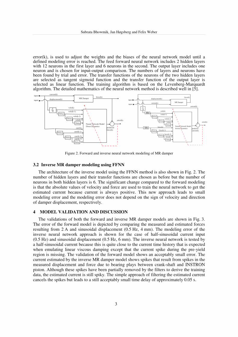
Subrata Bhowmik, Jan Høgsberg and Felix Weber
3
error(k), is used to adjust the weights and the biases of the neural network model until a defined modeling error is reached. The feed forward neural network includes 2 hidden layers with 12 neurons in the first layer and 6 neurons in the second. The output layer includes one neuron and is chosen for input-output comparison. The numbers of layers and neurons have been found by trial and error. The transfer functions of the neurons of the two hidden layers are selected as tangent sigmoid function and the transfer function of the output layer is selected as linear function. The training algorithm is based on the Levenberg-Marquardt algorithm. The detailed mathematics of the neural network method is described well in [5].
MR Damper
current(k)
displacement(k)
force(k)
Neural Network Model
Direct Dynamics
Delay
Delay
Delay
velo(k)
velo(k-1)
velo(k-2)
velo(k-3)
curr(k-1)
curr(k-2)
curr(k-3)
d
dt
+-
error(k)
predicted
force(k)
Delay
Delay
curr(k)
Delay
input
input
MR Damper
displacement(k)
current(k)
force(k)
Neural Network Model
Inverse Dynamics
+-
error(k)
predicted
current(k)
current(k)
Delay
Delay
Delay
velo(k)
velo(k-1)
velo(k-2)
velo(k-3)
d
dt
Delay
Delay
Delay
force(k)
force(k-1)
force(k-2)
force(k-3)
input
input
Abs
Abs
Figure 2. Forward and inverse neural network modeling of MR damper
3.2 Inverse MR damper modeling using FFNN
The architecture of the inverse model using the FFNN method is also shown in Fig. 2. The number of hidden layers and their transfer functions are chosen as before but the number of neurons in both hidden layers is 6. The significant change compared to the forward modeling is that the absolute values of velocity and force are used to train the neural network to get the estimated current because current is always positive. This new approach leads to small modeling error and the modeling error does not depend on the sign of velocity and direction of damper displacement, respectively.
4 MODEL VALIDATION AND DISCUSSION
The validations of both the forward and inverse MR damper models are shown in Fig. 3. The error of the forward model is depicted by comparing the measured and estimated forces resulting from 2 A and sinusoidal displacement (0.5 Hz, 4 mm). The modeling error of the inverse neural network approach is shown for the case of half-sinusoidal current input (0.5 Hz) and sinusoidal displacement (0.5 Hz, 6 mm). The inverse neural network is tested by a half-sinusoidal current because this is quite close to the current time history that is expected when emulating linear viscous damping except that the current spike during the pre-yield region is missing. The validation of the forward model shows an acceptably small error. The current estimated by the inverse MR damper model shows spikes that result from spikes in the measured displacement and force due to bearing plays between crank-shaft and INSTRON piston. Although these spikes have been partially removed by the filters to derive the training data, the estimated current is still spiky. The simple approach of filtering the estimated current cancels the spikes but leads to a still acceptably small time delay of approximately 0.05 s.

Subrata Bhowmik, Jan Høgsberg and Felix Weber
4
5 CONCLUSIONS
This investigation employed the back propagation feed forward neural network method to model the forward and inverse dynamics of an MR damper. The training data was taken on a prototype rotary MR damper that was connected to a hydraulic machine imposing sinusoidal and triangular displacements and constant and half sinusoidal current time histories. The goal of the forward MR damper model was to capture accurately the behavior of the MR damper behavior whereas the inverse MR damper model will later be used for the control force tracking when the MR damper will be connected to a shear frame. The novelty in the proposed neural network when modeling the inverse MR damper behavior is that the absolute values of velocity and force are used to estimate the damper current since current is always positive. The validations of both the forward and inverse MR damper models show that the applied neural network approaches capture the main MR damper dynamics with acceptable accuracy. However, the preliminary results demonstrate that the modeling accuracies can still be improved by further optimization of the filters that are used to process the measurement data to derive the training data for the neural network training.
48.5 49 49.5 50
0
0.5
1
1.5
2
2.5
3
3.5
4
4.5
Time, S
Cur
rent
, A
desired current predicted current predicted current−filtered
Figure 3. Validation of forward and inverse neural network models
REFERENCES
[1] T. Tse, C. Chang, Shear-Mode Rotary Magnetorheological Damper for Small-Scale Structural Control Experiments, Journal of Structural Engineering, 130 (2004) 904-910.
[2] C. Boston, F. Weber, L.Guzzella, Modeling of a disc-type magnetorheological damper, Smart Mater. and Struct., 19 (2010) 045005 (12pp).
[3] F. Ikhouane, S. Dyke, Modeling and identification of a shear mode magneto rheological damper, Smart Mater. and Struct., 16 (2007) 605-616.
[4] H. Metered, P. Bonello, S. Oyadiji, The experimental identification of magnetorheological dampers and evaluation of their controllers, Mechanical Systems and signal Processing, 24 (2010) 976-994.
[5] C. Chang, L. Zhou, Neural Network Emulation of Inverse Dynamics for a Magneto rheological Damper, Journal of Structural Engineering, 128 (2002) 231-239.


DTU Mechanical Engineering
Section of Coastal, Maritime and Structural Engineering
Technical University of Denmark
Nils Koppels Allé, Bld. 403
DK-2800 Kgs. Lyngby
Denmark
Phone (+45) 4525 1360
Fax (+45) 4588 4325
www.mek.dtu.dk
ISBN: 978-87-90416-70-6
DCAMM
Danish Center for Applied Mathematics and
Mechanics
Nils Koppels Allé, Bld. 404
DK-2800 Kgs. Lyngby
Denmark
Phone (+45) 4525 4250
Fax (+45) 4593 1475
www.dcamm.dk
ISSN: 0903-1685