P R IMA R Y R E S E A R CH A R T I C L E

Modelled biophysical impacts of conservation agriculture onlocal climates

Annette L. Hirsch1 | Reinhard Prestele2 | Edouard L. Davin1 |

Sonia I. Seneviratne1 | Wim Thiery1,3 | Peter H. Verburg2,4

1Institute for Atmospheric and Climate

Science, ETH Zurich, Zurich, Switzerland

2Environmental Geography Group, Institute

for Environmental Studies, Vrije Universiteit

Amsterdam, Amsterdam, The Netherlands

3Department of Hydrology and Hydraulic

Engineering, Vrije Universiteit Brussel,

Brussels, Belgium

4Swiss Federal Research Institute WSL,

Birmensdorf, Switzerland

Correspondence

Annette L. Hirsch, Institute for Atmospheric

and Climate Science, ETH Zurich, 8092

Zurich, Switzerland.

Email: annette.hirsch@env.ethz.ch

Funding information

Eidgenössische Technische Hochschule

Zürich, Grant/Award Number: Fel‐45 15‐1;FP7 Ideas: European Research Council,

Grant/Award Number: 603542, FP7‐IDEAS‐ERC‐311819, FP7‐IDEAS‐ERC‐617518

Abstract

Including the parameterization of land management practices into Earth System

Models has been shown to influence the simulation of regional climates, particularly

for temperature extremes. However, recent model development has focused on

implementing irrigation where other land management practices such as conserva-

tion agriculture (CA) has been limited due to the lack of global spatially explicit data-

sets describing where this form of management is practiced. Here, we implement a

representation of CA into the Community Earth System Model and show that the

quality of simulated surface energy fluxes improves when including more informa-

tion on how agricultural land is managed. We also compare the climate response at

the subgrid scale where CA is applied. We find that CA generally contributes to

local cooling (~1°C) of hot temperature extremes in mid‐latitude regions where it is

practiced, while over tropical locations CA contributes to local warming (~1°C) due

to changes in evapotranspiration dominating the effects of enhanced surface albedo.

In particular, changes in the partitioning of evapotranspiration between soil evapora-

tion and transpiration are critical for the sign of the temperature change: a cooling

occurs only when the soil moisture retention and associated enhanced transpiration

is sufficient to offset the warming from reduced soil evaporation. Finally, we exam-

ine the climate change mitigation potential of CA by comparing a simulation with

present‐day CA extent to a simulation where CA is expanded to all suitable crop

areas. Here, our results indicate that while the local temperature response to CA is

considerable cooling (>2°C), the grid‐scale changes in climate are counteractive due

to negative atmospheric feedbacks. Overall, our results underline that CA has a non-

negligible impact on the local climate and that it should therefore be considered in

future climate projections.

K E YWORD S

CESM, climate‐effective land management, CLM, land‐based mitigation, subgrid‐scaleinfluences, temperature extremes, tillage

- - - - - - - - - - - - - - - - - - - - - - - - - - - - - - - - - - - - - - - - - - - - - - - - - - - - - - - - - - - - - - - - - - - - - - - - - - - - - - - - - - - - - - - - - - - - - - - - - - - - - - - - - - - - - - - - - - - - - - - - - - - - - - - - - - - - - - - - - - - - - - - - - - - - - - - - - - - - - - - - - - - - - -This is an open access article under the terms of the Creative Commons Attribution License, which permits use, distribution and reproduction in any medium,

provided the original work is properly cited.

© 2018 The Authors. Global Change Biology Published by John Wiley & Sons Ltd.

Received: 6 October 2017 | Accepted: 1 June 2018

DOI: 10.1111/gcb.14362

Glob Change Biol. 2018;1–17. wileyonlinelibrary.com/journal/gcb | 1

1 | INTRODUCTION

Agricultural land management has a substantial impact on regional

climate (e.g. Davin, Seneviratne, Ciais, Olioso, & Wang, 2014; Hirsch,

Wilhelm, Davin, Thiery, & Seneviratne, 2017; Luyssaert et al., 2014;

Thiery et al., 2017), and influences local responses to projected cli-

mate change (Hirsch et al., 2017). However, historically climate

model simulations contributing to the various Coupled Model Inter-

comparison Projects (CMIPs) have had limited or no representation

of agricultural land management. Recently, considerable progress has

been made to move away from basic representations of agricultural

activity in Earth System Models (ESMs) where crops are typically

modelled with the same physiological characteristics as C3 grasses.

This includes the parameterization of irrigation (e.g. Cook, Shukla,

Puma, & Nazarenko, 2014; De Vrese, Hagemann, & Claussen, 2016;

Decker, Ma, & Pitman, 2017; Guimberteau, Laval, Perrier, & Polcher,

2012; Harding & Snyder, 2012; Lawston, Santanello, Zaitchik, &

Rodell, 2015; Qian, Huang, Yang, & Berg, 2013; Sacks, Cook, Buen-

ning, Levis, & Helkowski, 2008; Thiery et al., 2017) to fully interac-

tive crop modules that incorporate different crop varieties with

defined growing seasons and fallow periods (e.g. Levis et al., 2012).

However, conservation agriculture, involving minimal or no til-

lage, crop residue management and crop rotation (Kassam, Friedrich,

Derpsch, & Kienzle, 2015), is generally not considered in the land

surface component of ESMs. This is due to (a) a lack of global data-

sets characterizing where conservation agriculture is practiced and

(b) the high uncertainty in soil carbon sequestration under minimal

tillage regimes (Neufeldt, Kissinger, & Alcamo, 2015; Powlson et al.,

2014). Nevertheless, the adoption of these land management prac-

tices is seen as a potential climate mitigation and adaptation strategy

that also has climate impacts beyond its impact on carbon sequestra-

tion (Davin et al., 2014; Lobell, Bala, & Duffy, 2006). Here, we take

the first step towards resolving the representation of conservation

agriculture within ESMs by implementing a simple parameterization

within a state‐of‐the‐art ESM using a new spatially explicit dataset

on conservation agriculture as input (Prestele, Hirsch, Davin, Senevi-

ratne, & Verburg, 2018).

The adoption of conservation agriculture has increased from

45 Mha in 1999 to 157 Mha in 2013 (Derpsch, Friedrich, Kassam, &

Hongwen, 2010; Kassam et al., 2015). This increase is partly associ-

ated with the need to increase productivity in response to various

external economic and environmental pressures (Kassam et al.,

2015). Furthermore, this increase is influenced by the growing

awareness of how traditional tillage‐based production systems have

a negative impact on soil quality by increasing soil erosion rates and

changing biogeochemical cycling due to soil disturbance (Govers,

Quine, Desmet, & Walling, 1996; Govers, Vandaele, Desmet, Poesen,

& Bunte, 1994; Quinton, Govers, Van Oost, & Bardgett, 2010; Van

Oost et al., 2007; Wang et al., 2017) which has potential negative

consequences for yield. In particular, yield levels with minimal tillage

are comparable or even higher than conventional tillage systems

(Kassam et al., 2015). Nonetheless, a recent meta‐analysis does iden-

tify that yield gains from minimal tillage are mostly possible when

combined with both crop residue management and crop rotation,

particularly for drier climates rather than humid climates (Pittelkow

et al., 2015). There are, however, some critical limitations on where

conservation agriculture is possible. This includes practical knowl-

edge about conservation agriculture and investment costs—including

time and machinery—to establish and maintain the soil mulch, and

finally the political and social support to move away from traditional

farming practices (Kassam et al., 2015). Furthermore, conservation

agriculture has biophysical feedbacks on climate associated with how

the presence of a crop residue alters the surface energy balance

through changes in surface albedo, roughness, and evapotranspira-

tion (Davin et al., 2014).

The examination of the potential impacts of no‐till farming, an

essential part of conservation agriculture, on the climate system has

been done in climate models. However, existing studies often use an

idealized approach to evaluate the climate implications of a full con-

version of global croplands (e.g. Davin et al., 2014; Hirsch et al.,

2017; Lobell et al., 2006; Wilhelm, Davin, & Seneviratne, 2015). For

example, Lobell et al. (2006) compare the impact of four different

land management practices on present‐day climate. In that study,

no‐till farming was represented by multiplying the soil albedo by 1.5

over the fractional area designated as croplands in the model. The

results demonstrated the potential of increasing surface albedo to

cool surface temperatures by reducing the available energy at the

surface. Davin et al. (2014) apply more conservative changes over

Europe in a regional climate model by increasing surface albedo over

croplands by 0.1 and increasing the soil resistance by a factor of 4

to represent the effects of crop residue on evaporation. They found

that the cooling potential of no‐till farming was greater for tempera-

ture extremes than mean temperature. Wilhelm et al. (2015) also

take an idealized approach to represent no‐till via albedo changes

and demonstrate that the temperature response scales linearly with

the magnitude of the albedo change, the spatial extent, and the tem-

poral extent. This was confirmed in Hirsch et al. (2017) who also

demonstrate that the cooling potential from increased surface albedo

associated with no tillage is comparable to that of irrigation, and

therefore the effects of surface albedo changes associated with agri-

cultural practices are important. Although these studies (i.e. Davin et

al., 2014; Hirsch et al., 2017; Lobell et al., 2006; Wilhelm et al.,

2015) use an idealized approach to examine the cooling potential of

various land management practices, they all demonstrate that

changes in albedo and evapotranspiration associated with no‐tillfarming have implications for climate, particularly temperature

extremes, and that therefore investment in further developing

parameterizations to represent this land management practice, and

more specifically conservation agriculture, within ESMs is worth pur-

suing.

In this study, we build upon previous research with ESMs to

examine the climate implications of agricultural land management.

Deviating from the idealized approach used in previous studies, we

use a new global conservation agriculture dataset (Prestele et al.,

2018) to constrain the application of albedo and evapotranspiration

changes towards a more realistic distribution of this land

2 | HIRSCH ET AL.

management practice. We also limit albedo changes to the soil sur-

face rather than the canopy albedo as in Wilhelm et al. (2015) and

Hirsch et al. (2017) to emulate how the presence of crop residues

alters the background surface albedo. Furthermore, we model this

albedo change as a function of soil colour, recognizing that the

albedo change from crop residue will be smaller over brighter soils

than darker soils. We also aim to assess whether applying a more

conservative approach of the biophysical effects of conservation

agriculture within an ESM can improve the simulation of present‐dayclimate and we explore the possible climate sensitivity to different

conservation agriculture estimates.

2 | MATERIALS AND METHODS

2.1 | Model description and setup

We use the Community Earth System Model (CESM) version 1.2

(Hurrell, Holland, & Gent, 2013) with prescribed sea surface temper-

atures (SSTs) and sea ice fraction using a setup that closely follows

the framework of the Atmospheric Model Intercomparison Project

(AMIP). For all simulations we use the F1850PDC5 component set

for the present‐day period commencing from 1976 to 2010. This

includes using the Community Atmosphere Model version 5 (Neale

et al., 2012) with transient greenhouse gas concentrations prescribed

from measurements and the Community Land Model (CLM) version

4 (Oleson, Lawrence, & Bonan, 2010) with prescribed vegetation

phenology derived from MODIS (Lawrence & Chase, 2007). The land

surface heterogeneity is represented at the subgrid scale by defining

multiple land units consisting of different surface types (e.g. vege-

tated, urban, wetland, lake, and glacier). The vegetated land unit

includes 16 plant functional types (PFT) with the global distribution

set to the year 2000 based on MODIS data and on Ramankutty,

Evan, Monfreda, and Foley (2008) for croplands (Lawrence & Chase,

2007).

We use the same set of control simulations as those evaluated

in Thiery et al. (2017). This consists of a 5‐member control ensemble

with a horizontal resolution of 0.9° latitude × 1.25° longitude, start-

ing from 1976 to 2010 (35 years), where the first 5 years are dis-

carded as spin‐up. Ensemble members are generated by applying a

random perturbation of 10−14 to the atmospheric temperature initial

conditions (Fischer, Beyerle, & Knutti, 2013). We prescribe SSTs and

sea ice to focus on the influence of land–atmosphere interactions

without the added complexity of ocean–atmosphere feedbacks on

the climate system. In addition to the control ensemble, we run four

5‐member ensemble experiments corresponding to the four different

conservation agriculture estimates described in the following section:

BASE, LOW, HIGH, and POT.

2.2 | Description of conservation agriculturedataset

We use the conservation agriculture dataset developed by Prestele

et al. (2018) to prescribe the spatial distribution of conservation

agriculture in the CESM simulations. This dataset builds on the

national‐level estimates of conservation agriculture published in Kas-

sam et al. (2015) and additional regional datasets. The aggregated

estimates of conservation agriculture were downscaled to a 5‐arc‐minute regular grid using GIS‐based multi‐criteria analysis. The

downscaling algorithm considers several spatial determinants of con-

servation agriculture adoption, including biophysical (aridity and soil

degradation) and socio‐economic (farm size, access to suitable equip-

ment, and poverty level) variables. Uncertainties due to inconsisten-

cies in the definition of conservation agriculture (e.g. Carmona et al.,

2015; Hobbs, 2007) and the lack of systematic reporting schemes

(Kassam et al., 2015) are represented by a range of spatially explicit

maps (BASE, LOW, and HIGH). In particular, the baseline estimate

(BASE) represents the most likely distribution of conservation agri-

culture based on the available data sources with a global area of

158 Mha. The uncertainty range in the LOW and HIGH estimates

was derived from alternative country‐level datasets on tillage prac-

tices not used in the BASE estimate. Alternative data could be

obtained for approximately 30% of the global arable land area. For

the remaining area a default uncertainty range of ±25% was added

to the national level CA areas of the BASE estimate. Globally, this

resulted in 122 and 215 Mha of conservation agriculture for the

LOW and HIGH estimates, respectively. To identify the global future

potential for conservation agriculture, Prestele et al. (2018) also pro-

vide a POTential estimate. This estimate assumes that all agricultural

land that is generally suitable for management under the principles

of conservation agriculture is converted in the future (1130 Mha

globally). This estimate still deviates strongly from earlier idealized

implementations of conservation agriculture on all arable land

because there are many conditions that constrain the adoption of

conservation agriculture. For methodological details and additional

information on the different estimates we refer to Prestele et al.

(2018).

2.3 | Implementation of conservation agriculture

We implement conservation agriculture (CA) into CESM by splitting

the existing CLM crop PFT into a fraction under conservation agri-

culture (CCA) and a fraction under conventional management (CCM).

Therefore, both forms of management are possible within a grid cell.

The fractions of cropland under conservation agriculture and under

conventional management are determined as follows:

CCA ¼ CALL � ACA

ACROP

� �(1)

CCM ¼ CALL � 1� ACA

ACROP

� �(2)

where CALL is the default CLM crop fraction, ACA is the area under

conservation agriculture, and ACROP is the total cropland area. Both

ACA and ACROP are obtained from the CA dataset (see previous sec-

tion) and are conservatively aggregated from the original 5‐arc‐min-

ute resolution to the CLM resolution used in this study (0.9°

HIRSCH ET AL. | 3

latitude × 1.25° longitude). By using this approach we avoid poten-

tial grid conflicts, as the CA dataset is based on the HYDE cropland

extent for the year 2012, whereas the CLM land cover uses 2000

cropland extents from Ramankutty et al. (2008). The distribution of

the CA crop PFT for the four CA estimates is illustrated in Figure 1.

Surface albedo (α) in CLM is calculated at the subgrid level for

canopy and soil surfaces separately, which are then aggregated to a

total surface albedo as a weighted combination of snow‐free and

snow‐covered albedos. All albedo terms are modelled using a two‐stream approximation for radiative transfer to determine the direct

and diffuse radiation contributions. To reflect the higher surface

albedo of crop residue, we increase the soil albedo for the CA crop

PFT using the following function:

Δαsoils;s ¼ min 0:1;0:1

NS þ 1� s

� �(3)

where NS is the number of soil classes (here we use 20) and s is the

soil colour index (1–20 with 1 the brightest and 20 the darkest soil).

We limit the maximum change in soil albedo to 0.1, which is consid-

ered the maximum possible change in surface albedo by crop residue

(Davin et al., 2014; Hirsch et al., 2017). Therefore, we constrain the

albedo change by the soil colour, recognizing that the effective

albedo change will be minimal on brighter soils compared to darker

soils with the albedo change ranging from 0.005 for the brightest

soil to 0.100 for the darkest soil. We assume that the crop residue is

present all year, but our implementation ensures that the effect of

the increased soil albedo on the total surface albedo is dampened

during the growing season by the presence of canopy cover.

The presence of crop residue also has an impact on the amount

of soil evaporation. Therefore, to reduce the soil evaporation, and

mimic the effect of a crop residue layer for no tillage areas, we

double the litter resistance of the soil column corresponding to the

CA crop PFT. Note that the litter resistance is added to the aero-

dynamic resistance which together limit water vapour transfer from

the ground to the atmosphere by scaling the soil latent heat flux.

Various perturbations of the litter resistance were tested in offline

land surface only simulations. We chose to double the litter resis-

tance term so that the change in soil moisture was limited to

within 10%–20%, which is consistent with observational evidence

of the effect of crop residue compared to tilled soils (De Vita, Di

Paolo, Fecondo, Di Fonzo, & Pisante, 2007). Furthermore, we note

that the CA and conventionally managed crop PFTs have been put

on separate soil columns to account for the fact that the presence

of a crop residue will influence the available soil moisture of the

CA crop PFT.

Due to a lack of global datasets that characterize tillage intensity,

we do not implement partial residue cover. Furthermore, we do not

modify the surface roughness or infiltration rates due to limitations

in how these vary according to residue thickness. We restrict our

implementation to changing the biophysical properties of the CA

crop, but recognize that the presence of crop residues and absence

of soil disturbance do influence the carbon stores in litter and the

upper soil layers.

2.4 | Evaluation datasets

We evaluate the performance of all experiments by comparing the

model output to several observational datasets. For surface albedo we

use the monthly European Space Agency Global Albedo product ver-

sion D17 over 1998–2010 (GlobAlbedo; Danne, Zuehlke, & Krämer,

2011). For 2 m air temperature and precipitation we use the monthly

(d) POT

(b) LOW

(c) HIGH

(a) BASE

Fraction of Grid Cells with CA [%]

F IGURE 1 Conservation agriculture extents mapped to CLM cropPFT for the four different estimates: (a) BASE, (b) LOW, (c) HIGH,and (d) POT. The red boxes in (a) denote the regional domainsexamined in greater detail including Western North America (WNA),Central North America (CNA), South‐eastern South America (SSA),Central Europe (CEU), Mediterranean (MED), and Southern Australia(SAU)

4 | HIRSCH ET AL.

Climate Research Unit version 3.22 dataset (CRU; Harris, Jones,

Osborn, & Lister, 2014). We also use the monthly Global Precipitation

Climatology Project version 2.2 dataset (GPCP; Huffman et al., 2001).

Surface shortwave and longwave radiation is compared to the satel-

lite‐based monthly Global Energy and Water Cycle Exchanges

(GEWEX) Project Surface Radiation Budget version REL3 over 1984–2007 (SRB; Stackhouse et al., 2011). For the sensible and latent heat

fluxes, we use data from the monthly Fluxnet Model Tree Ensembles

dataset over 1982–2010 (MTE; Jung et al., 2010), the monthly bench-

mark synthesis for diagnostic evapotranspiration over 1989–2005(LandFlux‐EVAL; Mueller et al., 2013), and the daily Global Land Eva-

poration Amsterdam Model version 3a (GLEAM; Miralles et al., 2011).

Finally, we evaluate temperature extremes using the monthly Global

Historical Climatology Network (GHCNDEX; Donat et al., 2013a) and

version 2 of the monthly Hadley Centre Extremes dataset (HadEX2;

Donat et al., 2013b). We conduct the model evaluation over 1981–2010 or otherwise limited to the period of data availability noted

above. All observational products are regridded to the CESM resolu-

tion using conservative remapping.

2.5 | Analysis

Our analysis uses the ensemble average daily output from CESM to

examine changes in the extremes indices as defined by the Expert

Team on Climate Change Detection and Indices (ETCCDI, Zhang et

al., 2011). In this study we present the impact of CA on the follow-

ing two extremes indices: the annual maximum daytime temperature

(TXx) and the annual minimum night‐time temperature (TNn). Other

ETCCDI extremes indices including the number of consecutive dry

days and extreme precipitation indices did not show systematic

responses to the modifications we applied in CESM and are there-

fore omitted.

As CESM can provide output at the PFT level we are able to

examine how the distinction between the CA and CM crops influ-

ences the subgrid‐scale climate. Furthermore, we can also compare

this to the standard grid‐scale surface variables (e.g. 2‐m air tempera-

ture, latent heat flux, etc.) that are calculated as a weighted combi-

nation of the fractional contributions from each of the PFTs. To

evaluate the impact of CA on the grid‐scale surface climate we com-

pute the mean difference between the experiment and the control

using the ensemble mean monthly time series. We scale this mean

difference by the standard deviation, to account for the internal vari-

ability in CESM such that differences that exceed the standard devi-

ation are a real signal and not part of the noise. To examine the

impact of CA at the subgrid‐scale surface climate we compute the

mean difference between the CA and CM PFT‐level output, also

scaled by the standard deviation to enable comparison to the grid‐scale surface climate response.

To examine changes in surface temperature (TS) in response to

conservation agriculture, we use the surface energy balance decom-

position method applied in previous studies (e.g. Akkermans, Thiery,

& Van Lipzig, 2014; Hirsch et al., 2017; Luyssaert et al., 2014; Thiery

et al., 2015, 2017). Here, we express the surface energy balance as:

ɛσT4S ¼ ð1� αÞSWi þ LWi � LHF� SHF� R (4)

where ε is the surface emissivity, σ is the Stefan‐Boltzmann constant

(5.67 × 10−8 W m−2 K−4), α is the surface albedo, SWi is the incom-

ing shortwave radiation, and LWi is the incoming longwave radiation,

LHF is the latent heat flux and SHF is the sensible heat flux. The

residual term (R) includes the ground heat flux and changes in sub-

surface heat storage. The change between the experiment and con-

trol (denoted as Δ) is calculated by taking the derivative of

Equation 4 with respect to TS and solving for ΔTS:

ΔTS ¼ 1

4ɛσT3S;CTL

�� SWiΔαþ ð1� αÞΔSWi

þ ΔLWi � ΔLHF� ΔSHF� ΔR� : (5)

To examine regional changes we focus our analysis over

regions where conservation agriculture is extensive. We use the

regions defined in the IPCC Special Report on Managing the Risks

of Extreme Events (SREX) (IPCC, 2012; Seneviratne et al., 2012).

Of these SREX regions, we present the results for: Western North

America (WNA), Central North America (CNA), South‐easternSouth America (SSA), Central Europe (CEU), Mediterranean (MED),

and Southern Australia (SAU). These regions are illustrated in

Figure 1a.

3 | RESULTS

3.1 | Sensitivity of model skill to the inclusion ofCA

In this section, we focus on how the existing CESM climate simula-

tion skill (i.e. how well the simulations agree with the observations)

is changed by including the biophysical effects of CA from the

BASE experiment relative to the skill obtained in the control simu-

lation without CA (CTL). This includes examining the change in the

bias for the present‐day climatology and root mean square error

(RMSE) for key variables, such as the surface albedo, net shortwave

(SWnet) and longwave (LWnet) radiation, the latent heat flux (LHF),

and 2 m air temperature (T2M) (Figure 2). While the bias in the

surface albedo generally increases in the BASE experiment relative

to the CTL for locations where CA is applied, this increase is very

small (Figure 2a). The corresponding response in the radiation bal-

ance indicates a general decrease in the bias over large areas, par-

ticularly over Asia and North America, for SWnet (Figure 2c), LWnet

(Figure 2e), and T2M (Figure 2i). For South America, there is an

increase in the SWnet bias (~1 W/m2), but a decrease in the LHF

bias (Figures 2c,g). Note that these changes in bias extend beyond

the regions where CA is applied and, therefore, despite changes in

the bias indicating some improvement in the simulation skill this

result may still be influenced by the internal variability in the

model. Similarly, the percent change in RMSE indicates that there

is some skill improvement in simulating the temporal variability,

particularly for the northern mid‐latitude regions with a 5%–10%error reduction for the surface albedo, SWnet, LWnet, LHF, and

HIRSCH ET AL. | 5

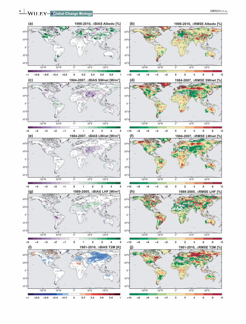
(b) 1998-2010, RMSE Albedo [%] 1998-2010, BIAS Albedo [%] (a)

(d) 1984-2007, RMSE SWnet [%] 1984-2007, BIAS SWnet [W/m2] (c)

(f) 1984-2007, RMSE LWnet [%] 1984-2007, BIAS LWnet [W/m2] (e)

(h) 1989-2005, RMSE LHF [%] 1989-2005, BIAS LHF [W/m2] (g)

(j) 1981-2010, RMSE T2M [%] 1981-2010, BIAS T2M [K] (i)

6 | HIRSCH ET AL.

T2M (Figure 2b,d,f,h,j). However, at higher latitudes (50N‐90N)

there is a decrease in skill with a 6%–10% increase in RMSE. Simu-

lation skill over South‐eastern South America (SSA) also improves

for T2M with a 10% reduction in error, despite some decrease in

skill for LHF. Generally, Figure 2 demonstrates that there is

improvement in simulation skill, but that this is not uniform across

the global domain.

As we are interested in how the uncertainty between the dif-

ferent CA estimates influences simulation skill, we examine the

added value of including CA for different climate variables over

the regions where the CA extent is greatest (Figure 3). We evalu-

ate the added value by calculating for each region the change (ex-

periment minus control) in the spatiotemporal root mean square

error. Accounting for CA generally improves the simulation skill

over the Mediterranean for all variables and CA estimates. For

other regions, including WNA, CNA, and CEU, we find enhanced

skill for some variables. For SSA and SAU, the added value is lim-

ited for all CA estimates. The BASE (Figure 3a) and LOW (Fig-

ure 3b) CA estimates contribute the most to improved simulation

skill, likely due to the more realistic distribution of CA in these

cases. Finally, if we consider the grid cells where land fraction

within CESM exceeds 50% (“all land”) or just the grid cells that

have a nonzero CA fraction (“CA Land”) is present, there is added

value for most variables over the grid cells where CA has been

applied, particularly for the LOW estimate. Note that for precipita-

tion the added value is sensitive to which observational precipita-

tion product is used and is likely a result of the considerable

uncertainty between these datasets (e.g. Adler, Kidd, Petty, Moris-

sey, & Goodman, 2001). Therefore, we are confident that our

implementation of the biophysical effects of CA on the regional‐scale climate has added value.

3.2 | Effect of conservation agriculture on climate

Using the PFT‐level outputs from CLM it is possible to examine the

subgrid‐scale differences between the CA and conventionally man-

aged (CM) crops (Figure 4). This subgrid‐scale effect (CA minus

CM), representing the local effect of CA, can be compared to the

“grid scale” effect computed by comparing the BASE and CTL sim-

ulations. To remove the internal climate variability from the signal

we normalize the mean difference, either BASE minus CTL for grid

scale or CA minus CM for subgrid scale, by the standard deviation.

Generally, at the grid scale, changes in SWnet, LHF, SHF, and Ts are

small (Figure 4, left column), suggesting that the model response is

dampened by internal climate variability. However, the subgrid‐scaleresponse (Figure 4, right column), which shows the difference

F IGURE 2 Contour maps illustrating skill changes from the implementation of conservation agriculture: (a, c, e, g, and i) change in theclimatological model bias (model minus observations) between BASE and CTL and (b, d, f, h, and j) percentage change in the temporal rootmean square error between BASE and CTL. Computed using the monthly time series of the ensemble means. Displayed variables are (a, b)surface albedo, (c, d) net shortwave radiation (SWnet), (e, f) net longwave radiation (LWnet), (g, h) latent heat flux (LHF LandFlux), and (i, j) 2 mair temperature (T2M)

(b) (a) (c)

F IGURE 3 Added value of including conservation agriculture. Percentage change in the spatiotemporal root‐mean‐square error (RMSE) for(a) BASE, (b) LOW, and (c) HIGH relative to the CTL ensemble over different regions (x‐axis) and with respect to 12 observational products (y‐axis). Considered regions are the six SREX regions denoted in Figure 1 plus global land and global CA land. Observational products are foralbedo (GlobAlbedo), latent heat flux LHF (LandFlux‐EVAL, GLEAM), surface net shortwave SWnet and longwave LWnet radiation (SRB), near‐surface air temperature Tmean (CRU), precipitation (CRU and GPCP), monthly maximum daytime temperature TXx (GHCNDEX and HadEX2),and monthly minimum night‐time temperature TNn (GHCNDEX and HadEX2). The RMSEs are computed for the ensemble monthly mean timeseries in every pixel, and subsequently averaged over the selected region. Regions with an observational coverage below 50% are marked inwhite

HIRSCH ET AL. | 7

between the CA and CM crops for the BASE estimate, is substan-

tially larger and often exceeds the internal climate variability of

CESM.

In particular, the subgrid‐scale responses provide insight into

how CA influences the local‐scale climate. More specifically,

decreases in SWnet (Figure 4b) are consistent with the increase in

(a) Grid-scale, SWnet (b) Subgrid-scale, SWnet

(c) Grid-scale, LHF (d) Subgrid-scale, LHF

(e) Grid-scale, SHF (f) Subgrid-scale, SHF

(g) Grid-scale, TS (h) Subgrid-scale, TS

F IGURE 4 Grid‐scale (BASE minus CTL) (a, c, e, and g) and subgrid‐scale (CA(BASE) minus CM(BASE)) (b, d, f, and h) response toimplementation of conservation agriculture calculated as the mean difference normalized by the standard deviation of the differences to filterout the effects of internal variability. Calculated using the monthly mean time series of all ensemble members. For (a, b) net shortwaveradiation (SWnet), (c, d) latent heat flux (LHF), (e, f) sensible heat flux (SHF), and (g, h) near‐surface temperature (TS). Values exceeding 1indicate that the response exceeds the internal climate variability of CESM. Note the different colour axis limits between the grid‐scale andsubgrid‐scale panels

8 | HIRSCH ET AL.

background albedo and tend to be related to the CA fraction with

larger decreases in North and South America. The decrease in

energy absorbed at the surface contributes to the decrease in LHF

(Figure 4d), which is further amplified by the increased resistance to

soil evaporation due to the presence of the crop residue. Again this

response is larger over regions where the CA fraction is greater. The

SHF response is not always consistent with the decrease in SWnet,

with some increases over Eastern North America and South‐easternSouth America. However, this is likely due to the change in the par-

titioning between LHF and SHF arising from the increased resistance

to soil evaporation. These changes in SHF explain why some regions

result in warming of Ts (Figure 4h) rather than cooling as may be

expected by reducing the amount of shortwave energy absorbed by

the surface.

At the subgrid scale, the presence of the crop residue also influ-

ences the partitioning of the LHF between plant transpiration (Fig-

ure 5a) and soil evaporation (Figure 5b). Coincidently, the warming

from CA (e.g. Figure 4h for Ts) often occurs when the decrease in

soil evaporation exceeds the increase in canopy transpiration (e.g.

South America and Eastern North America; Figure 5). Cooling occurs

when the decreased soil evaporation is comparable to the increase

in transpiration. Increases in transpiration arise from more moisture

availability due to less soil evaporation, and therefore, the thickness

of the crop residue is likely to have some influence modulating local

temperatures.

Note that similar responses were found for the LOW and HIGH

CA estimates for the climate variables presented in Figures 4 and 5

with the exception of POT where the application of CA is much

greater and therefore, the corresponding subgrid‐scale changes

between the CA and CM crops were larger over Europe and Asia.

In the literature possible cooling of hot temperature extremes

has been found for regions where tillage is limited (e.g. Davin et al.,

2014). Therefore, we examine the subgrid‐scale changes in both the

annual maximum daytime 2 m air temperature (TXx) and the annual

minimum night‐time temperature (TNn) for each of the CA estimates

(Figure 6). Generally, CA induces cooling of TXx by more than 1°C

for most regions where CA is applied for all estimates (Figure 6, left

column). Interestingly, TXx increases by 1°C over Amazonia in South

America where CA is not practiced. In contrast, CA leads to warming

of TNn consistently of 1°C or more, with the greatest warming

occurring in the locations where CA fraction is greatest in the South-

ern Hemisphere: South‐eastern South America, South Africa and

Southern Australia. Note that the response to TNn is larger in mag-

nitude than the response in TXx. This is likely due to how we param-

eterize CA, where the leaf area index (LAI) modulates how much of

the soil surface is exposed. A larger LAI would therefore lead to a

smaller contrast between the CA and CM crops, which coincides

with TXx during the summer season. The subgrid‐scale response of

TXx and TNn is also remarkably similar between the BASE, LOW,

and HIGH CA estimates (Figure 6a–f), indicating that the sensitivity

of CESM to these different CA estimates is low at this resolution.

3.3 | Effect of conservation agriculture on thesurface energy balance

The response of both the grid‐scale and subgrid‐scale climate to the

implementation of CA in CESM indicates that there are two main

competing effects that influence the surface temperature response.

This includes (a) changes in the surface albedo, which alters how

much energy is available to be partitioned between the sensible and

latent heat fluxes, and (b) changes in the surface resistance which

influences the partitioning between these fluxes. Therefore, an

examination of the change in surface temperature due to the surface

energy balance response is warranted at both global (Figure 7) and

regional (Figure 8) scales.

At the global scale the net effect of CA on all global land grid

cells is a cooling (within 0.1°C) which is largely attributed to

decreases in incoming radiation (SWi and LWi) and enhanced residual

heat storage (Figure 7a) despite changes in SHF contributing to

warming. If one considers the CA grid cells only, then the net effect

on surface temperature is still cooling (within 0.1°C, Figure 7b, note

different axis limits). However in this case, this is largely attributed

to the change in surface albedo, which is larger than the changes in

LHF that lead to warming. Finally, at the subgrid scale (Figure 7c) it

is the albedo and LHF changes that dominate the temperature

response, with the influence of the SHF contributing to a slight

increase in surface temperature. The contrast between Figure 7a

and Figures 7b and 7c indicates that the introduction of CA may

(b) QS

(a) QTR

F IGURE 5 Subgrid‐scale response to implementation ofconservation agriculture for (a) canopy transpiration (QTR) and (b) soilevaporation (QS) for the BASE CA estimate. The response iscalculated as the mean difference (CA minus CM) normalized by thestandard deviation of the differences to filter out the effects ofinternal variability. Calculated using the monthly mean time series ofall ensemble members. Values exceeding 1 indicate that theresponse exceeds the internal climate variability of CESM

HIRSCH ET AL. | 9

have larger‐scale impacts on the climate that may be a model depen-

dent result. Previous research with CESM examining albedo

enhancement (Hirsch et al., 2017) found that this model has a ten-

dency to produce large cloud feedbacks when more energy is

reflected at the surface. Given that Figure 7a includes all land grid

cells, the effective area that the albedo and LHF change from CA

influences temperatures is relatively smaller. Instead, the cloud feed-

backs that propagate from the introduction of CA have a larger

nonlocal influence reflecting the larger contribution of SWi and LWi

on changes in surface temperature. Note that in Figure 7 we distin-

guish between the direct forcings (i.e. albedo change) and the indi-

rect forcings (i.e. SWi, LWi, and SHF), which are modified indirectly

by land–atmosphere feedbacks.

As evident in Figure 6, this global aggregation of the surface

energy balance decomposition of surface temperature is likely to

mask regional and seasonal differences and, therefore, we focus on

(a) BASE (b) BASE

(c) LOW (d) LOW

(e) HIGH (f) HIGH

(g) POT (h) POT

F IGURE 6 Subgrid‐scale response to implementation of conservation agriculture for the annual maximum daytime temperature (TXx; a, c, e,and g) and the annual minimum night‐time temperature (TNn; b, d, f, and h) for the different CA estimates: (a, b) BASE, (c, d) LOW, (e, f) HIGH,and (g, h) POT. The response is calculated as the mean difference (CA minus CM) normalized by the standard deviation of the differences tofilter out the effects of internal variability. Calculated using the monthly mean time series of all ensemble members. Values exceeding 1indicate that the response exceeds the internal climate variability of CESM

10 | HIRSCH ET AL.

the monthly time‐scale changes for six regions (denoted in Figure 1)

where the CA fraction is greatest (Figure 8). Here, we just show the

results for the BASE experiment. Overall, some regions show more

seasonality in the surface energy balance controls on surface tem-

perature (Ts) than others (e.g. WNA, CNA, MED, and CEU). For

example, the change in Ts is predominantly influenced by changes in

LHF and albedo in MAM for WNA and CNA, however, in JJA the

SHF has a larger influence for the WNA and MED regions. For MED

and CEU, LWi has a larger influence on Ts during DJF. For the SSA

and SAU regions, the net change in Ts is often zero, or close to zero,

for most months of the year and may be associated with the oppos-

ing influences of albedo and LHF change. There are, however,

instances where the net change in Ts is nonzero and this often

occurs when changes in LWi, SHF, and SWi are larger. We note that

there was limited sensitivity in the surface energy balance decompo-

sition between the LOW and HIGH CA estimates (not shown), per-

haps associated with the resolution of our simulations where

differences in CA extent between the estimates are less resolved.

For the POT estimate (not shown) the changes in Ts due to individ-

ual fluxes tend to be larger than the more conservative CA esti-

mates. However, this does not appear to shift the seasonality of the

response, despite the potential for land–atmosphere feedbacks to

enhance the response. Overall, the presence of CA has a consider-

able impact on the surface energy balance at the subgrid scale.

Changes in the surface energy balance at the subgrid scale are a

function of the CA fraction, which also influences the extent to

which the subgrid‐scale response influences the grid‐scale response

(Figure 9). Generally, for SWnet, LHF, and SHF (Figure 9a–c), there is

an approximate linear increase in the change in these energy fluxes

with the percentage of the grid cell with CA. In particular, the grid‐scale change in these energy fluxes also shows a general linear rela-

tionship, although the changes are at a much smaller magnitude than

the subgrid‐scale response, consistent with the results shown in Fig-

ure 4. The grid‐scale response is generally negligible when examining

changes between the BASE and CTL ensembles for the 2 m air tem-

perature extremes TXx (Figure 9d) and TNn (Figure 9e), despite con-

siderable changes at the subgrid scale. Nonetheless, Figure 9

demonstrates that the CA fraction does influence how much the

subgrid‐scale distinction between CA and CM crops can influence

the grid‐scale climate, particularly when the extent exceeds at least

25% of the grid cell. This suggests that representing CA in the land

surface component of an ESM does have some resolution depen-

dence and therefore is highly relevant for simulating local‐ to regio-

nal‐scale climates.

3.4 | Future biogeophysical mitigation potential ofCA

In this section, we investigate the biogeophysical impact of a future

scenario of large‐scale conversion to CA. The POT experiment repre-

sents the present‐day climate where all croplands suitable for CA are

effectively converted. The purely local effect of CA in the POT

experiment (i.e. subgrid‐scale effect under the atmospheric forcing) is

(a) All Land

(b) CA Land - Grid

(c) CA Land - Subgrid

F IGURE 7 Changes in surface temperatures explained bychanges in the surface energy balance from conservation agriculture;comparison between BASE and CTL ensemble climatological means.Individual direct (green), indirect (purple), and mixed (hatched)forcings to ΔTs as described in Equation 5 over (a) all land, (b) CAland, and (c) CA land—subgrid effect (all units are in K). Along the x‐axis: α denotes the change in Ts caused by a modified albedo, SWi

by changing incoming shortwave radiation, LWi by changingincoming longwave radiation, LHF by changing evapotranspiration,SHF by changing sensible heat flux and R by changes in othercomponents (subsurface heat flux and anthropogenic heat fluxes).The impact on T2m is also shown for reference. Note the different y‐axis scales

HIRSCH ET AL. | 11

a strong cooling of TXx (Figure 6g). Only some regions such as the

Amazon, Africa, and Indonesia show a warming response to CA. This

is likely due to changes in evapotranspiration dominating over the

changes in albedo, which have been found in previous land use

change experiments to occur in tropical regions (Davin & de Noblet‐Ducoudré, 2010) in addition to the presence of the crop residue

changing the partitioning of the LHF between soil evaporation and

transpiration (e.g. Figure 5). The local cooling of TXx often exceeds

1°C, reaching 3°C over the locations where the CA expansion is

greatest. These decreases in TXx are comparable in magnitude to

the projected warming with climate change found for CESM in

Hirsch et al. (2017) and more generally for CMIP5 in Seneviratne,

Donat, Pitman, Knutti, and Wilby (2016). These results suggest that

a large‐scale roll out of CA may locally offset part of the projected

future warming of TXx in some regions. However, increases in TNn

are often larger in magnitude. This may present a limitation to pro-

mote the expansion of CA into new areas.

We also examine the total mitigation potential of CA by compar-

ing the grid‐scale climate in the POT experiment to the BASE experi-

ment (Figure 10). Here, the difference in available energy (e.g. SWnet

and LWnet) is largely within 1 W/m2 except for the Northern United

States and India where the difference in SWnet exceeds 5 W/m2 (Fig-

ure 10a,b). The LHF (Figure 10c) is also damped in POT with

differences ranging from 1 to 5 W/m2 dependent on the intensity of

the CA expansion. However, when comparing the grid‐scale temper-

ature response to the BASE experiment (i.e. present‐day level of CA

adoption) there is a general warming in POT (Figure 10d–f) over

North America, Europe, and Asia, suggesting that CA could be a

counterproductive climate mitigation measure if implemented at such

a large scale. The apparent contradiction between the subgrid‐scalecooling and large‐scale warming effect of CA is due to the role of

atmospheric feedbacks. The decrease in evapotranspiration, both

due to higher albedo and to the higher soil resistance, triggers a

decrease in cloud cover in the model that increases incoming radia-

tion and thus temperature as seen in other studies (Hirsch et al.,

2017; Wilhelm et al., 2015). However, we note that most of the dif-

ferences in the grid‐scale response between POT and BASE were

found to be not statistically significant and therefore requires further

investigation to understand the potential for atmospheric feedbacks

to negate any local cooling potential from CA.

4 | DISCUSSION

Conservation agriculture is a form of land management that is exten-

sively practiced in several of the major agricultural regions. In this

study we present the first results of implementing a new spatially

(a) WNA (b) CNA

(c) MED (d) CEU

(e) SSA (f) SAU

F IGURE 8 Seasonal cycle of changes in surface temperature explained by subgrid changes in the surface energy balance due toconservation agriculture for the BASE CA estimate using the climatological monthly ensemble mean. Monthly mean contributions to ΔTs asdescribed in Equation 5 over the managed pixels of Western North America (WNA; a), Central North America (CNA; b), South Europe andMediterranean (MED; c), Central Europe (CEU; d), South‐eastern South America (SSA; e), and Southern Australia (SAU; f). The individualcontributions are visualized as stacked bars, whereas the black line and dots show the net Ts change. The impact on annual mean Ts is shownright of the grey line. Legend: α = pink, SWi = dark green, LWi = light green, LHF = dark blue, SHF = light blue

12 | HIRSCH ET AL.

explicit global dataset of conservation agriculture (CA) within an

Earth System Model (ESM) in order to more realistically assess the

influence of CA on the climate. We find that including the biophysi-

cal characteristics of CA does add value to the simulation of the sur-

face energy fluxes, where the changes are prominent at the subgrid

scale. Our results show that at the subgrid scale, CA does contribute

to local cooling of hot temperature extremes, however, at the grid

scale, warming is observed associated with atmospheric feedbacks.

There are some regions where CA contributes to local warming, due

to (a) changes in the partitioning between latent and sensible heat

fluxes and (b) the presence of the crop residue leading to decreases

in soil evaporation that exceed the increase in canopy transpiration.

4.1 | Discussion of CESM results

Our results demonstrate that by splitting the default crop PFT in

CESM into CA and conventionally managed (CM) crops we are able

to improve simulation skill of the incoming radiation components,

the latent heat flux, and the 2 m air temperature. We find that the

presence of CA has two competing effects on surface temperature

consistent with the findings of Davin et al. (2014) who use a more

idealized representation of CA. That is, the increase in surface

albedo decreases the amount of energy available to heat the surface,

and the presence of a crop residue limits soil evaporation which can

also indirectly contribute to surface warming if the decrease in soil

evaporation offsets the increase in plant transpiration (Figure 5).

Note that the increase in plant transpiration is possible due to higher

moisture availability in the soil for plants to access. Increasing the

surface albedo generally reduces both the sensible and latent heat

fluxes, due to decreased net radiation at the surface. However, by

decreasing the soil evaporation more energy can be partitioned into

sensible heating, which leads to warming of the near‐surface air.

Cooling occurs when both the sensible and latent heat fluxes

decrease. Therefore, warming tends to occur when the change in soil

evaporation has the more dominant influence on the surface energy

balance and cooling tends to occur where the change in albedo

dominates.

A new result that is relevant to the ESM community is that the

subdivision of a generic crop PFT into CA and CM crops has a sub-

stantial impact on the simulation of the subgrid‐scale climate. This

does influence the simulation skill of the grid‐scale climate, particularly

when the CA extent exceeds ~20%–25% of the grid cell. This suggests

F IGURE 9 Histograms comparing thegrid‐scale (BASE minus CTL) and subgrid‐scale (CA(BASE) minus CM(BASE))response to the implementation scale ofconservation agriculture. Calculated usingmonthly mean time series of all ensemblemembers. For (a) net shortwave radiation(SWnet, W/m2), (b) latent heat flux (LHF,W/m2), (c) sensible heat flux (SHF, W/m2),(d) annual maximum daytime temperature(TXx, K), and (e) annual minimum night‐time temperature (TNn, K)

HIRSCH ET AL. | 13

that regional‐scale simulations may benefit from including a more

comprehensive representation of agricultural land management prac-

tices. Furthermore, the impact of CA on climate is comparable

between the three CA estimates (BASE, LOW, and HIGH) in CESM. It

is possible that aggregating the estimates to our CESM resolution

removes the distinguishing features between them that characterize

the CA uncertainty that may be further resolved at higher resolutions.

It is necessary to acknowledge the potential model dependence

of our results. Should implementation occur with another ESM it is

likely that this may be done differently, particularly if the land sur-

face scheme does not characterize differences in soil colour to mod-

ulate the contrast in albedo between till and no till or include a litter

resistance to emulate the effect of a crop residue on soil evapora-

tion. The differences between ESMs are also not limited to the land

surface parameterization, with atmospheric feedbacks likely to fur-

ther perturb differences in the grid‐scale climate response. In partic-

ular, previous research has shown that surface albedo enhancement

in CESM can produce substantial cloud feedbacks that in turn influ-

ence the local climate (Hirsch et al., 2017). Therefore, implementa-

tion of CA within a different ESM would be ideal to confirm both

the grid‐scale and subgrid‐scale changes in surface climate that we

report here.

One limitation of our implementation of CA within CESM is the

use of MODIS phenology to prescribe the leaf and stem area indices

(LAI and SAI, respectively). MODIS SAI includes litter and therefore

information on the presence of crop residues. Furthermore, MODIS

LAI does not adequately capture crop planting and harvesting cycles

(Davin et al., 2014; Lawrence & Chase, 2007). This will influence the

(a) SWnet (b) LWnet

(c) LHF (d) TS

(e) TXx (f) TNn

F IGURE 10 Contour maps illustrating the grid‐scale difference between the POT and BASE experiments. Calculated from the monthly timeseries of all ensemble members. For (a) net shortwave radiation (SWnet; W/m2), (b) net longwave radiation (LWnet; W/m2), (c) latent heat flux(LHF; W/m2), (d) surface temperature (TS; K), (e) the annual maximum daytime temperature (TXx; K), and (f) the annual minimum night‐timetemperature (TNn; K)

14 | HIRSCH ET AL.

timing in our simulations to which soils are more exposed after crop

harvest. As MODIS LAI tends to overestimate crop cover, our

approach potentially dampens the effect of CA on surface climate.

Running CESM with the carbon–nitrogen cycle and the prognostic

crop model on to explicitly calculate LAI could partly resolve this lim-

itation provided that the seasonality of crop phenology is con-

strained using existing data on plant and harvest dates (e.g. Sacks,

Deryng, Foley, & Ramankutty, 2010).

4.2 | Implications for future model development

Our results highlight the importance of improving the representation

of agricultural land management within ESMs. While we have only

included the biophysical characteristics of CA in our implementation;

these effects already prove to be substantial. However, CA also

involves distinguishing between different degrees of soil disturbance

that has consequences for soil carbon sequestration, which is perti-

nent for climate change mitigation activities aimed at increasing the

potential of carbon sequestration over agricultural regions. Further-

more, developing the parameterization of CA within CESM will need

to involve carbon pool modifications by including information on

how CA alters soil carbon. Including information on crop rotations

would also be necessary and may be possible using a global dataset

characterizing crop planting and harvest dates (Sacks et al., 2010).

Furthermore, there are already several ESM groups developing the

parameterization of irrigation practices due to the known impacts of

irrigation on local climate. Integrating both irrigation and CA into

ESMs will require data to identify regions where only irrigation, only

CA or both are applied. Other data requirements include CA extent

per crop type (e.g. maize and temperate cereals) to enable integra-

tion of CA within a prognostic crop model that accounts for differ-

ent crop types and their growing cycles (e.g. Levis et al., 2012; Sacks

et al., 2010). Finally, information characterizing the tillage percentage

in terms of no‐till, minimal tillage, or conventional tillage and mulch

depth would be ideal to split the managed crop further to examine

the effects of, for example, soil disturbance depth and partial crop

residue cover compared to the all or nothing approach examined

here. Therefore, there is plenty of scope for further model develop-

ment as data become available to characterize differences in crop

types and their rotations (Erb et al., 2017). However, including all of

these different crop types and management practices will require a

more comprehensive approach to representing these individual man-

agement techniques within an ESM.

4.3 | Implications for climate mitigation claims andoutlook

Future expansion of CA is likely, with two potential scenarios for

this expansion discussed in Prestele et al. (2018). By comparing

the impact of a future potential CA extent to the present‐day dis-

tribution on climate, we present a first estimate of biophysical

benefits and trade‐offs of this cropland management strategy (Fig-

ures 6 and 10). Our results indicate that large‐scale expansion of

CA management could decrease temperature extremes over the

mid and high latitudes on the local scale. There is, however, also

a warming response both for mean and extreme temperatures

over wide areas of the tropics, which would increase the vulnera-

bility of CA managed systems to climate change at these loca-

tions. Indeed, further ESM‐based studies, implementing CA

management, are required to confirm these responses and receive

a robust signal. Moreover, next to these biophysical implications,

enhanced soil carbon sequestration in CA managed land is dis-

cussed as a potential contribution to future net negative emissions

(Neufeldt et al., 2015; Powlson et al., 2014; Smith et al., 2008)

and have not been quantified yet at the large scale using ESMs.

Developing the parameterization of CA within CESM further to

include biogeochemical influences is therefore necessary. Never-

theless, our study provides an important step towards the explicit

parameterization of CA management in ESMs and the quantifica-

tion of related climate impacts and feedbacks.

ACKNOWLEDGEMENTS

We thank National Center for Atmospheric Research (NCAR) for the

development and access to the Community Earth System Model.

We greatly thank Urs Beyerle and the ETH Euler cluster for support

with the computing resources of all climate model simulations. A. L.

Hirsch, and S. I. Seneviratne acknowledge the European Research

Council (ERC) “DROUGHT‐HEAT” project funded by the European

Community's Seventh Framework Programme (grant agreement FP7‐IDEAS‐ERC‐617518). R. Prestele and P. H. Verburg acknowledge

funding by the European Community's Seventh Framework Pro-

gramme (ERC grant agreement FP7‐IDEAS‐ERC‐311819, GLOLAND

and FP7 project LUC4C grant agreement 603542). W. Thiery is sup-

ported by an ETH Zurich postdoctoral fellowship (Fel‐45 15‐1). Allmaterials that have contributed to the reported results are available

upon request, including 30TB of model output. All requests for data

and analysis scripts should be directed to the corresponding author

A. L. Hirsch (annette.hirsch@env.ethz.ch). The CA distribution maps

are available at www.environmentalgeography.nl.

ORCID

Annette L. Hirsch http://orcid.org/0000-0002-5811-2465

Reinhard Prestele http://orcid.org/0000-0003-4179-6204

REFERENCES

Adler, R. F., Kidd, C., Petty, G., Morissey, M., & Goodman, H. M. (2001).

Intercomparison of global precipitation products: The third precipita-

tion intercomparison project (PIP‐3). Bulletin of the American Meteoro-

logical Society, 82, 1377–1396. https://doi.org/10.1175/1520-0477

(2001) 082<1377:IOGPPT>2.3.CO;2

Akkermans, T., Thiery, W., & Van Lipzig, N. P. (2014). The regional cli-

mate impact of a realistic future deforestation scenario in the Congo

Basin. Journal of Climate, 27(7), 2714–2734. https://doi.org/10.1175/JCLI-D-13-00361.1

HIRSCH ET AL. | 15

Carmona, I., Griffith, D. M., Soriano, M.‐A., Murillo, J. M., Madejón, E., &

Gómez‐Macpherson, H. (2015). What do farmers mean when they

say they practice conservation agriculture? A comprehensive case

study from southern Spain. Agriculture, Ecosystems and Environment,

213, 164–177. https://doi.org/10.1016/j.agee.2015.07.028Cook, B. I., Shukla, S. P., Puma, M. J., & Nazarenko, L. S. (2014). Irrigation

as an historical climate forcing. Climate Dynamics, 44, 1715–1730.https://doi.org/10.1007/s00382-014-2204-7

Danne, O., Zuehlke, M., & Krämer, U. (2011). GlobAlbedo product user

guide, document no. GlobAlbedo_PUG_V1.2. Retrieved from http://

www.globalbedo.org/docs/GlobALBEDO_Product_User_Guide_D17_

v1_2.pdf

Davin, E. L., & de Noblet‐Ducoudré, N. (2010). Climatic Impact of Global‐Scale deforestation: Radiative versus nonradiative processes. Journal

of Climate, 23, 97–112. https://doi.org/10.1175/2009JCLI3102.1Davin, E. L., Seneviratne, S. I., Ciais, P., Olioso, A., & Wang, T. (2014).

Preferential cooling of hot extremes from cropland albedo manage-

ment. Proceedings of the National Academy of Sciences, 111(27),

9757–9761. https://doi.org/10.1073/pnas.1317323111De Vita, P., Di Paolo, E., Fecondo, G., Di Fonzo, N., & Pisante, M.

(2007). No‐tillage and conventional tillage effects on durum wheat

yield, grain quality and soil moisture content in southern Italy. Soil

and Tillage Research, 92, 69–78. https://doi.org/10.1016/j.still.2006.01.012

De Vrese, P., Hagemann, S., & Claussen, M. (2016). Asian irrigation, Afri-

can rain: Remote impacts of irrigation. Geophysical Research Letters,

43, 3737–3745. https://doi.org/10.1002/2016GL068146Decker, M., Ma, S., & Pitman, A. (2017). Local land‐atmosphere feedbacks

limit irrigation demand. Environmental Research Letters, 12, 1–16.https://doi.org/10.1088/1748-9326/aa65a6

Derpsch, R., Friedrich, T., Kassam, A., & Hongwen, L. (2010). Current sta-

tus of adoption of no‐till farming in the world and some of its main

benefits. International Journal of Agriculture and Biological Engineering,

3, 1–26. https://doi.org/10.3965/j.issn.1934-6344.2010.01.0-0Donat, M. G., Alexander, L. V., Yang, H., Durre, I., Vose, R., & Caesar, J.

(2013a). Global land‐based datasets for monitoring climatic extremes.

Bulletin of the American Meteorological Society, 94(7), 997–1006.https://doi.org/10.1175/BAMS-D-12-00109.1

Donat, M. G., Alexander, L. V., Yang, H., Durre, I., Vose, R., Dunn, R. J.

H., … Kitching, S. (2013b). Updated analyses of temperature and pre-

cipitation extreme indices since the beginning of the twentieth cen-

tury: The HadEX2 dataset. Journal of Geophysical Research –Atmospheres, 118, 2098–2118. https://doi.org/10.1002/jgrd.50150

Erb, K., Luyssaert, S., Meyfroidt, P., Pongratz, J., Don, A., Kloster, S., …Dolman, A. J. (2017). Land management: Data availability and process

understanding for global change studies. Global Change Biology, 23,

512–533. https://doi.org/10.1111/gcb.13443Fischer, E. M., Beyerle, U., & Knutti, R. (2013). Robust spatially aggre-

gated projections of climate extremes. Nature Climate Change, 3(12),

1033–1038. https://doi.org/10.1038/nclimate2051

Govers, G., Quine, T. A., Desmet, P. J., & Walling, D. E. (1996). The rela-

tive contribution of soil tillage and overland flow erosion to soil

redistribution on agricultural land. Earth Surface Processes and Land-

forms, 21(10), 929–946. https://doi.org/10.1002/(SICI)1096-9837

(199610)21:10<929:AID-ESP631>3.0.CO;2-C

Govers, G., Vandaele, K., Desmet, P., Poesen, J., & Bunte, K. (1994). The

role of tillage in soil redistribution on hillslopes. European Journal of

Soil Science, 45(4), 469–478. https://doi.org/10.1111/j.1365-2389.

1994.tb00532.x

Guimberteau, M., Laval, K., Perrier, A., & Polcher, J. (2012). Global effect

of irrigation and its impact on the onset of the Indian summer mon-

soon. Climate Dynamics, 39, 1329–1348. https://doi.org/10.1007/

s00382-011-1252-5

Harding, K. J., & Snyder, P. K. (2012). Modeling the atmospheric response

to irrigation in the great plains. Part I: General impacts on

precipitation and the energy budget. Journal of Hydrometeorology, 13,

1667–1686. https://doi.org/10.1175/JHM-D-11-098.1

Harris, I., Jones, P. D., Osborn, T. J., & Lister, D. H. (2014). Updated high‐resolution grids of monthly climatic observations—The CRU TS3.10

Dataset. International Journal of Climatology, 34(3), 623–642.https://doi.org/10.1002/joc.3711

Hirsch, A. L., Wilhelm, M., Davin, E. L., Thiery, W., & Seneviratne, S. I.

(2017). Can climate‐effective land management reduce regional

warming? Journal of Geophysical Research – Atmospheres, 122, 2269–2288. https://doi.org/10.1002/2016JD026125

Hobbs, P. R. (2007). Conservation agriculture: What is it and why is it

important for future sustainable food production? The Journal of

Agricultural Science, 145, 127. https://doi.org/10.1017/S0021859

607006892

Huffman, G. J., Adler, R. F., Morrissey, M. M., Bolvin, D. T., Curtis, S.,

Joyce, R., … Susskind, J. (2001). Global precipitation at one‐degreedaily resolution from multisatellite observations. Journal of Hydrome-

teorology, 2, 36–50. https://doi.org/10.1175/1525-7541(2001)

002<0036:GPAODD>2.0.CO;2

Hurrell, J. W., Holland, M. M., & Gent, P. R. (2013). The community earth

system model: A framework for collaborative research. Bulletin of the

American Meteorological Society, 94(9), 1339–1360. https://doi.org/

10.1175/BAMS-D-12-00121.1

IPCC (2012). Managing the risks of extreme events and disasters to

advance climate change adaptation. In C. B. Field, V. Barros, T. F.

Stocker, D. Qin, D. J. Dokken, K. L. Ebi, M. D. Mastrandrea, K. J. Mach,

G. -K. Plattner, S. K. Allen, M. Tignor, and P. M. Midgley (Eds.), A Special

Report of Working Groups I and II of the Intergovernmental Panel on Cli-

mate Change. Cambridge, UK: Cambridge University Press, 582 pp.

Jung, M., Reichstein, M., Ciais, P., Seneviratne, S. I., Sheffield, J., Goulden,

M. L., … Zhang, K. (2010). Recent decline in the global land evapo-

transpiration trend due to limited moisture supply. Nature, 467(7318),

951–954. https://doi.org/10.1038/nature09396Kassam, A., Friedrich, T., Derpsch, R., & Kienzle, J. (2015). Overview of

the worldwide spread of conservation agriculture. Field Actions

Science Reports, 8, 1–12.Lawrence, P. J., & Chase, T. N. (2007). Representing a new MODIS con-

sistent land surface in the Community Land Model (CLM 3.0). Journal

of Geophysical Research – Atmospheres, 112, G01023‐17. https://doi.org/10.1029/2006JG000168

Lawston, P. M., Santanello, J. A. Jr, Zaitchik, B. F., & Rodell, M. (2015).

Impact of irrigation methods on land surface model spinup and initial-

ization of WRF forecasts. Journal of Hydrometeorology, 16, 1135–1154. https://doi.org/10.1175/JHM-D-14-0203.1

Levis, S., Bonan, G. B., Kluzek, E., Thornton, P. E., Jones, A., Sacks, W. J.,

& Kucharik, C. J. (2012). Interactive crop management in the commu-

nity earth system model (CESM1): Seasonal influences on land‐atmo-

sphere fluxes. Journal of Climate, 25, 4839–4859. https://doi.org/10.1175/JCLI-D-11-00446.1

Lobell, D. B., Bala, G., & Duffy, P. B. (2006). Biogeophysical impacts of

cropland management changes on climate. Geophysical Research Let-

ters, 33, L06708‐4. https://doi.org/10.1029/2005GL025492Luyssaert, S., Jammet, M., Stoy, P. C., Estel, S., Pongratz, J., Ceschia, E.,

… Dolman, A. J. (2014). Land management and land‐cover change

have impacts of similar magnitude on surface temperature. Nature

Climate Change, 4, 389–393. https://doi.org/10.1038/nclimate2196

Miralles, D. G., Holmes, T. R. H., De Jeu, R. A. M., Gash, J. H., Meesters, A.

G. C. A., & Dolman, A. J. (2011). Global land‐surface evaporation esti-

mated from satellite‐based observations. Hydrology and Earth System

Sciences, 15(2), 453–469. https://doi.org/10.5194/hess-15-453-2011Mueller, B., Hirschi, M., Jimenez, C., Ciais, P., Dirmeyer, P. A., Dolman, A.

J., … Seneviratne, S. I. (2013). Benchmark products for land evapo-

transpiration: LandFlux‐EVAL multi‐data set synthesis. Hydrology and

Earth System Sciences, 17(10), 3707–3720. https://doi.org/10.5194/hess-17-3707-2013

16 | HIRSCH ET AL.

Neale, R. B., Chen, C.-C., Gettelman, A., Lauritzen, P. H., Park, S., Wil-

liamson, D. L., ... Taylor, M. A. (2012). Description of the NCAR Com-

munity Atmosphere Model (CAM 5.0), NCAR Tech. Note TN-486,

274 pp.

Neufeldt, H., Kissinger, G., & Alcamo, J. (2015). No‐till agriculture and cli-

mate change mitigation. Nature Climate Change, 5, 488–489.https://doi.org/10.1038/nclimate2653

Oleson, K. W., Lawrence, D., & Bonan, G. B. (2010). Technical description

of version 4.0 of the Community Land Model (CLM). Tech. Rep.

NCAR/TN‐478 + STR. National Center for Atmospheric Research.

https://doi.org/10.5065/d6fb50wz

Pittelkow, C. M., Liang, X., Linquist, B. A., van Groenigen, K. J., Lee, J.,

Lundy, M. E., … van Kessel, C. (2015). Productivity limits and poten-

tials of the principles of conservation agriculture. Nature, 517, 365–368. https://doi.org/10.1038/nature13809

Powlson, D. S., Stirling, C. M., Jat, M. L., Gerard, B. G., Palm, C. A., San-

chez, P. A., … Cassman, K. G. (2014). Limited potential of no‐till agri-culture for climate change mitigation. Nature Climate Change, 4, 678–683. https://doi.org/10.1038/nclimate2292

Prestele, R., Hirsch, A. L., Davin, E. L., Seneviratne, S. I., & Verburg, P. H.

(2018). A spatially explicit representation of conservation agriculture

for application in global change studies. Global Change Biology, 1–16.https://doi.org/10.1111/gcb.14307

Qian, Y., Huang, M., Yang, B., & Berg, L. K. (2013). A modeling study of

irrigation effects on surface fluxes and land–air–cloud interactions in

the southern great plains. Journal of Hydrometeorology, 14, 700–721.https://doi.org/10.1175/JHM-D-12-0134.1

Quinton, J. N., Govers, G., Van Oost, K., & Bardgett, R. D. (2010). The

impact of agricultural soil erosion on biogeochemical cycling. Nature

Geoscience, 3(5), 311–314. https://doi.org/10.1038/ngeo838Ramankutty, N., Evan, A., Monfreda, C., & Foley, J. A. (2008). Farming

the planet. Part 1: The geographic distribution of global agricultural

lands in the year 2000. Global Biogeochemical Cycles, 22, GB1003.

https://doi.org/10.1029/2007GB002952

Sacks, W. J., Cook, B. I., Buenning, N., Levis, S., & Helkowski, J. H.

(2008). Effects of global irrigation on the near‐surface climate. Cli-

mate Dynamics, 33, 159–175. https://doi.org/10.1007/s00382-008-

0445-z

Sacks, W. J., Deryng, D., Foley, J. A., & Ramankutty, N. (2010). Crop

planting dates: An analysis of global patterns. Global Ecology and Bio-

geography, 19, 607–620. https://doi.org/10.1111/j.1466-8238.2010.

00551.x

Seneviratne, S. I., Donat, M. G., Pitman, A. J., Knutti, R., & Wilby, R. L.

(2016). Allowable CO2 emissions based on regional and impact‐re-lated climate targets. Nature, 529, 477–483. https://doi.org/10.

1038/nature16542

Seneviratne, S. I., Nicholls, N., Easterling, D., Goodess, C. M., Kanae, S.,

Kossin, J., … Zhang, X. (2012). Changes in climate extremes and their

impacts on the natural physical environment. In C. B. Field, V. Barros,

T. F. Stocker, D. Qin, D. J. Dokken, K. L. Ebi, M. D. Mastrandrea, K.

J. Mach, G.‐K. Plattner, S. K. Allen, M. Tignor & P. M. Midgley (Eds.),

Managing the risks of extreme events and disasters to advance climate

change adaptation. A special report of Working Groups I and II of the

Intergovernmental Panel on Climate Change (pp. 109–230). Cambridge,

UK: Cambridge University Press.

Smith, P., Martino, D., Cai, Z., Gwary, D., Janzen, H., Kumar, P., … Smith,

J. (2008). Greenhouse gas mitigation in agriculture. Philosophical

Transactions of the Royal Society of London B: Biological Sciences, 363,

789–813. https://doi.org/10.1098/rstb.2007.2184Stackhouse, P. W., Gupta, S. K., Cox, S. J., Zhang, T., Mikovitz, J. C., &

Hinkelman, L. M. (2011). 24.5‐year SRB data set released. GEWEX

News, 21(1), 10–12.Thiery, W., Davin, E. L., Lawrence, D. M., Hirsch, A. L., Hauser, M., &

Seneviratne, S. I. (2017). Present‐day irrigation mitigates heat

extremes. Journal of Geophysical Research – Atmospheres, 122, 1–20.https://doi.org/10.1002/2016JD025740

Thiery, W., Davin, E. L., Panitz, H. J., Demuzere, M., Lhermitte, S., & Van

Lipzig, N. P. (2015). The impact of the African Great Lakes on the

regional climate. Journal of Climate, 28(10), 4061–4085. https://doi.org/10.1175/JCLI-D-14-00565.1

Van Oost, K., Quine, T. A., Govers, G., De Gryze, S., Six, J., Harden, J. W.,

… Merckx, R. (2007). The impact of agricultural soil erosion on the

global carbon cycle. Science, 318(5850), 626–629. https://doi.org/10.1126/science.1145724

Wang, Z., Hoffmann, T., Six, J., Kaplan, J. O., Govers, G., Doetterl, S., &

Van Oost, K. (2017). Human‐induced erosion has offset one‐third of

carbon emissions from land cover change. Nature Climate Change, 7

(5), 345–349. https://doi.org/10.1038/nclimate3263

Wilhelm, M., Davin, E. L., & Seneviratne, S. I. (2015). Climate engineering

of vegetated land for hot extremes mitigation: An Earth system

model sensitivity study. Journal of Geophysical Research Atmospheres,

120, 2612–2623. https://doi.org/10.1002/2014JD022293

Zhang, X., Alexander, L., Hegerl, G. C., Jones, P., Klein Tank, A., Peterson,

T. C., … Zwiers, F. W. (2011). Indices for monitoring changes in

extremes based on daily temperature and precipitation data. Wiley

Interdisciplinary Reviews‐Climate Change, 2, 851–870. https://doi.org/10.1002/wcc.147

How to cite this article: Hirsch AL, Prestele R, Davin EL,

Seneviratne SI, Thiery W, Verburg PH. Modelled biophysical

impacts of conservation agriculture on local climates. Glob

Change Biol. 2018;00:1–17. https://doi.org/10.1111/gcb.14362

HIRSCH ET AL. | 17