Modeling Visual Problem Solving as Analogical Reasoning · Andrew Lovett and Kenneth Forbus...

Modeling Visual Problem Solving as Analogical Reasoning

Andrew Lovett and Kenneth ForbusNorthwestern University

We present a computational model of visual problem solving, designed to solve problems from theRaven’s Progressive Matrices intelligence test. The model builds on the claim that analogical reasoninglies at the heart of visual problem solving, and intelligence more broadly. Images are compared viastructure mapping, aligning the common relational structure in 2 images to identify commonalities anddifferences. These commonalities or differences can themselves be reified and used as the input for futurecomparisons. When images fail to align, the model dynamically rerepresents them to facilitate thecomparison. In our analysis, we find that the model matches adult human performance on the StandardProgressive Matrices test, and that problems which are difficult for the model are also difficult for people.Furthermore, we show that model operations involving abstraction and rerepresentation are particularlydifficult for people, suggesting that these operations may be critical for performing visual problemsolving, and reasoning more generally, at the highest level.

Keywords: visual comparison, analogy, problem solving, cognitive modeling

Supplemental materials: http://dx.doi.org/10.1037/rev0000039.supp

Analogy is perhaps the cornerstone of human intelligence (Gentner,2003, 2010; Hofstadter & Sander, 2013; Penn, Holyoak, & Povinelli,2008). By comparing two domains and identifying commonalities intheir structure, we can derive useful inferences and develop novelabstractions. Analogy can drive scientific discovery, as when Ruth-erford famously suggested that electrons orbiting a nucleus were likeplanets orbiting a sun. But it also plays a role in our everyday lives,allowing us to apply what we’ve learned in past experiences to thepresent, as when a person solves a physics problem, chooses a movieto watch, or considers buying a new car.

Analogy’s power lies in its abstract nature. We can compare twowildly different scenarios, applying what we’ve learned in onescenario to the other, based on commonalities in their relationalstructure. Given this highly abstract mode of thought, and itsimportance in human reasoning, it may be surprising that whenresearchers want to test an individual’s reasoning ability, theyoften rely on concrete, visual tasks.

Figure 1 depicts an example problem from Raven’s ProgressiveMatrices (RPM), an intelligence test (Raven, Raven, & Court,1998). This test requires that participants compare images in a(usually) 3 � 3 matrix, identify a pattern across the matrix, andsolve for the missing image. RPM was designed to measure asubject’s eductive ability (the ability to discover patterns in con-fusing stimuli), a term that has now been mostly replaced by fluidintelligence (Cattell, 1963). It has remained popular for decadesbecause it is highly successful at predicting a subject’s perfor-mance on other ability tests—not just visual tests, but verbal and

mathematical as well (Burke & Bingham, 1969; Zagar, Arbit, &Friedland, 1980; Snow, Kyllonen, & Marshalek, 1984). A classicscaling analysis which positioned ability tests based on their in-tercorrelations placed RPM in the center, indicating it was thesingle most predictive test (see Figure 2).

How is a visual test so effective at measuring general problem-solving ability? We believe that despite its concrete nature, RPMtests individuals’ abilities to make effective analogies. The con-nection between RPM and analogy is well-supported by the anal-ysis in Figure 2. In that analysis, visual (or geometric), verbal, andmathematical analogy problems were clustered around RPM, sug-gesting that they correlate highly with it and that they are alsostrong general measures. Indeed, RPM can be seen as a complexgeometric analogy problem, where subjects must determine therelation between the first two images and the last image in the toprow and then compute an image that produces an analogousrelation in the bottom row. Consistent with this claim, Holyoakand colleagues showed that high RPM performers required lessassistance when performing analogical mappings (Vendetti, Wu,& Holyoak, 2014) and retrievals (Kubricht, Lu, & Holyoak, 2015).Furthermore, a meta-analysis of brain imaging studies found thatverbal analogies, geometric analogies, and matrix problems en-gage a common brain region, the left rostrolateral prefrontal cor-tex, which may be associated with relational reasoning (Hobeika,Diard-Detoeuf, Garcin, Levy, & Volle, 2016).1

Here we argue that the mechanisms and strategies that supporteffective analogizing are also those that support visual problemsolving. To test this claim, we model human performance on RPMusing a well-established computational model of analogy, the

1 Matrix problems, specifically, engage several additional areas, perhapsdue to their greater complexity and the requirement that test-takers selectfrom a set of possible answers, both of which may increase workingmemory demands.

Andrew Lovett and Kenneth Forbus, Department of Computer Science,Northwestern University.

Correspondence concerning this article should be addressed to AndrewLovett who is now at U.S. Naval Research Laboratory, 4555 OverlookAvenue Southwest, Washington, DC 20375. E-mail: [email protected]

Thi

sdo

cum

ent

isco

pyri

ghte

dby

the

Am

eric

anPs

ycho

logi

cal

Ass

ocia

tion

oron

eof

itsal

lied

publ

ishe

rs.

Thi

sar

ticle

isin

tend

edso

lely

for

the

pers

onal

use

ofth

ein

divi

dual

user

and

isno

tto

bedi

ssem

inat

edbr

oadl

y.

Psychological Review © 2017 American Psychological Association2017, Vol. 124, No. 1, 60–90 0033-295X/17/$12.00 http://dx.doi.org/10.1037/rev0000039

60

mailto:[email protected]

mailto:[email protected]

http://dx.doi.org/10.1037/rev0000039

Structure-Mapping Engine (SME; Falkenhainer, Forbus, & Gent-ner, 1989). Although SME was originally developed to modelabstract analogies, there is increasing evidence that its underlyingprinciples also apply to concrete visual comparisons (Markman &Gentner, 1996; Sagi, Gentner, & Lovett, 2012). RPM provides theopportunity to test the role of analogy in visual thinking on a largescale, and to determine what components are needed to performthis task outside of the analogical mapping that SME provides. Inparticular, we consider the dual challenges of perception andrerepresentation: How do you represent concrete visual informa-tion in a manner that supports abstract analogical thought, and howdo you change your representation when images fail to align?

This approach also allows us to gain new insights about RPMand what it evaluates in humans. By ablating the model’s ability to

perform certain operations and comparing the resulting errors tohuman performance, we can identify factors that make a problemeasier or more difficult for people. As we show below, problemstend to be more difficult when they (a) must be represented moreabstractly or (b) require complex rerepresentation operations. Weclose by considering whether abstract thinking and rerepresenta-tion in RPM might generalize to other analogical tasks and thus becentral to human intelligence.

We next describe RPM in greater detail, including a well-established previous computational model. Afterward, we present ourtheoretical framework, showing how analogical reasoning maps ontoRPM and visual problem solving more broadly. We then describe ourcomputational model, which builds on this framework and followsprevious models of other visual problem-solving tasks. We present asimulation of the Standard Progressive Matrices, a 60-item intelli-gence test. The model’s overall performance matches average Amer-ican adults. We finish with our ablation analysis.

Raven’s Progressive Matrices

On a typical RPM problem, test-takers are shown a 3 � 3 matrixof images, with the lower right image missing. By comparing theimages and identifying patterns across each row and column, theydetermine the answer that best completes the matrix, choosingfrom eight possible answers. Figures 3–5 show several exampleproblems, which will be used as references throughout the paperand referred to by their respective letters. Note that no actual testproblems are shown, but these example problems are analogous toreal test problems.

RPM has been a popular intelligence test for decades. It issuccessful because it does not rely on domain-specific knowl-

Figure 1. Raven’s Matrix problem. To protect the security of the test, allthe problems presented here were constructed by the authors. Many areanalogous to actual problems.

Figure 2. Scaling analysis of ability tests based on intercorrelations. From “The topography of learning andability correlations” (p. 92), by R. E. Snow, P. C. Kyllonen, and B. Marshalek, 1984, in R. J. Sternberg (Ed.),Advances in the psychology of human intelligence (Vol. 2, pp. 47–103). Hillsdale, NJ: Erlbaum.

Thi

sdo

cum

ent

isco

pyri

ghte

dby

the

Am

eric

anPs

ycho

logi

cal

Ass

ocia

tion

oron

eof

itsal

lied

publ

ishe

rs.

Thi

sar

ticle

isin

tend

edso

lely

for

the

pers

onal

use

ofth

ein

divi

dual

user

and

isno

tto

bedi

ssem

inat

edbr

oadl

y.

61MODELING VISUAL PROBLEM SOLVING

edge or verbal ability. Thus, it can be used across cultures andages to assess fluid intelligence, the ability to reason flexiblywhile solving problems (Cattell, 1963). RPM is one of the bestsingle-test predictors of problem-solving ability: participantswho do well on RPM do well on other intelligence tests (e.g.,Burke & Bingham, 1969; Zagar et al., 1980; see Raven, Raven,& Court, 2000b, for a review) and do well on other verbal,mathematical, and visual ability tests (Snow et al., 1984; Snow& Lohman, 1989). Thus, RPM appears to tap into core, general-purpose cognitive abilities. However, it remains unclear whatexactly those abilities are.

Carpenter, Just, and Shell (1990) conducted an influentialstudy of the Advanced Progressive Matrices (APM), the hardestversion of the test. They ran test-takers with an eye tracker,analyzed the problems, and built two computational models.

Carpenter et al. (1990) found that participants generallysolved problems by looking across a row and determining how

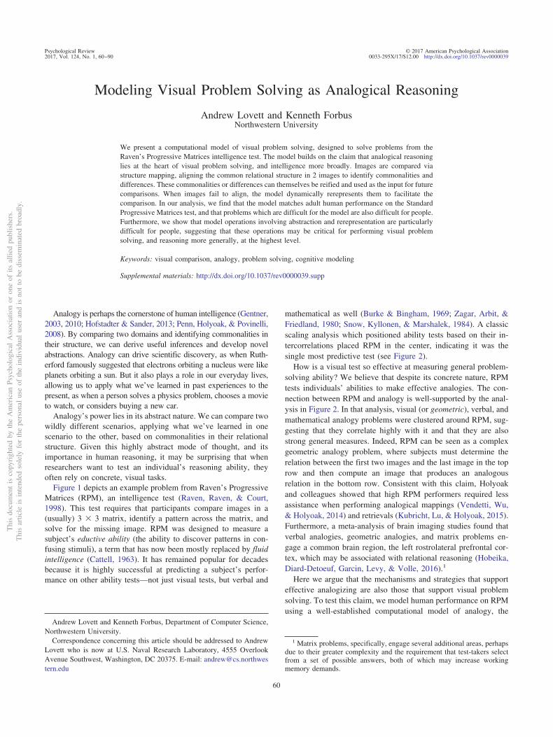
each object varied between images. Their analysis producedfive rules to explain how objects could vary: (a) constant in arow: the object stays the same; (b) quantitative pairwise pro-gression: the object changes in some way (e.g., rotating orincreasing in size) between images (Problem A, Figure 3); (c)distribution of three: there are three different objects in thethree images; those objects will be in every row, but their orderwill vary (Problem B); (d) figure subtraction or addition: add orsubtract the objects in the first two images to produce theobjects in the last (Problem E); and (e) distribution of two: eachobject is in only two of the three images (Problems F, H).Although the final rule sounds simple, it is actually quitecomplex. It requires recognizing that there is no correspondingobject in one of the three images.

Carpenter et al.’s (1990) FAIRAVEN model implements theserules. Given hand-coded, symbolic image representations as input,it analyzes each row via the following steps:

Figure 3. Example problems for various Carpenter et al. (1990) rules, and the strategy and abstractionoperation our model would use to solve each problem.

Thi

sdo

cum

ent

isco

pyri

ghte

dby

the

Am

eric

anPs

ycho

logi

cal

Ass

ocia

tion

oron

eof

itsal

lied

publ

ishe

rs.

Thi

sar

ticle

isin

tend

edso

lely

for

the

pers

onal

use

ofth

ein

divi

dual

user

and

isno

tto

bedi

ssem

inat

edbr

oadl

y.

62 LOVETT AND FORBUS

1. Identify corresponding objects. The model uses simpleheuristics, such as matching same-shaped objects, ormatching leftover objects.

2. For each set of corresponding objects, determine whichof the five rules (see above) it instantiates. FAIRAVENcan recognize every rule type except distribution of two.

The model performs these steps on each of the first two rowsand then compares the two rows’ rules, generalizing over them.Finally, it applies the rules to the bottom row to compute theanswer.

The BETTERAVEN model improves on FAIRAVEN in a fewways. First, during correspondence-finding, it can recognize caseswhere an object is only in two of the three images. Second, itchecks for the distribution of two rule. Third, it has a moredeveloped goal management system. It compares the rules identi-fied in the top two rows, and if they are dissimilar, it backtracksand looks for alternate rules.

Carpenter et al. (1990) argued that this last improvement, bettergoal management, was what truly set BETTERAVEN apart. Theybelieved that skilled RPM test-takers are adept at goal manage-

ment, primarily due to their superior work memory capacity. Thiscould explain RPM’s strong predictive power: it may accuratelymeasure working memory capacity, a key asset in other abilitytests. In support of this hypothesis, other researchers (Embretson,1998; Vodegel Matzen, van der Molen, & Dudink, 1994) havefound that as the number and complexity of Carpenter rules in aproblem increases, the problem becomes harder. Presumably, agreater number of rules places more load on working memory.

We believe Carpenter et al.’s (1990) models are limited in thatthey fail to capture perception, analogical mapping, and rerepre-sentation. As we have suggested above and argue below, theseprocesses are critical in both analogical thought and visual problemsolving. Because they do not analyze these or other general processes,Carpenter et al. can derive only limited connections between RPMand other problem-solving tasks. The primary connection they deriveis that RPM requires a high working memory capacity. Below, webriefly describe each of the model’s limitations.

1. Perception. The Carpenter et al. (1990) models takesymbolic representations as input. These representationsare hand-coded, based upon descriptions given by par-

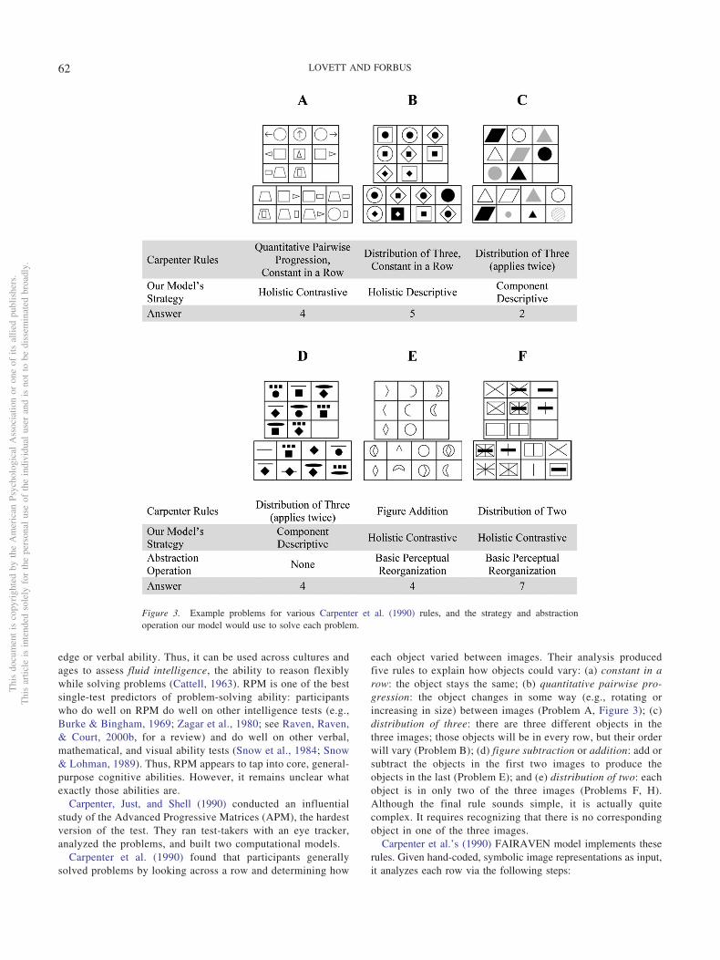
Figure 4. Two particularly difficult Raven’s problems.

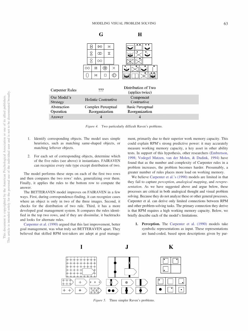
Figure 5. Three simpler Raven’s problems.

Thi

sdo

cum

ent

isco

pyri

ghte

dby

the

Am

eric

anPs

ycho

logi

cal

Ass

ocia

tion

oron

eof

itsal

lied

publ

ishe

rs.

Thi

sar

ticle

isin

tend

edso

lely

for

the

pers

onal

use

ofth

ein

divi

dual

user

and

isno

tto

bedi

ssem

inat

edbr

oadl

y.


ticipants. Although we agree on the use of symbolicrepresentations, this approach is limited in two respects:(a) it ignores the challenge of generating symbolic rep-resentations from visual input, and (b) it makes no the-oretical claims about what information should or shouldnot be captured in the symbolic representations. In fact,problem solving depends critically on what informationis captured in the initial representations, and the ability toidentify and represent the correct information might wellbe a skill underlying effective problem solving.

2. Analogical mapping. When the BETTERAVEN modelcompares images, it identifies corresponding objects us-ing three simple heuristics: (a) match up identical shapes,(b) match up leftover shapes, and (c) allow a shape tomatch with nothing. In contrast, we believe visual com-parison can use the same rich relational alignment pro-cess used in abstract analogies (Markman & Gentner,1996; Sagi et al., 2012).

In addition, we believe one challenge in RPM may bedetermining which images to compare. For example, inRPM it is typically enough to compare the adjacent imagesin each row, but for some problems one must also comparethe first and last images in the row (e.g., Problem E). In ouranalysis below, we test whether problems requiring thisadditional image comparison are more difficult to solve.

3. Rerepresentation. Carpenter et al. (1990) mention that insome cases their model is given a second representation totry if the first one fails to produce a satisfying answer. Thisis an example of rerepresentation: changing an image rep-resentation to facilitate a comparison. However, it appearsthat rerepresentation is not performed or analyzed in anysystematic way. In fact it is likely not needed in most casesbecause the initial representations are hand-coded—if theinitial representations are constructed to facilitate the com-parison, then no rerepresentation will be required.

We believe rerepresentation can play a critical role in visualproblem solving, as well as in analogy more broadly. In thispaper we show how rerepresentation is used to solve prob-lems such as G, and we analyze the difficulty of theseproblems for human test-takers.

Theoretical Framework

We argue that visual thinking often involves analogical pro-cessing of the same form that is used elsewhere in cognition

(e.g., Gentner & Smith, 2013; Kokinov & French, 2003). Thatis, a problem is encoded (perception) and analyzed to ascertainwhat comparison(s) are needed to be done. The comparisons arecarried out via structure mapping (Gentner, 1983). The resultsare analyzed and evaluated by task-specific processes, whichinclude methods for rerepresentation (Yan, Forbus, & Gentner,2003), often leading to further comparisons. This is an exampleof a map/analyze cycle (Falkenhainer, 1990; Forbus, 2001;Gentner et al., 1997), a higher-level pattern of analogical pro-cessing which has been used in modeling learning from obser-vation and conceptual change. The same overall structure, albeitwith vision-specific encoding and analysis processes, appears tobe operating in solving some kinds of visual problems, andspecifically RPM problems. This provides a straightforwardexplanation as to why RPM is so predictive of performance onso many nonvisual problems: The same processes are beingused.

One key claim which should be emphasized is: Rerepresen-tation is driven by comparison. Rather than a top– down searchprocess that explores different possible representations for eachimage, we are suggesting that initial, bottom– up representa-tions are changed only when necessary to facilitate a compar-ison.

Below we provide background on analogical mapping. We thendescribe five steps for visual problem solving:

1. Perception. Generate symbolic representations from im-ages.

2. Visual Comparison. Align the relational structure in twoimages, identify commonalities and differences.

3. Perceptual Reorganization. Rerepresent the images, ifnecessary, to facilitate a comparison.

4. Difference Identification. Symbolically represent thedifferences between images.

5. Visual Inference. Apply a set of differences to oneimage to infer a new image.

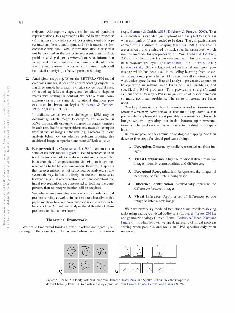
We have previously modeled two other visual problem-solvingtasks using analogy: a visual oddity task (Lovett & Forbus, 2011a)and geometric analogy (Lovett, Tomai, Forbus, & Usher, 2009; seeFigure 6). In what follows, we speak generally of visual problemsolving when possible, and focus on RPM specifics only whennecessary.

Figure 6. Panel A: Oddity task problem from Dehaene, Izard, Pica, and Spelke (2006). Pick the image thatdoesn’t belong. Panel B: Geometric analogy problem from Lovett, Tomai, Forbus, and Usher (2009).

Thi

sdo

cum

ent

isco

pyri

ghte

dby

the

Am

eric

anPs

ycho

logi

cal

Ass

ocia

tion

oron

eof

itsal

lied

publ

ishe

rs.

Thi

sar

ticle

isin

tend

edso

lely

for

the

pers

onal

use

ofth

ein

divi

dual

user

and

isno

tto

bedi

ssem

inat

edbr

oadl

y.


Analogical Mapping

Cases are represented symbolically, as entities, attributes, and re-lations. Two representations, a base and a target, are aligned based ontheir common relational structure (Doumas & Hummel, 2013; Gent-ner, 1983; Hummel & Holyoak, 1997; Larkey & Love, 2003). Basedon the corresponding attributes and relations, corresponding entitiescan be identified. The result of a mapping is a set of correspondencesbetween the base and target, and a similarity score based on the depthand breadth of aligned structure (Falkenhainer et al., 1989). Accord-ing to structure-mapping theory (Gentner, 1983, 2010), mappings areconstrained to allow each base item to map to just one target item.Mappings also include candidate inferences, where structure in onedescription is projected to the other. The results of a mapping can berepresented symbolically, so that they themselves can play a role infuture reasoning (even in future analogies). We use two types ofreification that have been used elsewhere in the literature for nonvi-sual comparisons:

1. Generalization. Here one constructs an abstraction,sometimes called a schema, describing the commonali-ties in the base and target (Glick & Holyoak, 1983;Kuehne, Forbus, Gentner, & Quinn, 2000).

2. Difference Identification. Here one explicitly representsthe differences between the base and target. The mostinteresting differences are alignable differences, wherethere is some expression in the base and some corre-sponding but different expression in the target (Gentner& Markman, 1994).

Visual Perception

To perform analogy between two stimuli, one must first gener-ate symbolic representations to describe them (Gentner, 2003,2010; Penn et al., 2008). Here we are interested not in low-levelvisual processing, but rather in the resulting representations andthe ways they can support problem solving. Visual representationscan be characterized as hierarchical hybrid representations(HHRs). They are hierarchical (Palmer, 1977; Marr & Nishihara,1978; Hummel & Stankiewicz, 1996) in that a given image can berepresented at multiple levels of abstraction in a spatial hierarchy;for example, a rectangle could be seen as a single object or as a setof four edges. They are hybrid in that there are separate qualitativeand quantitative components at each level in the hierarchy (Koss-lyn et al., 1989). The qualitative, or categorical component sym-bolically describes relations between elements; for example, oneobject contains another, or two edges are parallel (Biederman,1987; Forbus, Nielsen, & Faltings, 1991; Hummel & Biederman,1992). The quantitative component describes concrete quantitativevalues for each element, for example, its location, size, and ori-entation (Forbus, 1983; Kosslyn, 1996).

Qualitative representations are critical for helping us remember,reproduce, and compare spatial information (e.g., quadrants of a

circle: Huttenlocher, Hedges, & Duncan, 1991; angles between objectparts: Rosielle & Cooper, 2001; locations: Maki, 1982). We believethat these representations capture structural information about a visualscene, and that they can be compared via the same alignment pro-cesses used in analogy (Markman & Gentner, 1996; Sagi et al., 2012).However, as in any analogy, the outcome of the comparison dependsheavily on the representations used. In particular, one must select theappropriate level in the spatial hierarchy.

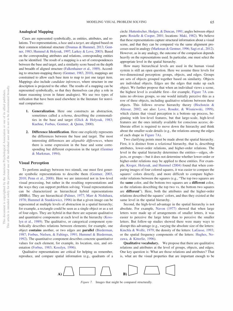
How many hierarchical levels are used in the human visualsystem is still an open question. Here we assume three levels fortwo-dimensional perception: groups, objects, and edges. Groupsare sets of objects grouped together based on similarity. Objectsare individual objects. Edges are the edges that make up eachobject. We further propose that when an individual views a scene,the highest level is available first—for example, Figure 7A con-tains no obvious groups, so one would initially perceive this as arow of three objects, including qualitative relations between theseobjects. This follows reverse hierarchy theory (Hochstein &Ahissar, 2002; see also: Love, Rouder, & Wisniewski, 1999),which claims that visual perception is a bottom–up process, be-ginning with low-level features, but that large-scale, high-levelfeatures are the ones initially available for conscious access; de-liberate effort is required to move down the hierarchy and thinkabout the smaller-scale details (e.g., the relations among the edgesof each shape in Figure 7A).

Two clarifying points must be made about the spatial hierarchy.First, it is distinct from a relational hierarchy, that is, describingattributes, lower-order relations, and higher-order relations. Thelevel in the spatial hierarchy determines the entities—edges, ob-jects, or groups—but it does not determine whether lower-order orhigher-order relations may be applied to these entities. For exam-ple, Kroger, Holyoak, and Hummel (2004) found that when com-paring images of four colored squares, it was easier to compare thesquares’ colors directly, and more difficult to compare higher-order relations between the squares (e.g., “The top two squares arethe same color, and the bottom two squares are a different color,so the relations describing the top two vs. the bottom two squaresare different”). Here, both the attributes and the higher-orderrelations described the squares’ colors, and thus they existed at thesame level in the spatial hierarchy.

Second, the high-level advantage in the spatial hierarchy is notabsolute. For example, Navon (1977) showed that when largeletters were made up of arrangements of smaller letters, it waseasier to perceive the large letter than to perceive the smallerletters. But follow-up studies showed there were many ways todisrupt this advantage (e.g., varying the absolute size of the letters:Kinchla & Wolfe, 1979; the density of the letters: LaGasse, 1993;or the spatial frequency components of the letters: Hughes, No-zawa, & Kitterlie, 1996).

Qualitative vocabulary. We propose that there are qualitativerelations and attributes at the level of groups, objects, and edges.One key question is: What are those relations and attributes? Thatis, what are the visual properties that are important enough to be

Figure 7. Images that might be compared structurally.

Thi

sdo

cum

ent

isco

pyri

ghte

dby

the

Am

eric

anPs

ycho

logi

cal

Ass

ocia

tion

oron

eof

itsal

lied

publ

ishe

rs.

Thi

sar

ticle

isin

tend

edso

lely

for

the

pers

onal

use

ofth

ein

divi

dual

user

and

isno

tto

bedi

ssem

inat

edbr

oadl

y.


captured qualitatively? Some qualitative relations are obvious (e.g.,one object is right of another, or one object contains another),whereas others are strongly supported by psychological evidence(e.g., concave angles between edges are highly salient: Ferguson,Aminoff, & Gentner, 1996; Hulleman, te Winkel, & Boselie, 2000).However, there is no straightforward way to produce a completequalitative vocabulary. Thus, our approach has been to consider theconstraints of the tasks we are modeling. We have developed aqualitative vocabulary that can be used across three different tasks:geometric analogy (Lovett et al., 2009), the visual oddity task (Lovett& Forbus, 2011a), and RPM. It can be viewed in its entirety at (Lovett& Forbus, 2011b). We see this vocabulary as one important outcomeof the modeling work, as it provides a set of predictions about humanvisual cognition. At the paper’s conclusion, we consider how thesepredictions can be further tested.

Visual Comparison

If visual perception produces a range of representations—qual-itative and quantitative components at different hierarchical levels—then visual problem solving consists of a strategic search throughthese representations, using comparison in order to find the keysimilarities and differences between two images. We view this searchas proceeding top–down and from qualitative to quantitative, thoughagain we do not claim that high-level representations are universallyaccessed first. At each step, the search is guided by analogical map-ping, which identifies corresponding elements in the two images.Next, we summarize top–down comparison and qualitative/quantita-tive comparison.

Top–down comparison. Oftentimes, comparisons at a highlevel in the spatial hierarchy can guide comparisons at a lowerlevel. Consider Figure 7. Each image contains three objects, andeach object contains four edges. Thus, an object-level representa-tion would consist of three entities, whereas an edge-level repre-sentation would consist of 12 entities. It is much simpler tocompare the objects than to compare the individual edges. How-ever, once the corresponding objects are known, the individualedges may be compared more easily.

A comparison between object-level representations, using analog-ical mapping, can identify the corresponding objects in the twoimages. In Figure 7, the leftmost trapezoid in image A goes with theleftmost trapezoid in image B because they occupy the same spot inthe relational structure. Once the corresponding objects are identified,one can compare the edge-level representations for each object pair.Thus, instead of comparing two images with 12 edges each, one iscomparing two objects with four edges each. These objects may becompared using the shape comparison strategy below.

Qualitative/quantitative comparison of shapes. This strat-egy identifies transformations between shapes, for example, therotation between trapezoids in Figure 7. It is inspired by research

on mental rotation, in which participants are shown two shapesand asked whether a rotation of one would produce the other(Shepard & Metzler, 1971; Shepard & Cooper, 1982). A popularhypothesis is that people perform an analog rotation in their minds,transforming one object’s representation to align it with the other.Our approach assumes the existence of two representations: aqualitative, orientation-invariant representation that describes theedges’ locations and orientations relative to each other; and aquantitative, orientation-specific representation that describes theabsolute location, orientation, size, and curvature of each edge. Itworks as follows (Lovett et al., 2009):

1. Using structure mapping, compare qualitative, orientation-invariant representations for the two shapes. This willidentify corresponding parts in the shapes. For example,comparing the two leftmost shapes, the lower edge inFigure 7A goes with the leftmost edge in 7B.

2. Take one pair of corresponding parts. Compute a quan-titative transformation between them. Here, there is a 90°clockwise rotation between the two edges.

3. Apply the quantitative transformation to the first shape.Here, we rotate the shape 90°. After the rotation iscomplete, compare the aligned quantitative representa-tions to see if the locations, sizes, orientations, and cur-vatures of the corresponding edges match.

Perceptual Reorganization

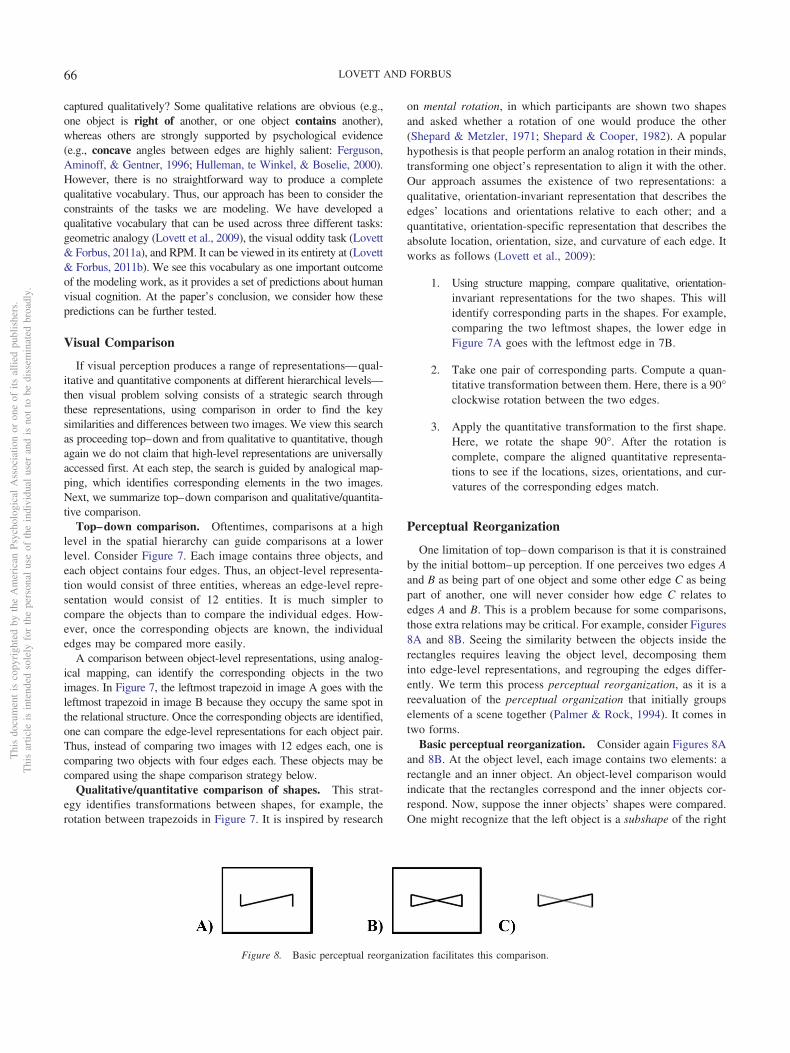
One limitation of top–down comparison is that it is constrainedby the initial bottom–up perception. If one perceives two edges Aand B as being part of one object and some other edge C as beingpart of another, one will never consider how edge C relates toedges A and B. This is a problem because for some comparisons,those extra relations may be critical. For example, consider Figures8A and 8B. Seeing the similarity between the objects inside therectangles requires leaving the object level, decomposing theminto edge-level representations, and regrouping the edges differ-ently. We term this process perceptual reorganization, as it is areevaluation of the perceptual organization that initially groupselements of a scene together (Palmer & Rock, 1994). It comes intwo forms.

Basic perceptual reorganization. Consider again Figures 8Aand 8B. At the object level, each image contains two elements: arectangle and an inner object. An object-level comparison wouldindicate that the rectangles correspond and the inner objects cor-respond. Now, suppose the inner objects’ shapes were compared.One might recognize that the left object is a subshape of the right

Figure 8. Basic perceptual reorganization facilitates this comparison.

Thi

sdo

cum

ent

isco

pyri

ghte

dby

the

Am

eric

anPs

ycho

logi

cal

Ass

ocia

tion

oron

eof

itsal

lied

publ

ishe

rs.

Thi

sar

ticle

isin

tend

edso

lely

for

the

pers

onal

use

ofth

ein

divi

dual

user

and

isno

tto

bedi

ssem

inat

edbr

oadl

y.


object. That is, all the edges in the left object are also found in theright object.

Based on this finding, one could update Figure 8B’s represen-tation, segmenting the inner object into two objects (Figure 8C).Now, when the two images are compared, one can better see howthe images relate to each other: the right image contains the leftimage, plus an additional edge.

Complex perceptual reorganization. Sometimes, the strategyabove is not enough. Consider Figure 9. At the object level, the leftimage might contain two objects: a square and an ‘X;’ and the rightimage might contain a single object: an hourglass. Suppose the initialcomparison aligned the square with the hourglass. These are com-pletely different shapes, so at this stage, the relation between theimages is poorly understood. Furthermore, because neither shape is asubshape of the other, basic perceptual reorganization is not an option.

However, one might recognize that the corresponding objectsshare some common parts: horizontal edges at the top and bottom.With this strategy, one explores these commonalities by breakingeach object down into its parts. The objects are segmented intoseparate entities for each edge, and the comparison is repeated.Now, suppose the X shape in the left image corresponds to one ofthe diagonals in the right image. Again, they share a common part,so the X shape is broken down into its edges.

When the comparison is repeated, one gets a set of correspond-ing edges in the two images: the two diagonals correspond, and thetop and bottom horizontal edges correspond. Because these edgesare common across the two images, one can group them backtogether into a single object. This produces three objects in the leftimage: an hourglass, and the two vertical edges. It produces oneimage in the right object: an hourglass. Finally, the comparison isrepeated, and a new understanding emerges: the left image con-tains the right image, plus vertical edges on its right and left sides.

Complex reorganization requires more steps than basic reorga-nization. It places greater demands on an individual’s abstractionability; in this example, one must move fluidly between the objectand edge levels. It also places greater demands on working mem-ory; to solve Figure 9, one must consider all the edges at once,rather than merely the edges in each object. Thus, we would expectcomparisons involving complex perceptual reorganization to re-quire significantly more effort than comparisons involving basicperceptual reorganization.

Difference Identification

Both geometric analogy and RPM problems require an individ-ual to compare images and identify the key differences betweenthem—in other words, how are the objects changing betweenImages A and B in a geometric analogy problem (Figure 6B), oracross a row of images in an RPM problem (Carpenter et al.,1990). We use the term pattern of variance for a symbolic,qualitative representation of the differences across two or moreimages. Differences may include:

1. Spatial relations being added, removed, or reversed. InFigure 6B, a contains relation is removed and a right ofrelation is added between A and B.

2. Objects being added, removed, or transformed. In Figure6B, the dot shape is removed.

Top–down comparison provides an effective means for com-puting patterns of variance. Analogical mapping identifies changesin the relational structure, or objects in one image that have nocorresponding object in another image. Shape comparison identi-fies transformations, such as when an object rotates.

Patterns of variance may be reminiscent of transformationaldistance models of similarity, where two stimuli are compared bycomputing the transformations between them (e.g., Hahn, Chater,& Richardson, 2003). However, they are distinct in that patterns ofvariance are the result of the comparison, and not the actualmechanism of comparison.

Patterns of Variance in RPM

RPM is unique among the tasks we’ve considered in that itrequires computing patterns of variance across rows of threeobjects. These patterns can be complex, and identifying the correctpattern type is critical to solving the problems (Carpenter et al.,1990). We propose that the patterns may be characterized via twobinary parameters, resulting in four pattern types. Consider theexample problems in Figure 3.

Contrastive/descriptive patterns. Many RPM problems in-volve the objects changing in some way as you look across each rowof the matrix. For example, in Problem A, one object moves from theleft to the right side of the other object, while it rotates clockwise.Each row of Problem A could be represented with a contrastivepattern of variance which captures these changes. On the other hand,other problems involve some set of objects appearing in each row. InProblem B, each row contains a square, a circle, and a diamond,although the order in which these appears varies across rows. Theserows each could be represented with a descriptive pattern of variance,which simply describes each image in the row.

Although a descriptive pattern doesn’t explicitly describe differ-ences, it is sensitive to them. In the top row of Problem B, there is aninner circle in each image. Because this circle does not change acrossthe images of the row, it is not included in the pattern of variance.Thus, the pattern only describes the square, circle, and diamondshapes, which are the key information needed to solve the problem.

Holistic/component patterns. Patterns may also be classifiedas holistic or component. The examples given above are holisticpatterns, where differences between entire images are represented. Incomponent patterns, images must be broken down into their compo-nent elements, which are represented independently. For example,Problem D requires a component descriptive pattern which essentiallysays: “Each row contains a circle, a square, and a diamond. Indepen-dently, each row also contains a group of squares, a horizontal line,and an ellipse.” Which objects are paired together in the images willvary across rows, and so it cannot be a part of the pattern.

A given matrix row can be represented using any of the four patterntypes. Thus, to determine if one has chosen the correct type, one mustcompare the patterns for the top and middle rows. This can be doneusing the same analogical mapping process. If the patterns align, thisFigure 9. Complex perceptual reorganization facilitates this comparison.

Thi

sdo

cum

ent

isco

pyri

ghte

dby

the

Am

eric

anPs

ycho

logi

cal

Ass

ocia

tion

oron

eof

itsal

lied

publ

ishe

rs.

Thi

sar

ticle

isin

tend

edso

lely

for

the

pers

onal

use

ofth

ein

divi

dual

user

and

isno

tto

bedi

ssem

inat

edbr

oadl

y.


confirms that the rows are being represented correctly. If not, it will benecessary to backtrack and represent the rows differently.

One open question is whether some pattern types are moredifficult to represent than others. In particular, as the patternsbecome more abstract and farther from the initial concrete images,will they be processed less fluently (Kroger et al., 2004)? Com-paring contrastive and descriptive patterns, contrastive patternsappear more abstract, as they describe the differences betweenimages, rather than the contents of each image. Comparing holisticand component patterns, component patterns appear more abstract,as they isolate each object from the image in which it appeared.The simulation below presents an opportunity to compare thesepattern types and determine their relative difficulty.

Visual Inference

Finally, a set of differences can be applied to one image to infera new image. Consider our geometric analogy example (Figure6B). First, Images A and B are compared with compute a patternof variance between them, as described above. Next, Images A andC are compared to identify the corresponding objects. Finally, theA/B differences are applied to image C to infer D’, a representationof the answer image. In this case, the dot is removed and the Zshape is moved to the left of the pie shape. Note that because thisinference is performed on qualitative, symbolic representations, theresulting D’ is another representation, not a concrete image. Thus, theproblem-solver can infer that the Z shape should be on the left, butthey may not know the exact, quantitative locations of the objects.

Visual inference can also be performed on the patterns ofvariance in RPM. Consider Problem A (see Figure 3). The patternof variance for the top row indicates that one object moves to theright while rotating clockwise. By comparing the images in the topand bottom rows, one can determine that the arrow maps to therectangle, and the circle maps to the trapezoid. Thus, one infersthat in the answer image, the rectangle should move to the right ofthe trapezoid and rotate clockwise.

Note that the above strategy is not the only way to solve ProblemA. Alternatively, one might use a second-order comparison strategy:(a) Compare images in the top row, compute a pattern of variance; (b)for each possible answer, insert it into the bottom row and compute apattern of variance; and (c) compare the top row pattern to eachbottom row pattern, and pick the answer that produces the closest fit.Later, we use the model to explain why people might use a visualinference strategy or a second-order comparison strategy.

Model

Our computational model builds on the above claims, in particular:(a) analogy drives visual problem solving, (b) hierarchical hybridrepresentations (HHRs) capture visual information, and (c) problemsolving is a strategic search through the representation space. Ifinterested, the reader may download the computational model and runit on example Problems A–K.2 The model possesses two keystrengths:

1. The model is not strongly tied to Raven’s Matrices. Ituses the Structure-Mapping Engine, a general computa-tional model of analogy, and it incorporates operationsthat have been used to model other visual problem-solving tasks, including geometric analogy (Lovett &Forbus, 2012) and the visual oddity task (Lovett & For-bus, 2011a). Furthermore, the visual representations usedhere are identical to those used in the geometric analogymodel, and nearly identical to those used in the odditytask model.3 Thus, this model allows us to test thegenerality of our claims.

2. The model possesses multiple strategies for solving aproblem. One strategy solves the simpler, more visualproblems found in the first section of the Standard Pro-gressive Matrices (SPM) test (e.g., Problem I). The othertwo strategies, described in the next section, capturealternative approaches for solving typical 3 � 3 prob-lems. Although including both strategies is not necessaryfor solving the problems, it allows us to more fully modelthe range of human problem-solving behavior.

This section is divided up as follows. First, we provide anoverview of how the model solves problems, walking throughseveral examples and covering the special cases where a 3 � 3matrix is not used (example Problems I, J, and K). Second, wesummarize the existing systems on which the model is built. Third,we describe the basic operations used to model RPM and other

2 See http://www.qrg.northwestern.edu/software/cogsketch/CogSketch-v2023-ravens-64bit.zip (Windows only). The reader may also downloadthe source code for the model. http://dx.doi.org/10.1037/rev0000039.supp

3 The only difference from the oddity task model is the inclusion of anattribute describing the relative size of an object. This attribute has beenincluded in later versions of the oddity task model.

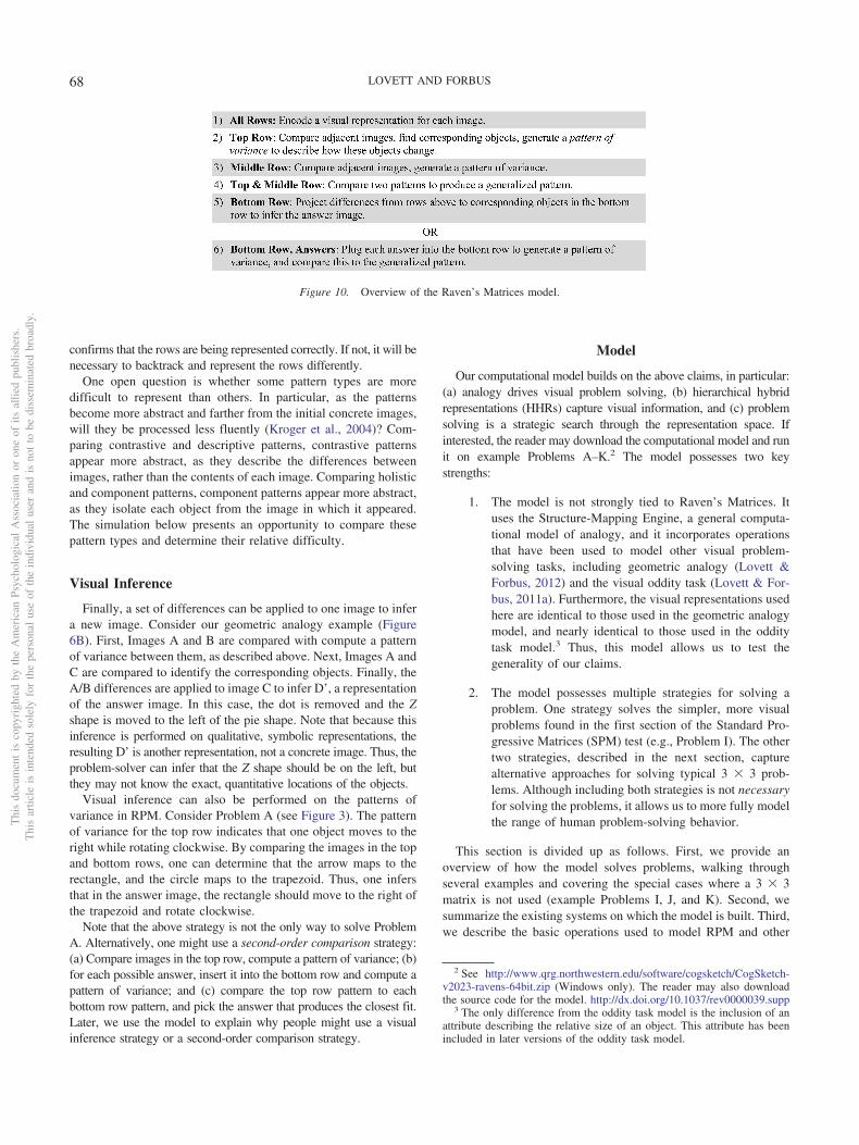
Figure 10. Overview of the Raven’s Matrices model.

Thi

sdo

cum

ent

isco

pyri

ghte

dby

the

Am

eric

anPs

ycho

logi

cal

Ass

ocia

tion

oron

eof

itsal

lied

publ

ishe

rs.

Thi

sar

ticle

isin

tend

edso

lely

for

the

pers

onal

use

ofth

ein

divi

dual

user

and

isno

tto

bedi

ssem

inat

edbr

oadl

y.


http://www.qrg.northwestern.edu/software/cogsketch/CogSketch-v2023-ravens-64bit.zip

http://www.qrg.northwestern.edu/software/cogsketch/CogSketch-v2023-ravens-64bit.zip

http://dx.doi.org/10.1037/rev0000039.supp

visual problem-solving tasks. Fourth, we cover the strategic deci-sions the model must make during problem solving. As we shallsee, the difficulty of a problem depends greatly on the outcome ofthe strategic decisions, and thus they allow us to explore whatmakes a problem difficult and what makes an individual an effec-tive problem-solver.

Figure 10 illustrates the steps the model takes to solve 3 � 3matrix problems. Each problem is solved through a series ofcomparisons, first comparing the images in a row to generate apattern of variance that describes how the images are changing,then comparing the patterns in the top two rows. Each of thesecomparisons requires a strategic search for the representation thatbest facilitates the comparison. Finally, the model solves a prob-lem using one of two strategies: visual inference (step 5) orsecond-order comparison (step 6). Below, we walk through thesteps using Problems A, D, and G as examples.

Step 1

The model automatically generates a representation for eachimage in the problem (i.e., each cell of the matrix). The modelgenerates the highest-level representation possible, focusing on thebig picture (e.g., groupings of objects), rather than the small details(edges within each object). Each representation includes a list ofobjects and set of qualitative relations between the objects, as wellas qualitative features for each object. The set of qualitativerelations and features is known as a structural representation, andit allows two images to be compared via structure mapping.

In Problem A, the upper leftmost image representation wouldindicate that there are two objects, one open and one closed. Theclosed object is right of the open object. The closed object iscurved and symmetrical (this is just a sampling of the represen-tation). In Problem D, the three squares in the upper leftmostimage would be grouped together based on similarity. The repre-sentation would describe a group which is located above anobject. In the Problem G, the representation would include twoobjects: an ellipse and an X shape inside the ellipse.

Step 2

The adjacent images in the top row are compared via top–downcomparison: first the images are compared to identify correspond-ing objects, and then the corresponding objects are compared toidentify shape changes and transformations. The full set of differ-ences is encoded as a pattern of variance: a qualitative, symbolicrepresentation of what is changing between the images.

In Problem A, the pattern indicates that an object moves fromleft of to within to right of another object while rotating. InProblem D, the pattern indicates that the objects are entirelychanging their shapes between each image. In Problem G, thepattern, which matches the ellipse shape to an hourglass shape toa simpler, squared-off hourglass shape, is largely unsatisfying.However, the comparison indicates that corresponding objectshave some parts in common (the vertical and diagonal edges).Therefore, the model initiates complex perceptual reorganization,breaking the objects down into their component edges. Groupingthe corresponding edges backup, it determines that each imagecontains the squared-off hourglass shape found in the rightmostimage. Thus, the change is that there are first two horizontal

curves, then two vertical curves, then neither, while the squared-off hourglass remains the same.

Step 3

The same steps are performed for the middle row.

Step 4

The patterns of variance for the top two rows are compared viastructure mapping. A generalized pattern consisting of the com-mon elements to both rows is generated.

In Problem A, the rows are a perfect match: they both contain anobject moving to the right and rotating. Similarly, in Problem Gthey both contain two horizontal curves, then two vertical curves,then neither. In Problem D, however, there is a bad match: in thetop row, there is a change from circle to square, whereas in themiddle row there is a change from diamond to circle (as describedbelow, the model does not know terms like “square,” but it is ableto distinguish different shapes). Thus, the model must searchthrough the range of possible representations for a pattern ofvariance.

The typical representation is a holistic contrastive representa-tion, which represents the changes between each image. Here, themodel gets better results with a component descriptive represen-tation. It is descriptive in that it describes what it sees, rather thandescribing changes. For example, in the top row, it sees a circle, soit expects to find a circle somewhere in the middle row. It iscomponent in that it does not group objects together in images. Thecircle and the group of square are in the same image in the top row,but it does not expect to find them in the same image in the nextrow. Essentially, the representation says that in each row there isa circle, a square, and a diamond; and also a group, a horizontaledge, and an ellipse. Using this representation, the model finds aperfect fit between the rows.

Step 5

When possible, the model attempts to solve problems via visualinference. It projects the differences to the bottom row and infersthe answer image. This first requires finding correspondencesbetween the bottom row objects and objects in a row above, againusing structure mapping.

In Problem A, the trapezoid and rectangle in the bottom rowcorrespond to the circle and arrow in the top row (based oncorresponding relational structure).4 The model infers that in themissing image, the rectangle should be to the right of the trapezoid,and it should be rotated 90° from its orientation in the middleimage. In Problem B, the objects in the bottom row correspond tothe objects in the top row. The missing objects are a circle and ahorizontal edge, so the model infers that the answer should containthese objects.

In Problem G, the inference fails. The model required all threeimages to perform complex perceptual reorganization on the aboverows, suggesting that all three images will be needed for a similar

4 Either the top or middle row can be compared with the incompletebottom row. The model actually uses whichever is closest to the bottomrow, in terms of number of elements per image.

Thi

sdo

cum

ent

isco

pyri

ghte

dby

the

Am

eric

anPs

ycho

logi

cal

Ass

ocia

tion

oron

eof

itsal

lied

publ

ishe

rs.

Thi

sar

ticle

isin

tend

edso

lely

for

the

pers

onal

use

ofth

ein

divi

dual

user

and

isno

tto

bedi

ssem

inat

edbr

oadl

y.


perceptual reorganization on the bottom row. Without knowing thethird image in the bottom row, the model abandons the visualinference strategy. Another approach must be used to solve for theanswer.

Step 6

When visual inference fails, the model falls back on a simplerstrategy: second-order comparison. It iterates over the list ofanswers and plugs each answer into the bottom row, computing thebottom row’s pattern of variance. It selects the answer whoseassociated pattern best matches the generalized pattern for theabove rows.

In Problem G, the model selects answer 4 because when the Xis plugged into the bottom row, it produces a similar pattern of twohorizontal curves, then two vertical curves, then neither.

The visual inference and second-order comparison approachesmap onto classic strategies for analogical problem solving. Psy-chologists and modelers studying geometric analogy (“A is to B asC is to . . . ?”) have argued over whether people solve directly forthe answer (Sternberg, 1977; Schwering, Gust, Kühnberger, &Krumnack, 2009) or evaluate each possible answer (Evans, 1968;Mulholland, Pellegrino, & Glaser, 1980), with some (Bethell-Fox,Lohman, & Snow, 1984) suggesting that we adjust our strategydepending on the problem. We previously showed how a geomet-ric analogy model incorporating both strategies could better ex-plain human response times (Lovett & Forbus, 2012).

Here, we model both strategies not because both are required—the Carpenter model used visual inference exclusively, whereasour own model could use second-order comparison exclusivelywithout a drop in performance. Rather, we hope to better explainhuman performance by incorporating a greater range of behavior.Following our geometric analogy model, this model attempts tosolve for answers directly via visual inference. When this fails, itreverts to second-order comparison. In our analysis, we considerwhether people have greater difficulty on the problems where thishappens.

Solving 2 � 2 Matrices

The Standard Progressive Matrices (SPM) includes simpler 2 �2 matrices (e.g., Problem K) which lack a middle row. Becausethere is no way to evaluate the top row representation, the modelsimply assumes that a contrastive representation is appropriate,skipping Steps 2 and 3 above. Problem solving is otherwise thesame.

Solving Nonmatrix Problems

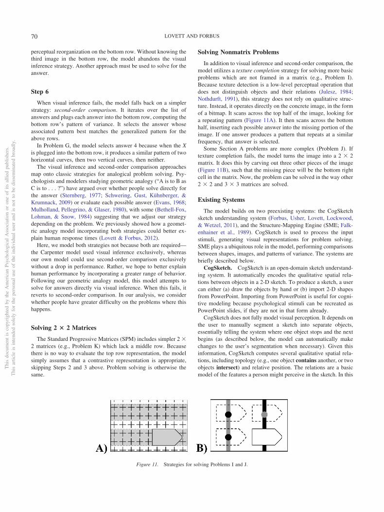
In addition to visual inference and second-order comparison, themodel utilizes a texture completion strategy for solving more basicproblems which are not framed in a matrix (e.g., Problem I).Because texture detection is a low-level perceptual operation thatdoes not distinguish objects and their relations (Julesz, 1984;Nothdurft, 1991), this strategy does not rely on qualitative struc-ture. Instead, it operates directly on the concrete image, in the formof a bitmap. It scans across the top half of the image, looking fora repeating pattern (Figure 11A). It then scans across the bottomhalf, inserting each possible answer into the missing portion of theimage. If one answer produces a pattern that repeats at a similarfrequency, that answer is selected.

Some Section A problems are more complex (Problem J). Iftexture completion fails, the model turns the image into a 2 � 2matrix. It does this by carving out three other pieces of the image(Figure 11B), such that the missing piece will be the bottom rightcell in the matrix. Now, the problem can be solved in the way other2 � 2 and 3 � 3 matrices are solved.

Existing Systems

The model builds on two preexisting systems: the CogSketchsketch understanding system (Forbus, Usher, Lovett, Lockwood,& Wetzel, 2011), and the Structure-Mapping Engine (SME; Falk-enhainer et al., 1989). CogSketch is used to process the inputstimuli, generating visual representations for problem solving.SME plays a ubiquitous role in the model, performing comparisonsbetween shapes, images, and patterns of variance. The systems arebriefly described below.

CogSketch. CogSketch is an open-domain sketch understand-ing system. It automatically encodes the qualitative spatial rela-tions between objects in a 2-D sketch. To produce a sketch, a usercan either (a) draw the objects by hand or (b) import 2-D shapesfrom PowerPoint. Importing from PowerPoint is useful for cogni-tive modeling because psychological stimuli can be recreated asPowerPoint slides, if they are not in that form already.

CogSketch does not fully model visual perception. It depends onthe user to manually segment a sketch into separate objects,essentially telling the system where one object stops and the nextbegins (as described below, the model can automatically makechanges to the user’s segmentation when necessary). Given thisinformation, CogSketch computes several qualitative spatial rela-tions, including topology (e.g., one object contains another, or twoobjects intersect) and relative position. The relations are a basicmodel of the features a person might perceive in the sketch. In this

Figure 11. Strategies for solving Problems I and J.

Thi

sdo

cum

ent

isco

pyri

ghte

dby

the

Am

eric

anPs

ycho

logi

cal

Ass

ocia

tion

oron

eof

itsal

lied

publ

ishe

rs.

Thi

sar

ticle

isin

tend

edso

lely

for

the

pers

onal

use

ofth

ein

divi

dual

user

and

isno

tto

bedi

ssem

inat

edbr

oadl

y.


work, we use CogSketch to simplify perception and problemsolving in three ways:

1. Each RPM problem is initially manually segmented intoseparate objects. Problems are recreated in PowerPoint,drawing one PowerPoint shape for each object,5 and thenimported into CogSketch. The experimenters attempt tosegment each image into objects consistently, based onthe Gestalt grouping rules of closure and good continu-ation (Wertheimer, 1938), that is, preferring closedshapes and longer straight lines. We note that the systemmay revise this segmentation based on its automaticgrouping processes, and based upon perceptual reorgani-zation.

2. For nonmatrix problems (e.g., Problems I–J), the large,upper rectangle is given the label “Problem” within Cog-Sketch. The smaller shape within this rectangle that sur-rounds the missing piece is given the label “Answer.”The model uses this information to locate these objectsduring problem solving.

3. Each RPM problem is segmented into separate images(i.e., the cells of the matrix and the list of possibleanswers) using sketch-lattices. A sketch-lattice is an N �N grid that can be overlaid on a sketch. Each cell of thegrid is treated as a separate image, for the purposes ofcomputing image representations. Sketch-lattices can beused to locate particular images (e.g., the upper leftmostimage in the top sketch-lattice). RPM problems requiretwo sketch-lattices: one for the problem matrix, and onefor the list of possible answers.

CogSketch’s objects are the starting point for our model’sperceptual processing. The model automatically forms higher-levelrepresentations by grouping objects together and lower-level rep-resentations by segmenting objects into their edges. It supplementsCogSketch’s initial spatial relations to form a complete HHR foreach image.

Structure-Mapping Engine

SME is a computational model of comparison based onstructure-mapping theory. It operates on structured representationsorganized as predicate calculus statements (e.g., (right ofObject-A Object-B)). Given two representations, it aligns theircommon structure to compute a mapping between them. A map-ping consists of (a) a set of correspondences, (b) a similarity score,and (c) candidate inferences based on carrying over unmatchedstructure. For this work, we used a normalized similarity score,ranging from 0 to 1. Note that SME is domain-general—it operateson visual representations as easily as more abstract conceptualrepresentations.

One important feature in SME is the ability to specify matchconstraints, rules that affect what can be matched with what. Forexample, a user may specify that entities with a particular attributecan only match with other entities that share that attribute. In thevisual domain, one can imagine a variety of possible match con-straints (only allow objects with the same color, or size, or shapeto match, etc.). To support creative reasoning and comparison, our

model uses no match constraints in its initial comparisons. Asdescribed below, it dynamically adds constraints when necessaryas part of the problem-solving process.

Model Operations

The RPM model builds on a set of operations which havepreviously been used to solve other visual problem-solving tasks.Figure 12 illustrates the operations used at each step in the process(compare with Figure 10). Below, we describe each operation,including its input, its output, and any additional options availablewhen performing the operation (e.g., the option of representingeither a contrastive or descriptive pattern of variance). In thefollowing section, we discuss the key strategic decisions maderegarding these options at each step.

See the Appendix for additional details on how each operationis implemented.

Encode. Given an image, this produces a qualitative, struc-tural representation at a particular level in the spatial hierarchy(Edges, Objects, or Groups). The representation contains a list ofelements and a list of symbolic expressions. For example, anobject-level representation would list the objects in an image andinclude relations like (right of Object-A Object-B). An edge-levelrepresentation would list the edges in an object and include rela-tions like (parallel Edge-A Edge-B). A group-level representationwould include any groups that could be formed (e.g., a row ofidentical shapes could be grouped together) but otherwise beidentical to the object level. Note that objects may include closedshapes (e.g., a circle), open shapes (e.g., an X), texture patches (agrouping of parallel edges), and negative space. See the Appendixfor more details.

Additional options. The level of the desired representation(Edges, Objects, or Groups) can be specified. Note that the RPMmodel, in keeping with HHRs, begins by representing at thehighest level, Groups, because representations are sparser andeasier to compare at this level.

Compare Shapes. This operation takes two elements andcomputes a transformation between them by comparing theirparts—that is, it compares the edges in two objects or the objectsin two groups. Like the other comparison operations (see below),it compares qualitative, structural representations using SME.

Compare Shapes can produce shape transformations, shapedeformations, and group transformations. The shape transfor-mations are rotations, reflections, and changes in scale. Theshape deformations are lengthening, where two edges along acentral axis grow longer (Figure 13A); part-lengthening, wheretwo edges along a part of the object grow longer (13B); part-addition, where a new part is added to the object (13C), and thesubshape deformation, where two objects are identical, exceptthat one has extra edges (used to trigger basic perceptualreorganization, as in Figure 8).

The group transformations are identical groups, larger group(similar to subshape where two groups are identical except thatone has more objects), different groups (where groups have dif-ferent arrangements of the same objects), and object to group

5 Some objects cannot be drawn as a single shape, due to PowerPoint’slimitations. These are drawn as multiple shapes, imported into CogSketch,and then joined together using CogSketch’s merge function.

Thi

sdo

cum

ent

isco

pyri

ghte

dby

the

Am

eric

anPs

ycho

logi

cal

Ass

ocia

tion

oron

eof

itsal

lied

publ

ishe

rs.

Thi

sar

ticle

isin

tend

edso

lely

for

the

pers

onal

use

ofth

ein

divi

dual

user

and

isno

tto

bedi

ssem

inat

edbr

oadl

y.


(where a single object maps to a group of similar objects). As withsubshape, the larger group and object to group transformationsmay serve as triggers for basic perceptual reorganization.

Recognize Shape. This operation assigns a shape categorylabel to an object. Although the model has no preexisting knowl-edge of shape types (e.g., “square”), it can learn categories for theshapes found within a particular problem. Shapes are grouped intothe same category if there is a valid transformation between them(scaling � rotation or reflection). When a new element is encoun-tered, it is recognized by comparing it to an exemplar from eachshape category. If it does not match any category, a new categoryis created.

Objects may be assigned arbitrary labels for their shape catego-ries, which apply only in a particular problem context (e.g., allsquares might be assigned the category “Type-1” within the con-text of solving a problem).

Compare Images. Given two image representations, Com-pare Images performs top–down comparison. First, it comparesthe image representations with SME to find the correspondinggroups or objects. Then, it calls Compare Shapes on those corre-sponding elements, in order to compute any shape transformations.It returns (a) a similarity score for the two images, computed bySME but modified based on whether corresponding elements arethe same shape; (b) a set of corresponding elements; (c) a set ofcommonalities, based on those parts of the representations thataligned during the SME mapping; and (d) a set of differences.

There are three types of differences: (a) changes in the relationalstructure, found by SME, for example, a change from (aboveObject-A Object-B) to (right of Object-A Object-B); (b) additionsor removals of elements between the images (i.e., when an objectis present in one image but absent in the next); and (c) shape

transformations between the images (see Compare Shapes abovefor a list of possible shape transformations). In some cases, anobject may change shape entirely, as when a square maps to acircle. In this case, the transformation is encoded as a changebetween the two shapes’ category labels.

Find Differences. This operation compares a sequence ofimages, using Compare Images, and produces a pattern of vari-ance, a structural representation of the differences between them(see the previous section for a list of possible difference types). Forexample, suppose Find Differences was called on the top row inProblem A. It would compare adjacent images (the left and middleimages, and the middle and right images), identifying the corre-sponding objects. Here, the circle shapes correspond and the arrowshapes correspond. It would then encode the changes betweenadjacent images, using the differences from Compare Images.Between the first two images, the circle shape changes from beingright of the arrow to containing the arrow. Also, the arrow rotates90°. Between the next two images, the arrow moves to the right ofthe circle and rotates again.

Additional options. As discussed above, much of the strategyin RPM relates to rows of images: how they should be compared,and how their differences should be represented. Find Differencessupports several strategic choices regarding how images are com-pared:

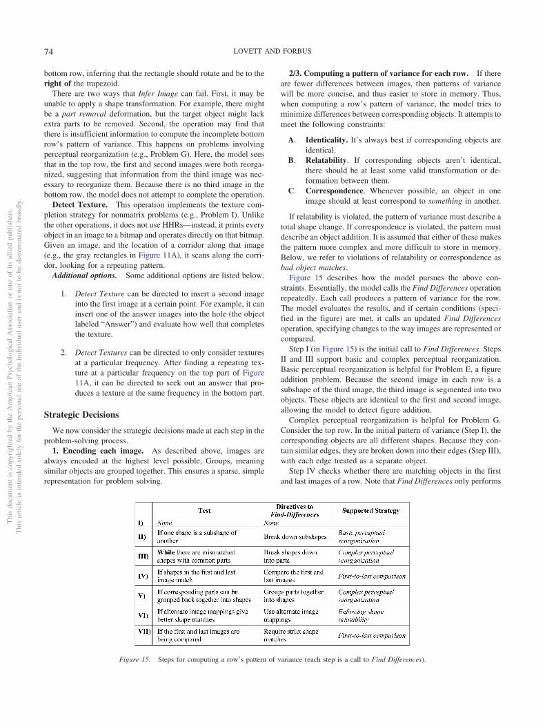
1. Basic perceptual reorganization can be triggered, basedon one object (or group) being a subshape of another. Forthe top row of Problem E, the middle object is a subshapeof the right object, so the right object can be segmentedinto objects, one identical to the middle object and oneidentical to the left object.

Figure 12. Overview of the Raven’s Matrices model with operations.

Figure 13. Examples of shape deformations.

Thi

sdo

cum

ent

isco

pyri

ghte

dby

the

Am

eric

anPs

ycho

logi

cal

Ass

ocia

tion

oron

eof

itsal

lied

publ

ishe

rs.

Thi

sar

ticle

isin

tend

edso

lely

for

the

pers

onal

use

ofth

ein

divi

dual

user

and

isno

tto

bedi

ssem

inat

edbr

oadl

y.


2. Complex perceptual reorganization can be triggered,based on two objects (or groups) sharing common parts.This is used in Problem G.

3. First-to-last comparison can be performed. That is, thefirst and last images can be compared, even though theyare not adjacent. For the top row in Problem H, thisallows one to see that the curved edge in the left imagematches the curved edge in the right image.

4. Strict shape matching can be enforced for some or allshape categories. This means the SME mapping is con-strained to only allow identically shaped objects to matcheach other. This is paired with first-to-last comparison. InProblem H, it would ensure that the curved edge in theleft image doesn’t map to anything in the middle image.Thus, Find Differences would determine that there is anobject present in the first and last image, but not themiddle image.

Find Differences also supports two strategic decisions for how arow’s pattern of variance is represented, once it has been com-puted.

1. A pattern can be contrastive or descriptive. A contrastivepattern represents the differences between each adjacentpair of images, whereas a descriptive pattern describeseach image, abstracting out features that are commonacross the images. Shape labels from Recognize Shapeare used to capture information such as “This row con-tains a square, a circle, and a diamond.” Typically acontrastive pattern includes ordering information, indi-cating the first second and third images in a row, while adescriptive pattern does not.

2. A pattern can be holistic or component. A holistic patternrepresents the row in terms of images, including whatchanges between images (contrastive) or what is presentin each image (descriptive). Alternatively, a componentpattern ignores the overall images and represents howeach individual object changes (contrastive) or what ob-jects are present in the row (descriptive).

If every image contains only a single object, then a componentdescriptive pattern breaks the objects down into their features andrepresents those separately. In Problem C, each row contains aparallelogram, a circle, and a triangle; and a black object, a whiteobject, and a gray object.

A component pattern of variance is the most abstract kind,because it abstracts out the image itself. Two things necessarilyfollowing from this: (a) ordering is not constrained, as there are noimages to order and (b) spatial relations are not represented, asobjects are no longer tied together in an image.

Generalize. Like Find Differences, this operation comparestwo or more items via SME. However, instead of encoding thedifferences, it encodes the commonalities, that is, the attributes andrelations that successfully align. It returns (a) a similarity score,computed by SME and (b) a new representation, containing thecommonalities in the compared representations, that is, the expres-sions that successfully aligned.

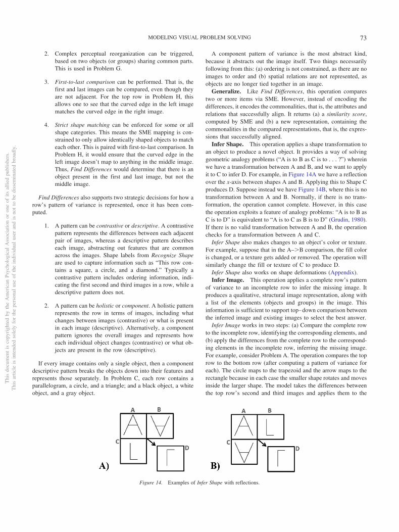
Infer Shape. This operation applies a shape transformation toan object to produce a novel object. It provides a way of solvinggeometric analogy problems (“A is to B as C is to . . . ?”) whereinwe have a transformation between A and B, and we want to applyit to C to infer D. For example, in Figure 14A we have a reflectionover the x-axis between shapes A and B. Applying this to Shape Cproduces D. Suppose instead we have Figure 14B, where this is notransformation between A and B. Normally, if there is no trans-formation, the operation cannot complete. However, in this casethe operation exploits a feature of analogy problems: “A is to B asC is to D” is equivalent to “A is to C as B is to D” (Grudin, 1980).If there is no valid transformation between A and B, the operationchecks for a transformation between A and C.

Infer Shape also makes changes to an object’s color or texture.For example, suppose that in the A–�B comparison, the fill coloris changed, or a texture gets added or removed. The operation willsimilarly change the fill or texture of C to produce D.

Infer Shape also works on shape deformations (Appendix).Infer Image. This operation applies a complete row’s pattern

of variance to an incomplete row to infer the missing image. Itproduces a qualitative, structural image representation, along witha list of the elements (objects and groups) in the image. Thisinformation is sufficient to support top–down comparison betweenthe inferred image and existing images to select the best answer.

Infer Image works in two steps: (a) Compare the complete rowto the incomplete row, identifying the corresponding elements, and(b) apply the differences from the complete row to the correspond-ing elements in the incomplete row, inferring the missing image.For example, consider Problem A. The operation compares the toprow to the bottom row (after computing a pattern of variance foreach). The circle maps to the trapezoid and the arrow maps to therectangle because in each case the smaller shape rotates and movesinside the larger shape. The model takes the differences betweenthe top row’s second and third images and applies them to the

Figure 14. Examples of Infer Shape with reflections.

Thi

sdo

cum

ent

isco

pyri

ghte

dby

the

Am

eric

anPs

ycho

logi

cal

Ass

ocia

tion

oron

eof

itsal

lied

publ

ishe

rs.

Thi

sar

ticle

isin

tend

edso

lely

for

the

pers

onal

use

ofth

ein

divi

dual

user

and

isno

tto

bedi

ssem

inat

edbr

oadl

y.


bottom row, inferring that the rectangle should rotate and be to theright of the trapezoid.

There are two ways that Infer Image can fail. First, it may beunable to apply a shape transformation. For example, there mightbe a part removal deformation, but the target object might lackextra parts to be removed. Second, the operation may find thatthere is insufficient information to compute the incomplete bottomrow’s pattern of variance. This happens on problems involvingperceptual reorganization (e.g., Problem G). Here, the model seesthat in the top row, the first and second images were both reorga-nized, suggesting that information from the third image was nec-essary to reorganize them. Because there is no third image in thebottom row, the model does not attempt to complete the operation.

Detect Texture. This operation implements the texture com-pletion strategy for nonmatrix problems (e.g., Problem I). Unlikethe other operations, it does not use HHRs—instead, it prints everyobject in an image to a bitmap and operates directly on that bitmap.Given an image, and the location of a corridor along that image(e.g., the gray rectangles in Figure 11A), it scans along the corri-dor, looking for a repeating pattern.

Additional options. Some additional options are listed below.

1. Detect Texture can be directed to insert a second imageinto the first image at a certain point. For example, it caninsert one of the answer images into the hole (the objectlabeled “Answer”) and evaluate how well that completesthe texture.

2. Detect Textures can be directed to only consider texturesat a particular frequency. After finding a repeating tex-ture at a particular frequency on the top part of Figure11A, it can be directed to seek out an answer that pro-duces a texture at the same frequency in the bottom part.

Strategic Decisions

We now consider the strategic decisions made at each step in theproblem-solving process.

1. Encoding each image. As described above, images arealways encoded at the highest level possible, Groups, meaningsimilar objects are grouped together. This ensures a sparse, simplerepresentation for problem solving.

2/3. Computing a pattern of variance for each row. If thereare fewer differences between images, then patterns of variancewill be more concise, and thus easier to store in memory. Thus,when computing a row’s pattern of variance, the model tries tominimize differences between corresponding objects. It attempts tomeet the following constraints:

A. Identicality. It’s always best if corresponding objects areidentical.

B. Relatability. If corresponding objects aren’t identical,there should be at least some valid transformation or de-formation between them.

C. Correspondence. Whenever possible, an object in oneimage should at least correspond to something in another.

If relatability is violated, the pattern of variance must describe atotal shape change. If correspondence is violated, the pattern mustdescribe an object addition. It is assumed that either of these makesthe pattern more complex and more difficult to store in memory.Below, we refer to violations of relatability or correspondence asbad object matches.

Figure 15 describes how the model pursues the above con-straints. Essentially, the model calls the Find Differences operationrepeatedly. Each call produces a pattern of variance for the row.The model evaluates the results, and if certain conditions (speci-fied in the figure) are met, it calls an updated Find Differencesoperation, specifying changes to the way images are represented orcompared.

Step I (in Figure 15) is the initial call to Find Differences. StepsII and III support basic and complex perceptual reorganization.Basic perceptual reorganization is helpful for Problem E, a figureaddition problem. Because the second image in each row is asubshape of the third image, the third image is segmented into twoobjects. These objects are identical to the first and second image,allowing the model to detect figure addition.

Complex perceptual reorganization is helpful for Problem G.Consider the top row. In the initial pattern of variance (Step I), thecorresponding objects are all different shapes. Because they con-tain similar edges, they are broken down into their edges (Step III),with each edge treated as a separate object.

Step IV checks whether there are matching objects in the firstand last images of a row. Note that Find Differences only performs

Figure 15. Steps for computing a row’s pattern of variance (each step is a call to Find Differences).

Thi

sdo

cum

ent

isco

pyri

ghte

dby

the

Am

eric

anPs

ycho

logi

cal

Ass

ocia

tion

oron

eof

itsal

lied

publ

ishe

rs.

Thi

sar

ticle

isin

tend

edso

lely

for

the

pers

onal

use

ofth

ein

divi

dual

user

and

isno

tto

bedi

ssem

inat

edbr

oadl

y.


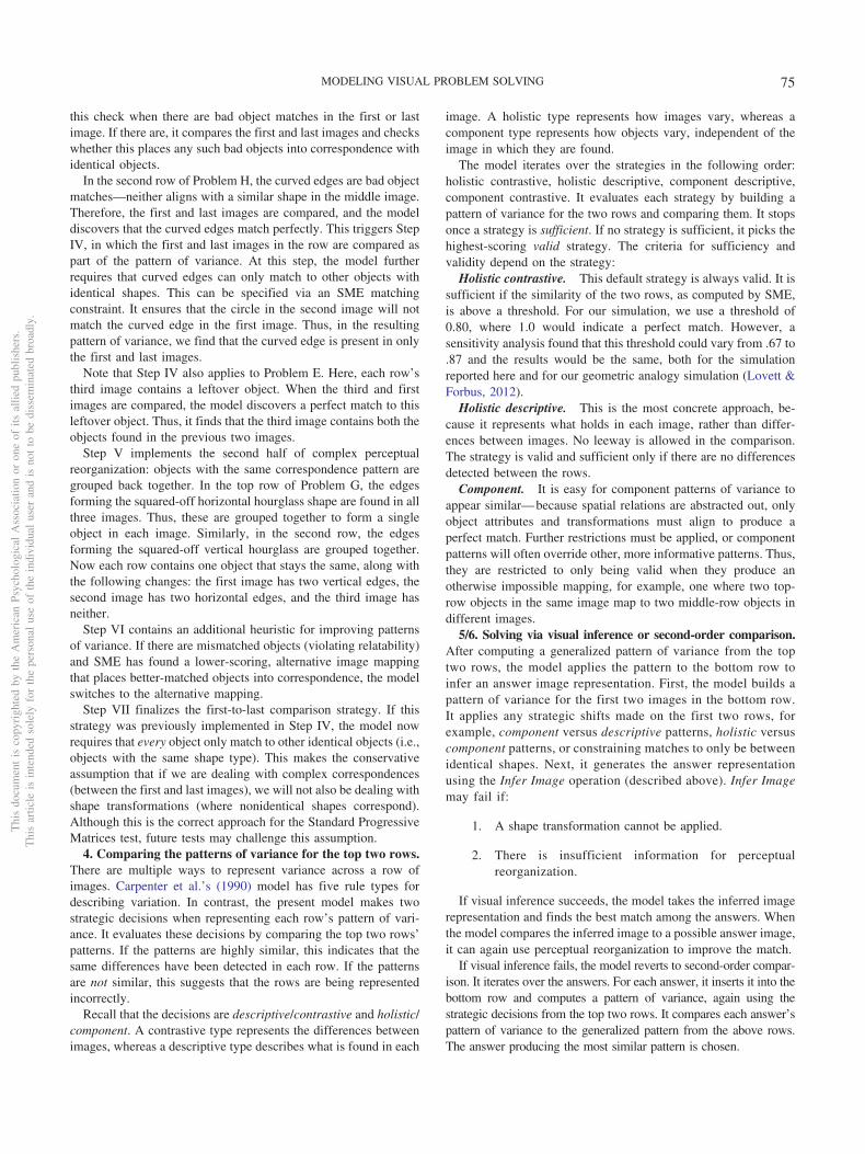
this check when there are bad object matches in the first or lastimage. If there are, it compares the first and last images and checkswhether this places any such bad objects into correspondence withidentical objects.

In the second row of Problem H, the curved edges are bad objectmatches—neither aligns with a similar shape in the middle image.Therefore, the first and last images are compared, and the modeldiscovers that the curved edges match perfectly. This triggers StepIV, in which the first and last images in the row are compared aspart of the pattern of variance. At this step, the model furtherrequires that curved edges can only match to other objects withidentical shapes. This can be specified via an SME matchingconstraint. It ensures that the circle in the second image will notmatch the curved edge in the first image. Thus, in the resultingpattern of variance, we find that the curved edge is present in onlythe first and last images.

Note that Step IV also applies to Problem E. Here, each row’sthird image contains a leftover object. When the third and firstimages are compared, the model discovers a perfect match to thisleftover object. Thus, it finds that the third image contains both theobjects found in the previous two images.

Step V implements the second half of complex perceptualreorganization: objects with the same correspondence pattern aregrouped back together. In the top row of Problem G, the edgesforming the squared-off horizontal hourglass shape are found in allthree images. Thus, these are grouped together to form a singleobject in each image. Similarly, in the second row, the edgesforming the squared-off vertical hourglass are grouped together.Now each row contains one object that stays the same, along withthe following changes: the first image has two vertical edges, thesecond image has two horizontal edges, and the third image hasneither.

Step VI contains an additional heuristic for improving patternsof variance. If there are mismatched objects (violating relatability)and SME has found a lower-scoring, alternative image mappingthat places better-matched objects into correspondence, the modelswitches to the alternative mapping.

Step VII finalizes the first-to-last comparison strategy. If thisstrategy was previously implemented in Step IV, the model nowrequires that every object only match to other identical objects (i.e.,objects with the same shape type). This makes the conservativeassumption that if we are dealing with complex correspondences(between the first and last images), we will not also be dealing withshape transformations (where nonidentical shapes correspond).Although this is the correct approach for the Standard ProgressiveMatrices test, future tests may challenge this assumption.

4. Comparing the patterns of variance for the top two rows.There are multiple ways to represent variance across a row ofimages. Carpenter et al.’s (1990) model has five rule types fordescribing variation. In contrast, the present model makes twostrategic decisions when representing each row’s pattern of vari-ance. It evaluates these decisions by comparing the top two rows’patterns. If the patterns are highly similar, this indicates that thesame differences have been detected in each row. If the patternsare not similar, this suggests that the rows are being representedincorrectly.

Recall that the decisions are descriptive/contrastive and holistic/component. A contrastive type represents the differences betweenimages, whereas a descriptive type describes what is found in each

image. A holistic type represents how images vary, whereas acomponent type represents how objects vary, independent of theimage in which they are found.

The model iterates over the strategies in the following order:holistic contrastive, holistic descriptive, component descriptive,component contrastive. It evaluates each strategy by building apattern of variance for the two rows and comparing them. It stopsonce a strategy is sufficient. If no strategy is sufficient, it picks thehighest-scoring valid strategy. The criteria for sufficiency andvalidity depend on the strategy:

Holistic contrastive. This default strategy is always valid. It issufficient if the similarity of the two rows, as computed by SME,is above a threshold. For our simulation, we use a threshold of0.80, where 1.0 would indicate a perfect match. However, asensitivity analysis found that this threshold could vary from .67 to.87 and the results would be the same, both for the simulationreported here and for our geometric analogy simulation (Lovett &Forbus, 2012).

Holistic descriptive. This is the most concrete approach, be-cause it represents what holds in each image, rather than differ-ences between images. No leeway is allowed in the comparison.The strategy is valid and sufficient only if there are no differencesdetected between the rows.

Component. It is easy for component patterns of variance toappear similar—because spatial relations are abstracted out, onlyobject attributes and transformations must align to produce aperfect match. Further restrictions must be applied, or componentpatterns will often override other, more informative patterns. Thus,they are restricted to only being valid when they produce anotherwise impossible mapping, for example, one where two top-row objects in the same image map to two middle-row objects indifferent images.

5/6. Solving via visual inference or second-order comparison.After computing a generalized pattern of variance from the toptwo rows, the model applies the pattern to the bottom row toinfer an answer image representation. First, the model builds apattern of variance for the first two images in the bottom row.It applies any strategic shifts made on the first two rows, forexample, component versus descriptive patterns, holistic versuscomponent patterns, or constraining matches to only be betweenidentical shapes. Next, it generates the answer representationusing the Infer Image operation (described above). Infer Imagemay fail if:

1. A shape transformation cannot be applied.

2. There is insufficient information for perceptualreorganization.

If visual inference succeeds, the model takes the inferred imagerepresentation and finds the best match among the answers. Whenthe model compares the inferred image to a possible answer image,it can again use perceptual reorganization to improve the match.

If visual inference fails, the model reverts to second-order compar-ison. It iterates over the answers. For each answer, it inserts it into thebottom row and computes a pattern of variance, again using thestrategic decisions from the top two rows. It compares each answer’spattern of variance to the generalized pattern from the above rows.The answer producing the most similar pattern is chosen.

Thi

sdo

cum

ent

isco

pyri

ghte

dby

the

Am

eric

anPs

ycho

logi

cal

Ass

ocia

tion

oron

eof

itsal

lied

publ

ishe

rs.

Thi

sar

ticle

isin

tend

edso

lely

for

the

pers

onal

use

ofth

ein

divi

dual

user

and

isno

tto

bedi

ssem

inat

edbr

oadl

y.


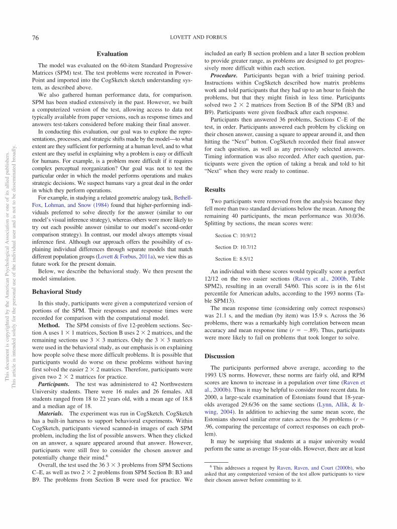
Evaluation

The model was evaluated on the 60-item Standard ProgressiveMatrices (SPM) test. The test problems were recreated in Power-Point and imported into the CogSketch sketch understanding sys-tem, as described above.

We also gathered human performance data, for comparison.SPM has been studied extensively in the past. However, we builta computerized version of the test, allowing access to data nottypically available from paper versions, such as response times andanswers test-takers considered before making their final answer.

In conducting this evaluation, our goal was to explore the repre-sentations, processes, and strategic shifts made by the model—to whatextent are they sufficient for performing at a human level, and to whatextent are they useful in explaining why a problem is easy or difficultfor humans. For example, is a problem more difficult if it requirescomplex perceptual reorganization? Our goal was not to test theparticular order in which the model performs operations and makesstrategic decisions. We suspect humans vary a great deal in the orderin which they perform operations.

For example, in studying a related geometric analogy task, Bethell-Fox, Lohman, and Snow (1984) found that higher-performing indi-viduals preferred to solve directly for the answer (similar to ourmodel’s visual inference strategy), whereas others were more likely totry out each possible answer (similar to our model’s second-ordercomparison strategy). In contrast, our model always attempts visualinference first. Although our approach offers the possibility of ex-plaining individual differences through separate models that matchdifferent population groups (Lovett & Forbus, 2011a), we view this asfuture work for the present domain.

Below, we describe the behavioral study. We then present themodel simulation.

Behavioral Study

In this study, participants were given a computerized version ofportions of the SPM. Their responses and response times wererecorded for comparison with the computational model.

Method. The SPM consists of five 12-problem sections. Sec-tion A uses 1 � 1 matrices, Section B uses 2 � 2 matrices, and theremaining sections use 3 � 3 matrices. Only the 3 � 3 matriceswere used in the behavioral study, as our emphasis is on explaininghow people solve these more difficult problems. It is possible thatparticipants would do worse on these problems without havingfirst solved the easier 2 � 2 matrices. Therefore, participants weregiven two 2 � 2 matrices for practice.

Participants. The test was administered to 42 NorthwesternUniversity students. There were 16 males and 26 females. Allstudents ranged from 18 to 22 years old, with a mean age of 18.8and a median age of 18.

Materials. The experiment was run in CogSketch. CogSketchhas a built-in harness to support behavioral experiments. WithinCogSketch, participants viewed scanned-in images of each SPMproblem, including the list of possible answers. When they clickedon an answer, a square appeared around that answer. However,participants were still free to consider the chosen answer andpotentially change their mind.6

Overall, the test used the 36 3 � 3 problems from SPM SectionsC–E, as well as two 2 � 2 problems from SPM Section B: B3 andB9. The problems from Section B were used for practice. We

included an early B section problem and a later B section problemto provide greater range, as problems are designed to get progres-sively more difficult within each section.

Procedure. Participants began with a brief training period.Instructions within CogSketch described how matrix problemswork and told participants that they had up to an hour to finish theproblems, but that they might finish in less time. Participantssolved two 2 � 2 matrices from Section B of the SPM (B3 andB9). Participants were given feedback after each response.

Participants then answered 36 problems, Sections C–E of thetest, in order. Participants answered each problem by clicking ontheir chosen answer, causing a square to appear around it, and thenhitting the “Next” button. CogSketch recorded their final answerfor each question, as well as any previously selected answers.Timing information was also recorded. After each question, par-ticipants were given the option of taking a break and told to hit“Next” when they were ready to continue.

Results

Two participants were removed from the analysis because theyfell more than two standard deviations below the mean. Among theremaining 40 participants, the mean performance was 30.0/36.Splitting by sections, the mean scores were:

Section C: 10.9/12

Section D: 10.7/12

Section E: 8.5/12

An individual with these scores would typically score a perfect12/12 on the two easier sections (Raven et al., 2000b, TableSPM2), resulting in an overall 54/60. This score is in the 61stpercentile for American adults, according to the 1993 norms (Ta-ble SPM13).

The mean response time (considering only correct responses)was 21.1 s, and the median (by item) was 15.9 s. Across the 36problems, there was a remarkably high correlation between meanaccuracy and mean response time (r � �.89). Thus, participantswere more likely to fail on problems that took longer to solve.

Discussion

The participants performed above average, according to the1993 US norms. However, these norms are fairly old, and RPMscores are known to increase in a population over time (Raven etal., 2000b). Thus it may be helpful to consider more recent data. In2000, a large-scale examination of Estonians found that 18-year-olds averaged 29.6/36 on the same sections (Lynn, Allik, & Ir-wing, 2004). In addition to achieving the same mean score, theEstonians showed similar error rates across the 36 problems (r �.96, comparing the percentage of correct responses on each prob-lem).

It may be surprising that students at a major university wouldperform the same as average 18-year-olds. However, there are at least

6 This addresses a request by Raven, Raven, and Court (2000b), whoasked that any computerized version of the test allow participants to viewtheir chosen answer before committing to it.

Thi

sdo

cum

ent

isco

pyri

ghte

dby

the

Am

eric

anPs

ycho

logi

cal

Ass

ocia

tion

oron

eof

itsal

lied

publ

ishe

rs.

Thi

sar

ticle

isin

tend

edso

lely

for

the

pers

onal

use

ofth

ein

divi

dual

user

and

isno

tto

bedi

ssem

inat

edbr

oadl

y.


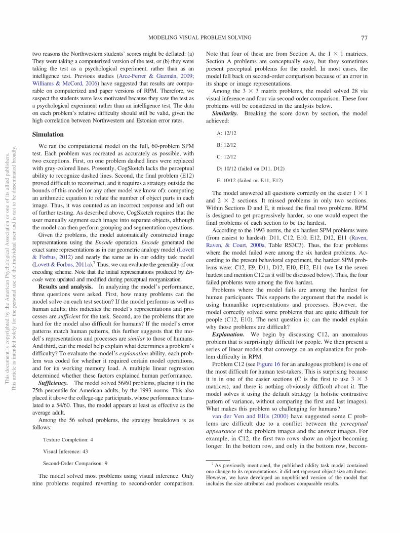
two reasons the Northwestern students’ scores might be deflated: (a)They were taking a computerized version of the test, or (b) they weretaking the test as a psychological experiment, rather than as anintelligence test. Previous studies (Arce-Ferrer & Guzmán, 2009;Williams & McCord, 2006) have suggested that results are compa-rable on computerized and paper versions of RPM. Therefore, wesuspect the students were less motivated because they saw the test asa psychological experiment rather than an intelligence test. The dataon each problem’s relative difficulty should still be valid, given thehigh correlation between Northwestern and Estonian error rates.

Simulation

We ran the computational model on the full, 60-problem SPMtest. Each problem was recreated as accurately as possible, withtwo exceptions. First, on one problem dashed lines were replacedwith gray-colored lines. Presently, CogSketch lacks the perceptualability to recognize dashed lines. Second, the final problem (E12)proved difficult to reconstruct, and it requires a strategy outside thebounds of this model (or any other model we know of): computingan arithmetic equation to relate the number of object parts in eachimage. Thus, it was counted as an incorrect response and left outof further testing. As described above, CogSketch requires that theuser manually segment each image into separate objects, althoughthe model can then perform grouping and segmentation operations.

Given the problems, the model automatically constructed imagerepresentations using the Encode operation. Encode generated theexact same representations as in our geometric analogy model (Lovett& Forbus, 2012) and nearly the same as in our oddity task model(Lovett & Forbus, 2011a).7 Thus, we can evaluate the generality of ourencoding scheme. Note that the initial representations produced by En-code were updated and modified during perceptual reorganization.

Results and analysis. In analyzing the model’s performance,three questions were asked. First, how many problems can themodel solve on each test section? If the model performs as well ashuman adults, this indicates the model’s representations and pro-cesses are sufficient for the task. Second, are the problems that arehard for the model also difficult for humans? If the model’s errorpatterns match human patterns, this further suggests that the mo-del’s representations and processes are similar to those of humans.And third, can the model help explain what determines a problem’sdifficulty? To evaluate the model’s explanation ability, each prob-lem was coded for whether it required certain model operations,and for its working memory load. A multiple linear regressiondetermined whether these factors explained human performance.

Sufficiency. The model solved 56/60 problems, placing it in the75th percentile for American adults, by the 1993 norms. This alsoplaced it above the college-age participants, whose performance trans-lated to a 54/60. Thus, the model appears at least as effective as theaverage adult.

Among the 56 solved problems, the strategy breakdown is asfollows:

Texture Completion: 4

Visual Inference: 43

Second-Order Comparison: 9

The model solved most problems using visual inference. Onlynine problems required reverting to second-order comparison.

Note that four of these are from Section A, the 1 � 1 matrices.Section A problems are conceptually easy, but they sometimespresent perceptual problems for the model. In most cases, themodel fell back on second-order comparison because of an error inits shape or image representations.

Among the 3 � 3 matrix problems, the model solved 28 viavisual inference and four via second-order comparison. These fourproblems will be considered in the analysis below.

Similarity. Breaking the score down by section, the modelachieved:

A: 12/12

B: 12/12

C: 12/12

D: 10/12 (failed on D11, D12)

E: 10/12 (failed on E11, E12)

The model answered all questions correctly on the easier 1 � 1and 2 � 2 sections. It missed problems in only two sections.Within Sections D and E, it missed the final two problems. RPMis designed to get progressively harder, so one would expect thefinal problems of each section to be the hardest.

According to the 1993 norms, the six hardest SPM problems were(from easiest to hardest): D11, C12, E10, E12, D12, E11 (Raven,Raven, & Court, 2000a, Table RS3C3). Thus, the four problemswhere the model failed were among the six hardest problems. Ac-cording to the present behavioral experiment, the hardest SPM prob-lems were: C12, E9, D11, D12, E10, E12, E11 (we list the sevenhardest and mention C12 as it will be discussed below). Thus, the fourfailed problems were among the five hardest.

Problems where the model fails are among the hardest forhuman participants. This supports the argument that the model isusing humanlike representations and processes. However, themodel correctly solved some problems that are quite difficult forpeople (C12, E10). The next question is: can the model explainwhy those problems are difficult?

Explanation. We begin by discussing C12, an anomalousproblem that is surprisingly difficult for people. We then present aseries of linear models that converge on an explanation for prob-lem difficulty in RPM.

Problem C12 (see Figure 16 for an analogous problem) is one ofthe most difficult for human test-takers. This is surprising becauseit is in one of the easier sections (C is the first to use 3 � 3matrices), and there is nothing obviously difficult about it. Themodel solves it using the default strategy (a holistic contrastivepattern of variance, without comparing the first and last images).What makes this problem so challenging for humans?

van der Ven and Ellis (2000) have suggested some C prob-lems are difficult due to a conflict between the perceptualappearance of the problem images and the answer images. Forexample, in C12, the first two rows show an object becominglonger. In the bottom row, and only in the bottom row, becom-

7 As previously mentioned, the published oddity task model containedone change to its representations: it did not represent object size attributes.However, we have developed an unpublished version of the model thatincludes the size attributes and produces comparable results.

Thi

sdo

cum

ent

isco

pyri

ghte

dby

the

Am

eric

anPs

ycho

logi

cal

Ass

ocia

tion

oron

eof

itsal

lied

publ

ishe

rs.

Thi

sar

ticle

isin

tend

edso

lely

for

the

pers

onal

use

ofth

ein

divi

dual

user

and

isno

tto

bedi

ssem

inat

edbr

oadl

y.


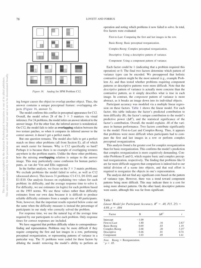
ing longer causes the object to overlap another object. Thus, theanswer contains a unique perceptual feature: overlapping ob-jects (Figure 16, answer 3).

The model confirms this conflict in perceptual appearance for C12.Overall, the model solves 28 of the 3 � 3 matrices via visualinference. For 24 problems, the model infers an answer identical to theanswer image. For the other four, the inferred answer is nonidentical.On C12, the model fails to infer an overlapping relation between thetwo texture patches, so when it compares its inferred answer to thecorrect answer, it doesn’t get a perfect match.

But one question remains. The model also fails to get a perfectmatch on three other problems (all from Section E), all of whichare much easier for humans. Why is C12 specifically so hard?Perhaps it is because there is no example of overlapping texturesanywhere in the problem matrix. Unlike the three other problems,here the missing overlapping relation is unique to the answerimage. This may particularly cause confusion for human partici-pants, as van der Ven and Ellis supposed.

In the further analysis, we focus on the 3 � 3 matrix problems.We exclude problems the model failed to solve, as well as C12(discussed above). This leaves 31 problems: C1-C11, D1-D10, andE1-E10. Our analysis focuses on explaining two values for eachproblem: its difficulty, and the average response time to solve it.For difficulty, we use estimates (in logits) for each problem basedon the 1993 norms. We use these values rather than difficultyestimates from our own data because it is difficult to producereliable difficulty estimates from a sample size of 40 participants.Note, however, that the important results reported below come outthe same when the difficulty measure is instead the percentage ofparticipants in our study who correctly solved the problem.

For response time, we use the natural log of the average timerequired by our participants to solve each problem. Only responsetimes for correct responses are included.

We have suggested that problem difficulty relates to correspondence-finding and representation. Problems may be more difficult if theyrequire comparing the first and last images in a row, performingperceptual reorganization, or representing patterns of variance in aparticular way. The 31 problems were coded for these factors byablating the model: removing the model’s ability to perform an

operation and noting which problems it now failed to solve. In total,five factors were evaluated:

First-to-Last: Comparing the first and last images in the row.

Basic-Reorg: Basic perceptual reorganization.

Complex-Reorg: Complex perceptual reorganization.

Descriptive: Using a descriptive pattern of variance.

Component: Using a component pattern of variance.

Each factor could be 1 (indicating that a problem required thisoperation) or 0. The final two factors determine which pattern ofvariance types can be encoded. We presupposed that holisticcontrastive pattern might be the most natural (e.g., example Prob-lem A), and thus tested whether problems requiring componentpatterns or descriptive patterns were more difficult. Note that thedescriptive pattern of variance is actually more concrete than thecontrastive pattern, as it simply describes what is true in eachimage. In contrast, the component pattern of variance is moreabstract, as it breaks an image down into its individual objects.

Participant accuracy was modeled via a multiple linear regres-sion on these factors. Table 1 shows the linear model. For eachfactor, this table indicates the factor’s predicted contribution toitem difficulty (B), the factor’s unique contribution to the model’spredictive power (�R2), and the statistical significance of thefactor’s contribution. Overall, the model explains .48 of the vari-ance in human performance. Two factors contribute significantlyto the model: First-to-Last and Complex-Reorg. Thus, it appearsthat problems were more difficult when participants had to com-pare the first and last images in a row or perform complexperceptual reorganization.

This analysis found a far greater cost for complex reorganizationthan for basic reorganization. This confirms the model’s predictionthat complex reorganization is more cognitively demanding. Con-sider Problems E and G, which require basic and complex percep-tual reorganization, respectively. The finding that problems like Gare far more difficult suggests that comparison is indeed tied to ourinitial division of a scene into objects, and that real effort isrequired to reorganize the objects in one’s representation.

The analysis did not find any significant costs based on the patternof variance type. However, there was a trend toward componentpatterns being more difficult. This may indicate there is a cost forusing more abstract patterns. On the other hand, descriptive patternswere easier, although this was far from significant.

Table 1Linear Model for Participant Accuracy, R2 � .48, F(5, 25) �4.69, p � .004

Factor B �R2 t

Intercept �1.09First-to-Last 1.80 .16 2.83�

Basic-Reorg 0.69 .03 1.19Complex-Reorg 2.68 .20 3.15�

Descriptive �0.46 .01 0.74Component 1.03 .05 1.61

Note. Reorg � Reorganization.� p � .05.

Figure 16. Analog for SPM Problem C12.

Thi

sdo

cum

ent

isco

pyri

ghte

dby

the

Am

eric

anPs

ycho

logi

cal

Ass

ocia

tion

oron

eof

itsal

lied

publ

ishe

rs.

Thi

sar

ticle

isin

tend

edso

lely

for

the

pers

onal

use

ofth

ein

divi

dual

user

and

isno

tto

bedi

ssem

inat

edbr

oadl

y.


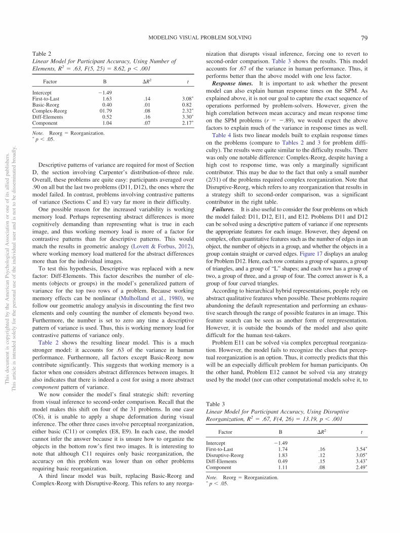
Descriptive patterns of variance are required for most of SectionD, the section involving Carpenter’s distribution-of-three rule.Overall, these problems are quite easy: participants averaged over.90 on all but the last two problems (D11, D12), the ones where themodel failed. In contrast, problems involving contrastive patternsof variance (Sections C and E) vary far more in their difficulty.

One possible reason for the increased variability is workingmemory load. Perhaps representing abstract differences is morecognitively demanding than representing what is true in eachimage, and thus working memory load is more of a factor forcontrastive patterns than for descriptive patterns. This wouldmatch the results in geometric analogy (Lovett & Forbus, 2012),where working memory load mattered for the abstract differencesmore than for the individual images.

To test this hypothesis, Descriptive was replaced with a newfactor: Diff-Elements. This factor describes the number of ele-ments (objects or groups) in the model’s generalized pattern ofvariance for the top two rows of a problem. Because workingmemory effects can be nonlinear (Mulholland et al., 1980), wefollow our geometric analogy analysis in discounting the first twoelements and only counting the number of elements beyond two.Furthermore, the number is set to zero any time a descriptivepattern of variance is used. Thus, this is working memory load forcontrastive patterns of variance only.

Table 2 shows the resulting linear model. This is a muchstronger model: it accounts for .63 of the variance in humanperformance. Furthermore, all factors except Basic-Reorg nowcontribute significantly. This suggests that working memory is afactor when one considers abstract differences between images. Italso indicates that there is indeed a cost for using a more abstractcomponent pattern of variance.

We now consider the model’s final strategic shift: revertingfrom visual inference to second-order comparison. Recall that themodel makes this shift on four of the 31 problems. In one case(C6), it is unable to apply a shape deformation during visualinference. The other three cases involve perceptual reorganization,either basic (C11) or complex (E8, E9). In each case, the modelcannot infer the answer because it is unsure how to organize theobjects in the bottom row’s first two images. It is interesting tonote that although C11 requires only basic reorganization, theaccuracy on this problem was lower than on other problemsrequiring basic reorganization.

A third linear model was built, replacing Basic-Reorg andComplex-Reorg with Disruptive-Reorg. This refers to any reorga-

nization that disrupts visual inference, forcing one to revert tosecond-order comparison. Table 3 shows the results. This modelaccounts for .67 of the variance in human performance. Thus, itperforms better than the above model with one less factor.

Response times. It is important to ask whether the presentmodel can also explain human response times on the SPM. Asexplained above, it is not our goal to capture the exact sequence ofoperations performed by problem-solvers. However, given thehigh correlation between mean accuracy and mean response timeon the SPM problems (r � �.89), we would expect the abovefactors to explain much of the variance in response times as well.

Table 4 lists two linear models built to explain response timeson the problems (compare to Tables 2 and 3 for problem diffi-culty). The results were quite similar to the difficulty results. Therewas only one notable difference: Complex-Reorg, despite having ahigh cost to response time, was only a marginally significantcontributor. This may be due to the fact that only a small number(2/31) of the problems required complex reorganization. Note thatDisruptive-Reorg, which refers to any reorganization that results ina strategy shift to second-order comparison, was a significantcontributor in the right table.

Failures. It is also useful to consider the four problems on whichthe model failed: D11, D12, E11, and E12. Problems D11 and D12can be solved using a descriptive pattern of variance if one representsthe appropriate features for each image. However, they depend oncomplex, often quantitative features such as the number of edges in anobject, the number of objects in a group, and whether the objects in agroup contain straight or curved edges. Figure 17 displays an analogfor Problem D12. Here, each row contains a group of squares, a groupof triangles, and a group of “L” shapes; and each row has a group oftwo, a group of three, and a group of four. The correct answer is 8, agroup of four curved triangles.

According to hierarchical hybrid representations, people rely onabstract qualitative features when possible. These problems requireabandoning the default representation and performing an exhaus-tive search through the range of possible features in an image. Thisfeature search can be seen as another form of rerepresentation.However, it is outside the bounds of the model and also quitedifficult for the human test-takers.

Problem E11 can be solved via complex perceptual reorganiza-tion. However, the model fails to recognize the clues that percep-tual reorganization is an option. Thus, it correctly predicts that thiswill be an especially difficult problem for human participants. Onthe other hand, Problem E12 cannot be solved via any strategyused by the model (nor can other computational models solve it, to

Table 2Linear Model for Participant Accuracy, Using Number ofElements, R2 � .63, F(5, 25) � 8.62, p � .001

Factor B �R2 t


Basic-Reorg 0.40 .01 0.82Complex-Reorg 01.79 .08 2.32�

Diff-Elements 0.52 .16 3.30�

Component 1.04 .07 2.17�


Table 3Linear Model for Participant Accuracy, Using DisruptiveReorganization, R2 � .67, F(4, 26) � 13.19, p � .001

Factor B �R2 t


Disruptive-Reorg 1.83 .12 3.05�


Component 1.11 .08 2.49�


Thi

sdo

cum

ent

isco

pyri

ghte

dby

the

Am

eric

anPs

ycho

logi

cal

Ass

ocia

tion

oron

eof

itsal

lied

publ

ishe

rs.

Thi

sar

ticle

isin

tend

edso

lely

for

the

pers

onal

use

ofth

ein

divi

dual

user

and

isno

tto

bedi

ssem

inat

edbr

oadl

y.


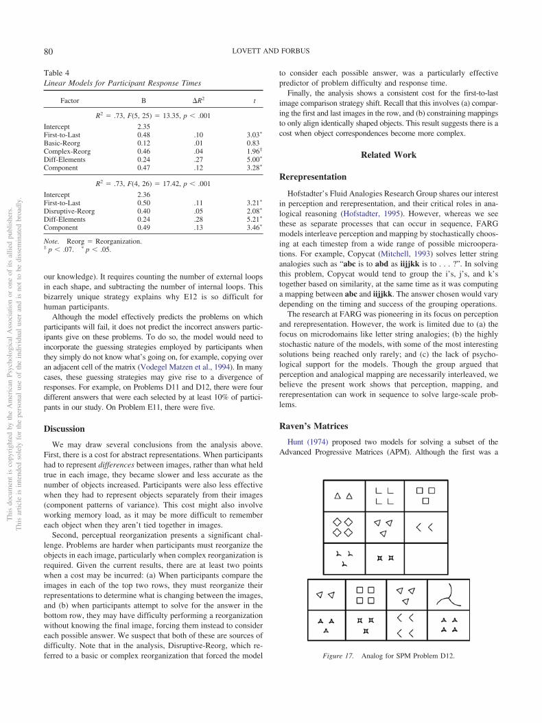
our knowledge). It requires counting the number of external loopsin each shape, and subtracting the number of internal loops. Thisbizarrely unique strategy explains why E12 is so difficult forhuman participants.

Although the model effectively predicts the problems on whichparticipants will fail, it does not predict the incorrect answers partic-ipants give on these problems. To do so, the model would need toincorporate the guessing strategies employed by participants whenthey simply do not know what’s going on, for example, copying overan adjacent cell of the matrix (Vodegel Matzen et al., 1994). In manycases, these guessing strategies may give rise to a divergence ofresponses. For example, on Problems D11 and D12, there were fourdifferent answers that were each selected by at least 10% of partici-pants in our study. On Problem E11, there were five.

Discussion

We may draw several conclusions from the analysis above.First, there is a cost for abstract representations. When participantshad to represent differences between images, rather than what heldtrue in each image, they became slower and less accurate as thenumber of objects increased. Participants were also less effectivewhen they had to represent objects separately from their images(component patterns of variance). This cost might also involveworking memory load, as it may be more difficult to remembereach object when they aren’t tied together in images.

Second, perceptual reorganization presents a significant chal-lenge. Problems are harder when participants must reorganize theobjects in each image, particularly when complex reorganization isrequired. Given the current results, there are at least two pointswhen a cost may be incurred: (a) When participants compare theimages in each of the top two rows, they must reorganize theirrepresentations to determine what is changing between the images,and (b) when participants attempt to solve for the answer in thebottom row, they may have difficulty performing a reorganizationwithout knowing the final image, forcing them instead to considereach possible answer. We suspect that both of these are sources ofdifficulty. Note that in the analysis, Disruptive-Reorg, which re-ferred to a basic or complex reorganization that forced the model

to consider each possible answer, was a particularly effectivepredictor of problem difficulty and response time.

Finally, the analysis shows a consistent cost for the first-to-lastimage comparison strategy shift. Recall that this involves (a) compar-ing the first and last images in the row, and (b) constraining mappingsto only align identically shaped objects. This result suggests there is acost when object correspondences become more complex.

Related Work

Rerepresentation

Hofstadter’s Fluid Analogies Research Group shares our interestin perception and rerepresentation, and their critical roles in ana-logical reasoning (Hofstadter, 1995). However, whereas we seethese as separate processes that can occur in sequence, FARGmodels interleave perception and mapping by stochastically choos-ing at each timestep from a wide range of possible microopera-tions. For example, Copycat (Mitchell, 1993) solves letter stringanalogies such as “abc is to abd as iijjkk is to . . . ?”. In solvingthis problem, Copycat would tend to group the i’s, j’s, and k’stogether based on similarity, at the same time as it was computinga mapping between abc and iijjkk. The answer chosen would varydepending on the timing and success of the grouping operations.

The research at FARG was pioneering in its focus on perceptionand rerepresentation. However, the work is limited due to (a) thefocus on microdomains like letter string analogies; (b) the highlystochastic nature of the models, with some of the most interestingsolutions being reached only rarely; and (c) the lack of psycho-logical support for the models. Though the group argued thatperception and analogical mapping are necessarily interleaved, webelieve the present work shows that perception, mapping, andrerepresentation can work in sequence to solve large-scale prob-lems.

Raven’s Matrices

Hunt (1974) proposed two models for solving a subset of theAdvanced Progressive Matrices (APM). Although the first was a

Figure 17. Analog for SPM Problem D12.

Table 4Linear Models for Participant Response Times

Factor B �R2 t

R2 � .73, F(5, 25) � 13.35, p � .001

Intercept 2.35First-to-Last 0.48 .10 3.03�

Basic-Reorg 0.12 .01 0.83Complex-Reorg 0.46 .04 1.96‡


Component 0.47 .12 3.28�

R2 � .73, F(4, 26) � 17.42, p � .001

Intercept 2.36First-to-Last 0.50 .11 3.21�

Disruptive-Reorg 0.40 .05 2.08�


Component 0.49 .13 3.46�

Note. Reorg � Reorganization.‡ p � .07. � p � .05.

Thi

sdo

cum

ent

isco

pyri

ghte

dby

the

Am

eric

anPs

ycho

logi

cal

Ass

ocia

tion

oron

eof

itsal

lied

publ

ishe

rs.

Thi

sar

ticle

isin

tend

edso

lely

for

the

pers

onal

use

ofth

ein

divi

dual

user

and

isno

tto

bedi

ssem

inat

edbr

oadl

y.


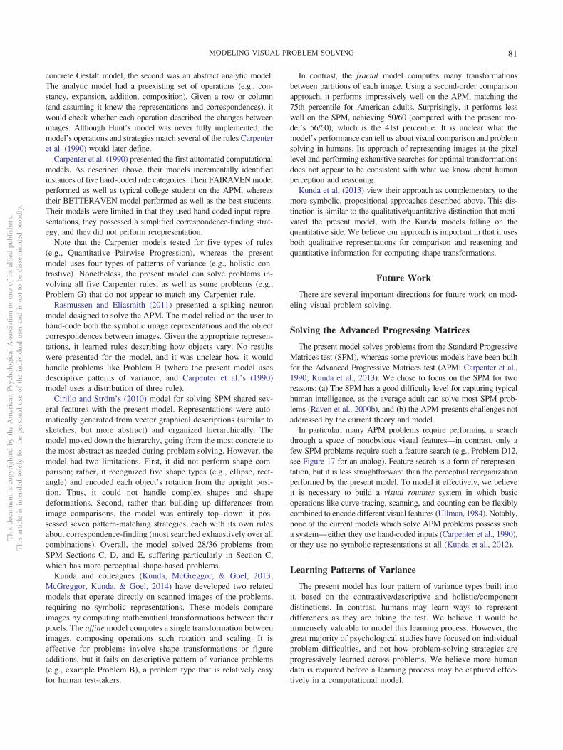
concrete Gestalt model, the second was an abstract analytic model.The analytic model had a preexisting set of operations (e.g., con-stancy, expansion, addition, composition). Given a row or column(and assuming it knew the representations and correspondences), itwould check whether each operation described the changes betweenimages. Although Hunt’s model was never fully implemented, themodel’s operations and strategies match several of the rules Carpenteret al. (1990) would later define.

Carpenter et al. (1990) presented the first automated computationalmodels. As described above, their models incrementally identifiedinstances of five hard-coded rule categories. Their FAIRAVEN modelperformed as well as typical college student on the APM, whereastheir BETTERAVEN model performed as well as the best students.Their models were limited in that they used hand-coded input repre-sentations, they possessed a simplified correspondence-finding strat-egy, and they did not perform rerepresentation.

Note that the Carpenter models tested for five types of rules(e.g., Quantitative Pairwise Progression), whereas the presentmodel uses four types of patterns of variance (e.g., holistic con-trastive). Nonetheless, the present model can solve problems in-volving all five Carpenter rules, as well as some problems (e.g.,Problem G) that do not appear to match any Carpenter rule.

Rasmussen and Eliasmith (2011) presented a spiking neuronmodel designed to solve the APM. The model relied on the user tohand-code both the symbolic image representations and the objectcorrespondences between images. Given the appropriate represen-tations, it learned rules describing how objects vary. No resultswere presented for the model, and it was unclear how it wouldhandle problems like Problem B (where the present model usesdescriptive patterns of variance, and Carpenter et al.’s (1990)model uses a distribution of three rule).

Cirillo and Ström’s (2010) model for solving SPM shared sev-eral features with the present model. Representations were auto-matically generated from vector graphical descriptions (similar tosketches, but more abstract) and organized hierarchically. Themodel moved down the hierarchy, going from the most concrete tothe most abstract as needed during problem solving. However, themodel had two limitations. First, it did not perform shape com-parison; rather, it recognized five shape types (e.g., ellipse, rect-angle) and encoded each object’s rotation from the upright posi-tion. Thus, it could not handle complex shapes and shapedeformations. Second, rather than building up differences fromimage comparisons, the model was entirely top–down: it pos-sessed seven pattern-matching strategies, each with its own rulesabout correspondence-finding (most searched exhaustively over allcombinations). Overall, the model solved 28/36 problems fromSPM Sections C, D, and E, suffering particularly in Section C,which has more perceptual shape-based problems.

Kunda and colleagues (Kunda, McGreggor, & Goel, 2013;McGreggor, Kunda, & Goel, 2014) have developed two relatedmodels that operate directly on scanned images of the problems,requiring no symbolic representations. These models compareimages by computing mathematical transformations between theirpixels. The affine model computes a single transformation betweenimages, composing operations such rotation and scaling. It iseffective for problems involve shape transformations or figureadditions, but it fails on descriptive pattern of variance problems(e.g., example Problem B), a problem type that is relatively easyfor human test-takers.

In contrast, the fractal model computes many transformationsbetween partitions of each image. Using a second-order comparisonapproach, it performs impressively well on the APM, matching the75th percentile for American adults. Surprisingly, it performs lesswell on the SPM, achieving 50/60 (compared with the present mo-del’s 56/60), which is the 41st percentile. It is unclear what themodel’s performance can tell us about visual comparison and problemsolving in humans. Its approach of representing images at the pixellevel and performing exhaustive searches for optimal transformationsdoes not appear to be consistent with what we know about humanperception and reasoning.

Kunda et al. (2013) view their approach as complementary to themore symbolic, propositional approaches described above. This dis-tinction is similar to the qualitative/quantitative distinction that moti-vated the present model, with the Kunda models falling on thequantitative side. We believe our approach is important in that it usesboth qualitative representations for comparison and reasoning andquantitative information for computing shape transformations.

Future Work

There are several important directions for future work on mod-eling visual problem solving.

Solving the Advanced Progressing Matrices

The present model solves problems from the Standard ProgressiveMatrices test (SPM), whereas some previous models have been builtfor the Advanced Progressive Matrices test (APM; Carpenter et al.,1990; Kunda et al., 2013). We chose to focus on the SPM for tworeasons: (a) The SPM has a good difficulty level for capturing typicalhuman intelligence, as the average adult can solve most SPM prob-lems (Raven et al., 2000b), and (b) the APM presents challenges notaddressed by the current theory and model.

In particular, many APM problems require performing a searchthrough a space of nonobvious visual features—in contrast, only afew SPM problems require such a feature search (e.g., Problem D12,see Figure 17 for an analog). Feature search is a form of rerepresen-tation, but it is less straightforward than the perceptual reorganizationperformed by the present model. To model it effectively, we believeit is necessary to build a visual routines system in which basicoperations like curve-tracing, scanning, and counting can be flexiblycombined to encode different visual features (Ullman, 1984). Notably,none of the current models which solve APM problems possess sucha system—either they use hand-coded inputs (Carpenter et al., 1990),or they use no symbolic representations at all (Kunda et al., 2012).

Learning Patterns of Variance

The present model has four pattern of variance types built intoit, based on the contrastive/descriptive and holistic/componentdistinctions. In contrast, humans may learn ways to representdifferences as they are taking the test. We believe it would beimmensely valuable to model this learning process. However, thegreat majority of psychological studies have focused on individualproblem difficulties, and not how problem-solving strategies areprogressively learned across problems. We believe more humandata is required before a learning process may be captured effec-tively in a computational model.

Thi

sdo

cum

ent

isco

pyri

ghte

dby

the

Am

eric

anPs

ycho

logi

cal

Ass

ocia

tion

oron

eof

itsal

lied

publ

ishe

rs.

Thi

sar

ticle

isin

tend

edso

lely

for

the

pers

onal

use

ofth

ein

divi

dual

user

and

isno

tto

bedi

ssem

inat

edbr

oadl

y.


Modeling Working Memory Limitations

The present work indicates that working memory may be animportant factor in determining problem difficulty, but the modelhas no built-in working memory limitations. Currently, we believeit is an open question how working memory interacts with ana-logical thinking. For example, must relational structure be storedentirely in working memory during mapping? According to thelong-term working memory theory (Ericsson & Kintsch, 1995),structured information may be offloaded to long-term memory andcalled up only as needed during reasoning. Note that other ana-logical reasoning models have addressed the memory issue di-rectly by incorporating working memory constraints (Hummel &Holyoak, 1997; Doumas, Hummel, & Sandhofer, 2008).

Modeling Individual Differences

This work aims to model a typical problem-solving strategy, usedby the average test-taker. However, individuals will vary in thestrategies they employ. In a previous study (Lovett & Forbus, 2011a),we modeled cultural differences by showing that ablating certainoperations in the model caused it to behave more like one group or theother. With RPM, we would like to study individual differences inproblem-solving strategy. We have already mentioned that test-takersmight vary in using visual inference or second-order comparison, butthey might also vary in focusing on rows or columns, in their abilityto perform shape transformations (Janssen & Geiser, 2010), or in theirability to use small-scale versus large-scale representations in thespatial hierarchy (Lovett & Forbus, 2011a).

Unlike the case of cultural differences, with individual differ-ences there are no a priori groups into which to divide participants.Therefore, the limited set of problems in the SPM may not providesufficient statistical power for this analysis. By designing newproblems which, according to the model, require particular oper-ations and giving these to test-takers, we may gain new insightsinto how people vary in their visual problem-solving abilities.

Evaluating the Qualitative Vocabulary

This and other modeling work has led to the development of aqualitative vocabulary, a list of qualitative attributes and relationswhich capture the 2D visual features we claim are most salient topeople (Lovett & Forbus, 2011b). It is important that this vocab-ulary be tested on humans. We propose to do so using a same/different paradigm, where participants compare two images andrespond “same” if they are identical, or “different” if they spot anydifference (Farell, 1985). A common finding with this paradigmis that participants spot differences more easily if they cross aqualitative or categorical boundary—for example, it is easier todistinguish blue from green than to distinguish two shades ofblue (Bornstein & Korda, 1984). Although this effect, termedcategorical perception has been demonstrated extensively forobject features like color, there is far less evidence regardingqualitative relations between objects (but see Kim & Bieder-man, 2012). We are currently testing for categorical perceptionof topological relations: touching, overlapping, and contains.

Conclusion

We have argued that visual problem solving requires analogicalthinking. Visual scenes are represented symbolically and com-

pared via structural alignment. Representations are iteratively up-dated and refined, as one searches through the space of hierarchicalhybrid representations (HHRs) for the key commonalities anddifferences. Importantly, rerepresentation is directly driven by thecomparison process, rather than any top–down search through aspace of possible representations. The commonalities or differ-ences identified during comparison can be reified and used infurther reasoning, including future comparisons.

These claims are supported by our computational model. Themodel, which implements HHRs and structure-mapping, meets threecriteria: (a) sufficiency: The model performs as well as Americanadults; (b) similarity: Problems that are difficult for the model are alsodifficult for people; and (c) explanation: The model can help explainwhat makes one problem harder than another.

Overall, the computational model stands out above previousproblem-solving models for several reasons. First, it uses theStructure-Mapping Engine, an existing model of analogy, to performall comparisons. Thus, it demonstrates that structure-mapping canplay a ubiquitous role in the problem-solving process, not only foridentifying commonalities and differences, but also for computingshape transformations and determining when rerepresentation is nec-essary. Second, it builds on a set of representations and processes thathave been used to model several other problem-solving tasks. Thus, itallows us to test the generality of the problem-solving approach, ratherthan tying our claims purely to Raven’s Matrices. Third, it supportsablation analysis, in which components of the model are broken andthe resulting error patterns are examined. Thus, beyond supporting theinitial claims, the model can generate hypotheses about visual prob-lem solving in humans.

The ablation analysis suggests three key factors underlyingeffective performance on difficult RPM problems:

1. One needs a high working memory capacity. Problemswere more difficult when the model represented contras-tive differences across more objects.

2. One must be able to think abstractly about concrete stimuli.Problems were more difficult when they required a compo-nent pattern of variance, where one abstracts away theimages and thinks about each object in isolation.

3. One must be able to flexibly rerepresent stimuli to supportcomparisons. Problems were more difficult when they re-quired complex perceptual reorganization.

Because we have linked visual problem solving to analogicalreasoning, we can generalize these factors to intelligent thought morebroadly. Working memory is already a well-established factor whichaffects problem-solving performance on Raven’s (Carpenter et al.,1990; Unsworth & Engle, 2005) and in other tasks (e.g., Andersson,2007; Engle, 1994; Johnstone & El-Banna, 1986).

Abstraction plays an important role in analogical retrieval andinference—when we view a new problem or scenario, we canretrieve an analogous example more effectively if the example wasrepresented and stored in a more abstract way. Education research-ers often find that when students are taught an abstract version ofa concept, they are better able to transfer it to new stimuli, or evento a new domain (e.g., Kaminski, Sloutsky, & Heckler, 2008;Goldstone & Son, 2005). If a student can form her own abstrac-

Thi

sdo

cum

ent

isco

pyri

ghte

dby

the

Am

eric

anPs

ycho

logi

cal

Ass

ocia

tion

oron

eof

itsal

lied

publ

ishe

rs.

Thi

sar

ticle

isin

tend

edso

lely

for

the

pers

onal

use

ofth

ein

divi

dual

user

and

isno

tto

bedi

ssem

inat

edbr

oadl

y.


tions from concrete examples, she should be better able to learnand apply new concepts.

Rerepresentation is critical because analogies are slaves to theirsymbolic representations. If two cases happen to be represented withdifferent relational structure, they will fail to align, and the only wayto complete the analogy will be to change the structure. Importantly,rerepresentation depends on the other two factors because (a) workingmemory is needed to keep multiple representations in mind, and (b)abstraction is an effective form of rerepresentation. However, it mayalso depends on a certain fluidity—a willingness to abandon one’sparticular point of view and search for a new perspective.

It is interesting to note that one can turn the above claims aroundand say that effective rerepresentation strategies increase one’sapparent working memory capacity. This is because if one candiscover more concise ways to represent a problem, an image, oreven a single shape, one frees up cognitive resources. Taking ananecdote from the Carpenter et al. (1990) Raven’s paper, partici-pants who saw a row as containing an upward-facing arrow, thena rightward-facing arrow, then a downward facing arrow tended tobe less effective problem-solvers than participants who saw a rowas containing an arrow that was rotating clockwise. Participantswith the second, more concise representation would need to re-member fewer details while solving a problem. Similarly, Taatgen(2014) has argued that effective representational strategies couldallow participants to perform better even on tests designed specif-ically to test working memory capacity.

We began this paper with the claim that analogy is the corner-stone of human intelligence. Perhaps representational flexibility isa shining tower, a key feature separating great thinkers from goodthinkers, allowing them to draw insightful connections, solvecomplex problems, and make significant discoveries.

References

Andersson, U. (2007). The contribution of working memory to children’smathematical word problem solving. Applied Cognitive Psychology, 21,1201–1216. http://dx.doi.org/10.1002/acp.1317

Arce-Ferrer, A. J., & Guzmán, E. M. (2009). Studying the equivalence ofcomputer-delivered and paper-based administrations of the Raven Stan-dard Progressive Matrices Test. Educational and Psychological Mea-surement, 69, 855–867. http://dx.doi.org/10.1177/0013164409332219

Bethell-Fox, C. E., Lohman, D. F., & Snow, R. E. (1984). Adaptivereasoning: Componential and eye movement analysis of geometric anal-ogy performance. Intelligence, 8, 205–238. http://dx.doi.org/10.1016/0160-2896(84)90009-6

Biederman, I. (1987). Recognition-by-components: A theory of humanimage understanding. Psychological Review, 94, 115–147. http://dx.doi.org/10.1037/0033-295X.94.2.115

Bornstein, M. H., & Korda, N. O. (1984). Discrimination and matchingwithin and between hues measured by reaction times: Some implicationsfor categorical perception and levels of information processing. Psycho-logical Research, 46, 207–222. http://dx.doi.org/10.1007/BF00308884

Burke, H. R., & Bingham, W. C. (1969). Raven’s Progressive Matrices:More on construct validity. The Journal of Psychology: Interdisciplinaryand Applied, 72, 247–251. http://dx.doi.org/10.1080/00223980.1969.10543505

Carpenter, P. A., Just, M. A., & Shell, P. (1990). What one intelligence testmeasures: A theoretical account of the processing in the Raven Progres-sive Matrices Test. Psychological Review, 97, 404–431. http://dx.doi.org/10.1037/0033-295X.97.3.404

Cattell, R. B. (1963). Theory of fluid and crystallized intelligence: Acritical experiment. Journal of Educational Psychology, 54, 1–22. http://dx.doi.org/10.1037/h0046743

Cirillo, S., & Ström, V. (2010). An anthropomorphic solver for Raven’sProgressive Matrices (Report No. 2010:096). Goteborg, Sweden: Chal-mers University of Technology.

Dehaene, S., Izard, V., Pica, P., & Spelke, E. (2006, January 20). Coreknowledge of geometry in an Amazonian indigene group. Science, 311,381–384. http://dx.doi.org/10.1126/science.1121739

Doumas, L. A. A., & Hummel, J. E. (2013). Comparison and mappingfacilitate relation discovery and predication. PLoS ONE, 8, e63889.http://dx.doi.org/10.1371/journal.pone.0063889

Doumas, L. A. A., Hummel, J. E., & Sandhofer, C. M. (2008). A theory ofthe discovery and predication of relational concepts. PsychologicalReview, 115, 1–43. http://dx.doi.org/10.1037/0033-295X.115.1.1

Embretson, S. E. (1998). A cognitive design system approach to generatingvalid tests: Application to abstract reasoning. Psychological Methods, 3,380–396.

Engle, R. W. (1994). Memory. In R. Sternberg (Ed.), Encyclopedia ofintelligence (pp. 700–704). New York, NY: MacMillan.

Ericsson, K. A., & Kintsch, W. (1995). Long-term working memory.Psychological Review, 102, 211–245. http://dx.doi.org/10.1037/0033-295X.102.2.211

Evans, T. (1968). A program for the solution of geometric-analogy intel-ligence test questions. In M. Minsky (Ed.), Semantic Information Pro-cessing. Cambridge, MA: MIT Press.

Falkenhainer, B. (1990). Analogical interpretation in context. Proceedingsof the 12th Annual Meeting of the Cognitive Science Society, Cam-bridge, MA.

Falkenhainer, B., Forbus, K., & Gentner, D. (1989). The structure mappingengine: Algorithm and examples. Artificial Intelligence, 41, 1–63. http://dx.doi.org/10.1016/0004-3702(89)90077-5

Farell, B. (1985). Same–different judgments: A review of current contro-versies in perceptual comparisons. Psychological Bulletin, 98, 419–456.http://dx.doi.org/10.1037/0033-2909.98.3.419

Ferguson, R. W., Aminoff, A., & Gentner, D. (1996). Modeling qualitativedifferences in symmetry judgments. In Proceedings of the 18th AnnualMeeting of the Cognitive Science Society. Hillsdale, NJ: Erlbaum.

Forbus, K. (1983). Qualitative reasoning about space and motion. In D.Gentner & A. Stevens (Eds.), Mental models (pp. 155–190). Hillsdale,NJ: Erlbaum.

Forbus, K. (2001). Exploring analogy in the large. In D. Gentner, K.Holyoak, & B. Kokinov (Eds.), Analogy: Perspectives from cognitivescience (pp. 23–58). Cambridge, MA: MIT Press.

Forbus, K., Nielsen, P., & Faltings, B. (1991). Qualitative spatial reason-ing: The CLOCK project. Artificial Intelligence, 51, 417–471. http://dx.doi.org/10.1016/0004-3702(91)90116-2

Forbus, K., Usher, J., Lovett, A., Lockwood, K., & Wetzel, J. (2011).CogSketch: Sketch understanding for cognitive science research and foreducation. Topics in Cognitive Science, 3, 648–666. http://dx.doi.org/10.1111/j.1756-8765.2011.01149.x

Gentner, D. (1983). Structure-mapping: A theoretical framework for anal-ogy. Cognitive Science, 7, 155–170. http://dx.doi.org/10.1207/s15516709cog0702_3

Gentner, D. (2003). Why we’re so smart. In D. Gentner & S. Goldin-Meadow (Eds.), Language in mind: Advances in the study of languageand thought (pp. 195–235). Cambridge, MA: MIT Press.

Gentner, D. (2010). Bootstrapping the mind: Analogical processes andsymbol systems. Cognitive Science, 34, 752–775. http://dx.doi.org/10.1111/j.1551-6709.2010.01114.x

Gentner, D., Brem, S., Ferguson, R. W., Markman, A. B., Levidow, B. B.,Wolff, P., & Forbus, K. (1997). Analogical reasoning and conceptualchange: A case study of Johannes Kepler. Journal of the LearningSciences, 6, 3–40. http://dx.doi.org/10.1207/s15327809jls0601_2

Thi

sdo

cum

ent

isco

pyri

ghte

dby

the

Am

eric

anPs

ycho

logi

cal

Ass

ocia

tion

oron

eof

itsal

lied

publ

ishe

rs.

Thi

sar

ticle

isin

tend

edso

lely

for

the

pers

onal

use

ofth

ein

divi

dual

user

and

isno

tto

bedi

ssem

inat

edbr

oadl

y.


http://dx.doi.org/10.1002/acp.1317

http://dx.doi.org/10.1177/0013164409332219

http://dx.doi.org/10.1016/0160-2896%2884%2990009-6

http://dx.doi.org/10.1016/0160-2896%2884%2990009-6

http://dx.doi.org/10.1037/0033-295X.94.2.115

http://dx.doi.org/10.1037/0033-295X.94.2.115

http://dx.doi.org/10.1007/BF00308884

http://dx.doi.org/10.1080/00223980.1969.10543505

http://dx.doi.org/10.1080/00223980.1969.10543505

http://dx.doi.org/10.1037/0033-295X.97.3.404

http://dx.doi.org/10.1037/0033-295X.97.3.404

http://dx.doi.org/10.1037/h0046743

http://dx.doi.org/10.1037/h0046743

http://dx.doi.org/10.1126/science.1121739

http://dx.doi.org/10.1371/journal.pone.0063889

http://dx.doi.org/10.1037/0033-295X.115.1.1

http://dx.doi.org/10.1037/0033-295X.102.2.211

http://dx.doi.org/10.1037/0033-295X.102.2.211

http://dx.doi.org/10.1016/0004-3702%2889%2990077-5

http://dx.doi.org/10.1016/0004-3702%2889%2990077-5

http://dx.doi.org/10.1037/0033-2909.98.3.419

http://dx.doi.org/10.1016/0004-3702%2891%2990116-2

http://dx.doi.org/10.1016/0004-3702%2891%2990116-2

http://dx.doi.org/10.1111/j.1756-8765.2011.01149.x

http://dx.doi.org/10.1111/j.1756-8765.2011.01149.x

http://dx.doi.org/10.1207/s15516709cog0702_3


http://dx.doi.org/10.1111/j.1551-6709.2010.01114.x

http://dx.doi.org/10.1111/j.1551-6709.2010.01114.x

http://dx.doi.org/10.1207/s15327809jls0601_2

Gentner, D., & Markman, A. B. (1994). Structural alignment in compari-son: No difference without similarity. Psychological Science, 5, 152–158. http://dx.doi.org/10.1111/j.1467-9280.1994.tb00652.x

Gentner, D., & Smith, L. A. (2013). Analogical learning and reasoning. InD. Reisberg (Ed.), The Oxford handbook of cognitive psychology (pp.668–681). New York, NY: Oxford University Press.

Glick, M. L., & Holyoak, K. J. (1983). Schema induction and analogicaltransfer. Cognitive Psychology, 15, 1–38. http://dx.doi.org/10.1016/0010-0285(83)90002-6

Goldstone, R. L., Medin, D. L., & Gentner, D. (1991). Relationalsimilarity and the nonindependence of features in similarity judg-ments. Cognitive Psychology, 23, 222–262. http://dx.doi.org/10.1016/0010-0285(91)90010-L

Goldstone, R. L., & Son, J. Y. (2005). The transfer of scientific principlesusing concrete and idealized simulations. Journal of the Learning Sci-ences, 14, 69–110. http://dx.doi.org/10.1207/s15327809jls1401_4

Grudin, J. (1980). Processes in verbal analogy solution. Journal of Exper-imental Psychology: Human Perception and Performance, 6, 67–74.http://dx.doi.org/10.1037/0096-1523.6.1.67

Hahn, U., Chater, N., & Richardson, L. B. (2003). Similarity as transfor-mation. Cognition, 87, 1–32. http://dx.doi.org/10.1016/S0010-0277(02)00184-1

Hobeika, L., Diard-Detoeuf, C., Garcin, B., Levy, R., & Volle, E. (2016).General and specialized brain correlates for analogical reasoning: Ameta-analysis of functional imaging studies. Human Brain Mapping, 37,1953–1969. http://dx.doi.org/10.1002/hbm.23149

Hochstein, S., & Ahissar, M. (2002). View from the top: Hierarchies andreverse hierarchies in the visual system. Neuron, 36, 791–804. http://dx.doi.org/10.1016/S0896-6273(02)01091-7

Hoffman, D. D., & Richards, W. A. (1984). Parts of recognition. Cogni-tion, 18(1–3), 65–96. http://dx.doi.org/10.1016/0010-0277(84)90022-2

Hofstadter, D. (1995). Fluid Concepts and Creative Analogies: ComputerModels of the Fundamental Mechanisms of Thought. New York, NY:Basic Books.

Hofstadter, D., & Sander, E. (2013). Surfaces and essences: Analogy as thefuel and fire of thinking. New York, NY: Basic Books.

Hughes, H. C., Nozawa, G., & Kitterle, F. (1996). Global precedence,spatial frequency channels, and the statistics of natural images. Journalof Cognitive Neuroscience, 8, 197–230. http://dx.doi.org/10.1162/jocn.1996.8.3.197

Hulleman, J., te Winkel, W., & Boselie, F. (2000). Concavities as basicfeatures in visual search: Evidence from search asymmetries. Perception& Psychophysics, 62, 162–174. http://dx.doi.org/10.3758/BF03212069

Hummel, J. E., & Biederman, I. (1992). Dynamic binding in a neuralnetwork for shape recognition. Psychological Review, 99, 480–517.http://dx.doi.org/10.1037/0033-295X.99.3.480

Hummel, J. E., & Holyoak, K. J. (1997). Distributed representations ofstructure: A theory of analogical access and mapping. PsychologicalReview, 104, 427–466. http://dx.doi.org/10.1037/0033-295X.104.3.427

Hummel, J. E., & Stankiewicz, B. J. (1996). An architecture for rapid,hierarchical structural description. In T. Inui & J. McClelland (Eds.),Attention and performance XVI: Information integration in perceptionand communication (pp. 93–121). Cambridge, MA: MIT Press.

Hunt, E. (1974). Quote the raven? Nevermore! In L. Gregg (Ed.), Knowl-edge and cognition (pp. 129–158). Hillsdale, NJ: Erlbaum.

Huttenlocher, J., Hedges, L. V., & Duncan, S. (1991). Categories andparticulars: Prototype effects in estimating spatial location. Psycholog-ical Review, 98, 352–376. http://dx.doi.org/10.1037/0033-295X.98.3.352

Janssen, A. B., & Geiser, C. (2010). On the relationship between solutionstrategies in two mental rotation tasks. Learning and Individual Differ-ences, 20, 473–478. http://dx.doi.org/10.1016/j.lindif.2010.03.002

Johnstone, A. H., & El-Banna, H. (1986). Capacities, demands and pro-cesses—A predictive model for science education. Education in Chem-istry, 23, 80–84.

Julesz, B. (1984). A brief outline of the texton theory of human vision.Trends in Neurosciences, 7, 41–45. http://dx.doi.org/10.1016/S0166-2236(84)80275-1

Kaminski, J. A., Sloutsky, V. M., & Heckler, A. F. (2008, April 25).Learning theory. The advantage of abstract examples in learning math.Science, 320, 454–455. http://dx.doi.org/10.1126/science.1154659

Kim, J. G., & Biederman, I. (2012). Greater sensitivity to nonaccidentalthan metric changes in the relations between simple shapes in the lateraloccipital cortex. NeuroImage, 63, 1818–1826. http://dx.doi.org/10.1016/j.neuroimage.2012.08.066

Kinchla, R. A., & Wolfe, J. M. (1979). The order of visual processing:“Top–down,” “bottom–up,” or “middle–out.” Perception & Psycho-physics, 25, 225–231. http://dx.doi.org/10.3758/BF03202991

Kokinov, B., & French, R. M. (2003). Computational models of analogy-making. In L. Nadel (Ed.), Encyclopedia of cognitive science (Vol. 1, pp.113–118). London, England: Nature.

Kosslyn, S. M. (1996). Image and brain: The resolution of the imagerydebate. Cambridge, MA: MIT Press.

Kosslyn, S. M., Koenig, O., Barrett, A., Cave, C. B., Tang, J., & Gabrieli,J. D. E. (1989). Evidence for two types of spatial representations:Hemispheric specialization for categorical and coordinate relations.Journal of Experimental Psychology: Human Perception and Perfor-mance, 15, 723–735. http://dx.doi.org/10.1037/0096-1523.15.4.723

Kroger, J. K., Holyoak, K. J., & Hummel, J. E. (2004). Varieties ofsameness: The impact of relational complexity on perceptual compari-sons. Cognitive Science, 28, 335–358.

Kubricht, J., Lu, H., & Holyoak, K. J. (2015). Animation facilitates sourceunderstanding and spontaneous analogical transfer. In Proceedings ofthe 37th Annual Meeting of the Cognitive Science Society. Hillsdale, NJ:Erlbaum.

Kuehne, S., Forbus, K., Gentner, D., & Quinn, B. (2000). SEQL: Categorylearning as progressive abstraction using structure mapping. In Proceed-ings of the 22nd Annual Meeting of the Cognitive Science Society.Hillsdale, NJ: Erlbaum.

Kunda, M., McGreggor, K., & Goel, A. K. (2013). A computational modelfor solving problems from the Raven’s Progressive Matrices intelligencetest using iconic visual representations. Cognitive Systems Research,22–23, 47–66. http://dx.doi.org/10.1016/j.cogsys.2012.08.001

LaGasse, L. L. (1993). Effects of good form and spatial frequency onglobal precedence. Perception & Psychophysics, 53, 89–105. http://dx.doi.org/10.3758/BF03211718

Larkey, L., & Love, B. (2003). CAB: Connectionist Analogy Builder.Cognitive Science, 27, 781–794. http://dx.doi.org/10.1207/s15516709cog2705_5

Love, B. C., Rouder, J. N., & Wisniewski, E. J. (1999). A structuralaccount of global and local processing. Cognitive Psychology, 38, 291–316. http://dx.doi.org/10.1006/cogp.1998.0697

Lovett, A., & Forbus, K. (2011a). Cultural commonalities and differencesin spatial problem-solving: A computational analysis. Cognition, 121,281–287. http://dx.doi.org/10.1016/j.cognition.2011.06.012

Lovett, A., & Forbus, K. (2011b). Organizing and representing space forvisual problem-solving. In Proceedings of the 25th International Work-shop on Qualitative Reasoning. Barcelona, Spain.

Lovett, A., & Forbus, K. (2012). Modeling multiple strategies for solvinggeometric analogy problems. In Proceedings of the 33rd Annual Meetingof the Cognitive Science Society. Hillsdale, NJ: Erlbaum.

Lovett, A., Tomai, E., Forbus, K., & Usher, J. (2009). Solving geometricanalogy problems through two-stage analogical mapping. Cognitive Sci-ence, 33, 1192–1231. http://dx.doi.org/10.1111/j.1551-6709.2009.01052.x

Thi

sdo

cum

ent

isco

pyri

ghte

dby

the

Am

eric

anPs

ycho

logi

cal

Ass

ocia

tion

oron

eof

itsal

lied

publ

ishe

rs.

Thi

sar

ticle

isin

tend

edso

lely

for

the

pers

onal

use

ofth

ein

divi

dual

user

and

isno

tto

bedi

ssem

inat

edbr

oadl

y.


http://dx.doi.org/10.1111/j.1467-9280.1994.tb00652.x

http://dx.doi.org/10.1016/0010-0285%2883%2990002-6

http://dx.doi.org/10.1016/0010-0285%2883%2990002-6

http://dx.doi.org/10.1016/0010-0285%2891%2990010-L

http://dx.doi.org/10.1016/0010-0285%2891%2990010-L

http://dx.doi.org/10.1207/s15327809jls1401_4

http://dx.doi.org/10.1037/0096-1523.6.1.67

http://dx.doi.org/10.1016/S0010-0277%2802%2900184-1

http://dx.doi.org/10.1016/S0010-0277%2802%2900184-1

http://dx.doi.org/10.1002/hbm.23149

http://dx.doi.org/10.1016/S0896-6273%2802%2901091-7

http://dx.doi.org/10.1016/S0896-6273%2802%2901091-7

http://dx.doi.org/10.1016/0010-0277%2884%2990022-2

http://dx.doi.org/10.1162/jocn.1996.8.3.197

http://dx.doi.org/10.1162/jocn.1996.8.3.197

http://dx.doi.org/10.3758/BF03212069

http://dx.doi.org/10.1037/0033-295X.99.3.480

http://dx.doi.org/10.1037/0033-295X.104.3.427

http://dx.doi.org/10.1037/0033-295X.98.3.352

http://dx.doi.org/10.1037/0033-295X.98.3.352

http://dx.doi.org/10.1016/j.lindif.2010.03.002

http://dx.doi.org/10.1016/S0166-2236%2884%2980275-1

http://dx.doi.org/10.1016/S0166-2236%2884%2980275-1

http://dx.doi.org/10.1126/science.1154659

http://dx.doi.org/10.1016/j.neuroimage.2012.08.066

http://dx.doi.org/10.1016/j.neuroimage.2012.08.066

http://dx.doi.org/10.3758/BF03202991

http://dx.doi.org/10.1037/0096-1523.15.4.723

http://dx.doi.org/10.1016/j.cogsys.2012.08.001

http://dx.doi.org/10.3758/BF03211718

http://dx.doi.org/10.3758/BF03211718



http://dx.doi.org/10.1006/cogp.1998.0697

http://dx.doi.org/10.1016/j.cognition.2011.06.012

http://dx.doi.org/10.1111/j.1551-6709.2009.01052.x

Lynn, R., Allik, J., & Irwing, P. (2004). Sex differences on three factorsidentified in Raven’s Standard Progressive Matrices. Intelligence, 32,411–424. http://dx.doi.org/10.1016/j.intell.2004.06.007

Maki, R. H. (1982). Why do categorization effects occur in comparativejudgment tasks? Memory & Cognition, 10, 252–264. http://dx.doi.org/10.3758/BF03197637

Markman, A. B., & Gentner, D. (1996). Commonalities and differences insimilarity comparisons. Memory & Cognition, 24, 235–249. http://dx.doi.org/10.3758/BF03200884

Marr, D., & Nishihara, H. K. (1978). Representation and recognition of thespatial organization of three-dimensional shapes. Philosophical Trans-actions of the Royal Society of London: Biological Sciences, 200B,269–294. http://dx.doi.org/10.1098/rspb.1978.0020

McGreggor, K., Kunda, M., & Goel, A. K. (2014). Fractals and Ravens.Artificial Intelligence, 215, 1–23. http://dx.doi.org/10.1016/j.artint.2014.05.005

McLure, M. D., Friedman, S. E., Lovett, A., & Forbus, K. D. (2011).Edge-cycles: A qualitative sketch representation to support recognition.In Proceedings of the 25th International Workshop on Qualitative Rea-soning. Barcelona, Spain.

Mitchell, M. (1993). Analogy-Making as Perception: A Computer Model.Cambridge, MA: MIT Press.

Mulholland, T. M., Pellegrino, J. W., & Glaser, R. (1980). Components ofgeometric analogy solution. Cognitive Psychology, 12, 252–284. http://dx.doi.org/10.1016/0010-0285(80)90011-0

Navon, D. (1977). Forest before trees: The precedence of global features invisual perception. Cognitive Psychology, 9, 353–383. http://dx.doi.org/10.1016/0010-0285(77)90012-3

Nothdurft, H. C. (1991). Texture segmentation and pop-out from orienta-tion contrast. Vision Research, 31, 1073–1078. http://dx.doi.org/10.1016/0042-6989(91)90211-M

Oppenheim, A. V., & Schafer, R. W. (2009). Discrete-time signal process-ing (3rd ed.). Upper Saddle River, NJ: Prentice Hall.

Palmer, S. E. (1977). Hierarchical structure in perceptual representation.Cognitive Psychology, 9, 441– 474. http://dx.doi.org/10.1016/0010-0285(77)90016-0

Palmer, S., & Rock, I. (1994). Rethinking perceptual organization: The roleof uniform connectedness. Psychonomic Bulletin & Review, 1, 29–55.http://dx.doi.org/10.3758/BF03200760

Penn, D. C., Holyoak, K. J., & Povinelli, D. J. (2008). Darwin’s mistake:Explaining the discontinuity between human and nonhuman minds.Behavioral and Brain Sciences, 31, 109–130. http://dx.doi.org/10.1017/S0140525X08003543

Rasmussen, D., & Eliasmith, C. (2011). A neural model of rule generationin inductive reasoning. Topics in Cognitive Science, 3, 140–153. http://dx.doi.org/10.1111/j.1756-8765.2010.01127.x

Raven, J., Raven, J. C., & Court, J. H. (1998). Manual for Raven’sProgressive Matrices and Vocabulary Scales: I. General overview.Oxford, England: Oxford Psychologists Press.

Raven, J., Raven, J. C., & Court, J. H. (2000a). Manual for Raven’s Progres-sive Matrices and Vocabulary Scales: Research Suppl. 3. Neuropsycholog-ical Applications. Oxford, England: Oxford Psychologists Press.

Raven, J., Raven, J. C., & Court, J. H. (2000b). Manual for Raven’sProgressive Matrices and Vocabulary Scales: 3. Standard ProgressiveMatrices. Oxford, England: Oxford Psychologists Press.

Rosielle, L. J., & Cooper, E. E. (2001). Categorical perception of relativeorientation in visual object recognition. Memory & Cognition, 29, 68–82. http://dx.doi.org/10.3758/BF03195742

Sagi, E., Gentner, D., & Lovett, A. (2012). What difference reveals aboutsimilarity. Cognitive Science, 36, 1019–1050. http://dx.doi.org/10.1111/j.1551-6709.2012.01250.x

Schwering, A., Gust, H., Kühnberger, K., & Krumnack, U. (2009). Solvinggeometric proportional analogies with the analogy model HDTP. InProceedings of the 31st Annual Meeting of the Cognitive Science Soci-ety. Hillsdale, NJ: Erlbaum.

Shepard, R. N., & Cooper, L. A. (1982). Mental Images and Their Trans-formations. Cambridge, MA: MIT Press.

Shepard, R. N., & Metzler, J. (1971). Mental rotation of three-dimensionalobjects. Science, 171, 701–703. http://dx.doi.org/10.1126/science.171.3972.701

Snow, R. E., Kyllonen, P. C., & Marshalek, B. (1984). The topography oflearning and ability correlations. In R. J. Sternberg (Ed.), Advances inthe psychology of human intelligence (Vol. 2, pp. 47–103). Hillsdale, NJ:Erlbaum.

Snow, R. E., & Lohman, D. F. (1989). Implications of cognitive psychol-ogy for educational measurement. In R. Linn (Ed.), Educational mea-surement (3rd ed., pp. 263–331). New York, NY: Macmillan.

Sternberg, R. J. (1977). Intelligence, information processing, and analog-ical reasoning. Hillsdale, NJ: Erlbaum.

Stevens, K. A. (1981). The information content of texture gradients.Biological Cybernetics, 42, 95–105. http://dx.doi.org/10.1007/BF00336727

Taatgen, N. (2014). Between architecture and model: Strategies for cog-nitive control. Biologically Inspired Cognitive Architectures, 8, 132–139. http://dx.doi.org/10.1016/j.bica.2014.03.010

Ullman, S. (1984). Visual routines. Cognition, 18, 97–159. http://dx.doi.org/10.1016/0010-0277(84)90023-4

Unsworth, N., & Engle, R. W. (2005). Working memory capacity and fluidabilities: Examining the correlation between operation span and Raven.Intelligence, 33, 67–81. http://dx.doi.org/10.1016/j.intell.2004.08.003

van der Ven, A. H. G. S., & Ellis, J. L. (2000). A Rasch analysis of Raven’sstandard progressive matrices. Personality and Individual Differences,29, 45–64. http://dx.doi.org/10.1016/S0191-8869(99)00177-4

Vendetti, M. S., Wu, A., & Holyoak, K. J. (2014). Far-out thinking:Generating solutions to distant analogies promotes relational thinking.Psychological Science, 25, 928 –933. http://dx.doi.org/10.1177/0956797613518079

Vodegel Matzen, L. B. L., van der Molen, M. W., & Dudink, A. C. M.(1994). Error analysis of Raven test performance. Personality and In-dividual Differences, 16, 433– 445. http://dx.doi.org/10.1016/0191-8869(94)90070-1

Wertheimer, M. (1938). Laws of organization in perceptual forms. InW. D. Ellis (Ed.), A source book of Gestalt psychology (pp. 71–88).London, England: Kegan Paul, Trench, Trubner & Co. http://dx.doi.org/10.1037/11496-005

Williams, J. E., & McCord, D. M. (2006). Equivalence of standard andcomputerized versions of the Raven Progressive Matrices Test. Com-puters in Human Behavior, 22, 791–800. http://dx.doi.org/10.1016/j.chb.2004.03.005

Yan, J., Forbus, K., & Gentner, D. (2003). A theory of rerepresentation inanalogical matching. In Proceedings of the 25th Annual Meeting of theCognitive Science Society. Hillsdale, NJ: Erlbaum.

Zagar, R., Arbit, J., & Friedland, J. (1980). Structure of a psychodiag-nostic test battery for children. Journal of Clinical Psychology, 36,313–318. http://dx.doi.org/10.1002/1097-4679(198001)36:1�313::AID-JCLP2270360143�3.0.CO;2-J

(Appendix follows)

Thi

sdo

cum

ent

isco

pyri

ghte

dby

the

Am

eric

anPs

ycho

logi

cal

Ass

ocia

tion

oron

eof

itsal

lied

publ

ishe

rs.

Thi

sar

ticle

isin

tend

edso

lely

for

the

pers

onal

use

ofth

ein

divi

dual

user

and

isno

tto

bedi

ssem

inat

edbr

oadl

y.


http://dx.doi.org/10.1016/j.intell.2004.06.007

http://dx.doi.org/10.3758/BF03197637

http://dx.doi.org/10.3758/BF03197637

http://dx.doi.org/10.3758/BF03200884

http://dx.doi.org/10.3758/BF03200884

http://dx.doi.org/10.1098/rspb.1978.0020

http://dx.doi.org/10.1016/j.artint.2014.05.005

http://dx.doi.org/10.1016/j.artint.2014.05.005

http://dx.doi.org/10.1016/0010-0285%2880%2990011-0

http://dx.doi.org/10.1016/0010-0285%2880%2990011-0

http://dx.doi.org/10.1016/0010-0285%2877%2990012-3

http://dx.doi.org/10.1016/0010-0285%2877%2990012-3

http://dx.doi.org/10.1016/0042-6989%2891%2990211-M

http://dx.doi.org/10.1016/0042-6989%2891%2990211-M

http://dx.doi.org/10.1016/0010-0285%2877%2990016-0

http://dx.doi.org/10.1016/0010-0285%2877%2990016-0

http://dx.doi.org/10.3758/BF03200760

http://dx.doi.org/10.1017/S0140525X08003543

http://dx.doi.org/10.1017/S0140525X08003543

http://dx.doi.org/10.1111/j.1756-8765.2010.01127.x

http://dx.doi.org/10.1111/j.1756-8765.2010.01127.x

http://dx.doi.org/10.3758/BF03195742

http://dx.doi.org/10.1111/j.1551-6709.2012.01250.x

http://dx.doi.org/10.1111/j.1551-6709.2012.01250.x

http://dx.doi.org/10.1126/science.171.3972.701

http://dx.doi.org/10.1126/science.171.3972.701

http://dx.doi.org/10.1007/BF00336727

http://dx.doi.org/10.1007/BF00336727

http://dx.doi.org/10.1016/j.bica.2014.03.010

http://dx.doi.org/10.1016/0010-0277%2884%2990023-4

http://dx.doi.org/10.1016/0010-0277%2884%2990023-4

http://dx.doi.org/10.1016/j.intell.2004.08.003

http://dx.doi.org/10.1016/S0191-8869%2899%2900177-4

http://dx.doi.org/10.1177/0956797613518079

http://dx.doi.org/10.1177/0956797613518079

http://dx.doi.org/10.1016/0191-8869%2894%2990070-1

http://dx.doi.org/10.1016/0191-8869%2894%2990070-1

http://dx.doi.org/10.1037/11496-005

http://dx.doi.org/10.1037/11496-005

http://dx.doi.org/10.1016/j.chb.2004.03.005

http://dx.doi.org/10.1016/j.chb.2004.03.005

http://dx.doi.org/10.1002/1097-4679%28198001%2936:1%3C313::AID-JCLP2270360143%3E3.0.CO;2-J

http://dx.doi.org/10.1002/1097-4679%28198001%2936:1%3C313::AID-JCLP2270360143%3E3.0.CO;2-J

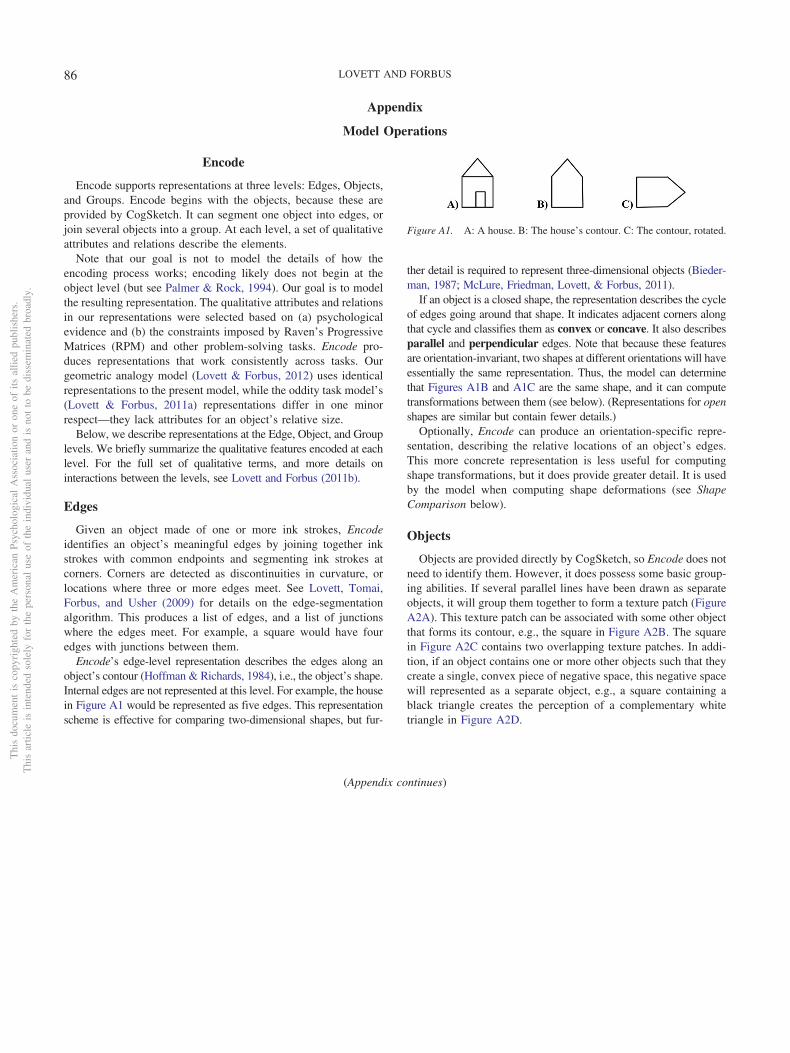
Appendix

Model Operations

Encode

Encode supports representations at three levels: Edges, Objects,and Groups. Encode begins with the objects, because these areprovided by CogSketch. It can segment one object into edges, orjoin several objects into a group. At each level, a set of qualitativeattributes and relations describe the elements.

Note that our goal is not to model the details of how theencoding process works; encoding likely does not begin at theobject level (but see Palmer & Rock, 1994). Our goal is to modelthe resulting representation. The qualitative attributes and relationsin our representations were selected based on (a) psychologicalevidence and (b) the constraints imposed by Raven’s ProgressiveMatrices (RPM) and other problem-solving tasks. Encode pro-duces representations that work consistently across tasks. Ourgeometric analogy model (Lovett & Forbus, 2012) uses identicalrepresentations to the present model, while the oddity task model’s(Lovett & Forbus, 2011a) representations differ in one minorrespect—they lack attributes for an object’s relative size.

Below, we describe representations at the Edge, Object, and Grouplevels. We briefly summarize the qualitative features encoded at eachlevel. For the full set of qualitative terms, and more details oninteractions between the levels, see Lovett and Forbus (2011b).

Edges

Given an object made of one or more ink strokes, Encodeidentifies an object’s meaningful edges by joining together inkstrokes with common endpoints and segmenting ink strokes atcorners. Corners are detected as discontinuities in curvature, orlocations where three or more edges meet. See Lovett, Tomai,Forbus, and Usher (2009) for details on the edge-segmentationalgorithm. This produces a list of edges, and a list of junctionswhere the edges meet. For example, a square would have fouredges with junctions between them.

Encode’s edge-level representation describes the edges along anobject’s contour (Hoffman & Richards, 1984), i.e., the object’s shape.Internal edges are not represented at this level. For example, the housein Figure A1 would be represented as five edges. This representationscheme is effective for comparing two-dimensional shapes, but fur-

ther detail is required to represent three-dimensional objects (Bieder-man, 1987; McLure, Friedman, Lovett, & Forbus, 2011).

If an object is a closed shape, the representation describes the cycleof edges going around that shape. It indicates adjacent corners alongthat cycle and classifies them as convex or concave. It also describesparallel and perpendicular edges. Note that because these featuresare orientation-invariant, two shapes at different orientations will haveessentially the same representation. Thus, the model can determinethat Figures A1B and A1C are the same shape, and it can computetransformations between them (see below). (Representations for openshapes are similar but contain fewer details.)

Optionally, Encode can produce an orientation-specific repre-sentation, describing the relative locations of an object’s edges.This more concrete representation is less useful for computingshape transformations, but it does provide greater detail. It is usedby the model when computing shape deformations (see ShapeComparison below).

Objects

Objects are provided directly by CogSketch, so Encode does notneed to identify them. However, it does possess some basic group-ing abilities. If several parallel lines have been drawn as separateobjects, it will group them together to form a texture patch (FigureA2A). This texture patch can be associated with some other objectthat forms its contour, e.g., the square in Figure A2B. The squarein Figure A2C contains two overlapping texture patches. In addi-tion, if an object contains one or more other objects such that theycreate a single, convex piece of negative space, this negative spacewill represented as a separate object, e.g., a square containing ablack triangle creates the perception of a complementary whitetriangle in Figure A2D.

(Appendix continues)

Figure A1. A: A house. B: The house’s contour. C: The contour, rotated.

Thi

sdo

cum

ent

isco

pyri

ghte

dby

the

Am

eric

anPs

ycho

logi

cal

Ass

ocia

tion

oron

eof

itsal

lied

publ

ishe

rs.

Thi

sar

ticle

isin

tend

edso

lely

for

the

pers

onal

use

ofth

ein

divi

dual

user

and

isno

tto

bedi

ssem

inat

edbr

oadl

y.


The object-level representation includes attributes for color,texture, closure, curvedness, symmetry, and size (based on theoverall distribution of sizes in the problem). There are relations forrelative position, topology, and shape transformations (i.e., rota-tions, reflections, and changes in scale between objects in animage—see the next section on Compare Shapes).

Groups

Encode groups objects together based on the Gestalt groupingrules of similarity, proximity, and good continuation (Wertheimer,1938). For several objects to be grouped together, they must be ofsimilar size and shape (based on their object-level attributes); theymust be equidistant from each other; and they must be aligned withthe grouping’s orientation. In Figures A3A and A3C, the circleswould be joined into a single group. In A3B there would be twogroups, based on proximity. In A3D the triangles would begrouped, but in A3E they would not because they don’t align withthe grouping’s orientation. In A3F, the image’s topology breaksthe circles into two groups.

The group-level representation describes any groups, as well asany individual objects that failed to group. For example, FigureA3F would contain two groups and one individual object: therectangle. In many cases a group-level representation will containno groups at all, and so it will be identical to the object level. Thequalitative relations at the group level are similar to those at theobject level.

Compare Shapes

Shape transformations are computed using the shape compari-son strategy described previously: (a) Compare edge-level repre-sentations with Structure-Mapping Engine (SME), get correspond-ing edges; (b) take one pair of corresponding edges and computea quantitative transformation between them, consisting of a rota-tion or reflection, a size change, and a translation; and (c) applythis transformation to the quantitative edges in the first object,checking whether the transformed edges match those in the second

object, in terms of their orientation, length, location, and curved-ness. Note that a rotation of approximately 0°, combined with ascaling factor of about 1.0, indicates that the objects are identical.

For shape transformations, there is a single quantitative trans-formation that transforms all edges in the first shape into theircorresponding edges in the second shape. For shape deformations,however, the model computes separate transformations for eachpair of corresponding edges, as follows: For lengthening (Figure13A), two edges about a central axis become longer. Other edgeschange (translating or becoming longer or shorter) to accommo-date the changes in the lengths of the two central edges. Forpart-lengthening (Figure 13B), two edges along the bounds of onepart become longer (parts are defined by concave corners, Hoff-man & Richards, 1984). Again, other edges change to accommo-date. For part-addition (Figure 13C), new edges are added to theshape to produce an additional part (again, defined by concavecorners), and other edges change to accommodate. Finally, forsubshape (Figure 8), there is a perfect identity match between thecorresponding edges in two shapes, but one shape has additionaledges.

Within the current model, the subshape deformation is neverencoded as a difference between two images (e.g., when repre-senting a row of differences with Find Differences). It is only usedto guide basic perceptual reorganization.

For group transformations, the two groups’ object-level repre-sentations are compared to identity corresponding objects. Then,one pair of corresponding objects are compared to check if they arethe same shape. Group transformations are only encoded forgroups whose objects are the same shape (e.g., two groups ofcircles).

For groups, rotations, reflections, and deformations are notconsidered. The only possibilities are (a) there is a perfect identitymatch between corresponding objects within the groups (indicatesidentical groups, a larger group, or object to group, depending onthe number of objects in each group) or (b) there is not an identitymatch between corresponding objects (indicates a different groupstransformation).

Figure A2. Examples of texture patches and negative space.

Figure A3. Grouping examples.


Thi

sdo

cum

ent

isco

pyri

ghte

dby

the

Am

eric

anPs

ycho

logi

cal

Ass

ocia

tion

oron

eof

itsal

lied

publ

ishe

rs.

Thi

sar

ticle

isin

tend

edso

lely

for

the

pers

onal

use

ofth

ein

divi

dual

user

and

isno

tto

bedi

ssem

inat

edbr

oadl

y.


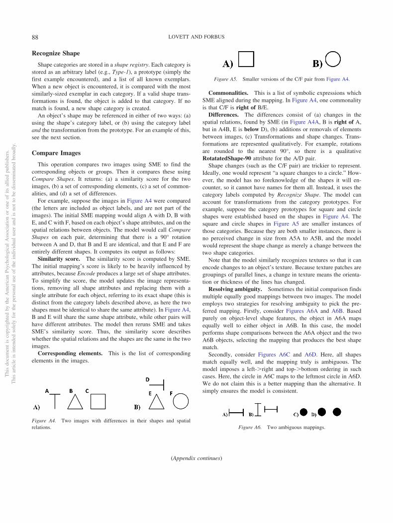
Recognize Shape

Shape categories are stored in a shape registry. Each category isstored as an arbitrary label (e.g., Type-1), a prototype (simply thefirst example encountered), and a list of all known exemplars.When a new object is encountered, it is compared with the mostsimilarly-sized exemplar in each category. If a valid shape trans-formations is found, the object is added to that category. If nomatch is found, a new shape category is created.

An object’s shape may be referenced in either of two ways: (a)using the shape’s category label, or (b) using the category labeland the transformation from the prototype. For an example of this,see the next section.

Compare Images

This operation compares two images using SME to find thecorresponding objects or groups. Then it compares these usingCompare Shapes. It returns: (a) a similarity score for the twoimages, (b) a set of corresponding elements, (c) a set of common-alities, and (d) a set of differences.

For example, suppose the images in Figure A4 were compared(the letters are included as object labels, and are not part of theimages). The initial SME mapping would align A with D, B withE, and C with F, based on each object’s shape attributes, and on thespatial relations between objects. The model would call CompareShapes on each pair, determining that there is a 90° rotationbetween A and D, that B and E are identical, and that E and F areentirely different shapes. It computes its output as follows:

Similarity score. The similarity score is computed by SME.The initial mapping’s score is likely to be heavily influenced byattributes, because Encode produces a large set of shape attributes.To simplify the score, the model updates the image representa-tions, removing all shape attributes and replacing them with asingle attribute for each object, referring to its exact shape (this isdistinct from the category labels described above, as here the twoshapes must be identical to share the same attribute). In Figure A4,B and E will share the same shape attribute, while other pairs willhave different attributes. The model then reruns SME and takesSME’s similarity score. Thus, the similarity score describeswhether the spatial relations and the shapes are the same in the twoimages.

Corresponding elements. This is the list of correspondingelements in the images.

Commonalities. This is a list of symbolic expressions whichSME aligned during the mapping. In Figure A4, one commonalityis that C/F is right of B/E.

Differences. The differences consist of (a) changes in thespatial relations, found by SME (in Figure A4A, B is right of A,but in A4B, E is below D), (b) additions or removals of elementsbetween images, (c) Transformations and shape changes. Trans-formations are represented qualitatively. For example, rotationsare rounded to the nearest 90°, so there is a qualitativeRotatatedShape-90 attribute for the A/D pair.

Shape changes (such as the C/F pair) are trickier to represent.Ideally, one would represent “a square changes to a circle.” How-ever, the model has no foreknowledge of the shapes it will en-counter, so it cannot have names for them all. Instead, it uses thecategory labels computed by Recognize Shape. The model canaccount for transformations from the category prototypes. Forexample, suppose the category prototypes for square and circleshapes were established based on the shapes in Figure A4. Thesquare and circle shapes in Figure A5 are smaller instances ofthose categories. Because they are both smaller instances, there isno perceived change in size from A5A to A5B, and the modelwould represent the shape change as merely a change between thetwo shape categories.

Note that the model similarly recognizes textures so that it canencode changes to an object’s texture. Because texture patches aregroupings of parallel lines, a change in texture means the orienta-tion or thickness of the lines has changed.

Resolving ambiguity. Sometimes the initial comparison findsmultiple equally good mappings between two images. The modelemploys two strategies for resolving ambiguity to pick the pre-ferred mapping. Firstly, consider Figures A6A and A6B. Basedpurely on object-level shape features, the object in A6A mapsequally well to either object in A6B. In this case, the modelperforms shape comparisons between the A6A object and the twoA6B objects, selecting the mapping that produces the best shapematch.

Secondly, consider Figures A6C and A6D. Here, all shapesmatch equally well, and the mapping truly is ambiguous. Themodel imposes a left-�right and top-�bottom ordering in suchcases. Here, the circle in A6C maps to the leftmost circle in A6D.We do not claim this is a better mapping than the alternative. Itsimply ensures the model is consistent.


Figure A4. Two images with differences in their shapes and spatialrelations.

Figure A5. Smaller versions of the C/F pair from Figure A4.

Figure A6. Two ambiguous mappings.

Thi

sdo

cum

ent

isco

pyri

ghte

dby

the

Am

eric

anPs

ycho

logi

cal

Ass

ocia

tion

oron

eof

itsal

lied

publ

ishe

rs.

Thi

sar

ticle

isin

tend

edso

lely

for

the

pers

onal

use

ofth

ein

divi

dual

user

and

isno

tto

bedi

ssem

inat

edbr

oadl

y.


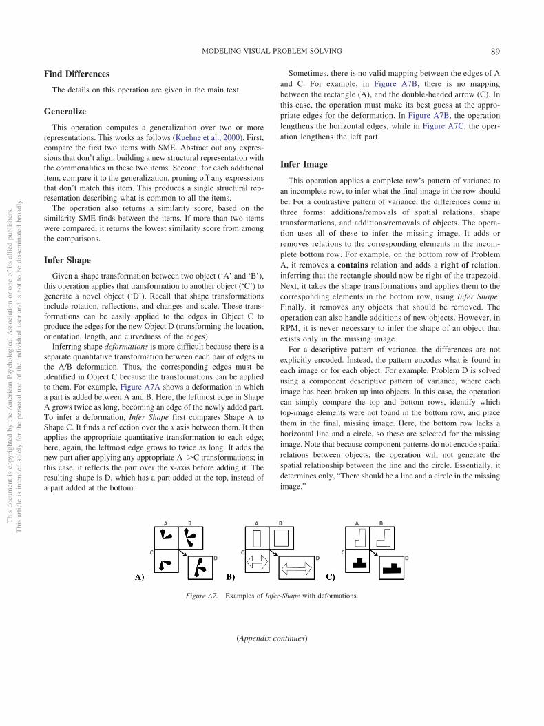
Find Differences

The details on this operation are given in the main text.

Generalize

This operation computes a generalization over two or morerepresentations. This works as follows (Kuehne et al., 2000). First,compare the first two items with SME. Abstract out any expres-sions that don’t align, building a new structural representation withthe commonalities in these two items. Second, for each additionalitem, compare it to the generalization, pruning off any expressionsthat don’t match this item. This produces a single structural rep-resentation describing what is common to all the items.

The operation also returns a similarity score, based on thesimilarity SME finds between the items. If more than two itemswere compared, it returns the lowest similarity score from amongthe comparisons.

Infer Shape

Given a shape transformation between two object (‘A’ and ‘B’),this operation applies that transformation to another object (‘C’) togenerate a novel object (‘D’). Recall that shape transformationsinclude rotation, reflections, and changes and scale. These trans-formations can be easily applied to the edges in Object C toproduce the edges for the new Object D (transforming the location,orientation, length, and curvedness of the edges).

Inferring shape deformations is more difficult because there is aseparate quantitative transformation between each pair of edges inthe A/B deformation. Thus, the corresponding edges must beidentified in Object C because the transformations can be appliedto them. For example, Figure A7A shows a deformation in whicha part is added between A and B. Here, the leftmost edge in ShapeA grows twice as long, becoming an edge of the newly added part.To infer a deformation, Infer Shape first compares Shape A toShape C. It finds a reflection over the x axis between them. It thenapplies the appropriate quantitative transformation to each edge;here, again, the leftmost edge grows to twice as long. It adds thenew part after applying any appropriate A–�C transformations; inthis case, it reflects the part over the x-axis before adding it. Theresulting shape is D, which has a part added at the top, instead ofa part added at the bottom.

Sometimes, there is no valid mapping between the edges of Aand C. For example, in Figure A7B, there is no mappingbetween the rectangle (A), and the double-headed arrow (C). Inthis case, the operation must make its best guess at the appro-priate edges for the deformation. In Figure A7B, the operationlengthens the horizontal edges, while in Figure A7C, the oper-ation lengthens the left part.

Infer Image

This operation applies a complete row’s pattern of variance toan incomplete row, to infer what the final image in the row shouldbe. For a contrastive pattern of variance, the differences come inthree forms: additions/removals of spatial relations, shapetransformations, and additions/removals of objects. The opera-tion uses all of these to infer the missing image. It adds orremoves relations to the corresponding elements in the incom-plete bottom row. For example, on the bottom row of ProblemA, it removes a contains relation and adds a right of relation,inferring that the rectangle should now be right of the trapezoid.Next, it takes the shape transformations and applies them to thecorresponding elements in the bottom row, using Infer Shape.Finally, it removes any objects that should be removed. Theoperation can also handle additions of new objects. However, inRPM, it is never necessary to infer the shape of an object thatexists only in the missing image.

For a descriptive pattern of variance, the differences are notexplicitly encoded. Instead, the pattern encodes what is found ineach image or for each object. For example, Problem D is solvedusing a component descriptive pattern of variance, where eachimage has been broken up into objects. In this case, the operationcan simply compare the top and bottom rows, identify whichtop-image elements were not found in the bottom row, and placethem in the final, missing image. Here, the bottom row lacks ahorizontal line and a circle, so these are selected for the missingimage. Note that because component patterns do not encode spatialrelations between objects, the operation will not generate thespatial relationship between the line and the circle. Essentially, itdetermines only, “There should be a line and a circle in the missingimage.”

Figure A7. Examples of Infer-Shape with deformations.


Thi

sdo

cum

ent

isco

pyri

ghte

dby

the

Am

eric

anPs

ycho

logi

cal

Ass

ocia

tion

oron

eof

itsal

lied

publ

ishe

rs.

Thi

sar

ticle

isin

tend

edso

lely

for

the

pers

onal

use

ofth

ein

divi

dual

user

and

isno

tto

bedi

ssem

inat

edbr

oadl

y.


Detect Texture

This operation detects textures using a simplified representation.Given an image, it prints all the objects in the image to a bit-map—a 2 � 2 array of points which makes no distinction betweenone object and another. It then scans along a corridor of the bitmap(Figure 11) to see if there is a repeating texture.

Detect Texture uses autocorrelation (Oppenheim & Schafer,2009), a common approach from signal processing, to detectrepeating patterns in a corridor. The idea is to divide the signal intowindows and check whether consecutive windows correlate witheach other. One varies the window length to find the best corre-lation. Here, each window is a portion of the corridor’s totallength.

Detect Texture computes two signals from a window: rows andcolumns. For rows, it takes each row of the window and adds upthe pixels that are “on,” i.e., those that are not empty space.

Similarly, it takes each column of the window and adds up thepixels that are “on.” In computing the correlation between twowindows, Detect Texture takes the lower of the correlation be-tween rows and the correlation between columns.

A row’s overall score is the minimum correlation value for alladjacent windows. If this score exceeds a threshold (0.85), theoperation is a success. It returns the score and the window size thatproduced this score.

Autocorrelation is a useful tool for detecting repeating patternsin an image. However, we view this as only an approximation ofhuman texture detection—accurately modeling low-level texturedetection is not a priority for this work. For a more in-depth modelof texture processing, see (Stevens, 1981).

Received April 14, 2015Revision received July 1, 2016

Accepted July 1, 2016 �

Thi

sdo

cum

ent

isco

pyri

ghte

dby

the

Am

eric

anPs

ycho

logi

cal

Ass

ocia

tion

oron

eof

itsal

lied

publ

ishe

rs.

Thi

sar

ticle

isin

tend

edso

lely

for

the

pers

onal

use

ofth

ein

divi

dual

user

and

isno

tto

bedi

ssem

inat

edbr

oadl

y.


Modeling Visual Problem Solving as Analogical Reasoning · Andrew Lovett and Kenneth Forbus...

Documents

Transcript of Modeling Visual Problem Solving as Analogical Reasoning · Andrew Lovett and Kenneth Forbus...