MODELING THE TRANSPORT OF SAND AND MUD IN THE MINNESOTA RIVER

BY

CHUAN LI

THESIS

Submitted in partial fulfillment of the requirements

for the degree of Master of Science in Civil Engineering

in the Graduate College of the

University of Illinois at Urbana-Champaign, 2014

Urbana, Illinois

Advisers:

Professor Gary Parker

Assistant Professor Enrica Viparelli, University of South Carolina

ii

ABSTRACT

This thesis is organized into two chapters. The first chapter presents a study on the

bankfull characteristics of rivers. The bankfull geometry of alluvial rivers is thought to be

controlled by water and sediment supply, and characteristic sediment size. Here we demonstrate

a novel finding: when bankfull shear velocity and bankfull depth are correlated against bed

material grain size and bed slope, they are to first order independent of grain size and dependent

on water viscosity. We demonstrate this using a similarity collapse for bankfull Shields number

as a function of slope and grain size, obtained with data for 230 river reaches ranging from silt-

bed to cobble-bed. Our analysis shows that bankfull Shields number increases with slope to

about the half power. We show that the new relation for bankfull Shields number provides more

realistic predictions for the downstream variation of bankfull characteristics of rivers than a

previously used assumption of constant bankfull Shields number.

The second chapter presents a study on sediment routing of the Minnesota River. We

perform, via numerical modeling, an analysis of the response of the Minnesota River to changes

in sediment loading. To achieve this, we developed a one-dimensional, coupled flow, sediment

transport, and channel bed/floodplain morphodynamics model and derived model inputs from

field parameters where possible. We show that sediment output from the system is

predominantly wash load, and that changes in bed material input has little effect on sediment

output in 600 years. However, changes in wash load input has a near-immediate effect on

sediment output. Thus, reducing input of wash load would have greater impact on sediment yield

of the Minnesota River than reducing input of bed material load.

iii

ACKNOWLEDGEMENTS

This thesis would not have been possible without the support of many people. First I

would like to thank my advisers, Professors Gary Parker and Enrica Viparelli, for their guidance

and understanding. I thank the faculty of the University of Illinois, the College of Engineering,

and the Department of Civil and Environmental Engineering for the excellent education. In

particular I thank Professors Barbara Minsker and Albert Valocchi for their mentorship and

advice. I thank the National Science Foundation, in particular the Graduate Research Fellowship

Program, for the financial support.

I would also like to thank all the students I have had the pleasure to study and work with,

in particular those in the Ven Te Chow Hydrosystems Laboratory. I thank especially my lab-

mates: Matt Czapiga, Andrew Rehn, Roberto Fernández, Jeffrey Kwang, Esther Eke, Ruiyu

Wang, Rossella Luchi, and Anna Pelosi for their support and companionship. Many thanks to all

my friends and family. Last but not least, I thank my parents for their love and support.

iv

TABLE OF CONTENTS

CHAPTER 1 VARIABLE SHIELDS NUMBER MODEL FOR RIVER BANKFULL

GEOMETRY: BANKFULL SHEAR VELOCITY IS VISCOSITY-DEPENDENT BUT GRAIN

SIZE- INDEPENDENT ..............................................................................................................1

1.1 INTRODUCTION .............................................................................................................1

1.2 FORMULATION OF THE NEW RELATION FOR BANKFULL SHIELDS NUMBER ..2

1.3 IMPLICATIONS FOR BANKFULL SHEAR VELOCITY AND DEPTH .........................4

1.4 GENERAL RELATIONS FOR BANKFULL CHARACTERISTICS ................................7

1.5 RELATIONS FOR BANKFULL CHARACTERISTICS FOR SAND-BED STREAMS ...8

1.6 COMPARISON OF BANKFULL CHARACTERISTICS RELATIONS FOR SAND-BED

STREAMS: FROM CONSTANT SHIELDS NUMBER VERSUS THE PROPOSED

FORMULATION .................................................................................................................. 10

1.7 APPLICATION TO MORPHODYNAMIC MODELING: CASE OF THE FLY-

STRICKLAND RIVER SYSTEM, PAPUA NEW GUINEA ................................................. 11

1.8 DISCUSSION: APPLICATION TO MODERN SEA LEVEL RISE DRIVEN BY

CLIMATE CHANGE ............................................................................................................ 15

1.9 CONCLUSIONS ............................................................................................................. 16

CHAPTER 2 RESPONSE OF THE MINNESOTA RIVER TO VARIANT SEDIMENT

LOADING ................................................................................................................................ 30

2.1 INTRODUCTION ........................................................................................................... 30

2.2 STUDY AREA ................................................................................................................ 30

2.3 METHOD ........................................................................................................................ 31

2.4 RESULTS AND DISCUSSION ....................................................................................... 36

REFERENCES ......................................................................................................................... 64

This chapter contains materials accepted for publication by the Journal of Hydraulic Research.

The co-authors are: Chuan Li, Matthew J. Czapiga, Esther E. Eke, Enrica Viparelli, Gary Parker 1

CHAPTER 1

VARIABLE SHIELDS NUMBER MODEL FOR RIVER BANKFULL GEOMETRY:

BANKFULL SHEAR VELOCITY IS VISCOSITY-DEPENDENT BUT GRAIN SIZE-

INDEPENDENT

1.1 INTRODUCTION

The bankfull geometry of alluvial rivers is characterized in terms of bankfull width Bbf,

bankfull depth Hbf and bankfull discharge Qbf (Leopold and Maddock 1953). The physics

behind these relations also involves characteristic bed material grain size D, submerged specific

gravity of sediment R (~ 1.65 for quartz), water viscosity ν, bed slope S and total volume bed

material load (bedload plus suspended bed material load) Qtbf at bankfull flow (Parker et al.

2007, Wilkerson and Parker 2011).

A central question of river hydraulics is how channel characteristics vary with flood

discharge, sediment supply and sediment size. The problem can be characterized in terms of

relations for Bbf, Hbf and S as functions of Qbf, Qtbf and D. Earlier attempts to specify closures for

these relations have assumed a specified formative (bankfull) channel Shields number τ*bf (Paola

et. al 1992, Parker et al. 1998a, 1998b). The bankfull Shields number is useful as part of a

closure scheme for bankfull geometry because it provides, under the approximation of steady,

uniform flow, a relation for the product of bankfull depth and bed slope. Based on earlier work

of Parker (1978), Paola et al. (1992) first used the assumption of constant bankfull Shields

number to study the response of a gravel-bed river profile to subsidence. The corresponding

assumption for sand-bed rivers, but with a much higher bankfull Shields number, has been

implemented by Parker et al. (1998a, 1998b). With a relatively sparse data set, Parker et al.

(1998a, 1998b) found that the bankfull Shields number in alluvial streams could be crudely

approximated invariant to other characteristics of rivers, e.g. bed slope. The constant values

0.042 (Parker et al. 1998a) or 0.049 (Parker 2004) have been suggested for gravel-bed rivers, and

the constant values 1.8 (Parker et al. 1998b) or 1.86 (Parker 2004, Parker et al. 2008) have been

used for sand-bed rivers. These authors used the assumption of a constant formative Shields

2

number, combined with momentum balance, continuity relations for water and bed material load,

and bed material sediment transport equations, to develop predictive relations for bankfull

width, bankfull depth and bed slope as functions of bankfull discharge and bed material transport

at bankfull flow. The resulting relations have been applied to study how rivers respond to basin

subsidence and rising base level (Paola et. al 1992, Parker 2004, Parker et al. 1998b) and how

deltas evolve (Kim et al. 2009).

Here we rely on three compendiums of data on bankfull characteristics of single-thread

alluvial channels to revisit the empirical formulation for bankfull Shields number (Parker et al.

2007, Wilkerson and Parker 2011, Latrubesse, personal communication). The data base includes

230 river reaches, with Qbf varying from 0.34 to 216,340 m3/s, Bbf varying from 2.3 to 3,400 m,

Hbf varying from 0.22 to 48.1 m, S varying from 8.8 10-6 to 5.2 10-2, and D varying from

0.04 to 168 mm. One reach from the original data was omitted as the representative grain size

was much finer than the other reaches.

The data used in Parker et al. (2007) pertain to rivers for which D 25 mm. They were

obtained from 4 sources, the references for which are documented in the original paper on page 3

and the list of references. The data used in Wilkerson et al. (2011) pertain to rivers for which D <

25 mm. They were obtained from 26 sources, the references for which are documented in the

original paper in Table 1 and the list of references. The data from Latrubesse (personal

communication) pertain to tropical sand-bed rivers, most of them very large (i.e. bankfull

discharge ≥ 20,000 m3/s). These data were screened in detail to determine suitability for analysis.

For example, the large data set of Soar and Thorne (2001) was excluded because bankfull

discharge was computed rather than measured. The entire data set used in this study can be

downloaded from the site:

http://hydrolab.illinois.edu/people/parkerg//VariableShieldsModelBasicData.htm.

1.2 FORMULATION OF THE NEW RELATION FOR BANKFULL SHIELDS NUMBER

The text given here is based on a paper, Li et al. (accepted), that has been accepted for

publication in the Journal of Hydraulic Research as of May, 2014.

We estimate bankfull boundary shear stress τbf using the normal flow approximation for

momentum balance:

3

bf bfgH S ,

(1.1)

where ρ is water density and g is gravitational acceleration. The dimensionless Shields number is

bf

bfRgD

. (1.2)

Here R = 1.65 is the submerged specific gravity for quartz. Between Eqs. (1.1) and (1.2),

bf

bf

H S

RD

.

(1.3)

We define dimensionless grain size D* as (van Rijn 1984)

1/3

2/3

RgD D

,

(1.4)

where denotes the kinematic viscosity of water. In all the calculations here, is assumed to

take the value 1 × 10-6 m2/s in the absence of direct measurements. It is worth noting, however,

that for water, varies only from 1.52 × 10-6 m2/s to 0.80×10-6 m2/s as temperature varies from

5C to 30C.

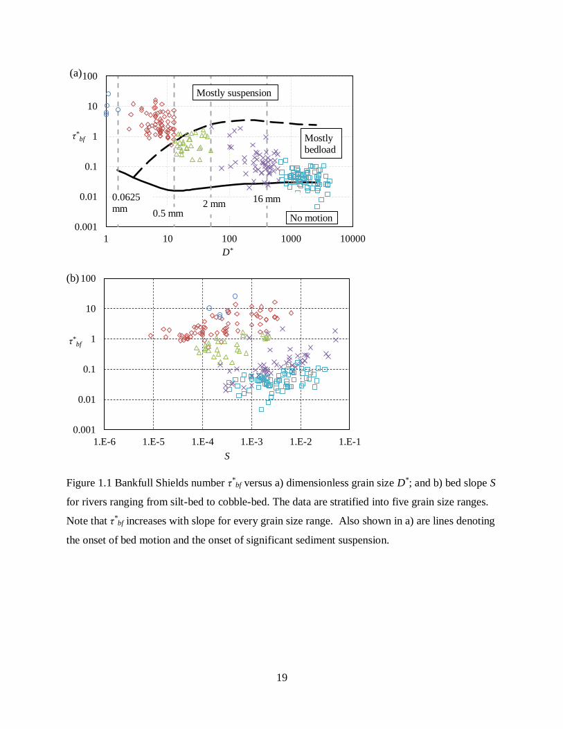
Figure 1.1a shows a plot of τ*bf versus D* in the form of a Shields diagram (Parker et al.

2008), with lines indicating the approximate inception of bedload transport and the approximate

initiation of significant suspension. The data have been stratified into five grain size ranges: 0.04

– 0.062 mm (silt), 0.062 – 0.5 mm (very fine to medium sand), 0.5 – 2 mm (coarse to very coarse

sand), 2 – 25 mm (fine to coarse gravel) and 25 – 168 mm (coarse gravel to cobbles). The data

cover the range from suspended load-dominated rivers to bedload-dominated rivers. The figure

shows a consistent trend, with τ*bf decreasing with increasing D*, that has been noted earlier by

Dade and Friend (1998).

Figure 1.1b shows a corresponding plot of τ*bf versus bed slope S, with the same grain

size discrimination: it is seen that τ*bf is an increasing function of S through every grain size

range. While a tendency for critical Shields number (corresponding to the onset of motion) to

increase with S has been reported previously (Lamb et al. 2008, Recking 2009), here we

demonstrate this tendency for bankfull Shields number as well. This tendency was first noted for

a data set corresponding to D ranging from 17 mm to 36 mm (Mueller and Pitlick, 2005) here we

demonstrate it over D ranging from 0.04 mm to 168 mm.

4

Figure 1.1 suggests the use of similarity collapse to obtain a universal relation for τ*bf as a

function of S and D*. We performed the analysis by seeking an exponent m in the relation τ*bf ~

Sm, applicable to all grain sizes, and then performing a power regression analysis of τ*bf/S

m versus

D*. The relation so obtained is τ*bf = 1223(D*)-1.00S0.534, with a coefficient of determination R2 =

0.948, as shown in Figure 1.2. Rounding appropriately,

1

m

bf D S

,

(1.5)

where β = 1220 and m = 0.53.

The conclusion in Eq. (1.5) that the exponent of D* is - 1.00 is confirmed by splitting the data

into two subsets, one for which D 25 mm and one for which D > 25 mm. The corresponding

exponents of D* are – 1.096 and – 1.048, i.e. only a very modest deviation from – 1.00. It is seen

from Eq. (1.4) that D* depends on-2/3. As noted above, has been set equal to 1×10-6 m2/s, i.e.

the standard value for water. In order to study the effect of varying , this parameter was

randomized between the values 0.80×10-6 m2/s (30C) and 1.52×10-6 m2/s (5C). The

randomization was different for each river reach. Ten implementations of this randomization

yielded exponents ranging from – 0.9904 to – 1.0004.

1.3 IMPLICATIONS FOR BANKFULL SHEAR VELOCITY AND DEPTH

The value of the exponent of D* in Eq. (1.5), i.e. -1, has an unexpected consequence. The

definition for τ*bf of Eq. (1.2) is such that it varies as D-1, but the right-hand side of Eq. (1.5) also

varies as D-1. Defining bankfull shear velocity u*bf as

1/2

bf

bfu

,

(1.6)

it follows that bed material grain size precisely cancels out in the relation for bankfull shear

velocity from Eqs. (1.2), (1.5), and (1.6). With the aid of Eq. (1.5), Eq. (1.3) can be solved for

Hbf; and the bed material grain size again cancels out in the relation for bankfull water depth.

The present analysis thus yields a remarkable, and indeed counterintuitive result: bankfull

shear velocity and bankfull depth do not depend on the characteristic grain size of the bed

material, as shown by the resulting dimensionless relations,

5

0.26 0.4735.0 , 1220bf bfu S H S

, (1.7a, b)

where the dimensionless shear velocity u*bf and depth Hbf are

1/3

1/3 2/3,

( )

bf bf

bf bf

u H gu H

RRg

.

(1.8a, b)

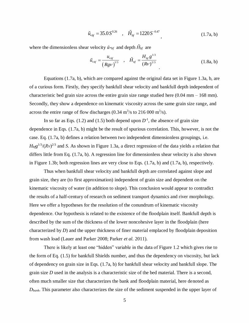
Equations (1.7a, b), which are compared against the original data set in Figure 1.3a, b, are

of a curious form. Firstly, they specify bankfull shear velocity and bankfull depth independent of

characteristic bed grain size across the entire grain size range studied here (0.04 mm – 168 mm).

Secondly, they show a dependence on kinematic viscosity across the same grain size range, and

across the entire range of flow discharges (0.34 m3/s to 216 000 m3/s).

In so far as Eqs. (1.2) and (1.5) both depend upon D-1, the absence of grain size

dependence in Eqs. (1.7a, b) might be the result of spurious correlation. This, however, is not the

case. Eq. (1.7a, b) defines a relation between two independent dimensionless groupings, i.e.

Hbfg1/3/(Rν)2/3 and S. As shown in Figure 1.3a, a direct regression of the data yields a relation that

differs little from Eq. (1.7a, b). A regression line for dimensionless shear velocity is also shown

in Figure 1.3b; both regression lines are very close to Eqs. (1.7a, b) and (1.7a, b), respectively.

Thus when bankfull shear velocity and bankfull depth are correlated against slope and

grain size, they are (to first approximation) independent of grain size and dependent on the

kinematic viscosity of water (in addition to slope). This conclusion would appear to contradict

the results of a half-century of research on sediment transport dynamics and river morphology.

Here we offer a hypotheses for the resolution of the conundrum of kinematic viscosity

dependence. Our hypothesis is related to the existence of the floodplain itself. Bankfull depth is

described by the sum of the thickness of the lower noncohesive layer in the floodplain (here

characterized by D) and the upper thickness of finer material emplaced by floodplain deposition

from wash load (Lauer and Parker 2008; Parker et al. 2011).

There is likely at least one “hidden” variable in the data of Figure 1.2 which gives rise to

the form of Eq. (1.5) for bankfull Shields number, and thus the dependency on viscosity, but lack

of dependency on grain size in Eqs. (1.7a, b) for bankfull shear velocity and bankfull slope. The

grain size D used in the analysis is a characteristic size of the bed material. There is a second,

often much smaller size that characterizes the bank and floodplain material, here denoted as

Dbank. This parameter also characterizes the size of the sediment suspended in the upper layer of

6

the water column that spills onto, and emplaces the floodplain when the river goes overbank. As

seen from Figure 1.1, this size is likely to be less than 0.5 mm. It is thus in a grain size range

where fall velocity is a strong function of Reynolds number. More specifically, dimensionless

fall velocity Rf,bank = vs,bank / (RgDbank)1/2, where vs,bank is the fall velocity associated with a

characteristic diameter of the size Dbank, is related to D*bank = (Rg)1/3Dbank / ν

2/3 through standard

relations for fall velocity (e.g. Dietrich 1982). For example, Eq. (1.7a, b) can be rewritten as

1/20.2635.0

bf

bank

bank

uD S

RgD

, (1.9)

thus illustrating how viscosity can enter the problem across scales.

An independent data set on gravel-bed rivers is available to evaluate the hypothesis of

viscosity dependence via fine-grained material from which the floodplain is constructed. The

data set of Hey and Thorne (1986) includes 62 river reaches, divided into four classes,

Vegetation Types I, II, III and IV in accordance to increasing bank height and floodplain

vegetation density. In addition to the parameters specified above, that data also include bank

material size Dbank for 58 of the reaches. Hey and Thorne (1986) indicate that higher vegetation

density correlates with narrower and deeper reaches. It is a reasonable inference that narrower

and deeper reaches have thicker floodplains characterized by the size Dbank rather than bed

material size D.

We first demonstrate that the data of Hey and Thorne (1986) show the same pattern as the

data used above. Figure 1.4a is a version of Figure 1.2, but in which the new data set has been

included. For each Vegetation Type the data are further partitioned between channels with bed

material greater than 25 mm (D > 25 mm in Figure 1.4 and Figure 1.5) and channels with bed

material finer than 25 mm (D < 25 mm in Figs. 4 and 5). The new data clearly follow the same

trend as the previously used data, to which Eq. (1.5) provides a good fit. Figure 1.4b shows an

expanded view of Figure 1.4a in which only the new data are plotted. Figure 1.4b shows a

tendency for τ*bf /S

0.53 to increase with increasing vegetation density. This can be inferred to be

associated with thicker floodplains emplaced by fine-grained material versus D* for their data,

along with Eq. (1.5). It is seen that the data generally follow Eq. (1.5), but also show a tendency

related to floodplain thickness. That is, the value of τ*bf /S

0.53 increases with increasing vegetation

density.

7

Figure 1.5a, b are versions of Figure 1.3a, b in which the new data have been added.

Again, the data fit well within previous data, and Eqs. (1.7a, b) provide reasonable fits. Thus the

new data tend to confirm the result that bankfull shear velocity and bankfull depth are, to first

order, dependent on viscosity but independent of bed material grain size.

Figure 1.6 shows a plot of dimensionless fall velocity Rf = vs/(RgD)1/2 versus D* =

(Rg)1/3D/2/3, where here vs is an arbitrary fall velocity and D is an arbitrary grain size. The curve

shown therein is that of Dietrich (1982). Also shown on the plot are the values of Rf,bank

computed from the same relation, using the grain size Dbank from the 58 reaches of the Hey and

Thorne (1986) for which Dbank is specified. It is important to keep in mind that Figure 1.6 is not a

comparison of measured versus predicted values. Instead, it shows that over the entire range of

the data of Hey and Thorne (1986), the fall velocity of the bank/floodplain material can be

expected to be strongly dependent on viscosity. It follows that bankfull Shields number and

bankfull depth can be expected to include a viscosity dependence, as long as fine-grained

material plays a substantial role in building the floodplain that confines the channel.

1.4 GENERAL RELATIONS FOR BANKFULL CHARACTERISTICS

The characteristic grain size of the bed material D, however, does indeed enter the picture

through predictive relations for Hbf, Bbf, and S as functions of Qbf and Qtbf. Such relations can be

derived by augmenting Eq. (1.5) with a) momentum balance as approximated by Eq. (1.1); b) the

continuity relations

,bf bf bf bf tbf tbf bfQ U H B Q q B , (1.10a, b)

where Ubf is bankfull flow velocity and qtbf is volume bed material transport rate per unit width

at bankfull flow; c) the definition of the dimensionless Chezy resistance coefficient Cz:

/

bf bf

bfbf

U UCz

u

,

(1.11)

d) a specification of Cz; and e) a predictor for qtbf.

The calculations can be performed for any pair of relations for Cz and qtbf. An example

generic relation for qtbf is

8

tn

tbf t s bf cq RgDD , (1.12)

where αt, φs, nt are arbitrary coefficients and exponent of the sediment transport relation (Parker,

2004). Equations (1.1), (1.2), (1.10a, b), (1.11), and (1.12) can be reduced to produce the three

relations for bankfull characteristics,

* *

1t

bf tbfn

t s bf c

B QRgDD

,

(1.13)

* *

*

tn

t s bf c bf

bf

tbfbf

D QH

QCz

,

(1.14)

3/2*

* * t

bf tbf

n

bft s bf c

R Cz QS

QR

.

(1.15)

Equations (1.13), (1.14), and (1.15) cannot be solved explicitly in terms of simple power

laws when τ*c is not equal to zero, because τ*

bf is a function of S as specified by Eq. (1.5). In this

case, an iterative technique may be useful to obtain a solution. The above relations are general,

and apply for any specification for τ*bf and Cz. The constant Shields formulation is recovered by

setting τ*bf and Cz to prescribed constants.

1.5 RELATIONS FOR BANKFULL CHARACTERISTICS FOR SAND-BED STREAMS

In the case of sand-bed streams, the Engelund-Hansen total bed material load relation

(Engelund and Hansen 1967),

5/2

2 , 0.05tbf EH bf EHq Cz RgD D ,

(1.16a, b)

is used because it is accurate for sand transport (Brownlie 1981) and allows solution in closed

form in terms of simple power laws that clearly elucidate the results.

The resistance coefficient Cz is often specified with a set value of Manning’s n, but this is

not reliable for e.g. rivers dominated by bedform resistance (Ferguson 2010). The subset of the

data used here corresponding to grain sizes between 0.0625 mm to 2 mm is thus used to find an

9

empirical relation between Cz at bankfull flow and bed slope S. Figure 1.7 shows Cz versus S for

the entire data set, as well as the regression relation

Rn

RCz S

, (1.17)

where αR = 2.53 and nR = 0.19, determined for the indicated subset. The data show substantial

scatter, which is to be expected in light of e.g. varying bedform regimes, bar configuration and

channel sinuosity. Equation (1.17), however, captures the overall trend for Cz to decline with

increasing S.

Equation (1.17) is an empirical relation that was first proposed in Chapter 3 of Parker

(2004). As noted above, it is likely superior to a formulation using Manning’s n, which needs to

be guessed or determined from site-specific data for most rivers (Ferguson 2010).

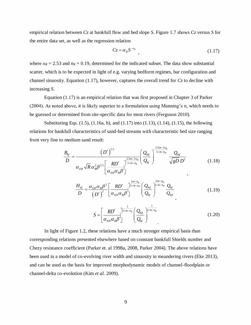
Substituting Eqs. (1.5), (1.16a, b), and (1.17) into (1.13), (1.14), (1.15), the following

relations for bankfull characteristics of sand-bed streams with characteristic bed size ranging

from very fine to medium sand result:

2.5 22.5

1

2.5 2 2

12 2.5

R

R

R

R

m n

m nbf tbf tbf

m n

bfm n

EH R

EH R

DB Q Q

D Q gD DRD

R

,

(1.18)

22

2 11

2

RR

RR

m nm n

m nm nbf tbf bfEH R

EH R bf tbf

H Q QRD

D Q QD

,

(1.19)

11

11 RRm nm n

tbf

EH R bf

QRDS

Q

.

(1.20)

In light of Figure 1.2, these relations have a much stronger empirical basis than

corresponding relations presented elsewhere based on constant bankfull Shields number and

Chezy resistance coefficient (Parker et. al 1998a, 2008, Parker 2004). The above relations have

been used in a model of co-evolving river width and sinuosity in meandering rivers (Eke 2013),

and can be used as the basis for improved morphodynamic models of channel-floodplain or

channel-delta co-evolution (Kim et al. 2009).

10

1.6 COMPARISON OF BANKFULL CHARACTERISTICS RELATIONS FOR SAND-BED

STREAMS: FROM CONSTANT SHIELDS NUMBER VERSUS THE PROPOSED

FORMULATION

In the case of constant τ*bf and Cz, Equations (1.13), (1.14), and (1.15) can be used to

express the exponent dependency of Hbf, Bbf, and S on Qbf, Qtbf, and D:

0 1 1.5

1 1 1

1 1 0

~

~

~

bf bf tbf

bf bf tbf

bf tbf

B Q Q D

H Q Q D

S Q Q D

.

(1.21a, b, c)

Similarly, exponents in Eqs. (1.18), (1.19), and (1.20) for the proposed formulation, with m =

0.53 and nR = 0.19, as determined for Eqs. (1.5) and (1.17), are, respectively:

0.71 0.29 0.29

0.35 0.35 0.35

0.75 0.75 0.75

~

~

~

bf bf tbf

bf bf tbf

bf tbf

B Q Q D

H Q Q D

S Q Q D

.

(1.22a, b, c)

The resulting equations with: constant bankfull Shields number, i.e. Eqs. (1.21a, b, c), and the

proposed relations, i.e. Eqs. (1.22a, b, c) give fundamentally different predictions for Bbf, Hbf, and

S.

In the proposed formulation, a) bankfull width increases with increasing flood discharge,

sand supply and sand size (with the respective exponents 0.71. 0.29 and 0.29); b) bankfull depth

increases with increasing flood discharge, and decreasing sand supply and sand size (with the

respective exponents 0.35, -0.35 and -0.35); and c) slope increases with decreasing flood

discharge, and increasing sand supply and sand size (with respective exponents -0.75, 0.75 and

0.75).

It is useful to recall that the correlation of bankfull Shields number with slope and grain

size specified by Eq. (1.5) dictates that bankfull shear velocity and bankfull depth are

independent of grain size (Eqs. (1.7a, b) and (1.8a, b)). Eqs. (1.22a, b, c), however, indicate that

when slope, bankfull width and bankfull depth are expressed as functions of the three parameters

bankfull discharge, sediment transport rate at bankfull discharge and grain size, all the relations

show a dependence on grain size. This is because grain size enters the formulation via Eq. (1.5)

11

for bankfull Shields number and Eq. (1.16a, b) for bed material transport rate, in both cases as

the inverse of grain size.

The constant bankfull Shields formulation of Eq. (1.21a, b, c) suggests that Bbf is

independent of Qbf, (with an exponent of 0) and strongly decreases with an increase in the

median grain size diameter (with an exponent of -1); this is quite divergent from our proposed

Eq. (1.22a, b, c) which shows strongest dependence on flood discharge (exponent of 0.71). In

addition, the dependency Hbf on Qbf and Qtbf on Hbf with our proposed Eq. (1.22a, b, c) is such

that the magnitude of the exponents are reduced by a factor of nearly three as compared to Eq.

(1.21a, b, c) for constant Shields number. The dependence of S on Qbf and Qtbf in our proposed

relation (1.22a, b, c) is similar to the constant Shields number Eq. (1.21a, b, c), but the

magnitude of the exponents are muted. Our proposed Eq. (1.22a, b, c) shows a strong

dependence of S on grain size (exponent of 0.75) whereas the constant Shields number Eq.

(1.21a, b, c) is independent of grain size.

1.7 APPLICATION TO MORPHODYNAMIC MODELING: CASE OF THE FLY-

STRICKLAND RIVER SYSTEM, PAPUA NEW GUINEA

The proposed relations for bankfull characteristics (i.e. Eqs. (1.18), (1.19), (1.20)) can be

used to model morphologic changes of a self-formed channel and adjacent floodplain. In order to

do this, it must be assumed that the change of a self-formed channel is slow enough that

floodplain morphology can keep up with it, so that the channel neither avulses during

aggradation or strongly incises during degradation.

Our relations for τ*bf and Cz, i.e. Eqs. (1.5) and (1.17), represent regression of data with

the scatter shown in Figure 1.2 and Figure 1.7. Thus in any application to a specific river, it is

appropriate to normalize Eqs. (1.5) and (1.17) relative to a known reference slope SR, at which

τ*bf takes the known reference value τ*

R and Cz takes the known reference value CzR. With this

in mind, Eqs. (1.5) and (1.17) are normalized to the respective forms

* *

m

bf R

R

S

S

,

(1.23)

12

Rn

R

R

SCz Cz

S

,

(1.24)

where the exponents m and nR are those of Eqs. (1.5) and (1.17), respectively. These exponents

maintain the trends captured in empirical relations, but emanate from a single data point rather

than regressed average of all data points. We re-evaluate Eqs. (1.18), (1.19), (1.20) with Eqs.

(1.23), (1.24) to the forms

2.5 2

1

2.5 2 2

12 * 2.5

*

1R

R

R

R

m n

m nbf tbf tbf

m n

bfm n

EH R R

EH R R R

B Q Q

D Q gD DR

R CzS Cz

,

(1.25)

22

11* 2

*

RR

RR

m nm n

m nm nbf tbf bf

EH R R

EH R R R bf tbf

H Q QRCz

D S Cz Q Q

,

(1.26)

11

11

*

R RRm n m nm n

tbfR

EH R R bf

QRSS

Cz Q

.

(1.27)

Parker et al. (2008b) and Lauer et al. (2008) have studied the response of the Fly-

Strickland River system to Holocene sea level rise due to deglaciation of 10 mm/year for 12,000

years. Large, low-slope rivers worldwide show the imprint of this rise. Parker et al. (2008b)

analyzed the problem in the context of the constant Shields number model for hydraulic

geometry. Here we show the differences in the results that arise when we instead apply our

proposed model.

The Fly-Strickland River system in Papua New Guinea drains an area of approximately

75 000 km2 and consists of the Strickland River, the Fly River and tributaries such as the Ok

Tedi (Figure 1.8). The Fly River is segmented into the Upper Fly, Middle Fly, and Lower Fly,

bounded by junctions with the Ok Tedi and Strickland Rivers, respectively. The confluence of

the Fly and the Strickland rivers is called Everill Junction (Parker et al. 2008).

The Fly-Strickland River system begins in the highlands, where the streams are

dominated by bedrock and gravel-bed morphologies. Farther downstream, as the slope gradient

decreases, both the Fly and Strickland rivers transition into fully alluvial gravel bed-streams

(Parker et al. 2008). Even farther downstream, the two rivers transition into low-gradient sand-

bed streams about 240 km upstream of Everill Junction (Parker et al. 2008) and approximately

13

600 km upstream of the modern delta (Lauer et al. 2008). Here, we consider only the sand-bed

portion, downstream from the gravel-sand transition but upstream of the tidally influenced delta.

The Fly-Strickland River is selected for this study because of its relatively homogeneous climatic

and sea-level forcing (Lauer et al. 2008) and the availability of data.

Parker et al. (2008) present a model for self-formed rivers using bankfull characteristics of the

Fly-Strickland River system and a constant bankfull Shields number τ*bf = 1.82. In their model,

the portions of the Middle Fly and Strickland rivers between the gravel-sand transition and the

Everill Junction are combined into a single reach for simplicity. We use this assumption and

identical parameters, but also include reference values selected from Parker et al. (2008) at the

most upstream point of the modeled reach, i.e. just downstream of the sand-gravel transition

of the Strickland River. These parameters, some of which are defined below, are specified in

Table 1.1.

Our analysis differs from that of Parker et al. (2008) in regard to the downstream of the

reach. In Parker et al. (2008), the reach ends in a delta, which may advance or retreat depending

on sediment supply and the rate and duration of sea level change. In the work presented here, the

location of the downstream end is held constant for simplicity, but the bed elevation there is

allowed to vary in accordance with the sea level change (Parker 2004). We apply this constraint

to both the case of constant bankfull Shields number and our proposed formulation with variable

bankfull Shields number.

Parker (2004) outlines the steady-state analytical (closed-form) solution for the river

profile under a constant rate of sea level rise. It is this steady-state analytical (closed-form)

solution that we seek here. As opposed to the backwater formulation of Parker et al. (2008), we

use the normal flow formulation of Parker (2004) for simplicity. The Exner equation is used for

sediment conservation, accounting for channel sinuosity, flood intermittency, floodplain width,

and mud deposition. It is assumed that morphodynamically significant sediment transport takes

place only during floods (Nittrouer et al. 2011). The model assumes that sediment is transported

within the channel, but is deposited evenly across the channel-floodplain complex as the channel

reworks the floodplain by migration (Lauer and Parker 2008). The resulting form for the Exner

equation is

14

(1 )

(1 )

f tbf

p f

I Q

t B x

, (1.28)

where η is bed elevation, t is time, If is the flood intermittency (the fraction of time that the river

is in flood), Ω is channel sinuosity, Λ is a ratio defined as the fraction of mud deposited in the

channel-floodplain complex per unit sand deposited, λp is porosity of channel/floodplain

sediment deposit, Bf is floodplain width, and x is the downstream coordinate (Parker et al. 2008).

Downstream bed elevation is set to sea level, that is,

( , ) do dL t t , (1.29)

where L is the reach length, ξdo is the initial sea level elevation, and ξ d is an assumed constant

rate of sea-level rise. Furthermore, bed elevation η(x, t) is represented in terms of downstream

bed elevation and the deviation ηdev(x, t) = η – η(L, t), such that

,do d devt x t . (1.30)

Under steady-state condition relative to the sea-level, ηdev / t = 0, thus (1.28) and (1.30) and

(1.30) reduce to

(1 )

(1 )

f tbf

d

p f

I Q

B x

. (1.31)

Here we calculate the bed material load Qtbf with Eq. (1.31), and then Bbf, Hbf, and S are

calculated by Eqs. (1.25), (1.26), and (1.27) for our proposed model with varying bankfull

Shields number, and by Eqs (1.18), (1.19) and (1.20) with *bf and Cz held constant to the

reference values of

Table 1.1, and s = 1, *c = 0, nt = 2.5 and t = EH (Engelund-Hansen relation)

Modeling results for steady-state bankfull width, bankfull depth, bed slope, and

deviatoric bed elevation are shown in Figure 1.9, Figure 1.10, Figure 1.11, and Figure 1.12. In

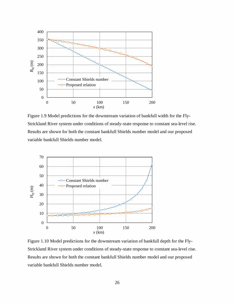
the case of constant bankfull Shields number, the bankfull depth increased from 7.38 m to 62.9

m over 200 km of channel, equivalent to an unrealistic 850% increase (Figure 1.10); the majority

of this change occurs over the last quarter length of the channel as depth increases. Our

proposed formulation with variable bankfull Shields number shows a more muted increase in

bankfull depth, from 7.46 m at the upstream end to 15.8 m at the outlet. Both cases are shown in

Figure 1.10.

15

Bankfull width linearly decreases by 88% (360.2 m to 42.2 m) in the constant bankfull

Shields number formulation, but non-linearly decreases only by 53% (355.7 m to 189.1 m) with

the proposed variable Shields number formulation (Figure 1.9). Corresponding widths extracted

from the most recent Google Earth image are 420 m and 300 m, corresponding to a 29%

decrease (Table 1.2). Both cases are shown in Figure 1.9. The variable Shields number

formulation is clearly more in accord with the data. A major part of the discrepancy between the

observed percentage width decrease and that predicted by our proposed model is likely due to the

fact that the model results assume constant sea level rise of 10 mm/year, whereas in reality the

rate of sea level rise had changed in time.

The differences in slope and bed elevation profile predicted by the two models are

relatively weak, but still evident (Figure 1.11 and Figure 1.12). The proposed relation results

show a meter or more difference in bed elevation between the two models over the first 100 km

of studied reach. Previous results using the constant bankfull Shields number model paired with

Exner equation gave adequate values for bed elevation (Parker et al. 2008), but unrealistically

strong downstream variation in width and depth.

Figure 1.13 and Figure 1.14 plot the results for both models over observed data of Figure

1.2 and Figure 1.7, respectively. Figure 1.13 shows the upstream (reference) and downstream

values of τ*bf / S

0.53 versus dimensionless grain size D*, and Figure 1.14 shows the upstream

(reference) and downstream values of Cz against the corresponding values for bed slope S. In the

case of constant bankfull Shields number τ*bf remains constant. In the case of our proposed

variable bankfull Shields number model, τ*bf increases downstream, the upstream value is at the

middle of the scatter of the data, and the downstream value is only slightly outside of it. In the

case of Cz, the results of our model follow the trend of the data, whereas the constant Shield

stress model does not. In both figures, however, the values for both models fit within the scatter

of the data.

1.8 DISCUSSION: APPLICATION TO MODERN SEA LEVEL RISE DRIVEN BY CLIMATE

CHANGE

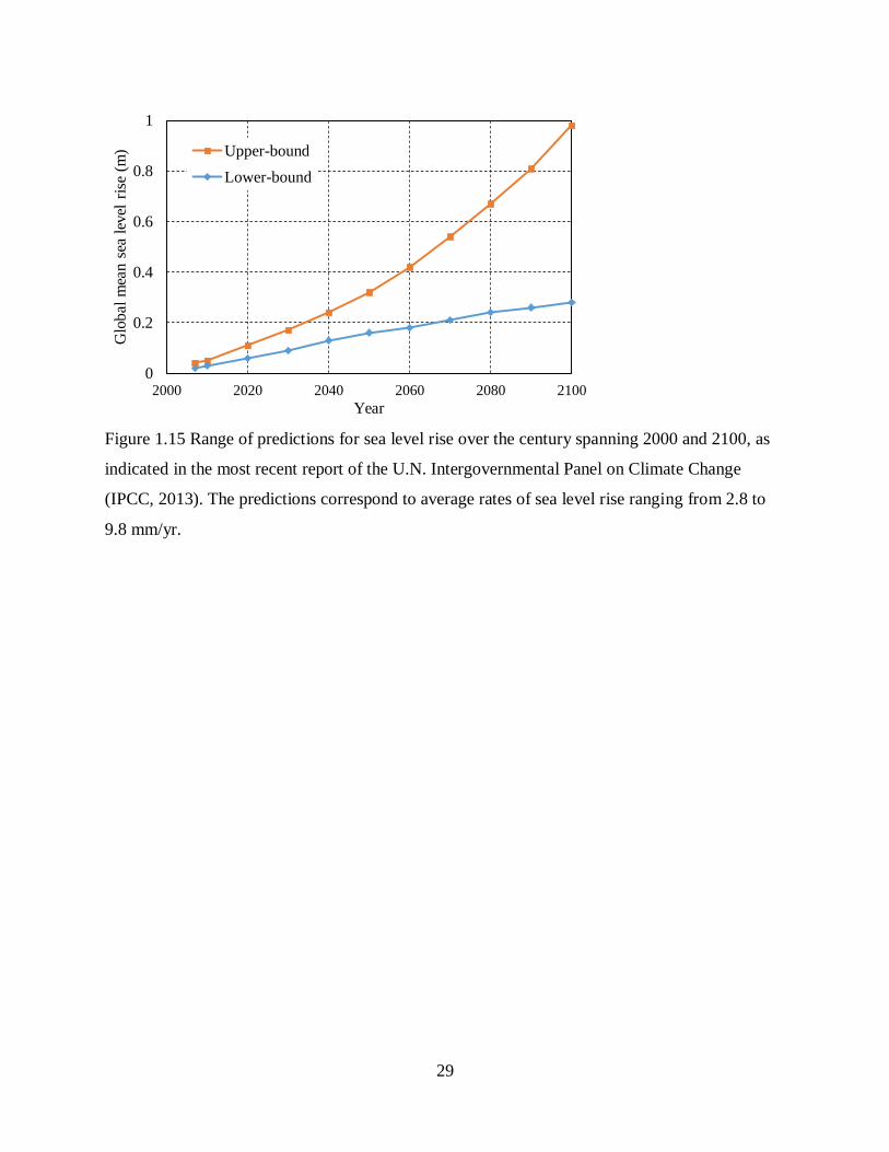
The model presented here has direct application to modern sea level rise associated with

climate change. Figure 1.15 shows the range of predictions for sea level rise over the century

16

from 2000 to 2100, as specified in the U.N. Intergovernmental Panel on Climate Change (IPCC,

2013). The indicated values correspond to average rates of sea level rise ranging from 2.8 to 9.8

mm/yr. Our proposed variable Shields number model, applied in the context of Parker et al.

(2008) for which a river ends in a delta, is directly applicable to the prediction of the response of

river profiles to modern sea level rise. Indeed, the high end of sea level rise nearly equals to rate

10 mm/yr used herein for the case of the Fly-Strickland River system.

Certain of the results obtained in Section 6 deserve emphasis. In the constant Shields

number formulation, slope is independent of grain size, whereas in our proposed formulation

slope strongly increases with grain size. We speculate that the latter result is more reasonable. In

the constant Shields number formulation, bankfull width is independent of bankfull discharge,

whereas in our proposed formulation bankfull width increases strongly with bankfull discharge.

Again, we speculate that the latter result is more reasonable.

In the present application of the model, grain size D is held constant at 0.25 mm. In

reality, however, large sand-bed rivers typically show a tendency for downstream fining of grain

size, which may result in a somewhat stronger increase of the bankfull Shields number and in a

better prediction of the streamwise changes in bankfull channel geometry. In order to account for

this effect, it is necessary to consider a grain size mixture and allow for selective deposition. The

methodology for this is specified in Wright and Parker (2005).

1.9 CONCLUSIONS

Previous relations for the dependency of bankfull width, bankfull depth and bed slope

have been based on the assumption of constant formative bankfull Shields number. Here we

show that this assumption does not adequately represent the data. We propose a new relation for

which bankfull formative Shields number is a variable. The implications of our proposed

relation are as follows.

Empirical analysis of measured data from natural rivers show that the bankfull, or

formative Shields number can be accurately described as a universal function of slope

and grain size than by a constant value. This function was determined from a data base

including 230 river reaches, with bankfull discharge varying from 0.34 to 216,340 m3/s,

17

bankfull width varying from 2.3 to 3 400 m, bankfull depth varying from 0.22 to 48.1 m,

bed slope varying from 8.810-6 to 5.2 10-2, and characteristic bed grain size varying

from 0.04 to 168 mm.

This relation gives the unexpected result that when bankfull shear velocity and bankfull

depth are computed from the relation for bankfull Shields number, they are dependent on

kinematic viscosity of water but independent of bed material grain size.

The dependence of bankfull shear velocity on viscosity may be due to the presence of

fine-grained suspended sediment load in the system, the characteristic grain size of which

is not represented by the characteristic grain size of the bed material. The fall velocity of

fine sand and silt is strongly dependent on viscosity, and it is from this material that much

of the floodplain is constructed.

Bed material grain size, does, however, enter in the predictive relations for bankfull

depth, bankfull width and bed slope as functions of bankfull discharge and bankfull total

bed material load.

The proposed relation for bankfull Shields number can be implemented into a model for

the long profiles of bankfull width, bankfull depth, bed slope and bed elevation self-

formed channels using, relations derived from: a) our proposed empirical relation for

bankfull Shields number, which varies with slope and grain size, b) momentum balance,

c) continuity, d) a relation for resistance coefficient, and d) a bed material load transport

relation.

Models using the constant bankfull Shields number formulation, applied to the case

constant sea level rise at a rate of 10 mm/yr associated with Holocene deglaciation,

predict long profiles for which bankfull depth and width increase unrealistically in the

downstream direction. A more reasonable pattern is predicted from our proposed variable

bankfull Shields number formulation.

Our new model is directly applicable to the prediction of river response to modern sea

level rise associated with climate change. Predicted rates of sea level rise range from 2.8

to 9.8 mm/yr, the upper bound corresponding to the case modeled here.

18

Table 1.1 Fly-Strickland River system model parameters, from Parker et al. (2008)

Parameter Value Units Descriptions

Qbf 5 700 m3/s Bankfull water discharge

If 0.175 - Flood intermittency

Qtbff 0.80 m3/s Sand feed rate during floods

Λ 1.0 - Mud/sand deposition ratio

Ω 2.0 - Channel sinuosity

D 0.25 mm Characteristic sand grain size

Bf 12 000 m Floodplain width

λp 0.35 - Porosity of channel/floodplain complex

R 1.65 - Submerged specific gravity of sediment

ξd 10 mm/yr Rate of sea-level rise

SR 0.0001 m/m Reference slope at sand-gravel transition

τ*R 1.82 - Reference bankfull Shields number

CzR 25 - Reference Chezy friction factor

Table 1.2 Measurements of bankfull channel widths (in kilometers) of the Fly-Strickland River

system, at the gravel-bed transition and just upstream of Everill Junction, from 4/9/2013 Google

Earth Landsat image

Measurement Gravel-sand transition (km) Just upstream of Everill Junction (km)

1 0.48 0.32

2 0.41 0.33

3 0.38 0.28

4 0.42 0.28

5 0.3

Average 0.4225 0.302

19

Figure 1.1 Bankfull Shields number τ*bf versus a) dimensionless grain size D*; and b) bed slope S

for rivers ranging from silt-bed to cobble-bed. The data are stratified into five grain size ranges.

Note that τ*bf increases with slope for every grain size range. Also shown in a) are lines denoting

the onset of bed motion and the onset of significant sediment suspension.

0.001

0.01

0.1

1

10

100

1 10 100 1000 10000

τ*bf

D*

Mostly suspension

No motion

Mostly bedload

(a)

0.0625mm

0.5 mm2 mm

16 mm

0.001

0.01

0.1

1

10

100

1.E-6 1.E-5 1.E-4 1.E-3 1.E-2 1.E-1

τ*bf

S

(b)

20

Figure 1.2 Similarity collapse for τ*bf /S0.53 versus D*. The regression relation, i.e. Eq. (1.5), is

shown in the plot.

τ*bf/S

0.53 = 1220(D*)-1

R² = 0.948

1E-1

1E+0

1E+1

1E+2

1E+3

1E+4

1 10 100 1000 10000

τ*bf/S

0.53

D

0.04 - 168 mm

Regression line fit

21

Figure 1.3 a) Dimensionless bankfull depth H*bf = Hbfg1/3 / (R)2/3 and; b) dimensionless

bankfull shear velocity u*bf = u*bf / (Rgν)1/3 versus bed slope. The dashed lines represent direct

power-law fit of the data. The solid lines represent the relations described by Eqs. (1.7a, b), also

displayed on the plots.

1.E+3

1.E+4

1.E+5

1.E+6

1.E-6 1.E-5 1.E-4 1.E-3 1.E-2 1.E-1

H*bf

S

(a)

H*bf = 1220S-0.47

1

10

100

1.E-6 1.E-5 1.E-4 1.E-3 1.E-2 1.E-1

u*bf

S

< 0.0625 mm 0.0625 - 0.5 mm 0.5 - 2 mm

2 - 25 mm >25 mm Analysis

Direct regression

(b)

ũ*bf = 35.0S0.26

22

Figure 1.4 a) Similarity collapse for τ*

bf / S0.53 versus D*, including the dataset of Hey and

Thorne (1986). Types I – IV represent the four classes of bank and floodplain vegetation density,

with Type I having the lowest bank height and least floodplain vegetation density, and Type IV

having the highest bank height and greatest floodplain vegetation density. The solid line

represent Eq. (1.5) and; b) expanded view of Figure 1.4a.

1E-1

1E+0

1E+1

1E+2

1E+3

1E+4

1 10 100 1000 10000

τbf/S0.53

D

Compendium

Type I, D > 25 mm

Type II, D > 25 mm

Type III, D > 25 mm

Type IV, D > 25 mm

Type I, D < 25 mm

Type II, D < 25 mm

Type III, D < 25 mm

Type IV, D < 25 mm

Equation (1.5)

(a)

0.1

1

10

100 1000 10000

τbf/S0.53

D

Type I, D > 25 mm

Type II, D > 25 mm

Type III, D > 25 mm

Type IV, D > 25 mm

Type I, D < 25 mm

Type II, D < 25 mm

Type III, D < 25 mm

Type IV, D < 25 mm

Equation (1.5)

(b)

23

Figure 1.5 a) Dimensionless bankfull depth H*bf = Hbfg

1/3 / (R)2/3, including the dataset of Hey

and Thorne (1986). Types I – IV represent the four classes of bank and floodplain vegetation

density, with Type I having the lowest bank height and least floodplain vegetation density, and

Type IV having the highest bank height and greatest floodplain vegetation density, and; b)

dimensionless bankfull shear velocity u*bf = u*bf / (Rgν)1/3 versus bed slope, also including the

dataset of Hey and Thorne (1986). The solid lines represent the relations described by Eqs. (1.7a,

b), also displayed on the plots.

1E+3

1E+4

1E+5

1E+6

1E-6 1E-5 1E-4 1E-3 1E-2 1E-1 1E+0

H*bf

S

Compendium

Type I, D > 25 mm

Type II, D > 25 mm

Type III, D > 25 mm

Type IV, D > 25 mm

Type I, D < 25 mm

Type II, D < 25 mm

Type III, D < 25 mm

Type IV, D < 25 mm

Equation (1.7b)

1

10

100

1E-6 1E-5 1E-4 1E-3 1E-2 1E-1 1E+0

u*bf

S

Compendium

Type I, D > 25 mm

Type II, D > 25 mm

Type III, D > 25 mm

Type IV, D > 25 mm

Type I, D < 25 mm

Type II, D < 25 mm

Type III, D < 25 mm

Type IV, D < 25 mm

Equation (1.7a)

24

Figure 1.6 Dimensionless fall velocity Rf = vs/(RgD)1/2 versus dimensionless grain size D* =

(Rg)1/3Dk/2/3, from the relation of Dietrich (1982). The points represent values of Rf,bank

computed from the same relation, using the bank/floodplain grain sizes Dbank from Hey and

Thorne (1982).

Figure 1.7 Plot of dimensionless Chezy resistance coefficient Cz at bankfull flow versus slope S.

Data are shown for only two grain size ranges of Figure 1.1, and Figure 1.2, covering D – 0.0625

mm to 2 mm. i.e. very fine to medium sand. The regression relation shown in the figure, i.e. Eq.

(1.17), was obtained only using data for D – 0.0625 mm to 2 mm.

0.001

0.01

0.1

1

10

0.1 1 10 100 1000

Rf

D*

Type I

Type II

Type III

Type IV

Cz = 2.53S-0.19

R² = 0.25

1

10

100

1E-6 1E-5 1E-4 1E-3 1E-2 1E-1

Cz

S

0.0625 - 2 mm

25

Figure 1.8 Aerial view of the Fly-Strickland River system, from 1987-1994 NASA/USGS

Landsat TM data. The study reach extends from the gravel-bed transition to 200 km downstream.

0 50 100 150 20025

Kilometers ±

Middle

Fly River Strickland

River

Lower

Fly River

PAPUA

NEW GUINEA

Everill

Junction

Fly Estuary

Upper

Fly River

Ok Tedi

River

Gravel-sand

Transition

26

Figure 1.9 Model predictions for the downstream variation of bankfull width for the Fly-

Strickland River system under conditions of steady-state response to constant sea-level rise.

Results are shown for both the constant bankfull Shields number model and our proposed

variable bankfull Shields number model.

Figure 1.10 Model predictions for the downstream variation of bankfull depth for the Fly-

Strickland River system under conditions of steady-state response to constant sea-level rise.

Results are shown for both the constant bankfull Shields number model and our proposed

variable bankfull Shields number model.

0

50

100

150

200

250

300

350

400

0 50 100 150 200

Bb

f(m

)

x (km)

Constant Shields number

Proposed relation

0

10

20

30

40

50

60

70

0 50 100 150 200

Hb

f(m

)

x (km)

Constant Shields number

Proposed relation

27

Figure 1.11 Model predictions for the downstream variation of bed slope for the Fly-Strickland

River system under conditions of steady-state response to constant sea-level rise. Results are

shown for both the constant bankfull Shields number model and our proposed variable bankfull

Shields number model.

Figure 1.12 Model predictions for the downstream variation of deviatoric bed elevation for the

Fly-Strickland River system under conditions of steady-state response to constant sea-level rise.

Results are shown for both the constant bankfull Shields number model and our proposed

variable bankfull Shields number model.

0E+0

2E-5

4E-5

6E-5

8E-5

1E-4

1E-4

0 50 100 150 200

S

x (km)

Constant Shields number

Proposed relation

0

2

4

6

8

10

12

14

0 50 100 150 200

ηd

ev(m

)

x (km)

Constant Shields number

Proposed relation

28

Figure 1.13 Results of the steady-state model for Shields number subject to constant sea-level

rise, plotted with the data and regression line of Figure 1.2. The arrows show the reference

values of τ*bf at the upstream end of the reach, and the upstream and downstream values of τ*

bf in

the constant and our proposed variable bankfull Shields number models. The downstream value

for τ*bf for the proposed bankfull Shields stress model is the same as the upstream value.

Figure 1.14 Results of the steady-state model for Chezy friction coefficient Cz subject to

constant sea-level rise, plotted with the data and regression line of Figure 1.7. The arrows show

the reference values of Cz at the upstream end of the reach, and the downstream values predicted

by both the constant and variable bankfull Shields number models.

1E-1

1E+0

1E+1

1E+2

1E+3

1E+4

1 10 100 1000 10000

τbf/S0.53

D*

Natural rivers

Constant Shields number

Proposed relation

Fit to observed data

Reference values τR , SR

Upstream and downstream

values in proposed relation

Downstream, constant Shields numberUpstream, constant Shields number

1

10

100

1E-6 1E-5 1E-4 1E-3 1E-2 1E-1

Cz

S

Natural rivers

Constant Shields number

Proposed relation

Fit to observed data

Reference CzR

Upstream values

Downstream values

29

Figure 1.15 Range of predictions for sea level rise over the century spanning 2000 and 2100, as

indicated in the most recent report of the U.N. Intergovernmental Panel on Climate Change

(IPCC, 2013). The predictions correspond to average rates of sea level rise ranging from 2.8 to

9.8 mm/yr.

0

0.2

0.4

0.6

0.8

1

2000 2020 2040 2060 2080 2100

Glo

bal

mea

n s

ea l

evel

ris

e (m

)

Year

Upper-bound

Lower-bound

30

CHAPTER 2

RESPONSE OF THE MINNESOTA RIVER TO VARIANT SEDIMENT LOADING

2.1 INTRODUCTION

The Minnesota River is a major river in the state of Minnesota and a tributary of the

Mississippi River. At 540 kilometers in length, the Minnesota River drains an area of

approximately 43 430 square kilometers, which contains 13 major watersheds and parts or all of

38 counties (Musser et al. 2009). Sediment in the Minnesota River has a significant impact on

the river itself and rivers and water bodies downstream - coring studies in Lake Pepin, a natural

lake approximately 80 kilometers downstream of the confluence of the Minnesota and

Mississippi River, indicate a near 10-fold increase in sedimentations rates in the lake during the

past 150 years (Engstrom et al. 2009), 80% - 90% of which come from the Minnesota River

(Engstrom et al. 2009, Kelley et al. 2006). This is especially notable by the fact that the

Minnesota River Basin contributes only a third of the area drained by Lake Pepin (Engstrom et

al. 2009, Kelley et al. 2006). The relatively high rate of sediment yield from the Minnesota River

is of environmental concern since sediments and turbidity are major pollutants to U.S. streams

(USEPA 2014). Other concerns include, for example, the volume loss of Lake Pepin. It is

projected at 1990s rate of sedimentation that the volume of Lake Pepin would be reduced to 0 in

about 340 years (Engstrom et al. 2009).

2.2 STUDY AREA

In this paper, we examine via numerical modeling the effects of variable sediment

loading on the Minnesota River. In particular, we focus on the reach of the Minnesota River

downstream of the city of Mankato (Figure 2.1). Five major watersheds, the Middle Minnesota,

Lower Minnesota, Watonwan, Blue Earth, and Le Sueur drain into the Minnesota River

downstream of Mankato. These areas are joined by all the drained area upstream of Mankato to

give the total drainage of the Minnesota River. It is worth noting that the Le Sueur watershed,

although only having 6.6% of Minnesota River Basin’s area, contributes 30% of the Minnesota

River sediment load, the most of any Minnesota River tributary (Wilcock 2009).

31

2.3 METHOD

Model Formulation

For the purpose of this study, we have developed a one-dimensional numerical model of

coupled water flow, sediment transport, and channel bed/floodplain morphodyanmics. The

governing equations and simplifications of this model are as follows. The river is assumed to be

at bankfull flow for a fraction of each year, If, and with no flow for the remainder. If, which

denotes the fraction of each year in which the river is morphologically active, is called flood

intermittency. Furthermore, flow is assumed to be steady and uniform. Thus, the Chezy

resistance relation can be used to compute the bankfull water depth, Hbf :

1/32

bf f

bf

q CH

gS

, (2.1)

where qbf is the bankfull water discharge per unit channel width, g is the acceleration of gravity,

S is the channel bed slope, and Cf is the friction coefficient, related to the dimensionless Chezy

coefficient, Cz, by

2

fC Cz . (2.2)

Sediment is grouped into 1) bed material load and 2) wash load, where bed material load

is taken to represent sediment sizes > 0.0625 mm (sand) and wash load represents sediment sizes

< 0.0625 mm (mud). Wash load is assumed to entirely suspended in the water column. Thus, the

transport of wash load (at bankfull), Qwbf, is governed only by water discharge, i.e.

b

wbf bfQ aQ , (2.3)

where Qbf is the bankfull water discharge, and a and b are each an appropriate coefficient and

exponent determined from field data.

The bed material load contains bedload and suspended load of bed material (sediment

size greater than 0.0625 mm). The Engelund-Hansen (Engelund and Hansen 1967) transport

relation for sand-bed rivers is used herein:

2.50.05tbf bf

f

q RgDDC

, (2.4)

32

where qtbf is the bankfull bed material load per unit channel width, α is an adjustment factor for

the specific modeled reach, R is the submerged specific gravity of sediment, D is a characteristic

grain size, and *bf is the bankfull Shields number, computed (for steady, uniform flow) as

bf

bf

H S

RD . (2.5)

We assume that sediment is transported in-channel but is deposited across the entire

channel/floodplain complex. In addition, the deposition of mud follows a fix ratio to the

deposition of sand. Thus, the channel bed/floodplain morphodynamics is governed by

1

1

f tbf

fp

I dqd B

dt B dx

, (2.6)

where is the average channel bed/floodplain elevation, t is time, If is the flood intermittency

factor, is channel sinuosity, is the mud to sand deposition ratio, B is channel width, Bf is

floodplain width, and x is down-channel distance.

Equation (2.6) requires a numerical solution. To achieve this, we employ the finite

volume method (FVM) for its mass conservative properties. Figure 2.2 shows a schematic of the

computational scheme. Mass conservation is achieved by calculating sediment load in between

computational nodes (for floodplain/bed elevation).

Model Parameters

Table 1.1 lists the required model input parameters and their descriptions. The model

parameters are obtained as follows. The Engelund-Hansen adjustment factor, α, can be obtained

by

, , , ,/t field mean t EH meanQ Q , (2.7)

where Qt,field,mean is the observed bed material load from the field, averaged across the entire

range of flows and Qt,EH,mean is the bed material load, averaged across the entire range of flows,

computed by the Engelund-Hansen relation. Essentially, the adjustment factor accounts for the

difference between sediment load computed from Engelund-Hansen and that from the field.

Qt,field,mean can be computed by

33

, , ,

1

n

t field mean i t i

i

Q p Q

, (2.8)

where i is the index of each water discharge, n is the total number of observed discharges, pi is

the probability of occurrence of each discharge, and Qt,i is the bed material load at each

discharge, obtained by

, , , ,t i s i sand i b iQ Q f Q , (2.9)

where Qs,i is the total suspended load (including both bed material and wash load) at each

discharge, fsand,i is the fraction of bed material in total suspended load at each discharge, and Qb,i

is bedload at each discharge.

We obtain pi from discharge data of USGS gauging station at Mankato (upstream end of

study reach) for period June 1, 1903 to Feb. 15, 2014. Figure 2.3 shows the flow duration curve

created from this data. To find Qs,i, we use a relation of Qs,i as a function water discharge (Qi)

obtained from USGS suspended sediment data at Mankato (Figure 2.4, period of Oct. 1, 1967 to

Sep. 30, 2012). We compute fsand,i = 1 - fmud,i, where fmud,i is the fraction of washload in

suspended load, which is a function of Qi, obtained from the same data as we used for Qs,i

(Figure 2.5). For computation of Qb,i, we use data from a recent bedload sampling program at

USGS, again at Mankato (Figure 2.6, period Oct. 1, 1967 to Sep. 30, 2012, source: Christopher

Ellison, USGS). With these relations, we find Qt,field,mean = 0.217 megatons/year (Mt/year).

Qt,EH,mean, or the bed material load averaged across the entire range of flows, can be

computed from the standard Engelund-Hansen relation, summed across all flows:

2.5

, ,

1

0.05n

t EH mean i i i

i f

Q p B RgDDC

, (2.10)

where Bi is the top width for each discharge, and *i, the Shields number for each discharge, is

computed by

* ii

H S

RD , (2.11)

where Hi is the mean water depth at each discharge. The determination of Bi and Hi requires a

representative channel geometry. The channel geometry near Mankato (Figure 2.7, USACE,

circa 1970s) however, is not truly representative of the study reach, since channel in this location

is highly engineered and has unusually high banks. This complication can also be seen in the

stage-discharge data at Mankato (Figure 2.8). It is difficult to identify a bankfull discharge from

34

this stage-discharge data since there is no clear rollover to indicate the threshold of overbank

flow.

We use instead the channel geometry near Jordan (located near mid-reach in our modeled

reach, Figure 2.9) as our representative channel geometry. We estimate, from the stage-discharge

relation (Figure 2.10), a bankfull discharge of 600 m3/s. Channel width (Figure 2.11) and channel

width data (Figure 1.12) shows agreement with our estimated bankfull discharge. We remove

several data points that show unusually high widths compared against values calculated from the

USACE channel-cross section (Figure 2.13). With the remaining data, we obtain relations of

Bi/Bbf (Figure 2.14) and Hi/Hbf (Figure 2.15).

In further calcuations, we take Qbf = 570 m3/s (bankfull discharge), Bbf = 105 m (bankfull

width), Hbf = 4.68 m (bankfull depth). These are used because they are surveyed values near

Mankato, from Johannesson et al. (1988). Median grain size of bed material 0.6 mm at Mankato

(Figure 2.16) is used as the characteristic sediment size D. Figure 2.17 and Figure 2.18 show that

the values of Qbf, Bbf, Hbf, S, and D at Mankato are consistent with the trends seen in 230 reaches

in Li et al. (accepted), which covers a wide range of Qbf, Bbf, Hbf, S, and D. We obtain Cz = 15

(dimensionless Chezy coefficient) from examination of field data of Cz at Mankato (Figure

2.19), Jordan (Figure 2.20), and Fort Snelling (Figure 2.21).

Figure 2.22 shows riverbank and bluff elevation profiles of the Minnesota River between

Mankato and its confluence with the Mississippi River. A distinct break in slope can be observed

in both the left and right riverbanks at mid-reach. The average slope of the banks is 0.00022 in

the upper reach (upper 80 km) and 0.000053 in the lower reach (lower 80 km). In our

calculations of model parameters given below, we use the average slope of the upper reach

(0.00022) since it is more representative of conditions near Mankato. Using data and relations

described in this section, we find the observed bed material load averaged across all flows,

defined by Eq. (2.8), Qt,field,mean = 0.217 Mt/year, and the Engelund-Hansen counterpart, defined

by Eq. (2.10), Qt,EH,mean = 1.079 Mt/year. Thus, we find, by Eq. (2.7), that the Engelund-Hansen

adjustment factor α = 0.201.

The flood intermittency factor, If, can be obtained by

, , , ,/f t EH mean t EH bankfullI Q Q , (2.12)

where Qt,EH,mean is previously defined in Eq. (2.10). Qt,EH,bankfull is Englund-Hansen bed material

load at bankfull conditions,

35

2.5

, ,

0.05t EH bankfull bf bf

f

Q B RgDDC

. (2.13)

All the required parameters to obtain Qt,EH,bankfull have already been discussed. We find

Qt,EH,bankfull = 4.163 Mt/year, thus If = 0.259.

In addition to the aforementioned model parameters, we take channel bed/floodplain

deposit porosity, p = 0.35 (assumed in the absence of field data); reach length L = 160 km

(measured from Landsat aerial photo); submerged specific gravity of sediment, R = 1.65 (for

quartz); floodplain width Bf = 1050 m (Landsat aerial photo); channel sinuosity = 2

(MacDonald et al. 1991); and mud/sand deposition ratio = 1 (assumed in the absence of field

data). Table 2.2 lists all model parameters with values and units.

Modeling Procedures

We perform the model simulation as follows:

1) Start with an assumed antecedent channel bed/floodplain slope for year 3190 BC (chosen

to be 5200 years before present). Sediment feed is set to 1/3.5 of present day sediment

load. Run for 5000 years (to 1810 AD). In this way we attempt to characterize antecedent

conditions before the advent of Old-World farming.

2) Continue the run (hot start) for 200 additional years (1810 to 2010) using present day

sediment load. In this way we attempt to capture the effect of Old World farming on

sediment production.

3) Reduce the load by half (from present day value), and run for 400 more years (2010 to

2410). In this way we simulate the effect of better management practices on sediment

production.

The change in sediment load at 1810 accounts for the relatively lower sediment loading

prior to intensive agriculture, as reflected by the low rates of sedimentation in Lake Pepin. The

multiplier of 3.5 is an estimate. For example, Belmont et al. (2011) estimates sediment output

from the Le Sueur River during period 2000 – 2010 to be about 4 times the average of the

Holocene (past 11700 years). A reduction in sediment load is applied at year 2010 to examine

the effects of reducing sediment input on the system.

36

2.4 RESULTS AND DISCUSSION

Figure 2.23 shows the simulation average channel bed/floodplain elevation profile in

years 3190 BC, 1810 AD, and 2010 AD. For comparison, the plot also includes the present-day

observed right channel-bank elevation. The simulation shown in Figure 2.23 uses an antecedent

bed/floodplain slope (in year 3190 BC) of 0.000053, corresponding to the average present-day

channel-bank slope of the lower reach (lower 80 km). Figure 2.24 and Figure 2.25 show the

same information as Figure 2.23, but for antecedent slopes of 0.00007 and 0.00008, respectively.

The simulated average channel bed/floodplain elevation compares reasonably well to the

observed values. They do, however, tend to underestimate the elevation of the upper reach

(upper 80 km) and overestimate the lower reach (lower 80 km). One major cause of this

discrepancy is likely the effects of downstream grain-size fining in the field. The simulations

only use a single representative grain-size.

Figure 2.26 shows the simulation elevation profiles in years 2010, 2210, and 2410 under

present sediment load and half of present sediment load. Figure 2.27 shows the change elevation

in years 2210 and 2410 from year 2010. It is clear that elevation changes are noticeably lower

under reduced sediment loading, especially in the upper quarter of the reach.

Figure 2.28 shows the percentage of bed material and wash load at the output of the reach

in year 1810. It is seen that the sediment output is predominantly (80.92%) wash load. Figure

2.29 shows the percentage of deposition versus output in bed material and wash load. It is seen

that a much greater portion of wash load (87.4%) is sent as output than bed material (62.06%).

Figure 2.30 and Figure 2.31 show sediment output and deposition over the entire

simulation period (3190 BC – 2410 AD), with for bed material load and wash load shown

separately. A few observations can be made. First, it is evident again that the output of bed

material load is less than that of wash load over the entire period. Second, output of bed material

changes very little in year 1810, when sediment input is increased by a factor of 3.5. In fact,

sediment output just begins to slightly increase in year 2010, 200 years after the change in

sediment input. Output of wash load, on the other hand, shows an immediate and significant

change when input is increased in 1810. It again changes immediately and significantly when

sediment input is reduced in year 2010. This tremendous difference between the behaviors of bed

37

material and wash load is due to the relatively high mobility of wash load compared to bed

material load.

To better understand the movement of bed material load in the system, we show in Figure

2.32, Figure 2.33, and Figure 2.34 the deposition rates (equal for bed material and wash load) in

four quarter-subreaches, from upstream to downstream. It is worth noting that as far as

deposition rates are concerned, out of all the subreaches, only the most downstream has a direct

effect on sediment output. The proportion of sediment deposition in the first quarter length of the

reach decreases in the period from 3190 BC to 1810 AD, while sediment deposition in the other

three quarters increase during the same period (Figure 2.32). However, the proportion of

sediment deposition in the last quarter is much lower than the other three. During the period

1810 – 2010, sediment deposition predominantly occurs in the first quarter of the reach. The

second half registers a very small fraction of deposition and little to none is seen in the last

quarter (Figure 2.33). During 2010 – 2410, although considerable sediment deposition is seen in

each of the first three quarters of the reach, the last quarter again receives a much smaller

portion, with very little increase in the 400 year period (Figure 2.34).

Figure 2.35, Figure 2.36, and Figure 2.37 show similar information as Figure 2.32, Figure

2.33, and Figure 2.34, but using much smaller subreaches (2.67 km). It can be seen that the

propagation of deposition rates through the system is similar to a diffusion process, with all of

the change in input initially concentrated at the most upstream, but with gradual spreading

downstream throughout the reach. Figure 2.35 shows that by 690 BC, deposition due to change

in sediment input in 3190 BC has reached the downstream end. However, deposition due to

change in sediment input in 1810 has only reached about mid-reach (80 km) in 2010 (after 200

years, Figure 2.36). This signal has just reached the downstream end in 2410 (after 600 years,

Figure 2.37). This explains the behavior of the bed material output seen in Figure 2.30, that is,

bed material moves simply too slowly for any significant change in output to occur 600 years

after a change in the input. This is a very different behavior as compared to mud load, where

output changes immediately in response to changed input.

The results of this study, in particular the composition of sediment load (i.e. percentage

bed material versus wash load) and the time rate of change of sediment output for bed material

and wash load, show that wash load has a much more significant impact (both in magnitude and

time of response) on sediment output from the Minnesota River. Thus, strategies to manage

38

sediment delivery from the Minnesota River to the Mississippi River should focus primarily on

controlling sediment input of wash load (mud), rather than bed material load (sand). Specifically,

any changes in the bed material input are not likely to have an effect on sediment output in the

next 600 years. However, any changes in wash load input will have a near-immediate impact on

sediment output.

39

Table 2.1 List of required model input parameters and their descriptions.

Parameter Description

Qbf Bankfull water discharge

If Flood intermittency factor

D Characteristic sediment size

p Channel bed/floodplain porosity

Sa Antecedent average channel bed/floodplain slope

Qbff Bed material feed rate

L Reach length

Cz Dimensionless Chezy coefficient

α Engelund-Hansen adjustment factor

R Submerged specific gravity of sediment

Bf Floodplain width

Channel sinuosity

Mud/sand deposition ratio

40

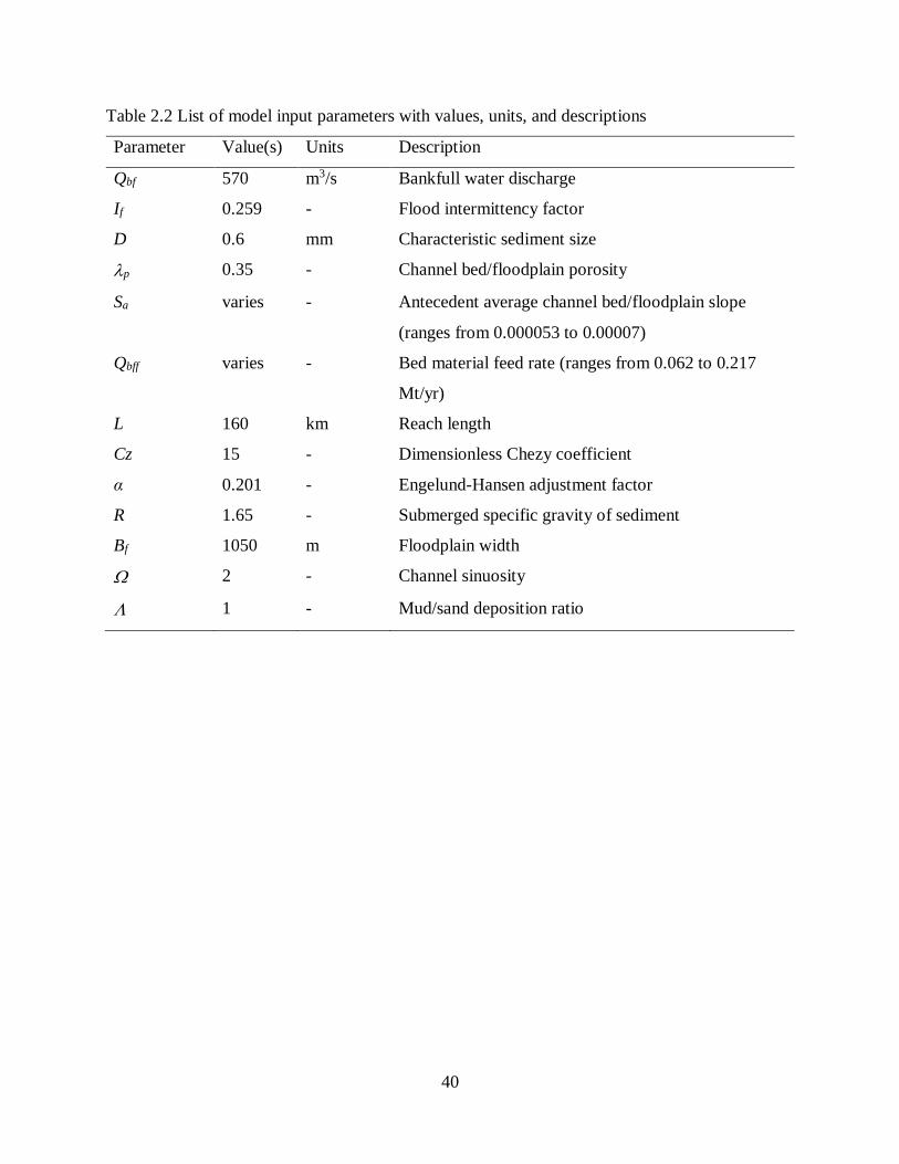
Table 2.2 List of model input parameters with values, units, and descriptions

Parameter Value(s) Units Description

Qbf 570 m3/s Bankfull water discharge

If 0.259 - Flood intermittency factor

D 0.6 mm Characteristic sediment size

p 0.35 - Channel bed/floodplain porosity

Sa varies - Antecedent average channel bed/floodplain slope

(ranges from 0.000053 to 0.00007)

Qbff varies - Bed material feed rate (ranges from 0.062 to 0.217

Mt/yr)

L 160 km Reach length

Cz 15 - Dimensionless Chezy coefficient

α 0.201 - Engelund-Hansen adjustment factor

R 1.65 - Submerged specific gravity of sediment

Bf 1050 m Floodplain width

2 - Channel sinuosity

1 - Mud/sand deposition ratio

41

Figure 2.1 Overview of the study area. The modeled reach begins at the city of Mankato and

ends at the Minnesota-Mississippi confluence. Each different colored area shows a different

watershed. Aerial imagery from NASA Blue Marble Next Generation. River and watershed

delineations from the USGS National Hydrography Dataset.

42

Figure 2.2 Outline of the finite volume computational scheme used to solve the morphodynamics

equation [Eq. (2.6)]. Solid dots represent computational nodes. Also represents average

floodplain/channel bed elevation, qtbf represents bed material load per unit width and dx is the

grid size.

Figure 2.3 Flow duration curve of the Minnesota River at Mankato, period of June 1, 1903 to

Feb. 15, 2014. Data from USGS National Water Information System.

0.1

1

10

100

1000

10000

0.001 0.01 0.1 1 10 100

Wat

er d

isch

arge

(m3/s

)

Percent of time exceeded (%)

Mankato

1903-2014

43

Figure 2.4 Plot of total suspended load versus discharge at Mankato, for period Oct. 1, 1967 to

Sep. 30, 2012. Data from USGS National Water Information System.

Figure 2.5 Plot of percent washload in suspended load versus discharge at Mankato, for period

Oct. 1, 1967 to Sep. 30, 2012. Data from USGS National Water Information System.

Qs,i = 2.4257Qi1.3825

R² = 0.9099

1E+0

1E+1

1E+2

1E+3

1E+4

1E+5

1E+6

1 10 100 1000 10000

Su

sp s

edim

ent

load

(to

ns/

day

)

Discharge (m3/s)

Mankato

fmud,i = (-0.0122Qi + 85.093)/100

R² = 0.1303

0

20

40

60

80

100

0 500 1000 1500 2000

% w

ashlo

ad i

n s

usp

ended

lo

ad

Discharge (m3/s)

Mankato

44

Figure 2.6 Plot of bedload versus discharge at Mankato, for period Mar. 14, 2012 to Apr. 25,

2013. Data provided by Christopher Ellison of USGS.

Figure 2.7 Minnesota River channel cross-section at Mankato. Data from USACE, circa 1970s.

As can be inferred from the plot, the river is channelized and leveed at this location.

Qb,i = 0.2065Qi1.2603

R² = 0.5146

0.1

1

10

100

1000

10000

1 10 100 1000

Bed

load

(to

ns/

day

)

Discharge (m3/s)

Mankato

226

230

234

238

242

246

250

540 580 620 660 700

Ele

vat

ion (

m)

Station (m)

Mankato

45

Figure 2.8 Plot of USGS gage height versus discharge at Mankato, for period Apr. 9, 1951 to

Jan. 1, 2014. Data from USGS National Water Information System.

0

2

4

6

8

10

0 500 1000 1500 2000 2500 3000

Gag

e hei

ght

(m)

Discharge (m3/s)

Mankato

46

Figure 2.9 Cross-sectional geometry at Jordan for (a) entire valley and (b) channel portion only.

From USACE, circa 1970. Data from USGS National Water Information System.

205

210

215

220

225

230

3000 3300 3600 3900 4200 4500 4800 5100

Ele

vat

ion (

m)

Station (m)

Jordan(a)

206

208

210

212

214

216

218

220

4350 4370 4390 4410 4430 4450 4470

Ele

vat

ion (

m)

Station (m)

Jordan(b)

47

Figure 2.10 Plot of USGS gage height versus discharge at Jordan, for period Oct. 23, 1968 to

Jan. 30, 2014 (field measurements) and Oct. 2, 2009 to May 4, 2014 (gage measurements). Data

from USGS National Water Information System. Also shown is the estimated bankfull discharge

of 600 m3/s.

Figure 2.11 Plot of channel width versus discharge at Jordan, for period Oct. 23, 1968 to Jan. 1,

2014. Data from USGS National Water Information System. Also shown is the estimated

bankfull discharge at 600 m3/s.

0

2

4

6

8

10

12

0 500 1000 1500 2000 2500 3000

Gag

e hei

ght

(m)

Discharge (m3/s)

Jordan

2009-2014 Gage

1968-2014 Field

Bankfull discharge, 600 cms

0

400

800

1200

1600

0 500 1000 1500 2000 2500 3000

Chan

nel

wid

th (

m)

Discharge (m3/s)

Jordan

Bankfull discharge

600 cms

48

Figure 2.12 Plot of mean channel depth versus discharge at Jordan, for period Oct. 23, 1968 to

Jan. 1, 2014. Data from USGS National Water Information System. Also shown is the estimated

bankfull discharge of 600 m3/s.

Figure 2.13 Plot of channel width versus mean channel depth at Jordan, for period Oct. 23, 1968

to Jan. 1, 2014. Data from USGS National Water Information System. Also shown are values

computed from the USACE channel cross-section at Jordan (Figure 2.9b). Field data with

unreasonably high widths were removed.

0

2

4

6

8

10

0 500 1000 1500 2000 2500 3000

Mea

n c

han

nel

dep

th (

m)

Discharge (m3/s)

Jordan

Bankfull discharge

600 cms

0

30

60

90

120

0 1 2 3 4 5 6 7

Chan

nel

wid

th (

m)

Mean channel depth (m)

Jordan

Field kept

Field removed

Computed from USACE XS

49

Figure 2.14 Plot of Bi/Bbf versus Qi/Qbf, for period Oct. 23, 1968 to Jan. 1, 2014. Data from

USGS National Water Information System. Also shown are the same quantities computed from

the USACE channel cross-section at Jordan. The removed data points are the same as those in

Figure 2.13.

Figure 2.15 Plot of Hi/Hbf versus Qi/Qbf, for period Oct. 23, 1968 to Jan. 1, 2014. Data from

USGS National Water Information System. Also shown are the same quantities computed from

the USACE channel cross-section at Jordan. The removed data points are the same as those in

Figure 2.13.

0.1

1

0.01 0.1 1

Bi/B

bf

Qi/Qbf

Jordan

Field kept

Field removed

Computed from USACE XS

Bi/Bbf = Qi/Qbf0.15

0.1

1

0.01 0.1 1

Hi/H

bf

Qi/Qbf

Jordan

Field kept

Field removed

Computed from USACE XS

Hi/Hbf = Qi/Qbf0.35

50

Figure 2.16. Bed material grain size distribution at Mankato, for period Oct. 4, 1960 to Aug. 27,

2013. Data from USGS National Water Information System.

Figure 2.17 Plot of bankfull channel width (Bbf), bankfull mean channel depth (Hbf,) and bed

slope (S) versus bankfull discharge (Qbf), showing values at Mankato (red) and at 230 reaches

with a wide range of sediment sizes (blue) from Li et al. (accepted).

0

25

50

75

100

0.01 0.1 1 10 100

Per

cent

finer

(%

)

Grain size (mm)

Mankato

1E-6

1E-4

1E-2

1E+0

1E+2

1E+4

1E-1 1E+1 1E+3 1E+5 1E+7

Bankfull discharge, Qbf (m3/s)

Bbf m

Hbf m

S m/m

Hbf Mankato

S Mankato

Bbf Mankato

51

Figure 2.18 *bf/S0.53 versus D*, where is the bankfull Shields number, S is channel bed slope,

and D* = (Rg)1/3D/2/3, where R is the specific gravity of sediment, g is the acceleration of

gravity, is the kinematic viscosity of water, and D is the characteristic sediment size. Blue dots

show data from 230 reaches in Li et al. (accepted), and the red dot shows the value for Mankato.

Solid line shows the relation of the variable bankfull Shields number τ*bf/S0.53 = 1223(D*)-1 from

Li et al. (accepted).

Figure 2.19 Dimensionless Chezy coefficient (Cz) versus USGS gage height at Mankato, for

period Apr. 9, 1951 to Jan. 30, 2014. Data from USGS National Water Information System.

τ*bf/S0.53 = 1223(D*)-1

R² = 0.948

1E-1

1E+0

1E+1

1E+2

1E+3

1E+4

1 10 100 1000 10000

*bf/S0.53

D*

Compendium

Mankato

Li et al. (submitted)

0

10

20

30

0 2 4 6 8 10

Cz

Gage height (m)

Mankato

52

Figure 2.20 Dimensionless Chezy coefficient (Cz) versus USGS gage height at Jordan, for period

Oct. 23, 1968 to Jan. 30, 2014. Data form USGS National Water Information System.

Figure 2.21 Dimensionless Chezy coefficient (Cz) versus USGS gage height at Fort Snelling

(near end of model reach), for period Oct. 29, 1997 to Oct. 30, 2013. Data form USGS National

Water Information System.

0

5

10

15

20

25

0 2 4 6 8 10 12

Cz

Gage height (m)

Jordan

0

5

10

15

20

25

30

0 1 2 3 4 5 6 7

Cz

Gage height (m)

Fort Snelling

53

Figure 2.22 Elevation profiles of (a) left bank and left bluff and (b) right bank and right bluff of

the Minnesota River between Mankato and confluence of Minnesota and Mississippi Rivers.

Data from NASA Shuttle Radar Topography Mission.

0 40000 80000 120000

205

225

245

265

285

305

0 40000 80000 120000 160000

Down-valley distance (m)E

levat

ion (

m)

Down-channel distance (m)

Left bank

Left bluff

(a)

0 40000 80000 120000

205

225

245

265

285

305

0 40000 80000 120000 160000

Down-valley distance (m)

Ele

vat

ion (

m)

Down-channel distance (m)

Right bankRight bluff

(b)

54

Figure 2.23 Average channel bed/floodplain elevation profile from model output, for years 3190

BC, 1810 AD, and 2010 AD, starting with antecedent slope of 0.000053. Also shown (blue line)

is field measured present-day elevation profile of the right bank.

Figure 2.24 Average channel bed/floodplain elevation profile from model output, for years 3190

BC, 1810 AD, and 2010 AD, starting with antecedent slope of 0.00007. Also shown (blue line) is

field measured present-day elevation profile of the right bank.

205

210

215

220

225

230

235

240

0 40000 80000 120000 160000

Ele

vat

ion (

m)

Downstream distance (m)

Antecedent slope = 0.000053

3190 BC

1810 AD

2010 AD

Present right bank

205

210

215

220

225

230

235

240

0 40000 80000 120000 160000

Ele

vat

ion (

m)

Downstream distance (m)

Antecedent slope = 0.00007

3190 BC

1810 AD

2010 AD

Present right bank

55

Figure 2.25 Average channel bed/floodplain elevation profile from model output, for years 3190

BC, 1810 AD, and 2010 AD, starting with antecedent slope of 0.00008. Also shown (blue line) is

field measured present-day elevation profile of the right bank.

205

210

215

220

225

230

235

240

0 40000 80000 120000 160000

Ele

vat

ion (

m)

Downstream distance (m)

Antecedent slope = 0.00008

3190 BC

1810 AD

2010 AD

Present right bank

56

Figure 2.26 Average floodplain/channel bed elevation profile in years 2010, 2210, and 2410 with

(a) present upstream sediment load; and (b) half of present sediment load.

210

215

220

225

230

235

0 40000 80000 120000 160000

Ele

vat

ion (

m)

Downstream distance (m)

Present-day load 2010 AD

2210 AD

2410 AD

(a)

210

215

220

225

230

235

0 40000 80000 120000 160000

Ele

vat

ion (

m)

Downstream distance (m)

1/2 present-day load2010 AD

2210 AD

2410 AD

(b)

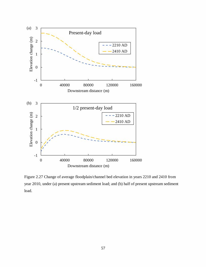
57

Figure 2.27 Change of average floodplain/channel bed elevation in years 2210 and 2410 from

year 2010, under (a) present upstream sediment load; and (b) half of present upstream sediment

load.

-1

0

1

2

3

0 40000 80000 120000 160000

Ele

vat

ion c

han

ge

(m)

Downstream distance (m)

Present-day load

2210 AD

2410 AD

(a)

-1

0

1

2

3

0 40000 80000 120000 160000

Ele

vat

ion c

han

ge

(m)

Downstream distance (m)

1/2 present-day load

2210 AD

2410 AD

(b)

58

Figure 2.28 Percentage of bed material (sand) and wash load (mud) at the output of the reach in

year 1810.

19.08%

80.92%

Sediment output,

1810 AD

Sand

Mud

59

Figure 2.29 Percentage of deposition and output for (a) bed material load (sand), and (b) wash

load (mud) in year 1810.

37.94%

62.06%

Sand,

1810 AD

Deposition

Output

(a)

12.60%

87.40%

Mud,

1810 AD

Deposition

Output

(b)

60

Figure 2.30 Bed material load (sand) output and deposition during the entire simulation period

(3190 BC – 2410 AD).

Figure 2.31 Wash load (mud) output and deposition during the entire simulation period (3190

BC – 2410 AD).

0

0.04

0.08

0.12

0.16

0.2

31

90

BC

19

40

BC

69

0 B

C

56

0 A

D

18

10

AD

Sed

imen

tati

on r

ate

(Mt/

yea

r) Sand

18

10

AD

18

50

18

90

19

30

19

70

20

10

20

10

20

90

21

70

22

50

23

30

24

10

Output

Deposition

0

0.1

0.2

0.3

0.4

0.5

31

90

BC

19

40

BC

69

0 B

C

56

0 A

D

18

10

AD

Sed

imen

tati

on r

ate

(Mt/

yea

r) Mud

1810 A

D

1850

1890

1930

1970

2010

2010

20

90

2170

22

50

23

30

24

10

Output

Deposition

61

Figure 2.32 Annual deposition rates (equal for bed material and wash load) by quarter

subreaches, for period of 3190 BC – 1810 AD. Note that the deposition rates are cumulative in

the vertical direction.

Figure 2.33 Annual deposition rates (equal for bed material and wash load) by quarter

subreaches, for period of 1810 – 2010. Note that the deposition rates are cumulative in the

vertical direction.

0

0.015

0.03

0.045

3190 BC 2190 BC 1190 BC 190 BC 810 AD 1810 AD

Dep

osi

tio

n r

ate

(Mt/

yea

r)

Year

Deposition rates

by subreach

First 1/4

First 1/2

First 3/4

All

0

0.06

0.12

0.18

1810 1850 1890 1930 1970 2010

Dep

osi

tio

n r

ate

(Mt/

yea

r)

Year

Deposition rates

by subreach

First 1/4

First 1/2

First 3/4

All

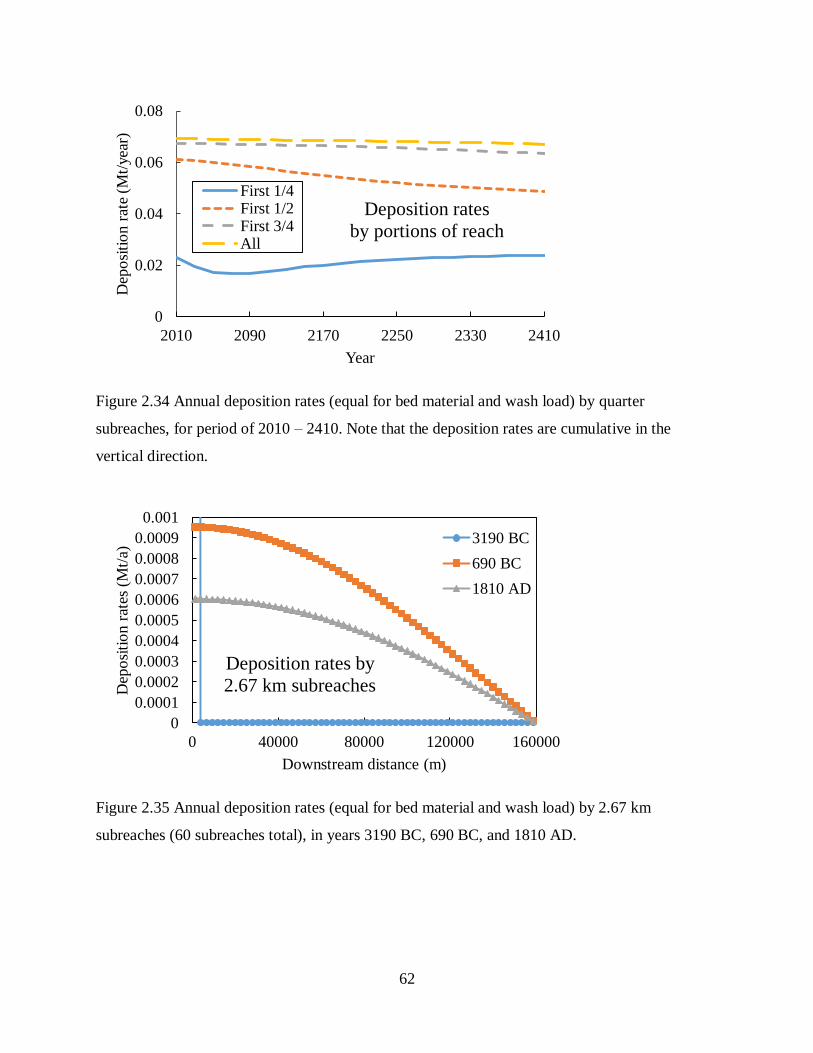
62

Figure 2.34 Annual deposition rates (equal for bed material and wash load) by quarter

subreaches, for period of 2010 – 2410. Note that the deposition rates are cumulative in the

vertical direction.

Figure 2.35 Annual deposition rates (equal for bed material and wash load) by 2.67 km

subreaches (60 subreaches total), in years 3190 BC, 690 BC, and 1810 AD.

0

0.02

0.04

0.06

0.08

2010 2090 2170 2250 2330 2410

Dep

osi

tio

n r

ate

(Mt/

yea

r)

Year

Deposition rates

by portions of reach

First 1/4First 1/2First 3/4All

0

0.0001

0.0002

0.0003

0.0004

0.0005

0.0006

0.0007

0.0008

0.0009

0.001

0 40000 80000 120000 160000

Dep

osi

tio

n r

ates

(M

t/a)

Downstream distance (m)

Deposition rates by

2.67 km subreaches

3190 BC

690 BC

1810 AD

63

Figure 2.36 Annual deposition rates (equal for bed material and wash load) by 2.67 km

subreaches (60 subreaches total), in years 1810, 1910, and 2010.

Figure 2.37 Annual deposition rates (equal for bed material and wash load) by 2.67 km

subreaches (60 subreaches total), in years 2010, 2210, and 2410.

0

0.005

0.01

0.015

0 40000 80000 120000 160000

Dep

osi

tio

n r

ates

(M

t/a)

Downstream distance (m)

Deposition rates

by 2.67 km subreaches

1810

1910

2010

0

0.004

0.008

0.012

0 40000 80000 120000 160000

Dep

osi

tio

n r

ates

(M

t/a)

Downstream distance (m)

Deposition rates

by 2.67 km subreaches2010

2210

2410

64

REFERENCES

Belmont, P., Gran, K. B., Schottler, S. P., Wilcock, P. R., Day, S. S., Jennings, C., Lauer, J. W.,

Viparelli, E., Willenbring, J. K., Engstrom, D. R., and Parker, G. (2011). “Large shift in

source of Fine Sediment in the Upper Mississippi River.” Environmental Science and

Technology 45:8804-8810

Brownlie, W. R. (1981). Prediction of flow depth and sediment discharge in open channels

Report No. KH-R-43A, W. M. Keck Laboratory of Hydraulics and Water Resources,

California Institute of Technology, Pasadena, California, USA;

http://caltechkhr.library.caltech.edu/7/01/KH-R-43A.pdf.

Dade, W. B., Friend, P. F. (1998). Grain-size, sediment-transport regime, and channel slope in

alluvial rivers. Journal of Geology 106, 661-675.

Dietrich, W. E. (1982). Settling velocity of natural particles. Water Resources Research 18(6),

1615-1626.

Eke, E. C. (2013). PhD Thesis, University of Illinois Urbana-Champaign, USA.

Engelund, F., Hansen, E. (1967). A Monograph on Sediment Transport in Alluvial Streams

Technisk Vorlag, Copenhagen, Denmark.

Engstrom, D. R., Almendinger, J. E., and Wolin, J. A. (2009). “Historical changes in sediment

and phosphorous loading to the upper Mississippi River: mass-balance reconstructions from

the sediments of Lake Pepin.” J. Paleolimnol, 41:563-588.

Ferguson R. (2010). Time to abandon the Manning equation? Earth Surface Processes and

Landforms 35, 1873-1876.

Hey, R.D., Thorne, C. R. (1986). Stable channels with mobile gravel beds. Journal of Hydraulic

Engineering 112(6), 671-689.

IPCC (2013). Climate Change 2013: The Physical Science Basis. Report, U.N.

Intergovernmental Panel on Climate Change, available at:

http://www.climatechange2013.org/.

Johannesson, H., Parker, G., García, M., Okabe, K. (1988). “Diagnostic study of the siltation

problem at the Wilmarth Power Plant cooling water intake on the Minnesota River.”

Project Report No. 77, University of Minnesota St. Anthony Falls Hydraulic Laboratory

Project Report No. 277.

65

Kelley, D. W., Brachfeld, S. A., Nater, E. A., and Wright Jr., H. E. (2006). “Sources of sediment

in Lake Pepin on the Upper Mississippi River in response to Holocene climatic changes.” J.

Paleolimnol, 35, 193–206.

Kim, W., Mohrig, D., Twilley, R., Paola, C., Parker, G. (2009). Is It feasible to build new land in

the Mississippi River delta? EOS 90(42), 373-374.

Lamb, M. P., Dietrich, W. E., Venditti, J. G. (2008). Is the critical Shields stress for incipient

sediment motion dependent on channel-bed slope? Journal of Geophysical Research

113(F02008).

Latrubesse, E. M. (personal communication). Data base for large tropical rivers:

latrubesse@austin.utexas.edu.

Lauer, J. W. and Parker, G. (2008). Net local removal of floodplain sediment by river meander

migration. Geomorphology 96(1-2), 123-149.

Lauer, J. W., Parker, G., Dietrich, W. E. (2008). Response of the Strickland and Fly River

confluence to postglacial sea level rise. Journal of Geophysical Research 113(F01S06).

Leopold, L. B., Maddock, Jr., T. (1953). The hydraulic geometry of stream channels and some

physiographic implications. Professional Paper 252, U.S. Geological Survey, Washington,

DC.

Li, C., Czapiga, M., Eke, E. C., Viparelli, E., and Parker, G. (accepted, May, 2014). “Variable

Shields number model for river bankfull geometry: bankfull shear velocity is viscosity-

dependent but grain size-independent.” J. Hydraulic Research.

MacDonald, T. E., Parker, G., Leuthe, D. P. (1991). “Inventory and analysis of stream meander

problems in Minnesota.” Report, St. Anthony Falls Laboratory. University of Minnesota.

Mueller, E. R and Pitlick, J. (2005). Morphologically based model of bed load transport capacity

in a headwater stream. Journal Of Geophysical Research, 110, doi:10.1029/2003JF000117,

14 p.

Musser, K., Kudelka, S., and Moore, R. (2009). Minnesota River Basin Trends, Mankato State

University, Mankato, MN USA. Pp. 64.

Nittrouer, J. A., Mohrig, D., Allison M. A. (2011). Punctuated sand transport in the lowermost

Mississippi River. Journal of Geophysical Research 116, 1914-1934, doi:

10.1029/2011JF002026.

66

Paola, C., Heller, P. L., Angevine, C. L. (1992). The large-scale dynamics of grain-size variation

in alluvial basins, 1: Theory. Basin Research 4, 73-90.

Parker, G. (1978). Self-formed straight rivers with equilibrium banks and mobile bed. Park 2.

The gravel river. Journal of Fluid Mechanics 89, 127-146.

Parker, G., Paola, C., Whipple, K. X., Mohrig, D. (1998a). Alluvial fans formed by channelized

fluvial and sheet flow. I: Theory. Journal of Hydraulic Engineering 124(10), 985-995.

Parker, G., Paola, C., Whipple, K. X., Mohrig, D., Toro-Escobar, C. M., Halverson, M.,

Skoglund, T. W. (1998b). Alluvial fans formed by channelized fluvial and sheet flow. II:

Applications. Journal of Hydraulic Engineering 124(10), 996-1004.

Parker, G. (2004). 1D Sediment Transport Morphodynamics with applications To Rivers and

Turbidity Currents (E-book; http://vtchl.uiuc.edu/people/parkerg/).

Parker, G. , Wilcock, P., Paola, C., Dietrich, W. E., Pitlick, J. (2007). Quasi-universal relations

for bankfull hydraulic geometry of single-thread gravel-bed rivers. Journal of Geophysical

Research Earth Surface, 112(F4), 21 p.

Parker, G., Muto, T., Akamatsu, Y., Dietrich, W. E., Lauer, J. W. (2008). Unraveling the

conundrum of river response to rising sea level: from laboratory to field. Part II. The Fly-

Strickland River System, Papua New Guinea. Sedimentology, 55(6), 1657-1688.

Parker, G. (2008) in Sedimentation Engineering processes: Measurements, modeling and

practice, Garcia, M. H., Ed. (ASCE, Reston, VA.) chap. 3, 165-251.

Parker, G., Shimizu, Y., Wilkerson, G. V., Eke, E., Abad, J. D., Lauer, J. W., Paola, C.,

Dietrich, W. E., Voller, V. R. (2011). A new framework for modeling the migration of

meandering rivers. Earth Surface Processes and Landforms 36, 70–86.

Recking A. (2009). Theoretical development on the effects of changing flow hydraulics on

incipient bedload motion. Water Resources Research 45, W04401:

16.doi:10.1029/2008WR006826.

Rijn, L. C. (1984). Sediment transport, Part II: Suspended load transport. Journal of Hydraulic

Engineering 110(11), 1613-1641.

Soar, P. J., Thorne, C. R. (2001). Channel restoration design for meandering rivers. Report,

ERDC/CHL CR-01-1, 416, Coastal Hydraulics Laboratory, U.S. Army Corps of Engineers,

Engineer Research and Development Center.

67

US Environmental Protection Agency. “National Summary of Impaired Waters and TMDL

Information.” Water Assessment and TMDL Information,

< http://iaspub.epa.gov/waters10/attains_nation_cy.control?p_report_type=T> (May 3,

2014)

Wilcock, P. (2009). “Identifying sediment sources in the Minnesota River Basin,” River

Sediment Colloquium,

<http://cnr.usu.edu/files/uploads/faculty/Belmont/wilcock_et_al_SedSynth_FinalDraft.pdf

> (May 3, 2014)

Wilkerson, G. V., Parker, G. (2011). Physical basis for quasi-universal relationships describing

bankfull hydraulic geometry of sand-bed rivers. Journal of Hydraulic Engineering 7(1),

739-753.

Wright, S., Parker, G. (2005). Modeling downstream fining in sand-bed rivers. I: Formulation.

Journal of Hydraulic Research 43(6), 612-619.

Wright, S., Parker, G. (2005). Modeling downstream fining in sand-bed rivers. II: Application.

Journal of Hydraulic Research, 43(6), 620-630.