Modeling the Tradeoff between Inventory and Capacity to OptimizeReturn on Assets in Production Scheduling

By

Cindy (Hsin-ying) WuMBA in Technology and Innovation Management, National Chengchi University, 2006

B.Sc. Electrical Engineering, National Chiao Tung University, 2003

and

Jos6 Antonio Gonzilez Duhart Mufioz de CoteB.Sc. Industrial Engineering, Universidad Panamericana, 2007

Submitted to the Engineering Systems Division in Partial Fulfillment of theRequirements for the Degree of

Master of Engineering in Logistics

at the

Massachusetts Institute of Technology

June 2013

C 2013 Cindy (Hsin-ying) Wu and Jos6 Antonio Gonzilez Duhart Mufloz de CoteAll rights reserved.

The authors hereby grant to MIT permission to reproduce and distribute publicly paper and electroniccopies of this document in whole or in part.

Signature of Author ................................................ ....Master of Engineering in Supply Chain Management ProgranA Enginee g Systems Division

May 10, 2013

S ignature of A uthor. .................................................. .... .......................................Master of Engineering in Supply in Mana tProgram, Engineering Systems Division

- 77May 10, 2013

Certified by...Dr. Bruce C. Arntzen

Executive Director, Supply Chain Master's ProgramMIT Center for Transportation and Logistics

Thesis Supervisor

Accepted by.... .......................................................Prof. Yossi Sheffi

Elisha Gray II Professor of Engineering Systems, MITDirector, MIT Center for Transportation and Logistics

Professor, Civil and Environmental Engineering, MIT

I

S~4 A(-TINC

. C

Modeling the Tradeoff between Inventory and Capacity to Optimize Return on Assets in

Production Scheduling

by

Cindy (Hsin-ying) Wu and Jose Antonio Gonzalez Duhart Munoz de Cote

Submitted to the Engineering Systems Division on May 10, 2013 in Partial

Fulfillment of the Requirements for the Degree of Master of Engineering in

Logistics and Supply Chain Management

Abstract

In the agrochemical industry, companies are challenged with an extreme seasonality in

demand driven by the crops' growing cycles. Therefore, balancing supply with such

fluctuating demand has been a struggle for most companies due to their capacity constraints.

One way to accommodate the demand is to stock enough inventory ahead of the peak

seasons, while the other is to increase the production capacity so that the companies can

react to the changing demand more quickly. However, either alternative comes at a

significant cost.

This paper examines the optimal mix of production capacity and inventory for a company to

meet customers' demand at the highest net present value (NPV) of operating assets value

add (OAVA). We use a multi-period, multi-stage, multi-product mixed integer linear

optimization model to determine the best combination of resources. Viable resource options

include stocking inventory ahead of the peak seasons, enhancing output through overtime,outsourcing production activities to a third party, and acquiring new assets for a particular

production stage. The results show that the optimal OAVA comes from a combination of all

these viable resources.

Additionally, the master production schedule, the resulting inventory levels, and the

recommended timings for external resources and asset acquisition are important takeaways

from our model. They serve not only as the guidance of the company's day-to-day

operations, but also as the quantitative analysis necessary to communicate with

stakeholders across different functional teams with potentially conflicting interests.

Thesis Supervisor: Dr. Bruce Arntzen

Title: Executive Director, Supply Chain Masters Program

2

"I have friends in overalls whose friendship

I would not swap for the favor of kings."

Thomas Alva Edison

Acknowledgements

We thank the following people without whom our research wouldn't have been possible:

Chris Nix, for answering every crazy question from us and challenging our different

approaches towards tackling this problem.

Dr. Bruce Arntzen, who had patience with us beyond what's humanly possible and

unparalleled eagerness to help us get hands on into the problem.

[INDO Systems, who provided us a temporal student license with unlimited number of

decision variables and constraints for their Obercool optimization software, What'sBest!,

which we used more than we care to remember.

Dr. Jonathan Byrnes, for fueling our initiative of writing this thesis in an exhilarating style.

Thea Singer, who forever pestered us into handing in the next section of our thesis, so

that we could get timely and vital feedback.

Our sponsoring company and the people behind it, including Joshua Merril, Carol Oliveira,

Bill Sowle, Andre Freitas, Brian Stockholm, Sarah Crete, Prashanth Krishnamurthy, Lisa

Foreman, Dave Winstone and Joe Krkoska, for setting up the way during the early stages

of the project.

3

<Cindy> On a personal note, I would like to thank the SCM family, Class of 2013, for making

this 10-month program an informative and enjoyable learning journey. Every challenge I

faced with made me a more humble learner, and every encouragement from the SCM family

empowered me to explore further, either in research or beyond. Lastly, I'd like to thank Jose,

my thesis partner and amigo para siempre, for taming my willfulness with endless tolerance,

making me see what I couldn't, and inspiring me to live to my true self.

<Jose> Several people helped me throughout the process of culminating this dream and

journey, for whom I feel the deepest gratitude...

Mom, for everything I am or ever will be, I owe it to you.

Horace and Gabs, you've been a living example and inspiration.

Dad, the first and best engineer I've ever known.

CONACYT, FUNED and FIDERH, institutions of the best country in the world, who were theofficial sponsors of this quest.

Queko, Trigo, Alvaro and Villarro, for being the best friends I could've ever asked for.

Maps, my partner in life, for kindling my spirit day and night, everyday this whole time.

Diego Castaneda, Ivan Rosenberg and Miguel Angel Ramirez, for the extreme trust you'veplaced on me.

Francisco Ortiz, Margarita Hurtado, Vicky Carreras, Jorge Tellez, Juan Carlos Padilla, Juli nFernandez and Andres de Antonio Crespo, for your teachings, recommendation letters,and words of wisdom.

SCM Class of 2013, for seldom do I have the pleasure of sharing the room with such abunch of peculiar, yet remarkable and outstanding people.

f , for every lesson learned, for your trust, for your help and your invaluablefriendship. It has truly been an honor having you as my thesis partner.

4

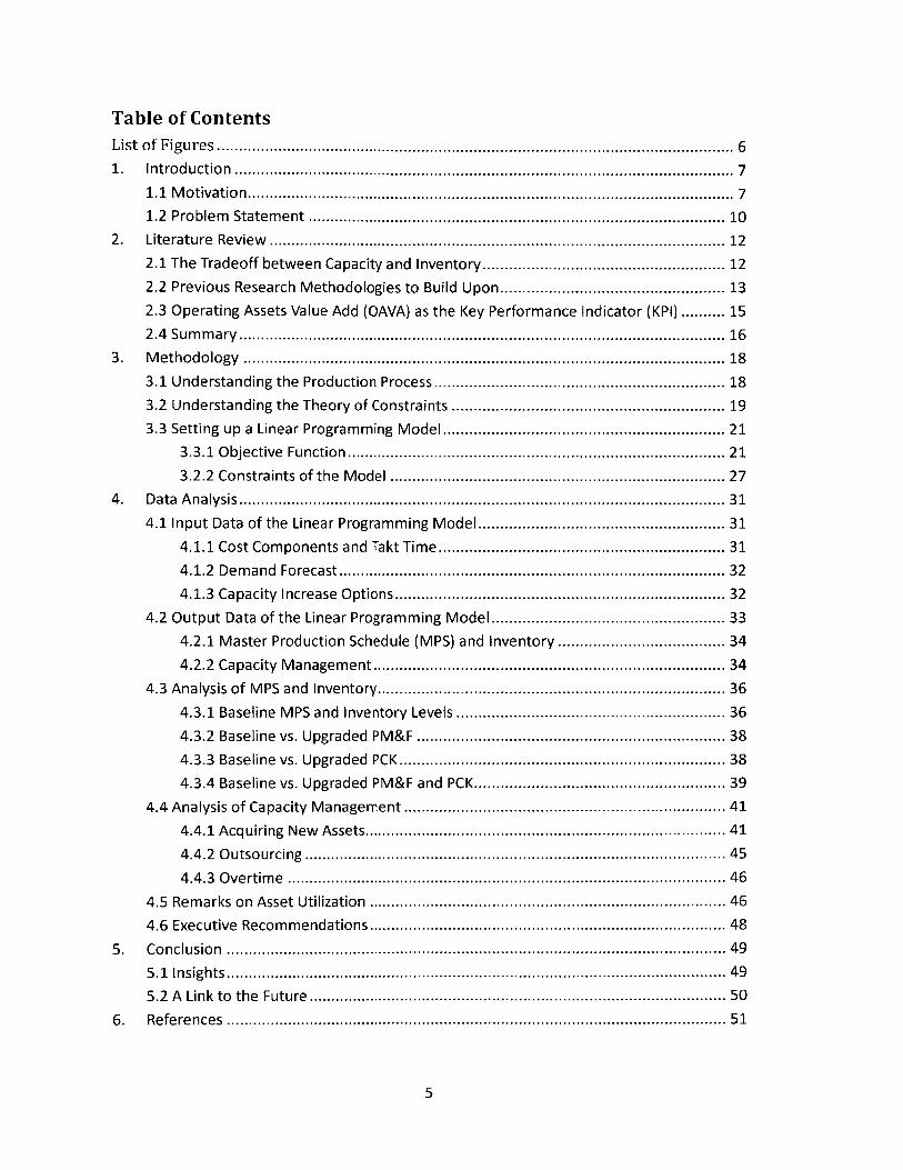
Table of Contents

List of Figures ...................................................................................................................... 6

1. Introduction .................................................................................................................. 7

1.1 M otivation............................................................................................................... 7

1.2 Problem Statem ent ............................................................................................ 10

2. Literature Review ........................................................................................................ 12

2.1 The Tradeoff between Capacity and Inventory.................................................... 12

2.2 Previous Research M ethodologies to Build Upon................................................ 13

2.3 Operating Assets Value Add (OAVA) as the Key Performance Indicator (KPI) ..... 15

2.4 Sum m ary ............................................................................................................... 16

3. M ethodology .............................................................................................................. 18

3.1 Understanding the Production Process ............................................................... 18

3.2 Understanding the Theory of Constraints .......................................................... 19

3.3 Setting up a Linear Program m ing M odel............................................................. 21

3.3.1 Objective Function .................................................................................. 21

3.2.2 Constraints of the M odel ......................................................................... 27

4. Data Analysis............................................................................................................... 31

4.1 Input Data of the Linear Program m ing M odel.................................................... 31

4.1.1 Cost Com ponents and Takt Tim e............................................................. 31

4.1.2 Dem and Forecast .................................................................................... 32

4.1.3 Capacity Increase Options....................................................................... 32

4.2 Output Data of the Linear Program m ing M odel.................................................. 33

4.2.1 M aster Production Schedule (M PS) and Inventory ................................... 34

4.2.2 Capacity M anagem ent .............................................................................. 34

4.3 Analysis of M PS and Inventory............................................................................ 36

4.3.1 Baseline M PS and Inventory Levels .......................................................... 36

4.3.2 Baseline vs. Upgraded PM &F ................................................................... 38

4.3.3 Baseline vs. Upgraded PCK....................................................................... 38

4.3.4 Baseline vs. Upgraded PM &F and PCK....................................................... 39

4.4 Analysis of Capacity M anagement ..................................................................... 41

4.4.1 Acquiring New Assets.............................................................................. 41

4.4.2 Outsourcing ............................................................................................ 45

4.4.3 Overtim e ................................................................................................ 46

4.5 Rem arks on Asset Utilization ............................................................................. 46

4.6 Executive Recom m endations .............................................................................. 48

5. Conclusion .................................................................................................................. 49

5.1 Insights.................................................................................................................. 49

5.2 A Link to the Future ............................................................................................. 50

6. References .................................................................................................................. 51

5

List of Figures

Figure 3-1. Conceptual Model of the Production Process ................................................ 19

Figure 3-2. The Illustration of Constraint Identification Process........................................ 20

Figure 3-3. Proxy Value given no capacity increases ........................................................ 26

Figure 3-4. Proxy Value when there is a capacity increase ................................................ 26

Figure 4-1. Cost Components and Takt time of both products ......................................... 32

Figure 4-2. Excerpted Table for the 10-year Demand Forecast.......................................... 32

Figure 4-3. Assets Value and Capacity Limits for Acquired Assets ..................................... 33

Figure 4-4. Capacity Lim its for Overtim e ......................................................................... 33

Figure 4-5. Excerpted Table for MPS and Inventory .......................................................... 34

Figure 4-6. Excerpted Table for Acquiring New Assets ...................................................... 35

Figure 4-7. Production Process......................................................................................... 36

Figure 4-8. Production and Inventory Levels for Baseline Capacity ................................... 37

Figure 4-9. Production and Inventory Levels with Upgraded PM&F Capacity.................... 38

Figure 4-10. Production and Inventory Levels with Upgraded PCK Capacity...................... 39

Figure 4-11. Production and Inventory Levels with Upgraded PM&F and PCK Capacity ....... 40

Figure 4-12. PM &F Capacity Upgrade in Year 5................................................................. 42

Figure 4-13. PM &F Capacity Upgrade in Year 8................................................................. 42

Figure 4-14. PCK Capacity Upgrade in Year 8 ................................................................... 44

Figure 4-15. PCK Capacity Upgrade in Year 10 ................................................................. 44

Figure 4-16. PIM&F Capacity and Production Management in Year 7 ................................ 45

Figure 4-17. Optimal Scenario vs. Maximum Utilization .................................................. 47

6

"Out of clutter, find simplicity. From discord, find harmony.

In the middle of difficulty lies opportunity."

Albert Einstein

1. Introduction

1.1 Motivation

* * * * * * * * * * * * * * * * * * * *

In the fall of 2012, Alan A', the Global Supply Chain manager of a division in a large agrochemical

company, was assessing how his division could increase output after receiving a financial report by

the company's management review committee. The report indicated significant lost sales during the

past two quarters, damaging the company's profitability, and Alan's group was directly responsible

for them.

Alan had seen this coming six months earlier. The moment when the production manager reported

that production couldn't catch up to demand due to a recent upside, the sales team could not stop

yelling: "No farmer will wait on us before starting their growing season! They love our products but

are now buying from others. That's easy money going into competitors' pockets. Easy money!"

Unfortunately, in-house capacity had already reached near-full utilization, and the request for extra

capacity would take 2~3 years for the long-winded process of evaluation, approval paperwork and

final follow-through. Outsourced resources were 40% more expensive than in-house resources but

were already engaged given such an extenuating situation. Despite this, there was still a long way to

go before being able to fulfill the upsized demand. Pre-built inventory wasn't available, as the factory

had purposely kept it low to minimize inventory holding costs, even though they did not have upside

manufacturing capacity.

The names and characters in the story of this section are fictitious.

7

As Alan was pondering actions that would have prevented the losses, his desk phone rang. "The sales

forecast for next year is looking at a potential 20% increase, with another 20% for the year after.

Whatever went wrong this year, FIX IT, before it gets bigger!" the sales manager thundered.

Alan looked at the clock. It was about time to talk with the MIT research team about how to address

the challenge, one that had significant financial impact, but involved stakeholders from

cross-functional areas with conflicting interests. He wondered how these young professionals from

MIT would approach such a headache and help turn the situation around.

* * * * * * * * * * * * * * * * * * * *

In a large but almost empty study room on the MIT campus, Cindy Wu was shutting down her

computer, ready to rest her dry and tired eyes after staring at the screen all night. She looked up at

the clock and found the arms already pointing to 2am. Jose Duhart, raising his head from stacks of

papers after scrutinizing them for hours, stretched his neck and made a final comment, "Tomorrow is

going to be our big day. We'll be solving a puzzle that's worth millions of dollars." "Agreed. And I feel

rich already," joked Cindy as usual.

Cindy Wu and Jose Duhart were the two MIT SCM students who signed up for this project due to the

challenging business nature of the agrochemical industry, where the demand pattern was highly

seasonal and thus more difficult to plan and fulfill. Their advisor, Dr. Bruce Arntzen, had cautioned

them about the complexity of this project as it required heavy quantitative and analytical skills, as

well as software modeling and debugging techniques.

"Even better," both students commented excitedly. Indeed, nothing motivated them more than

intense intellectual exercises. Most importantly, knowing that the insights they would acquire

through this research could be applied to industries and businesses with similar challenges

empowered them to work even harder.

8

After an entire night's hard work, the whiteboard captured the priorities for the next steps.

1. Define the problem and challenges faced by managers.

2. Define the key questions that our project strives to answer.

3. Review relevant literature to understand the tradeoff between capacity and inventory; find

out potential research methodologies and performance indicators.

4. Understand the production process and the theory of constraints, and set up a linear

programming model.

5. Validate the linear programming model and analyze the output.

6. Provide recommendations to assist with managerial decision making.

As they walked back to their dorms, conversations were still on-going.

"Pre-building inventory eliminates the need for capacity investment, and vice versa. Between the

two extremes, there must be a middle ground that presents the best tradeoff." "..., which is one of

the key objectives of this project. And the real challenge would be finding consensus between

managers with conflicting goals." "True. It's gonna be a solution that requires joint improvement

effort across all functional teams." "... also a guideline for all of these teams to know which product

to produce, for how much volume and at what time."

From this point forward, the youthful duo ventured on an intellectual challenge that would test their

skills as analysts, modelers, problem solvers and effective communicators.

9

1.2 Problem Statement

Our sponsoring company is an agrochemical company offering herbicides, pesticides and

seed technologies that minimize the level of undesirable weeds, insects and diseases. Due

to the seasonal fluctuation of demand in the agricultural industry, fulfilling customers'

demand is a challenge that, if not handled well, might lead to significant loss of sales. In fact,

the company has suffered from revenue losses for this reason in the past years. As the

agrochemical market keeps growing, allocating resources to fulfill customers' demand is one

of the company's top priorities.

One way to accommodate the fluctuating demand is to stock enough inventory ahead of the

peak seasons. The other extreme is to increase the production capacity so that the company

can react to the changing market demand more quickly. Traditional management practice

prescribed that businesses should maximize asset utilization in order to reduce costs.

Therefore, many plant managers would starve the plant of new equipment and rely on

pre-building inventory to meet seasonal demand. This approach yielded excellent

equipment utilization at the expense of overall financial performance. Literature shows that

relying solely on pre-built inventory to meet variable demand is not optimal. Hence, the

question that this project seeks to answer is: What is the optimal mix of production capacity

and inventory for the company to meet customers' demand at the highest net present value

(NPV) operating assets value add (OAVA) over the planning horizon?

The project, given the limited time frame, will focus on a single weed killer product,

codename Mustang, because its current production capacity cannot fulfill its total demand

for the peak months. This project will use a multi-period mixed linear programming model

10

to find an optimal solution for the company's production planning. The solution will include

the inventory level per period, the utilization rate for each of the resources involved in the

manufacturing of Mustang, the total costs of implementing this solution, and the NPV for

OAVA. To this end, we will explore the information available on several aspects of the

current production processes, including the current capacities of each line producing

Mustang, the demand of Mustang in the past, and the manufacturing cost per unit.

This project aims to improve the company's financial performance and customer service

level by both fulfilling demands in peak seasons while achieving the highest level of return

on operating assets in the form of OAVA. The research results, including the optimization

model, research methodologies and implications, can be leveraged by different product

lines within the same industry or even different industries with similar problems.

11

"If I've seen further than others, it is by standing on shoulders of giants."

Isaac Newton

2. Literature Review

This literature review is presented in four sections. We start by discussing the tradeoff

between capacity and inventory management, as well as the devious concept of achieving

higher financial return with a lower capacity utilization rate. In the second section we cover

the research methodologies available to optimize the mix between capacity and inventory

across different industries, product characteristics and business needs. Subsequently, we

present the performance indicators that determine the effectiveness of applying certain

tradeoff scenarios according to different business strategies. In the final section, we

summarize the methodologies and performance indicators that we adopt in this research

based on our sponsor company's business needs and challenges.

2.1 The Tradeoff between Capacity and Inventory

Common management practice suggests that businesses should maximize asset utilization to

reduce costs. As Hayes and Wheelwright (1984) commented, "Unused capacity generally is

expensive." As a result, managers normally favor excess inventory over excess capacity in

response to seasonality and fluctuation in demand.

However, Krajewski et al. (1987) and Monden (1981) found that under a Just-In-Time

strategy, production lines need to keep extra capacity by 10% to 18% to buffer the need for

extra inventory and maintain the equipment lifetime. Goldratt and Cox (1992) further

challenged the assumption that capacity utilization is directly correlated with the net benefit

to a manufacturing company. They stated that capacity utilization in non-restriction assets is

12

irrelevant, while at bottlenecks it should be as high as possible.

Colgan (1995) took an extra step by studying the capacity utilization and inventory policies in

a personal computer production line, building optimization models to simulate alternative

scenarios, and comparing the financial results from these scenarios. He concluded that

maximized utilization rates do not necessarily drive the best financial results.

Bradley and Glynn (2002) derived the same conclusion with a different approach. They

developed a mathematical expression to assist in deciding the joint optimization of

inventory and capacity based on "minimum cost operation" and found that high capacity

utilization might not always suit the cost-down purpose as capacity may not always be

expensive. Their numerical model further showed that the total cost could increase

significantly if the capacity level was overly restricted.

Based on these research findings, we understand that both capacity and inventory are

indispensable factors that need to be balanced and jointly considered in seeking an

optimized financial benefit for an organization. As Goldratt and Cox (1992) explained,

keeping extra inventory or extra capacity beyond a certain limit should be deemed

unproductive and, therefore, eliminated because it is an effort that either leaves the net

profit unaffected or decreases it. Consequently, finding the right mix between these two

factors is one of the key objectives of this research project.

2.2 Previous Research Methodologies to Build Upon

Goldratt and Cox (1992) developed the theory of constraints in a manufacturing process and

introduced the concept of finding next constraints continuously after the existing one is

13

resolved. The measures in controlling the flow of production process are the metrics in

identifying constraints. We will use Goldratt and Cox's approach for this project; by

reviewing the production process on an ongoing basis and incrementing capacity at the

constraints, we will be able to increase capacity as a whole and identify new constraints in

the system.

Building on the theory of constraints, Colgan (1995) identified several tradeoff scenarios,

called "line configurations" in his research, by finding constraints one after another on a

personal computer production line. He further built a multi-period and multi-station

mathematical model for a single product line. The model simulated the financial

performance of these scenarios based on the optimized return on operating assets (ROOA),

a strategy that we will elaborate upon in the next section. Colgan's work serves our research

as a baseline from which we can leverage the mathematical construction of the model. Our

scope will expand on Colgan's formulation because it involves more than one product line,

thus adding a multi-product complexity.

Bradley and Glynn (2002) took a different approach towards finding a joint optimization of

capacity and inventory. They derived a mathematical expression based on the minimum cost

operation for a single-product, single-station, make-to-stock manufacturing process. As with

Colgan's, Bradley and Glynn's work serves as a baseline in understanding the mathematical

modeling. Building on their work, this research will go beyond a single product, station and

time period.

Jammernegg and Reiner (2007) studied the change of business processes from

make-to-order to assemble-to-order in the telecommunication and automotive industries,

14

and simulated the optimal solutions of different tradeoff scenarios based on both costs and

service level objectives. As with Colgan's and Bradley & Glynn's, this optimization model is

limited to a single period and single product.

Mincsovics et al. (2009) introduced in their model the concept of contingent capacity, which

refers to the additional capacity that can be acquired with a given lead time and can be

disposed of after it is no longer required. Additionally, they dealt with a product which can

be backlogged and associated a cost for backorders, aiming to determine the optimal

permanent capacity of a system and acquire contingent capacity accordingly. They stated

that the relative value of contingent capacity is inversely proportional to the lead time it

takes to be available. At the same time, contingent capacity's value is directly proportional to

the cost of backordering. In the production process that we studied during the development

of this thesis project, adding capacity requires a significant dollar investment and cannot be

disposed of. Hence, once we add extra capacity it is permanent. We can leverage from

Mincsovics's work by assuming an infinite time to dispose of installed equipment.

2.3 Operating Assets Value Add (OAVA) as the Key Performance Indicator (KPI)

Goldratt and Cox (1992) introduced relevant key performance indicators (KPI), such as

throughput, inventory, and operational expense, as well as a way to measure and manage

these indicators. These authors provide a baseline approach to find a constraint in a

production process, increment its capacity, which then increases the net throughput of the

system, and loop back to finding new constraints in the system. These steps are part of the

methodology this thesis project relies on. In the mathematical expression developed by

Bradley and Glynn (2002), the minimum average operating cost was the main metric in the

15

objective function that drives the optimal capacity and inventory policies. Jammernegg and

Reiner (2007) included fl-service level (fill rate), delivery performance and work-in-process

pallets as performance improvement measures.

The concept of return on assets (ROA) has been used across several industries by decision

makers (Anthony and Dearden 1980, Kaplan and Atkinson 1989), despite its weaknesses

such as its short-term representation of the company's financial performance instead of an

overall evaluation throughout the lifetime of the equipment. The ROA serves as an

introduction to one of the main metrics that we will be using in this thesis project, which is

the Return on Operating Assets (ROOA).

Colgan (1995) and Bradley and Arntzen (1999) adopted the derivative form of ROA and

termed it the Return on Operating Assets, which bypassed some corporate level financial

details irrelevant to the research scope and focused on the company's financial gain resulted

directly from the invested assets. 3M's ROOA Capacity Planning Project Team (1994)

introduced a modified linearized ROOA metric, termed operating assets value add (OAVA), to

reflect the financial gain. OAVA is a linear expression and can thus be optimized using

mixed-integer linear programming, as opposed to ROOA, which is a ratio and thus non-linear.

These metrics will serve as a basis to decide the best line configuration and at the same time

the best asset utilization for the entire production process.

2.4 Summary

From the literature review above, we understand that to help the company fulfill its highly

seasonal and fluctuating demand, a joint optimization strategy of both capacity and

inventory policies is essential. Furthermore, a multi-product, multi-station and multi-period

16

model is necessary to capture the complexity and challenges of the company's business

practices. Finally, we will adopt a modified ROOA metric, the OAVA, to directly reflect the

financial gain introduced by a particular capacity investment.

17

"We shape our buildings;

thereafter, our buildings shape us."

Winston Churchill

3. Methodology

Our methodology is comprised of three sections. We start by introducing the company's

existing production process to understand its business need and potential areas for

optimization. Subsequently, we build a linear programming optimization model that

supports multi-period, multi-product and multi-station characteristics. Following the theory

of constraints, the model will identify limitations in the company's production process and

the optimal line configuration as a potential solution to address these constraints. The

output of the simulation will include the master production plan and the combination of all

viable resource options.

Since it takes 2 to 3 years to implement a decision to add line capacity, we are modeling for a

10-year horizon. While the demand each year displays a similar pattern of seasonality with

the peak in Sept., Oct. and Nov., the overall demand profile moves higher each year as sales

increase. The model is looking out 10 years in advance trying to determine the optimal

operating strategy in each month of this horizon and when to add capacity.

3.1 Understanding the Production Process

The company's production process consists of four main stages: pre-mix, formulation,

storage and packaging, as illustrated in Figure 3-1. In the pre-mix stage, active ingredients

are added into a heated tank for preliminary mix before flowing into the formulation stage,

where more ingredients are added and mixed for a longer period of time. After formulation,

the chemical product is stored in the tanks in the storage stage and will be packaged into

18

different sizes of containers according to the demand in the packaging stage.

Drums

Figure 3-1. Conceptual Model of the Production Process

3.2 Understanding the Theory of Constraints

From the four stages in the production process, also called "stations" in our research and

software model, our model will find out where the first constraint bottleneck is by

calculating the capacity in all stations. In our research, a constraint is defined as the station

in the production process where the capacity is lowest among all stations and, upon capacity

expansion, could increase the output in both the station and the whole process. Out of the

four stations in the production process, we are considering capacity expansion at three

stations: pre-mix & formulation, storage and packaging.

After identifying the first constraint and increasing the station's capacity to fix the first

constraint, the bottleneck will no longer be found in the same station. Our model repeats

the process to find the second constraint, the third, etc., as needed by the research. Figure

3-2 shows the conceptual constraint identification process.

19

1r Constraint

2 "d Constraint

3rd Constraint

Figure 3-2. The Illustration of Constraint Identification Process

The model will calculate the net present value of the OAVA for each time the constraint's

capacity is increased, to evaluate the financial return generated by the operating assets.

Starting from the baseline where no additional capacity is invested, the OAVA might go

either up or down after a capacity investment decision is made. As more capacity is added,

the OAVA values corresponding to each capacity alternative are captured and compared.

Additionally, other factors that can change the OAVA are working overtime, outsourcing and

pre-building inventory (either intermediate or finished goods). By working overtime we can

slightly expand the capacity of each stage incurring in the additional cost of the extra time

for labor and utilities. Outsourcing to a third-party manufacturer can offset or delay the

system's need to increase its capacity in one or multiple stages, but at the cost of paying a

high markup for the labor and utilities components. Finally, pre-building inventory can avoid

the need for investing in a capacity expansion, but instead will come at the cost of holding

such inventory for the total time it was held.

The model will evaluate OAVA using different combinations of acquiring extra capacity,

working overtime, outsourcing, and pre-building inventory. Each new combination will yield

a different OAVA. Every time the new value for OAVA is higher than the previous one, the

model will keep that line configuration. At some point, the value of OAVA will reach its peak,

and future investment, whether it is on capacity, overtime, inventory, or outsourcing, will no

longer push OAVA higher and might even cause it to decrease. That peak value is where the

20

model finds the optimal solution.

3.3 Setting up a Linear Programming Model

Now that we have understood the production process and the potential bottlenecks, we will

further develop a mathematical representation of the system that a computer can

understand and optimize. The software tool we will be using for this optimization is LINDO

Systems Inc.'s What'sBest!, a powerful add-in tool to Microsoft Excel's Solver. What'sBest!

has the advantage of dealing with multiple times the decision variables and constraints that

Excel Solver can handle.

3.3.1 Objective Function

We start by defining the objective function Z as the NPV of the OAVA at the annual

discount rate r over the planning horizon and aim to maximize it.

MAX: Z = NPV(r,OAVA)

= T (Revenuet - Costt) x (1 - Tax) - Cost of Capital x Asset Valuet

Z , = (1 +r)tt=o

Where:

T = number of time periods in the planning horizon; for our research 120 periods

r = Annual holding cost expressed as a percentage, for our research 12%

Breaking down each component of the objective function we obtain the following:

e Revenue

Revenue is estimated by first calculating the total cost of goods produced and then marking

that up by a factor.

21

Revenuet = Di,t x (R/ + LX + UMi X FrevVi VM

Where:

Di,t= Demand of product i at time t

Rmi = Cost of raw materials in machine M per unit of product i

LMi = Cost of labor in machine M per unit of product i

UMj = Cost of utilities in machine M per unit of product i

Frev = Factor for revenue markup

Since demand caps the amount of product that can be sold, revenue comes from the

demand multiplied by the associated manufacturing costs times a coefficient, defined by

the company, which in our research was set to 135%.

Cost

Cost = Holding Cost + Production Cost + Depreciation

The cost function has 3 main components that can be broken down to the following:

o Holding Cost

Holding Costt Invm,i,t +ln,1,t_1 m (Rm,i + Lmnv + Umi) x r

Where:

Invm,i,t = Inventory in machine M of product i at time t

As Silver et al. (1998) put it, holding cost includes the cost of opportunity of the investment,

the expenses of managing warehouses, handling and counting, special storage necessities,

deterioration, damage, shrinkage, and obsolescence among others. In this research, we first

22

average the ending inventory of two subsequent time periods, and then multiply it by the

cumulative manufacturing cost up to the current stage in the productive process as the

inventory value. Finally, we multiply the inventory value by the annual holding cost. Thus,

the cost of holding finished goods is always higher than holding work-in-process inventory.

For our research, we used an annual holding cost of 12%.

o Production Cost

Production Cost = Manufacturing + Outsourcing + Overtime

There are different ways in which the company can get the necessary products to satisfy

demand: either by manufacturing the products in-house or outsource to a third party at a

premium cost. In addition, the manufacturing process can be done in either the regular time

or the more expensive overtime option if required.

o Manufacturing Cost

Manufacturingt =pm,i,t x (RMj + LM,i + UM,i))

VM,i

Where:

PM,i,t = Produced units at machine M of product i at time t

Each stage in the production process has the need for raw materials, labor and utilities input,

all of which come with an associated cost. The manufacturing cost is calculated as the

product of the number of produced units multiplied by the sum of all cost components.

o Outsourcing Cost

Outsourcingt = (outit x (Ruj + (LM, + UM,i) x Fout)

Vi VM

23

Where:

Outit = Outsourced units of product i at time t

Fout = Factor for outsourced products

A third party supplier of finished goods can manufacture the product at a higher price than

producing it in-house. However, the cost for the raw materials remains exactly the same,

given that the company provides the external contractor all the required raw materials. The

labor and utilities costs increase by a markup of Fout which the company established at

40%. Similar to the manufacturing cost, we multiply the number of outsourced products by

the associated costs to calculate the outsourcing cost.

o Overtime (OT) Cost

Overtimet = (Overm,it X (RMI + (LM,i + UMI) X Fover))VM,i

Where:

Overi,t = Produced units during OT at machine M of product i at time t

Fover = Factor for production under overtime

As in the outsourcing cost, the cost for raw materials remains unchanged. Similarly, the costs

for labor and utilities are increased by a markup of Foyer which is set to 25%. Similar to the

manufacturing cost, we multiply the number of products manufactured during overtime by

the associated costs to calculate the overtime cost.

o Depreciation

Depreciation = Bm,,k X tk)

VM,k

Where:

VM,k = Value of a brand new machine M with capacity alternative k

24

Bmtk 0 if we choose not to invest for machine M at time t in alternative k1 if we choose to invest for machine M at time t in alternative k

Lm = Useful lifespan of machine M expressed in number of time periods

In our research, we use a straight-line depreciation approach to account for the cost of

machines. Once a new machine is added, the model adds a fixed amount depreciation

payment for all future periods. We multiply the binary variable times the fraction of the cost

for the corresponding machine. The company considers Lm to be 10 years, which is equal

to 120 time periods.

* Cost of Capital

Cost of Capital = is a constant value that the company determines at which it considers

the minimum annual return on capital investment should be. For our research, we were

provided a Cost of Capital of 12% but can be adjusted in the model to test different

scenarios and perform sensibility analysis.

e Average Asset Value

Average Asset Value = Proxy Capacity Value + Inventory Value

The operating assets that the company employs in the production process consist of two

main points; namely, capacity and inventory. On one hand, capacity encompasses everything

related to machinery and physical equipment such as containers, tank, packing lines, etc. On

the other hand, inventory refers to either work in progress (WIP) flowing through the system

or finished goods (FG).

o Proxy Capacity Value

Proxy Capacity Value = n x (BM,t,k x VM2k)t=1 VM,k

25

We decided to use an approximation for the capacity value since it significantly trims

complexity on calculations while illustrating the point of having to make an additional

investment at the same time. The proxy contrasts with the instantaneous value in that it

considers the average value of the asset, since this will be replaced after the end of its useful

life. Figure 3-3 depicts the conceptual pattern that the asset value will follow, given that no

capacity increase will be pursued over time.

C

C

tirne- Proxy Capacity value

- Instantaneous Capacity value

Figure 3-3. Proxy Value given no capacity increases

Similarly, the asset value increases when it undergoes an expansion in capacity. Figure 3-4

shows the conceptual behavior of the proxy value when capacity changes.

Lu

LA

EW)

- Proxy Capacity Value time

- instantaneous Capacity Value

Figure 3-4. Proxy Value when there is a capacity increase

26

The model first captures half of the value of the equipment at each time period. Then it

multiplies the half value by the binary variable as the proxy value. Finally, it takes the

average of these proxy values over the whole planning horizon.

o Inventory Value

Inventory Value = (v ,t [InvMit I n v,i,t_1 m 1(Rm,i + Lm,i + Um,i)

The other part of the assets corresponds to the inventory. The model captures the value of

all work in progress and finished goods in the production process and takes the average over

the planning horizon.

3.2.2 Constraints of the Model

The model will be subject to the following bounds:

* Meet Demand

For each product, a demand pattern broken down in each time period must be met.

InVN,i,t-1 + PN,i,t + OUti,t + OverN,i,t - InVN,i,t > Di,t Vi, t

Where:

N = Number of machines in the production process

Since machine N is the last stage in the production chain, it turns WIP into FG. Thus,

demand will be satisfied with the summation of last period's FG ending inventory and this

period's FG production, plus outsourced items and FG produced during overtime minus the

FG inventory left behind at the end of the period.

* Stage Dependence

27

Production in a given stage cannot exceed the production of the previous stage plus the

inter-stage inventory.

IVM-1,i,t-1 + PM-1,i,t - IfvM-1,i,t - PMjit VM, i, t

Capacity Limit

The machines cannot produce more than a certain limit, defined by the available work hours

and the time it takes to produce each product.

Y(PM~it M Tm): KM,t V M, i, t

Vi

Where:

TM,i = Time it takes for machine M to produce a unit of product i

KM,t = Capacity available in time units for machine M at time period t

For a multi-product model, production capacity cannot simply be defined in terms of volume

produced, since the consumption of resources for each product could be significantly

different. Instead, we define time available at each machine as capacity. The number of units

produced of each product times the amount of time required to produce each must be less

than or equal to the available capacity for that machine.

* Capacity Expansion

Alternatives for choosing extra capacity in each machine are mutually exclusive.

I BM,t,k = 1 VM, tVk

Furthermore, any capacity installed in the past must be present in the current time period.

In other words, the present capacity of any piece of equipment must be at least, as much as

the capacity in the previous period.

28

* Outsourcing

The third party vendor will only accept contracts that exceed certain amount of product. At

the same time, the external manufacturer is constrained by a fixed value.

YOutt i lt - Xt VtVi

Outti ! t ' Yt vtVi

Where:

flt = Binary variable to decide whether to pursue outsourcing at time period t

Xt = External manufacturer's minimum acceptable contract at time period t

Yt = External manufacturer's capacity limit at time period t

* Non-Negativity

Values for inventory, units produced and finished goods must be greater than or equal to

zero.

Invm,i,t 0

PM,i,t > 0

- Integer numbers

This constraint is optional. We can force the model to use only integer numbers for the

decision variables, in case it is not possible to produce fractions of units at a given stage or

for a particular product. In this research, we don't use this constraint so that the model

could be kept linear and the computing complexity is kept low.

PM,i,t 1E Z

Additionally, to see the expected value for any particular variable at any period of time t of

29

Bu,t_1,k 5 Bm tk vM, t, k

the model, we will have different state variables and decision variables:

* Number of production units in each stage

These will be the decision variables of the model. These numbers represent the quantity of

each product that each machine will produce at each time period.

* Amount of inventory at each stage

This results when the sum of the current production and the inventory from the previous

period exceeds the demand for the current time period and is recorded for each product at

each time period.

* Amount of consumed capacity for each machine at each time period

With the constraint and logic among all variables properly set up, our linear programming

model's algorithm will determine the production schedule and the capacity alternatives that

maximize our objective function, as well as display the costs and other state variables that

give us insight into a more cost-effective manufacturing process.

30

"All models are wrong, but some are useful."

George E.P. Box

4. Data Analysis

In this section, we will introduce the linear programming model constructed to find out the

mix of capacity and inventory that generates the most operating assets value add (OAVA).

Detailed instructions of how to use the model are also covered. The planning time horizon

within the scope of this research is 10 years with each month as an individual period.

4.1 Input Data of the Linear Programming Model

4.1.1 Cost Components and Takt Time

Figure 4-1 below summarizes the cost components that comprise the production costs and

inventory holding costs. For brevity, "Product" is shortened as "Prod", "Raw Material" as

"Raw" "Pre-Mix & Formulation" as "PM&G", "Packaging" as "PCK", "hour" as "hr", and

"kiloliter" as "kL". The production cost of each product consists of raw material, labor and

utility, with the units defined as dollar per kiloliter, whereas the inventory holding cost is a

function of both the production cost and the monthly holding cost coefficient. The "Takt

time" is defined as the time it takes (measured by hour) to produce one kiloliter of a product

and is used to calculate the consumed capacity in a certain stage.

The cells in yellow provide cost components and takt time for the stage "PM&F", while the

cells in green are for "PCK."

31

Monthly Holding 1.25% %

Raw (PM&F) 2,670 1,660 $/kL

Raw (PCK) 360 360 $/kL

Labor (PM&F) 620 - 600 $/kLLabor (PCK) 460 450 $/kL

Utilities (PM&F) 80 60 $/kL

Utilities (PCK) 40 30 $/kLTakt time (PM&F) 0.40 0.40 hr/kL

Takt time (PCK) 0.32 0.32 hr/kL

Figure 4-1. Cost Components and Takt time of both products

Such cost components, as well as other important cost information, including annual cost of

capital, overtime markup, outsourcing markup, tax and use of depreciation, can be filled in

by the user through the "Inputs" tab.

4.1.2 Demand Forecast

The demand forecast could be filled in by the user for each product through the "Forecast"

tab. The data will then be populated into the model in the same format as shown in Figure

4-2 below as another set of input needed to set up constraints.

* 1451 3031 4321 2761 1601 4031 2391 3391 9521 8011 1,1421 7431 305* 307 644 918 586 340 857 508 720 2,023 1,703 2,427 1,578 648

Figure 4-2. Excerpted Table for the 10-year Demand Forecast

4.1.3 Capacity Increase Options

As applicable to our sponsor company's operations, there are three options to increase

capacity: acquiring new assets, outsourcing and overtime.

* Acquiring New Assets

Pre-Mix & Formulation (PM&F), Storage, and Packaging (PCK) are the three stations that can

acquire assets and upgrade capacity limits. Figure 4-3 shows the different capacity levels and

their corresponding value in the three upgradable stations. For brevity and better clarity,

32

"Capacity" was renamed as "Kap".

1 PM&F' 850 $ 3,000,0092 PM&F" 1,000 $ 7,000,0093 PM&F' 1,200 $ 11,000,009

1 PCK' 1,000 $ 2,000,0092 PCK" 1,100 $ 3,000,0093 PCK" 1,200 $ 4,000,00910i 00 Sog 50 $ 400,009

1 Storage' 250 $ 400,0092 Storage" 500 $ 800,0093 Storage"' 750 $ 1,200,009

Figure 4-3. Assets Value and Capacity Limits for Acquired Assets

For the denotation, PM&F' refers to the baseline capacity option for the station PM&F;

PM&F" refers to the 2"n option other than the baseline; PM&F"' refers to the 3rd option

other than the previous two. The same rule follows for Storage and PCK.

* Outsourcing

The outsourcing expense is accounted for as a 40% markup. There's a minimum volume

requirement but no upper limit for outsourcing production activities.

* Overtime

Similar to Outsourcing, a 25% markup is added to the production costs. Capacity increase

through Overtime has upper limits as shown in Figure 4-4. For brevity, "Overtime" is

shortened as "OT".

1 PM&FOT 200

2 PCK OT 170

Figure 4-4. Capacity Limits for Overtime

4.2 Output Data of the Linear Programming Model

As a general guideline, all the decision variables generated by the model are stored in yellow

33

cells of the spreadsheet.

4.2.1 Master Production Schedule (MPS) and Inventory

One of the most important outputs of our model is the master production schedule that

plans production into a 10-year time frame and decides the inventory level for each period.

Figure 4-5 shows the excerpted table of the MPS. For brevity, "Yearl" was shortened as "Y1",

"Inventory" as "Inv", "Finished Goods" as "FG" and "intermediate" as "int". Numbers 1 and

2 refer to product 1 and 2 respectively. The yellow cells are the decision variables generated

directly by What'sBest!, while inventory levels are calculated by the model simultaneously.

I 1451 3031 4321 2761 1601 4031 2391 3391 9521 8011307 644 918 586 340 857 508 720 2,023 1,703

ProductionStage (PCK) prod (1) (kL) 145 303 432 276 160 403 239 339 952 801

Inv (FG) (1) (kL) - - - - - - - - - -

Stage (PCK) prod (2) (kL) 307 644 918 586 340 857 508 1,643 1,673 1,824

Inv (FG) (2) (kL) - - - - - - - 924 574 695Stage (PM&F) prod (1) (kL) 145 303 432 276 160 403 239 339 952 801

Inv (int) (1) (kL) - - - - - - - - - -

Stage (PM&F) prod (2) (kL) 307 644 918 586 340 857 615 1,786 1,173 1,324

Inv (int) (2) (kL) - - - - - - 107 250 250 250

Figure 4-5. Excerpted Table for MPS and Inventory

4.2.2 Capacity Management

As mentioned earlier, PM&F, Storage and PCK are the three stations that can acquire assets

to upgrade capacity limits and each has three capacity levels. Our model uses binary

valuables to enable the functionality to suggest the timing of upgrading the capacity to a

certain level for the best OAVA result. As shown in Figure 4-6, three rows of binary variables,

highlighted in yellow as the decision variables, are laid out to match with the three different

capacity levels. For each period, the binary variable "1" indicate the capacity level that

generates the best OAVA.

34

Pre-Mix & Formulto Y 1_-Jan Y1 Feb Y1 Mar Y1 Apr Y1 May Y1 Jun Y1IJlI Y1 Aug Y1 Sep Y1_OctBina1 1'

Binary (PM&Fj 0 0 0 0 0 0 0 0 0 0

Figure 4-6. Excerpted Table for Acquiring New Assets

The same rule follows for Storage, PCK, Outsourcing and Overtime.

35

4.3 Analysis of MPS and Inventory

To analyze the behaviors of our optimization model, we use Excel macros to generate

graphical representations of the demand patterns and the corresponding MPS and inventory

levels for multiple capacity increase scenarios. These graphical representations are an

intuitive way to analyze our formulation and facilitate our verification of the model's

functionalities. Figure 4-7 shows the production process, which include the two production

stages, PM&F and PCK, and two inventory categories, Intermediate and Finished Good (FG).

Numbers 1 and 2 distinguish the two different product lines.

Raw JM F nterniediatel-_____ -_G1

Materials PM3 C

Intermediate 2 E2Figure 4-7. Production Process

The following subsections cover the verification process, in which four scenarios were laid

out to observe the production plan and inventory level changes associated with different

capacity limits. The baseline is observed in the first scenario, and the data in the following

scenarios are compared with those in either the baseline or the previous scenario so that

one variable was changed while others remain the same.

4.3.1 Baseline MPS and Inventory Levels

Without investment in extra capacity in this scenario, we intend to observe the baseline

production plan and inventory levels of the two products with different values and demand

patterns. We tested our model with some dummy numbers that are designed to validate the

model's behaviors: The costs for product 1 were set higher than product 2 while other

variables remain the same. The results are presented in Figure 4-8, where the demands of

36

the two products are represented by the line patterns, and production units and pre-built

inventory units by the columns in different charts. The columns in darker blue and green

represent product 1, while lighter colors represent product 2.

Units Production - PM&F Units Pre-built Inventory - Intermediate300 ----- 300

250 250

200 200

150 150

100 - - 100

50 50

0 0"""0

1 2 3 4 5 6e7 8 9 10112 1 2 3 4 5 6e7 8 9 10 11 12Period Period

DDemand (1) JDemand (2) OPM&F prod (1) PM&F prod (2) ODemand (1) GDemand (2) U Inv (int) (1) Inv (int) (2)

Units Prdcin-PKUnitsProduction PCK i Pre-built Inventory - Finished Good (FG)

300 1300

250 250

I 200 200

150 150

100 -100

5050 ___

1 2 3 4 5 6 7 8 9 10 11 12 1 2 3 4 5 6 7 8 9 10 11 12Period Period

ODemand (1) Z'Demand (2) U PCK prod (1) wPCK prod (2) ODemand (1) DIDemand (2) M Inv (FG) (1) Inv (FG) (2)

Figure 4-8. Production and Inventory Levels for Baseline Capacity

Figure 4-8 shows that our model has made the more expensive product, Product 1, be built

closer to its demanded date and prebuild the cheaper product, Product 2, instead. This is as

we had expected, since the inventory holding cost is a function of the product's value, and

keeping the more expensive product's inventory low allows the model to retain lower costs

and hence higher OAVA.

However, one thing to take notes here is as Bradley and Arntzen (1999) pointed out in their

research finding, "instead of always prebuilding the least expensive products into inventory,

a plant should prebuild the products that have the lowest ratio of value to processing time."

That is, if there are other variables different for the two products, such as the production

37

time it takes to build the products, these other factors need to be taken into account in the

comparison as well.

4.3.2 Baseline vs. Upgraded PM&F

When PM&F is upgraded and all other factors remain the same, we expect that intermediate

inventory levels go down and that the PM&F production plans follow the demand patterns

more closely while the finished good inventory and PCK production plans remain the same.

Figure 4-9 below backs up this inference.

Units Production - PM&F Units Pre-built Inventory - Intermediate300 300

250 250

200 200

150 -150

100 100

50 50

0 '"01 2 3 4 5 67 8 9 10 11 12 1 2 3 4 5 6 7 8 9 10 11 12

Period Period

ODemand() (2) PM&F prod (1) PM&F prod (2) ODemand (1) rlDemand (2) n Inv (int) (1) Inv (int) (2)

Units Units-units Production - PcK 300 Pre-built Inventory - Finished Good (FG)300 -300

250 250

200 200

150 150

100 100

50 -50 - - -

0 01 2 3 4 5 6 7 8 9 10 11 12 1 2 3 4 5 6 7 8 9 10 11 12

Period Period

aDemand (1) "Demand (2) a PCK prod (1) v PCK prod (2) Demand (1) Demand (2) 0 Inv (FG) (1) Inv (FG) (2)

Figure 4-9. Production and Inventory Levels with Upgraded PM&F Capacity

4.3.3 Baseline vs. Upgraded PCK

Similar to the previous scenario, when PCK is upgraded and all other factors remain the

same, we expect that finished good inventory levels go down and that the PCK production

plans follow the demand patterns more closely, as shown in Figure 4-10.

38

Units Production - PM&F300

250

200 - - -

150

100

50

0

1 2 3 4 5 Perio7 8 9 10 11 12

DDemand (1) QlDemand (2) U PM&F prod (1) a PM&F prod (2)

FUnits Production - PCK300

250

200

150

100

01 2 3 4 5 6 7 8 9 10 11 12

Period

DDemand (1) ZDemand (2) M PCK prod (1) * PCK prod (2)

Figure 4-10. Production and Inventory

Units Pre-built Inventory Intermediatei 300

250

200

150

100

50

Units

300

250

200

150

100

50-1

1 2 3 4 5 6eio7 8 9Period

ODemnand (1) ODemand (2) UMiv (int) (1)

10 11 12

Inv (int) (2)

Pre-built Inventory - Finished Good (FG)

--- - -- -

1 2 3 4 5 6 7 8 9 10 11 12Period

ODemand(1) Demand(2) M inv (FG) (1) Inv (FG) (2)

Levels with Upgraded PCK Capacity

Additionally, intermediate inventory has to go higher so as to feed the PCK's upgraded

facility that has higher productivity now. This is the "waterbed" effect of inventory: when the

demand remains the same, the inventory can be moved to upstream stations to reduce the

cost incurred at the finished good stage but the total inventory volume (in units, not dollars)

will remain the same.

4.3.4 Baseline vs. Upgraded PM&F and PCK

When both PM&F and PCK are upgraded, we expect to see the combined effect of the

previous two scenarios. That is, both intermediate and finished good inventory levels go

down, and both PM&F and PCK production plans follow the demand patterns more closely.

Figure 4-11 below backs up this inference.

39

L

Units

300

250

200 -

150

100

50

UnitsProduction - PM&F

1 2 3 45 6 78

1 2 3 4 5 6 7 8Period

ODemand (1) "Demand(2) *PM&Fprod(1)

Units

300

250

200

150 [

100

50

0

250 -

200

150

100

50

09 10 11 12

PM&F prod (2)

Production - PCK

1 2 3 4 5 6 7 8 9 10 11 12Period

ODemand (1) GDemand (2) E PCK prod (1) qPCK prod (2)

Pre-built Inventory - Intermediate

L

1 2 3 4 5 6 7 8 9 10 11 12Period

DDemand (1) Demand (2) Inv (int) (1) Inv (int) (2)

Units Pre-built Inventory - Finished Good (FG)300

250

200

150

100

50

01 2 3 4 5 6 7 8 9 10 11 12

Period

ODemand (1) jDemand (2) minv (FG) (1) Inv (FG) (2)

Figure 4-11. Production and Inventory Levels with Upgraded PM&F and PCK

Capacity

The waterbed effect mentioned in the previous scenario is not observed here because the

inventory is now pushed further upstream to the raw material stage, which is out of our

observation scope.

These four scenarios in the verification results demonstrate that the model functions as it

was designed.

40

4.4 Analysis of Capacity Management

The outputs of our model show some interesting results for capacity management

considerations and will be elaborated below.

4.4.1 Acquiring New Assets

Since the investment in acquiring new assets increases the value of operating assets

significantly, and the straight-line depreciation as an operational cost recurring from the first

period of the asset acquisition further burdens the operating assets value add (OAVA), our

model suggests to acquire new assets for all three expandable stations only after exhausting

other capacity increase options such as outsourcing and overtime resources.

The yellow shaded areas in Figure 4-12 and 4-13 below illustrate the capacity increase

timings for PM&F in Year 5 and Year 8 respectively. The 1st and 2nd capacity upgrades for

PM&F don't take place until the August of the 5 th and the 8th year.

41

PM&F Capacity and Production Management

6,000

5,000

4,000

a,

fA

U-

3,000

2,000

1,000

4,000 kL

3,500

3,000 C

E2,500 C

M2,000 r

01,510

0-1,000

500

Jan Feb Mar Apr May Jun Jul Aug Sep Oct Nov Dec

00 Demand (prod 1) P&MF (prod 1) P&MF (prod 2)

Demand (prod 2) OT (PM&F) (prod 1) OT (PM&F) (prod 2)

LI I Asset Value (PM&F) Outsourced (prod 1) IlI Outsourced (prod 2)

Figure 4-12. PM&F Capacity Upgrade in Year 5

PM&F Capacity and Production Management6,000

5,000

0)

(U

0.

4,000

3,000

2,000

1,000

Jan Feb Mar Apr May Jun Jul Aug Sep Oct Nov

4,000 kL

3,500

,a3,000 c

E(V

2,500 0

M2,000 r

1,5000I-

1,000

500

Dec

Demand (prod 1) P&MF (prod 1) !ed P&MF (prod 2)

Demand (prod 2) OT (PM&F) (prod 1) OT (PM&F) (prod 2)

Asset Value (PM&F) Outsourced (prod 1) I Outsourced (prod 2)

Figure 4-13. PM&F Capacity Upgrade in Year 8

42

We observed similar capacity upgrade behaviors for PCK to those for PM&F and illustrated

them in Figure 4-14 and Figure 4-15: The 1st capacity upgrade only takes place in the

September of Year 8, and the 2 "d upgrade in the October of Year 10. We do not illustrate for

Storage as there is no upgrade observed within the time frame.

An interesting finding is that even though the capacity utilization in certain earlier periods

goes to 100%, the model doesn't suggest asset acquisition until a later time.

For example, before the 1 st capacity upgrade for PM&F in the 5th year, there were at least 5

consecutive periods each year where utilization rate reaches 100% from Year 1 to Year 5.

Similarly, in each year prior to the 2nd capacity upgrade, utilization rate for the peak season

reaches 100% and lasts for 5 consecutive periods as well.

The reasons for such postponed asset acquisition might be two-folds. Firstly, the cost

calculations from either outsourcing or overtime might be more preferable than the double

impact on OAVA from acquisition in both the asset value increase and the asset depreciation

as an operational expense. Secondly, the demand can be fulfilled by outsourcing or overtime,

making asset acquisition not necessary.

43

PCK Capacity and Production Management2,500

o 2,000

M

CI

L,500

L,000

500

Jan Feb

% Demand (prod 1)

Demand (prod 2)

[ ]ii Asset Value (PCK)

2,500

o 2,000

a,

4'a,U,U,

I.)a.

L,500

L,000

500

4,000 kL

3,500

3,000 C

E2,500 0

0-- 2,000

1,5000

1,000

500

Mar Apr May Jun Jul Aug Sep Oct Nov Dec

PCK (prod 1) [ ZPCK (prod 2)

OT (PCK) (prod 1) OT (PCK) (prod 2)

Outsourced (prod 1) [ ] Outsourced (prod 2)

Figure 4-14. PCK Capacity Upgrade in Year 8

PCK Capacity and Production Management

Jan Feb Mar Apr May Jun Jul Aug Sep Oct

Demand (prod 1) PCK (prod 1)

Demand (prod 2) OT (PCK) (prod 1)

[I ] Asset Value (PCK) Outsourced (prod 1)

Figure 4-15. PCK Capacity Upgrade in Year

4,000 kL

3,500

3,000 C

Ea,

2,500 0

2,0000

1,500

1,000

500

Nov Dec

PCK (prod 2)

OT (PCK) (prod 2)

[---Dl Outsourced (prod 2)

10

44

4.4.2 Outsourcing

With a 40% markup to the production cost, our model shows that outsourcing is not

pursued more than 3 months in a row and will be enabled only after applicable overtime

capacity, which is entitled a 25% markup, is pursued. Figure 4-16 shows the capacity and

production management for PM&F in Year 7 with the green columns indicating the

outsourced volume and pink columns the overtime production volume.

PM&F Capacity and Production Management6,000 4,000 kL

3,5005,000

3,000 CE1,000

2,500 a

M 3,000 2,000> 0I

1,500 22,0000

030

1,000

500

Jan Feb Mar Apr May Jun Jul Aug Sep Oct Nov Dec

%%0 Demand (prod 1) P&MF (prod 1) [I P&MF (prod 2)

Demand (prod 2) OT (PM&F) (prod 1) OT (PM&F) (prod 2)

Asset Value (PM&F) Outsourced (prod 1) rI Outsourced (prod 2)

Figure 4-16. PM&F Capacity and Production Management in Year 7

Since outsourcing takes over the end-to-end production process from raw materials to

finished goods, which go through PM&F and PCK in series, once outsourcing is pursued, the

same amount of products will be outsourced for both stages. Therefore, overtime cannot

replace either outsourcing production stage and is not an applicable alternative even though

its cost is lower.

45

4.4.3 Overtime

The results from our model show that the 25% markup makes overtime a preferable

alternative to other capacity increase options. Therefore, the model suggests pursuing this

option during the peak season (August to December) each year throughout the 10-year time

horizon of our research scope.

4.5 Remarks on Asset Utilization

Upper management leaders usually have different perspectives of what the approach should

be concerning asset utilization. In the past, operations managers would actively strive to run

their processes at near-full capacity to keep the lowest cost per unit possible and make the

best return on depreciation. However, this approach implies ever increasing levels of

inventory for the non-constraint assets. In this section, we analyze the utilization of the

different stages in the production process for the optimized model and we will contrast it

against having the process running at near-full capacity (max utilization scenario).

On the one hand, the optimal scenario maximizes NPV OAVA over the 10-year horizon,

regardless of the utilization for either stage in the production process. On the other hand,

for the maximum asset utilization scenario, we set the objective function to maximize the

asset utilization rate. However, in an effort to keep the model linear, we did not use the asset

utilization as a ratio but used the sum of overall consumed capacity instead.

In figure 4-17 we contrast the difference between the optimal and the maximum utilization

line configurations.

46

jAverage Utilization (PM&F)Average Utilization (Storage)Average Utilization (PCK)

Optma Ma Utlzto vs Opia vs Opiml%

79% 100%6 _21% 26%

66%t99% 74%/

72% 6% 9%Holding Cost $ 1,583,940 $ 90,427,290 $ 88,843,350 5609%Manufacturing Cost $ 851,769,273 $ 909,856,895 $ 58,087,622 7%Outsourcing Cost $ 55,372,450 $ - -$ 55,372,450 -100%Overtime Cost $ 52,295,046 $ 41,777,161 -$ 10,517,885 -20%1DepreciationProxy Capacity ValueInventory Value_10Y N PV OAVA

$ 8,791,694 $ 5,400,027 -$

1$ 4,395,847 $ 2,700,014 -$$ 1,055,960 $$123,127,204 $

3,391,6671,695,833

60,284,860 $ 59,228,90016,576,701 -$ 106,550,503

-39%-39%

5609%-87%

Figure 4-17. Optimal Scenario vs. Maximum Utilization

We can see that for the optimal scenario neither stage goes beyond 80% utilization, which

matches Goldratt and Cox (1992)'s idea that utilization is not an accurate measure for a

system's overall performance.

Contrastingly, for the max utilization scenario, the utilization rate for the first stage is 100%,

while for packaging it is well above the optimal solution. The total production cost

(manufacturing, outsourcing and overtime costs) is lower than in the optimal solution, since

in-house resources are less expensive. Nevertheless, the OAVA for this scenario drops by

over $317k USD or 258% when compared to the optimal solution, thus confirming that

utilization alone cannot judge the system's performance as a whole. This drop in the OAVA is

driven by a significant increase in holding cost. The preference to make production in-house

in order to maximize utilization drives in-house manufacturing cost to increase 15%, while

completely disregarding the possibility for outsourcing.

47

4.6 Executive Recommendations

Two major managerial implications can be derived from our data analysis.

First of all, out of the many internal and external production resources, as well as future

asset investment, there are a variety of resource configurations that can help drive the

corporate objective based on different demand patterns. Therefore, a strategized

combination of these resources is critical in accomplishing the objective, which, in this

research, is the optimal net present value of OAVA. Following the outputs of our model,

which give recommendations to the overall capacity management in the short and long term,

the company can get the highest OAVA.

Additionally, the master production schedule, the resulting inventory levels, and the

recommended timings for external resources and asset acquisition are important takeaways

from our model. They serve not only as the guidance of the company's day-to-day

operations, but also as the quantitative analysis necessary to communicate with

stakeholders across different functional teams with potentially conflicting interests.

48

"Let the future tell the truth, and evaluate each one according to his work and accomplishments.

The present is theirs; the future, for which I have really worked, is mine."

Nikola Tesla

5. Conclusion

5.1 Insights

This research aimed to establish a strategic plan to meet customers' demand in a highly

volatile demand environment. In addition to fulfilling demand, and thus minimizing lost sales,

the strategy would also make the best use of operating assets in terms of OAVA. Following

the data analysis, we identified 3 main insights:

Firstly, when several products compete for the same resource in the production process,

priority should be given to the one with the highest ratio of value to processing time.

Inventory should be built out of products with lower ratios, since holding it will have less

impact on the company's financial bottom line. This holds true as long as the profit margin

for the products is similar.

Secondly, having enough capacity to meet demand at all times could be financially

counterproductive, especially when dealing with a drifting demand pattern. We must look

into the possible future demand and adjust accordingly. Sometimes it is to work overtime,

outsource and build inventory; others it is to expand capacity.

Thirdly, a capacity increase in a bottleneck resource across the production process will yield

an increase in the system's output as a whole, while potentially switching the bottleneck

status to another resource. For this reason, management executives must make

capacity-increase decisions based on solid analysis and keep an ongoing effort to

49

continuously know the constraints of their production process.

5.2 A Link to the Future

Our optimization model handles a simplified version of reality. Managers should not assume

that the outcome of this simulation is a perfect predictor of the future. It is a well-known

fact that the further the planning horizon, the more difficult it is to foretell; therefore,

planners should do further tweaks to the model to better assess the reality of their

environment. Additionally, the mathematical model has some opportunity areas that could

be further developed, particularly in the areas of equipment valuation and depreciation.

As computational power continues to grow in the future, solving increasingly complicated

mathematical models will become easier. Planners need to develop the sensibility to

determine what the depth of the analysis should be and what factors are better left

overlooked. Tweaking the model could improve the precision of the outcomes, but while we

should not compromise the integrity of the model, we must also keep a low level of

complexity such that the actual users won't be discouraged from using it.

As we stated earlier, the problem addressed in this research is not restricted to the

agrochemical industry. Rather, the insights can be applied across virtually every industry that

deals with a similar problem, be it a manufacturing company or a service provider.

50

"It's amazing what you can accomplish when you do not care who gets the credit"

Harry S. Truman

6. References

The following are the references used during the elaboration of this project. The list is sorted

alphabetically by the author's last name:

i. Bradley, James R. and B.C. Arntzen (1999). The Simultaneous Planning of Production,

Capacity, and Inventory in Seasonal Demand Environments, Operations Research Vol.

47-6

ii. Bradely, James R. and P.W. Glynn (2002). Managing Capacity and Inventory Jointly in

Manufacturing Systems, Management Science

iii. Colgan, James (1995). A Business Planning Model to Access the Tradeoff Between

Inventory and Capacity for Stage 1 Manufacturing Process, Thesis, Massachusetts

Institute of Technology

iv. Goldratt, Eliyahu M., J. Cox (1992). The Goal: A Process of Ongoing Development,

Second Revised Edition, North River Press

v. Hayes, Robert H. and Wheelwright, Steven C. (1984). Restoring our Competitive Edge:

Competing through Manufacturing, John Wiley & Sons

vi. Jammernegg, Werner and G. Reiner (2007). Performance Improvement of Supply Chain

Processes by Coordinated Inventory and Capacity Management, Elsevier

vii. Krajewski, Lee J., B.E. King, L.P. Ritzman, and D.S. Wong (1987). Kanban, MRP, and

Shaping the Manufacturing Environment, Management Science

viii. Mincsovics, Gergely, T. Tan, and 0. Alp (2009). Integrated Capacity and Inventory

Management with Capacity Acquisition Lead Times, Elsevier

51

ix. Monden, Yasuhiro (1981). Adaptable Kanban System Helps Toyota Maintain Just-in-Time

Production, Industrial Engineering

x. Silver, Edward A., D.F. Pyke, and R. Peterson (1998). Inventory Management and

Production Planning and Scheduling, Third Edition, John Wiley & Sons

52