Modeling the Size of Wars

From Billiard Balls to Sandpiles*

Lars-Erik Cederman Department of Government, Harvard University

1033 Massachusetts Avenue Cambridge, Mass. 02138

cederman@cfia.harvard.edu Phone: (617) 495-8923

August 19, 2002

Abstract:

Richardson’s finding that the severity of interstate wars is power-law distributed belongs to the

most striking empirical regularities in world politics. Yet, this is a regularity in search for a

theory. Drawing on the principles of self-organized criticality, I propose an agent-based model

of war and state-formation that exhibits power-law regularities. The computational findings

suggest that the scale-free behavior depends on a process of technological change that leads to

contextually-dependent, stochastic decisions to wage war. *) Earlier drafts of this paper were prepared for presentation at the University of Michigan, University of Chicago, Ohio State University, Yale University and Pennsylvania University. I am grateful to the participants of those meetings and to Robert Axelrod, Claudio Cioffi-Revilla, and the editor and the anonymous reviewers of this journal for excellent comments. Laszlo Gulyas helped me reimplement the model in Java and Repast. Nevertheless, I bear the full responsibility for any inaccuracies and omissions.

1

Since Richardson’s (1948; 1960) pioneering statistical work, we know that casualty

levels of wars are power-law distributed. As with earthquakes, there are many events with few

casualties, fewer large ones, and a very small number of huge disasters. More precisely, power

laws tell us that the size of an event is inversely proportional to its frequency. In other words,

doubling the severity of wars leads to a decrease in frequency by a constant factor regardless of

the size in question. This remarkable finding belongs to the most accurate and robust ones that

can be found in world politics.

Apart from its intrinsic interest, this pattern has important consequences for both theory

and policy. With respect to the latter, regularities of this type help us predict the size distribution

of future wars and could therefore assist force-planning (Axelrod 1979). Focusing on war-size

distributions also shifts the attention from an exclusive reliance on micro-based arguments to a

more comprehensive view of the international system. Given the decline of systems-level

theorizing in International Relations (IR), this is a helpful corrective. As I will show below, the

implications of the power-law regularity challenge conventional equilibrium-based arguments,

which currently dominate the field.

Despite the importance of Richardson’s law, IR scholars have paid little attention to it.

While some recent confirmatory studies exist, to my knowledge, there are few, if any, attempts

to uncover the mechanisms generating it. Drawing on recent advances in non-equilibrium

physics, I argue that concepts such as “scaling” and “self-organized criticality” go a long way

toward providing an explanation. Relying on the explanatory strategy utilized by physicists, I

regenerate the regularity with the help of an agent-based model that traces transitions between

equilibria. The formal framework itself belongs to a well-known family of models pioneered by

Bremer and Mihalka (1977) that has so far never been used for this purpose. In other words,

the goal of this paper is to modify existing theoretical tools in order to confront a well-known

empirical puzzle.

Once power laws have been generated artificially, the conditions under which they

appear can be investigated. The modeling results suggest that technological change triggers

2

geopolitical “avalanches” that are power-law distributed. This effect is mediated by context-

dependent decision-making among contiguous states.

Richardson’s puzzle

As early as in 1948, the English physicist and meteorologist Lewis F. Richardson published a

landmark paper entitled “Variation of the Frequency of Fatal Quarrels with Magnitude”

(Richardson 1948). The essay divides domestic and international cases of violence between

1820 and 1945 into logarithmic categories µ = 3, 4, 5, 6, and 7 corresponding to casualties

measured in powers of ten. Based on his own updated compilation of conflict statistics,

Richardson (1960) recorded 188, 63, 24, 5, and 2 events that matched each category

respectively, the latter two being the two world wars. His calculations revealed that the

frequency of each size category follows a simple multiplicative law: for each ten-fold increase in

severity, the frequency decreased by somewhat less than a factor three.

To investigate if these findings hold up in the light of more recent quantitative evidence, I

use data from the Correlates of War Project (Geller and Singer 1998) while restricting the focus

to interstate wars. Instead of relying on direct frequency counts through binning as did

Richardson, my calculations center on the cumulative relative frequencies of war sizes N(S > s)

where S is the random variable of war sizes. This quantity can be used as an estimate of the

probability P(S > s) that there are wars of greater severity than s. Thus, whereas for small wars

the likelihood of larger conflicts occurring has to be close to one, this probability approaches

zero for very large events since it is very unlikely that there will be any larger calamities.

In formal terms, it can be postulated that the cumulative probability scales as a power

law:

P(S > s) = C sD

3

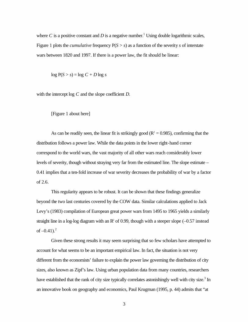
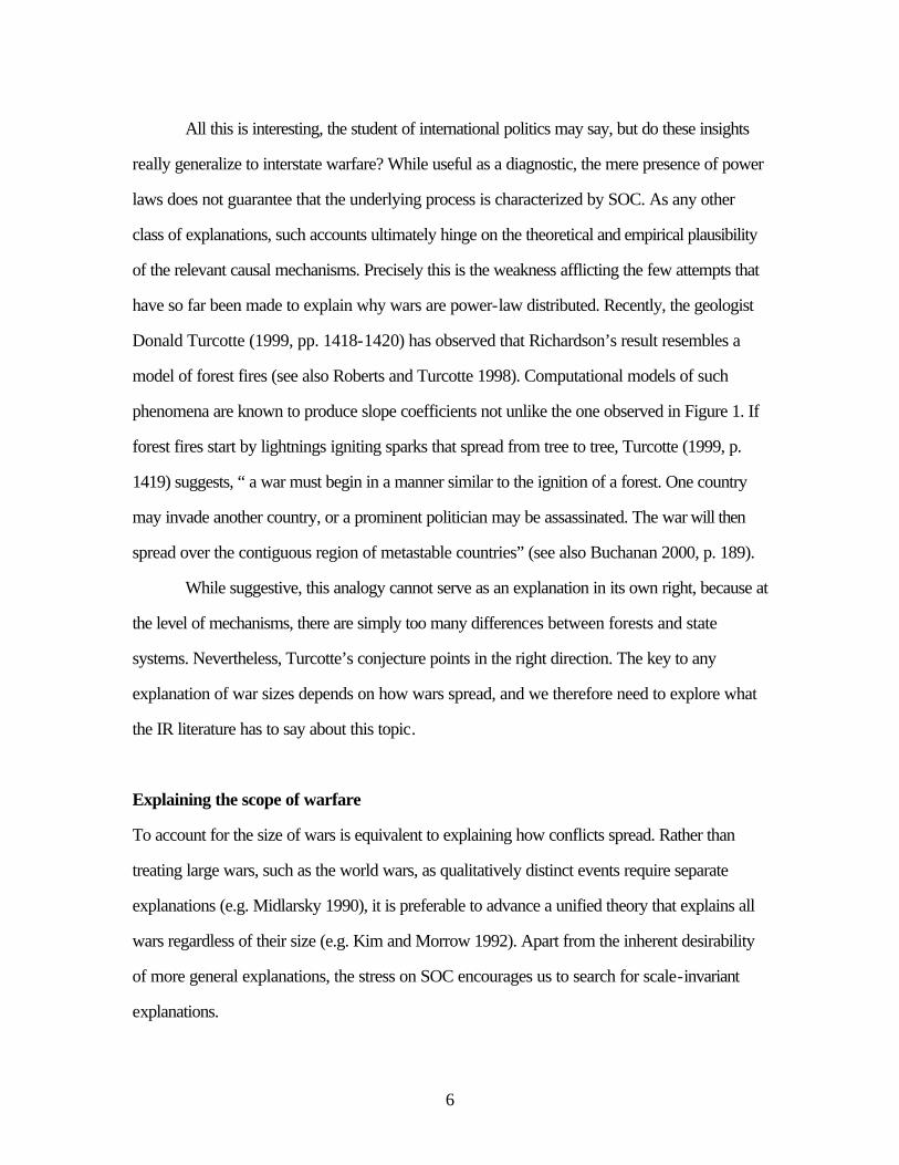
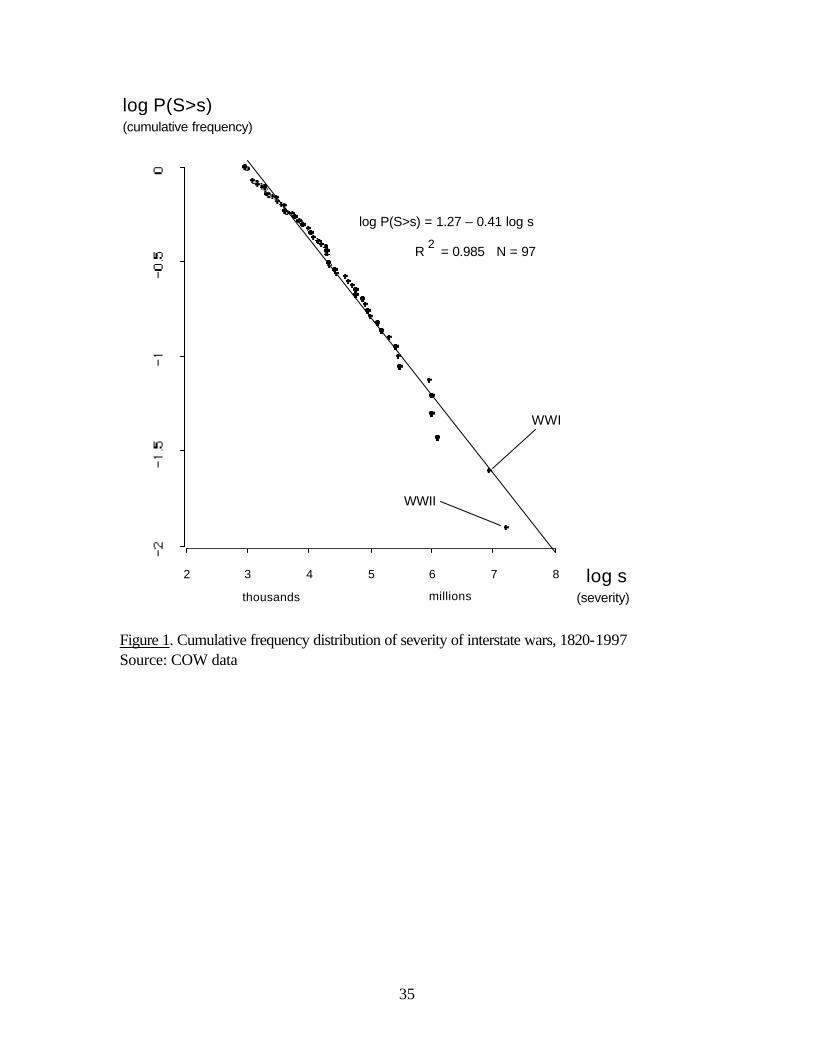
where C is a positive constant and D is a negative number.1 Using double logarithmic scales,

Figure 1 plots the cumulative frequency P(S > s) as a function of the severity s of interstate

wars between 1820 and 1997. If there is a power law, the fit should be linear:

log P(S > s) = log C + D log s

with the intercept log C and the slope coefficient D.

[Figure 1 about here]

As can be readily seen, the linear fit is strikingly good (R2 = 0.985), confirming that the

distribution follows a power law. While the data points in the lower right-hand corner

correspond to the world wars, the vast majority of all other wars reach considerably lower

levels of severity, though without straying very far from the estimated line. The slope estimate –

0.41 implies that a ten-fold increase of war severity decreases the probability of war by a factor

of 2.6.

This regularity appears to be robust. It can be shown that these findings generalize

beyond the two last centuries covered by the COW data. Similar calculations applied to Jack

Levy’s (1983) compilation of European great power wars from 1495 to 1965 yields a similarly

straight line in a log-log diagram with an R2 of 0.99, though with a steeper slope (–0.57 instead

of –0.41).2

Given these strong results it may seem surprising that so few scholars have attempted to

account for what seems to be an important empirical law. In fact, the situation is not very

different from the economists’ failure to explain the power law governing the distribution of city

sizes, also known as Zipf’s law. Using urban population data from many countries, researchers

have established that the rank of city size typically correlates astonishingly well with city size.3 In

an innovative book on geography and economics, Paul Krugman (1995, p. 44) admits that “at

4

this point we have to say that the rank-size rule is a major embarrassment for economic theory:

one of the strongest statistical relationships we know, lacking any clear basis in theory.”

By the same token, Richardson’s law remains an equally acute embarrassment to IR

theory. For sure, the law has been known for a long time, but the vast majority of researchers

have paid scant attention to it. For example, there’s no mention of it in Geller and Singer’s

(1998) comprehensive survey of quantitative peace research dating back several decades (see

also Midlarsky 1989; Vasquez 1993). Those scholars who have focused explicitly on the

relationship between war severity and frequency have found an inverse correlation, but have

typically not framed their findings in terms of power laws (e.g. Gilpin 1981, p. 216; Levy and

Morgan 1984).

To my knowledge there are extremely few studies that attack Richardson’s law head-

on.4 Given the discrepancy between the empirical findings and the almost complete absence of

theoretical foundations on which to rely to account for them, we are confronted with a classical

puzzle. This scholarly lacuna becomes all the more puzzling because of the notorious scarcity of

robust empirical laws in IR. Despite decades of concerted efforts to find regularities, why

haven’t scholars followed in the footsteps of Richardson, who, after all, is considered to be one

of the pioneers of quantitative analysis of conflict? Postponing consideration of this question to

the concluding section, I instead turn to a literature that appears to have more promise in

accounting for the regularity.

Scaling and self-organized criticality

Natural scientists have been studying power laws in various settings for more than a decade.

Usually organized under the notion of self-organized criticality (SOC), the pioneering

contributions by Per Bak and others have evolved into a burgeoning literature that covers topics

as diverse as earthquakes, biological extinction events, epidemics, forest fires, traffic jams, city

growth, market fluctuations, firm sizes, and indeed, wars (for popular introductions, see Bak

5

1996; Buchanan 2000). Alternatively, physicists refer to the key properties of these systems

under the heading of “scale invariance” (Stanley et al. 2000).

Self-organized criticality is the umbrella term that connotes slowly driven threshold

systems that exhibit a series of meta-stable equilibria interrupted by disturbances with sizes

scaling as power laws (Jensen 1998, p. 126; Turcotte 1999, p. 1380). In this context,

thresholds generate non-linearities that allow tension to build up. As the name of the

phenomenon indicates, there has to be both an element of self-organization and of criticality.

Physicists have known for a long time that, if constantly fine-tuned, complex systems, such as

magnets, sometimes reach a critical state between order and chaos (Jensen 1998, pp. 2-3;

Buchanan 2000, Chap. 6). What is unique about SOC systems, however, is that they do not

have to be carefully tuned to stay in the critical point where they generate the scale-free output

responsible for the power laws.5

Using a sandpile as a master metaphor, Per Bak (1996, Chap. 3) constructed a simple

computer model that produces this type of regularity (see Bak, Tang, and Wiesenfeld 1987;

Bak and Chen 1991). If grains of sand trickle down slowly on the pile, power-law distributed

avalanches will be triggered from time to time. This example illustrates the abstract idea of SOC:

a steady, linear input generates tensions inside a system that in turn lead to non-linear and

delayed output ranging from small events to huge ones.

Whereas macro-level distributions emerge as stable features of scale-free systems, at

the micro-level, such systems exhibit a strong degree of path-dependence (Arthur 1994;

Pierson 2000). To use the sandpile as an illustration, it matters exactly where and when the

grains land. This means that point prediction often turns out to be futile, as exemplified by

earthquakes. This does not mean, however, that no regularities exist. In particular, it is important

to distinguish complex self-organized systems of the SOC kind from mere chaos, which also

generates unpredictable behavior (Bak 1996, pp. 29-31; Axelrod and Cohen 1999, p. xv;

Buchanan 2000, pp. 14-15).

6

All this is interesting, the student of international politics may say, but do these insights

really generalize to interstate warfare? While useful as a diagnostic, the mere presence of power

laws does not guarantee that the underlying process is characterized by SOC. As any other

class of explanations, such accounts ultimately hinge on the theoretical and empirical plausibility

of the relevant causal mechanisms. Precisely this is the weakness afflicting the few attempts that

have so far been made to explain why wars are power-law distributed. Recently, the geologist

Donald Turcotte (1999, pp. 1418-1420) has observed that Richardson’s result resembles a

model of forest fires (see also Roberts and Turcotte 1998). Computational models of such

phenomena are known to produce slope coefficients not unlike the one observed in Figure 1. If

forest fires start by lightnings igniting sparks that spread from tree to tree, Turcotte (1999, p.

1419) suggests, “ a war must begin in a manner similar to the ignition of a forest. One country

may invade another country, or a prominent politician may be assassinated. The war will then

spread over the contiguous region of metastable countries” (see also Buchanan 2000, p. 189).

While suggestive, this analogy cannot serve as an explanation in its own right, because at

the level of mechanisms, there are simply too many differences between forests and state

systems. Nevertheless, Turcotte’s conjecture points in the right direction. The key to any

explanation of war sizes depends on how wars spread, and we therefore need to explore what

the IR literature has to say about this topic.

Explaining the scope of warfare

To account for the size of wars is equivalent to explaining how conflicts spread. Rather than

treating large wars, such as the world wars, as qualitatively distinct events require separate

explanations (e.g. Midlarsky 1990), it is preferable to advance a unified theory that explains all

wars regardless of their size (e.g. Kim and Morrow 1992). Apart from the inherent desirability

of more general explanations, the stress on SOC encourages us to search for scale-invariant

explanations.

7

Although most of the literature focuses on the causes of war, some researchers have

attempted to account for how wars expand in time and space (Siverson and Starr 1991). A

majority of these efforts center on diffusion through borders and alliances. Territorial contiguity

is perhaps the most obvious factor enabling conflictual behavior to spread (Vasquez 1993, pp.

237-240). Empirical evidence indicates that states that are exposed to “warring border nations”

are more likely to engage in conflict than those that are not (Siverson and Starr 1991, chap. 3).

Geopolitical adjacency in itself says little about how warfare expands, however. The main logic

pertains to how geopolitical instability changes the strategic calculations by altering the

contextual conditions: “An ongoing war, no matter what its initial cause, is likely to change the

existing political world of those contiguous to the belligerents, creating new opportunities, as

well as threats” (Vasquez 1993, p. 239; see also Wesley 1962).

The consensus among empirical researchers confirms that alignment also serves as a

primary conduit of conflict by entangling states in conflictual clusters (for references, see

Vasquez 1993, pp. 234-237). In fact, the impact of “warring alliance partners” appears to be

stronger than that of warring border nations (Siverson and Starr 1991). Despite the obvious

importance of alliances, however, I will consider contiguity only. Because of its simplicity, the

alliance-free scenario serves as a useful baseline for further investigations. Drawing on Vasquez’

reference to strategic context, I assume that military victory resulting in conquest changes the

balance-of-power calculations of the affected states. The conqueror typically grows stronger

while the weaker side loses power. This opens up new opportunities for conquest, sometimes

prompting a chain reaction that will only stop until deterrence or infrastructural constrains

dampen the process (e.g. Gilpin 1981; Liberman 1996).

What could turn the balance of power into such a period of instability? Clearly, the list

of sources of change is long, but here I will highlight one crucial class of mechanisms relating to

environmental factors. Robert Gilpin (1981, Chap. 2) asserts that change tends to be driven by

innovations in terms of technology and infrastructure. Such developments may facilitate both

resource extraction and power projection. In Gilpin’s words, “technological improvements in

8

transportation may greatly enhance the distance and area over which a state can exercise

effective military power and political influence” (p. 57).

As Gilpin (1981, p. 60) points out, technological change often gives a particular state

an advantage that can translate into territorial expansion. Yet, it needs to be remembered that

“international political history reveals that in many instances a relative advantage in military

technique has been short-lived. The permanence of military advantage is a function both of the

scale and complexity of the innovation on which it is based and of the prerequisites for its

adoption by other societies.” Under the pressure of geopolitical competition, new military or

logistical techniques typically travel quickly from country to country until the entire system has

adopted the more effective solution. It is especially in such a window of opportunity that

conquest takes place.

Going back to the sandpile metaphor, it is instructive to liken the process of

technological change with the stream of sand falling on the pile. As innovations continue to be

introduced, there is a trend toward formation of larger political entities thanks to the economies

of scale. If the SOC conjecture is correct, the wars erupting as a consequence of this

geopolitical process should conform with a power law.

Modeling geopolitics

How could we move from models of sandpiles and forest fires to more explicit formalizations of

war diffusion? Since the power law of Figure 1 stretches over two centuries, it is necessary to

factor in Braudel’s longue durée of history. But such a perspective raises the explanatory bar

considerably, because this requires a view of states as territorial entities with dynamically

fluctuating borders rather than as fixed billiard balls. Levy’s data, focusing on great power wars

in Europe, for example, coincides with massive rewriting of the geopolitical map of Europe. In

early modern Europe, there were up to half a thousand (more or less) independent geopolitical

units in Europe, a number that decreased to some twenty states by the end of Levy’s sample

period (Tilly 1975, p. 24; cf. also Cusack and Stoll 1990, Chap. 1).

9

It therefore seems hopeless to trace macro patters of warfare without endogenizing the

very boundaries of states. Fortunately, there is a family of models that does precisely that.

Pioneering agent-based modeling in IR, Bremer and Mihalka (1977) introduced an imaginative

framework of this type featuring conquest in a hexagonal grid, later extended and further

explored by Cusack and Stoll (1990). Building on the same principles, the current model, which

is implemented in the Java-based toolkit Repast (see http://repast.sourceforge.net), differs in

several respects from its predecessors.

Most importantly, due to its sequential activation of actors interacting in pairs that hard-

wires the activation regime, Bremer-Mihalka’s framework is not well suited to study the scope

of conflicts. By contrast, the quasi-parallel execution of the model presented here allows conflict

to spread and diffuse, potentially over long periods of time. Moreover, in the Bremer-Mihalka

configuration, combat outcomes concern entire countries at a time, whereas in the present

formalization, it affects single provinces at the local level. Without this more fine-grained

rendering of conflicts, it is difficult to measure the size of wars accurately.

The standard initial configuration consists of a 50 x 50 square lattice populated by about

200 composite, state-like agents interacting locally. Because of the boundary-transforming

influence of conquest, the interactions among states take place in a dynamic network rather than

directly in the lattice. In each time period, the actors allocate resources to each of their fronts

and then choose whether or not to fight with their territorial neighbors. While half of each state’s

resources is allocated evenly to its fronts, the remaining half goes to a pool of fungible resources

that are distributed in proportion to the neighbors’ power. This scheme assures that military

action on one front dilutes the remaining resources available for mobilization, which in turn

creates a strong strategic interdependence that ultimately affects other states’ decision-making.

An appendix describes this and all the other computational rules in greater detail.

For the time being, let us assume that all states use the same “grim-trigger” strategy in

their relations. Normally, they reciprocate their neighbors’ actions. Should one of the adjacent

actors attack them, they respond in kind without relenting until the battle has been won by either

10

side or ends with a draw. Unprovoked attacks can happen as soon as a state finds itself in a

sufficiently superior situation vis-à-vis a neighbor. Set at a ratio of three-to-one with respect to

the locally allocated resources, a stochastic threshold defines the offense-defense balance. An

identical stochastic threshold function determines when a battle is won.

Due to the difficulties of planning an attack, actors challenge the status quo with as low a

probability per period as 0.01. If fighting involves neighboring states, however, a contextual

activation mechanism prompts the state to enter alert status during which unprovoked attacks

are attempted in every period. This mechanism of contextual activation captures the shift from

general to specific deterrence in crises.6

When the local capability balance tips decisively in favor of the stronger party, conquest

results, implying that the victor absorbs the targeted unit. This is how hierarchical actors form. If

the target was already a part of another multi-province state, the latter loses its province.

Successful campaigns against the capital of corporate actors lead to their complete collapse.7

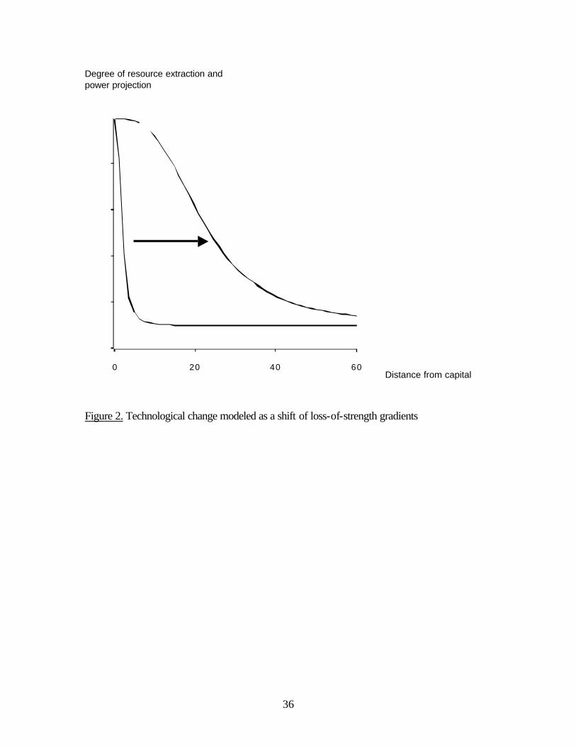
Territorial expansion has important consequences for the states’ overall resource levels.

After conquest, the capitals of conquered territories are able to “tax” the incorporated provinces

including the capital province. As shown in Figure 2, the extraction rate depends on the loss-of-

strength gradient that approaches one for the capital province but that falls quickly as the

distance from the center increases (Boulding 1963; Gilpin 1981, p. 115). Far away, the rate

flattens out around 10% (again see the appendix for details). This function also governs power

projection for deterrence and combat. Given this formalization of logistical constraints,

technological change is modeled by shifting the threshold to the right, a process that allows the

capital to extract more resources and project them power farther away from the center. In the

simulating runs reported in this paper, the transformation follows a linear process in time.

[Figure 2 about here]

11

Together all these rules entail four things: First, the number of states will decrease as the

power-seeking states absorb their victims. Second, as a consequence of conquest, the surviving

actors increase in territorial size. Third, decentralized competition creates emergent boundaries

around the composite actors. Fourth, once both sides of a border reach a point at which no one

is ready to launch an attack, a local equilibrium materializes. If all borders are characterized by

such balances, a global equilibrium emerges. Yet, such an equilibrium is meta-stable because,

decision making always involves an element of chance and, in addition, technological change

affects the geopolitical environment of the states.

An illustrative sample run

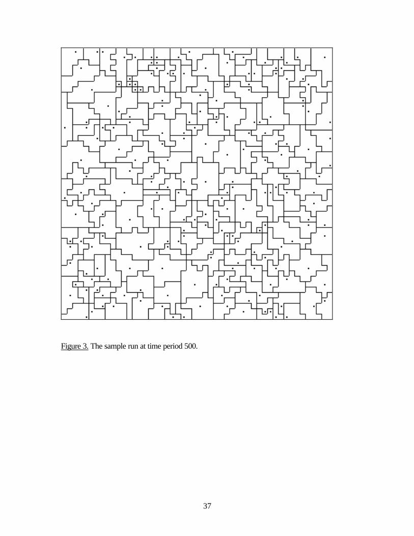
The experimental design features two main phases. In an initial stage until time period 500, the

initial 200 states are allowed to compete. Figure 3 shows a sample system at this point. The

lines indicate the states’ territorial borders and the dots their capitals. Because of some cases of

state collapse, the polarity has actually gone up to 205.

[Figure 3 about here]

After the initial phase, technological change is triggered and increases linearly for the rest

of the simulation until time period 10,500. At the same time, the war counting mechanisms is

invoked. The task of operationalizing war size involves two problems. First, spatio-temporal

conflict clusters have to be identified as wars. Once identified, their severity needs to be

measured. Empirical studies usually operationalize severity as the cumulative number of combat

casualties among military personnel (Levy 1983; Geller and Singer 1998). To capture this

dimension, the algorithm accumulates the total battle damage incurred by all parties to a conflict

cluster. The battle damage amounts to ten per cent of the resources allocated to any particular

front (see the appendix).

12

The question of identification implies a more difficult computational problem. In real

historical cases, empirical experts bring their intuition to bear in determining the boundaries of

conflict clusters. While it is not always a straight-forward problem to tell “what is a case” (Ragin

and Becker 1992), wars tend to be reasonably well delimited (though see Levy 1983, Chap.

3). In an agent-based model, by contrast, this task poses considerable problems because of the

lack of historical intuition. The model therefore includes a spatio-temporal cluster-finding

algorithm that draws a distinction between active and inactive states. Active states are those that

are currently fighting, or that fought in the last twenty time periods. The latter rule introduces a

“war shadow” that blurs the measurement so that briefs lulls in combat do not obscure the larger

picture. A cluster in a specific period is defined as any group of adjacent fighting states as long

as there is conflictual interaction binding them together. This allows for the merger of separate

conflicts into larger wars. The temporal connection is made by letting the states that are still

fighting in subsequent periods retain their cluster identification. Once there is no more active

state belonging to the conflict cluster, it is defined as a completed war and its accumulated

conflict count is reported.

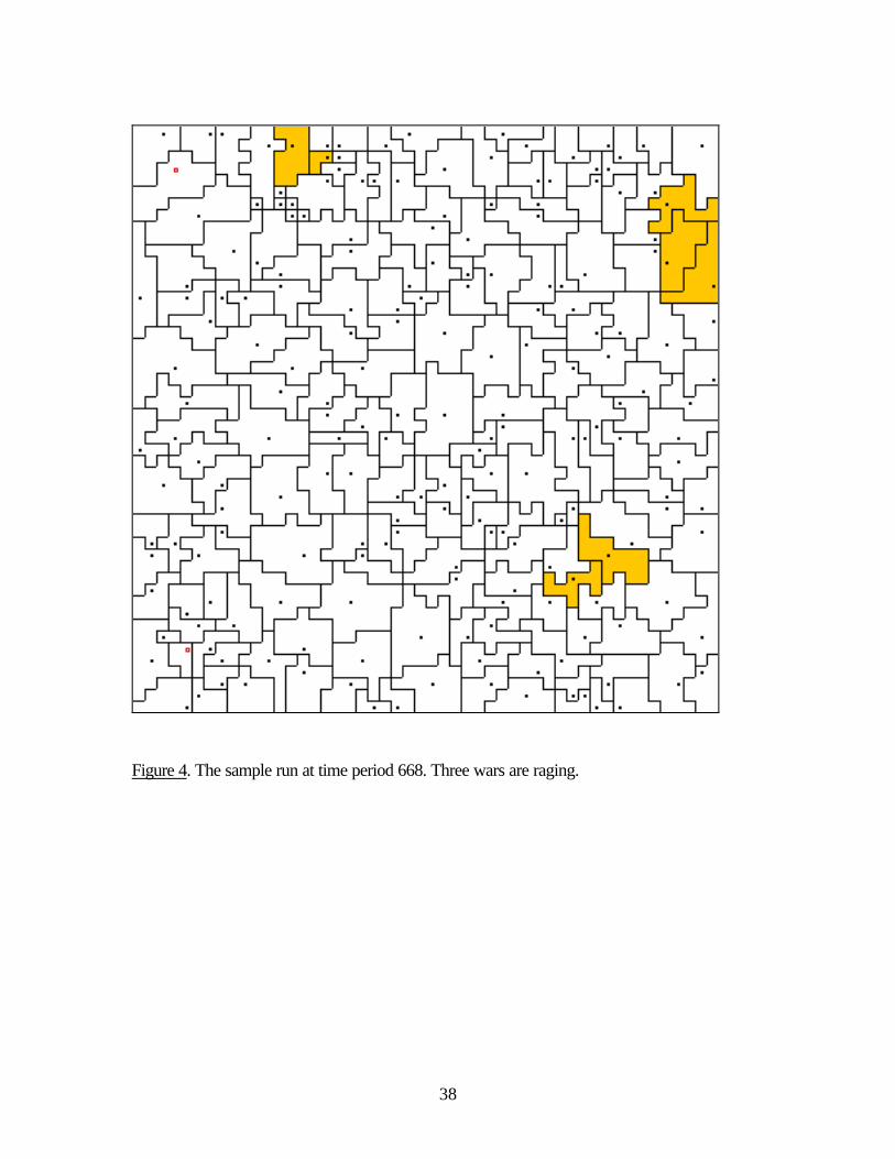
Figure 4 illustrates the sample system at time period 668. The three highlighted areas

correspond to conflict clusters that remained local. Whereas most conflicts involve two or three

actors, some engulf large parts of the system.

[Figure 4 about here]

The technological diffusion process starts acting as soon as the initial period is over, as

indicated by two the states with capitals marked as hollow squares in Figure 4. This process has

dramatic consequences over the course of the simulation. Figure 5 depicts the final configuration

of the sample run in time period 10,500. At this stage, there are only 35 states in the system

some of which have increased their territory considerably. Smaller states manage to survive

13

because, as a rule, they have fewer fronts to defend and are in some cases partly protected by

the boundary of the grid.

[Figure 5 about here]

Having explored the qualitative behavior of the model, it is time to address the question

of whether the model is capable of generating robust power laws.

Replications

We start by exploring the output of the illustrative run. Based on the same type of calculations as

in the empirical case, Figure 6 plots the cumulative frequency against corresponding war sizes. It

is clear that the model is capable of producing power laws with an impressive linear fit. In fact,

regression analysis produces an R2 of 0.991 that surpasses the fit of the empirical distribution

reported in Figure 1.8 Equally importantly, the size range extends over more than four orders of

magnitude, thus paralleling the wide region of linearity evidenced in the historical data.

Moreover, with a slope at –0.64, the inclination also comes close to empirically realistic levels.

[Figure 6 about here]

The choice of the sample system is not accidental. In fact, it is representative of a larger

set of systematic replications with respect to linear fit. More precisely, the illustrative run

corresponds to the medium R2 value of out a pool of fifteen artificial histories, that were

generated by varying the random seed that governs all stochastic events including the initial

configuration. Each replication lasted from time zero all the way to time period 10,500. As

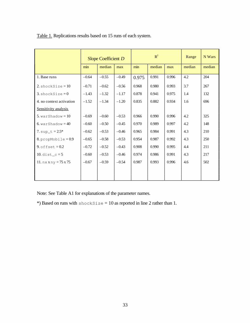
reported in line 1 of Table 1, regression analysis of these series yields 15 R2 values ranging from

0.975 to 0.996, with a median of 0.991 corresponding to the sample run. The table also reveals

that while the linear fit and the size range of this run are typical, its slope is far below the median

14

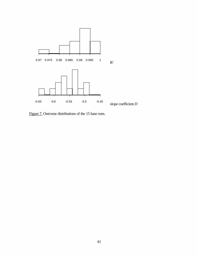
value of –0.55. As a complement, Figure 7 displays a summary of the replications findings in

graphical form. The upper histogram confirms that the linear fit of all the runs falls around the

median at 0.991. The slope distribution is somewhat more scattered, but it is not hard to discern

a smoother distribution describing the general behavior of the system.

[Table 1 about here]

[Figure 7 about here]

These are encouraging findings. Yet, establishing the presence of power laws in a small

set of runs is not the same thing as highlighting their causes. Therefore, we now turn to a set of

experiments that will help us find the underlying causes of the regularities.

What drives the results?

The previous section has shown findings based on one specific set of parameters. Table A1 in

the appendix reminds us that there are many knobs to turn. Indeed, the calibration process

turned out to be rather difficult. Given that war has been a rare event in the Westphalian system,

the trick is to construct a system that “simmers” without “boiling over” into perennial warfare.

This section presents a series of experiments that suggest that technological change and

contextual activation, rather than other factors, are responsible for the production of power

laws.

The easiest way of establishing the result relating technological change is to study a set

of counterfactual runs with less, or no, such transformations. Reflecting a loss-of-strength

gradient shifted 10 steps instead of 20, the runs corresponding to line 2 in Table 1 indicate that

the linearity becomes somewhat less impressive with a median R2 value at 0.980 and a less

expansive size range at 3.7. Furthermore, the median slope becomes as steep as –0.62. Once

the process of technological change is entirely absent, the scaling behavior disappears

15

altogether, as indicated by line 3. With a representative R2 at 0.941 and a range at 1.4, the

linear fit falls well short of what could be expected from even imperfect power laws.

Experiments with systems lacking contextual activation show that power-law behavior is unlikely

without this mechanism. In these runs, the linearity drops to even lower levels than without

technological change (see line 4).

These experiments confirm that technological change and contextual decision-making

plays a crucial role in generating progressively larger conflicts. However, the findings say little

about the general robustness of the scale-free output. It is thus appropriate to investigate the

consequences of varying other dimensions of the model. Keeping all other settings identical to

the base runs except for the dimension under scrutiny, lines 5 through 11 reveal that the power

laws generated in the base system are no knife-edge results. We start by testing whether the

granularity of the cluster-finding algorithm makes a difference. Lines 5 and 6 correspond to runs

with a “war shadow” set to 10 and 40 steps respectively, as opposed to the 20 steps used in

the base runs. While the linear fit does not change significantly in response to these tests, the

slope of the regression line in log-log space varies somewhat with the size of the smallest war

that can be detected. As would be expected, the finer the granularity, the steeper the line: as

opposed to a median slope of –0.55 in the base system, the coefficients become –0.60 and –

0.50 with war shadows at 10 and 40 respectively.

Does the location of the decision-making threshold for unprovoked attacks influence the

output? Line 7 reflects a series of runs in a system with the threshold sup_t set to 2.5 rather

than to 3 (see the appendix for the parameter notation). In order to prevent these runs from

degenerating into one big conflict cluster, the lower level of technological change of 10 was

chosen, but otherwise the settings were identical to those in the base runs. Again, fairly

impressive power laws emerge, in these cases with a median R2 of 0.984. The continued

sensitivity analysis reported in Line 8 increases the resource fungibility propMobile from 0.5

to 0.9 in the routine for resource allocation. As indicated by the table, this change does little to

alter the scaling behavior of the model.

16

Another set of tests pertain to distance dependence. Robustness checks with a higher

level of long-distance offset (line 9) and a steeper slope (line 10) produce outcomes similar to

those in the base model. Finally, the findings reported in line 11 indicate that the size of the grid

does not affect the process significantly. In fact, with an expanded 75 by 75 grid and

initPolarity = 450, the scaling behavior reaches an even higher level of accuracy with a

median R2 of 0.993 and a wider median range of 4.6. The slopes become somewhat steeper in

these larger systems.

Obviously, the point of the sensitivity analysis is not that the power laws hinge

exclusively on technological change and the contextual activation mechanism. It is not hard to

make the scale-free output vanish by choosing extreme values on any of the dimensions relating

to lines 5 to 11, or other parameters for that matter. Since finding this intermediate range of

geopolitical consolidation requires considerable parameter adjustment in the current model, the

pure case of parameter-insensitivity characterizing SOC cannot be said to have been fully

satisfied. Yet, the qualitative behavior appears to remain for a reasonably large range of values

and dimensions. Ultimately, extensive empirical calibration of the these parameters and

mechanisms will be required to reach an even firmer conclusion about the causes of

Richardson’s law.

In general terms, it is clear that scaling behavior depends on both a logistical “brake”

slowing down the states’ conquering behavior as well as on an “acceleration effect”, in this case

represented by the contextual activation mechanism. What self-correcting mechanisms could

render the scale-free behavior even less sensitive to parameter variations? It should be noted

that I have made a number of simplifying assumptions, which might render the computational

power laws less robust than they are in the real world. First of all, the attention must turn to

alliances since, as we have seen above, they have been singled out in the theoretical and

empirical literature on war diffusion. More generally, interaction has been restricted to

contiguous neighbors. Relaxing that assumption would allow great powers to extend their reach

17

far beyond the neighboring areas. Such a mechanism would help explain how large conflicts

spread.

At the structural level, it would be necessary to consider secession and civil wars. These

constrains could slow down positive-feedback cycles of imperial expansion through implosion.

The exclusive focus on local, contiguous combat assumes away far-reaching interventions by

great powers both on land and at sea. Moreover, there is also nationalism, which affects not

only the extractive capacity but also the boundaries of states through national unification and

secession.

Conclusion

Despite the complications introduced by parameter sensitivity, the fact remains that the model in

its present “stripped” form has fulfilled its primary purpose, namely that of generating power

laws similar to those observed in empirical data. The current framework may well be the first

model of international politics that does precisely that. In addition, we have found that

technological change and contextually activated decision-making go a long way toward

explaining why power laws emerge in geopolitical systems. Without these mechanisms, it

becomes very hard to generate scale-free war-size distributions. These findings take us one step

closer to resolving Richardson’s original puzzle first stated more than half a century ago. The

computational reconstruction of this regularity strengthens our confidence in the conjecture that

interstate warfare actually follows the principles of self-organized criticality. However, stronger

confidence does not equal conclusive corroboration, which is something that requires

considerably more accurate portrayal of the causal mechanisms generating the phenomenon in

the first place.

If we nevertheless assume that the SOC conjecture holds, important consequences for

theory-building in IR follow. By using the method of exclusion, we have to ask what theories are

capable of generating regularities of this type.9 Most obviously, the logic of SOC casts doubt on

static equilibrium theories as blue-prints for systemic theorizing. If wars emanate from

18

disequilibrium processes, then these theories’ narrow focus on equilibrium is misguided. It is not

hard to find the main reason for this ontological closure: micro-economic theory has served as

the dominant source of inspiration for theory-builders in IR, and this influence has grown

stronger with the surge of rational-choice research (Thompson 2000, p. 26).

At the level of general theorizing, Waltz (1979) epitomizes this transfer of analogies by

stressing the prevalence of negative feedback and rationality in history. Yet, if SOC is a correct

guide to interstate phenomena such as war, it seems less likely that static frameworks such as

that suggested by Waltz are the right place to start in future attempts to build systems theory. In

fact, his sweeping anarchy thesis remains too vague to be particularly helpful in explaining

particular wars or any aggregate pattern of warfare for that matter (Vasquez 1993).

This reasoning does not render realist analysis of warfare obsolete, however. What the

computational analysis does tell us, however, is that such theorizing needs to rest on explicitly

spatio-temporal foundations. In fact, Robert Gilpin’s (1981) analytical sketch of war and

change may offer a more fruitful point of departure than does Waltz. Partly anticipating the SOC

perspective, Gilpin (1981) advances a dialectical theory that interprets wars as releases of built-

up tensions in the international system: “As a consequence of the changing interest of individual

states, and especially because of the differential growth in power among states, the international

system moves from a condition of equilibrium to one of disequilibrium” (p. 14). Once the tension

has been accumulated, it will sooner or later be released, usually in a violent way: “Although

resolution of a crisis through peaceful adjustment of the systemic disequilibrium is possible, the

principal mechanism of change throughout history has been war, or what we shall call

hegemonic war” (p. 15). Yet, rather than adopting an exclusively revolutionary approach to

warfare, Gilpin realizes that most adjustments produce much smaller conflicts. By adopting an

explicit non-equilibrium focus, Gilpin anticipates SOC theory (see also Organski and Kugler

1980).

Viewed as a source of theoretical inspiration, then, the sandpiles of non-equilibrium

physics may prove more useful as master analogies than both the billiard balls of classical

19

physics and than the “butterfly effect” of chaos theory. Earthquakes, forest fires, biological

evolution, and other historically formed complex systems, serve as better metaphors for the

broad picture of world history than “ahistorical” pool tables or intractable turbulence. It may not

be a coincidence that scholars trying to make sense of historical disruptions have been prone to

use seismic analogies. According to John Lewis Gaddis’ (1992, p. 22) analysis of the end of the

Cold War, “[w]e know that a series of geopolitical earthquakes have taken place, but it is not

yet clear how these upheavals have rearranged the landscape that lies before us.”

Following in the footsteps of contemporary natural science, computational modeling

enables IR theory to move from such intriguing, yet very loose, analogies to detailed

investigations of how causal mechanisms interact in time and space. While “system effects” are

well understood by qualitative theorists (e.g. Jervis 1997), they have not been integrated into a

comprehensive theory. Most importantly, careful modeling may help us avoid the pitfalls of the

simplistic analogizing that has so often haunted IR theory. For example, a seismic analogy

supported by statistical parallels between wars and earthquake magnitudes could tempt realist

“pessimists” to conclude that wars are as unavoidable as geological events. Yet, such a

conclusion does not follow from SOC at all, for unlike continental plates, democratic security

communities can emerge. Whereas some areas of the world are prone to frequent outbreaks of

interstate violence, in others, catastrophic events are virtually unthinkable. But unlike continental

plates, the pacific regions are socially constructed features of the international system. As

conjectured by Immanuel Kant, the emergence of democratic security communities over the last

two centuries shows that the “laws” of geopolitics can be transcended.

If SOC provides an accurate guide to world politics, it can be concluded that disaster-

avoidance through the “taming” of Realpolitik by promoting defensive mechanisms or by

avoiding “bandwagoning behavior” may be as futile as hoping that the “new economy” will

prevent stock-market crashes from ever happening. In the long run, we may be willing to pay

the price of market upheavals to benefit from the wealth-generating effect of decentralized

markets. By contrast, it is less obvious that the world can afford to run the risk of catastrophic

20

geopolitical events, such as nuclear wars. The only safe way of managing security affairs is to

transform the balance of power into a situation of trust, which is exactly what happened

between France and Germany in the last half century. While nuclear calamities would further

vindicate Richardson’s law, there would be few people around appreciating the advances of

social science should the ostensibly “impossible” turn out to be just another huge low-probability

event.

21

Appendix: Detailed model specification

The model is based on a dynamic network of relations among states in a square lattice. Primitive

actors reside in each cell of the grid and can be thought of as the basic units of the framework.

Although they can never be destroyed, many of them do expand territorially. This also implies

that they can lose their sovereignty as other actors come to dominate them hierarchically.

All actors, whether primitive or compound, keep track of their geopolitical context with

the help of a portfolio holding all of their current relationships. These can be of three types:

• territorial relations point to the four territorial neighbors of each primitive actor (north,

south, west, and east).

• interstate relations refer to all sovereign neighbors with which an actor interacts.

• hierarchical relations specify the two-way link between provinces and capitals.

Whereas all strategic interaction is located at the political level, territorial relations

become important as soon as structural change happens. Combat takes place locally and results

in hierarchical changes that will be described below.

The order of execution is quasi-parallel. To this achieve this effect, the list of actors is

scrambled each time structural change occurs. The actors keep a memory of one step and thus

in principle make up a Markov process.

In addition to a model-setup stage, the main simulation loop contains five phases that

will be presented in the following. In the first phase, the actors’ resource levels are calculated. In

the second phase, the states allocate resources to their fronts followed by a decision procedure,

during which they decide on whether to cooperate or defect in their neighbor relations. The

interaction phase determines the winner of each battle, if any. Finally, the structural change

procedure carries out conquest and other border-changing transformations.

This appendix refers to the parameter settings of the base runs reported in line 1 of

Table 1. Table A1 provides an overview of all system parameters with alternative settings in

parentheses.

22

[Table A1 about here]

Model Setup

At the very beginning of each simulation, the square grid with dimensions nx = ny = 50 is

created and populated with a preset number of composite actors: initPolarity = 200. The

algorithm lets these 200 randomly located actors be the founders of their own compound

states, the territory of which is recursively grown to fill out the intermediate space until no

primitive actors remain sovereign.

Resource updating

As the first step in the actual simulation loop, the resource levels are updated. The simple

“metabolism” of the system depends directly on the size of the territory controlled by each

capital. It is assumed that all sites in the grid are worth a resource unit. A sovereign actor i

begins the simulation loop by extracting resources from all of its provinces. It accumulates a

share of these resources determined by a distance-dependent logistical function f (see Figure 2

above):

f(d,t) = offset + (1-offset)/{1+(d/dist_t(t))^-dist_c}

where 0 = offset = 1.0 sets the flat extraction rate for long distances. In all runs reported on

in this paper, it is fixed at 0.1. Technological change governs the initial location of the threshold

dist_t(t), which is a function of time t, and the slope by dist_c = 3 (higher numbers

imply a steeper slope). In order to simulate technological development, the threshold of the

distance function f(d,t) is gradually shifted outward starting as a linear function of simulation

time, where:

dist_t(t) = dist_t + (t-initPeriod)*shockSize

23

and dist_t = 2 and initPeriod = 500. The added displacement of the threshold

shockSize = 20 determines the final location of the threshold. This shift represents the state

of the art of technological change with which each state catches up with a probability pShock

= 0.0001 per time period. This probability is contextually independent of the strategic

environment.

In addition, the battle damage is cumulated for all external fronts (see the interaction

module below). Finally, the resources of the actor res(i,t) in time period t can be

computed by factoring in the new resources (i.e. the non-discounted resources of the capital

together with the sum of all tax revenue plus the total battle damage) multiplied by a fraction

resChange = 0.01. This small amount assures that the resource changes take some time to

filter through to the overall resource level of the state:

tax = 0 for all provinces j of state i do tax = tax + f(dist(i,j),t) totalDamage = 0 for all external fronts j do totalDamage = totalDamage + damage(j,i) res(i,t) = (1-resChange) * res(i,t-1) + resChange * (1 + tax - totalDamage)

Resource allocation

Before the states can make any behavioral decisions, resources must be allocated to each front.

For unitary states, there are up to four fronts, each one corresponding to a territorial relation.

Resource allocation proceeds according to a hybrid logic. A preset share of each actor’s

resources is considered to be fixed and has to be evenly spread to all external fronts. Yet, this

scheme lacks realism because it underestimates the strength of large actors, at least to the extent

that they are capable of shifting their resources around to wherever they are needed. The

remaining part of the resources, propMobile = 0.5, are therefore mobilized in proportion to

24

the opponent’s local strength and the previous activity on respective front. Fungible resources

are proportionally allocated to fronts that are active (i.e. where combat occurs), but also for

deterrent purposes in anticipation of a new attack. Allocation is executed under the assumption

that no more than one new attack might happen.

For example, a state with 50 mobile units could use them in the following way assuming

that the five neighboring states could allocate 10, 15, 20, 25, and 30 respectively. If the

previous period featured warfare with the second and fourth of these neighbors, these two

fronts would be allocated 15/(15+25) × 50 = 18.75 and 25 / (15+25) × 50 = 31.25. Under the

assumption that one more war could start, the first, third, and fifth states would be allocated

respectively: 10/(15+25+10) × 50 = 10, 20/(15+25+10) × 50 = 20, and 30/(15+25+10) × 50

= 30.

Formally, resource allocation for state i starts with the computation of the fixed

resources for each relationship j. A preset proportion of the total resources res are evenly

spread out across the n fronts:

fixedRes(i,j) = (1-propMobile) * res / n

The remaining part mobileRes = propMobile * res is allocated in proportion to the

activity and the strength of the opponents. To do this, it is necessary to calculate all resources

that were targeted at actor i:

enemyRes(i) = ?{j}{res(j,i)}

The algorithm of actor i’s allocation can thus be summarized:

for all relations j do in case enemyRes(i) = 0 then [actor not under attack] res(i,j) = fixedRes(i,j)+mobileRes in case i and j were fighting in the last period then

25

res(i,j) = fixedRes(i,j) + r(j,i)/enemyRes(i)*mobileRes

in case i and j were not fighting the last period then res(i,j) = fixedRes(i,j)+ r(j,i)/(enemyRes(i)+r(j,i))*mobileRes

Decisions

Once each sovereign actor has allocated resources to its external fronts, it is ready to make

decisions about future actions. This is done by recording the front-dependent decisions in the

corresponding relational list. As with resource allocation, this happens in quasi-parallel through

double-buffering and randomized order of execution. The contextual activation mechanism

ensures that the actors can be in either an active or inactive mode depending on the combat

activity of their neighbors. Normally, the states are not on alert, which means that they attempt

to launch unprovoked attacks with a probability pAttack = 0.01. If they or their neighboring

states becomes involved in combat, however, they automatically enter the alerted mode, in

which case they contemplate unprovoked attacks in every round. Once there is no more action

in their neighborhood, they reenter the inactive mode with probability pDeactivate = 0.1 per

round.

All states start by playing unforgiving “grim trigger” with all their neighbors. If the state

decides to try an unprovoked attack, a randomly chosen potential victim j’ is selected. In

addition, a battle-campaign mechanism stipulates that the aggressor retains the current target

state as long as there are provinces to conquer unless the campaign is aborted with probability

pDropCampaign = 0.2. This rule guarantees that the conquering behavior does not become

too scattered.

The actual decision to attack depends on a probabilistic criterion p(i,j’) which

defines a threshold function that depends on the power balance i’s favor (see below). If an

attack is approved, the aggressor chooses a “battle path” consisting of an agent and a target

province. The target province is any primitive actor inside j’ (including the capital) that borders

26

on i. The agent province is a province inside state i (including the capital) that borders on the

target. In summary, the decision algorithm of a state i can be expressed in pseudo-code:

Decision rule of state i:

for all external fronts j do if i or j played D in the previous period then act(i,j) = D else act(i,j) = C [Grim Trigger] if there is no action on any front and with pAttack or if in alerted status or campaign then if ongoing campaign against then select j’ = campaign else select random neighbor j’ with p(i,j’) do change to act(i,j’) = D [launch attack against j’] randomly select target(i,j’) and agent(i,j’) campaign = j’

The precise criterion for attacks p(i,j’) remains to be specified. The current

version of model relies on a stochastic function of logistic type. The power balance plays the

main role in this calculation:

bal(i,j’) = f(d,.) * res(i,j’)/{f(d’,.) * (res(j’,i)} .

where f(d, . ) is the time-dependent distance function described above and d and d’

the respective distance from the capitals of i and j to the combat zone (here the temporal

parameter is suppressed for simplicity of exposition). This discounting introduces distance-

dependence with respect to power projection. Hence, the probability can be computed as:

p(i,j’) = 1/{1+(bal(i,j’)/sup_t)^(-sup_c)}

27

where sup_t = 3.0 is a system parameter specifying the threshold that has to be transgressed

for the probability of an attack to reach 0.5, and sup_c a tunable parameter that determines

the slope of the logistic curve, which is set to 20 for the runs reported in this paper.

Interaction

After the decision phase, the system executes all actions and determines the consequences in

terms of the local power balance. The outcome of combat is determined probabilistically. If the

updated local resource balance bal(i,j’) tips far enough in favor of either side, victory

becomes more likely for that party. In the initial phase, the logistical probability function

q(i,j’)has the same shape as the decision criterion with the same threshold set at vic_t =

3 and with an identical slope: vic_c = 20:

q(i,j’) = 1/{1+(bal(i,j’)/vic_t)^-vic_c}

This formula applies to attacking states. In accordance with the strategic rule of thumb

that an attacker needs to be about three times as powerful than the defender to prevail, the

defender’s threshold is set to 1/vic_t = 1/3.

Each time-step of a battle can generate one of three outcomes: it may remain

undecided, one or both sides could claim victory. In the first case, combat continues in the next

round due to the grim-trigger strategy in the decision phase. If the defending state prevails, all

action is discontinued. If the aggressor wins it can advance a claim, which is processed in the

structural change phase.

The interaction phase also generates battle damage, which is factored into the overall

resources of the state as we saw in the resource updating module. If j attacks state i, the costs

incurred by j corresponds to propDamage = 10 % of j’s locally allocated resources: 0.1 *

res(j,i). The total size of a war is the cumulative sum of all such damage belonging to the

same conflict cluster.

28

Structural change

Structural change is defined as any change of the actors’ boundaries. This version of the

framework features conquest as the only structural transformation, but other extensions of the

modeling framework include secession and voluntary unification. Combat happens locally rather

than at the country level, as in Cusack and Stoll (1990). Thus structural change affects only one

primitive unit at a time. The underlying assumption governing structural change enforces states’

territorial contiguity in all situations. As soon as the supply lines are cut between a capital and its

province, the provinces becomes independent. Claims are processed in random order, which

executed conquests locking the involved units in that round.

The units affected by any specific structural claim are defined by the target(i,j)

province. If it is

• a unitary actor, then the entire actor is absorbed into the conquering state,

• the capital province of a compound state, then the invaded state collapses and all its

provinces become sovereign,

• a province of a compound state, then the province is absorbed. If, as a consequence of this

change, any of the invaded states’ other provinces become unreachable from the capital,

these provinces regain sovereignty.

29

References

Arthur, W. Brian. 1994. Increasing Returns and Path Dependence in the Economy. Ann

Arbor: University of Michigan Press.

Axelrod, Robert. 1979. “The Rational Timing of Surprise.” World Politics 31: 228-246.

Axelrod, Robert. 1997. The Complexity of Cooperation: Agent-Based Models of

Competition and Collaboration. Princeton: Princeton University Press.

Axelrod, Robert and Michael D. Cohen. 1999. Harnessing Complexity: Organizational

Implications of a Scientific Frontier. New York City: Free Press.

Axtell, Rorbert. 2000. “The Emergence of Firms in a Population of Agents.” Working Paper

99-03-019. Santa Fe Institute, New Mexico.

Bak, Per. 1996. How Nature Works: The Science of Self-Organized Criticality. New York:

Copernicus.

Bak, Per and Kan Chen. 1991. “Self-Organized Criticality.” Scientific American 264: 46-53.

Bak, Per, Chao Tang, and Kurt Wiesenfeld. 1987. “Self-Organized Criticality: An Explanation

of 1/f Noise.” Physical Review Letters 59: 381-384.

Boulding, Kenneth E. 1963. Conflict and Defense. New York: Harper and Row.

Bremer, Stuart A. and Michael Mihalka. 1977. “Machiavelli in Machina: Or Politics Among

Hexagons.” In Problems of World Modeling, ed. Karl W. Deutsch. Boston: Ballinger.

Buchanan, Mark. 2000. Ubiquity: The Science of History... or Why the World Is Simpler

Than We Think. London: Weidenfeld and Nicolson.

Cioffi-Revilla, Claudio, and Manus I. Midlarsky. forthcoming. “Highest-Magnitude Warfare:

Power Laws, Scaling, and Fractals in the Most Lethal International and Civil War.” In

Festschrift in Honor of J. David Singer, ed. Paul Diehl. Ann Arbor: University of

Michigan Press.

Cusack, Thomas R. and Richard Stoll. 1990. Exploring Realpolitik: Probing International

Relations Theory with Computer Simulation. Boulder: Lynnie Rienner.

30

Gaddis, John Lewis. 1992. "The Cold War, the Long Peace, and the Future." In The End of

the Cold War: Its Meaning and Implications, ed. Michael J. Hogan. Cambridge:

Cambridge University Press.

Geller, Daniel S. and J. David Singer. 1998. Nations at War: A Scientific Study of

International Conflict. Cambridge: Cambridge University Press.

Gilpin, Robert. 1981. War and Change in World Politics. Cambridge: Cambridge University

Press.

Hui, Victoria Tin-bor. 2000. “Rethinking War, State Formation, and System Formation: A

Historical Comparison of Ancient China (659-221 BC) and Early Modern Europe

(1495-1815 AD).” Ph. D. Dissertation, Columbia University.

Jensen, Henrik Jeldtoft. 1998. Self-Organized Criticality: Emergent Complex Behavior in

Physical and Biological Systems. Cambridge: Cambridge University Press.

Jervis, Robert. 1997. System Effects: Complexity in Political and Social Life. Princeton:

Princeton University Press.

Kim, Woosang and James D. Morrow. 1992. “When Do Power Shifts Lead to War?”

American Journal of Political Science 36: 896-922.

Krugman, Paul. 1995. Development, Geography, and Economic Theory. Cambridge, Mass.:

MIT Press.

Levy, Jack S. 1983. War in the Modern Great Power System, 1495-1975. Lexington:

Kentucky University Press.

Levy, Jack S. and T. Clifton Morgan. 1984. “The Frequency and Seriousness of War.”

Journal of Conflict Resolution 28: 731-749.

Liberman, Peter. 1996. Does Conquest Pay? The Exploitation of Occupied Industrial

Societies. Princeton: Princeton University Press.

Midlarsky, Manus I., ed. 1989. Handbook of War Studies. Boston: Unwin Hyman.

Midlarsky, Manus I. 1990. “Systemic Wars and Dyadic Wars: No Single Theory.”

International Interactions 16: 171-181.

31

Organski, A. F. K. and Jacek Kugler. 1980. The War Ledger. Chicago: University of Chicago

Press.

Pierson, Paul. 2000. “Increasing Returns, Path Dependence, and the Study of Politics.”

American Political Science Review 94: 251-267.

Ragin, Charles C. and Howard S. Becker, ed. 1992. What Is a Case? Exploring the

Foundations of Social Inquiry. Cambridge: Cambridge University Press.

Richardson, Lewis F. 1948. “Variation of the Frequency of Fatal Quarrels with Magnitude.”

American Statistical Association 43: 523-546.

Richardson, Lewis F. 1960. Statistics of Deadly Quarrels. Chicago: Quadrangle Books.

Roberts, D. C. and D. L. Turcotte. 1998. “Fractality and Self-Organized Criticality in Wars.”

Fractals 4: 351-357.

Siverson, Randolph M. and Harvey Starr. 1991. The Diffusion of War: A Study of

Opportunity and Willingness. Ann Arbor: The University of Michigan Press.

Stanley, H. E. et al. 2000. “Scale Invariance and Universality: Organizing Principles in Complex

Systems.” Physica A 281: 60-68.

Thompson, William R. 2000. The Emergence of the Global Political Economy. London:

Routledge.

Tilly, Charles. 1975. “Reflections on the History of European State-Making.” In The

Formation of National States in Western Europe, ed. Charles Tilly. Princeton:

Princeton University Press.

Turcotte, Donald L. 1999. “Self-Organized Criticality.” Reports on Progress in Physics 62:

1377-1429.

Vasquez, John A. 1993. The War Puzzle. Cambridge: Cambridge University Press.

Waltz, Kenneth N. 1979. Theory of International Politics. New York: McGraw-Hill.

Weiss, Herbert K. 1963. “Stochastic Models of the Duration and Magnitude of a ‘Deadly

Quarrel.” Operations Research 11: 101-121.

32

Wesley, James Paul. 1962. “Frequency of Wars and Geographic Opportunity.” Journal of

Conflict Resolution 6: 387-389.

33

Table 1. Replications results based on 15 runs of each system.

Slope Coefficient D

R2

Range N Wars

min median max min median max median

median

1. Base runs –0.64 –0.55 –0.49 0.975 0.991 0.996 4.2 204

2. shockSize = 10 –0.71 –0.62 –0.56 0.968 0.980 0.993 3.7 267

3. shockSize = 0 –1.43 –1.32 –1.17 0.878 0.941 0.975 1.4 132

4. no context activation –1.52 –1.34 –1.20 0.835 0.882 0.934 1.6 696

Sensitivity analysis

5. warShadow = 10 –0.69 –0.60 –0.53 0.966 0.990 0.996 4.2 325

6. warShadow = 40 –0.60 –0.50 –0.45 0.970 0.989 0.997 4.2 148

7. sup_t = 2.5* –0.62 –0.53 –0.46 0.965 0.984 0.991 4.3 210

8. propMobile = 0.9 –0.65 –0.58 –0.53 0.954 0.987 0.992 4.3 250

9. offset = 0.2 –0.72 –0.52 –0.43 0.908 0.990 0.995 4.4 211

10. dist_c = 5 –0.60 –0.53 –0.46 0.974 0.986 0.991 4.3 217

11. nx x ny = 75 x 75 –0.67 –0.59 –0.54 0.987 0.993 0.996 4.6 502

Note: See Table A1 for explanations of the parameter names.

*) Based on runs with shockSize = 10 as reported in line 2 rather than 1.

34

Table A1. System parameters in the geopolitical model.

System Parameters

Description

Values*

nx, ny dimensions of the grid 50 x 50 (75 x 75) initPolarity initial number of states 200 (450) initPeriod length of initial period 500 propMobile share of mobile resources to be allocated as

opposed to fixed ones 0.5 (0.9)

pDropCampaign probability of shifting to other target state after battle

0.2

pAttack probability of entering alert status 0.01 pDeactivate probability of leaving alert status 0.1 sup_t,sup_c superiority criterion (logistical parameters t

and c) 3.0, 20 (2.5, 20)

vic_t,vic_c victory criterion (logistical parameters t, c) 3.0, 20 (2.5, 20) propDamage share of damage inflicted on opponent 0.1 offset flat “tax rate” for long distances 0.1 (0.2) dist_t, dist_c loss-of-strength gradient (logistical

paramters t and c) 2, 3 (2, 5)

pShock probability of technological change 0.0001 shockSize final size of technological shocks 20 (0 & 10) warShadow period until next separate war can be

identified 20 (10 & 40)

*) The first values correspond to the base runs and the parenthesized ones to the other runs used in the sensitivity analysis (see Table 1).

35

2 83 4 5 6 7

log s (severity)

log P(S>s) (cumulative frequency)

WWI

WWII

thousands millions

log P(S>s) = 1.27 – 0.41 log s 2R = 0.985 N = 97

Figure 1. Cumulative frequency distribution of severity of interstate wars, 1820-1997 Source: COW data

36

Degree of resource extraction and power projection

0 6020 40Distance from capital

Figure 2. Technological change modeled as a shift of loss-of-strength gradients

37

Figure 3. The sample run at time period 500.

38

Figure 4. The sample run at time period 668. Three wars are raging.

39

Figure 5. The sample run at time 10500.

40

log Pr (S > s)

2 73 4 5 6log s

Figure 6. Simulated cumulative frequency distribution in the sample run.

41

0.97 10.975 0.98 0.985 0.99 0.995R2

-0.65 -0.45-0.6 -0.55 -0.5slope coefficient D

Figure 7. Outcome distributions of the 15 base runs.

42

Endnotes:

1 Power laws are also referred to as “1/f” laws since they describe events with a frequency

which is inversely proportional to their size (Bak 1996, pp. 21-24; Jensen 1998, p. 5). This is a

special case with D = –1.

2 The slope was estimated from severity 10,000 and above because Levy’s (1983) exclusion of

small-power wars would leads to under-sampling for low levels of severity. Preliminary analysis

together with Victoria Tin-bor Hui has yielded promising results for Ancient China, 659-221

BC despite very incomplete casualty figures (for data, see Hui 2000). In this case, the slope

becomes even steeper.

3 Since rank is closely linked to the c. d. f., this relationship is equivalent to the power laws

reported in Figure 1.

4 Among the exceptions, we find Cioffi-Revilla and Midlarsky (forthcoming) who suggest that

the power-law regularity applies not only to interstate warfare but also to civil wars (see also

Wesley 1962; Weiss 1963).

5 Yet, it is not required that SOC holds for any parameter values. As least to some extent, the

question of sensitivity depends on the particular domain at hand (Jensen 1998, p. 128).

6 As a way to capture strategic consistency, states retain the focus on the same target state for

several moves. Once it is time for a new campaign, the mechanism selects a neighbor randomly

7 Because the main rationale of the paper is to study geopolitical consolidation processes, the

current model excludes the possibility of secession (although this option has been implemented

in an extension of the model).

8 This analysis excludes war events that fall below 2.5 on the logarithmic scale, because the

clustering mechanism puts a lower bound on the wars that can be detected.

9 For a similar critique of conventional theorizing, see Robert Axtell (2000) who proposes a

simple model to account for power-law distributed firm sizes in the economy.