1

Modeling the Mechanical Properties of Solid State Orientation in Semi-Crystalline

Polymer Films: A Composite Theory Approach

D. Ryan Breese*

Department of Chemical and Materials Engineering, University of Cincinnati, Cincinnati, Ohio,

45221

Gregory Beaucage

Department of Chemical and Materials Engineering, University of Cincinnati, Cincinnati, Ohio,

45221

Synopsis

Controlling the extent of crystalline orientation is of great interest in polymer processing.

Orientation is effected by the choice of polymer, fabrication process, and processing conditions.

Where high degrees of uniaxial orientation are required, the polymer is typically oriented in a

solid state drawing process, where the polymer is stretched in a single direction at temperatures

below the melting point. During this process, pre-existing crystallites are transformed into rigid,

fiber-like structures with large aspect ratios. The presence of these rigid structures significantly

enhances the moduli and break strength of the polymer. This work presents a practical model

that explains the structural transformation of crystallites into fiber-like structures and predicts

physical properties based on the proposed volume fraction of fibers (ΦF). A connection can then

* Permanent Address: Polymer Research and Development, Lyondell Chemical Company, 11530

Northlake Dr., Cincinnati, Ohio, 45249

2

be formed between the polymer’s analytic characteristics, processing conditions and the final

engineering properties.

Introduction

Semi-crystalline polymers can be oriented to improve physical properties, such as the modulus

and tensile yield and break strengths. Several approaches have been proposed to explain the

molecular transitions that enhance these properties, but none are related to the inherent properties

of the polymer [1]. These transitional models include composites consisting of fibers of finite

length [2, 3], crystalline blocks connected with inter-crystalline tie molecules, that when oriented

form fibrillar structures [4], fibers whose aspect ratio increases during orientation [5], and

elaborate hierarchical systems consisting of fibrous structures on several length scales [6]. To

fully explain the structure-property relationship of oriented polymers, an adequate model must

incorporate the major structural transitions that occur during the orientation process. A

mechanical model that relates the inherent properties of the polymer to the structural changes is

valuable for understanding the characteristics of a polymer that relate to the enhancement in

physical properties. Such a model would be beneficial to a fundamental understanding of

structure property relationships and for use in polymer development for producing oriented films

with improved properties.

Transformational Model

Relating the Machine Direction Modulus to the Fiber Volume Fraction

A three component system consisting of fibers and a matrix of both amorphous and non-fiber

crystallites can be used to model drawn films. The non-fiber crystalline phase consists of

3

lamellar stacks with low uniaxial orientation of the c-axis and no extended chains [7]. The fiber

portion consists of both lamellae stacks with high uniaxial orientation of the c-axis and what few

lamellae that have unraveled to form extended chains [7, 8-10]. The components of the fiber

portion have a very large aspect ratio relative to those components of the non-fiber crystalline

portion so that the two phases are assumed to be easily distinguishable, both morphologically

and in terms of mechanical response.

The sum of the fractions of the non-fiber crystalline and fiber components is equivalent to the

percent crystallinity of the polymer, which is calculated by Equation (1):

)1(11

11

ac

a

C

!!

!!

"

"

=#

Where ΦC is the volume fraction crystallinity of the polymer, ρ is the density of the polymer

measured in a gradient column, ρa is the density of the amorphous polymer (0.885 g/cc) and ρc is

the density of the crystalline polymer (1.00 g/cc) [11]. When Φc = 0, ρ = ρa and when Φc =1, ρ =

ρc.

Due to the presence of branching and defects, the amorphous phase is unable to crystallize and

form fibrous structures, so only the polymer chains incorporated in the crystalline region

construct the non-fiber crystalline and fiber components [7]. The crystalline volume fraction is

then simply the sum of the volume fractions of the fiber and non-fiber crystalline phases.

)2(NFFC

!+!=!

Where ΦF is the volume fraction of fiber components and ΦNF is the volume fraction of non-fiber

crystalline components

4

From fiber composite theory, the following relationship is used to calculate the machine

direction modulus of a fiber composite system with fibers of an extremely large aspect ratio [12]:

)3(1

,, !=

"=n

i

iMDiMDCEE

Where E C,MD is the machine direction modulus of the composite, Ei, MD is the modulus of the ith

component in the machine direction, and Φi is the volume fraction of the ith component.

Halpin and Kardos [2] found that this model reasonable predicts the machine direction modulus

of the composite with fibers of aspect ratios greater than 103. By definition, Equation (3) is valid

for systems containing fibers that are perfectly oriented in the machine direction, have an

extremely large aspect ratio, and when no slippage occurs at the fiber-matrix interface. For the

case where the fiber aspect ratio is relatively small or interfacial slippage occurs, short fiber

composite techniques such as the Halpin-Kardos [2], Halpin-Tsai [3], and shear-lag based [4, 5]

theories could be considered.

In applications of fiber composite theory to semi-crystalline polymers, the main issue is

distinguishing which phase is the “fiber” and which is the “matrix”. The simplest approach

would be to attribute the crystalline region to the “fiber” and the amorphous region to the

“matrix” [10]. This is because in highly drawn, high crystalline polymers, the crystalline phase

is continuous throughout the sample, with the amorphous phase merely filling in the

imperfections. Moduli values between 240-345 GPa have been reported for the extended

polyethylene chain [5, 6, 13-15] and moduli values reported in the literature for the amorphous

region are of two to three orders of magnitude lower than that of the extended chain, and range

5

from 0.1-1 GPa [5, 6]. This means that at the elevated temperatures at which commercial

drawing processes operate, the amorphous region serves merely as a flexible medium, facilitating

the transformation of non-fiber crystallites into fibers. Due to the very low modulus of

amorphous polyethylene relative to crystalline polyethylene, the contribution of the amorphous

component in the composite can be omitted to greatly simplify the model into a dynamic two

component system consisting of fibers and non-fibrous crystallites transforming into fibers.

Omitting the minor contribution from the amorphous region to the machine direction modulus,

Equation (3) then becomes:

)4(,, NFNFMDFFMDCEEE !+!=

Substituting Equation (2) into Equation (4) provides:

)5()(,, FCNFMDFFMDCEEE !"!+!=

Limiting Moduli of the Transitional Model

As a polymer film is drawn, the modulus increases monotonically in draw ratio until failure due

to the conversion of non-fiber crystallites into fibrous structures. At failure, the entire non-fiber

crystalline region has been converted into fibers, resulting in the highest practically obtainable

modulus. This concept is supported by Peterlin [6], who states that the fracture of the drawn

sample in constant rate tensile experiments occurs almost instantaneously as soon as necking has

transformed the whole sample into a fibrous structure.

At this limiting condition, Equation (3) becomes:

)6(,,, MDFCMDFFMAXMDCEEE !"!=

6

This relationship provides a calculation of the machine direction modulus of the fiber, EF, MD, for

a given polymer and sample type, which is assumed to be constant with draw ratio [5].

Substituting EF, MD calculated from Equation (6) into Equation (5), we obtain the following

relationship between the machine direction modulus of a non-fiber crystalline/fiber composite

with respect to the fiber volume fraction.

)7()(,

, FCNF

C

MAXMDC

FMDCE

EE !"!+##

$

%&&'

(

!!=

Where EC,MD is the machine direction modulus of the composite, EC,MD MAX is the machine

direction modulus of the composite at the highest attainable draw ratio prior to failure, and ENF is

the modulus of the non-fibrous crystalline component of the composite matrix.

Relating the Transverse Direction Modulus to the Fiber Composition

From fiber composite theory [12], the following relationship is used to calculate the transverse

direction modulus of a composite system:

)8(1

1

,

!=

"=

n

i i

i

TDC

E

E

E C,TD is the transverse direction modulus of the composite, Ei is the modulus of the ith

component and Φi is the volume fraction of the ith component.

Utilizing Equations (2) and (8) and the previous arguments regarding the effects of the

amorphous phase, an equation for the two component system of fibers and non-fiber crystallites

is generated for the transverse direction modulus.

7

)9()(

1

,

,

NF

FC

TDF

F

TDC

EE

E!"!

+!

=

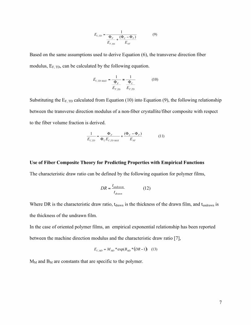
Based on the same assumptions used to derive Equation (6), the transverse direction fiber

modulus, EF, TD, can be calculated by the following equation.

)10(11

,,

,

TDF

C

TDF

F

MAXTDC

EE

E!

"!

=

Substituting the EF, TD calculated from Equation (10) into Equation (9), the following relationship

between the transverse direction modulus of a non-fiber crystallite/fiber composite with respect

to the fiber volume fraction is derived.

)11()(1

,, NF

FC

MAXTDCC

F

TDCEEE

!"!+

!

!=

Use of Fiber Composite Theory for Predicting Properties with Empirical Functions

The characteristic draw ratio can be defined by the following equation for polymer films,

)12(drawn

undrawm

t

tDR =

Where DR is the characteristic draw ratio, tdrawn is the thickness of the drawn film, and tundrawn is

the thickness of the undrawn film.

In the case of oriented polymer films, an empirical exponential relationship has been reported

between the machine direction modulus and the characteristic draw ratio [7],

( ) )13()1*exp(*, != DRBMEMDMDMDC

MM and BM are constants that are specific to the polymer.

8

Empirically, the transverse direction modulus is logarithmically related to the characteristic draw

ratio [7].

)14()ln(*, TDTDTDCMDRBE +=

MT and BT are constants that are specific to the polymer.

These empirical equations can be coupled with the transitional model (Equations (5, 7, 11)) to

predict both the machine and transverse direction moduli of the oriented film.

Problems with a Simple Model

The machine direction modulus of an oriented polymer film is proportional to the degree of

crystallinity (including both fibrous and non-fibrous crystalline components) and lamellar

thickness [7, 12, 16, 17]. At a specific draw ratio, EC,MD is primarily a function of molecular

orientation and fraction of crystallinity [10] and not heavily dependent on molecular weight [7].

Worth noting is that polymers with higher number average molecular weights are able to be

oriented to higher draw ratios, resulting in films with higher moduli values prior to the breaking

of the specimen [7, 10, 18]. The reason why the higher molecular weight polymers can be drawn

to higher ratios is likely due to this higher number of chain entanglements and the fewer number

of chain ends. The likelihood of the occurrence of a chain entanglement increases with

molecular weight [10], which increases the probability of two chains becoming intertwined and

unable to detangle without the application of an external force. Lower molecular weight

polymers also have more chain ends per unit volume, with the chain ends serving as a site for the

initiation of the catastrophic failure of the composite [15]. These small imperfections could

result in the failure of the film at the high tensile stress of the orientation process, considering the

9

fracture stress is proportional to the inverse square-root of the imperfection size from Griffith’s

theory on failure mechanics [19]. The effects of the chain ends on the maximum draw ratio are

amplified further in polymers with lower percent crystallinity. The difference between the

maximum draw ratios of polymers with the same degree of crystallinity, but different number

average molecular weights, increases with respect to decreasing polymer percent crystallinity.

Correlations between the polymers’ percent crystallinity and the transverse direction moduli are

similar to those discussed for the machine direction moduli. Polymers with higher percent

crystallinity obtain the highest transverse direction moduli.

Determining the Volume Fraction of Fibers from the Moduli of the Specimen

The transition model indicates that the mechanical properties of polymer films are determined by

ΦF, which is calculated by first combining Equations (7) and (13) for the machine direction:

( ))15(

)1*exp( ,

FC

MAXMDC

C

F

MDMD

NF

EDRBM

E!"!

##$

%&&'

(

!

!""

=

For the transverse direction modulus, Equations (11) and (14) are combined to yield:

( )

)16(

*)ln(*

1

)(

, !!"

#

$$%

&

''

(

)

**

+

,

-

-.

+

-.-=

MAXTDCC

F

TDTD

FC

NF

EMDRB

E

Equations (15) and (16) are then set equal to each other and the equation is solved for the fiber

volume fraction in the composite.

Discussion

10

This transition model is similar to that of Weeks and Porter [20] and Gibson, Davies, and Ward

[4] (which utilized Cox’s shear lag theory [21]), but is improved in the sense that the effects of

the orientation process on the modulus of the non-fiber crystalline component is incorporated

into the model by allowing a transition to fibers. In the case of Weeks and Porter’s sheath and

core model [19], they neglect any changes in the morphology of the sheath. When compared to

the short fiber model of Halpin-Kardos [2] or the shear lag based models of Gibson, Davies, and

Ward [4] and Barham and Arridge [5], knowledge of a finite aspect ratio of the fibers is

necessary, while changes in the “matrix” of the composite are ignored. In addition, once the

fibers are formed, further drawing does little to enhance that fiber’s contribution to the composite

[2]. The transition model is unique in that the enhancements in film properties are the direct

result of both the increase in the volume fraction of fibers and the enhancements in the properties

of the continuous phase. This is a result of the process of forming additional fibers through the

transformation of non-fiber crystallites into fibers. Previous methods neglect changes in the

matrix during the orientation process that significantly contribute to the physical properties of the

composite. This is overcome in the transitional model in a simple and usable way through

incorporating two equations for the non-fiber crystalline modulus derived from the machine and

transverse direction moduli (Equations (15) and (16)). Film stiffening occurs from the

transformation of the less rigid, non-fiber crystallites into fiber-like structures at low draw ratios,

which leaves the stiffer non-fiber crystallites in the continuous phase and results in a matrix with

overall higher moduli.

The transitional model proposes that as films are oriented, the amount of non-fiber crystallites

decrease due to their transformation into fibers, leaving the stiffer non-fiber crystallites that are

11

more resistant to transformation in the matrix. This results in an increase in the modulus of the

non-fiber crystalline phase and a decrease in the volume fraction of non-fiber crystallites with

increasing characteristic draw ratio. At low characteristic draw ratios, the less rigid non-fiber

crystallites are easily converted to fiber-like structures, while extremely high characteristic draw

ratios are needed to transform the stiffest of the non-fiber crystallites into fiber-like structures.

Model for ΦF and Comparison with the Transitional Model

While changes in the moduli of the transforming non-fiber crystallites are of definite interest, a

deeper understanding of the dynamics regarding how the fibers are formed with respect to the

changing draw ratios is of more importance. These fiber structures have significantly higher

moduli values [5-7, 13-15], and thus by Equation (4), play a larger role in the contribution to the

physical properties of the specimen as their volume fraction increases with higher draw ratio.

We can propose an activated rate law where ΦF, the volume fraction of fibers in the composite, is

a function of draw down ratio.

( ) )17()1(*exp* !"=" DRKFoF

Where Φo is the amount of fibers present in the undrawn polymer and KF is the rate constant for

the fiber formation process. The value of such an analysis is to correlate values for Φo and KF to

the characteristics of the polymers.

The rate of fiber formation is heavily influenced by the entangled high molecular weight portion

of the distribution, namely the breadth of the distribution and size of the higher molecular weight

polymer chains. Polymers with more entanglements have a greater interconnected network of

crystallites and are more resistant to small perturbations and are generally characteristic

12

polymers with higher average molecular weights [10]. As a result, increasing the amount of

entanglements within the polymer decreases the volume fraction of fibers at a given draw ratio as

a result of molecular mobility restrictions by the higher viscosity. At orientation temperatures

below the melting point of the polymer, it may be difficult to produce fibrous structures in

polymers with extremely high molecular weights (Mw > 1,000,000) by simple tensile drawing

[10]. Branching also affects the process of fiber formation. Low density and linear low density

polyethylenes, both of which have high levels of long and/or short chain branches that form

entanglements, typically can not for fibrous structures, even at elevated orientation temperatures

[22]. For these same reasons, films produced with polymers having significant molecular

entanglements will have lower volume fractions of fibers in an undrawn film.

Increasing Mz+1 increases the volume fraction of fibers at a given draw ratio and increases the

volume fraction of fibers in an undrawn film. This characteristic is the direct result of the

relaxation time being longer than the duration of the orientation process. These polymer behave

similarly in the extrusion process, where these chains retain more of the uniaxial orientation

induced by the die. In addition, increasing the breadth of the relaxation time spectrum by

increasing the breadth of the high end of the molecular weight distribution, indicated by ET [23],

decreases the volume fraction of fibers at a given draw ratio and decreases the rate at which the

fibers are formed throughout the drawing process.

Relating the Machine Direction Break Stress (σ*C, MD) and Strain (ε*

C, MD) to the Volume

Fraction of Fibers

13

From fiber composites [12], the following relationship is used to calculate the machine direction

break stress:

)20(1

*,

* !=

"=n

i

iiMDC ##

Where σ*C,MD = composite machine direction break stress, σ*

i = break stress of the ith component,

and Φi = volume fraction of the ith component.

Based on the earlier assumption that the amorphous region does not contribute significantly to

the overall strength of the composite, relative to the crystalline region, Equation (20) simplifies

to:

)21(**,

*

NFNF

FFMDC !+!= """

Substituting Equation (2) into Equation (21), the composite break strength is obtained in terms of

the volume fractions of fiber-like structures present in the composite.

)22()(**,

*

FCNFF

FMDC !"!+!= ###

As with the moduli, a close relationship is seen between the percent crystallinity and the break

stress of the polymers [10].

From fiber composite theory, the machine direction break strain of a composite is [12]:

)23(**,

*NFFMDC !!! ==

Where ε* C,MD is the composite machine direction break strain, ε* F is the break strain of the fiber,

and ε*NF is the break strain of the non-fiber crystallites at the break stress of the fiber.

14

For Equation (23), the composite will only deform to the extent that the fiber can elongate.

Beyond this point, the fiber breaks and the composite fails due to the significantly lower break

strength of the more flexible lamellar and amorphous regions [7].

For oriented polymers, a deviation from this concept is observed at low fiber volume fractions

[7]. For Equation (23) to be valid, the assumption must be made that perfect bonding exists

between the components of the composite, in this case the fiber, non-fiber crystalline, and

amorphous regions. This means that no slippage can occur at the interface between the phases.

The deviation from Equation (23) at low fiber volume fractions is likely the result of interfacial

slippage between the few fibers that are present, the non-fiber crystalline and the amorphous

regions. In addition, the flexibility of the amorphous region dominates at lower draw ratios,

allowing for more energy to be absorbed by this phase. This would not be the case with highly

drawn systems where the deformation of the amorphous region is significantly hindered by the

presence of rigid fibrous structures. At moderate characteristic draw ratios, an ample amount of

fibers have been generated where they dominate the tensile properties and control the

extensibility of the specimen. Beyond this “critical volume fraction of fibers”, all of the samples

produced from similar polymers [7] converge upon a uniform, very low machine direction break

strain. A relatively low machine direction break elongation is expected when the fibers

generated by the drawing process dominate the tensile properties of the composite [7].

Conclusions

This discussion has presented a model and empirical functions for understanding the effects of

uniaxial drawing on various physical properties of semi-crystalline polymers. The model

15

predicts the linear relationship between the moduli and break strength to the volume fraction of

fibers of an infinitely long fiber composite.

The model suggests that the machine direction modulus increases exponentially with respect to

the characteristic draw ratio until all crystals are converted into fiber-like structures. This

translates to a linear relationship between the machine direction modulus and the volume fraction

of fibers present in the structure. The relationship between the machine direction modulus and

the volume fraction of fibers follows fiber composite theory and is shown in Equation (3)

The transverse direction modulus increases logarithmically with respect to draw ratio until all

lamellae are converted into fiber structures. This translates to a linear relationship between the

transverse direction modulus and the inverse of the volume fraction of fibers. The relationship

between the transverse direction modulus and the volume fraction of fibers following fiber

composite theory is shown in Equation (8).

The machine direction break stress, increases exponentially with respect to the characteristic

draw ratio until all crystals are converted into fiber structures, indicating a linear relationship

between the machine direction break stress and the volume fraction of fibers present in the

structure consistent with composite theory, Equation (21). The machine direction break stress

conforms to fiber composite theory, represented in Equation (23), after a critical volume fraction

of fibers are generated. Below this critical volume fraction of fibers, the break elongation is

dominated by the less rigid non-fibrous crystallites and amorphous regions.

16

In addition, a relationship describing an activated process has been presented in Equation (17)

that explains the process of formation of fibrous structures and relates the volume fraction of

fibers to inherent characteristics of the polymer. Such information could be utilized to

synthesize new polymers that provide unique properties when oriented in the solid state.

17

References

1. Breese, D. R., Beaucage, G., Current Opinions in Materials Science, submitted (2005).

2. Halpin, J. C., Kardos, J. L., Journal of Applied Physics, 45, 5, 2235 (1972).

3. Ashton, J. E. , Halpin, J. C., Petit, P. H., Primer on Composite Materials Analysis, Technomic,

Stamford, Conn. (1969).

4. Gibson, A. G., Davies, G. R., Ward, I. M., Polymer, 19, 683 (1978).

5. Barham, P. J., Arridge, R. G. C., Journal of Polymer Science, Polymer Physics Edition,

15, 1177 (1977).

6. Peterlin, A., Advan. Chem. Ser., 142, 1 (1975).

7. Breese, D. R., Masters of Science Thesis, University of Cincinnati (2005).

8. Tagawa, T., Journal of Polymer Science, 18, 971, (1980).

9. Matsumoto, T., Kawai, T., Maeda, H., Die Makromolekulare Chemie, 107, 250, (1967).

10. Peacock, A. J., Handbook of Polyethylene Structures, Properties, and Applications, Marcel

Dekker, Inc., 2000.

11. Brandrup, J., Immergut, E. H., “Polymer Handbook”, John Wiley & Sons, Inc. (1966).

12. Agarwal, B. D., Broutman, L. J., “Analysis and Performance of Fiber Composites”, John

Wiley & Sons, Inc. (1990).

13. Ward, I. M., Plastics and Rubber Processing and Applications, 4, 77 (1984).

14. Karasawa, N., Dasgupta, S., Goddard, W. A., J. Phys. Chem., 95, 2260 (1991).

15. Crist, Buckley. Annual Review of Materials Science, 25, 295 (1995).

16. Bassett, D. C., Carder, D. R., Philosophical Magazine, 28, 3, 535, (1973).

17. Krigbaum, W. R., Roe, R. J., Smith, K. J., Polymer, 5, 3, 533, (1964).

18. Kalb, B., Pennings, A. J., Journal of Material Science, 15, 2584, (1980).

18

19. Young, R. J., Lovell, P. A., Introduction to Polymers, Chapman & Hall, London, (1991).

20. Weeks, N. E., Porter, R. S., Journal of Polymer Science, Polymer Physics Edition, 12, 635

(1974).

21. Cox, H. L., British Journal of Applied Physics,3, 72 (1952).

22. Araimo, L, De Candia, F., Vittoria, V., Peterlin, A., Journal of Polymer Science, Polymer

Physics Edition, 16, 2087 (1978).

23. Shroff, R., Mavridis, H., Journal of Applied Polymer Science, 57, 1605 (1995).

Table of Terms

Term Definition Units

ΦC volume fraction crystallinity of the polymer

ρ density of the polymer g/cc

ρa density of the amorphous polymer 0.885 g/cc [2]

ρc density of the crystalline polymer 1.00 g/cc [2]

ΦF volume fraction of fiber components

ΦNF volume fraction of non-fiber crystalline components

E C,MD machine direction modulus of the composite GPa

Ei, MD modulus of the ith component GPa

Φi volume fraction of the ith component

EF. MD modulus of the fiber component in the machine direction GPa

ENF modulus of the non-fiber crystalline component GPa

E C,MD Max machine direction modulus of the composite at the maximum

machine direction orientation GPa

19

E C,TD transverse direction modulus of the composite GPa

EF. TD modulus of the fiber component in the transverse direction GPa

E C,TD Max transverse direction modulus of the composite at the maximum

machine direction orientation GPa

DR characteristic draw ratio

tundrawn undrawn film gauge µm

tdrawn drawn film gauge µm

MMD modulus of undrawn film in the machine direction GPa

BMD rate constant for machine direction modulus relationship to draw

ratio

MTD modulus of undrawn film in the transverse direction GPa

BTD rate constant for transverse direction modulus relationship to

draw ratio

σ*C,MD composite machine direction break stress GPa

σ*i break stress of the ith component GPa

σ*F break stress of the fiber component GPa

σ*NF break stress of the non-fiber crystalline component GPa

ε*C,MD composite machine direction break strain %

ε*F break strain of the fiber component %

ε*NF break strain of the non-fiber crystalline component %