Modeling the largest gas field in North America with aid of neural networks

Hugoton and Panoma Fields, Kansas and Oklahoma

Martin K. DuboisGeoffrey C. Bohling

upscale porosityEECS 833, spring, 2006

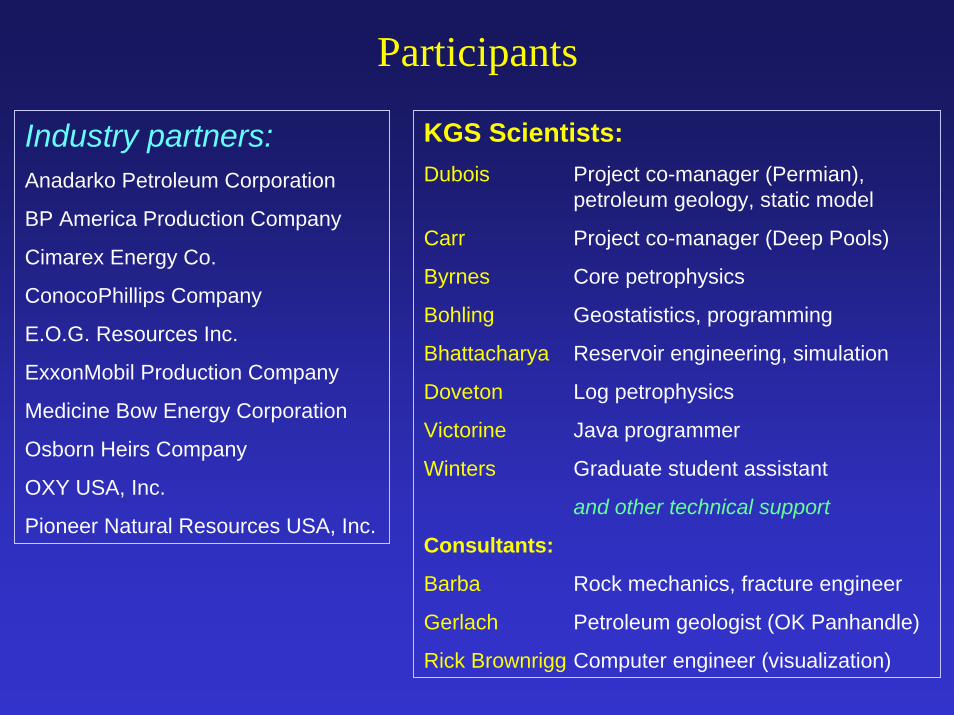
Participants

KGS Scientists:Dubois Project co-manager (Permian),

petroleum geology, static model

Carr Project co-manager (Deep Pools)

Byrnes Core petrophysics

Bohling Geostatistics, programming

Bhattacharya Reservoir engineering, simulation

Doveton Log petrophysics

Victorine Java programmer

Winters Graduate student assistant

and other technical support

Consultants:

Barba Rock mechanics, fracture engineer

Gerlach Petroleum geologist (OK Panhandle)

Rick Brownrigg Computer engineer (visualization)

Industry partners:Anadarko Petroleum Corporation

BP America Production Company

Cimarex Energy Co.

ConocoPhillips Company

E.O.G. Resources Inc.

ExxonMobil Production Company

Medicine Bow Energy Corporation

Osborn Heirs Company

OXY USA, Inc.

Pioneer Natural Resources USA, Inc.

To be covered

Today:• Model building workflow• Rock facies (basic building

blocks) and associated predictor variables

• Neural network structure• Nature of overlapping

feature space• Modeling results

Purpose of project:

Build geologic model to help optimize the field’s gas production

Model Dimensions:XY = 660’Z = 2-5’ mean (variable)77x130 miles10, 100 sq mi169 layersX = 618 rowsY = 1040 columns108 million cells

Small portion of model

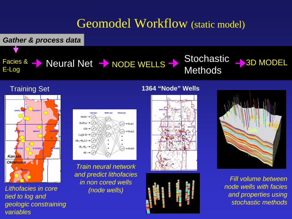
Geomodel Workflow (static model)

Facies & E-Log

Neural Net NODE WELLS StochasticMethods

3D MODEL

1364 “Node” Wells

Lithofacies in core tied to log and geologic constraining variables

Train neural network and predict lithofacies

in non cored wells (node wells)

Fill volume between node wells with facies

and properties using stochastic methods

Training Set

Gather & process data

Lithofacies from Core to “Node” Wells

Training set for neural network lithofacies prediction

Lithofacies predicted at 1369 “node wells”

Current training setOther

Some wells have both Chase and Council Grove core

80 mi130 km

130 mi

210 km

27 m

i43

km

Vertical well profilePredictor variables (feature elements) for a 250-foot (75 m) portion of Council Grove Group. Illustrated are five wire line log curves: gamma ray (GR), resistivity (ILD), photoelectric effect (PE), neutron-density porosity difference (DELTAPHI), and average neutron-density porosity (PHIND); and two geologic constraining variables: nonmarine-marine indicator (NM-M) and relative position (RPOS). Variables sampled at half-foot (0.15m) intervals are plotted against depth. Color indicates assigned facies, two are of continental origin, coarse siltstone (1) and shaleyfine siltstone (2), and six are of marine origin, marine siltstone (3), carbonate mudstone (4), wackestone (5), fine-crystalline dolomite (6), packstone (7), and grainstone (8). Formation or member level tops mark boundaries of marine and continental half-cycles.

Council Grove

Lithofacies

Tidal Flat

Co astal Pl ain

Lagoo

n

Ph yl. Algal M ound

Ide aliz ed De pos ition al Mo del (Mo dified a fter Rese rvoirs, I nc.)

100’s KM (1 00’s M iles)

(time slice)

Close-up Core Slab

0.5 mm

Thin Section Photomicrograph

M-CG Oncoid-PeloidPackstone

Cm21.2%32.3 md

L7

0.5 mm

Thin Section Photomicrograph

Close-up Core Slab

Dolomite13.9%1.1 md

Cm

L6

Thin Section Photomicrograph

0.5 mm L8

Pellet Grainstone

Close-up Core Slab

13.0%2.53 md

Phyloid Algal Bafflestone

20.6%1141 md

Core Slab

L8 0.5 mm

Thin Section Photomicrograph

Nonmarine Crs Siltstone-vfg SS

10.8%0.30 md

Close-up Core Slab

L0

Nonmarine Shaly Siltstone

Core Slab

Cm

0.5 mm

T h i n S e c t i o n Photomicrograph

4.6%0.000024 md

L1-2

0.5 mm Close-up Core Slab

Thin Section Photomicrograph Skeletal Wackestone

2.1%0.11 md

L5

10.4 %0.01 md

Core Slab

Marine Siltstone

0.5 mm

Thin Section Photomicrograph

L3

0.5 mm

Thin Section Photomicrograph

L4

Silty WackestoneCore Slab

3.4%0.0024 md

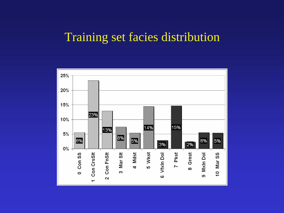
Training set facies distribution

Prepare data for model input1. Prepare 7 predictor variables:

Log curves: GR, ILD, N-Dphi, AvgNDphi, PE Geologic constraining variables (RelPos and NM-M by batch process)

2. Optimize NNet parameters (dampingparameter and # nodes in hidden layer) by cross validation exercises

3. Train and test neural networks4. Batch process lithofacies predictions5. Add lithofacies curves to predictor variable set6. Batch process porosity corrections (based on lithofacies)7. Generate LAS files for import to Petrel (Lithofacies and PhiCorr)

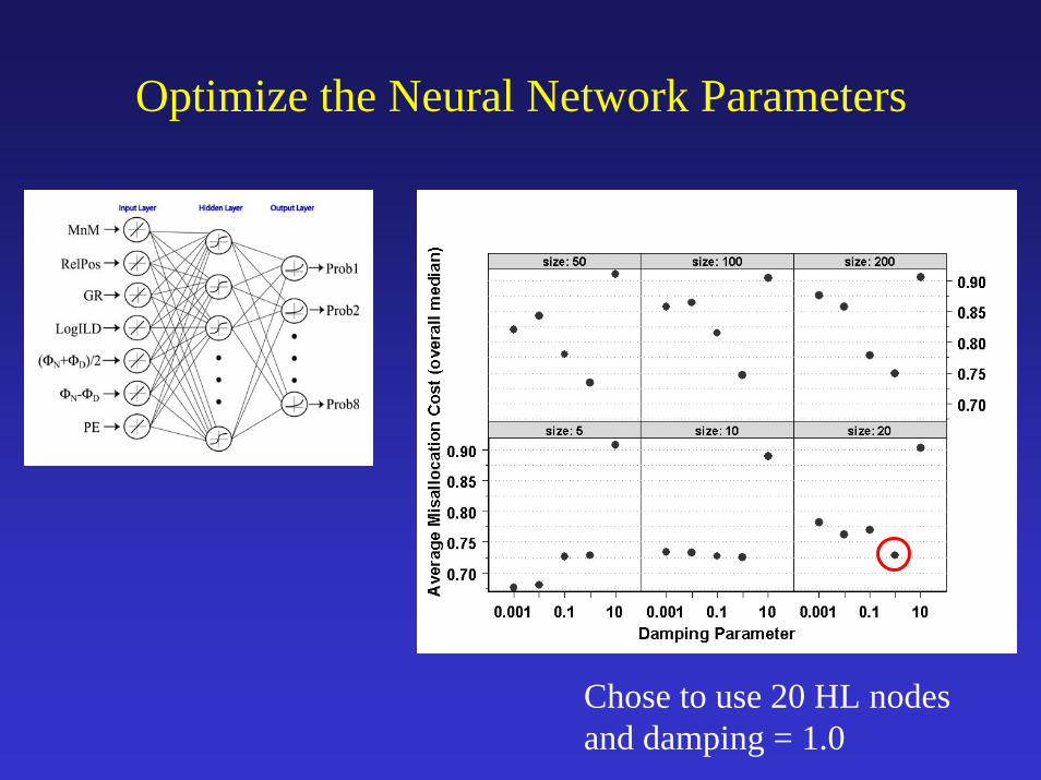
Optimize the Neural Network Parameters

Chose to use 20 HL nodes and damping = 1.0

Vertical succession of lithofacies

Regular vertical succession of facies (colors) is a result of oscillating sea level in response to glacial-interglacial cycles.

GR NM-MRelPos ILD PE DeltaPHI PHIND Seven predictor variables• RelPos and NM-M are derived

from formation tops information and serve to constrain the geology.

• Other variables are measured wireline log properties

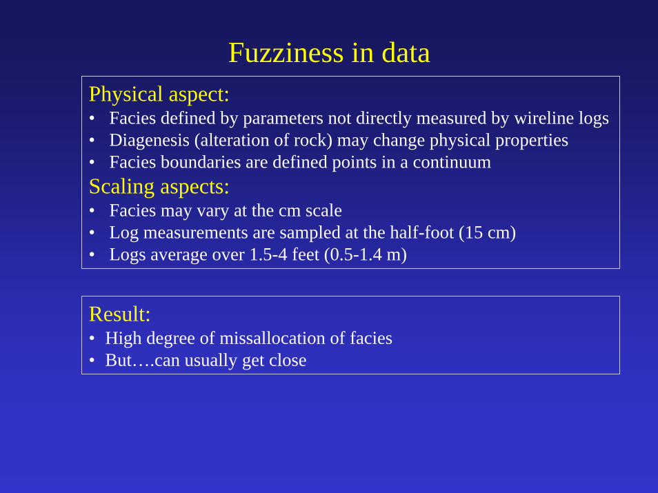
Fuzziness in dataPhysical aspect:• Facies defined by parameters not directly measured by wireline logs• Diagenesis (alteration of rock) may change physical properties• Facies boundaries are defined points in a continuumScaling aspects:• Facies may vary at the cm scale• Log measurements are sampled at the half-foot (15 cm)• Logs average over 1.5-4 feet (0.5-1.4 m)

Result:• High degree of missallocation of facies• But….can usually get close

Feature space

Cross plot of three of seven elements of data feature space (PE, Porosity andLogGR). Facies represented by colored dots form overlapping clouds in 3D space and are difficult to separate with parametrically defined boundaries

Cross plot of canonical variance scores. Facies represented by colored dots form overlapping clouds, but do exhibit clustering.

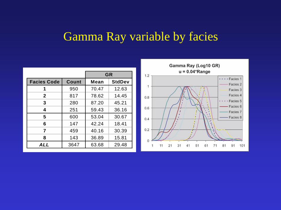
Gamma Ray variable by facies

Facies Code Count Mean StdDev1 950 70.47 12.632 817 78.62 14.453 280 87.20 45.214 251 59.43 36.165 600 53.04 30.676 147 42.24 18.417 459 40.16 30.398 143 36.89 15.81

ALL 3647 63.68 29.48

GR

Density functions

Density functions by class (k=8) for six of seven variables (j) using kernel density function with “optimal” smoothing window (u) for each variable. Facies key in first plot applies to all plots. Each variable has a unique feature space for each facies, although there is considerable overlap.

Feature vector statistics by element

Facies Code Count Mean StdDev Mean StdDev Mean StdDev Mean StdDev Mean StdDev1 950 70.47 12.63 12.84 3.78 5.58 4.66 3.21 0.38 3.72 1.352 817 78.62 14.45 16.18 5.19 6.81 5.78 3.30 0.49 3.85 1.283 280 87.20 45.21 11.77 3.03 6.05 3.62 3.73 0.49 6.27 2.094 251 59.43 36.16 8.58 3.38 5.17 3.92 4.09 0.54 7.86 2.985 600 53.04 30.67 7.90 3.31 2.96 3.51 4.25 0.64 8.30 4.606 147 42.24 18.41 13.01 4.69 6.30 3.93 3.77 0.56 3.30 1.597 459 40.16 30.39 9.03 4.08 2.37 3.78 4.61 0.66 8.76 7.808 143 36.89 15.81 10.50 4.36 1.22 6.41 4.44 1.00 6.09 4.60

ALL 3647 63.68 29.48 11.84 5.06 4.89 4.93 3.75 0.76 5.69 4.30

RtaGR PHI N-D PE

Combined test and training set facies (class) counts and feature vector mean and standard deviation by element.

Geomodel Workflow (static model)

Facies & E-Log

Neural Net NODE WELLS StochasticMethods

3D MODEL

1364 “Node” Wells

Lithofacies in core tied to log and geologic constraining variables

Train neural network and predict lithofacies

in non cored wells (node wells)

Fill volume between node wells with facies

and properties using stochastic methods

Training Set

Gather & process data

Present Day Structure

Hugoton

KEYE

S DO

ME

Panoma

VE = 200X

Chase

Base of Council Grove

100 mi (160 km)

Top Council Grove

VE = 100X

Shelf Margin

Reservoirs of Hugoton and Panoma Fields were deposited on a very gently dipping shelf. Relief was much less than it is today.

EW Xsec

W EA

W E

VE =300x 80 m i (130 km)

B KriderWinfieTowanFt.RileWrefor

Hering400 ft (122 m )

W E

VE =300x 80 m i (130 km)

C A1LMB1LMB2LMB3LMB4LMB5LMCLM350 ft (107 m )

W E

AW E

VE=300x80 mi (130 km)

B

Krider

Winfield

Towanda

Ft. Riley

Wreford

Herington

400

ft (1

22 m

)

W E

VE=300x

80 mi (130 km)

CA1_LM

B1_LMB2_LMB3_LMB4_LMB5_LM

C_LM

350

ft (1

07 m

)

Your mission

Develop two feed forward back propagating artificial neural networks capable of satisfactorily estimating rock facies (classes) for the Council Grove gas reservoir in Southwest Kansas.

Provided:

1. Council Grove training data (4149 examples from nine wells) Seven element feature vectors (predictor variables) and associated rock facies (class) for each example vector

2. Validation data. 830 example vectors from two wells without facies

Test:

We will compare facies predictions of your neural networks on the validation with known facies.

facies_vectors.csv & validation_data_nofacies.csv www.people.ku.edu/~gbohling/EECS833/

Sample of data

Facies Formation Well Name Depth GR ILD_log10 DeltaPHI PHIND PE NM_M RELPOS3 A1 SH NOLAN 2854.5 94.375 0.553 7.097 14.583 3.195 1 0.9553 A1 SH NOLAN 2855 89.813 0.554 7.081 14.11 2.963 1 0.9323 A1 SH NOLAN 2855.5 91.563 0.56 6.733 13.189 2.979 1 0.9093 A1 SH NOLAN 2856 87.188 0.567 6.578 12.806 3.16 1 0.886

SKIP5 A1 SH NOLAN 2874 76.25 0.295 7.123 19.977 2.981 1 0.0682 A1 SH NOLAN 2874.5 73.938 0.301 10.693 21.143 3.065 1 0.0453 A1 SH NOLAN 2875 75.5 0.323 8.346 20.17 3.133 1 0.0235 A1 LM NOLAN 2875.5 77.938 0.35 5.703 16.27 3.32 2 15 A1 LM NOLAN 2876 85.75 0.384 1.07 13.579 3.662 2 0.9835 A1 LM NOLAN 2876.5 81.875 0.438 0.969 9.822 4.394 2 0.9668 A1 LM NOLAN 2877 75.125 0.518 1.062 7.629 4.562 2 0.9488 A1 LM NOLAN 2877.5 73.375 0.614 0.67 6.898 4.894 2 0.931

SKIP6 A1 LM NOLAN 2881 55.063 0.685 2.932 10.984 3.461 2 0.814 A1 LM NOLAN 2881.5 58.844 0.658 4.265 11.75 3.434 2 0.7934 A1 LM NOLAN 2882 55.906 0.622 4.477 11.734 3.473 2 0.7764 A1 LM NOLAN 2882.5 54.781 0.576 3.558 11.383 3.412 2 0.7594 A1 LM NOLAN 2883 56.375 0.53 2.147 10.89 3.527 2 0.7416 A1 LM NOLAN 2883.5 65.125 0.498 2.587 11.329 3.424 2 0.7246 A1 LM NOLAN 2884 67.813 0.487 5.048 12.872 3.441 2 0.7074 A1 LM NOLAN 2884.5 64.938 0.495 7.595 14.28 3.201 2 0.697 A1 LM NOLAN 2885 58.5 0.511 9.249 16.044 3.19 2 0.6727 A1 LM NOLAN 2885.5 61.313 0.523 8.082 15.111 3.244 2 0.6557 A1 LM NOLAN 2886 80.563 0.529 6.129 13.842 3.67 2 0.638