Modeling the e•ect of water, excavation sequence and rock...

Modeling the e�ect of water, excavation sequence and rockreinforcement with discontinuous deformation analysis

Yong-Il Kima, b, B. Amadeib,*, E. Panb

aDaewoo Institute of Construction Technology, Suwon, Kyunggi-do, 440-210, South KoreabDepartment of Civil, Environmental and Architectural Engineering, University of Colorado, Campus Box 428, Boulder, CO 80309-0428, USA

Accepted 22 May 1999

Abstract

A powerful numerical method that can be used for modeling rock-structure interaction is the discontinuous deformation

analysis (DDA) method developed by Shi in 1988. In this method, rock masses are treated as systems of ®nite and deformableblocks. Large rock mass deformations and block movements are allowed. Although various extensions of the DDA methodhave been proposed in the literature, the method is not capable of modeling water-block interaction, sequential loading orunloading and rock reinforcement; three features that are needed when modeling surface or underground excavation in fractured

rock. This paper presents three new extensions to the DDA method. The extensions consist of hydro-mechanical couplingbetween rock blocks and steady water ¯ow in fractures, sequential loading or unloading, and rock reinforcement by rockbolts,shotcrete or concrete lining. Examples of application of the DDA method with the new extensions are presented. Simulations of

the underground excavation of the `Unju Tunnel' in Korea were carried out to evaluate the in¯uence of fracture ¯ow,excavation sequence and reinforcement on the tunnel stability. The results of the present study indicate that fracture ¯ow andimproper selection of excavation sequence could have a destabilizing e�ect on the tunnel stability. On the other hand,

reinforcement by rockbolts and shotcrete can stabilize the tunnel. It is found that, in general, the DDA program with the threenew extensions can now be used as a practical tool in the design of underground structures. In particular, phases of construction(excavation, reinforcement) can now be simulated more realistically. However, the method is limited to solving two-dimensionalproblems. # 1999 Elsevier Science Ltd. All rights reserved.

Keywords: Discontinuous deformation analysis; Blocky rock masses; Hydro-mechanical coupling; Excavation sequence; Rock reinforcement;

Rockbolts; Shotcrete; Tunnel stability; Construction phases

1. Introduction

Several numerical methods are used in rock mech-anics to model the response of rock masses to loadingand unloading. These methods include the ®nite el-ement method (FEM), the boundary element method(BEM) and the discrete element method (DEM).Compared to the FEM and BEM methods, the DEMmethod is tailored for structurally controlled stabilityproblems in which there are many material discontinu-

ities and blocks. The DEM method allows for largedeformations along discontinuities and can reproducerock block translation and rotation quite well.

The discontinuous deformation analysis (DDA)method is a recently developed technique that can beclassi®ed as a DEM method. Shi [1] ®rst proposed theDDA method in his doctoral thesis; computer pro-grams based on the method were developed and someapplications were presented in the thesis and variouspublications [2±5]. Various modi®cations to the orig-inal DDA formulation have been reported in the rockmechanics literature, in particular, in the proceedingsof the First International Forum on DDA [6] and ofthe 2nd International Conference on Analysis ofDiscontinuous Deformation [7].

International Journal of Rock Mechanics and Mining Sciences 36 (1999) 949±970

1365-1609/99/$ - see front matter # 1999 Elsevier Science Ltd. All rights reserved.

PII: S0148-9062(99 )00046 -7

www.elsevier.com/locate/ijrmms

* Corresponding author. Tel.: +1-303-492-7315; fax: +1-303-492-

7317.

E-mail address: [email protected] (B. Amadei).

In his doctoral thesis, Lin [8] improved the originalDDA program of Shi [1] by including four majorextensions: improvement of block contact, calculationof stress distributions within blocks using subblocks,block fracturing, and viscoelastic behavior. Despitethese improvements, the DDA method still su�ersfrom several major limitations when used to model theinteraction of engineering structures such as concretedams and tunnels with fractured rock masses. In thispaper, three limitations are addressed: hydro-mechan-ical coupling, sequential loading or unloading, androck reinforcement.

In rock masses, there are generally many discontinu-ities that are preferred pathways for groundwater.Water ¯ow induces hydrostatic pressure and seepageforces that a�ect the state of stress in the rock masses.At the same time, changes in the state of stress inducerock mass deformation, which result in changes in therock mass hydraulic properties. This hydro-mechanicalcoupling is critical and cannot be ignored when model-ing rock-structure interaction in engineering problemswhere water is present.

As discussed more extensively by Szechy [9], thearrangement of underground openings and their exca-vation sequence depend on the necessary operations tobe conducted in them (excavation method, installationand construction of temporary and permanent sup-port, short-term and long-term use, etc.), the nature ofthe rock mass, and the rock pressure conditionsencountered. Therefore, there is a practical need tosimulate the di�erent phases of underground construc-tion and, if possible, ®nd the optimal construction pro-cedure considering not only rock mechanics issues butalso construction time and cost.

At the outset, this paper reviews some of the basicconcepts of the DDA method. Then, it presents threetwo-dimensional extensions that have been im-plemented into the original DDA program of Shi [1]and modi®ed by Lin [8] in 1995. First, seepage isallowed to take place in the fracture space betweenrock blocks; ¯ow is assumed to be steady laminar orturbulent. The hydro-mechanical coupling across rockfracture surfaces is also taken into account. The pro-gram computes water pressure and seepage throughoutthe rock mass of interest. Second, the program allowsfor sequential loading or unloading and therefore canbe used to simulate construction sequence. Whenblock elements are removed (excavation) or added(loading), the algorithm modi®es the initial block el-ements and the initial stress data. The new data arethen used as input data for the next construction step.Finally, di�erent types of rock reinforcement (shot-crete, rockbolts, concrete lining) can be selected in theprogram. The shotcrete or concrete lining algorithmcreates lining elements along the excavated rock sur-face of an underground opening with speci®ed thick-

ness and material properties. The rockbolt algorithmsuggested by Shi [1] was modi®ed to be applicable tothe cases of sequential excavation and reinforcement,in which axial forces of rockbolts at a previous stepare applied to the rockbolts as preloading in the nextstep. The DDA program with the three new extensionscan now be used as a practical tool in the design ofunderground structures. In particular, phases of con-struction (excavation, reinforcement) can now be simu-lated using this new program.

2. Modeling blocky rock masses using DDA

In the DDA method, the formation of blocks is verysimilar to the de®nition of a ®nite element mesh. A®nite element type of problem is solved in which allthe elements are physically isolated blocks bounded bypreexisting discontinuities. The elements or blocksused by the DDA method can be of any convex orconcave shape whereas the FEM method uses only el-ements with predetermined topologies. When blocksare in contact, Coulomb's law applies to the contactinterfaces, and the simultaneous equilibrium equationsare selected and solved at each loading or time incre-ment. The large displacements and deformations arethe accumulation of small displacements and defor-mations at each time step. Within each time step, thedisplacements of all points are small, hence the displa-cements can be reasonably represented by ®rst orderapproximations.

In general, the DDA method has a number of fea-tures similar to the FEM. For instance, the DDA andFEM methods minimize the total potential energy of asystem (of blocks or elements) to establish the equili-brium equations; the displacements are the unknownsof those simultaneous equations. Also, both methodsadd sti�ness, mass and loading submatrices to thecoe�cient matrix of the simultaneous equations.Finally, the DDA method use of displacement lockingof contacting blocks resembles in many ways themethod of adding bar elements to element contacts inthe FEM. The main attraction of the DDA method isits capability of reproducing large deformations alongdiscontinuities and large block movement; two featuresthat are restricted with the FEM.

2.1. Block deformations

By adopting ®rst order displacement approxi-mations, the DDA method assumes that each blockhas constant stresses and strains throughout. The dis-placements (u, v ) at any point (x, y ) in a block, i, canbe related in two dimensions to six displacement vari-ables

Y. Kim et al. / International Journal of Rock Mechanics and Mining Sciences 36 (1999) 949±970950

Di � �d1i d2i d3i d4i d5i d6i �T

� �u0 v0 r0 ex ey gxy�T,�1�

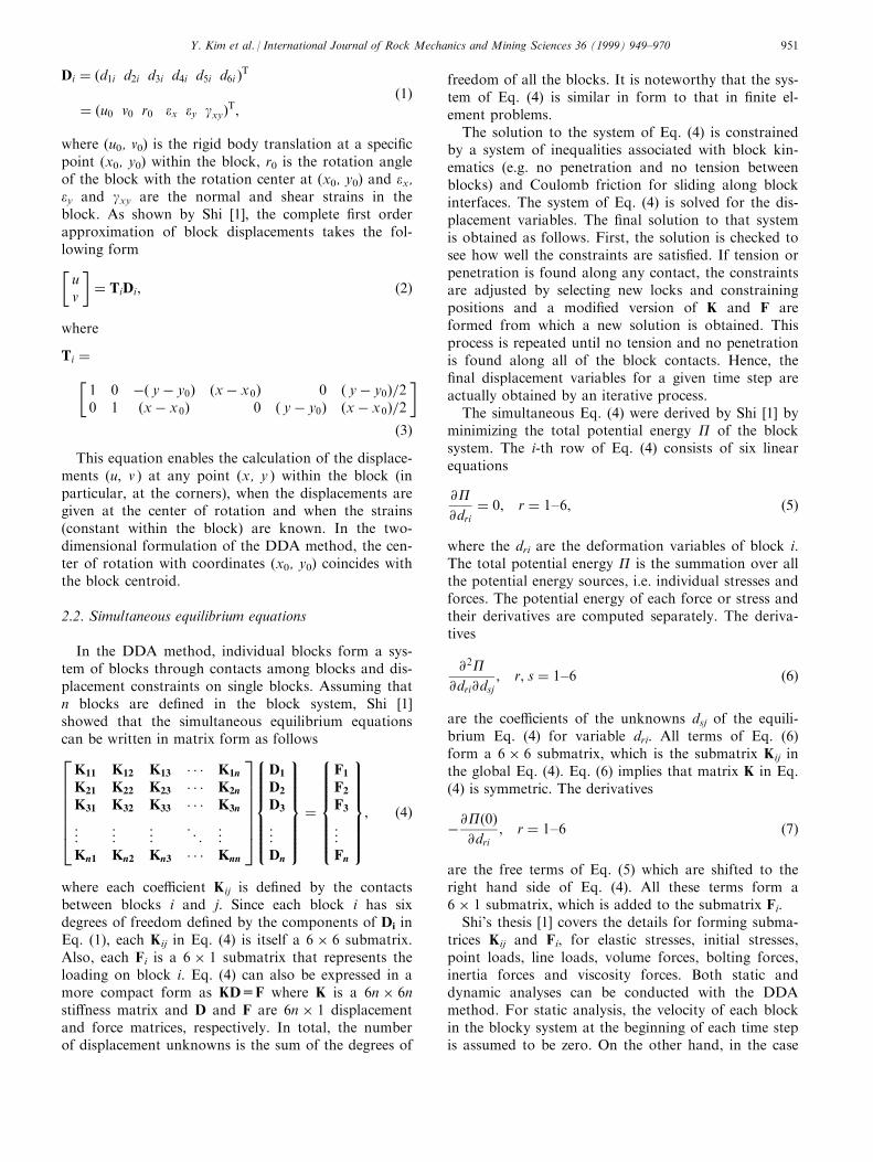
where (u0, v0) is the rigid body translation at a speci®cpoint (x0, y0) within the block, r0 is the rotation angleof the block with the rotation center at (x0, y0) and ex,ey and gxy are the normal and shear strains in theblock. As shown by Shi [1], the complete ®rst orderapproximation of block displacements takes the fol-lowing form�uv

�� TiDi, �2�

where

Ti ��1 0 ÿ� yÿ y0� �xÿ x0� 0 � yÿ y0�=20 1 �xÿ x0� 0 � yÿ y0� �xÿ x0�=2

��3�

This equation enables the calculation of the displace-ments (u, v ) at any point (x, y ) within the block (inparticular, at the corners), when the displacements aregiven at the center of rotation and when the strains(constant within the block) are known. In the two-dimensional formulation of the DDA method, the cen-ter of rotation with coordinates (x0, y0) coincides withthe block centroid.

2.2. Simultaneous equilibrium equations

In the DDA method, individual blocks form a sys-tem of blocks through contacts among blocks and dis-placement constraints on single blocks. Assuming thatn blocks are de®ned in the block system, Shi [1]showed that the simultaneous equilibrium equationscan be written in matrix form as follows26666664

K11 K12 K13 � � � K1n

K21 K22 K23 � � � K2n

K31 K32 K33 � � � K3n

..

. ... ..

. . .. ..

.

Kn1 Kn2 Kn3 � � � Knn

37777775

8>>>>>><>>>>>>:

D1

D2

D3

..

.

Dn

9>>>>>>=>>>>>>;�

8>>>>>><>>>>>>:

F1

F2

F3

..

.

Fn

9>>>>>>=>>>>>>;, �4�

where each coe�cient Kij is de®ned by the contactsbetween blocks i and j. Since each block i has sixdegrees of freedom de®ned by the components of Di inEq. (1), each Kij in Eq. (4) is itself a 6 � 6 submatrix.Also, each Fi is a 6 � 1 submatrix that represents theloading on block i. Eq. (4) can also be expressed in amore compact form as KD=F where K is a 6n � 6nsti�ness matrix and D and F are 6n � 1 displacementand force matrices, respectively. In total, the numberof displacement unknowns is the sum of the degrees of

freedom of all the blocks. It is noteworthy that the sys-tem of Eq. (4) is similar in form to that in ®nite el-ement problems.

The solution to the system of Eq. (4) is constrainedby a system of inequalities associated with block kin-ematics (e.g. no penetration and no tension betweenblocks) and Coulomb friction for sliding along blockinterfaces. The system of Eq. (4) is solved for the dis-placement variables. The ®nal solution to that systemis obtained as follows. First, the solution is checked tosee how well the constraints are satis®ed. If tension orpenetration is found along any contact, the constraintsare adjusted by selecting new locks and constrainingpositions and a modi®ed version of K and F areformed from which a new solution is obtained. Thisprocess is repeated until no tension and no penetrationis found along all of the block contacts. Hence, the®nal displacement variables for a given time step areactually obtained by an iterative process.

The simultaneous Eq. (4) were derived by Shi [1] byminimizing the total potential energy P of the blocksystem. The i-th row of Eq. (4) consists of six linearequations

@P@dri� 0, r � 1±6, �5�

where the dri are the deformation variables of block i.The total potential energy P is the summation over allthe potential energy sources, i.e. individual stresses andforces. The potential energy of each force or stress andtheir derivatives are computed separately. The deriva-tives

@2P@dri@dsj

, r, s � 1±6 �6�

are the coe�cients of the unknowns dsj of the equili-brium Eq. (4) for variable dri. All terms of Eq. (6)form a 6 � 6 submatrix, which is the submatrix Kij inthe global Eq. (4). Eq. (6) implies that matrix K in Eq.(4) is symmetric. The derivatives

ÿ@P�0�@dri

, r � 1±6 �7�

are the free terms of Eq. (5) which are shifted to theright hand side of Eq. (4). All these terms form a6 � 1 submatrix, which is added to the submatrix Fi.

Shi's thesis [1] covers the details for forming subma-trices Kij and Fi, for elastic stresses, initial stresses,point loads, line loads, volume forces, bolting forces,inertia forces and viscosity forces. Both static anddynamic analyses can be conducted with the DDAmethod. For static analysis, the velocity of each blockin the blocky system at the beginning of each time stepis assumed to be zero. On the other hand, in the case

Y. Kim et al. / International Journal of Rock Mechanics and Mining Sciences 36 (1999) 949±970 951

of dynamic analysis, the velocity of the blocky systemin the current time step is an accumulation of the vel-ocities in the previous time steps.

3. Modeling water-block interaction in DDA

A numerical model was developed to study ¯uid¯ow in deformable naturally fractured rock masses.The model considers a two-dimensional intact rockmass dissected by a large number of fractures (joints)with variable aperture, length, and orientation. Fluid¯ow, which occurs when pressure gradients exist, isassumed to be steady, and laminar or turbulentdepending on the values of the Reynolds number andthe relative roughness of the fracture walls [10]. Fluid¯ow and the rock deformation are fully coupled.

Variations in ¯uid pressure and quantity of ¯uid resultin joint deformation. In turn, joint deformationchanges the joint properties, which therefore changesthe ¯uid pressures and the resistance to ¯uid ¯ow.

3.1. Assumptions

The following assumptions were made when imple-menting the hydro-mechanical coupling in the DDAprogram: (a) the ¯uid is incompressible, (b) the intactrock is impervious, and ¯uid ¯ow takes place in thejoint space only; (c) the rock mass contains a ®nitenumber of joints; (d) the intact rock is linearly elastic;and (e) joint displacements are small relative to thejoint dimensions.

In the ¯ow model, the fracture space is idealized asa system of one-dimensional conduits of constant aper-

Fig. 1. Joint modeling. (a) Representative section of closed joint, (b) Idealized section of closed joint, (c) Representative section of open joint, (d)

Idealized section of open joint.


ture using the approach proposed by Asgian [11]. Theapparent aperture, b, of a conduit representing a jointdepends on the contact between the joint surfaces. Thejoint can be classi®ed as closed or open depending onthe contact state. Consider, for instance, a closed jointwith length, L, and unit width representing the inter-face between two contacting prismatic blocks of thick-ness d1 and d2 as shown in Fig. 1(a). Let n be the jointsurface contact porosity (ratio between joint surfaceopen area and total area) of the closed joint which var-ies between 0 and 1. The joint can be idealized as aportion of void (n ) with a uniform aperture, a, and aportion of contacting solid (1ÿn ) with vanishing aper-ture as shown in Fig. 1(b). The apparent aperture, b,

of the closed joint is de®ned as b=a for the portion ofvoid (n ).

A representative section of an open joint withlength, L, and unit width is shown in Fig. 1(c). Thejoint represents the open interface between two pris-matic blocks of thickness d1 and d2 separated by a gapc. The joint can be idealized as one portion of void (n )with aperture, c+a, and another portion of void(1ÿn ) with aperture, c, as shown in Fig. 1(d). Theapparent aperture, b, of the open joint consists of twocomponents with bn=c+a for the portion of void (n )and b1ÿn=c for the other portion of void (1ÿn ).

3.2. Con®guration of water-block interaction model

As shown in Fig. 2, the hydro-mechanical modelconsists of two major components: the DDA methodfor the rock mass and the FEM method for joint ¯ow.The initial properties of the joints such as aperture,length, orientation, and boundary conditions from theDDA program are used to compute the piezometricheads and ¯uid quantities at the joints with a FEMsubroutine called RFLOW. The seepage forces actingon the rock blocks are computed from the piezometricheads using a subroutine called WPRESSURE. In theDDA program, joint deformation is computed usingthe seepage forces. In turn, joint deformation changesthe joint properties such as aperture, length, and orien-tation. A computational loop is followed until the

Fig. 2. Water-block interaction model.

Fig. 3. Compilation of di�erent ¯ow laws and their range of validity for a single fracture. The dashed lines represent mathematical boundaries

by Amadei et al. [12] and the solid lines the boundaries determined experimentally by Louis [10].


results converge according to a criterion selected bythe user.

3.3. Subroutine RFLOW

Louis [10] showed experimentally that the steady¯ow of water in a single fracture of constant aperture,b, and surface roughness can be laminar or turbulentdepending on the values of the Reynolds number,Re=2bu/n, and the relative roughness, k/Dh, where u isthe average velocity, n the kinematic viscosity of water,k the fracture surface roughness, and Dh the hydraulicdiameter of the fracture which is equal to 2b. Louis[10] also proposed di�erent ¯ow laws relating the fric-tion factor f and the Reynolds number Re which applyin di�erent regions of the (Re, k/Dh) space. Fig. 3shows ®ve such regions I±V, their corresponding math-ematical boundaries and the experimental boundariesproposed by Louis [10].

For parallel ¯ow, and as shown by Amadei et al.[12], the mathematical boundary between turbulenthydraulic smooth ¯ow (region II) and turbulent com-pletely rough ¯ow (III) in Fig. 3 can be expressed as

Re � 2:553

�log

�k=Dh

3:7

��8�8�

For non-parallel ¯ow, and as shown by Amadei etal. [12], the mathematical boundary between laminar¯ow (region IV) and turbulent ¯ow (region V) in Fig.3 can be expressed as

Re � 384�1� 8:8�k=Dh�1:5

��log

�k=Dh

1:9

��2�9�

The mathematical boundaries de®ned by Eqs. (8)and (9) are shown as dashed lines in Fig. 3. Thesemathematical boundaries were used in the nonlinearmodel presented below.

According to Bernoulli's theorem for ideal friction-less incompressible ¯uids, the sum of the pressure head,hp=p/gw, elevation head, he=z, and velocity head,hv=u 2/2g, is constant at every point of the ¯uid, e.g.

p

gw

� z� u2

2g� H� hn � constant � Ht �10�

where p is the pressure, z the elevation, u the averagevelocity, H the piezometric head (=hp+he), and Ht

the total head.In the steady ¯ow of water in a single fracture of

constant aperture, b, and length, L, the total head loss,DHt, (also equal to the piezometric head loss, DDH )takes place due to the viscous resistance within thefracture. As shown by Louis [10], the average velocity,u, and the gradient of piezometric head, i=DDH/L,(also equal to the gradient of total head, DDHt/L ) foreach hydraulic region of Fig. 3 can be written as fol-lows

u � Kia � K

�DHL

�a

�11�

where DH is the piezometric head loss. Values of thehydraulic conductivity, K, and the exponent, a, foreach ¯ow region of Fig. 3 are reported in Table 1. Foreach hydraulic region, the element discharge, Q, andthe piezometric gradient, i=DDH/L, are such that

Q � ub � Kb

�DHL

�a

�12�

Equation (12) can be rewritten as

Q � TDH with T � Kb

La DHaÿ1 �13�

where T is the so-called fracture transmissivity.Equation (13) is then modi®ed depending on the

contact state (closed or open) between the joint sur-faces. For a closed joint (Fig. 1(b)), the element dis-charge, Q, is de®ned as

Q � TDH with T � nKb

La DHaÿ1 �14�

For an open joint (Fig. 1(d)), the element discharge,Q, is de®ned as

Q � TDH with

T � nKnbnLan

DH anÿ1 � �1ÿ n�K1ÿnb1ÿnLa1ÿn

DH a1ÿnÿ1, �15�

where Kn and an are respectively the hydraulic conduc-

Table 1

Expression of hydraulic conductivity and degree of nonlinearity for the di�erent hydraulic regions of Fig. 3 (after Louis [10])

Hydraulic region Hydraulic conductivity (K) Exponent (a ) Flow condition

I KI � gb2=12n 1.0 laminar

II KII��1=b��g=0:079��2=n�0:25 � b3�4=7 4/7 turbulent

III KIII � 4��gp

log�3:7=�k=Dh��bp

0.5 turbulent

IV KIV � �gb2�=�12n�1� 8:8�k=Dh�1:5�� 1.0 laminar

V KV � 4��gp

log�1:9=�k=Dh��bp

0.5 turbulent


tivity and exponent for one portion of void (n ) withapparent aperture bn=c+a. Likewise, K1ÿn and a1ÿnare respectively the hydraulic conductivity and expo-nent for the other portion of void (1ÿn ) with apparentaperture b1ÿn=c.

Consider now a single planar joint element, i, oflength L i and constant aperture b i as shown in Fig.4(a). Eq. (13) can be used to compute the dischargethrough the joint element in terms of the piezometrichead loss between its two end nodes de®ned here as jand k. The discharge at node k, Qk

i , and the dischargeat node j, Qj

i, are equal to

Qik � T iDH i � T i

�Hi

k ÿHij

�

Qij � ÿT iDH i � ÿT i

�Hi

k ÿHij

��16�

These two equations can be rewritten in matrix formas follows:

(Qi

k

Qij

)� T i

�1 ÿ1ÿ1 1

�(Hi

k

Hij

)or Qi � TiHi, �17�

where Qi is the element nodal discharge vector, Ti theelement characteristic matrix, and Hi the elementnodal piezometric head vector.

So far, the elements in the network have been con-sidered individually, and expressions giving the dis-charges in terms of the nodal piezometric heads havebeen developed. For a complete joint network, how-ever, the interaction between the di�erent elementsneeds to be taken into account. This implies that theremust exist equilibrium at any given node of the net-work between the discharges of the elements connectedto the node, including any in¯ow or out¯ow at thatnode. Consider a simpli®ed model of a fracture net-work below a dam as shown in Fig. 4(b). The quantityCj is the in¯ow (C1 and C3) or out¯ow (C5 and C7) atany node j. In general, any Cj will be positive forin¯ow (C1 and C3) and negative for out¯ow (C5 andC7). Equilibrium at any node means that the sum ofthe discharges of the elements connected to the nodeequals the in¯ow or out¯ow at that node. For anynode j, the equilibrium equation can be expressed asfollows:X

i

Qij � Cj �18�

where the summation runs over all elements connectedto node j. By repeating the procedure for all n nodes,and using Eqs. (17) and (18), a system of equilibriumequations can be derived e.g.266664T11 T12 . . . T1n

T21 T22 . . . T2n

..

. ... . .

. ...

Tn1 Tn2 . . . Tnn

3777758>>>><>>>>:H1

H2

..

.

Hn

9>>>>=>>>>; �8>>>><>>>>:C1

C2

..

.

Cn

9>>>>=>>>>;or TH � C

�19�

where T is the network characteristic matrix, H is thenetwork piezometric head vector, and C is the network¯ow vector. Before the total system of Eq.(19) can besolved, it is necessary to introduce the boundary con-ditions for the network nodes. The boundary con-ditions at a given node j can be of two types; speci®edpiezometric head (Hj) or speci®ed ¯ow (Cj).

The total system of Eq.(19) is a nonlinear systemdue to the fact that T depends on H. However, it canbe solved by successive iterations. First, for each jointelement, ¯ow is assumed to be laminar with a=1.0and K=KI or KIV and an initial value for the nodalpiezometric head, Hini, is assumed for each node.Thefracture transmissivity, T, is computed using Eqs. (14)or (15) for each joint element, and the total system of

Fig. 4. Construction of total system of equations. (a) Single joint el-

ement, (b) Joint network.


Eq. (19) is formed using Eqs. (17) and (18). The totalsystem of equations is solved by the Gauss eliminationmethod to obtain a new value of the nodal piezometrichead, Hnew, for each node. The velocity, u, de®ned byEq. (11) and the Reynolds number, Re = 2bu/n, arecalculated for each joint element using the new valueof the nodal heads. Using Fig. 3, the values of Re andthe relative roughness, k/Dh, determine if the ¯ow ineach joint element is laminar or turbulent. If the ¯owis laminar, a and K remain the same. If, on the otherhand, turbulent ¯ow develops, new values of a and Kare selected using Fig. 3 and Table 1 for each joint el-ement, and a new initial value for the nodal piezo-metric head is assumed with Hini=Hnew for each node

in the next iteration. Then, using Eqs. (14) or (15), anew fracture transmissivity, T, is computed for each el-ement, and a new total system of equations is formed.The total system of equations is solved to obtain anew value of the nodal piezometric head, Hnew, foreach node. The process is repeated until, for two suc-cessive steps, a and K remain the same and|HnewÿHini|/Hini is below a minimum tolerance speci-®ed by the user.

3.4. Subroutine WPRESSURE

A new algorithm for computing seepage forces act-ing on rock blocks from the nodal piezometric heads

Fig. 5. Conversion of nodal head into point load.


was developed. The ¯uid pressure acting on the rockblocks can be computed from the values of the press-ure heads at those nodes de®ning the blocks. The ¯uidpressures are transformed as point loads along thesides of each rock block. Then, the point loads aregiven as boundary conditions in the discontinuous de-formation analysis. Using this approach, there is noneed to arti®cially regulate the deformations of thejoints as in other methods. Therefore, the rock blockscan deform freely according to block system kin-ematics.

As an example, consider ¯ow through the joint net-work of Fig. 5. Subroutine RFLOW gives value of thepiezometric head, H, at each node. Then, at eachnode, the pressure head, hp, can be computed from H,and the elevation head, he=yÿyd, ashp � Hÿ he � Hÿ y� yd �20�

where y is the vertical coordinate of the node, yd thevertical coordinate of the datum line. For rock block,i, in Fig. 5, hp can be calculated by using Eq. (20) atnodes 1 and 2 with hp1=H1±y1+yd andhp2=H2ÿy2+yd. The pressures at node 1 and 2 arethen equal to p1=hp1gw and p2=hp2gw, respectively.For a closed joint with a contact porosity, n, the totalseepage force, F, acting on the edge between nodes 1and 2 is calculated as

F � n12 �p1 � p2� � L with

L ��x1 ÿ x2�2 � � y1 ÿ y2�2

q�21�

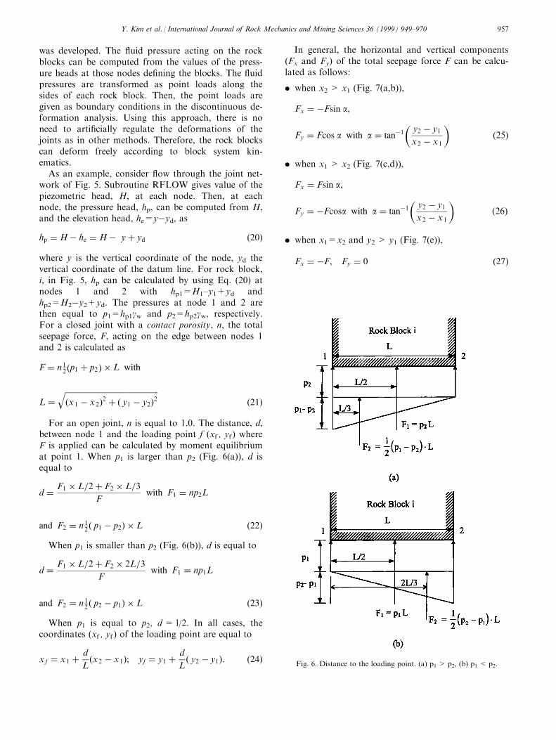
For an open joint, n is equal to 1.0. The distance, d,between node 1 and the loading point f (xf , yf ) whereF is applied can be calculated by moment equilibriumat point 1. When p1 is larger than p2 (Fig. 6(a)), d isequal to

d � F1 � L=2� F2 � L=3

Fwith F1 � np2L

and F2 � n12� p1 ÿ p2� � L �22�

When p1 is smaller than p2 (Fig. 6(b)), d is equal to

d � F1 � L=2� F2 � 2L=3

Fwith F1 � np1L

and F2 � n12� p2 ÿ p1� � L �23�

When p1 is equal to p2, d = l/2. In all cases, thecoordinates (xf , yf ) of the loading point are equal to

xf � x1 � d

L�x2 ÿ x1�; yf � y1 � d

L� y2 ÿ y1�: �24�

In general, the horizontal and vertical components(Fx and Fy) of the total seepage force F can be calcu-lated as follows:

. when x2 > x1 (Fig. 7(a,b)),

Fx � ÿFsin a,

Fy � Fcos a with a � tanÿ1�y2 ÿ y1x2 ÿ x1

��25�

. when x1 > x2 (Fig. 7(c,d)),

Fx � Fsin a,

Fy � ÿFcosa with a � tanÿ1�y2 ÿ y1x2 ÿ x1

��26�

. when x1=x2 and y2 > y1 (Fig. 7(e)),

Fx � ÿF, Fy � 0 �27�

Fig. 6. Distance to the loading point. (a) p1 > p2, (b) p1 < p2.


. when x1=x2 and y1 > y2 (Fig. 7(f)),

Fx � F, Fy � 0 �28�

3.5. Application of seepage forces on rock blocks

Shi [1] derived a formulation for the components ofsubmatrices Fi for the case of point loading. A seepageforce can be considered as a point load acting alongthe edge of a rock block. The seepage force with com-ponents (Fx, Fy ) acts at point (xf , yf ) on rock block, i,

as shown in Fig. 7(a,f). According to Eq. (2), the dis-placement components (uf , vf ) at point (xf , yf ) alongthe edge of rock block, i, are equal to

�ufvf

�� TiDi �

�t11 t12 t13 t14 t15 t16t21 t22 t23 t24 t25 t26

�8>>>>>><>>>>>>:

d1id2id3id4id5id6i

9>>>>>>=>>>>>>;�29�

Fig. 7. Computation of Fx and Fy. (a) x1 < x2, y1ry2, (b) x1 < x2, y1 < y2, (c) x1 > x2, y1 < y2, (d) x1 > x2, y1ry2, (e) x1=x2, y1 < y2, (f)

x1=x2, y1 > y2.


The potential energy associated with the seepageforce with components (Fx, Fy) is then equal to

Pf � ÿÿFxuf � Fyvf

� � ÿÿ uf vf��Fx

Fy

�

Pf � ÿDTi TT

i

�Fx

Fy

� �30�

To minimize Pf , derivatives are computed and yield

fr � ÿ@Pf�0�@dri

� @

@driDT

i TTi

�Fx

Fy

�� Fxt1r � Fyt2r,

r � 1±6

�31�

where fr (r = 1±6,) are the components of a 6 � 1 sub-matrix

TTi

�Fx

Fy

��

0BBBBBB@t11 t21t12 t22t13 t23t14 t24t15 t25t16 t26

1CCCCCCA�Fx

Fy

�4Fi �32�

which is the product matrix of a 6 � 2 matrix (whosecomponents are de®ned in Eq. (3)) and a 2 � 1 matrix.The resulting 6 � 1 submatrix is added to the subma-trix Fi in the global system of Eq. (4).

3.6. Comparison with the experimental work ofGrenoble [13]

As a validity check of the RFLOW subroutine, acomparison was made with the experimental workreported by Grenoble [13], who constructed a physicallaboratory model to simulate two-dimensional ¯owthrough a jointed rock mass. The joint network of themodel was formed by sawing 12.7 mm (0.5 inch) deepand 0.508 mm (0.02 inch) wide slots in the face of a25.4 mm (1.0 inch) thick sheet of Plexiglas. A sche-matic of the complete test set-up is illustrated in Fig.8(a) and the model joint pattern is shown in Fig. 8(b).The water pressure was measured at 24 joint intersec-tion ports as shown in Fig. 8(b). Grenoble [13] con-ducted nine tests (T1-3 to T1-11) subjecting the modelto hydraulic gradients ranging between 0.01 and 2.84(resulting in a head di�erential across the model ran-ging between 0.762 cm and 172.84 cm). The test pro-cedure consisted of applying a head di�erential,allowing the system to come to equilibrium, and thenreading the head values at the measurement ports.

As the laboratory model was made of one plate withslots, all blocks in the DDA model were modeled assubblocks. The Plexiglas was assumed to have a unitweight of 11.7 kN/m3, a Young's Modulus of 3.1 GPaand a Poisson's ratio of 0.35. The joints were assumed

to have no friction or cohesion. The kinematic vis-cosity of water was taken equal to 1.005 � 10ÿ6 m2/sec. Six representative tests (T1-5 to T1-10) were ana-lyzed by the DDA program containing the RFLOWsubroutine (Table 2). For each test, the head valuescomputed by the revised DDA program were com-pared with the values measured in the laboratorymodel at all measurement ports (Table 2). The error inhead value, Ei, at each measurement port, i, was calcu-lated as follows

Ei � hl ÿ hd

Hÿ h, �33�

where hl is the head value measured in the laboratory;hd is the value predicted by the DDA program; H isthe upstream head; and h is the downstream head. Foreach test, the average error in head value, Eh, for eachtest was calculated as

Eh � 1

n

Xni�1jEij, �34�

where n (n = 24) is the number of measurement ports.Values of Eh are reported in Table 2.

The results in Table 2 indicate that the average errordoes not exceed 5.83% and its magnitude increaseswith the hydraulic gradient. This increase is probablydue to the fact that the pressure ports disturb the ¯owand the magnitude of the disturbance increases withthe ¯ow velocity [13].

3.7. Comparison with the analytical solution of Sneddonand Lowengrub [14]

As a validity check of the WPRESSURE subroutinein the DDA program, the problem of the opening of acrack (joint) in an in®nite domain subjected to an in-ternal pressure was considered. The geometry of theproblem is shown in Fig. 9(a). An internal pressure Pis applied on the walls of a crack of length, 2L, result-ing in a maximum deformation, Dn,max, at the centerof the crack.

Two DDA models for this problem are shown inFig. 9(b,c). The crack length is 2L = 20 m and thedomain of analysis is 10L � 10L (100 m � 100 m). Thecrack has a friction angle of 458, and no cohesion. Theintact rock has a unit weight of 26.0 kN/m3, aYoung's modulus of 2.5 GPa, and a Poisson's ratio of0.25. The ¯uid has a kinematic viscosity of 2.0 � 10ÿ7

m2/sec. At the crack ends (x=2L ), the pressureheads were ®xed at 22.45 m as boundary conditions,thus a constant ¯uid pressure of 0.22 MPa was appliedon the crack wall surfaces. Two cases were consideredfor comparison in which the walls of the crack were


divided into 6 subblocks (Fig. 9(b)) and 10 subblocks(Fig. 9(c)).

The crack opening for this problem was also com-puted using the analytical solution given by Sneddonand Lowengrub [14]:

Dn � 2�1ÿ n�G

PL

��ÿ1ÿ x2=L2

�q, �35�

where L is the crack half-length, Dn the crack openingalong the interval ÿL R x R L, G is the shear mod-ulus of the elastic medium; P is the pressure acting onthe crack wall surfaces; x is the distance along thecrack measured from the center of the crack; and n isthe Poisson's ratio.

The analytical and numerical predictions for thecrack wall deformation pro®les for the two cases arecompared in Figs. 10(a) and 10(b). At the center of thecrack, the numerical solution deviates from the analyti-cal solution by 3.9% for the case in which 6 subblocksare used to compute the crack displacement (Fig.10(a)). When 10 subblocks are used instead (Fig.10(b)), the deviation of the numerical solution fromthe analytical solution reduces to 1.1%. At the crackends (x=2L ), the numerical solution deviates fromthe analytical solution by 15.8% for the 6 subblockscase and 14.5% for the 10 subblocks case. At the endsof the idealized crack, the crack opening is zero, yetthe gradient of the opening is in®nite. This large devi-ation at the crack ends results because the discretiza-

Fig. 8. Laboratory model of Grenoble [13]. (a) Schematic of the complete laboratory test set-up, (b) Layout of the joint pattern in the physical

model.


tion of the crack is too coarse to account for the sharpcurvature of the crack at its ends. Except for the crackends, Fig. 10(a,b) indicate good agreement between thenumerical and analytical predictions.

3.8. E�ect of water level on tunnel stability

The excavation of a (half) circular tunnel is con-sidered as a numerical example. The tunnel has a di-ameter, D, of 10 m and is located at a depth of 409.6m below the surface. The water level varies between100 and 500 m above the center of the tunnel. Thedomain of analysis is 5D (50 m) wide and 4D plus tun-nel height (46.71 m) high. A vertical compressive stressof 10 MPa is applied on the top boundary of thedomain (to simulate the load associated with 384.6 mof rock) and no lateral deformation is allowed. Theintact rock has a unit weight of 26 KN/m3, a Young'smodulus of 3.6 GPa, and a Poisson's ratio of 0.2. The

joints have a spacing of 4 m, a friction angle of 358,and a cohesion of 0.5 MPa. No reinforcement isapplied in this example. As boundary conditions, onlyelevation heads (zero pressure heads) were applied onthe nodes along the excavated surface of the tunnel.

Without water the settlement of the tunnel roof wasfound to be equal to 165.2 mm (Table 3). The tunnelroof deforms but does not collapse as shown in Fig.11(a). As the water level increases, the tunnel roofsettlement increases resulting in complete collapse ofthe tunnel (see Table 3 and Fig. 11(b±f)).

4. Modeling sequential loading or unloading

4.1. Sequential excavation algorithm

A new algorithm to simulate sequential loading orunloading has been developed and implemented into

Table 2

Average error of the DDA program compared with experimental results by Grenoble [13]

Test No. T1-5 T1-6 T1-7 T1-8 T1-9 T1-10

H (cm) 80.52 97.28 115.7 134.37 151.38 227.2

h (cm) 71.76 71.37 71.37 71.37 72.01 54.36

Dh (cm) 8.76 25.91 44.33 63 79.37 172.84

L (cm) 60.96 60.96 60.96 60.96 60.96 60.96

i(Dh/L) 0.14 0.42 0.73 1.03 1.30 2.84

Method DDA Lab Error DDA Lab Error DDA Lab Error DDA Lab Error DDA Lab Error DDA Lab Error

Port hd (cm) hl (cm) Ei (%) hd (cm) hl (cm) Ei (%) hd (cm) hl (cm) Ei (%) hd (cm) hl (cm) Ei (%) hd (cm) hl (cm) Ei (%) hd (cm) hl (cm) Ei (%)

1 79.93 79.88 ÿ0.58 95.55 95.38 ÿ0.69 112.60 112.65 0.11 130.18 130.56 0.60 146.35 147.45 1.38 215.75 217.81 1.19

2 79.96 79.88 ÿ0.87 95.61 95.50 ÿ0.39 112.70 113.16 1.03 130.28 131.19 1.45 146.30 147.70 1.76 216.00 218.57 1.48

3 79.17 79.25 0.87 93.27 93.47 0.78 108.71 109.22 1.15 124.64 126.37 2.74 139.01 142.49 4.38 200.18 201.93 1.01

4 80.01 79.88 ÿ1.45 95.76 95.50 ÿ0.98 112.90 112.52 ÿ0.86 130.63 130.56 ÿ0.12 146.61 146.94 0.42 216.89 217.04 0.09

5 80.04 80.01 ÿ0.29 95.86 95.89 0.10 113.08 113.54 1.03 130.94 131.32 0.60 146.94 148.08 1.44 217.68 218.06 0.22

6 80.37 80.26 ÿ1.16 96.82 96.77 ÿ0.20 114.91 114.68 ÿ0.52 133.22 133.10 ÿ0.20 149.91 150.11 0.26 224.08 224.03 ÿ0.037 78.84 78.99 1.74 92.30 92.84 2.06 107.11 108.20 2.46 122.22 124.84 4.15 136.42 140.97 5.73 194.06 200.79 3.89

8 78.89 78.99 1.16 92.46 92.96 1.96 107.32 108.46 2.58 122.61 125.10 3.95 136.86 141.35 5.66 195.07 201.17 3.53

9 75.64 74.80 ÿ9.57 82.88 83.06 0.69 90.93 91.19 0.57 99.36 102.11 4.35 107.52 114.81 9.18 131.60 141.61 5.79

10 75.36 75.31 ÿ0.58 82.02 81.92 ÿ0.39 89.66 89.41 ÿ0.57 97.31 98.55 1.98 105.31 111.00 7.17 125.98 133.86 4.56

11 75.97 75.95 ÿ0.29 83.82 83.82 0.00 92.58 91.82 ÿ1.72 101.68 103.51 2.90 110.49 116.33 7.36 138.00 144.40 3.70

12 76.73 76.96 2.61 86.13 87.00 3.33 96.70 97.79 2.46 107.26 111.38 6.53 117.45 125.60 10.27 153.09 165.10 6.95

13 76.86 76.96 1.16 86.46 87.38 3.53 97.31 98.68 3.09 108.08 112.40 6.85 118.41 127.00 10.82 155.17 167.39 7.07

14 76.40 76.45 0.58 85.12 85.60 1.86 94.87 95.63 1.72 104.78 107.32 4.03 114.20 120.90 8.45 146.53 157.99 6.63

15 76.61 76.58 ÿ0.29 85.73 86.23 1.96 96.01 96.52 1.15 106.27 109.73 5.48 116.18 123.44 9.15 150.83 163.20 7.16

16 76.81 76.71 ÿ1.16 86.39 86.61 0.88 97.03 97.28 0.57 107.80 110.36 4.07 118.57 123.95 6.78 154.41 163.96 5.53

17 73.05 72.77 ÿ3.19 75.21 75.18 ÿ0.10 77.90 77.72 ÿ0.40 80.67 82.30 2.58 84.02 89.41 6.78 79.83 86.49 3.85

18 72.75 72.39 ÿ4.06 74.30 74.42 0.49 76.53 76.45 ÿ0.17 78.49 78.99 0.81 81.33 85.09 4.74 73.79 77.98 2.42

19 73.71 73.53 ÿ2.03 77.17 77.47 1.18 81.23 81.79 1.26 85.42 88.65 5.12 90.22 96.14 7.46 92.91 100.46 4.36

20 73.13 72.90 ÿ2.61 75.41 75.82 1.57 78.44 78.74 0.69 81.18 83.31 3.39 84.91 90.68 7.26 81.15 89.66 4.92

21 74.27 74.04 ÿ2.61 78.82 78.99 0.69 83.97 84.33 0.80 89.43 92.96 5.60 95.30 100.46 6.50 103.99 113.67 5.60

22 72.85 72.52 ÿ3.77 74.60 74.68 0.29 76.96 77.34 0.86 79.20 83.06 6.13 81.99 87.63 7.10 75.69 87.76 6.98

23 72.57 72.26 ÿ3.48 73.74 73.91 0.69 75.39 75.82 0.97 77.11 79.50 3.79 79.35 83.82 5.63 70.05 78.11 4.66

24 72.29 71.88 ÿ4.64 72.95 72.64 ÿ1.18 74.14 74.17 0.06 75.21 77.09 2.98 76.99 80.39 4.29 64.82 71.63 3.94

Eh (%) 2.11 1.08 1.12 3.35 5.83 3.98


the DDA program. The algorithm can be used, forinstance, to model the di�erent phases of undergroundexcavation. The algorithm consists of an iterative pro-cedure where in situ stresses are ®rst computed in allrock blocks before excavation. Then, the new stressdistribution is determined following the ®rst excavationstep. The new stresses are then taken as initial stressesfor the next excavation step. This iterative procedurecontinues until the end of the excavation process.

4.2. Analysis of excavation sequence of tunnels

As an example of application of the method, a rockmass 30 m wide and 20 m high consisting of 17 rock

blocks is considered (Fig. 12). Three point loads areapplied on block #15, to simulate structural loads atthe ground surface. The intact rock has a unit weightof 23.6 kN/m3, a Young's Modulus of 48 GPa, and aPoisson's ratio of 0.3. The joints have a friction angleof 408 and a cohesion of 4.0 MPa. No water ¯ow wasconsidered. Two sequences of excavation of a horse-shoe tunnel in the rock mass of Fig. 12 were con-sidered and are referred to as top-to-bottom andbottom-to-top. In the top-to-bottom (ex-t) excavationsequence, ®ve blocks (numbered #32, #33, #31, #30,#29 in Fig. 12) were removed sequentially as shown inFig. 13(b±f). In the bottom-to-top (ex-b) excavationsequence, ®ve di�erent blocks (numbered #29, #30,#31, #32, #33) were removed sequentially as shown inFig. 14(b±f). The major principal stress s1 in blocks#18, #19, #23, #22 and #20 located on the left of theexcavation surface was calculated for both excavationsequences. The results are plotted in Fig. 15(a,b,c,d,e).

Figure 15(a±e) indicate that the top-to-bottom exca-vation sequence induces much less stress concentrationin the rock blocks adjacent to the excavated rock sur-face than the bottom-to-top excavation sequence. Theresults also show that in the bottom-to-top excavationsequence, the stress increases rapidly, which is morecritical for the stability of the ®nal excavated rock sur-

Fig. 9. Analysis of a pressurized crack in an in®nite domain. (a) Representative section of a crack, (b) DDA model with crack walls divided into

6 subblocks, (c) DDA model with crack walls divided into 10 subblocks.

Table 3

E�ect of water level on the stability of the tunnel in Fig. 11

Water level (m) Roof settlement (mm)

0 165.2

100 237.6

200 706.4

300 1632.8

400 2088.2

500 4514.0


face. At the ®nal excavation step (step 5), the top-to-bottom excavation sequence shows slightly smallerstresses than the bottom-to-top excavation sequence.These results indicate that the ®nal stress distributionis in¯uenced by the stress history induced by the exca-vation. This stress-path dependency is associated withgeometrical nonlinearities in the DDA method asenergy losses take place by friction along the jointsand relative deformation of the blocks.

5. Modeling reinforcement by shotcrete and rockbolts

5.1. Shotcrete and concrete lining algorithm

A new algorithm to model shotcrete or concrete lin-ing has been developed and implemented into theDDA program. The algorithm can be used to modelthe functions of shotcrete or concrete lining, i.e. sealing

of rock surfaces, preserving inherent ground strength,and providing a structural arch. The algorithm creates

shotcrete or concrete lining elements along the exca-vated rock surface with speci®ed thickness and ma-

terial properties, in order to simulate the applicationof shotcrete or the installation of concrete lining onalready reinforced and excavated rock surfaces. After

tunnel excavation, the geometrical data of the rockblocks along the excavated rock surface such as block

numbers and nodal coordinates from the DDA pro-gram are used to compute block numbers and nodalcoordinates of the shotcrete elements. The shotcrete el-

ements are modeled as subblocks with speci®ed thick-ness and material properties. The algorithm adds the

shotcrete elements to existing rock blocks, thus chan-ging the sti�ness matrix of the blocky system. The in-

itial stress in the shotcrete is assumed to be zero. Asthe rock blocks deform, the shotcrete elements arestressed. The new algorithm allows shotcrete elements

Fig. 10. Comparison between analytical and numerical solutions. (a) Case of 6 subblocks, (b) Case of 10 subblocks.


to be installed step-by-step and therefore to simulatethe construction sequence. In that case, the stresses inthe shotcrete elements in a previous step are used asinitial stresses for the next step, whereas the stresses inthe newly installed shotcrete elements are assumed tobe zero.

5.2. Rockbolt algorithm

The rockbolt algorithm suggested by Shi [1] wasmodi®ed to be applicable to the case of sequential ex-cavation and reinforcement, in which the axial force ofa rockbolt at a previous step is applied as preloadingin the next step. The algorithm applies a spring withspeci®ed sti�ness between the starting and endingpoints of the rockbolt, thus changing the sti�nessmatrix of the blocky system. Consider a rockbolt con-necting point P1 (x1, y1) of block 1 and point P2 (x2,y2) of block 2, which are not necessarily the vertices ofthe blocks as shown in Fig. 16(a). The length of therockbolt is

l ��x1 ÿ x2�2 � � y1 ÿ y2�2

q�36�

The preloading of the rockbolt is assumed to bezero. As the rock blocks move as shown in Fig. 16(b),the rockbolt extends by an amount Dl equal to

Fig. 11. E�ect of water level on tunnel stability. (a) No water, (b)

W.L.: 100 m, (c) W.L.: 200 m, (d) W.L.: 300 m, (e) W.L.: 400 m, (f)

W.L.: 500 m.

Fig. 12. Initial con®guration for the analysis of sequential excavation

of a tunnel.

Fig. 13. Stress distribution for top-to-bottom excavation sequence.

(a) Initial state (step 0), (b) step 1, (c) step 2, (d) step 3, (e) step 4, (f)

step 5.


Dl ��Di �T�Ti �T

�lxly

�ÿ �Dj

�T�Tj

�T� lxly

��, �37�

where

lx � 1

l�x1 ÿ x2� ly � 1

l� y1 ÿ y2� �38�

are the direction cosines of the rockbolt. If s is thesti�ness of the rockbolt, the axial force in the rockboltis

F � ÿsDll

�39�

The axial force in the rockbolt at a previous step isapplied to the rockbolt as preloading in the next stepas shown in Fig. 16(c).

The components Fx and Fy of the preloading forceat point P1 '(x1 ',y1 ') in block 1 are equal to

Fx � ÿF lx and Fy � ÿF ly �40�Likewise, the components Fx and Fy of the preload-

ing force at point P2 '(x2 ',y2 ') in block 2 are equal to

Fx � F lx and Fy � F ly �41�The preloading force at each point can be con-

sidered as point loading. For each block, the 6 � 1

submatrix for point loading is computed using Eqs.(29±32) and is added to the submatrix Fi in the globalsystem of Eq. (4).

5.3. E�ect of reinforcement on tunnel stability

The excavation and reinforcement by rockbolt of a(half) circular tunnel is considered as an example ofapplication of the method. The tunnel has a diameter,D, of 10 m and is located at a depth of 409.6 m belowthe surface. The water level is 400 m above the centerof the tunnel. The domain of analysis is 5D (50 m)wide and 4D plus tunnel height (46.71 m) high. A ver-tical compressive stress of 10 MPa is applied on thetop boundary of the domain (to simulate the load as-sociated with 384.6 m of rock) and no lateral defor-mation is allowed. The intact rock has a unit weight of26 KN/m3, a Young's modulus of 3.6 GPa, and aPoisson's ratio of 0.2. The joints have a spacing of 4m, a friction angle of 358, and a cohesion of 0.5 MPa.After excavation of the tunnel, two rockbolts (unten-sioned end-bearing type) were installed across the twovertical joints intersecting the tunnel roof. The sti�nessof the rockbolts varies between 0 and 1 � 1012 N/m.

Without rockbolt reinforcement, the tunnel roof col-lapses as shown in Fig. 17(a) and the settlement of the

Fig. 14. Stress distribution for bottom-to-top excavation sequence. (a) Initial state (step 0), (b) step 1, (c) step 2, (d) step 3, (e) step 4, (f) step 5.


tunnel roof was found to be equal to 1632.8 mm(Table 4). As the sti�ness of the rockbolts increases,the tunnel roof settlement decreases (see Table 4 andFig. 17(b,c,d,e,f)). Also, Table 4 indicates that theaxial force in the rockbolts increases with the sti�nessof the rockbolts.

6. Case study: modeling the excavation andreinforcement of the Unju tunnel

The Unju tunnel was selected as a case study(Daewoo Institute of Construction Technology [15]).

The tunnel is located in Yeongigun

Chungchungnamdo (Korea) and is part of the

``Kyungbu High Speed Railway Project''. Its depth

ranges between 0 and 277.6 m (109K 820) and has a

length of 4.02 km. A tunnel section (Station 109K 440)

was selected for numerical analysis using our DDA

program.

The half circular tunnel was excavated by the single

bench cut method, and reinforced by shotcrete (thick-

ness of 10 cm), rockbolts (diameter of 25 mm and

length of 4 m) and concrete lining (thickness of 0.4 m).

Rockbolts (untensioned end-bearing type) were

installed along the upper half surface of the tunnel

Fig. 15. Variation of s1 with step of excavation for the two excavation sequences of Figs. 13 and 14. (a) block #18, (b) block #19, (c) block #23,

(d) block #22, (e) block #20.


only. The spacing of the rockbolts was 2 m longitudin-ally and 11.38 latitudinally (with a total number of 15).The ground condition above the tunnel is representedin Fig. 18. The radius of the excavation is 7.6 m (tun-nel radius=7.1 m, shotcrete thickness=0.1 m, liningthickness=0.4 m). The geology of the station consistsof augen and banded gneiss. From the geological siteinvestigation report, the ground above the tunnel ismostly hard rock with a very small depth of weatheredrock and soft rock. The intact rock has a unit weightof 26 kN/m3, a Young's modulus of 3.6 GPa, and aPoisson's ratio of 0.2. The joints have a friction angleof 33.58 and a cohesion of 0.11 MPa. The shotcretehas a unit weight of 23 kN/m3, a Young's modulus of

15 GPa, and a Poisson's ratio of 0.25. The Young'smodulus of the rockbolts is 214 GPa. The domain ofanalysis was set as 5D horizontally and 4D (plus tun-nel height) vertically, where D is the tunnel diameterequal to 15.2 m. A vertical compressive stress of 4.83MPa was applied on the top boundary of the domain(to simulate the load associated with 185.7 m of rock).

The joint location and orientation data for station109K 440 used in the DDA analysis were obtained

Fig. 16. Computation of rockbolt preloading. (a) Initial state, (b)

Deformed state, (c) Conversion of axial force of rockbolt as preload-

ing in next step.

Fig. 17. E�ect of rockbolt on tunnel stability for di�erent values of

rockbolt sti�ness. (a) No rockbolt, (b) sti�ness: 1 � 106 N/m, (c)

sti�ness: 1 � 107 N/m, (d) sti�ness: 1 � 109 N/m, (e) sti�ness:

1 � 1011 N/m, (f) sti�ness: 1 � 1012 N/m.

Table 4

E�ect of rockbolt sti�ness on the stability of the tunnel in Fig. 17

Rockbolt Sti�ness (N/m) Rockbolt Axial force (N ) Roof settlement (mm) Rockbolt reinforcement

0 0 1632.8 no

1 � 106 2.29 � 105 1204.1 yes

1 � 107 1.61 � 106 871.9 yes

1 � 109 3.39 � 107 286.6 yes

1 � 1011 7.91 � 108 108.8 yes

1 � 1012 1.20 � 109 69.3 yes


from tunnel face mapping photographs at Station109K 442 located near the station of interest. Thejoints were assumed to be continuous and to extendover the entire domain of analysis. The initial geome-try is shown in Fig. 19(a). Construction (excavationand reinforcement) of the tunnel was conducted in ®vesteps outlined in Table 5. These ®ve steps were simu-lated using our DDA program. The stress distributionat the end of each step is shown in Fig. 19(b±f).

The tunnel roof settlement, the axial force in the 15rockbolts, and the tangential stresses in the shotcretesegments were predicted using the DDA analysis andcompared with actual ®eld measurements. The com-puted and measured data are listed in Table 6. Theseresults indicate that rockbolts #7 and #10, which inter-sect natural rock joints, develop large tensile forces (42and 81 kN). This observation shows the e�ectivenessof rockbolt reinforcement in preventing relative move-ment between blocks in a rock mass. The stresses inthe shotcrete show small compression. The results inTable 6 indicate that rockbolts act as a major re-inforcement of rock blocks and shotcrete functions asauxiliary reinforcement such as sealing of rock surface,preserving inherent ground strength and providing astructural arch.

7. Conclusion

Three major extensions were implemented into theoriginal DDA program of Shi [1] and modi®ed by Lin[8]. The extensions include hydro-mechanical couplingbetween rock blocks and water ¯ow in fractures,sequential loading and unloading, and rock reinforce-ment by shotcrete, rockbolt and concrete lining.

The hydro-mechanical coupling algorithm is veryimportant in rock engineering problems where seepagetakes place in natural fractures and joints. Seepage

forces and water pressure can be controlling factors inrock mass stability as illustrated in the tunnel examplepresented in this paper. The new algorithm is limitedto two-dimensional steady state ¯ow and needs to bemodi®ed to include transient ¯ow phenomena.

Fig. 18. Ground condition of the Unju tunnel (station 109K 440).

Fig. 19. Construction sequence of the Unju tunnel (109K 440). (a)

Step 0, (b) step 1, (c) step 2, (d) step 3, (e) step 4, (f) step 5.


The sequential loading (or unloading) algorithmallows for changes in loading conditions that canoccur in rock engineering problems. In the examplespresented herein, the changes were associated with theexcavation of underground openings. The same algor-ithm could also be used to model surface excavationsassociated with road cuts, open pit mining, quarrying,etc. It is likely that the overall ®nal stability of a rockmass depends on the excavation sequence and the cor-responding stress history. This interesting phenomenoncan now be studied and researched using our newDDA program.

The shotcrete or concrete lining algorithm createsshotcrete or concrete lining elements along the exca-

vated rock surface with speci®ed thickness and ma-terial properties, which simulates applying shotcrete orinstalling concrete lining on already reinforced andexcavated rock surfaces. The rockbolt algorithmsuggested by Shi [1] was modi®ed to be applicable tothe cases of sequential excavation and reinforcement,in which axial forces of rockbolts at a previous stepare applied to the rockbolts as preloading in the nextstep.

The DDA program with the three new extensionscan now be used as a practical tool in the design ofunderground structures such as tunnels or caverns. Itcan also be used to analyze the stability of concretedams on fractured rock masses. The main contribution

Table 5

Steps of excavation and reinforcement for the Unju tunnel

Step Contents

0 Initial state without excavation

1 Excavation of upper half section

2 Reinforcement of the upper half section with shotcrete and rockbolts

3 Excavation of lower half section

4 Reinforcement of lower half section with shotcrete

5 Reinforcement of full section with concrete lining

Table 6

Comparison between computed and measured data (Unju tunnel)

Item DDA Measured data App.

Roof settlement (mm) 4.3 4 +: Down, ÿ: Up

Rock bolt axial force (kN) ÿ3.97 (1) ÿ3.88 (1) ÿ: Compression, +: Extension

ÿ0.70 (2)

4.82 (3)

3.03 (4)

ÿ0.85 (5)

0.93 (6)

41.98 (7)

ÿ0.51 (8) ÿ0.20 (8)

9.68 (9)

80.74 (10)

6.07 (11)

7.01 (12)

ÿ4.86 (13)

ÿ4.58 (14) ÿ4.08 (14)

2.87 (15)

Tangential shotcrete stress (MPa) ÿ0.007 (a)

ÿ0.013 (b) ÿ0.014 (b)

ÿ0.015 (c)

ÿ0.015 (d)

ÿ0.013 (e) ÿ0.012 (e)

ÿ0.035 (f)

ÿ0.035 (g)

ÿ0.036 (h)

ÿ0.026 (i)

ÿ0.009 (j) ÿ0.011 (j)


of this paper is that phases of construction (exca-vation, reinforcement) can now be simulated in a morerealistic way. It is noteworthy that the method pre-sented in this paper is limited to solving two-dimen-sional problems.

Acknowledgements

The support of Daewoo Corporation (ConstructionDivision) is gratefully acknowledged.

References

[1] Shi GH. Discontinuous deformation analysis: a new numerical

model for the statics and dynamics of block systems. Ph.D. the-

sis, University of California, Berkeley, CA, 1988.

[2] Shi GH, Goodman RE. Generalization of two-dimensional dis-

continuous deformation analysis for forward modeling.

International Journal for Numerical and Analytical Methods in

Geomechanics 1989;13:359±80.

[3] Shi GH. Forward and backward discontinuous deformation

analyses of rock systems. In: Proceedings of International

Conference of Rock Joints. Norway: Leon, 1990. p. 731±43.

[4] Ke TC, Goodman RE. Discontinuous deformation analysis and

`the arti®cial joint concept'. In: Proceedings of 1st NARMS,

UT, Austin, 1994. p. 599±606.

[5] Yeung MR, Klein SJ. Application of the discontinuous defor-

mation analysis to the evaluation of rock reinforcement for tun-

nel stabilization. In: Proceedings of 1st NARMS, UT, Austin,

1994. p. 607±14.

[6] Salami MR, Banks D. Discontinuous deformation analysis

(DDA) and simulations of discontinuous media. In: Proc. of the

First International Forum on Discontinuous Deformation

Analysis (DDA) and Simulations of Discontinuous Media,

Berkeley, CA, 1996.

[7] Ohnishi Y. Proc. of the Second International Conference on

Analysis of Discontinuous Deformation, Kyoto, Japan, 1997.

[8] Lin CT. Extensions to the discontinuous deformation analysis

for jointed rock masses and other block systems. Ph.D. thesis,

University of Colorado at Boulder, CO, 1995.

[9] Szechy K. The Art of Tunnelling. Budapest: Akademiai Kiado,

1967.

[10] Louis C. A study of groundwater ¯ow in jointed rock and its

in¯uence on the stability of rock masses. Imperial College,

Rock Mechanics Research Report No. 10, 1969.

[11] Asgian MI. A numerical study of ¯uid ¯ow in deformable,

naturally fractured reservoirs. Ph.D. thesis, University of

Minnesota, MN, 1988.

[12] Amadei B, Carlier JF, Illangasekare TH. E�ects of turbulence

on fracture ¯ow and advective transport of solutes. Int J Rock

Mech Min Sci Geomech Abs 1995;32:343±56.

[13] Grenoble BA. In¯uence of geology on seepage and uplift in

concrete gravity dam foundations. Ph.D. thesis, University of

Colorado at Boulder, CO, 1989.

[14] Sneddon IN, Lowengrub M. Crack problems in the classical

theory of elasticity. New York: John Wiley and Sons, Inc, 1969.

[15] Daewoo Institute of Construction Technology. Final report on

instrumentation of UNJU tunnel ± Kyungbu High Speed Rail

Way Project 4-3 Section. Suwon, Korea: Deawoo Co.

(Construction Division), 1995.


Modeling the e•ect of water, excavation sequence and rock...

Documents

Transcript of Modeling the e•ect of water, excavation sequence and rock...