MODELING TERM STRUCTURE DYNAMICS: AN INFINITE …rama/papers/IJTAF.pdf · Modeling Term Structure...

May 3, 2005 14:10 WSPC-104-IJTAF SPI-J071 00304

International Journal of Theoretical and Applied FinanceVol. 8, No. 3 (2005) 357–380c© World Scientific Publishing Company

MODELING TERM STRUCTURE DYNAMICS:AN INFINITE DIMENSIONAL APPROACH

RAMA CONT

Centre de Mathematiques Appliquees, Ecole PolytechniqueF-91128 Palaiseau, France

[email protected]

Received 8 September 1998Accepted 15 September 2004

Motivated by stylized statistical properties of interest rates, we propose a modelingapproach in which the forward rate curve is described as a stochastic process in a spaceof curves. After decomposing the movements of the term structure into the variations ofthe short rate, the long rate and the deformation of the curve around its average shape,this deformation is described as the solution of a stochastic evolution equation in aninfinite dimensional space of curves. In the case where deformations are local in matu-rity, this equation reduces to a stochastic PDE, of which we give the simplest example.We discuss the properties of the solutions and show that they capture in a parsimoniousmanner the essential features of yield curve dynamics: imperfect correlation betweenmaturities, mean reversion of interest rates, the structure of principal components offorward rates and their variances. In particular we show that a flat, constant volatilitystructures already captures many of the observed properties. Finally, we discuss param-eter estimation issues and show that the model parameters have a natural interpretationin terms of empirically observed quantities.

Keywords: Term structure of interest rates; forward rates; multifactor models; Hilbertspace; stochastic PDE; random field.

Measuring the risk of fixed income portfolios requires a correct representation of thestatistical properties of interest rate fluctuations and the ability to simulate realisticscenarios for future changes in the yield curve. This task is made difficult by themultivariate and correlated nature of interest rate movements: the state variable isnot simply a set of numbers but a curve — the forward rate curve — with certaingeometric and dynamic properties.

Our objective in this paper is to present a model of term structure movementswhich is both analytically tractable and reproduces the stylized empirical observa-tions on interest rates with a small number of parameters. Our approach, inspiredby the empirical observations of Bouchaud et al. [5, 6] (see also [3, 27]), is to rep-resent the forward rate term structure as a randomly fluctuating curve subject tonoise. Using Musiela’s parametrization, we introduce a family of models in whichthe forward rate process is represented as a random field governed by a second

357


358 R. Cont

order stochastic PDE. Our approach accounts for the fact that only a small numberof factors seem to govern the covariance structure of term structure movements,without imposing ad hoc restrictions on the number of factors driving differentrates or the form of the volatility functions. More importantly, the shapes and vari-ances of principal components are obtained as a result of the model rather than aninput.

The paper is structured as follows. Section 1 discusses the motivation for ourmodel in relation with empirical observations on variations in interest rates. Basedon these observations, we discuss in Sec. 2 the ingredients one should incorporateinto an interest rate model in order to reproduce the observed statistical propertiesand propose give a mathematical formulation in terms of a stochastic evolutionequation in a space of functions. In the case where only local deformations areallowed, this equation reduces to a stochastic partial differential equation: we studya simple example of such an evolution equation in Sec. 3 and show that, albeitits rudimentary structure, it reproduces many properties of term structure defor-mations in a simple manner. This formulation is compared with the alternativehyperbolic formulation: we show that a hyperbolic SPDE would lead to empiricallyundesirable features for yield curve dynamics.

1. Term Structure Models in the Light of Empirical Facts

1.1. Risk-neutral vs statistical modeling

There are various motivations for modeling term structure dynamics. The first isconcerned with the pricing of interest rate derivative securities. In this context,which has been the principal motivation behind term structure models in the math-ematical finance literature [17, 31], the main concern has been the development of“coherent” — in the sense of arbitrage-free — pricing criteria for securities whosepayoffs depend on movements of interest rates.

The second motivation is the statistical description of the fluctuations of inter-est rates in view of risk measurement and management or optimization of tradingstrategies in the fixed income market. In contrast to the preceding approach wherethe emphasis is on cross-sectional coherence of prices given by the model, here theemphasis is on describing and reproducing as closely as possible the observed timeevolution of interest rates from a statistical point of view. Such an approach is use-ful if one is interested in simulating evolution scenarios for yield curves, calculatingValue-at-Risk of fixed-income positions but also from a theoretical point of view,to gain a better understanding of interest rate fluctuations and their relations toother economic variables.

From a mathematical point of view, the first approach corresponds to modelingthe dynamics of interest rates under a risk-neutral (or forward-neutral) measure, incoherence with a cross section of observed option prices, while the second approachcorresponds to the modeling of real-world dynamics of interest rates, based onhistorical observations.


Modeling Term Structure Dynamics 359

Most of the existing work in the mathematical finance literature on interestrate modeling has emphasized the modeling of arbitrage-free yield curve dynamicsunder a “risk-neutral” measure. The reason for this trend is that, contrarily to astock market, in a bond market the future values of many securities — zero couponbonds — are known with certainty. The observability of the contemporaneous pricesof these bonds then makes it possible to calibrate a model for the risk-adjusteddynamics of interest rates directly to the observed bond prices. However, as pointedout by various authors (e.g., [26, pp. 201–204]), once the risk-adjusted dynamics hasbeen calibrated it is not obvious that such a model will tell us anything useful aboutthe real-world dynamics of interest rates.

In principle, the risk neutral measure described by HJM models and the statis-tical measure describing the real dynamics of interest rates should be equivalent:a typical scenario simulated with a risk-neutral model could then be viewed as apossible, and hopefully typical, scenario for the future evolution of the yield curve.However, it turns to be difficult to account for a series of empirical facts observed instudies on the term structure of interest rates [5] in the framework of arbitrage-freeterm structure models. On one hand, it seems that the constraints implied by theabsence of arbitrage in these models are so restrictive that the latter is obtained atthe detriment of a correct representation of the dynamics of the yield curve [6]. Forexample, arbitrage-free interest rate models imply that long term rates never fall[12, 13] (i.e., increase almost-surely), a property which has no empirical counterparti.e., fails to hold “almost-surely” under the real-world measure. On the other hand,some stylized empirical facts, such as the structure of principal components and themagnitudes of their variances, seem to have no theoretical counterpart in arbitrage-free (HJM) models: reproducing them requires introducing as many parameters asthere are properties to be explained or postulating non-intuitive functional formsfor the volatility of forward rates [21].

1.2. Statistical properties of term structure movements

As in any modeling approach, empirical observations should be the starting pointin the construction of stochastic term structure models. We summarize below someimportant empirical facts about movements in interest rates (see [5, 6, 20, 27]):

1. Mean reversion: unlike stock prices, interest rates revert to a long term aver-age. This behavior has resulted in models where interest rates are modeled asstationary processes [2, 31].

2. Smoothness in maturity: yield curves do not present highly irregular profileswith respect to maturity. Of course one could argue that with 50 or 60 datapoints it is difficult to assess the smoothness of a curve; this property shouldbe viewed more as a requirement of market operators. A “jagged” yield curvewould be considered as a peculiarity by any market operator. This is reflectedin the practice of obtaining implied yield curves by smoothing data points using


360 R. Cont

splines. Note however that these interpolation/smoothing procedures are usuallyapplied to the discount curve, i.e., to the function:

D(t, x) = exp−∫ x

0

rt(u) du, (1.1)

of which the forward rate curve is a logarithmic derivative, so the implied degreeof smoothness for the forward curve itself is lower.

3. Irregularity in time: The time evolution of individual forward rates (with a fixedtime to maturity) are very irregular. This should be contrasted with the regular-ity of forward rates with respect to time-to-maturity and reveals an asymmetrybetween the respective roles of the variables t and x.

4. Principal components: Principal component analysis of term structure deforma-tions indicates that at least two factors of uncertainty are needed to model termstructure deformations. In particular, forward rates of different maturities areimperfectly correlated. Empirical studies [5, 20] uncover the influence of a levelfactor which corresponds to parallel shifts of the yield curve, a steepness fac-tor which corresponds to opposite changes in short and long term rates and acurvature factor which means that the curvature of the yield curve influences itsevolution. More precisely, the third principal component, when projected on for-ward rates of different maturities, shows large coefficients maturities around oneyear and small coefficients on the two extremities of the yield curve [5]. Higherprincipal components show increasingly oscillating profiles in maturity and thevariances associated to these principal components decay quickly [5, 20, 27]. Theshapes of these principal components are stable across time periods and markets.

5. Humped term structure of volatility: Forward rates of different maturities arenot equally variable. Their variability, as measured for example by the standarddeviation of their daily variations, has a humped shape as a function of thematurity, with a maximum at x 1 year and decreases with maturity beyond oneyear [5]. This hump is always observed to be skewed towards smaller maturities.Moreover, though the observation of a single hump is quite common [21], multiplehumps are never observed in the volatility term structure.

1.3. Model dimensionality and its implications

Another issue is the dimensionality of the model: the number of variables andthe number of (independent) factors, which turns out to be more important formodel properties than distributional assumption on interest rates [30]. Empiricalterm structure data consist of time series of interest rates of various maturities; forexample, in the Eurodollar market interest rates of about 40 different maturitiescan be obtained on a daily basis. Instead of modeling the data as a time seriesof 40-component vectors, continuous-time interest rate models tend to representthe yield curve as a function of a continuous maturity variable T evolving with acontinuous time parameter t. These models, all of which can be embedded in theHJM [4, 17] framework with the forward rate curve as the dynamical variable, take



the initial term structure and the forward rate volatilities as inputs and model theevolution of forward rates f(t, T ) as an infinite family of scalar diffusions driven bya finite number of independent Wiener processes:

df(t, T ) = α(t, T ) dt +d∑

i=1

σi(t, T ) · dW it . (1.2)

This choice may appear surprising since it greatly reduces the number of degreesof freedom in the dynamics of the term structure. Given the disproportion betweenthe number of independent noise sources and the number of variables, it also impliesthat if no constraint is imposed on the dynamics such a model will present obviousarbitrage opportunities: as shown by Heath, Jarrow & Morton [17], requiring theabsence of arbitrage strategies involving bonds of all maturities imposes a strongrestriction on the drift coefficient of the forward rates:

α(t, T ) =d∑

i=1

σ(t, T )∫ T

t

σ(t, u) du +d∑

i=1

σi(t, T )γi(t), (1.3)

where γi(t) are predictable processes representing the difference between the risk-neutral and the actual dynamics. But it is not clear whether the constraint (1.3)has any econometric reality: when estimating models such as (1.2)–(1.3) empirically,standard practice is to add an independent “observational error” to each observedforward rate [23], these extra sources of randomness not being restriced by (1.3).The need for unconstrained error terms amounts to recognizing that (1.3) is notsatisfied in the observations and that the effective number of sources of randomnessis equal to the number of forward rates observed.

While this may be true, it is also true as noted above that the first three principalcomponents of forward rate movements explain more than 95% of their variance,suggesting that a three factor model would be sufficient. Low dimensional factormodels [11, 13] are usually justified by referring to such results. But this line ofreasoning has a flaw: the covariance structure of the forward rates is not to beidentified with the covariance structure of the driving factors. In fact, as we shallsee in Sec. 3, an arbitrary number of independent factors can coexist with a smallnumber of dominant principal components.

Also, while a low dimensional factor model might explain the variance of the for-ward rate itself, the same model may not be able to explain correctly the variance ofthe P&L of fixed income portfolios involving non-linear combinations of the sameforward rates. In other words, a factor whose associated eigenvalue is small mayhave a non-negligible effect on the fluctuations of a fixed-income portfolio whosevalue may have a large sensitivity to this factor. This question is especially relevantwhen calculating quantiles and Value-at-Risk measures and pleads for including allfactors present instead of retaining only the few dominant ones.

Finally, n-factor diffusion models also imply that a interest-rate contingent claimmay be hedged with any set of n+1 (zero-coupon) bonds, the maturities of the hedg-ing instruments not being linked to that of the position being hedged. By contrast,


362 R. Cont

market practice is to hedge a interest-rate contingent payoff with bonds of the samematurity (unless, of course, liquidity considerations impose the trader to do oth-erwise). These practices reflect the existence of a risk specific to instruments of agiven maturity; in economic terms this phenomenon is related to the relative seg-mentation in maturity of the fixed income market. This fact does not seem to haveany theoretical counterpart in HJM models, where randomness in the movementsof interest rates is not local in maturity but “distributed” over all maturities. Thepresence of a maturity-specific risk can be restored if, when taking the continuumlimit, one also allows the number of sources of randomness to grow with the numberof maturities, leading to a possibly infinite number of factors in the limit. This ideahas a natural link to random field representations of term structure models [15, 19].

2. A Stochastic Evolution Equation for Term StructureDeformations

What are the lessons to be drawn from these empirical observations? We will firstdefine some criteria which a model should try to respect in order to give a faithfulstatistical representation of interest rate fluctuations. Based on these considerations,we will then proceed to describe the deformations of the term structure by means ofa stochastic evolution equation, translating each of the criteria outlined above intotheir mathematical equivalents.

2.1. Parametrization of the forward rate curve

We will parameterize the evolution of the term structure of interest rates by theinstantaneous forward rate curve (FRC), denoted by ft(x) where the subscript t

denotes time and x ∈ [xmin, xmax]:

f(t, T ) = rt(x), x = T − t. (2.1)

As remarked by Musiela [22], this parametrization has the advantage that the for-ward rate curve process rt will belong to the same function space (a space of con-tinuous curves defined on [xmin, xmax]) when t varies, which is not the case of theprocess f(t, .) whose domain of definition [t, t + xmax] changes with time. Thischange of parametrization is therefore more than a mere convenience because itallows to choose a single state space for the forward curve process and representthe forward rate curve as a stochastic process in an appropriately chosen infinite-dimensional function space. Here xmin is the shortest maturity available on themarket and xmax the longest. rt(xmin) will be called the short rate, rt(xmax) thelong rate. The quantity s(t) = rt(xmax) − rt(xmin) is the spread.

In most interest rate models xmin is taken to be 0 and xmax = +∞ but this is notnecessarily the best choice nor even realistic. First, it is obvious that in empiricalapplications maturities have a finite span and xmax will be typically 30 years or lessdepending on the applications considered. Second, the finiteness of xmax avoids someembarrassing mathematical problems related to the x → ∞ limit [12, 13] which arenot necessarily meaningful from an economic point of view. More importantly, we



shall see that the xmax = +∞ limit is not “innocent”: setting xmax to a large butfinite value can be qualitatively different from taking it to be infinite.

2.2. Decomposition of forward rate movements

As mentioned above, given the exogenous, macroeconomic nature of the fluctua-tions in the short rate and the well known role of the short rate and the spreadas two principal factors, we first proceed to “factor” them out of the model andparameterize the term structure as follows:

rt(x) = rt(xmin) + s(t)[Y (x) + Xt(x)], (2.2)

where Y is a deterministic shape function defining the average profile of the termstructure and Xt(x) a nonanticipative process describing the random deviations ofthe term structure from its long term average shape. With no loss of generality werequire:

Y (xmin) = 0, Y (xmax) = 1, (2.3)which results in

Xt(xmin) = 0, Xt(xmax) = 0. (2.4)

The process Xt(x) then describes the fluctuations of a random curve with fixed end-points. We will thus call Xt the deformation of the term structure at time t. Factor-ing out the fluctuations of the first two principal components then means modelingseparately the process (rt(xmin), s(t)) and the deformation process (Xt)t≥0.

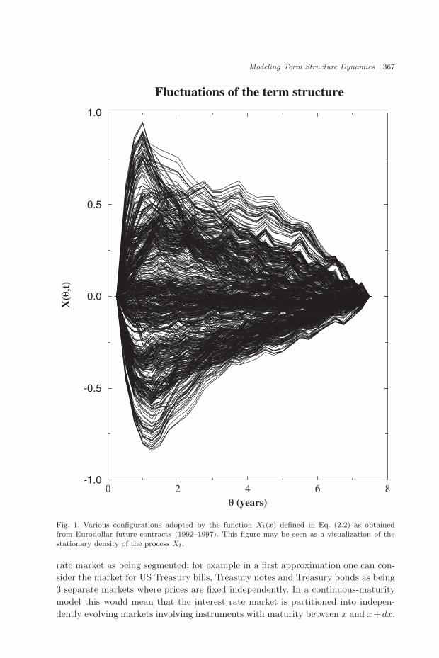
Figure 1 shows the various configurations adopted by the deformation processXt(x) in the case of Eurodollar futures.

In a Gaussian framework, the uncorrelated nature of the principal componentprocesses would entail their independence. In particular the first two principal com-ponents (which are roughly the spread and the short rate) would be independentfrom the deformation process Xt. However this assumption is not necessary in whatfollows and one can for example insert a state-dependent volatility or jump compo-nent in the short rate/spread process without altering the conclusions that follow.

2.3. The short rate and the spread

Among all interest rates, the short rate rt(xmin) is highly sensitive to the monetarypolicy of the central bank and cannot be considered as a market rate: its dynamics isexogenous to the fixed income market. One could therefore model its dynamics as anautonomous diffusion. However, as shown by Ait Sahalia [2], non-parametric teststend to reject the diffusion hypothesis for rt(xmin) taken individually whereas thehypothesis of a bivariate diffusion for (rt(xmin), s(t)) is not rejected. Motivated bythese remarks, we assume that the short rate and the long rate (rt(xmin), rt(xmax))are described by a (bivariate) Markov process.

drt(xmin) = µ1(rt(xmin), st) dt + σ1,1(rt(xmin), st) dZ1t + σ1,2(rt(xmin), st) dZ2

t ,

dst = µ2(rt(xmin), st) dt + σ2,1(rt(xmin), st) dZ1t + σ2,2(rt(xmin), st) dZ2

t ,

(2.5)


364 R. Cont

where Z1, Z2 are two independent noise sources, which can be Wiener processes ormore generally, may have discontinuous trajectories as observed in many empiricalstudies of short term interest rates. For example, the noise source in Eq. (2.5) couldbe replaced with a non-Gaussian Levy process without modifying what follows.Examples of diffusion models of this type have been previously considered in theliterature, see [7, 29].

2.4. Term structure deformations as infinite-dimensional

diffusions

We are now left with the deformation process (Xt)t≥0 to model. The first require-ment we impose on Xt is its smoothness in maturity: at a given time t, Xt is afunction defined on [xmin, xmax] determined by the forward term structure which,as remarked above, is a “smooth” function of the time to maturity x. Xt shouldtherefore belong to a suitable space H of smooth functions. In view of interpret-ing our results in terms of principal component analysis, we would like the statespace H to have a Hilbert structure in order to define orthogonal projections of Xt

onto a suitable basis of H .The second requirement we impose is that Xt be a Markov process in H . This

property, as remarked in [22], is already verified in the Heath-Jarrow-Morton [17]framework for the forward curve process ft. Together with the hypothesis of conti-nuity in time of the deformation process, this leads us to a diffusion model takingvalues in H . More precisely, stating that Xt is a H-valued diffusion process meansthat there exist a drift operator µ: H → H and a volatility operator σ: H → L2(H),defined on H , such that the evolution of Xt is given by a stochastic differential equa-tion in H :

dXt = µ(t, Xt) dt + σ(t, Xt) dBt, (2.6)

where Bt is a Brownian motion taking values in H . Here µ and σ may be allowedto depend on the contemporaneous term structure — they can be a function of thewhole curve Xt(x), x ∈ [xmin, xmax].

Formally, Eq. (2.6) is a stochastic differential equation in an (infinite-dimensional) function space H . In order to give a proper meaning to Eq. (2.6), oneshould start by specifying the nature of the random noise source Bt such that thestochastic integral implicit in Eq. (2.6) can be properly defined. There are severalways to define a generalization of the Wiener process and a stochastic integral in aninfinite dimensional space. The relation between these different constructions wasclarified by [33] who showed that the natural setting for constructing infinite dimen-sional diffusions is a Hilbert space. Here we give a brief survey of the mathematicalsetting in order to make it accessible to readers familiar with stochastic differentialequations in the finite dimensional setting. Given a (separable) Hilbert space H ,such as H = L2([xmin, xmax], ν) for some measure ν or an associated Sobolev spaceof smooth functions, and a complete orthonormal family (en)n≥1 of H , the elements



of H may be characterized by their decomposition on the basis (en)n≥1:

∀h ∈ H, ∃!(hn)n≥1,∑n≥1

h2n < +∞,

∣∣∣∣h −N∑

n≥1

hnen

∣∣∣∣H

−→N→∞

0. (2.7)

One would then like to define a “standard” Brownian motion in H as being asuperposition of independent scalar Wiener processes along each direction of thebasis:

Bt =∑n≥1

Wn(t)en. (2.8)

However, this sum does not converge in H since the coefficients in the expansionare not square summable: Bt cannot therefore be defined as a process taking valuesin H . However, for any unit vector h ∈ H the “projection” of Bt on h defines asquare integrable random variable:

Bt(h) := 〈Bt, h〉 =∑n≥1

Wn(t)hn ∈ L2(Ω, H). (2.9)

〈Bt, h〉 is in fact a scalar Brownian motion for each h and can be interpreted asthe component of Bt along h. This property may be used to define Bt through itsprojections: one can define a cylindrical Brownian motion on H as a family (Bt)t≥0

of random linear functionals Bt: H → R satisfying:

1. ∀h ∈ H,B0(h) = 0.

2. ∀h ∈ H,Bt(φ) is an Ft — adapted scalar stochastic process.3. ∀h ∈ H − 0, Bt(φ)

|φ| is a one-dimensional Brownian motion.

In particular, if one takes any orthonormal basis (en) in H then its image(Wn(t))t≥0 = (Bt(en))t≥0 forms a sequence of independent standard Wiener pro-cesses in R, which justifies the formal expansion (2.8). This property is indepen-dent of the choice of the orthonormal family (en). It is useful for building finite-dimensional approximations and is analogous to the construction of n-dimensionalBrownian motion as a vector of n independent scalar Wiener processes.

Although the expansion (2.8) does not converge in H , it can be made to convergeby weighting the terms with coefficients which decay with n:

WQt =

∑n≥1

Wn(t)qnen ∈ H, qn ≥ 0∑n≥1

q2n < ∞. (2.10)

The projections of WQ on the basis (en) still forms a sequence of independentWiener processes, but the variances q2

n now decay with n. This construction is notinvariant with respect to the choice of the basis (en)n≥1: a “change of basis” willintroduce correlations in the coordinates, with the covariances given by

cov(〈WQt , h1〉, 〈WQ

t , h2〉) = 〈Q · h1, h2〉, (2.11)


366 R. Cont

where Q is the symmetric positive operator defined by Q · en = qnen. WQ is calleda Q-Wiener process [9, 33]: it can be seen as a random field whose increments areuncorrelated in time but correlated in the x-direction.

The construction above can be carried out in any (separable) Hilbert spaceof functions: examples are weighted Sobolev spaces of real-valued functions on[xmin, xmax], i.e., the space of functions g ∈ L2([xmin, xmax], ν) such that the deriva-tive g(s) of order s is also in L2([xmin, xmax], ν). The Sobolev embedding theorem [1]then implies that if s > k + 1/2 then forward rate curves are k-times differentiablein the usual sense. Many recent papers have discussed other choices of state spacesfor forward rate curves (see, e.g., [14]): a typical requirement in these discussions isthat the forward rate is a continuous function of (time-to-)maturity so that pointevaluation x → rt(x) is a continuous operation. Note however that the instantaneousforward rates rt(x) are not observable quantities: the only observable quantities arezero-coupon bond prices or LIBOR rates. These quantities are integral functionalsof the forward rate curve, thus already continuous with respect to a weighted L2

norm. In the following we shall take as our state space H = L2([xmin, xmax], ν)and then give conditions under which the forward rate curve in our model actuallybelongs to Sobolev spaces Hs([xmin, xmax], ν) with a given smoothness s ≥ 1. Dueto the normalization used for the deformation process Xt, it actually verifies theboundary conditions (2.4) so we will see that Xt ∈ Hs

0([xmin, xmax], ν).At this level of generality, not much can be said of the properties of the solutions

of Eq. (2.6). In this section we will show how the description of term structure defor-mations through level, steepness and curvature of the yield curve reduces Eq. (2.6)to a stochastic partial differential equation, of which we study the simplest example.

2.5. Market segmentation and local deformations

As mentioned before, the maturity x is not simply a way to index different forwardrates and instruments: the fact that fixed income instruments are ordered by matu-rity is important for market operators. For example, this is reflected in the hedgingstrategies of operators on the fixed income market: to hedge an interest rate risk ofmaturity x = 8 months, an operator will tend to use bonds (or other fixed-incomeinstruments) of maturity close to 8 months: 6 months, 9 months. Although thisstrategy seems quite sensible, it does not correspond to the picture given by multi-factor models: in a k-factor model, any k + 1 instruments can be used to hedge aninterest rate contingent claim. For example in a two factor model one could use inprinciple a 30 year bond, a 10 year bond and a 6 year bond to hedge an instrumentwith maturity of two years! Needless to say, no sensible trader would follow such astrategy, which shows that in practice the factors which explain 95% of the varianceare not enough to hedge 95% of the risk of an instrument with a non-linear payoff:this is precisely our principal motivations for introducing maturity-specific sourcesof randomness.

The existence of maturity-specific risk naturally leads to a market for such risk.Indeed, some macroeconomic theories of interest rates have considered the interest



Fig. 1. Various configurations adopted by the function Xt(x) defined in Eq. (2.2) as obtainedfrom Eurodollar future contracts (1992–1997). This figure may be seen as a visualization of thestationary density of the process Xt.

rate market as being segmented: for example in a first approximation one can con-sider the market for US Treasury bills, Treasury notes and Treasury bonds as being3 separate markets where prices are fixed independently. In a continuous-maturitymodel this would mean that the interest rate market is partitioned into indepen-dently evolving markets involving instruments with maturity between x and x+dx.


368 R. Cont

However this is not strictly true: as shown by principal component analysis, long-term rates do react to variations in the short rate in a way that is not explainablesimply via parallel shifts and vertical dilations of the term structure. One way toconciliate the interdependence of rates of various maturities with the segmentationof markets across maturities is by considering deformations of the term structurethat are local in maturity: a forward rate of maturity x is more sensitive to variationsof rates with maturity close to x. We are not dealing here with a strict segmentationof the market into separately evolving markets but a “soft” segmentation whichsimply implies that the market for each maturity adjusts itself to the variation inrates of maturities immediately above and below it. This means for example that,among all rates of maturity ≥1 year, the 1 year rate will have a higher sensitivityand react more quickly to a variation in the short rate since it is closer in maturity.

2.6. Level, steepness and curvature

In mathematical terms, the local deformation hypothesis means that the variationof Xt(x) will only depend on the behavior of Xt(·) around x. One can parameterizethe shape of the term structure around a given maturity x by its first few derivatives:Xt(x), ∂xXt, ∂2

xXt, . . . As noted before, empirical studies seem to identify the level ofinterest rates, the steepness (slope) of the term structure and its curvature as threesignificant parameters in the geometry of the yield curve [20]. In a market involvinginstruments of maturity between x and x + dx, these three features are describedby the level of rates, and the first two derivatives with respect to x. Combiningthe local deformation hypothesis formulated in Sec. 5.1. with a local description ofthe term structure by level, steepness and curvature one obtains that the drift andvolatility of Xt(x) can only depend on Xt(x), ∂xXt, ∂2

xXt. Econometric evidencefor the influence of the local slope and level on the movements of forward rates hasbeen observed by [25] among others. Equation (2.6) then becomes a second orderstochastic partial differential equation:

dXt =[∂Xt

∂x+ b

(Xt(x),

∂Xt

∂x,∂2Xt

∂x2

)]dt + σ

(Xt(x),

∂Xt

∂x,∂2Xt

∂x2

)dBt(x),

∀ t ≥ 0, Xt(xmax) = Xt(xmin) = 0, Xt=0(x) = X0(x). (2.12)

This equation is the mathematical expression of the fact that deformations are localin maturity and that the deformation at maturity x depends on the level, steepnessand curvature of the term structure around x.

As noted by [16, 22], HJM models also give rise to (first-order) stochastic PDEsfor risk-neutral dynamics of the term structure. The new aspect in our approachis the inclusion of a second order term which captures the effect of curvature andchanges the nature of the equation. In the general case where b and σ are nonlinearfunctions of their arguments, Equation (2.12) is not easy to study: indeed, it is nottrivial to define properly what is meant by a solution of Eq. (2.12) and even less tostudy their regularity [9, 24]. In order to point out the differences with HJM-type



models resulting from the local deformation hypothesis, we shall consider the caseof a forward rate dynamics such as (1.2) which is perturbated by a term dependingon the curvature:

dXt =[∂X

∂x+ b(t, x, Xt(x)) +

κ

2∂2X

∂x2

]dt + σ(t, x, Xt(x)) dBt(x),

∀ t ≥ 0, Xt(xmin) = Xt(xmax) = 0, Xt=0(x) = X0(x). (2.13)

Mathematical properties of stochastic PDEs such as Eq. (2.13) have been widelystudied in the mathematical literature: see [9, 18, 24, 32]. The approach adoptedhere is that of [9]. In the following section we study the simplest case where volatilityis constant; surprisingly, we will show that this simple case already presents manyof the desirable features enumerated in Sec. 1.

3. The Linear Parabolic Case

In order to illustrate what are the type of dynamics implied by Eq. (2.13) forterm structure deformations, we will now study the simplest example of the aboveequations which incorporates the influence of local steepness and curvature, namelythe case where σ is independent of Xt. For the sake of simplicity we will deal herewith the constant volatility case but all the results below remain valid in the case ofan arbitrary deterministic function of time t. The case of constant volatility leadsus to the following stochastic partial differential equation:

∂X

∂t=

[∂X

∂x+

κ

2∂2X

∂x2

]dt + σ0 dBt(x), (3.1)

∀ t ≥ 0, Xt(xmin) = Xt(xmax) = 0, (3.2)

∀x ∈ [xmin, xmax], Xt=0(x) = X0(x). (3.3)

3.1. Eigenmodes and principal components

Let x∗ = xmax − xmin be the maturity span of the observed forward rate curve. Bytranslating the maturity variable one can assume xmin = 0 without loss of generalityin what follows. We consider as state space for our solutions the Hilbert space H ofreal-valued functions defined on [0, x∗] with the scalar product:

〈f, g〉H =∫ x∗

0

dx exp(

2x

κ

)f(x) g(x). (3.4)

The subscript H in 〈., .〉H will be omitted in most of this section. Let A be theoperator in H defined by:

A · u =∂u

∂x+

κ

2∂2u

∂x2. (3.5)

It is not difficult to show that A has a discrete spectrum, with eigenvalues andeigenfunctions given by:

A · en = −λnen, (3.6)


370 R. Cont

λn =12κ

(1 +

n2π2κ2

x∗2

), (3.7)

en(x) =

√2x∗ sin

(nxπ

x∗)

exp(−x

κ

), (3.8)

where n takes all integer values ≥ 1. Here the eigenfunctions en have been normal-ized such that (en)n≥1 is an orthonormal basis of H .

〈en, em〉 = δnm. (3.9)

The functions (eigenmodes) en(x) play the role of the principal components for thedeformation process Xt. That is, if we perform a principal component analysis ona realization of the process Xt, for a large enough sample the empirical principalcomponents would reproduce the eigenmodes en(x). The first two of these eigen-modes are shown in Fig. 2. The role of the exponential term in Eq. (3.8) is clearlyvisible: the eigenfunctions become “skewed” towards shorter maturities and onlya single hump, whose position is determined by the value of κ, is visible. Recallthat this exponential term stems simply from the fact that we are parameterizingthe forward rate process by time to maturity x instead of maturity date T [22].In particular, in contrast with multifactor models [21], there is no need to use acomplicated volatility structure σ(t, x) to obtain a volatility hump. The position ofthe hump gives a (first) simple method for estimating the value of κ from empiricalobservations. Remark also that the exponential factor prevents more than one humpfrom appearing in the eigenfunctions: as a result, multi-humped deformations arenot observed, in concordance with the empirical observations invoked in Sec. 2.

Fig. 2. First two eigenmodes of the operator A, with κ = 4 and x∗ = 30 years. Note the maximasituated at short maturities.



The Green function (propagator) associated to the operator A may then beexpressed in terms of an eigenmode expansion:

G(t, x, y) =∑n≥1

exp(−λnt)en(x)en(y). (3.10)

The random field Xt(x) is then said to be a mild solution [9] of Eq. (3.1) if it verifiesthe equation in the following integral form:

Xt(x) =∫ x∗

0

G(t, x, y)X0(y) dy +∫ t

0

ds

∫ x∗

0

G(t − s, x, y)σ0dBs(y). (3.11)

Let Xt(x) be the solution of Eq. (3.11). Define the coordinates of the solution inthe eigenvector basis as:

xn(t) = 〈Xt, en〉 =∫ x∗

0

dxXt(x)en(x) exp(

2x

κ

). (3.12)

The coefficients xn(t) therefore represents the projection of the deformation processXt on the nth principal component (eigenmode). For each n, xn(t) is then a solutionof a linear stochastic differential equation:

dxn(t) = −λnxn(t) dt + σ0 dWnt , (3.13)

where Wnt = Bt(en) are independent standard Wiener processes. (xn(t))n≥1 there-

fore constitute a sequence of independent Ornstein–Uhlenbeck processes. TheOrnstein–Uhlenbeck process is the process used to represent the short rate in theVasicek model [31]: it possesses the fundamental property of mean reversion whichhas made it a popular model in interest-rate modeling. In our case, this meanreversion is observed in the principal components of the yield curve: while individ-ual forward rates may have a non-stationary and irregular behavior the yield curveas a whole will converge to a stationary state with a mean-reverting behavior. Wecan thus represent the random field Xt(x) as an infinite factor model where eachfactor follows an Ornstein–Uhlenbeck process:

Xt(x) =∑n≥1

xn(t)en(x), (3.14)

xn(t) = e−λnt〈en, X0〉 +∫ t

0

ds e−λn(t−s)σ0dWns . (3.15)

Equation (3.17) has an interesting interpretation. Remember that xn(t) the projec-tion of the deformation process Xt on the nth principal component. Equation (3.15)expresses xn(t) as the sum of two components, the first one being the contribu-tion of the initial term structure to xn and the second one its stationary value.Equation (3.15) may then be interpreted by stating that the forward rate curve“forgets” the contribution of the nth principal component to the initial term struc-ture at an exponential rate with characteristic time

τn =1λn

=2κ

1 + n2π2κ2

x∗2

. (3.16)

Therefore, a perturbation of the initial term structure due to the nth principalcomponent will disappear or be smoothed out after a typical time τn which decreases


372 R. Cont

with n: perturbations which have an irregular profile in maturity die out morequickly than smoother ones. This property guarantees that in the long term onlysmooth deformations of the term structure remain visible, which guarantees thesmoothness in maturity and shows the important relation between the smoothingproperty of the operator A and the decay of its eigenvalues: an operator with aquickly decaying spectrum will guarantee a fast decay (in time) of the singularitiesappearing in the term structure and restore smoothness in maturity. This gives asecond interpretation of the parameter κ: in addition to determining the position ofthe volatility hump, it also determines the decay rate of perturbations of the termstructure. This interpretation gives a second, independent method for estimatingthe model parameters from empirical data. One can also construct more generalmodels where these two roles of κ can be attributed to two separate parameters byintroducing a term structure κ(x) [8].

The factor representation (3.14) can be easily generalized to the case wherefactors have unequal volatilities (σn, n ≥ 1):

xn(t) = e−λnt〈en, X0〉 +∫ t

0

ds e−λn(t−s)σn dWns . (3.17)

Xt is then the (mild) solution of

dXt = A · Xt dt + σ · dBt, (3.18)

where σ is now an operator verifying

σ · en = σ2nen, σ · A = A · σ. (3.19)

Given the explicit form of λn, it is easily verified that the series

E[Xt(x)] =∑n≥1

e−λnt〈X0, en〉en(x), (3.20)

Var[Xt(x)] =∑n≥1

σ2n

1 − exp(−2λnt)2λn

en(x)2, (3.21)

are absolutely convergent for all (t, x) and (3.14) defines a Gaussian random fieldwith mean and variance given by (3.20)–(3.21).

3.2. Average term structure and mean reversion

Under the above assumptions, one can calculate the average shape of the termstructure of forward rates from Eq. (2.2).

E[rt(x)] = E[rt(xmin)] + E[s(t)]Y (x). (3.22)

The shape function Y (x) can therefore be chosen in order to reproduce the averageterm structure. Bouchaud et al. [5] propose the following shape function:

Y (x) =√

x

x∗ , (3.23)



which appears to give a good fit of the average shape of the Eurodollar term struc-ture for maturities ranging from 3 months to 10 years [5]. However, the preciseanalytic form of the shape function Y does not affect the results above.

How does the yield curve fluctuate around its average shape? It is easily seenfrom Eq. (3.21) that the process Xt converges for t → ∞ to a Gaussian randomfield X∞ with mean zero and covariance:

Cov(Xt(x), Xt′ (x′)) =∑n≥1

σ2n

en(x)en(x′)e−λn(t−t′)

2λn. (3.24)

Viewed as a process in H , (Xt) is an Ornstein Uhlenbeck process whose stationarydistribution is a Gaussian distribution with covariance

C =12σ · σ∗A−1, with spectral decomposition C · en =

σ2n

2λnen, n ≥ 1. (3.25)

An important consequence of Eq. (3.25) is that the variance of the principal com-ponents can be small without the factor volatilities being small: a fast increase ofλn has the effect of damping out the variance of the higher principal components.In terms of term structure movements, stationarity of term structure deformationsimplies a mean-reverting behavior of forward rates. The analytic form of the sta-tionary measure further allows to compute the probability of a given yield curvedeformation by decomposing it on the principal component basis.

3.3. Smoothness in maturity

As mentioned above, an important property of forward curves is their smoothnessin maturity x, as opposed to their irregular behavior in t. In the parabolic SPDEmodel, this property is guaranteed by the smoothing effect of the second orderderivative in x. Moreover, one can precisely relate the rate of decay of volatilitiesσn of the factors to the smoothness of the forward rate curve:

Proposition 3.1. If the volatilities σn decay faster than n−β i.e., (nβσn)n≥1 isbounded then, with probability 1, the stationary solution of (3.18)–(3.19) is k timesdifferentiable with respect to the maturity variable x for every k < β.

Proof. Let P∞ be the stationary distribution of Xt on L2([xmin, xmax], ν). P∞is a Gaussian measure with covariance C where C = A−1 · σ∗σ/2. So C · en =σ2

n/2λn. Now assume σn = ann−β with (an) bounded and take k < β. Then,EP∞ |〈Xt, en〉|2 = σ2

n/2λn. Now take any real number s > k + 1/2. The Sobolevspace Hs([xmin, xmax]) is defined by

h ∈ Hs ⇔ h ∈ L2([xmin, xmax], ν), |h|2Hs =∑n≥1

n2s|〈h, en〉|2 < +∞.

Substituting h = Xt and taking expectations one obtains

EP∞‖Xt‖2Hs =

∑n≥1

n2sσ2

2λn=

∑n≥1

ann2s−2β

2λn.


374 R. Cont

Since λn increases as n2, the summands are bounded by a sequence decaying asn2s−2−2β . So 2s − 2 − 2β < −1 and the series is absolutely convergent:

EP∞‖Xt‖2Hs < +∞.

Therefore P∞(‖Xt‖2Hs < +∞) = 1 so ∀ s > k+ 1

2 , P∞(Xt ∈ Hs) = 1. By the Sobolevembedding theorem [1], every element of Hs, s > k + 1/2 is k times differentiablewith respect to x hence the result.

This result means that one can then read off the degree of smoothness of the for-ward rate curve from the decay rate of factor volatilities, in a very simple way.In particular, if the number of driving factors is finite, the forward rate curve isinfinitely differentiable in x.

It also implies that we can read off the degree of differentiability with respect tomaturity from the rate of decay of variances in the principal component analysis: ifthe variances decay as n−β, then the maximal degree of differentiability of forwardrate curves is less than β. Empirical studies [5] indicate a rate of decay betweenβ = 2 and β = 3. However β is the asymptotic rate of logarithmic decay and assuch may be difficult to determine precisely from empirical data since by definitionone has observations on a discrete tenor of maturities. This point is also discussedby [10].

Note finally that, even in the case of flat term structure where σ = σ0I, in whichcase the noise term is space-time white noise, the dependence in maturity x is stilltwice as smooth as in t: the asymmetry between t and x dependence is not due toan ad-hoc choice of volatility structure [21] or of the noise source (as [28], see below)but is a generic property due to the presence in (3.1) of the second derivative withrespect to maturity.

3.4. Random strings: parabolic vs. hyperbolic formulation

In a recent work [28], it has been proposed to consider stochastic partial differentialequations of hyperbolic type to describe the evolution of the forward rate curve.Such an equation differs from the above one through the presence of a second-ordertime derivative which dominates the dynamics. The hyperbolic model proposed by[28] is formulated in terms of the forward rate process itself (in the spirit of theHJM model [17]) and not in terms of the deformation process Xt, by examining theeffect of a second-order time derivative in the equations of Sec. 5. Let us thereforeconsider the general case where the evolution equation contains both a propagationterm and a diffusion term:

f∂2X

∂t2+

∂X

∂t=

∂X

∂x+

κ

2∂2X

∂x2+ σ · dBt(x), (3.26)

∀ t ≥ 0, Xt(0) = Xt(x∗) = 0, (3.27)

Xt=0(x) = X0(x),∂Xt=0

∂t= Y0. (3.28)



The above equation is analogous to that of a vibrating elastic string, hence the nameof “string models” given to such descriptions of term structure movements. The casef = 0 is the one studied in Sec. 5; the case f → ∞ (the other parameters beingappropriately rescaled) is the stochastic wave equation [9], the “space” variablebeing x+ t. Note that the stochastic PDE proposed by [28] is formulated as a PDEperturbated by a two-parameter (“space-time”) noise (called a “stochastic stringshock”) while our Eq. (3.1) or the general case Eq. (2.12) was presented above asan evolution equation for a curve in some function space. In the case of a parabolicSPDE, where only the first derivative with respect to time is involved, the twoapproaches are equivalent for a two-parameter process. Choosing one approach orthe other then amounts to viewing the solution of a stochastic PDE either as arandom field or as a stochastic process in a function space. Implicit in this choiceis whether the object of interest for modeling purposes is an individual interestrate or the deformation of a multivariate object, namely the term structure. Theparabolic equation in Sec. 3 has the merit of emphasizing the asymmetric roles ofthe variables x and t, an empirically desirable feature which is not present, as weshall see below, in the hyperbolic case.

Manifestly, the operator on the right hand side of Eq. (3.26) is the same as inEq. (3.1). This means that the deformation eigenmodes (the eigenfunctions of A)will remain the same as in Eq. (3.1) studied above but the projection of the processXt on each of them will be different. For example, a stationary solution of Eq. (3.26)will not give the same weight to the eigenmodes as in the parabolic case studiedin Sec. 5 and therefore the results of a Principal Component Analysis of Eq. (3.26)will differ from that of Eq. (3.1) in terms of the eigenvalues.

The representation of the equation in terms of its projections on the eigenmodebasis en gives as above a stochastic equation for the scalar process yn(t) = 〈Xt, en〉:

fd2yn

dt2+

dyn

dt= −λnyn(t) + σ0W

nt . (3.29)

This formal second-order stochastic differential equation is interpreted in the usualway, as follows. Consider the Green function Un(t) of the operator f ∂2u

∂t2 + ∂u∂t +λnu,

given by:

Un(t) =1

f√

1 − 4λnf[er1,nt − er2,nt]1t>0, (3.30)

where r1,n and r2,n being the roots of the associated characteristic equation:

fr2 + r + λn = 0. (3.31)

The process xn(t) is then given by the stochastic convolution integral:

yn(t) = ane−r1,nt + bne−r2,nt +∫

Un(t − s) dWns , (3.32)

which is well-defined since the integrator is square-integrable in s. Here an andbn are defined by the initial conditions. Depending on the values of f and κ, two


376 R. Cont

scenarios are possible:

1. Oscillatory behavior: if

f >κ

2(1 + π2κ2

x∗2

) , (3.33)

then for all n ≥ 1, Eq. (3.31) has two complex conjugate roots given by:

r1,n =i√

4λnf − 1 − 12f

= − 12f

+ iωn, (3.34)

r2,n =−i

√4λnf − 1 − 1

2f= − 1

2f− iωn. (3.35)

The real part gives an exponential damping of the initial conditions which char-acterizes the mean reverting behavior of Xt as in the parabolic case. First remarkthat, unlike the parabolic case where “bumpy” principal components which con-tribute the most to non-smoothness in maturity decay more quickly, here allprincipal components decay with the same speed, i.e., a mean reversion time of2f . Recall that κ still determines the position of the volatility hump so κ 1year. So (3.33) implies that f > 6 months. The mean reversion time of the wholecurve is thus around a year. However, a new phenomenon appears: the principalcomponents do not simply revert to their mean but oscillate around their meanwith a frequency ωn/2π which increases with n:

xn(t) = Ane−t/2f cos(ωnt + φn). (3.36)

The phase φn and amplitude factor An are determined by (two) initial conditions(see below). The oscillation of the term structure around its mean is not neces-sarily an undesirable feature of this model and indeed can be justified on eco-nomic grounds [8]. But the slow mean reversion combined with increasingly fasteroscillations of the higher order principal components leads to non-smoothness inmaturity of the solutions of Eq. (3.26) [9]: in fact one should expect the cross-sections in time or maturity to have the same irregularity which, as pointed outin Sec. 1, is not a desirable feature for a term structure model.

2. Selective damping of principal components: if

f <κ

2(1 + π2κ2

x∗2

) , (3.37)

then ∃N > 1 such that for n ≤ N , Eq. (3.31) has two real, negative rootswhereas for n > N the roots are complex conjugates with negative real parts.The projections of the deformations process Xt on the first N eigenmodes willhave a mean reverting behavior as in the parabolic case,1 with a mean reversiontime increasing with n. For n > N , xn(t) will have a damped oscillatory behavior,

1In fact the decay of the initial condition is described in this case by the superposition of twodecreasing exponentials with time constants given by r−1

1n and r−12n .



with a damping time τ = 2f independent of n and an oscillation frequencyincreasing with n as above.

Another crucial difference between Eq. (3.26) and Eq. (3.1) is the nature of theinitial conditions. In the case of the parabolic equation (3.1) the problem has awell defined solution once the initial term structure is specified through X0. Thisis not sufficient in the case of Eq. (3.26): one must also specify the derivative withrespect to time at t = 0. In the case of a vibrating string, this means specifying theinitial position and the initial velocity of each point of the string. For a model ofthe forward rate curve, this can be inconvenient: while the initial term structure isthe natural input for the initial condition of a dynamic model, the time derivativeof the forward rates is not easily evaluated, especially given the irregularity in timeof forward rate trajectories which prevents such a model from being calibrated in anumerically stable manner.

We therefore conclude that the question of including a second-order time deriva-tive in Eq. (3.26) is not simply a matter of taste: its radically changes both thedynamic properties of the equation and the nature of the initial conditions neededto calibrate the model, in an empirically undesirable fashion. Our analysis thuspleads for a description of yield curve deformations through a parabolic rather thanhyperbolic SPDE.

4. Conclusion and Perspectives

We have presented a parsimonious stochastic model for describing the fluctuationsof the term structure of forward rates: the forward rate curve is described as arandom curve oscillating around its long term average or, alternatively, as randomfield solution of a stochastic PDE. The model studied in Sec. 3 should be viewedas the simplest example of model incorporating the effect of slope and curvature inforward rate dynamics. However this simple example has the benefit of emphasiz-ing the role of the second derivative with respect to maturity in the evolution ofthe term structure: indeed, as we have seen above, it is this second derivative whichtames the maturity-specific randomness and maintains a regularity in x while allow-ing for independent shocks along maturities. It also gives the correct form for theprincipal components as well as a qualitatively correct estimate for their associatedeigenvalues. These results show the importance of the concept of local deformationexplained in Sec. 2.5, of which our equation is the simplest example. The model inSec. 3 can be generalized to the case of state and time-dependent coefficients [8] butthe point is that a linear model with constant coefficients and flat term structureof volatility is already sufficient for reproducing empirical facts which, in standardinterest rate models, need fine tuning of many parameters. Let us recall our mainresults:

1. The linear parabolic SPDE (3.1) reproduces the qualitative form of the principalcomponents, the presence of a humped volatility term structure and the mean


378 R. Cont

reverting properties of forward rates with two parameters and without insertingad-hoc structures in the noise terms.

2. The term structure deformation solution of (3.1) may be represented as aGaussian random field Xt(x), as an infinite-factor model (3.14) with Ornstein-Uhlenbeck dynamics for the factors or as a diffusion Xt in a space of curves.

3. A large (or infinite) number of factors is compatible with the fact that a fewprincipal components capture most of the variance. The decay in the variance ofprincipal components results from the smoothing effect of the evolution operatorand is due to the impact of the curvature (convexity) on forward rate dynamics.

4. We do not require a humped term structure for the diffusion coefficient σ in orderto obtain a humped term structure for the volatilities of the forward rates: in facta flat term structure for σ already generates this hump in standard deviationsof forward rate movements.

5. The model provides a link between the geometry of the forward rate curve —its shape and smoothness, measures by the principal components and their vari-ances — and the dynamics, i.e., the time series properties of forward rates, asmeasures by their mean reversion time and autocorrelation properties. Both setsof properties are governed by the same parameters.

As mentioned in the introduction, our objective has been to obtain a faithfulcontinuous-time representation of the statistical properties of the forward rate curve.Obviously such a model can be useful for simulating realistic scenarios for yield curvemovements. It remains to establish the link with the arbitrage pricing approach andexamine the consequences of our model for hedging interest rate options. As shownby [4], such an analysis requires a careful specification of the class of strategies oneis willing to consider; also, as noted by [5], taking into account transaction costseliminates theoretical “arbitrage opportunities” present in a model such as (3.1).These issues remain to be explored in more detail.

A remaining question is to explain the economic origin for the second-order termin (3.1). We discuss this issue in a forthcoming work [8].

Acknowledgments

Part of this work was done while the author was a research fellow at the SwissFederal Institute of Technology, Lausanne (EPFL) in 1998. I thank Toufic Abboud,Jean-Philippe Bouchaud, Rene Carmona, Robert Dalang, Nicole El Karoui, DamirFilipovic, Vincent Lacoste, Olivier Leveque, Carl Mueller, Francesco Russo, JerzyZabczyk, Shiva Zamani and seminar participants at Universite de Paris XIII, EcolePolytechnique, EPFL, Princeton University, Seminaire Bachelier (Paris), Olsen &Associates, HEC Montreal, University of Copenhagen, INRIA Sophia Antipolis andINRIA Rocquencourt for useful remarks and encouragement. All remaining errorsare mine.



References

[1] R. A. Adams, Sobolev Spaces (Academic Press, New York, 1975).[2] Y. Ait-Sahalia, Telling from discrete data whether the underlying continuous-time

model is a diffusion, Journal of Finance 57 (1977) 2075–2112.[3] G. Ballocchi, M. M. Dacorogna, C. M. Hopman, U. A. Muller and R. B. Olsen, The

intraday multivariate structure of the Eurofutures markets, Journal of EmpiricalFinance 6 (1999) 479–513.

[4] T. Bjork, G. Di Masi, Y. Kabanov and W. Runggaldier, Towards a general theory ofbond markets, Finance and Stochastics 1(2) (1997) 141–174.

[5] J. P. Bouchaud, R. Cont, N. El Karoui, M. Potters and N. Sagna, Phenomenology ofthe interest rate curve, Applied Mathematical Finance 6 (1999) 209–231.

[6] J. P. Bouchaud, R. Cont, N. El Karoui, M. Potters and N. Sagna, Strings attached,RISK (July 1998).

[7] M. J. Brennan and E. J. Schwartz, A continuous-time approach to the pricing ofbonds, Journal of Banking and Finance 3 (1979) 133–155.

[8] R. Cont, A structural model for term structure dynamics, working paper (2003).[9] G. Da Prato and J. Zabczyk, Stochastic Equations in Infinite Dimensions (Cambridge

University Press, 1992).[10] R. Douady, Yield curve smoothing and residual variance of fixed income positions,

working paper (1997).[11] D. Duffie and R. Kan, Multifactor models of the term structure, in Mathematical

Models in Finance, eds., Howison, Kelly and Wilmott (Chapman & Hall, London,1995).

[12] P. Dybvig, J. Ingersoll and S. Ross, Long forward and zero-coupon rates can neverfall, Journal of Business 69 (1996) 1–26.

[13] N. El Karoui, A. Frachot and H. Geman, A note on the behavior of long zerocoupon rates in a no arbitrage framework, Review of Derivatives Research 1(4) (1998)351–369.

[14] D. Filipovic, Consistency Problems for Heath-Jarrow-Morton Models, Lecture Notesin Mathematics Vol. 1760 (Springer, Berlin, 2000).

[15] R. Goldstein, The term structure of interest rates as a random field, Review of Finan-cial Studies 13(2) (2000) 365–384.

[16] B. Goldys and M. Musiela, Infinite dimensional diffusion, Kolmogorov equations andinterest rate models, in Option Pricing, Interest Rates and Risk Management, eds.,E. Jouini and S. Pliska (Cambridge University Press, 2001).

[17] D. Heath, R. A. Jarrow and A. Morton, Bond pricing and the term structure ofinterest rates: A new methodology for contingent claims valuation, Econometrica 60(1992) 77–105.

[18] K. Ito, Stochastic Differential Equations in Infinite Dimensions (SIAM, Providence,1984).

[19] D. P. Kennedy, The term structure of interest rates as a Gaussian random field,Mathematical Finance 4 (1994) 247–258.

[20] R. Litterman and J. Scheinkman, Common factors affecting bond returns, Journal ofFixed Income 1 (1991) 49–53.

[21] J. Moraleda, On the pricing of interest rate options, Ph.D. thesis, Tinbergen InstituteResearch Series, Vol. 155 (1997).

[22] M. Musiela, Stochastic PDEs related to term structure models, preprint (1993).[23] H. Pages, Interbank interest rates, in Mathematical Finance: Theory and Practice,

Series in Contemporary Applied Mathematics, eds., R. Cont and J. Yong (HigherEducation Press, Beijing, 2000), pp. 317–352.


380 R. Cont

[24] E. Pardoux, Stochastic partial differential equations: A review, Bulletin des SciencesMathematiques 117(1) (1993) 29–47.

[25] N. Pearson and A. Zhou, A non-parametric analysis of the forward rate volatilities,in The New Interest Rate Models, ed., L. Hughston (Risk Books, London, 2001).

[26] S. Pliska, Introduction to Mathematical Finance (Blackwell Publishers, 1997).[27] R. Rebonato, Interest Rate Option Models (Wiley, Chichester, 1997).[28] P. Santa Clara and D. Sornette, The dynamics of the forward interest rate curve with

stochastic string shocks, Review of Financial Studies 14(1) (2000), 149–185.[29] D. Schaefer and E. Schwartz, A two factor model for the term structure: An approx-

imate analytical solution, Journal of Financial and Quantitative Analysis 19 (1984)413–424.

[30] E. Schlogl and D. Sommer, Factor models and the shape of the term structure, Journalof Financial Engineering 7(1) (1998) 79–88.

[31] O. Vasicek, An equilibrium characterization of the term structure, Journal of Finance5 (1977) 177–188.

[32] J. B. Walsh, An introduction to stochastic partial differential equations, in Ecoled’Ete de Probabilite de Saint-Flour, Session XIV, Lecture Notes in Mathematics1180 (Springer, Berlin, 1986).

[33] M. Yor, Existence et unicite de diffusions a valeurs dans un espace de Hilbert, Annalesde l’Institut Henri Poincare 10 (1974) 55–88.

MODELING TERM STRUCTURE DYNAMICS: AN INFINITE …rama/papers/IJTAF.pdf · Modeling Term Structure...

Documents

Transcript of MODELING TERM STRUCTURE DYNAMICS: AN INFINITE …rama/papers/IJTAF.pdf · Modeling Term Structure...