Modeling, System Identification, and Control for

Dynamic Locomotion of the LittleDog Robot on

Rough Terrain

by

Michael Yurievich Levashov

B.S. Aerospace Engineering,B.S. Physics

University of Maryland (2008)

Submitted to the Department of Aeronautics and Astronauticsin partial fulfillment of the requirements for the degree of

Master of Science in Aeronautics and Astronautics

at the

MASSACHUSETTS INSTITUTE OF TECHNOLOGY

February 2012

c© Massachusetts Institute of Technology 2012. All rights reserved.

Signature of Author . . . . . . . . . . . . . . . . . . . . . . . . . . . . . . . . . . . . . . . . . . . . . . . . .Department of Aeronautics and Astronautics

September 21, 2012

Certified by. . . . . . . . . . . . . . . . . . . . . . . . . . . . . . . . . . . . . . . . . . . . . . . . . . . . . . . . . .Russ L. Tedrake

Associate Professor of Computer Science and EngineeringThesis Supervisor

Accepted by . . . . . . . . . . . . . . . . . . . . . . . . . . . . . . . . . . . . . . . . . . . . . . . . . . . . . . . . .Eytan H. Modiano

Associate Professor of Aeronautics and AstronauticsChair, Graduate Program Committee

Modeling, System Identification, and Control for Dynamic

Locomotion of the LittleDog Robot on Rough Terrain

by

Michael Yurievich Levashov

Submitted to the Department of Aeronautics and Astronauticson September 21, 2012, in partial fulfillment of the

requirements for the degree ofMaster of Science in Aeronautics and Astronautics

Abstract

In this thesis, I present a framework for achieving a stable bounding gait on theLittleDog robot over rough terrain. The framework relies on an accurate planar modelof the dynamics, which I assembled from a model of the motors, a rigid body model,and a novel physically-inspired ground interaction model, and then identified using aseries of physical measurements and experiments. I then used the RG-RRT algorithmon the model to generate bounding trajectories of LittleDog over a number of sets ofrough terrain in simulation. Despite significant research in the field, there has beenlittle success in combining motion planning and feedback control for a problem thatis as kinematically and dynamically challenging as LittleDog. I have constructeda controller based on transverse linearization and used it to stabilize the plannedLittleDog trajectories in simulation. The resulting controller reliably stabilized theplanned bounding motions and was relatively robust to significant amounts of timedelays in estimation, process and estimation noise, as well as small model errors. Inorder to estimate the state of the system in real time, I modified the EKF algorithmto compensate for varying delays between the sensors. The EKF-based filter worksreasonably well, but when combined with feedback control, simulated delays, and themodel it produces unstable behavior, which I was not able to correct. However, theclose loop simulation closely resembles the behavior of the control and estimationon the real robot, including the failure modes, which suggests that improving thefeedback loop might result in bounding on the real LittleDog. The control frameworkand many of the methods developed in this thesis are applicable to other walkingsystems, particularly when operating in the underactuated regime.

Thesis Supervisor: Russ L. TedrakeTitle: Associate Professor of Computer Science and Engineering

3

Acknowledgments

I want to thank my adviser, Russ Tedrake, for having me as a student in his lab

and providing me with the opportunity to do research in one of the best academic

environments in the world. His teaching and guidance were invaluable during my

time in the Robot Locomotion Group.

I want to also thank Alek Shkolnik, with whom I closely worked on LittleDog. He

was extremely helpful in bringing me up to speed with the robot, we shared many

ideas and lines of code for our research, and his ability to quickly hack together code

worked well in combination with my thoroughness.

The Robot Locomotion Group has a great intellectual atmosphere, a can-do at-

titude, and is full of brilliant and always willing to help people. I want to thank all

of the current and former members of RLG who helped me flesh out ideas, explained

and discussed control algorithms, or even just temporarily took my mind off work

with a random math problem.

Finally, I want to thank my family and friends for always supporting me in my

pursuit of higher learning.

4

Contents

1 Introduction 9

1.1 Motivation . . . . . . . . . . . . . . . . . . . . . . . . . . . . . . . . . 9

1.2 State of Legged Locomotion . . . . . . . . . . . . . . . . . . . . . . . 10

1.3 LittleDog . . . . . . . . . . . . . . . . . . . . . . . . . . . . . . . . . 12

1.4 Contributions . . . . . . . . . . . . . . . . . . . . . . . . . . . . . . . 14

2 Framework 15

3 Model 19

3.1 Motor Model . . . . . . . . . . . . . . . . . . . . . . . . . . . . . . . 21

3.2 Ground Interaction Model . . . . . . . . . . . . . . . . . . . . . . . . 23

3.2.1 Terrain Model and Foot Roll . . . . . . . . . . . . . . . . . . . 24

3.2.2 Ground Friction Model . . . . . . . . . . . . . . . . . . . . . . 25

3.2.3 Ground Forces Computation . . . . . . . . . . . . . . . . . . . 26

3.3 Parameter Estimation . . . . . . . . . . . . . . . . . . . . . . . . . . 29

3.3.1 Model Performance . . . . . . . . . . . . . . . . . . . . . . . . 31

4 State Estimation 35

4.1 LittleDog Sensor and Control Environment . . . . . . . . . . . . . . . 35

4.2 Extended Kalman Filter with Time Delays . . . . . . . . . . . . . . . 37

4.3 Modified Dynamics Model . . . . . . . . . . . . . . . . . . . . . . . . 40

4.4 Estimator Performance . . . . . . . . . . . . . . . . . . . . . . . . . . 42

5

5 Feedback Control 43

5.1 Transverse Linearization . . . . . . . . . . . . . . . . . . . . . . . . . 43

5.1.1 Transverse Linearization on Continuous Systems . . . . . . . . 43

5.1.2 Orthogonal Surfaces . . . . . . . . . . . . . . . . . . . . . . . 46

5.1.3 Discrete Approximation . . . . . . . . . . . . . . . . . . . . . 47

5.2 Implementation for Control of LittleDog . . . . . . . . . . . . . . . . 48

5.2.1 Phase Variable Selection . . . . . . . . . . . . . . . . . . . . . 48

5.2.2 Effect of Collisions . . . . . . . . . . . . . . . . . . . . . . . . 50

5.2.3 LQR in Transverse Coordinates . . . . . . . . . . . . . . . . . 52

6 Results 56

6.1 Simulation Results . . . . . . . . . . . . . . . . . . . . . . . . . . . . 56

6.1.1 With Perfect State Knowledge . . . . . . . . . . . . . . . . . . 56

6.1.2 In Feedback with Estimator . . . . . . . . . . . . . . . . . . . 57

6.2 Experimental Results . . . . . . . . . . . . . . . . . . . . . . . . . . . 62

6.2.1 Open Loop . . . . . . . . . . . . . . . . . . . . . . . . . . . . 62

6.2.2 With Feedback Control . . . . . . . . . . . . . . . . . . . . . . 63

7 Summary and Discussion 66

A Control Verification 69

A.1 Rimless Wheel Dynamics . . . . . . . . . . . . . . . . . . . . . . . . . 69

A.2 Transverse Verification . . . . . . . . . . . . . . . . . . . . . . . . . . 72

A.3 Future directions . . . . . . . . . . . . . . . . . . . . . . . . . . . . . 74

6

List of Figures

1-1 Advantages of legged over wheeled locomotion . . . . . . . . . . . . . 10

1-2 The LittleDog robot on a rock terrain . . . . . . . . . . . . . . . . . . 13

2-1 LittleDog bounding control framework . . . . . . . . . . . . . . . . . 16

3-1 LittleDog model . . . . . . . . . . . . . . . . . . . . . . . . . . . . . . 20

3-2 Example of a hip joint trajectory . . . . . . . . . . . . . . . . . . . . 23

3-3 Friction coefficient fit . . . . . . . . . . . . . . . . . . . . . . . . . . . 26

3-4 Ground Contact Model . . . . . . . . . . . . . . . . . . . . . . . . . . 27

3-5 Model repeatability . . . . . . . . . . . . . . . . . . . . . . . . . . . . 33

4-1 LittleDog sensing and control environment . . . . . . . . . . . . . . . 37

4-2 Estimator performance on real data . . . . . . . . . . . . . . . . . . . 42

5-1 Transverse coordinates for orbits in state space . . . . . . . . . . . . . 44

5-2 State space trajectory of a system with discrete-time inputs . . . . . 47

5-3 Partition of a trajectory into segments by dynamics mode . . . . . . . 51

5-4 Example of stabilized trajectory segment . . . . . . . . . . . . . . . . 55

6-1 Bounding up steps in simulation . . . . . . . . . . . . . . . . . . . . . 57

6-2 Phase portrait for a bounding motion . . . . . . . . . . . . . . . . . . 58

6-3 Bounding over logs in simulation . . . . . . . . . . . . . . . . . . . . 58

6-4 Phase for a close-loop simulation with feedback controller and estimator 60

6-5 Trajectory segments for a closed-loop control and estimator simulation 61

6-6 Open-loop bounding over logs with LittleDog . . . . . . . . . . . . . 64

7

6-7 Oscillations induced by measurement noise and delays . . . . . . . . . 65

A-1 Rimless wheel system . . . . . . . . . . . . . . . . . . . . . . . . . . . 70

A-2 Phase portrait of the rimless wheel system. . . . . . . . . . . . . . . 71

A-3 Regions of Attraction for the rimless wheel limit cycle. . . . . . . . . 73

A-4 Regions of Attraction for the rimless wheel limit cycle. . . . . . . . . 74

8

Chapter 1

Introduction

1.1 Motivation

Legged robots are capable of navigating over a much wider variety of terrains than

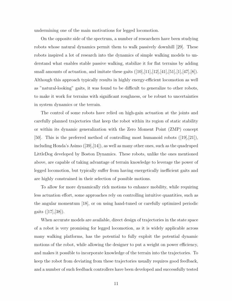
wheeled robots, as illustrated in Figure 1-1 borrowed from [38]. The figure shows

the legged robot navigating across gaps, up steps, and on steep slopes, which is

not possible for a similar wheeled robot. In addition, the extra degrees of freedom

available to a legged robot allow it to come back from otherwise unrecoverable states.

These advantages are further amplified by the design of human environments, which

are typically made accessible to bipedal humans, and might not always permit wheeled

vehicles. A common, but not the only case, are stairs, which are ubiquitous in modern

architecture.

Despite the advantages in their ability to navigate difficult terrain, legged robots

have seen little practical use, mostly because of increased complexity that requires

more careful design of the robot and the control method. Legged robots are faced

with the challenges of dealing with changing configurations during walking or running

motions, and of having to carry a large number of actuators that are typically used

intermittently and have widely varying loads. Because of these constraints and limits

on how much actuation can be reasonably carried, torque and velocity limits are usu-

ally important constraints for these robots, making the already non-linear dynamics

even more complex to model and control. At every step, a legged robot has to deal

9

Figure 1-1: Advantages of legged over wheeled locomotionFigure borrowed from [38]. Legged robot navigating over gaps, up steps, on steepinclines, and recovering from falls, which is not possible with a similar wheeled robot.

with ground impacts, which are difficult to model, because of their stochastic nature

and dependence on the state of the robot, as well as on the properties of the foot

and the ground it is stepping on. Finally, bipedal robots and quadruped robots using

fast gaits both have to deal with underactuated dynamics, which can’t be controlled

directly and require more careful planning and execution of trajectories.

1.2 State of Legged Locomotion

There have been a number of impressive results in legged locomotion, particularly

on the hardware side, and arguably the most success has been seen in robots that

were carefully designed to generate walking or running motions with simplistic and

intuitive control.

A good example of this are the robots developed in the MIT Leg Lab and later at

Boston Dynamics ([37],[36],[35]). These robots rely on using large amount of actuation

to make them behave like a one-legged hopping robot, which is well understood and

can be effectively controlled with simple techniques. However, these simplifications

rely on a particular design of the robot, are quite power intensive, and typically can’t

use information about external terrain, significantly limiting their robustness and

10

undermining one of the main motivations for legged locomotion.

On the opposite side of the spectrum, a number of researchers have been studying

robots whose natural dynamics permit them to walk passively downhill [29]. These

robots inspired a lot of research into the dynamics of simple walking models to un-

derstand what enables stable passive walking, stabilize it for flat terrains by adding

small amounts of actuation, and imitate these gaits ([10],[11],[12],[41],[51],[1],[47],[8]).

Although this approach typically results in highly energy-efficient locomotion as well

as ”natural-looking” gaits, it was found to be difficult to generalize to other robots,

to make it work for terrains with significant roughness, or be robust to uncertainties

in system dynamics or the terrain.

The control of some robots have relied on high-gain actuation at the joints and

carefully planned trajectories that keep the robot within its region of static stability

or within its dynamic generalization with the Zero Moment Point (ZMP) concept

[50]. This is the preferred method of controlling most humanoid robots ([19],[21]),

including Honda’s Asimo ([39],[14]), as well as many other ones, such as the quadruped

LittleDog developed by Boston Dynamics. These robots, unlike the ones mentioned

above, are capable of taking advantage of terrain knowledge to leverage the power of

legged locomotion, but typically suffer from having energetically inefficient gaits and

are highly constrained in their selection of possible motions.

To allow for more dynamically rich motions to enhance mobility, while requiring

less actuation effort, some approaches rely on controlling intuitive quantities, such as

the angular momentum [18], or on using hand-tuned or carefully optimized periodic

gaits ([17],[38]).

When accurate models are available, direct design of trajectories in the state space

of a robot is very promising for legged locomotion, as it is widely applicable across

many walking platforms, has the potential to fully exploit the potential dynamic

motions of the robot, while allowing the designer to put a weight on power efficiency,

and makes it possible to incorporate knowledge of the terrain into the trajectories. To

keep the robot from deviating from these trajectories usually requires good feedback,

and a number of such feedback controllers have been developed and successfully tested

11

on real robots ([2],[42],[6],[52],[48]). One of these controllers, transverse linearization,

has been recently successfully used to stabilize trajectories for a number of simple

walking models and real robots ([43],[24]). In this work, we apply the idea of trajectory

optimization with transverse linearization to the significantly more challenging task

of generating stable bounding of Boston Dynamic’s LittleDog over rough terrain.

1.3 LittleDog

The ”Learning Locomotion” program [33] was a DARPA project that provided a

number of university research teams with a set of rough terrains and the LittleDog

robot [30], designed for this purpose by Boston Dynamics. The goal of the project

was to plan and navigate over these terrains as quickly as possible with LittleDog in

the environment of good off-board position estimation and perfect terrain knowledge.

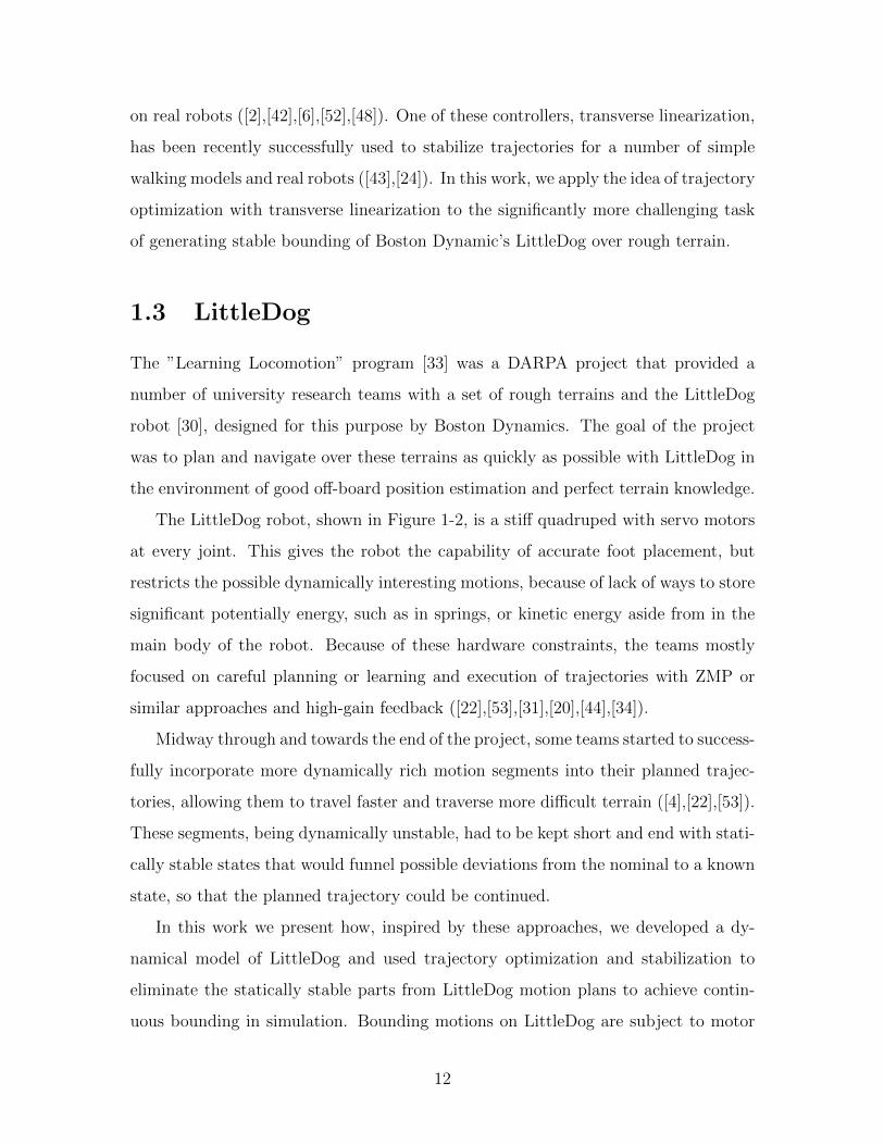
The LittleDog robot, shown in Figure 1-2, is a stiff quadruped with servo motors

at every joint. This gives the robot the capability of accurate foot placement, but

restricts the possible dynamically interesting motions, because of lack of ways to store

significant potentially energy, such as in springs, or kinetic energy aside from in the

main body of the robot. Because of these hardware constraints, the teams mostly

focused on careful planning or learning and execution of trajectories with ZMP or

similar approaches and high-gain feedback ([22],[53],[31],[20],[44],[34]).

Midway through and towards the end of the project, some teams started to success-

fully incorporate more dynamically rich motion segments into their planned trajec-

tories, allowing them to travel faster and traverse more difficult terrain ([4],[22],[53]).

These segments, being dynamically unstable, had to be kept short and end with stati-

cally stable states that would funnel possible deviations from the nominal to a known

state, so that the planned trajectory could be continued.

In this work we present how, inspired by these approaches, we developed a dy-

namical model of LittleDog and used trajectory optimization and stabilization to

eliminate the statically stable parts from LittleDog motion plans to achieve contin-

uous bounding in simulation. Bounding motions on LittleDog are subject to motor

12

Figure 1-2: The LittleDog robot on a rock terrainLittleDog is a stiff quadruped robot developed by Boston Dynamics.

13

saturations, impacts, and underactuated dynamics, capturing many of the difficulties

of legged locomotion, making these methods applicable across many walking robots.

1.4 Contributions

In this work, we develop and identify an accurate dynamical model of the LittleDog

robot that combines simple models of the robot’s motors and links, as well as a novel

ground interaction model. Using the model, we construct an estimator for LittleDog,

based on the Extended Kalman Filter, but modified to carefully correct for delays in

the sensing. We discuss the effects of having large control time steps on transverse

linearization and then construct an algorithm for applying LQR with transverse lin-

earization in this context. We then demonstrate successful robust bounding of the

LittleDog robot across a wide variety of terrains in simulation.

The work is organized as follows. In Chapter 2 we provide a more detailed overview

of our approach for stabilizing LittleDog bounding. Chapter 3 presents the planar

dynamic model of the robot and its identification procedure. Chapter 4 goes into

detail about the state estimator, while Chapter 5 goes into detail about the feedback

controller. Chapter 6 presents our result of stable bounding in simulation, the issues

arising from feedback between the control and estimation algorithms and discusses our

attempts to make the approach work on the real robot. Finally, Chapter 7 provides

a summary of this work and discusses potential future improvements.

14

Chapter 2

Framework

Figure 2-1 shows the approach taken in this work to achieve bounding locomotion of

LittleDog over rough terrain.

In general, the task of a locomotion algorithm is to move the robot from a start

position to the desired goal position by computing an appropriate set of motor com-

mands based on the sensor readings. To keep the dimensionality of the state space as

low as possible, making the task more tractable, while still allowing some capability

for interesting dynamical motions, we chose to restrict the LittleDog dynamics to the

sagittal plane. This was accomplished by constraining the front pair as well as the

back pair of legs to move in unison and making the height of the terrain invariant with

respect to the direction orthogonal to LittleDog’s plane of motion. The constraint

makes a bounding gait the only practical method of navigating for the robot, since,

unless it drags its feet for the whole distance, it is forced to alternate between lifting

the front and back legs.

The number of possible dynamical states of the robot is large, its motions are

sensitive to deviations in the states and inputs as well as to external disturbances,

the sensor readings are subject to noise, and it is not in general possible to bring the

robot into a desired dynamical state directly. For that reason, directly learning the

motor commands that will robustly take the robot from the start to the goal is com-

putationally prohibitive. Even if it was accomplished, a small change to the robot’s

dynamics or the terrain would, in general, require the commands to be relearned from

15

Figure 2-1: LittleDog bounding control frameworkThe planning algorithm creates a feasible trajectory from the start to the goal statesfor a given terrain. A set of gains is computed for the trajectory and used in areal-time control and estimation feedback loop to stabilize the robot. The planning,estimation, and control portions rely on an accurate dynamical model of LittleDog.

16

scratch. The alternative to directly learning the commands is model-based control.

We have developed a physics-based model that allows us to predict the response of

LittleDog to a given set of commands, making it possible to develop a control policy

without directly exploring all possible configurations on the physical robot. As seen

in Figure 2-1, most parts of the bounding algorithm rely on the model’s predictions.

We use a model based on multiple rigid-body links, with motor dynamics at the joints

and a novel ground contact model. Chapter 3 goes into detail about the structure of

the model and the methods used to identify its parameters.

To further simplify the bounding task, we employ a standard control systems

approach of separating the feedback control and estimation problems. The estimation

algorithm computes a state estimate based on the previous estimate, sensor readings,

and a model of the robot’s sensors and passes it to the feedback control algorithm, so

the latter can be designed in the state space of the model instead of the space of all

possible stochastic sensor histories. This simplification tends to work well as long as

errors in the state estimate are sufficiently small to not destabilize the overall system.

For state estimation we use an Extended Kalman Filter with a few alterations to

accommodate for time delays. A detailed description of LittleDog sensors and the

relevant time delays, the EKF implementation, and an evaluation of its performance

are given in Chapter 4.

Even with the simplifications listed above, for a complex dynamical system such

as LittleDog it is not practical (or even feasible, since it is impossible to recover from

certain states) to produce a valid control policy for every possible state. Luckily, this is

not necessary when only a small fraction of the state space is expected to be visited. In

this work, we use a common approach of computing a feasible trajectory of states from

the starting state to an end state inside the goal region and a set of motor commands

that generate the trajectory. This is accomplished by the RG-RRT algorithm ([46],

[45]), which was able to plan trajectories over a wide variety of terrains. The RG-RRT

algorithm starts from the initial state and constructs a tree that sparsely explores the

reachable states, while pruning out states that result in collisions or don’t meet certain

heuristics. The tree is constructed by randomly sampling motion primitives for motor

17

commands and using the LittleDog model presented in Chapter 3 to compute the state

transitions for these primitives. The output of the planning algorithm is a trajectory

of states and a set of motor commands that, when executed on the robot starting

from the initial state, will cause it to go through the states of the trajectory and end

up at the goal state.

However, when executed on a real physical system, because of stochastic dis-

turbances and imperfections in the modeling, the actual trajectory might diverge

arbitrarily far from the theoretical one. Model Predictive Control [28] solves this

by computing a new trajectory at every timestep, but this is, in general, computa-

tionally expensive and might not be possible to do in real time. For example, for

LittleDog, computing a feasible trajectory to the goal with RG-RRT takes on the

order of 10 minutes. A more efficient approach is to compute, for states close to the

original trajectory, an adjustment to the motor commands to keep the system near

the original path. If the controller can effectively deal with the perturbations, the

system will remain near the trajectory and will eventually reach a region close to the

goal, as desired. We accomplish this by applying transverse linearization techniques

to the trajectories, as explained in Chapter 5. This is done by re-parametrizing the

trajectories, constructing a new coordinate system that is transverse to the dynamics,

and controlling the transverse dynamics using a gain-scheduling controller based on

the LQR cost function.

18

Chapter 3

Model

An essential component of any model-based planning approach is a sufficiently accu-

rate identification of the system dynamics. Obtaining an accurate dynamic model for

LittleDog is challenging due to subtleties in the ground interactions and the domi-

nant effects of motor saturations and transmission dynamics. These effects are more

pronounced in bounding gaits than in walking gaits, due to the increased magnitude

of ground reaction forces at impact and the perpetual saturations of the motor; as

a result, we required a more detailed model. In this section, we describe our system

identification procedure and results.

The LittleDog robot has 12 actuators (two in each hip, one in each knee) and a

total of 22 essential degrees of freedom (six for the body, three rotational joints in

each leg, and one prismatic spring in each leg). By assuming that the leg springs are

over-damped, yielding first-order dynamics, we arrive at a 40 dimensional state space

(18× 2 + 4). However, to keep the model as simple (low-dimensional) as possible, we

approximate the dynamics of the robot using a planar 5-link serial rigid-body chain

model, with revolute joints connecting the links, and a free base joint, as shown in

Figure 3-1. The planar model assumes that the back legs move together as one and

the front legs move together as one. Each leg has a single hip joint, connecting the leg

to the main body, and a knee joint. The foot of the real robot is a rubber-coated ball

that connects to the shin through a small spring (force sensor), which is constrained

to move along the axis of the shin. The spring is stiff, heavily damped, and has a

19

limited travel range, so it is not considered when computing the kinematics of the

robot, but is important for computing the ground forces. In addition, to reduce the

state space, only the length of the shin spring is considered. This topic is discussed

in detail as part of the ground contact model.

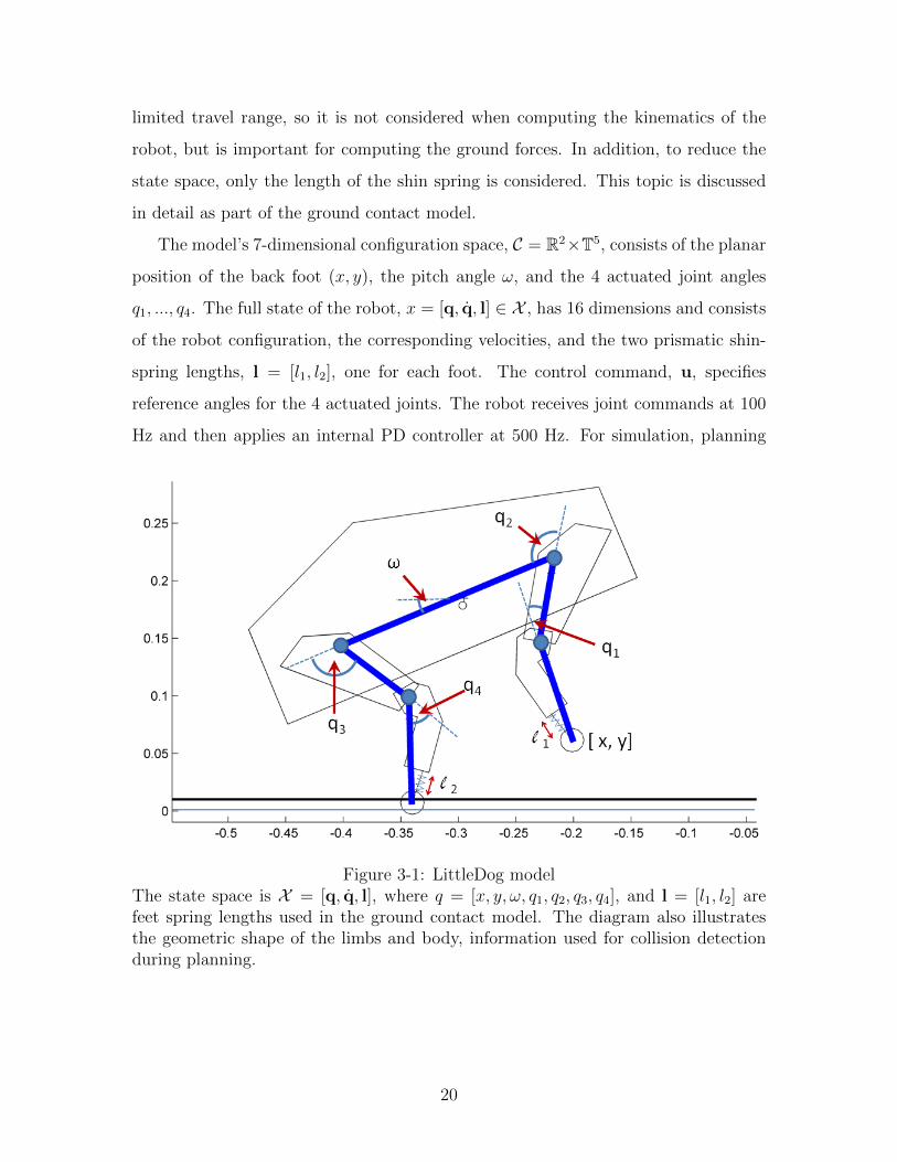
The model’s 7-dimensional configuration space, C = R2×T5, consists of the planar

position of the back foot (x, y), the pitch angle ω, and the 4 actuated joint angles

q1, ..., q4. The full state of the robot, x = [q, q, l] ∈ X , has 16 dimensions and consists

of the robot configuration, the corresponding velocities, and the two prismatic shin-

spring lengths, l = [l1, l2], one for each foot. The control command, u, specifies

reference angles for the 4 actuated joints. The robot receives joint commands at 100

Hz and then applies an internal PD controller at 500 Hz. For simulation, planning

Figure 3-1: LittleDog modelThe state space is X = [q, q, l], where q = [x, y, ω, q1, q2, q3, q4], and l = [l1, l2] arefeet spring lengths used in the ground contact model. The diagram also illustratesthe geometric shape of the limbs and body, information used for collision detectionduring planning.

20

and control purposes, the dynamics are defined as

x[n+ 1] = f(x[n],u[n]), (3.0)

where x[n+1] is the state at t[n+1], x[n] is the state at t[n], and u[n] is the actuated

joint position command applied during the time interval between t[n] and t[n + 1].

We will sometimes refer to the control time step, ∆T = t[n+ 1]− t[n] = 0.01 seconds.

A fixed-step 4th order Runge-Kutta integration of the continuous Euler-Lagrange

dynamics model is used to compute the state update.

A self-contained motor model is used to describe the movement of the actuated

joints. Motions of these joints are prescribed in the 5-link system, so that as the

dynamics are integrated forward, joint torques are back-computed, and the joint

trajectory specified by the model is exactly followed. This model is also constrained

so that actuated joints respect bounds placed on angle limits, actuator velocity limits,

and actuator torque limits. In addition, forces computed from a ground contact model

are applied to the 5-link chain when the feet are in contact with the ground. The

motor model and ground contact forces are described in more detail below. The

actuated joints are relatively stiff, so the model is most important for predicting the

motion of the unactuated degrees of freedom of the system, in particular the pitch

angle, as well as the horizontal position of the robot.

3.1 Motor Model

The motors on LittleDog have gear ratios of approximately 70 : 1. Because of the high

gear ratio, the internal second-order dynamics of the individual motors dominate in

most cases, and the rigid-body dynamics of a given joint, as well as effects of inertial

coupling and external forces on the robot can be neglected. The combination of the

motor internal dynamics with the PD controller with fixed PD gains can be accurately

modeled as a linear second-order system:

qi = −bqi + k(ui − qi), (3.0)

21

where qi is the acceleration applied to the ith joint, given the state variables [qi, qi] and

the desired position ui. To account for the physical limitations of actual motors, the

model includes hard saturations on the velocity and acceleration of the joints. The

velocity limits, in particular, have a large effect on the joint dynamics in practice.

Each of the 4 actuated joints is assumed to be controlled by a single motor, with

both of the knee joints having one pair of identical motors, and the hip joints having

a different pair of identical motors (the real robot has a differential in the hip, but not

the knee). Because of this, two separate motor parameter sets: b, k, vlim, alim are

used, one for the knees, and one for the hips. The velocity limits of the joints, vlim,

are the result of counter EMF in the DC motors. When the acceleration limits, alim

are reached, the response is non-smooth and results in the motors stuttering, which

is not practical to model. This suggests that alim are a result of current failsafes

in LittleDog’s electronics, but it is not possible to confirm that because of lack of

access to the robot’s internals. In agreement with the guess, alim depends on the

amount of load on the joints of the robot, but is modeled to be constant for simplicty.

Increasing the external power supply voltage increases alim and reduces the stuttering,

so for all experiments the voltage was set to 20V , which is the maximum allowed value

according to LittleDog specifications.

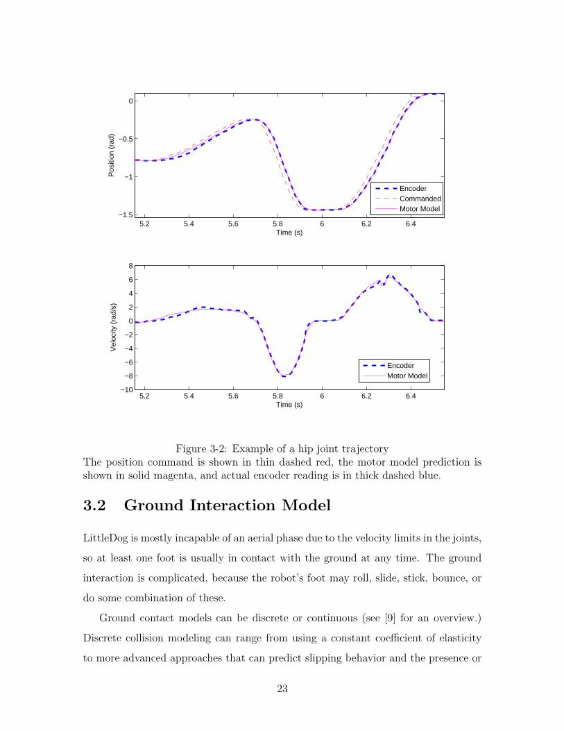
Figure 3-2 shows a typical fit of the motor model to motor encoder readings,

collected from a number of bounding gaits. The fits are consistent across the different

joints of the robot and across different LittleDog robots, but depend on the gains of

the PD controller at each of the joints. As seen from the figure, the motor model does

well in tracking the actual joint position and velocity. Under large dynamic loads,

such as when the hip is lifting and accelerating the whole robot body at the beginning

of a bound, the model might slightly lead the actual joint readings. This can be seen

in Figure 3-2 (top) at 5.4 s. For the knee joint and for less aggressive trajectories

with the hip, the separation is not significant. Additionally, note that backlash in the

joints is not modeled. The joint encoders are located on the motors rather than the

joint axes, which makes it very difficult to measure and model backlash.

22

5.2 5.4 5.6 5.8 6 6.2 6.4−1.5

−1

−0.5

0

Time (s)

Pos

ition

(ra

d)

EncoderCommandedMotor Model

5.2 5.4 5.6 5.8 6 6.2 6.4−10

−8

−6

−4

−2

0

2

4

6

8

Time (s)

Vel

ocity

(ra

d/s)

EncoderMotor Model

Figure 3-2: Example of a hip joint trajectoryThe position command is shown in thin dashed red, the motor model prediction isshown in solid magenta, and actual encoder reading is in thick dashed blue.

3.2 Ground Interaction Model

LittleDog is mostly incapable of an aerial phase due to the velocity limits in the joints,

so at least one foot is usually in contact with the ground at any time. The ground

interaction is complicated, because the robot’s foot may roll, slide, stick, bounce, or

do some combination of these.

Ground contact models can be discrete or continuous (see [9] for an overview.)

Discrete collision modeling can range from using a constant coefficient of elasticity

to more advanced approaches that can predict slipping behavior and the presence or

23

absence of bounce [3]. Discrete modeling is advantageous because of its simplicity,

but is not well suited for LittleDog, because it assumes an instantaneous change in

momentum, whereas on the robot compression of shin springs extends the collision

duration to a time-scale comparable with the rest of LittleDog dynamics. Continuous

impact modeling is more suited for LittleDog and can be subdivided into modeling

the forces normal and tangential to the surface. The ground contact model presented

here carefully computes the interaction of LittleDog feet with rough terrain, allowing

it to predict shin-spring displacement, foot roll, foot slip, compliance and energy

dissipation during ground collision, and bounce when too little energy is dissipated.

A continuous, elastic ground interaction model is used, where the foot of the

robot is considered as a ball, and at each point in time the forces acting on the

foot are computed. The ground plane is assumed to be compressible, with a stiff

nonlinear spring damper normal to the ground that pushes the foot out of the terrain.

A tangential friction force, based on a nonlinear model of Coulomb friction is also

assumed. The normal and friction forces are balanced with the force of the shin spring

at the bottom of the robot’s leg. The rate of change of the shin spring, l, is computed

by the force balancing and used to update the shin-spring length, l, which is a part

of the state space. The resulting normal and friction forces are applied to the 5-link

model.

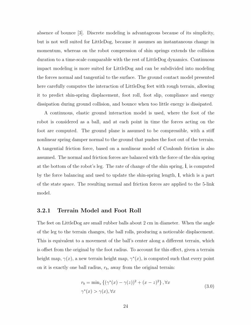
3.2.1 Terrain Model and Foot Roll

The feet on LittleDog are small rubber balls about 2 cm in diameter. When the angle

of the leg to the terrain changes, the ball rolls, producing a noticeable displacement.

This is equivalent to a movement of the ball’s center along a different terrain, which

is offset from the original by the foot radius. To account for this effect, given a terrain

height map, γ(x), a new terrain height map, γ∗(x), is computed such that every point

on it is exactly one ball radius, rb, away from the original terrain:

rb = minz (γ∗(x)− γ(z))2 + (x− z)2 ,∀x

γ∗(x) > γ(x),∀x(3.0)

24

Both height maps can be seen in Figure 3-1, where the bottom light blue horizontal

line is γ(x), the original terrain, and the black line above it is γ∗(x), the terrain

computed by Equation (3.2.1). In this case, γ∗(x) = γ(x) + rb, but this is not

generally true for non-flat terrain.

When a LittleDog foot rolls, the velocity of the foot center is different from the

velocity at the ground contact by rbθ, where θ is the absolute angular velocity of the

foot. The new height map and the adjustment to ground contact velocity completely

capture the foot roll behavior.

All ground contact computations use the new height map, γ∗(x), referred to as

‘the terrain’ below. A function for the slope of the terrain, α(x), is computed from

γ∗(x).

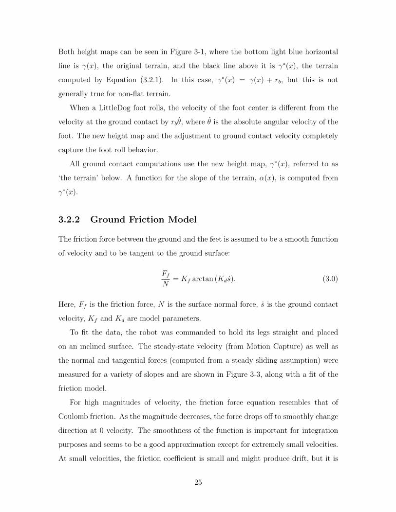
3.2.2 Ground Friction Model

The friction force between the ground and the feet is assumed to be a smooth function

of velocity and to be tangent to the ground surface:

FfN

= Kf arctan (Kds). (3.0)

Here, Ff is the friction force, N is the surface normal force, s is the ground contact

velocity, Kf and Kd are model parameters.

To fit the data, the robot was commanded to hold its legs straight and placed

on an inclined surface. The steady-state velocity (from Motion Capture) as well as

the normal and tangential forces (computed from a steady sliding assumption) were

measured for a variety of slopes and are shown in Figure 3-3, along with a fit of the

friction model.

For high magnitudes of velocity, the friction force equation resembles that of

Coulomb friction. As the magnitude decreases, the force drops off to smoothly change

direction at 0 velocity. The smoothness of the function is important for integration

purposes and seems to be a good approximation except for extremely small velocities.

At small velocities, the friction coefficient is small and might produce drift, but it is

25

−0.1 −0.05 0 0.05 0.1 0.15−0.8

−0.6

−0.4

−0.2

0

0.2

0.4

0.6

0.8

Ground Contact Velocity (m/s)

Ff/N

Figure 3-3: Friction coefficient fitFriction coefficient versus steady state velocity on an inclined plane.

negligible in typical timescales of a simulation run (less than 1 minute). An arc-

tangent was selected for the functional form because it fits the available data well,

but other sigmoids could be used.

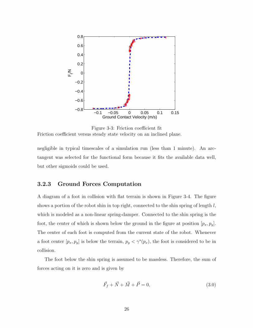
3.2.3 Ground Forces Computation

A diagram of a foot in collision with flat terrain is shown in Figure 3-4. The figure

shows a portion of the robot shin in top right, connected to the shin spring of length l,

which is modeled as a non-linear spring-damper. Connected to the shin spring is the

foot, the center of which is shown below the ground in the figure at position [px, py].

The center of each foot is computed from the current state of the robot. Whenever

a foot center [px, py] is below the terrain, py < γ∗(px), the foot is considered to be in

collision.

The foot below the shin spring is assumed to be massless. Therefore, the sum of

forces acting on it is zero and is given by

~Ff + ~N + ~M + ~P = 0, (3.0)

26

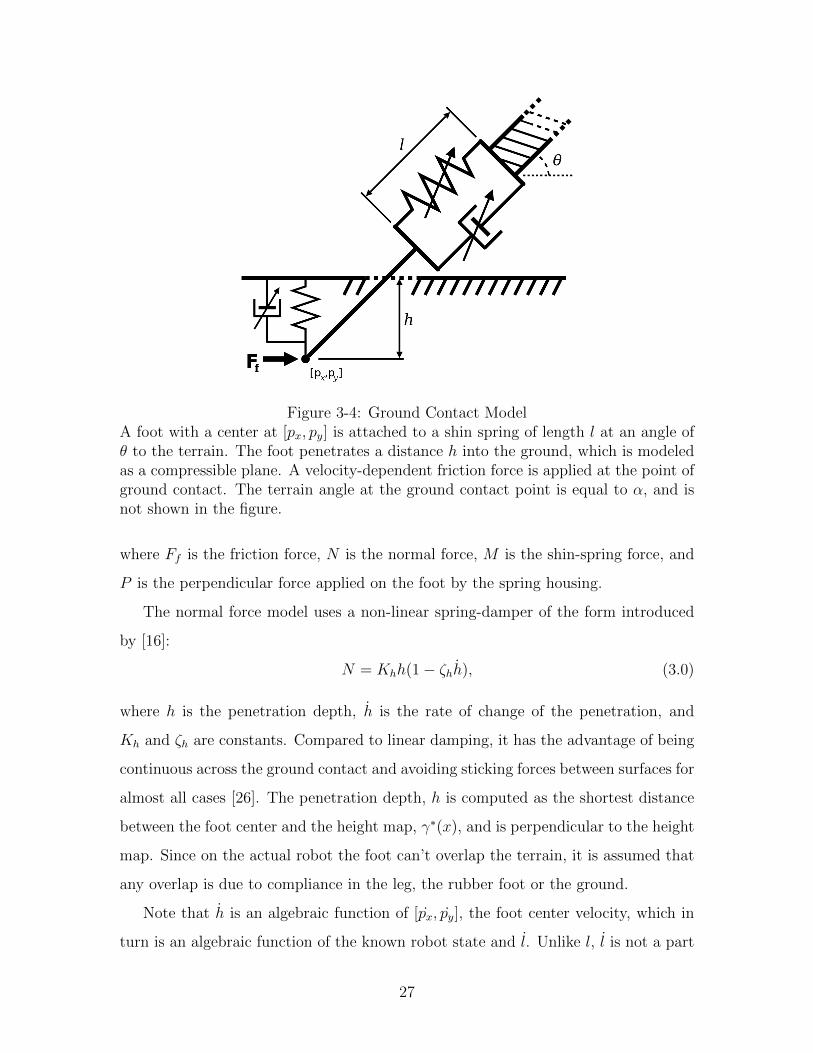
Figure 3-4: Ground Contact ModelA foot with a center at [px, py] is attached to a shin spring of length l at an angle ofθ to the terrain. The foot penetrates a distance h into the ground, which is modeledas a compressible plane. A velocity-dependent friction force is applied at the point ofground contact. The terrain angle at the ground contact point is equal to α, and isnot shown in the figure.

where Ff is the friction force, N is the normal force, M is the shin-spring force, and

P is the perpendicular force applied on the foot by the spring housing.

The normal force model uses a non-linear spring-damper of the form introduced

by [16]:

N = Khh(1− ζhh), (3.0)

where h is the penetration depth, h is the rate of change of the penetration, and

Kh and ζh are constants. Compared to linear damping, it has the advantage of being

continuous across the ground contact and avoiding sticking forces between surfaces for

almost all cases [26]. The penetration depth, h is computed as the shortest distance

between the foot center and the height map, γ∗(x), and is perpendicular to the height

map. Since on the actual robot the foot can’t overlap the terrain, it is assumed that

any overlap is due to compliance in the leg, the rubber foot or the ground.

Note that h is an algebraic function of [px, py], the foot center velocity, which in

turn is an algebraic function of the known robot state and l. Unlike l, l is not a part

27

of the state, so h can’t be computed directly. The normal force is affine in l, so, for

a robot in state x, Equation (3.2.3) can be rewritten as

N = Nx(x) +Nl(x)l, (3.0)

where Nx(x) an Nl(x) are non-linear functions of the state.

The actual shin spring on the robot is limited in its range of travel. During a

bounding motion, it is typical for the spring to reach the limits of motion, where it

hits a hard stop. The spring is modeled as linear in its normal range and to have

a hard collision at the travel limits of the same functional form as the normal force.

Assuming a rest length of l0, the displacement from rest is δl = l − l0, and the range

of travel for δl is between 0 and lmax, the force is given by

M =

Ksδl + bsl +Kcδl(1 + ζl l), δl < 0

Ksδl + bsl, 0 ≤ δl < lmax

Ksδl + bsl +Kc(δl − lmax)(1− ζl l), lmax ≤ δl

(3.0)

where Ks and Kc Ks are stiffness parameters, bs and ζl are damping parameters.

Similarly to the normal force, the spring force is affine in l and can be written as

M = Mx(x) +Ml(x)l (3.0)

for some nonlinear functions of the state Mx(x) and Ml(x).

The friction force is given by Equation (3.2.2), where s is the velocity of the foot

center along the height map γ∗(x) and can be computed from the state of the robot

x, the slope of the terrain at the ground contact α, and l.

The force applied to the foot by the spring housing, P , is unknown, but can be

eliminated from the force balance by only considering the component of Equation

(3.2.3) that is orthogonal to P . Noting that M ⊥ P , Ff ⊥ N , the angle between the

28

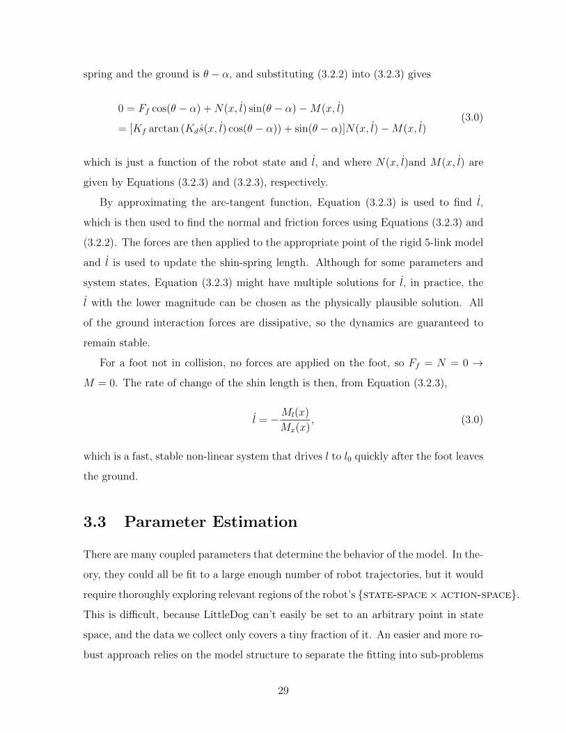
spring and the ground is θ − α, and substituting (3.2.2) into (3.2.3) gives

0 = Ff cos(θ − α) +N(x, l) sin(θ − α)−M(x, l)

= [Kf arctan (Kds(x, l) cos(θ − α)) + sin(θ − α)]N(x, l)−M(x, l)(3.0)

which is just a function of the robot state and l, and where N(x, l)and M(x, l) are

given by Equations (3.2.3) and (3.2.3), respectively.

By approximating the arc-tangent function, Equation (3.2.3) is used to find l,

which is then used to find the normal and friction forces using Equations (3.2.3) and

(3.2.2). The forces are then applied to the appropriate point of the rigid 5-link model

and l is used to update the shin-spring length. Although for some parameters and

system states, Equation (3.2.3) might have multiple solutions for l, in practice, the

l with the lower magnitude can be chosen as the physically plausible solution. All

of the ground interaction forces are dissipative, so the dynamics are guaranteed to

remain stable.

For a foot not in collision, no forces are applied on the foot, so Ff = N = 0 →

M = 0. The rate of change of the shin length is then, from Equation (3.2.3),

l = −Ml(x)

Mx(x), (3.0)

which is a fast, stable non-linear system that drives l to l0 quickly after the foot leaves

the ground.

3.3 Parameter Estimation

There are many coupled parameters that determine the behavior of the model. In the-

ory, they could all be fit to a large enough number of robot trajectories, but it would

require thoroughly exploring relevant regions of the robot’s state-space× action-space.

This is difficult, because LittleDog can’t easily be set to an arbitrary point in state

space, and the data we collect only covers a tiny fraction of it. An easier and more ro-

bust approach relies on the model structure to separate the fitting into sub-problems

29

and to identify each piece separately. The full dynamical model of the robot consists

of the 5-link rigid body, the motor model, and the ground force model. A series of

experiments, described below, and a variety of short bounding trajectories were used

to fit the model parameters to actual robot dynamics by minimizing quadratic cost

functions over simulation error. All of the fits were computed with nonlinear function

optimization (using MATLAB’s fminsearch).

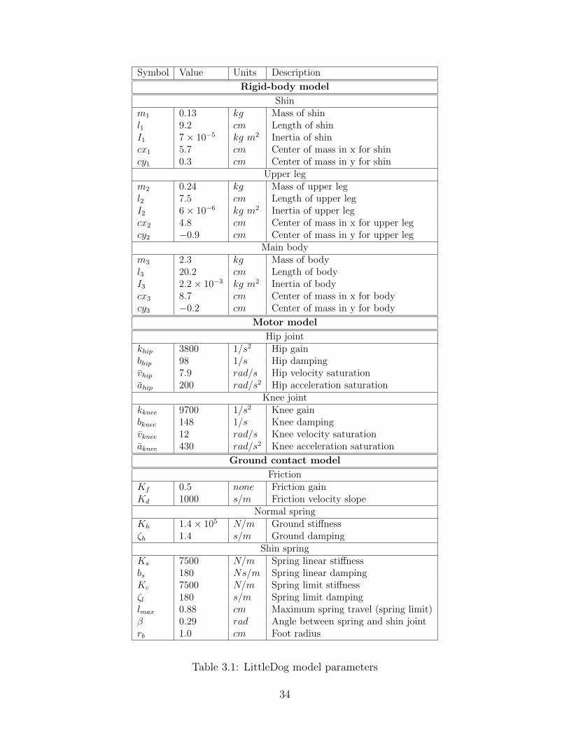
In total, 34 parameters were measured or fit for the model. Table 3.1 lists the

parameters and their values. In the table, the length of the shin is given from the

knee joint to the foot center, assuming full extension of the shin spring. Centers of

masses are given in the reference frames of their links, with x pointing along its link

and y perpendicular to it in a right-handed convention. The origin of the back shin is

at the back foot and x points toward the knee joint, the origin of the back upper leg

is at the knee joint and its x points toward the hip joint, and the origin of the body

is at the back hip joint, with its x pointing toward the front hip joint. The front links

have mirror symmetry with the back legs.

The motor model was assumed to be independent of the other parameters and fit

to real joint trajectory data. The fit accurately predicts the behavior of the joints,

as seen in Figure 3-2, which shows the model performance on a different trajectory.

The friction coefficients in the ground force model were fit to steady-state sliding as

described in section 3.2.2. The rest of the ground contact model was identified by

commanding the robot to hold its legs straight down, parallel to each other, drop-

ping it vertically onto flat terrain, and fitting the parameters to the resulting body

trajectory, measured with Motion Capture. The total mass of the robot, the lengths

of each link, and the maximum shin spring travel were measured directly.

The remaining parameters, including inertias of the links, the mass distribution

between the links, and center of mass locations, were fit to a large number of short

bounding trajectories. The cost function for the fit was a quadratic form on the

distance between actual and simulated feet positions, which captures the effect of the

3 unactuated variables (x, y, and body pitch), neglecting the unactuated shin springs

that are not considered to be a part of the configuration.

30

For the rigid body model, the parameters are heavily coupled and some of the

individual values might not be accurate. This is true of the inertias and to some

degree of the centers of masses. Because the planar model lumps two LittleDog legs

into a single leg, the leg masses and inertias, as well as some of the stiffnesses and

damping values, are twice as large as their physical counterparts for a single leg.

3.3.1 Model Performance

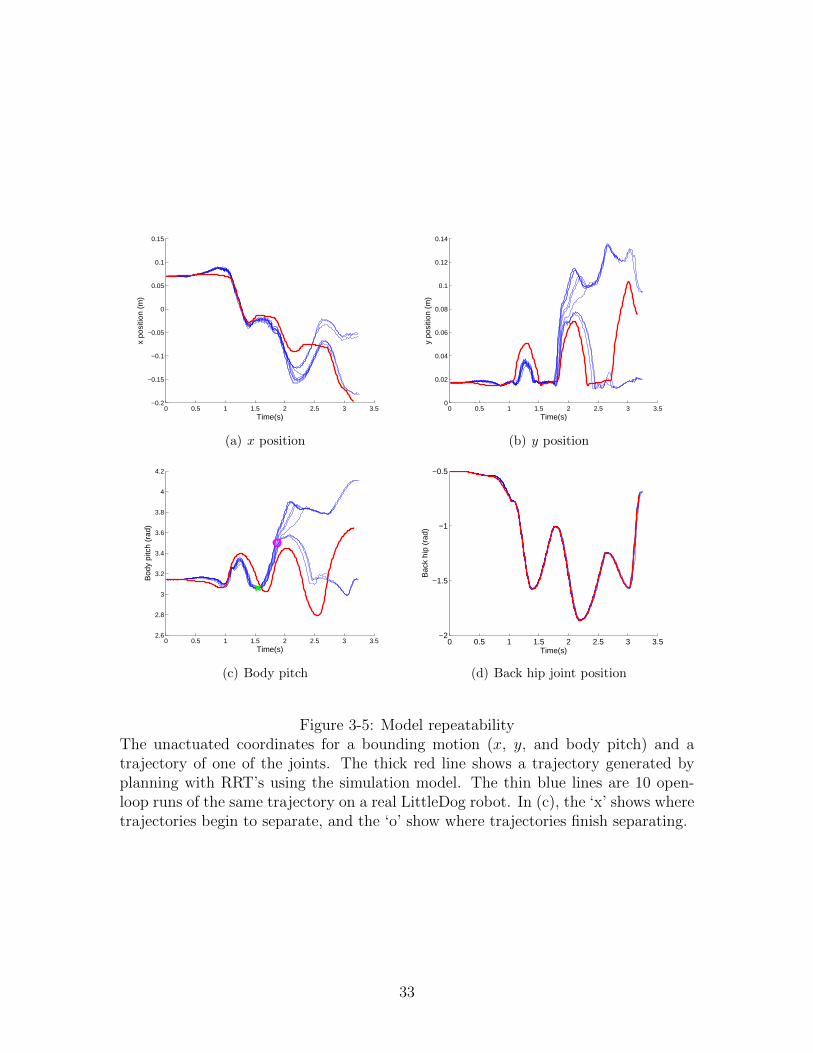
Figure 3-5 shows a comparison of a bounding trajectory in simulation versus 10

runs of the same command executed on the real robot. The simulated trajectory

was generated using the RG-RRT planning algorithm, which used the developed

model. The control input and the starting conditions for all open-loop trajectories in

the figure were identical, and these trajectories were not used for fitting the model

parameters.

Three of the four plots are of an unactuated coordinate (x, y, and body pitch),

the fourth one is of the back hip, an actuated joint. The figure emphasizes the

difference between directly actuated, position controlled joints compared to unstable

and unactuated degrees of freedom. While the motor model tracks the joint positions

almost perfectly, even through collisions with the ground, the unactuated coordinates

of the open-loop trajectories diverge from each other in less than 2 seconds. Right

after completing the first bounding motion, at about 1.5 s, the trajectories separate

as LittleDog is lifting its body on the back feet. At about 1.9 s, in half of the cases the

robot falls forward and goes through a second bounding motion, while in the rest of

the cases it falls backward and can’t continue to bound. The horizontal position and

body pitch coordinates are both highly unstable and unactuated, making it difficult

to stabilize them. The control problem is examined in more detail later in this paper.

The most significant unmodeled dynamics in LittleDog include backlash, stiction

in the shin spring, and more complex friction dynamics. For example, even though the

friction model fits well to steady-state sliding of LittleDog, experiments on the robot

show that during a bounding motion there are high-frequency dynamics induced in

the legs that reduce the effective ground friction coefficient. Also, the assumption of

31

linearity in the normal force in Coulomb friction does not always hold for LittleDog

feet. Modeling these effects is possible, but would involve adding a large number

of additional states with nonlinear high-frequency dynamics to the model, making

it much harder to implement and less practical overall. In addition, the new states

would not be directly observable using currently available sensors, so identifying the

related parameters and initializing the states for simulation would be difficult.

In general, for a complex unstable dynamical system such as LittleDog, some

unmodeled effects will always remain no matter how detailed the model gets. Instead

of capturing all of the effects, the model approximates the overall behavior of the

system, as seen from Figure 3-5. We believe that this model is sufficiently accurate to

generate relevant motion plans in simulation which can be stabilized using feedback

on the real robot.

32

0 0.5 1 1.5 2 2.5 3 3.5−0.2

−0.15

−0.1

−0.05

0

0.05

0.1

0.15

Time(s)

x po

sitio

n (m

)

(a) x position

0 0.5 1 1.5 2 2.5 3 3.50

0.02

0.04

0.06

0.08

0.1

0.12

0.14

Time(s)y

posi

tion

(m)

(b) y position

0 0.5 1 1.5 2 2.5 3 3.52.6

2.8

3

3.2

3.4

3.6

3.8

4

4.2

Time(s)

Bod

y pi

tch

(rad

)

(c) Body pitch

0 0.5 1 1.5 2 2.5 3 3.5−2

−1.5

−1

−0.5

Time(s)

Bac

k hi

p (r

ad)

(d) Back hip joint position

Figure 3-5: Model repeatabilityThe unactuated coordinates for a bounding motion (x, y, and body pitch) and atrajectory of one of the joints. The thick red line shows a trajectory generated byplanning with RRT’s using the simulation model. The thin blue lines are 10 open-loop runs of the same trajectory on a real LittleDog robot. In (c), the ‘x’ shows wheretrajectories begin to separate, and the ‘o’ show where trajectories finish separating.

33

Symbol Value Units Description

Rigid-body model

Shinm1 0.13 kg Mass of shinl1 9.2 cm Length of shinI1 7× 10−5 kg m2 Inertia of shincx1 5.7 cm Center of mass in x for shincy1 0.3 cm Center of mass in y for shin

Upper legm2 0.24 kg Mass of upper legl2 7.5 cm Length of upper legI2 6× 10−6 kg m2 Inertia of upper legcx2 4.8 cm Center of mass in x for upper legcy2 −0.9 cm Center of mass in y for upper leg

Main bodym3 2.3 kg Mass of bodyl3 20.2 cm Length of bodyI3 2.2× 10−3 kg m2 Inertia of bodycx3 8.7 cm Center of mass in x for bodycy3 −0.2 cm Center of mass in y for body

Motor model

Hip jointkhip 3800 1/s2 Hip gainbhip 98 1/s Hip dampingvhip 7.9 rad/s Hip velocity saturationahip 200 rad/s2 Hip acceleration saturation

Knee jointkknee 9700 1/s2 Knee gainbknee 148 1/s Knee dampingvknee 12 rad/s Knee velocity saturationaknee 430 rad/s2 Knee acceleration saturation

Ground contact model

FrictionKf 0.5 none Friction gainKd 1000 s/m Friction velocity slope

Normal springKh 1.4× 105 N/m Ground stiffnessζh 1.4 s/m Ground damping

Shin springKs 7500 N/m Spring linear stiffnessbs 180 Ns/m Spring linear dampingKc 7500 N/m Spring limit stiffnessζl 180 s/m Spring limit dampinglmax 0.88 cm Maximum spring travel (spring limit)β 0.29 rad Angle between spring and shin jointrb 1.0 cm Foot radius

Table 3.1: LittleDog model parameters

34

Chapter 4

State Estimation

The purpose of the state estimation algorithm is to use the available sensors to create

an accurate estimate of LittleDog’s state, with the goal of making the combination

of the estimator and the robot behave similarly to the idealized model developed in

Chapter 3. This involves using the robot’s model to eliminate the noise in the sen-

sors, compensate for sensor delays, and estimate states that are not instantaneously

observable and need to be derived from sensor readings across multiple time steps.

An accurate estimate of the current state allows the use of full state feedback in the

controller.

4.1 LittleDog Sensor and Control Environment

As shown in Figure 4-1, the LittleDog robot is equipped with a number of sensors

to help estimate the state of the robot. The joints contain encoders mounted on the

shafts of the motors, giving a low-noise reading of the motor positions, but making any

effects of backlash unobservable. An on-board IMU (Inertial Measurement Unit) uses

a set of gyroscopes and accelerometers to measure linear accelerations and rotational

velocity of the robot. A set of reflective markers secured on the outside of the robot’s

shell allows a motion capture (MOCAP) system to measure the position of the robot.

In addition to these, LittleDog’s feet are equipped with a set of force sensors, but

we opted to not use them in our state estimation approach. These sensors could be

35

used to detect collisions with the ground, but we found that in order to make the

detection reliable we had to set a high threshold, which delays the contact detection.

Detecting collisions by monitoring state estimates is simpler and has worked suffi-

ciently well in this case. Further work in improving the estimator could look into

incorporating force measurements to create better estimates in the region of transi-

tions to and from ground contact and to better detect transitions between modes,

describes later in the text.

The time delay in reading the encoders is limited to communication delays and

is small with respect to the 10ms timestep, so the encoders are assumed to have 0

delay for the purposes of state estimation. Experiments on the robot show that the

IMU has a delay of about 3 time steps, possibly because of low-level filtering in the

sensor. The MOCAP data also shows a delay of approximately 3 time steps, which

arises because of time needed to process the image data and calculate the coordinates

of the reflective markers.

As mentioned in Chapter 3, each of the motors at the joints is controlled by a servo

loop located on board of LittleDog and executed at 500Hz. The gains for the servo

controllers are fixed and the velocity set points are fixed at 0, while the position set

points act as the control inputs for the off-board control algorithm and are referred to

as control inputs or motor commands in this work. The external, or off-board, control

loop is executed at a frequency of a 100Hz and communicates to the robot over IP,

using the Lightweight Communications and Marshalling (LCM) library[15]. The loop

is shown in Figure 2-1 in red and the design of its estimation and control components

is the focus of this work, with other elements such as the model supporting this goal.

Every 10ms, the external control loop gets the latest readings from the encoders

and the IMU on board of the robot, and the MOCAP system off-board. The estimator

uses the new data to update the current state estimate of LittleDog and passes it to

the feedback control algorithm, which then computes a set of motor commands that

are to be sent to the robot. After transmitting the commands to the servo loop, the

external loop goes idle until the next time step. The execution time of the estimation

and control step, including the time spent on communication, adds a small delay to

36

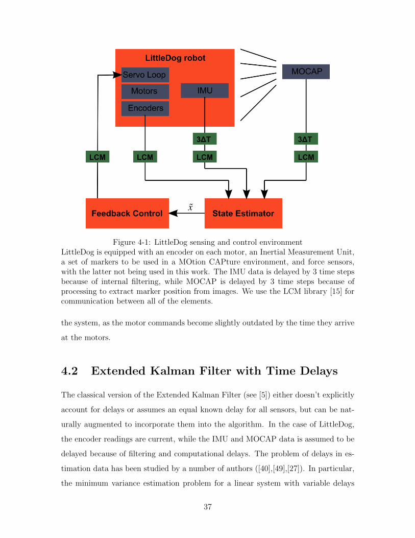
Figure 4-1: LittleDog sensing and control environmentLittleDog is equipped with an encoder on each motor, an Inertial Measurement Unit,a set of markers to be used in a MOtion CAPture environment, and force sensors,with the latter not being used in this work. The IMU data is delayed by 3 time stepsbecause of internal filtering, while MOCAP is delayed by 3 time steps because ofprocessing to extract marker position from images. We use the LCM library [15] forcommunication between all of the elements.

the system, as the motor commands become slightly outdated by the time they arrive

at the motors.

4.2 Extended Kalman Filter with Time Delays

The classical version of the Extended Kalman Filter (see [5]) either doesn’t explicitly

account for delays or assumes an equal known delay for all sensors, but can be nat-

urally augmented to incorporate them into the algorithm. In the case of LittleDog,

the encoder readings are current, while the IMU and MOCAP data is assumed to be

delayed because of filtering and computational delays. The problem of delays in es-

timation data has been studied by a number of authors ([40],[49],[27]). In particular,

the minimum variance estimation problem for a linear system with variable delays

37

for each sensor (with the potential of data loss) has been previously solved, and the

estimator has been demonstrated to be exponentially stable [27]. In this section we

discuss our implementation of the Extended Kalman Filter with time asynchronous

time delays, which can be thought of as a specific case of that problem on the lin-

earization of the system.

Consider a system with discrete dynamics given by

x[n+ 1] = f(x[n], u[n]) + w[n],

where x[n] is the system state at time step n, u[n] is the control input at the time

step, and w[n] is zero mean Gaussian random noise given by

E[w[n]w[l]>] = Q[n]δ(n, l),

where δ(n, l) is the Dirac delta function, and Q[n] ≥ 0 is its covariance. The system

has a set of M sensors described by

zk[n] = hk(x[n− ρk]) + vk[n], k ∈ [1, . . . ,M ],

where zk[n] is the k’th sensor reading, delayed by ρk ∈ N0 time steps, and vk[n] is

zero mean Gaussian random noise such that

Evk[n]vk[l]> = Rk[n]δ(n, l),

Evk[n]vm[l]> = 0 for k 6= m,∀n, l,

Evk[n]wm[l]> = 0 for ∀k, l,m, n,

Rk[n] > 0.

In addition, an estimate of the initial state x[0] = Ex[0] and its covariance P [0] =

E(x[0] − x[0])(x[0] − x[0])> are available. For consistency, assume that zk[n] is

zero for n ≤ ρk. Let ρmax = maxk ρk. Let x[l, n] and P [l, n] represent the minimum

variance estimate of x[l] and its covariance based on the sensor measurements up to

38

timestep n, i.e. zk[m] | k ∈ [1, . . . ,M ],m ∈ [1, . . . , n]. The goal of the estimator is

to compute x[n, n] for each time step n. Note, that when ρk = 0,∀k, the framework

is identical to that of the standard discrete-time Extended Kalman Filter.

The vector of all of the sensor measurements generated by state x[l] and available

at time step n is

Z[l, n] = zk[l + ρk] | l + ρk ≤ n, k ∈ [1, . . . ,M ]. (4.0)

For ρk ≥ 0 and l > n, Z[l, n] = ∅, as expected, since sensor measurements from future

states are not available. Also, after a sufficient time, no new information is received

about the old states, so

Z[l, n] = Z[l,m]

x[l, n] = x[l,m]

P [l, n] = P [l,m]

∀n,m ≥ l + ρmax. (4.0)

Just as in the regular Extended Kalman filter, the estimates are computed on-

line and recursively. For iteration n the vectors Z[l, n], l ∈ [n − ρmax, . . . , n]

are computed using the new sensor readings zk[n], k ∈ [1, . . . ,m] according to

(4.2). Given previously computed P [n − 1 − ρmax, n − 1] = P [n − 1 − ρmax, n] and

x[n − 1 − ρmax, n − 1] = x[n − 1 − ρmax, n] (where the equality follows from (4.2)),

one can get the current state estimate, x[n, n], by recursively applying the prediction

and update steps of the Kalman filter for m ∈ [n− ρmax, . . . , n]:

x∗[m,n] = f(x[m− 1, n], u[m− 1])

P ∗[m,n] = Fm−1,nP [m− 1, n]F>m−1,n +Q[m− 1]

S[m,n] = Gm,nP∗[m,n]G>m,n +R[m]

K[m,n] = P ∗[m,n]G>m,nS−1[m,n]

x[m,n] = x∗[m,n]K[m,n](Z[m,n]−H[m,n])

P [m,n] = (I −K[m,n]Gm,n)P ∗[m,n],

39

where

Fl,n =∂f

∂x(x[l, n])

Hl,n = hk(x[l, n]) | l + ρk ≤ n, k ∈ [1, . . . ,M ]

Gl,n =

∂hk∂x

(x[l, n]) | l + ρk ≤ n, k ∈ [1, . . . ,M ]

,

with the vector Hl,n and matrix Gl,n having the same ordering as Z[l, n], and with

R[m] constructed in a similar way by stacking matrices Rk[m] as blocks on the di-

agonal. For the first few iterations while the filter initializes, when n ≤ ρmax, the

computations are done for m ∈ [1, . . . , n].

Evaluating (4.2) produces the desired estimate x[n, n], as well as x[n−ρmax, n] and

P [n − ρmax, n], which are needed for the next time step of the filter. For LittleDog,

the prediction step (first line in (4.2)) is run for an extra iteration using an estimate

of u[n] to get x[n + 1, n], which is sent as the current state to the controller. The

slight feedforward in estimation helps to compensate for delay in command execution

on the robot.

4.3 Modified Dynamics Model

As described in Chapter 3, the dynamical model of LittleDog has a total of 16 states,

2 of which describe the first-order spring dynamics in the feet of the robot and are

primarily involved in ground interaction modeling. The pair of springs has stiff dy-

namics, significantly faster than the control and sensing rates of the robot, and are

heavily coupled to other states, such as the body position.

Because of difficulty in estimating the spring states and high sensitivity of the

dynamics to their errors, it is best to eliminate the two states from the estimation

and control loop. This is accomplished by using a pinned version of the model for

the estimation and by not using the spring states for feedback.

Using a pinned version makes it necessary to construct 3 separate versions of the

model, corresponding to different modes of the dynamics: pinned at the back foot,

40

pinned at the front foot, and in double support. To construct the version of the model

pinned at the back foot, the ground contact part of the LittleDog model from Chapter

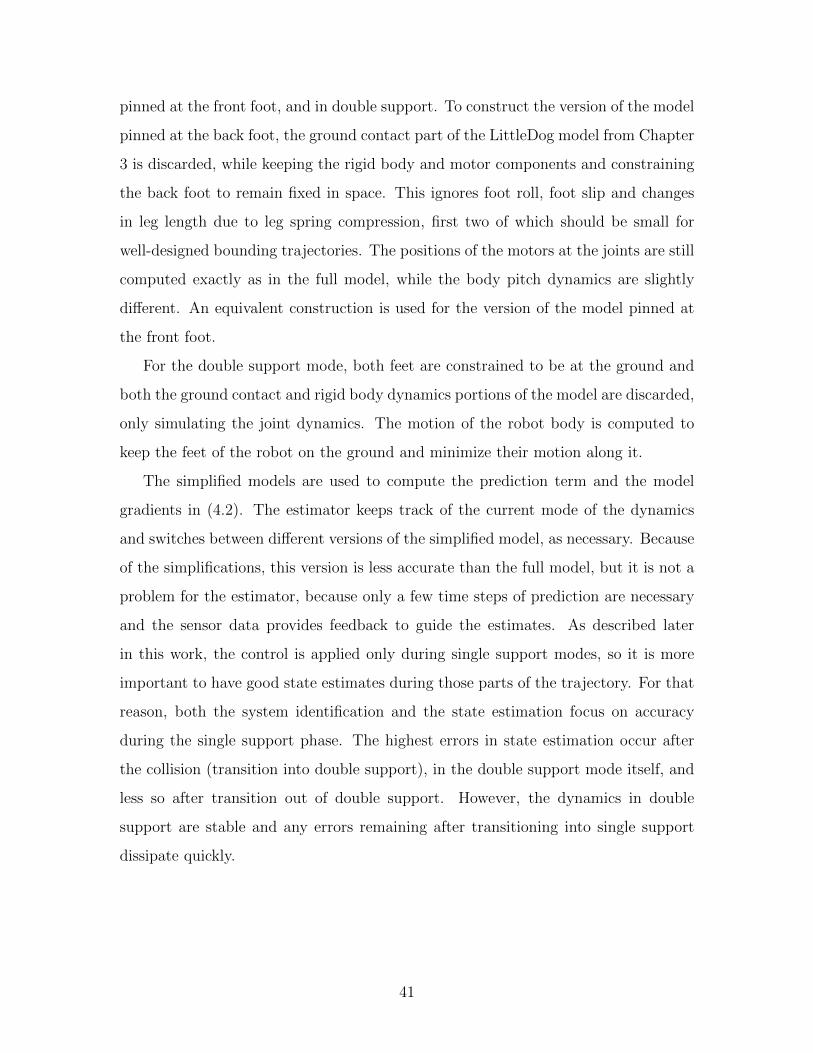
3 is discarded, while keeping the rigid body and motor components and constraining

the back foot to remain fixed in space. This ignores foot roll, foot slip and changes

in leg length due to leg spring compression, first two of which should be small for

well-designed bounding trajectories. The positions of the motors at the joints are still

computed exactly as in the full model, while the body pitch dynamics are slightly

different. An equivalent construction is used for the version of the model pinned at

the front foot.

For the double support mode, both feet are constrained to be at the ground and

both the ground contact and rigid body dynamics portions of the model are discarded,

only simulating the joint dynamics. The motion of the robot body is computed to

keep the feet of the robot on the ground and minimize their motion along it.

The simplified models are used to compute the prediction term and the model

gradients in (4.2). The estimator keeps track of the current mode of the dynamics

and switches between different versions of the simplified model, as necessary. Because

of the simplifications, this version is less accurate than the full model, but it is not a

problem for the estimator, because only a few time steps of prediction are necessary

and the sensor data provides feedback to guide the estimates. As described later

in this work, the control is applied only during single support modes, so it is more

important to have good state estimates during those parts of the trajectory. For that

reason, both the system identification and the state estimation focus on accuracy

during the single support phase. The highest errors in state estimation occur after

the collision (transition into double support), in the double support mode itself, and

less so after transition out of double support. However, the dynamics in double

support are stable and any errors remaining after transitioning into single support

dissipate quickly.

41

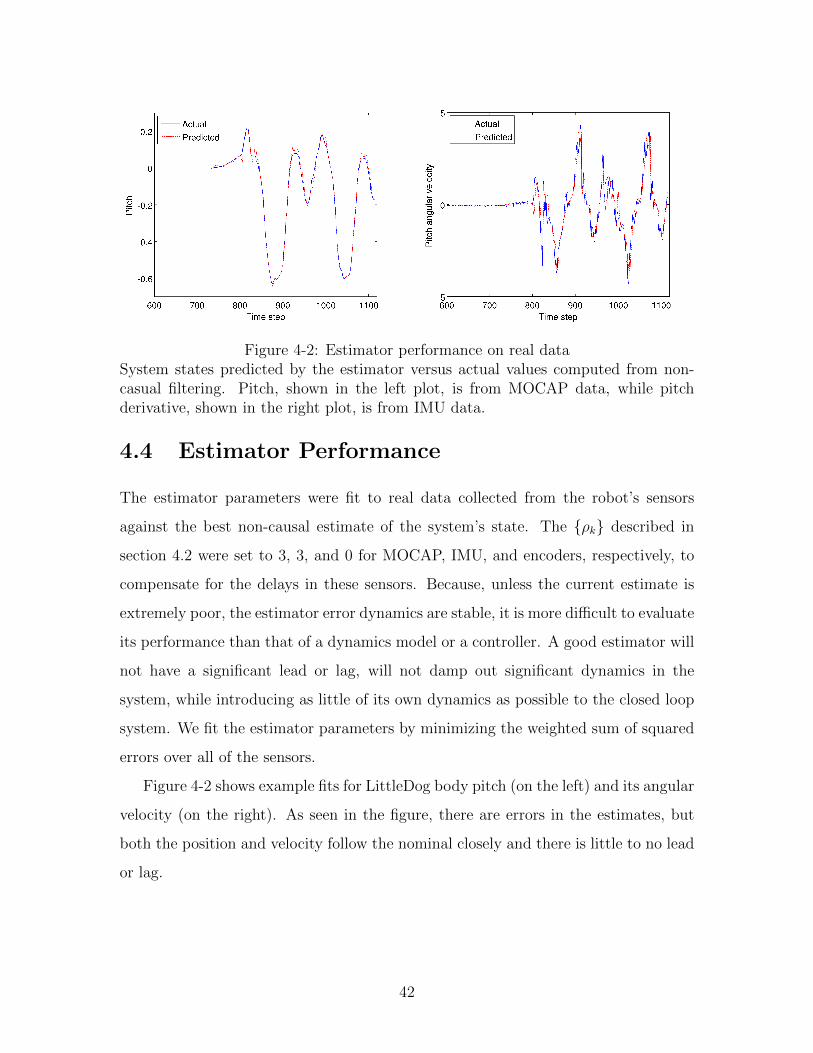
Figure 4-2: Estimator performance on real dataSystem states predicted by the estimator versus actual values computed from non-casual filtering. Pitch, shown in the left plot, is from MOCAP data, while pitchderivative, shown in the right plot, is from IMU data.

4.4 Estimator Performance

The estimator parameters were fit to real data collected from the robot’s sensors

against the best non-causal estimate of the system’s state. The ρk described in

section 4.2 were set to 3, 3, and 0 for MOCAP, IMU, and encoders, respectively, to

compensate for the delays in these sensors. Because, unless the current estimate is

extremely poor, the estimator error dynamics are stable, it is more difficult to evaluate

its performance than that of a dynamics model or a controller. A good estimator will

not have a significant lead or lag, will not damp out significant dynamics in the

system, while introducing as little of its own dynamics as possible to the closed loop

system. We fit the estimator parameters by minimizing the weighted sum of squared

errors over all of the sensors.

Figure 4-2 shows example fits for LittleDog body pitch (on the left) and its angular

velocity (on the right). As seen in the figure, there are errors in the estimates, but

both the position and velocity follow the nominal closely and there is little to no lead

or lag.

42

Chapter 5

Feedback Control

As discussed in Chapter 2, our approach to bounding control is divided into trajectory

planning, state estimation, and trajectory stabilization parts. Chapter 3 discusses

the dynamical model that makes all 3 of the components possible, and Chapter 4

explains the estimation algorithm that provides the current state estimate. This

Chapter discusses the design and implementation of the feedback control algorithm

that uses the current state estimate to stabilize the planned trajectories.

5.1 Transverse Linearization

5.1.1 Transverse Linearization on Continuous Systems

Classical control techniques, as well as many of the more modern methods, such as

H-infinity [32] and the Linear Quadratic Regulator (LQR), focus on controlling a

given system to a fixed equilibrium state. By making the equilibrium position time-

varying some of them can be extended to stabilize a trajectory. This can work well

when there are large amounts of actuation available and there is good controllability,

but could produce strange results such as moving the system away from the goal if

the system reaches it too early. When the system is underactuated, this approach,

in general, requires large control efforts and can result in poor performance. For

example, attempts to design a time-varying LQR controller on the linearization of the

43

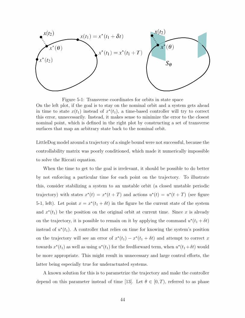
Figure 5-1: Transverse coordinates for orbits in state spaceOn the left plot, if the goal is to stay on the nominal orbit and a system gets aheadin time to state x(t1) instead of x?(t1), a time-based controller will try to correctthis error, unnecessarily. Instead, it makes sense to minimize the error to the closestnominal point, which is defined in the right plot by constructing a set of transversesurfaces that map an arbitrary state back to the nominal orbit.

LittleDog model around a trajectory of a single bound were not successful, because the

controllability matrix was poorly conditioned, which made it numerically impossible

to solve the Riccati equation.

When the time to get to the goal is irrelevant, it should be possible to do better

by not enforcing a particular time for each point on the trajectory. To illustrate

this, consider stabilizing a system to an unstable orbit (a closed unstable periodic

trajectory) with states x?(t) = x?(t + T ) and actions u?(t) = u?(t + T ) (see figure

5-1, left). Let point x = x?(t1 + δt) in the figure be the current state of the system

and x?(t1) be the position on the original orbit at current time. Since x is already

on the trajectory, it is possible to remain on it by applying the command u?(t1 + δt)

instead of u?(t1). A controller that relies on time for knowing the system’s position

on the trajectory will see an error of x?(t1) − x?(t1 + δt) and attempt to correct x

towards x?(t1) as well as using u?(t1) for the feedforward term, when u?(t1+δt) would

be more appropriate. This might result in unnecessary and large control efforts, the

latter being especially true for underactuated systems.

A known solution for this is to parametrize the trajectory and make the controller

depend on this parameter instead of time [13]. Let θ ∈ [0, T ), referred to as phase

44

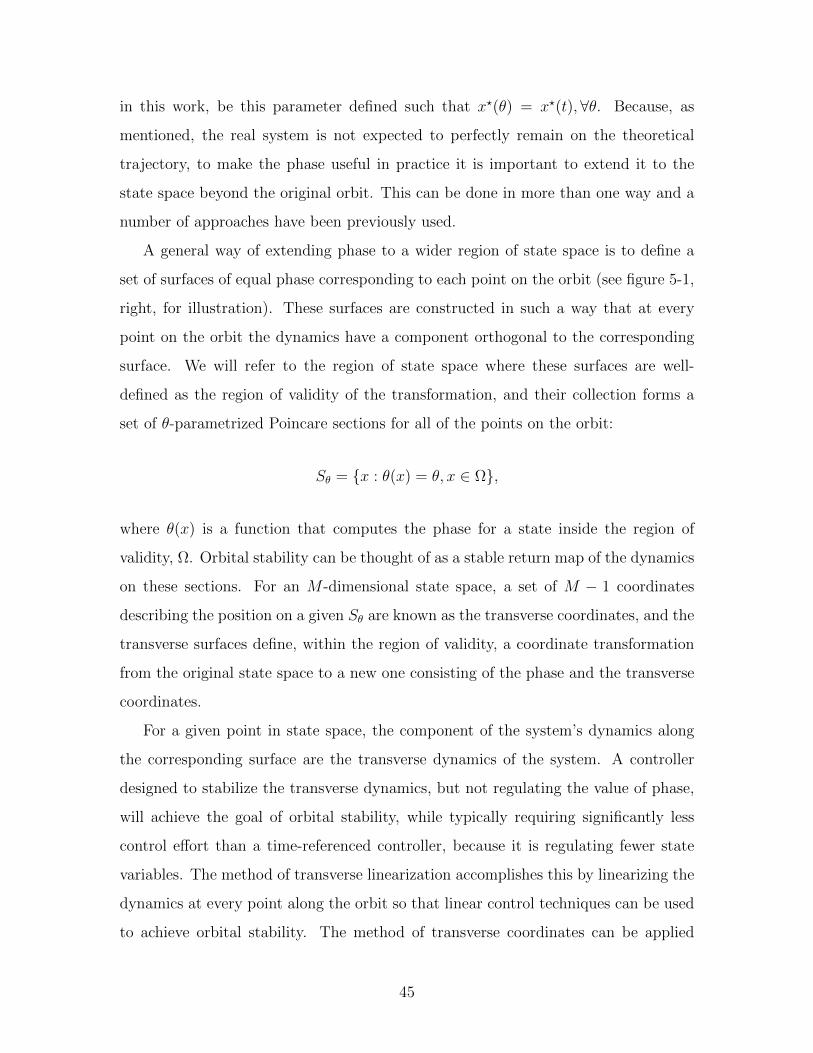
in this work, be this parameter defined such that x?(θ) = x?(t),∀θ. Because, as

mentioned, the real system is not expected to perfectly remain on the theoretical

trajectory, to make the phase useful in practice it is important to extend it to the

state space beyond the original orbit. This can be done in more than one way and a

number of approaches have been previously used.

A general way of extending phase to a wider region of state space is to define a

set of surfaces of equal phase corresponding to each point on the orbit (see figure 5-1,

right, for illustration). These surfaces are constructed in such a way that at every

point on the orbit the dynamics have a component orthogonal to the corresponding

surface. We will refer to the region of state space where these surfaces are well-

defined as the region of validity of the transformation, and their collection forms a

set of θ-parametrized Poincare sections for all of the points on the orbit:

Sθ = x : θ(x) = θ, x ∈ Ω,

where θ(x) is a function that computes the phase for a state inside the region of

validity, Ω. Orbital stability can be thought of as a stable return map of the dynamics

on these sections. For an M -dimensional state space, a set of M − 1 coordinates

describing the position on a given Sθ are known as the transverse coordinates, and the

transverse surfaces define, within the region of validity, a coordinate transformation

from the original state space to a new one consisting of the phase and the transverse

coordinates.

For a given point in state space, the component of the system’s dynamics along

the corresponding surface are the transverse dynamics of the system. A controller

designed to stabilize the transverse dynamics, but not regulating the value of phase,

will achieve the goal of orbital stability, while typically requiring significantly less

control effort than a time-referenced controller, because it is regulating fewer state

variables. The method of transverse linearization accomplishes this by linearizing the

dynamics at every point along the orbit so that linear control techniques can be used

to achieve orbital stability. The method of transverse coordinates can be applied

45

to non-periodic, finite trajectories by substituting the task of stability by that of

minimizing a cost function and adopting the convention that trajectories terminate

when they reach the phase of the goal state. This work uses phase-based finite-horizon

LQR applied to the transverse linearization of the LittleDog dynamics.

As mentioned, the definition of the transverse surfaces and the process of lin-

earization limit the region in which the controller is effective. Appendix A describes

our work on deriving guaranteed regions of stability of a transverse controller on a

simple periodic walking system.

5.1.2 Orthogonal Surfaces

The use of transverse linearization in this work requires a robust and easily com-

putable way of constructing the transverse surfaces for arbitrary planned trajectories.

This can be done by defining the surface at phase θ, Sθ, as a hyperplane orthogonal

to the trajectory at x?(θ) with respect to some distance metric d. Then, the phase

for a state sufficiently close to the trajectory can be computed as

θ(x) = arg minτ‖x?(τ)− x‖d. (5.0)

For a differentiable trajectory this is always well defined locally. The connected region

of state space that includes the trajectory where the minimum is unique is the region

of validity of this definition and depends on the distance metric as well as on the

shape of the trajectory.

This work defines the distance metric in terms of Euclidean distance by choosing

a positive definite matrix W :

‖z‖d = ‖√Wz‖. (5.0)

There is a compelling argument for making W varying with the phase along the

trajectory to increase the region of validity and optimize other properties of the

surfaces, but it is kept constant in this work for simplicity.

46

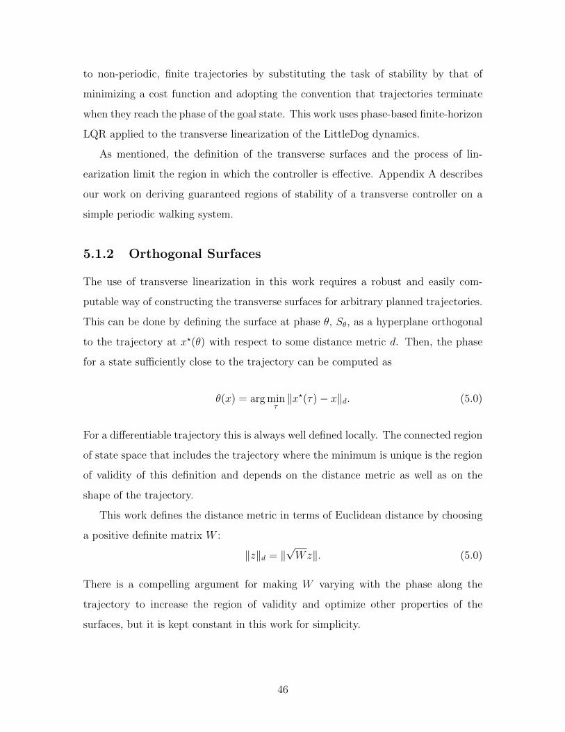
Figure 5-2: State space trajectory of a system with discrete-time inputsFor a system with a continuous state space, but control inputs discretized in time,a control input that works at timestep n − 1 might not be as good half a timesteplater, making the notion of a nominal control input outside of the nodes hard todefine. When trying to apply the method of transverse coordinates, this requirescareful consideration of projection surfaces, phase calculation, and a new concept oforbital stability.

5.1.3 Discrete Approximation

Implementation on a real system usually requires a controller to be converted into

discrete form. If the time interval between adjacent control actions is small in compar-

ison to the timescale of the system’s dynamics, this tends to not be a problem because

there is little difference between the continuous control input and a discretized signal.

However, when the time step is relatively large, the commands might be changing

significantly between two adjacent time steps. For LittleDog, a full bounding motion,

which is the length of time from the moment that a set of legs touches down, lifts off,

and touches down again, might take as little as 50 time steps, only 0.5s. The time

constants of the collision and joint dynamics are significantly faster than the 0.01s

control steps, while the body pitch dynamics can have a time constant of as little as

0.1s. Because of that, even though the underlying system is continuous, the model

developed in section 3 and used in control design is discrete, obtained by integrating a

continuous physics model for 0.01s with a zero-order hold on the control input. In this

case the discretization effects are significant, so, unlike previous implementation of

transverse linearization, the effect of discrete dynamics is explicitly considered when

stabilizing LittleDog bounding.

47

Consider a trajectory of length N for a discrete-time system with dynamics

x[n+ 1] = f(x[n], u[n])

and timestep δt, represented by states x[0], . . . , x[N ] and corresponding control com-

mands u[0], . . . , u[N − 1]. Defining the phase as a discrete variable loses information

about the state, resulting in up to 1 timestep of error in the control command and

could add significant discretization errors. This could be a big issue when the timestep

is relatively large and there is a strong feedforward term, as in the case of LittleDog.

In this case, it is possible to think of the discrete dynamics as an integral over the

continuous dynamics with a continuum of states along the whole trajectory. A contin-

uous trajectory has the benefit of allowing one to define a continuous phase variable

to index into the trajectory, but creates a number of issues as illustrated in Fig-

ure 5-2. First of all, because the control input changes discontinuously between the

timesteps, the derivative of the trajectory is not defined at those times. Therefore,

if the transverse surfaces are constructed according to (5.1.2), they are not defined

at those points and have small regions of validity in the vicinity. Secondly, even if

the transverse coordinates are zero at a point on the trajectory, applying the nominal

control input will not in general make the system remain on the nominal trajectory.

To deal with both of these problems, we interpolate between adjacent timesteps for

the purposes of constructing the transverse surfaces and applying control, as well as

making a number of other approximations.

5.2 Implementation for Control of LittleDog

5.2.1 Phase Variable Selection

Using (5.1.2) to compute the current phase for a point in state space depends on

the choice of W and the method of interpolation for adjacent points on the discrete

trajectory (referred to as nodes when describing them as part of the continuous tra-

jectory). To be as effective as possible, the phase computation should be robust to

48

noise in the state estimates and to errors in the model dynamics and give reasonable

result when the system has large deviations from the nominal trajectory.

Previous studies used one of the kinematic states of the system to determine

the current phase of a robot ([24],[52]). This has the benefit of the phase being

independent from most other variables, separating the states involved in computing

the phase and states that need to be actively controlled, and it is generally easy to

compute. However, this approach is not possible on a robot such as LittleDog, where

within any particular bounding trajectory, none of the angles of the robot increase

or decrease monotonically, and the robot’s configuration might repeat within a given

trajectory. Therefore, a balance between the weights on position and velocity states

is desired for the purpose of phase computation.

We refer to the angle formed between the vertical and the line from the supporting

foot to the center of mass of the robot as the LittleDog pendulum angle or the center

of mass (COM) angle. To first approximation, the dynamics of LittleDog during a

bounding motion is that of a simple pendulum, so we also refer to the COM angle

dynamics as the LittleDog pendulum dynamics. The motions of the legs and the

body can be effectively thought of as an inertial wheel with varying inertia and as

changing the length of the pendulum, and these motions have a large effect on the

dynamics. However, except for near the unstable equilibrium, the COM component of

the dynamics dominate the overall direction during a trajectory. Furthermore, unlike

the position of the joints, which can be easily set to the desired position, the COM

dynamics capture the underactuated nature of the bounding robot, so it is natural to

make the phase computation heavily rely on these states.

Neither the COM angle nor the COM angular velocity are, in general, monotonic

during LittleDog bounding trajectories, but there is a unique pair of these two vari-

ables for each point in all of our bounding trajectories. The COM velocity goes to

zero at certain points in all of the bounding trajectories that we used, so it was im-

possible to rely on the COM angle for phase estimation. However, the estimates of

COM velocity are noisier, which prevents one from heavily relying on them, as well.

As was discussed in Chapter 3 and can be seen in Figure 3-1, the state of LittleDog

49

is described by the body position, the angles of the joints, the pitch, the derivatives of

all these, as well as the positions of the ground contact springs. Using the COM angle

instead of pitch still allows a full description of the state space. Let G be a map from

the state space using the pitch angle and pitch velocity to that using the COM angle

and COM velocity. Both state descriptions are complete, so the map is invertible.

Given a segment (x?[0], . . . , x?[n]) of a discrete trajectory and a current state estimate

x, we compute distances from x to all points on the trajectory, (r0, . . . , rn), as

ri = ‖√W (G(x)− G(x?[i]))‖,

with W heavily weighted towards the COM angle and COM angular velocity and,

although not necessary for this method, diagonal for simplicity. To approximately

find the phase of the closest point on the trajectory, we compute the minimum of a

parabola fit through the 3 lowest values of ri. This is an approximate method to get

θ(x), but in practice we found it to be the most robust to errors in estimation and

model errors.

5.2.2 Effect of Collisions

As described in section 4.3, planned LittleDog trajectories are divided into segments

based on the mode of the dynamics: pendulum mode on back leg, pendulum mode

on front leg, and double support mode. Starting from a planned trajectory and a

terrain map, the division into segments and classification is done by thresholding

on the height of the back and front feet above the terrain. Figure 5-3 shows an

example classification, with red and blue showing the height of the back and front

feet, respectively, and asterisks showing the borders between the segments. The

double support phase is intentionally made larger, to be conservative. Note, that it

is important to accurately detect mode transitions, as transitioning too early or too

late may result in having a state far away from the nominal trajectory or outside the

region of validity, potentially resulting in unexpected collisions or divergence from the

nominal trajectory.

50

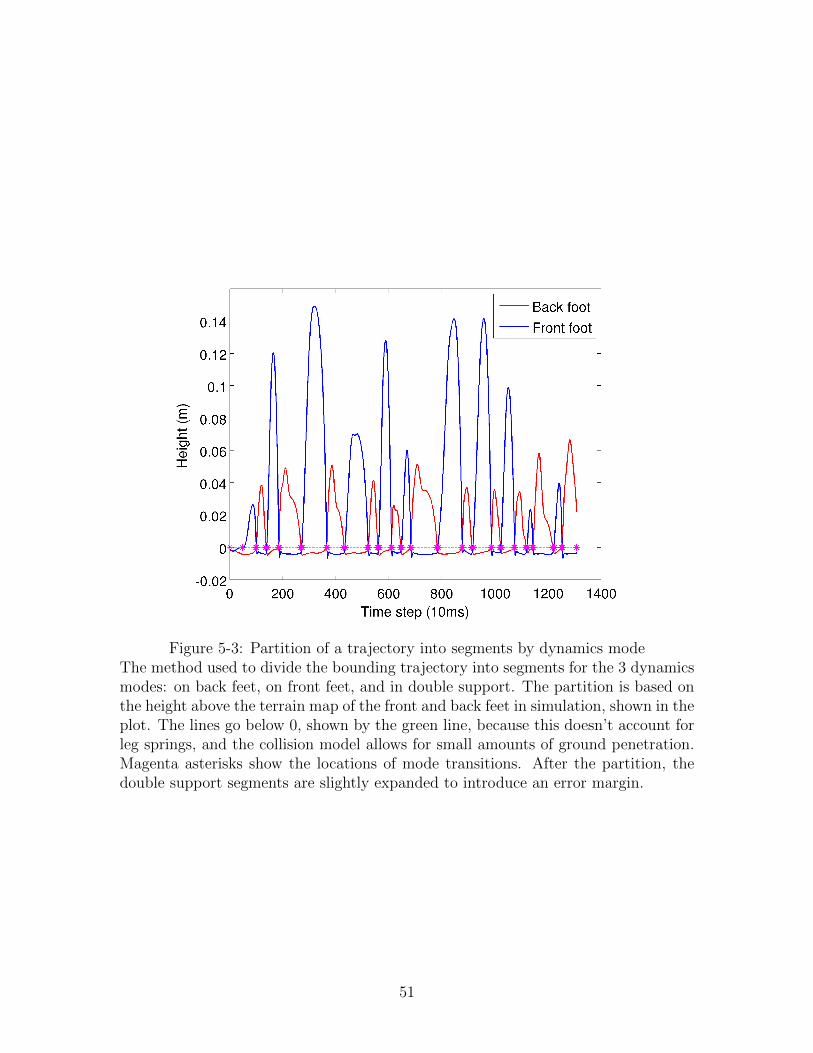
Figure 5-3: Partition of a trajectory into segments by dynamics modeThe method used to divide the bounding trajectory into segments for the 3 dynamicsmodes: on back feet, on front feet, and in double support. The partition is based onthe height above the terrain map of the front and back feet in simulation, shown in theplot. The lines go below 0, shown by the green line, because this doesn’t account forleg springs, and the collision model allows for small amounts of ground penetration.Magenta asterisks show the locations of mode transitions. After the partition, thedouble support segments are slightly expanded to introduce an error margin.

51

Each segment is treated as a separate control problem for the purposes of phase

computation and stabilization of transverse coordinates. The current phase is com-

puted only by considering the pieces of the trajectory in the current segment and,

when the current phase reaches the end of the segment, the system is assumed to tran-

sition into the next mode. There is some overlap between the segments to smooth

out the transition. For transverse coordinate stabilization design, the final state is

the last nominal state in a segment.

The dynamics are stiff near the collisions, so small errors in state estimation or

small model errors might have a large effect on the control input. Because of this and

time delays, it becomes difficult to have beneficial feedback control near the collisions,

so our controller doesn’t stabilize transverse coordinates during the double support

mode (which is, essentially, a continuous collision) and a few time steps prior to the

expected collision, to account for potential model or state estimation errors. Luckily,

ground interactions are stabilizing for pitch in double support mode, so it is not as

necessary to have good feedback during this mode.

5.2.3 LQR in Transverse Coordinates

For each segment of the trajectory that is in pendulum mode of the dynamics, the

commands computed by the RG-RRT planner are augmented by feedback from an

optimal linear controller designed on the linearized transverse dynamics of the sys-

tem. The gains for each time step of the segment are computed offline and are then

interpolated based on the current phase during the execution. Note that there is no

need to smooth the commands coming out of RG-RRT, because of its use of smooth

half-bound motion primitives [46].

Let x[n + 1] = f(x[n], u[n]) represent the pinned (without ground model) dy-

namic model of LittleDog for one of the pendulum modes. Let (x?[0], . . . , x?[N ])

be a segment of the nominal trajectory with all points in the same dynamics mode

and (u?[0], . . . , u?[N − 1]) be the corresponding nominal control input. The surface

52

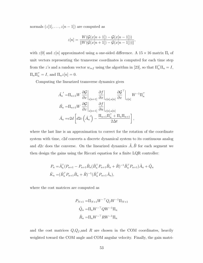
normals (z[1], . . . , z[n− 1]) are computed as

z[n] =W (G(x[n+ 1])− G(x[n− 1]))

‖W (G(x[n+ 1])− G(x[n− 1]))‖,

with z[0] and z[n] approximated using a one-sided difference. A 15× 16 matrix Πi of

unit vectors representing the transverse coordinates is computed for each time step

from the z’s and a random vector wref using the algorithm in [23], so that Π>nΠn = I,

ΠnΠ>n = I, and Πnz[n] = 0.

Computing the linearized transverse dynamics gives

An′=Πn+1W

∂G∂x

∣∣∣∣x[n+1]

∂f

∂x

∣∣∣∣x[n],u[n]

∂G∂x

>∣∣∣∣x[n]

W−1Π>n

Bn =Πn+1W∂G∂x

∣∣∣∣x[n+1]

∂f

∂u

∣∣∣∣x[n],u[n]

An =c2d

[d2c

(An′)− Πn+1Π

>n + ΠnΠn+1

2∆t

],

where the last line is an approximation to correct for the rotation of the coordinate

system with time, c2d converts a discrete dynamical system to its continuous analog

and d2c does the converse. On the linearized dynamics A, B for each segment we

then design the gains using the Riccati equation for a finite LQR controller:

Pn =A>n (Pn+1 − Pn+1Bn(B>n Pn+1Bn + R)−1B>n Pn+1)An + Qn

Kn =(B>n Pn+1Bn + R)−1(B>n Pn+1An),

where the cost matrices are computed as

PN+1 =ΠN+1W−>QfW

−1ΠN+1

Qn =ΠnW−>QW−1Πn

Rn =ΠnW−>RW−1Πn

and the cost matrices Q,Qf ,and R are chosen in the COM coordinates, heavily

weighted toward the COM angle and COM angular velocity. Finally, the gain matri-

53

ces are converted from transverse to COM coordinates:

Kn = KnΠnW.

During runtime, given the current state x, the current phase θ(x) is computed as

described in section 5.2.1. Then, for n such that n ≤ θ < n + 1, Kθ is computed by

cubic spline interpolation from the pair Kn, Kn+1, x?θ and u?θ are both computed by

cubic interpolation from x?[n], x?[n + 1], and u?[n], u?[n + 1], respectively. The

controller produces the motor command given by

u = Kθ(G(x?θ)− G(x)) + u?θ.

Figure 5-4 shows an example of a stabilized segment of a bounding trajectory

on flat with small process noise and small estimation errors. The trajectory starts

at the top and moves towards the bottom of the figure. The asterisks mark the

projection of the states at each time step onto the COM angle and COM angular

velocity plane, forming the trajectories as seen in the figure. At each time step, they

are also projected on the nominal trajectory to compute the current phase.

54

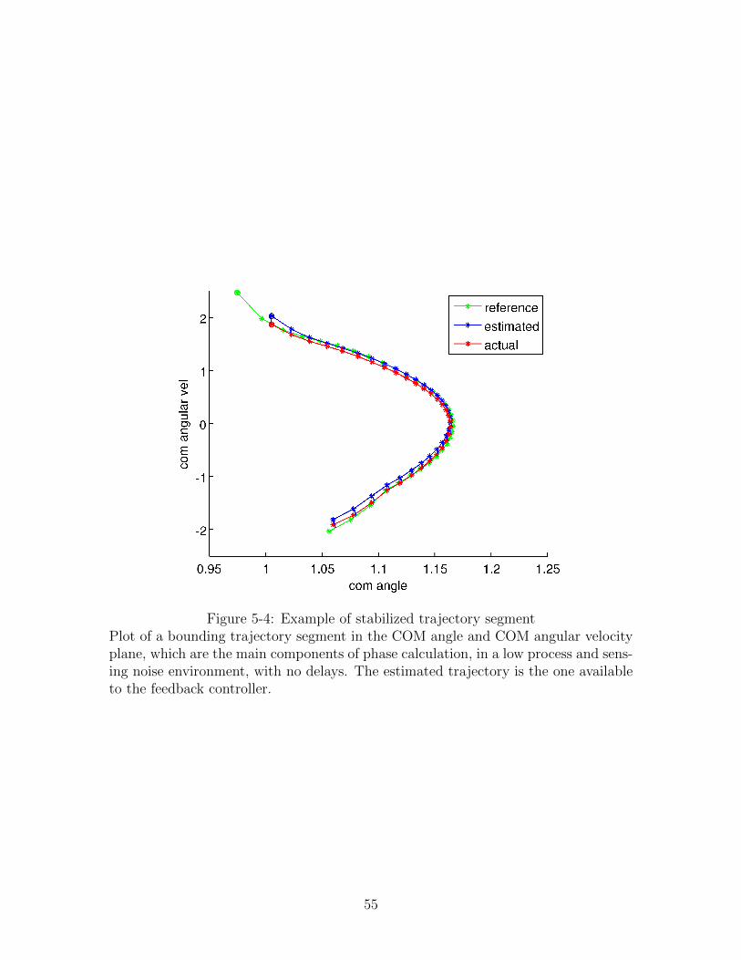
Figure 5-4: Example of stabilized trajectory segmentPlot of a bounding trajectory segment in the COM angle and COM angular velocityplane, which are the main components of phase calculation, in a low process and sens-ing noise environment, with no delays. The estimated trajectory is the one availableto the feedback controller.

55

Chapter 6

Results

6.1 Simulation Results

6.1.1 With Perfect State Knowledge

We have simulated the transverse-linearization controller with a number of RRT-

generated bounding trajectories. For some trajectories over flat terrain in simulation,

we were able to achieve stable bounding even when adding a combination of: 1) slight

Gaussian noise to the state estimate (σ = 0.01 for angles, σ = 0.08 for velocities),

2) significant velocity perturbations up to 1 rad / sec after each ground impact, 3)

model parameter estimation error of up to 1cm in the main body COM position,

and 4) delays of up to 0.04 seconds. In this section we will show some results of

stabilization on two example terrains: bounding up stairs, and bounding over logs.

Since the impact map is the most sensitive and difficult-to-model phase of the

dynamics, we can demonstrate the effectiveness of the controller by adding normally-

distributed random angular velocity perturbation to the passive (stance-ankle) joint

after each impact. Figure 6-1 shows example trajectories of LittleDog bounding up

stairs (perturbations with standard deviation of 0.2 rad/sec), and Figure 6-3 shows

it bounding over logs (perturbations with standard deviation of 0.1 rad/sec).

In each figure, the trajectory of the center of mass is plotted for three cases: 1)

the nominal (unperturbed) motion, as computed by the RRT planner, 2) running the

56

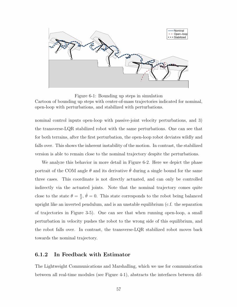
Nominal

Open−loop

Stabilized

Figure 6-1: Bounding up steps in simulationCartoon of bounding up steps with center-of-mass trajectories indicated for nominal,open-loop with perturbations, and stabilized with perturbations.

nominal control inputs open-loop with passive-joint velocity perturbations, and 3)

the transverse-LQR stabilized robot with the same perturbations. One can see that

for both terrains, after the first perturbation, the open-loop robot deviates wildly and

falls over. This shows the inherent instability of the motion. In contrast, the stabilized

version is able to remain close to the nominal trajectory despite the perturbations.

We analyze this behavior in more detail in Figure 6-2. Here we depict the phase

portrait of the COM angle θ and its derivative θ during a single bound for the same

three cases. This coordinate is not directly actuated, and can only be controlled

indirectly via the actuated joints. Note that the nominal trajectory comes quite

close to the state θ = π2, θ = 0. This state corresponds to the robot being balanced

upright like an inverted pendulum, and is an unstable equilibrium (c.f. the separation

of trajectories in Figure 3-5). One can see that when running open-loop, a small

perturbation in velocity pushes the robot to the wrong side of this equilibrium, and

the robot falls over. In contrast, the transverse-LQR stabilized robot moves back

towards the nominal trajectory.

6.1.2 In Feedback with Estimator

The Lightweight Communications and Marshalling, which we use for communication

between all real-time modules (see Figure 4-1), abstracts the interfaces between dif-

57

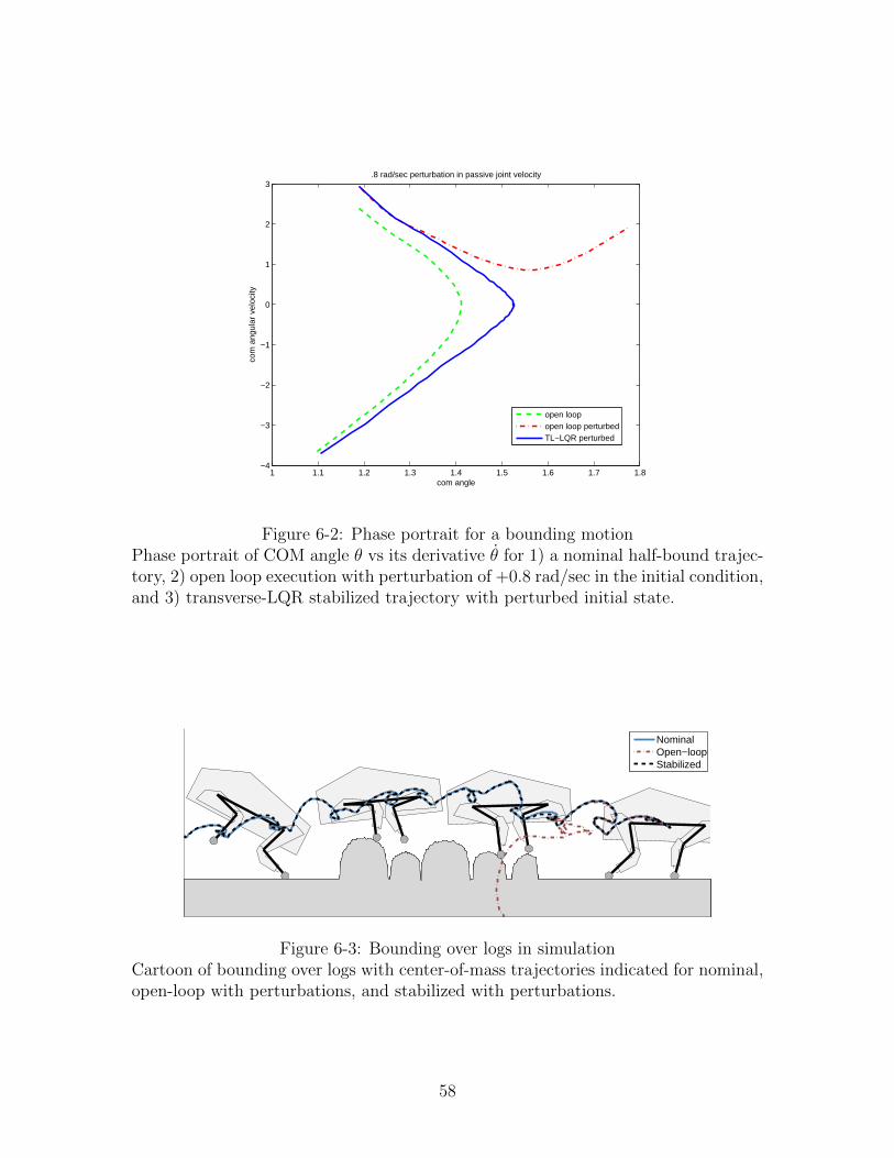
1 1.1 1.2 1.3 1.4 1.5 1.6 1.7 1.8−4

−3

−2

−1

0

1

2

3

com angle

com

ang

ular

vel

ocity

.8 rad/sec perturbation in passive joint velocity

open loopopen loop perturbedTL−LQR perturbed

Figure 6-2: Phase portrait for a bounding motionPhase portrait of COM angle θ vs its derivative θ for 1) a nominal half-bound trajec-tory, 2) open loop execution with perturbation of +0.8 rad/sec in the initial condition,and 3) transverse-LQR stabilized trajectory with perturbed initial state.

NominalOpen−loopStabilized

Figure 6-3: Bounding over logs in simulationCartoon of bounding over logs with center-of-mass trajectories indicated for nominal,open-loop with perturbations, and stabilized with perturbations.

58

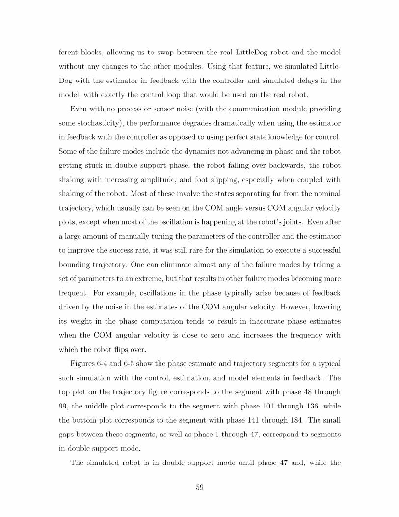
ferent blocks, allowing us to swap between the real LittleDog robot and the model

without any changes to the other modules. Using that feature, we simulated Little-

Dog with the estimator in feedback with the controller and simulated delays in the

model, with exactly the control loop that would be used on the real robot.

Even with no process or sensor noise (with the communication module providing

some stochasticity), the performance degrades dramatically when using the estimator

in feedback with the controller as opposed to using perfect state knowledge for control.

Some of the failure modes include the dynamics not advancing in phase and the robot

getting stuck in double support phase, the robot falling over backwards, the robot

shaking with increasing amplitude, and foot slipping, especially when coupled with

shaking of the robot. Most of these involve the states separating far from the nominal

trajectory, which usually can be seen on the COM angle versus COM angular velocity

plots, except when most of the oscillation is happening at the robot’s joints. Even after

a large amount of manually tuning the parameters of the controller and the estimator

to improve the success rate, it was still rare for the simulation to execute a successful

bounding trajectory. One can eliminate almost any of the failure modes by taking a

set of parameters to an extreme, but that results in other failure modes becoming more

frequent. For example, oscillations in the phase typically arise because of feedback

driven by the noise in the estimates of the COM angular velocity. However, lowering

its weight in the phase computation tends to result in inaccurate phase estimates

when the COM angular velocity is close to zero and increases the frequency with

which the robot flips over.

Figures 6-4 and 6-5 show the phase estimate and trajectory segments for a typical

such simulation with the control, estimation, and model elements in feedback. The

top plot on the trajectory figure corresponds to the segment with phase 48 through

99, the middle plot corresponds to the segment with phase 101 through 136, while

the bottom plot corresponds to the segment with phase 141 through 184. The small

gaps between these segments, as well as phase 1 through 47, correspond to segments

in double support mode.

The simulated robot is in double support mode until phase 47 and, while the

59

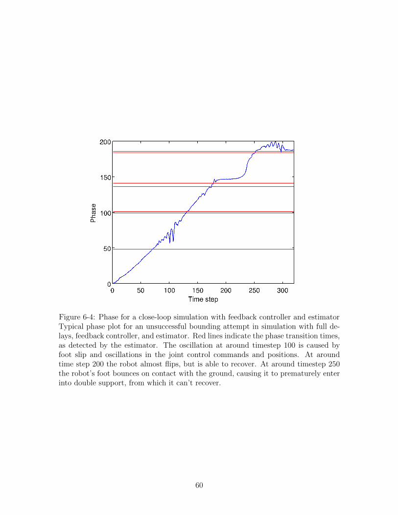
Figure 6-4: Phase for a close-loop simulation with feedback controller and estimatorTypical phase plot for an unsuccessful bounding attempt in simulation with full de-lays, feedback controller, and estimator. Red lines indicate the phase transition times,as detected by the estimator. The oscillation at around timestep 100 is caused byfoot slip and oscillations in the joint control commands and positions. At aroundtime step 200 the robot almost flips, but is able to recover. At around timestep 250the robot’s foot bounces on contact with the ground, causing it to prematurely enterinto double support, from which it can’t recover.

60

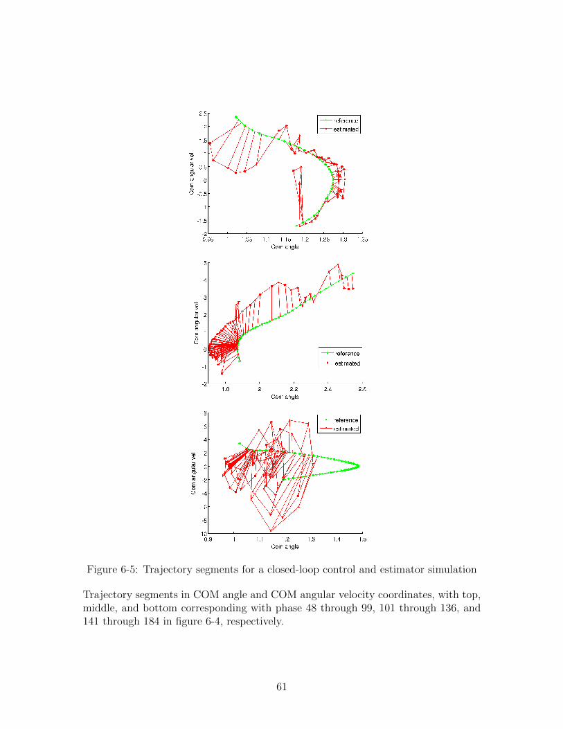
Figure 6-5: Trajectory segments for a closed-loop control and estimator simulation

Trajectory segments in COM angle and COM angular velocity coordinates, with top,middle, and bottom corresponding with phase 48 through 99, 101 through 136, and141 through 184 in figure 6-4, respectively.

61

increase in the phase is monotonic, the slope of the phase averages at 0.69 instead of

1, which indicates that the feedforward term is lagging slightly. In the next segment,

where the robot lifts itself up on the back legs, the foot of the robot slips on the

ground and there is a lot of shaking in the legs, which explains the rapidly jumping

around estimated state trajectory and oscillations in the phase. Oscillations in the

joints produce sharp increases in force at the ground and make the feet more likely to

slip, while foot slip causes the robot to sharply deviate from nominal trajectory and

results in large command changes to the joints. However, it is not clear which one

of these initiates the feedback cycle, which appears and disappears suddenly because

foot slip is a discrete event.

In the next segment the robot is on the front feet between phase 101 through

136, corresponding to the middle plot in Figure 6-5. The trajectory doesn’t stay

close to the nominal, but doesn’t diverge either, and, except for a few outliers and

some jumps towards the end, the controller performs decently on this segment. After

the collision and transition to the back feet, the robot barely recovers from falling

backwards, which is seen as a small slope on the phase plot and as a large clump of

states between COM angles of 0.95 and 1.00. The lowest two angles for points on the

nominal trajectory are 1.00 and 1.05, so it is a significant difference in angle. The

robot manages to make it to the next collision, where the foot slips and bounces,

because the robot is in the wrong state at the moment of ground contact. After the

bounce the robot doesn’t have enough momentum to roll onto the front foot and

continue, so the bounding terminates, as can be seen from the flat-lining phase plot.

6.2 Experimental Results

6.2.1 Open Loop

As discussed in Chapter 3, the model dynamics are not stable around the bounding

trajectories of the robot and even those trajectories generated by identical command

sequences with closely repeated initial conditions diverge quickly. Therefore, one can’t

62

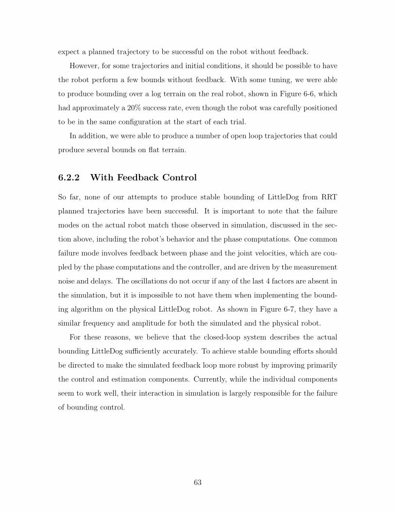
expect a planned trajectory to be successful on the robot without feedback.

However, for some trajectories and initial conditions, it should be possible to have

the robot perform a few bounds without feedback. With some tuning, we were able

to produce bounding over a log terrain on the real robot, shown in Figure 6-6, which

had approximately a 20% success rate, even though the robot was carefully positioned

to be in the same configuration at the start of each trial.

In addition, we were able to produce a number of open loop trajectories that could

produce several bounds on flat terrain.

6.2.2 With Feedback Control

So far, none of our attempts to produce stable bounding of LittleDog from RRT

planned trajectories have been successful. It is important to note that the failure

modes on the actual robot match those observed in simulation, discussed in the sec-

tion above, including the robot’s behavior and the phase computations. One common

failure mode involves feedback between phase and the joint velocities, which are cou-

pled by the phase computations and the controller, and are driven by the measurement

noise and delays. The oscillations do not occur if any of the last 4 factors are absent in

the simulation, but it is impossible to not have them when implementing the bound-

ing algorithm on the physical LittleDog robot. As shown in Figure 6-7, they have a

similar frequency and amplitude for both the simulated and the physical robot.

For these reasons, we believe that the closed-loop system describes the actual

bounding LittleDog sufficiently accurately. To achieve stable bounding efforts should

be directed to make the simulated feedback loop more robust by improving primarily

the control and estimation components. Currently, while the individual components

seem to work well, their interaction in simulation is largely responsible for the failure

of bounding control.

63

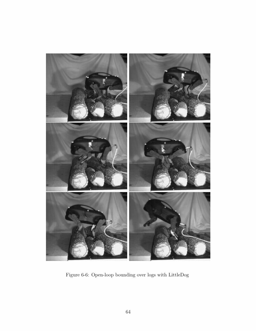
Figure 6-6: Open-loop bounding over logs with LittleDog

64

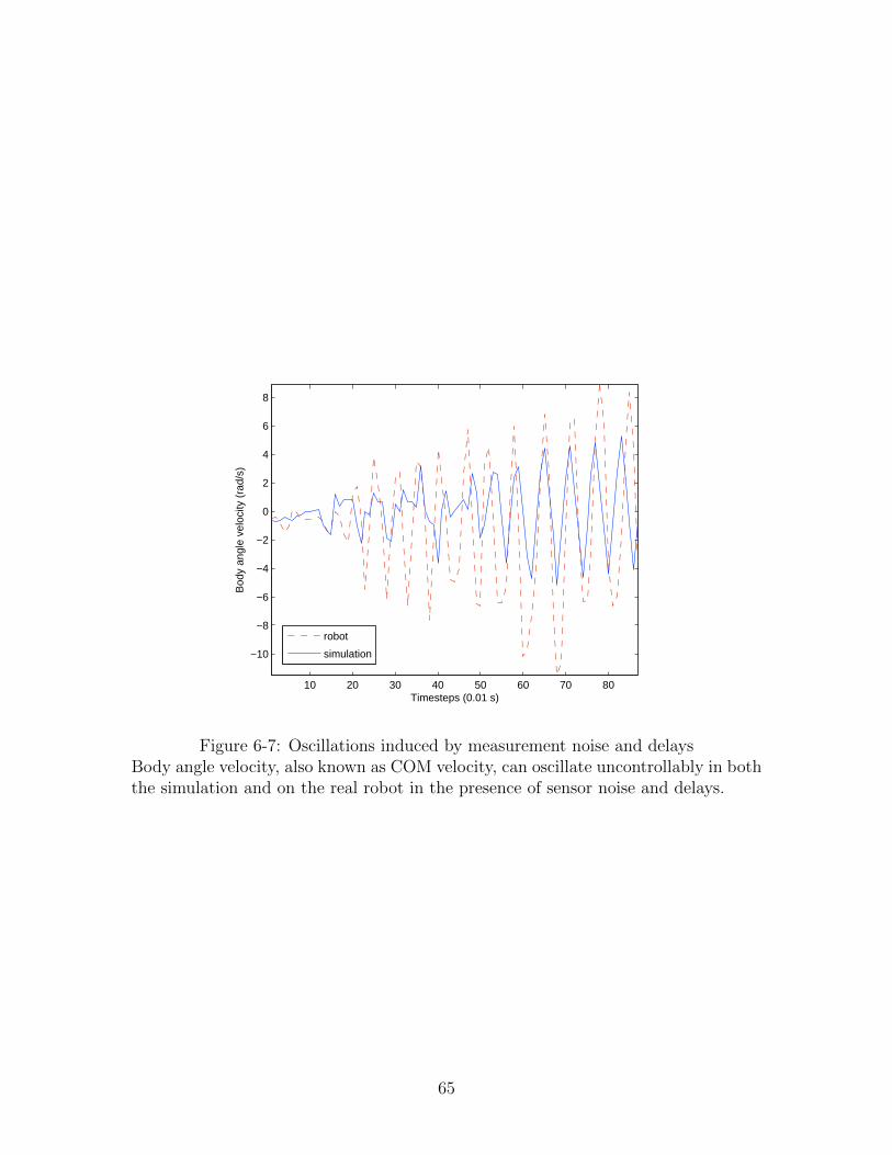
10 20 30 40 50 60 70 80

−10

−8

−6

−4

−2

0

2

4

6

8

Timesteps (0.01 s)

Bod

y an

gle

velo

city

(ra

d/s)

robot

simulation

Figure 6-7: Oscillations induced by measurement noise and delaysBody angle velocity, also known as COM velocity, can oscillate uncontrollably in boththe simulation and on the real robot in the presence of sensor noise and delays.

65

Chapter 7

Summary and Discussion

In this work, we have put together a framework for achieving a stable bounding gait

of the LittleDog robot over rough terrain. We have chosen a model-based control

approach and have developed and identified an accurate planar physics-based model

of LittleDog. The model describes the motions in the joints of the robot and includes

a novel method for ground contact modeling that explicitly incorporates the springs

in the feet of LittleDog. We then altered the Extended Kalman Filter algorithm

to explicitly incorporate the time delays present in the robot’s sensors and used it,

along with the model, to construct a state estimator for the robot. We applied a

transverse linearization controller to trajectories planned using the model, adapting

the controller as necessary to the specifics of having non-negligible time discretization

of motor inputs. We then integrated the controller, estimator, and dynamical model

in simulation, analyzed the system and tuned the components to improve performance

in hopes of transferring it over to the real system.

The model developed, while not perfect, provides an accurate description of the

system’s robot dynamics and even allowed us to generate trajectories that produced

short bounding motions on LittleDog with no feedback. The transverse linearization

controller was highly successful in stabilizing the system in simulation with perfect

state knowledge. The estimator also shows reasonable ability to track the states

of the system and compensate for delays. Unfortunately, when the components get

combined into a feedback loop in simulation, we are not able to produce a stable

66

bounding motion, largely because of the harmful interactions between the estimation

and feedback control algorithms. Implementing these algorithms on the real robot

instead of simulation produces similar behavior in terms of the failure modes of the

system. So, we believe that we can achieve bounding on the actual LittleDog robot

by making the individual components of our control framework more robust and by

minimizing the harmful interaction between them.

The model was developed with the goal of finding a balance between accuracy and

complexity, which mostly relates to state space dimension, in this case. While higher

levels accuracy can be achieved by including the unmodeled effects of backlash in the

joints, joint loading from external forces, and improvements in ground interactions

modeling, particularly in the friction model, all of these improvements would come at

increased complexity for the purposes of planning, estimation, and feedback control.

Currently, the estimator does not use the force sensors in the feet of LittleDog,

which would help in detecting the moment of collision with the ground, an important

time for the control system. Obviously, the accuracy of the estimates, and with it

the whole control loop performance, will improve significantly by using sensors with

lower delays and smaller noise.

There is more room for improvement in the control algorithm. In this work, we

only started to investigate the effects of having large control time steps for transverse

linearization, and more rigorous theoretical understanding is desired to learn how to

best adapt this technique to these types of systems. The weight matrix, W , used

in the definition of the transverse surfaces was constant, and we expect a significant

improvement from applying a good method of varying W along the trajectory or

from constructing the surfaces by directly choosing the orthogonal vector, instead of

using the direction of the dynamics. Finally, note that the finite-time LQR gains

were computed for each segment separately. If the transverse dynamics and collision

gradients are sufficiently reliable, it might be better to compute the solution to the

Riccati equation for LQR across multiple collisions. Above all, what is needed is a

better understanding of the interactions between the estimator and control algorithm

in a complex dynamical system like LittleDog. This would allow a more intelligent

67

selection of the LQR and Kalman Filter gains, which are now designed independently

of each other, to minimize harmful effects and make the overall system more robust.

Although the focus of this work was on the specific task of designing and stabi-

lizing LittleDog bounding trajectories, the approach that was used is very general

and could be applied to controlling many systems, particularly other walking robots,

potentially only by swapping out the dynamics model and changing the estimator to

fit the specifics of the new system. We hope that the work presented here along with

potential improvements listed above would be sufficient in order to solve, or at least

bring closer to solution, truly dynamic locomotion over arbitrary rough terrain on

LittleDog and many other robots.

68

Appendix A

Control Verification

The robustness of a transverse verification controller will be limited by the region of

validity of the transverse coordinates and by the error introduced during linearization

of the dynamics. Estimating the robustness of this approach on the LittleDog robot

currently requires extensive simulation with various initial conditions and perturba-

tions. Because of the high complexity of the problem, it requires an unreasonable

number of computation to generate an accurate estimate. It would be preferable to

have an algorithm that produces robustness guarantees as the controller is generated,

simplifying the analysis and opening the possibility of optimizing over the size of the

controller’s basin of attraction. In pursuit of that goal, we have analyzed the basin

of attraction of the simplest walking system, the Rimless Wheel.

A.1 Rimless Wheel Dynamics

The rimless wheel is a simple planar model of walking and consists of a central

mass with several ‘spokes’ extending radially outward. (See Figure A-1). At any

given moment one of the spokes is pinned at the ground, and the system follows the

dynamics of a simple pendulum, f(θ, θ) = [θ, sin(θ)]′. When another spoke contacts

the ground, the system undergoes an inelastic collision governed by θ+ = cos(2α)θ,

and the new spoke becomes the pinned one.

On a sufficiently inclined slope the system has a stable limit cycle, for which the

69

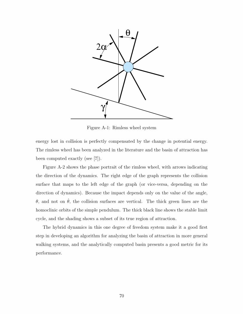
γ

2α

θ

Figure A-1: Rimless wheel system

energy lost in collision is perfectly compensated by the change in potential energy.

The rimless wheel has been analyzed in the literature and the basin of attraction has

been computed exactly (see [7]).

Figure A-2 shows the phase portrait of the rimless wheel, with arrows indicating

the direction of the dynamics. The right edge of the graph represents the collision

surface that maps to the left edge of the graph (or vice-versa, depending on the

direction of dynamics). Because the impact depends only on the value of the angle,

θ, and not on θ, the collision surfaces are vertical. The thick green lines are the

homoclinic orbits of the simple pendulum. The thick black line shows the stable limit

cycle, and the shading shows a subset of its true region of attraction.

The hybrid dynamics in this one degree of freedom system make it a good first

step in developing an algorithm for analyzing the basin of attraction in more general

walking systems, and the analytically computed basin presents a good metric for its

performance.

70

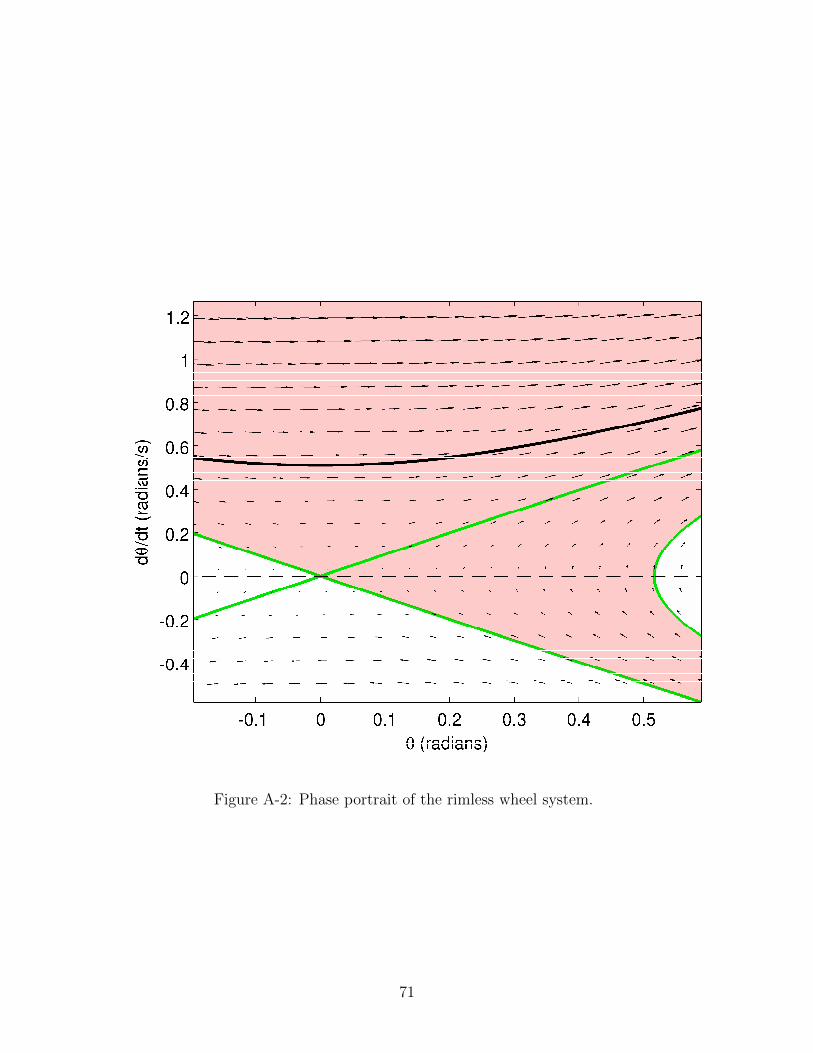
Figure A-2: Phase portrait of the rimless wheel system.

71

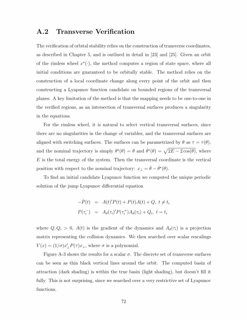
A.2 Transverse Verification

The verification of orbital stability relies on the construction of transverse coordinates,

as described in Chapter 5, and is outlined in detail in [23] and [25]. Given an orbit

of the rimless wheel x?(·), the method computes a region of state space, where all

initial conditions are guaranteed to be orbitally stable. The method relies on the

construction of a local coordinate change along every point of the orbit and then

constructing a Lyapunov function candidate on bounded regions of the transversal

planes. A key limitation of the method is that the mapping needs to be one-to-one in

the verified regions, as an intersection of transversal surfaces produces a singularity

in the equations.

For the rimless wheel, it is natural to select vertical transversal surfaces, since

there are no singularities in the change of variables, and the transversal surfaces are

aligned with switching surfaces. The surfaces can be parametrized by θ as τ = τ(θ),

and the nominal trajectory is simply θ?(θ) = θ and θ?(θ) =√

2E − 2 cos(θ), where

E is the total energy of the system. Then the transversal coordinate is the vertical

position with respect to the nominal trajectory: x⊥ = θ − θ?(θ).

To find an initial candidate Lyapunov function we computed the unique periodic

solution of the jump Lyapunov differential equation

−P (t) = A(t)′P (t) + P (t)A(t) +Q, t 6= ti

P (τ−i ) = Ad(τi)′P (τ+i )Ad(τi) +Qi, t = ti

where Q,Qi > 0, A(t) is the gradient of the dynamics and Ad(τi) is a projection

matrix representing the collision dynamics. We then searched over scalar rescalings

V (x) = (1/σ)x′⊥P (τ)x⊥, where σ is a polynomial.

Figure A-3 shows the results for a scalar σ. The discrete set of transverse surfaces

can be seen as thin black vertical lines around the orbit. The computed basin of

attraction (dark shading) is within the true basin (light shading), but doesn’t fill it

fully. This is not surprising, since we searched over a very restrictive set of Lyapunov

functions.

72

Figure A-3: Regions of Attraction for the rimless wheel limit cycle.Light shaded region is the true RoA. Dark shaded region is the verified RoA.

73

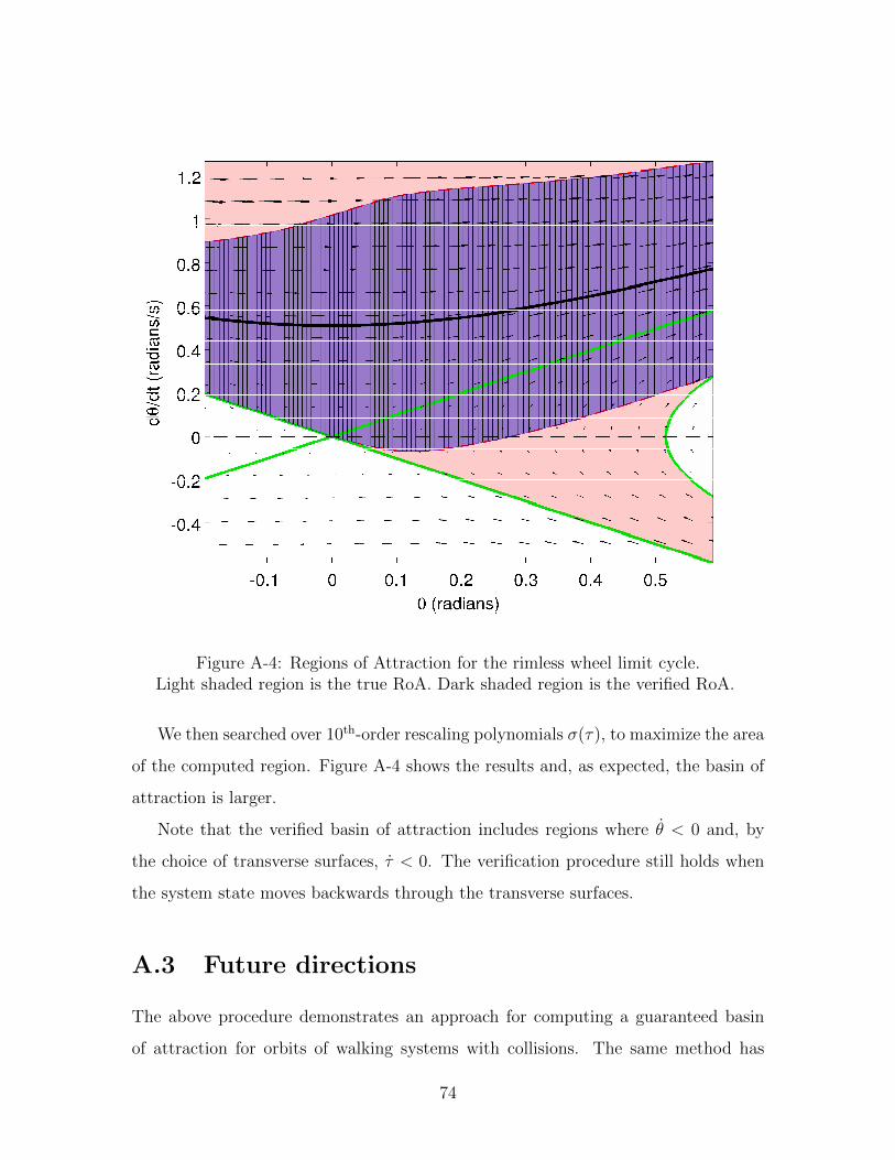
Figure A-4: Regions of Attraction for the rimless wheel limit cycle.Light shaded region is the true RoA. Dark shaded region is the verified RoA.

We then searched over 10th-order rescaling polynomials σ(τ), to maximize the area

of the computed region. Figure A-4 shows the results and, as expected, the basin of

attraction is larger.

Note that the verified basin of attraction includes regions where θ < 0 and, by

the choice of transverse surfaces, τ < 0. The verification procedure still holds when

the system state moves backwards through the transverse surfaces.

A.3 Future directions

The above procedure demonstrates an approach for computing a guaranteed basin

of attraction for orbits of walking systems with collisions. The same method has

74

also been applied to the compass gait system in [25]. Scaling it up to more complex

systems such as LittleDog presents significant challenges, because of high number of

dimensions and the necessity of polynomial approximation to the dynamics, but is an

interesting direction of research for the future.

75

Bibliography

[1] F. Asano, M. Yamakita, N. Kamamichi, and Luo Zhi-Wei. A novel gait gen-eration for biped walking robots based on mechanical energy constraint. IEEETransactions of Robotics and Automation, 20(3):565–573, June 2004.

[2] Andrzej Banaszuk and John Hauser. Feedback linearization of transverse dy-namics for periodic orbits. Systems & Control Letters, 26(2):95 – 105, 1995.

[3] Pedro Berges and Alan Bowling. Rebound, slip, and compliance in the modelingand analysis of discrete impacts in legged locomotion. Journal of Vibration andControl, 12(12):1407 – 1430, 2006.

[4] Katie Byl, Alexander Shkolnik, Sam Prentice, Nicholas Roy, and Russ Tedrake.Reliable dynamic motions for a stiff quadruped. In Proceedings of the 11th In-ternational Symposium on Experimental Robotics (ISER), Athens, Greece, July2008.

[5] Catlin and D.E. Estimation, control, and the discrete Kalman filter. Appliedmathematical sciences. Springer-Verlag, 1989.

[6] C. Chevallereau, G. Abba, Y. Aoustin, F. Plestan, E. R. Westervelt, C. Canudas-De-Wit, and J. W. Grizzle. Rabbit: a testbed for advanced control theory. IEEEControl Systems Magazine, 23(5):57–79, Oct. 2003.

[7] Michael J. Coleman. A Stability Study of a Three-Dimensional Passive-DynamicModel of Human Gait. PhD thesis, Cornell University, 1998.

[8] Steven H. Collins, Andy Ruina, Russ Tedrake, and Martijn Wisse. Efficientbipedal robots based on passive-dynamic walkers. Science, 307:1082–1085, Febru-ary 18 2005.

[9] G. Gilardi and I. Sharf. Literature survey of contact dynamics modelling. Mech-anism and Machine Theory, 37(10):1213 – 1239, 2002.

[10] Goswami, Ambarish, Espiau, Bernard, Keramane, and Ahmed. Limit cycles ina passive compass gait biped and passivity-mimicking control laws. AutonomousRobots, 4:273–286, 1997. 10.1023/A:1008844026298.

76

[11] Ambarish Goswami, Benoit Thuilot, and Bernard Espiau. A study of the passivegait of a compass-like biped robot: symmetry and chaos. International Journalof Robotics Research, 17(12), 1998.

[12] J.W. Grizzle, G. Abba, and F. Plestan. Asymptotically stable walking for bipedrobots: analysis via systems with impulse effects. IEEE Transactions on Auto-matic Control, 46(1):51–64, Jan. 2001.

[13] Jack K. Hale. Ordinary Differential Equations. Robert E. Krieger PublishingCompany, New York, 1980.

[14] Masato Hirose and Kenichi Ogawa. Honda humanoid robots development. Philo-sophical Transactions of the Royal Society, 365(1850):11–19, Jan 2007.

[15] Albert S. Huang, Edwin Olson, and David C. Moore. Lcm: Lightweight commu-nications and marshalling. International Conference on Intelligent Robots andSystems (IROS), 2010 IEEE/RSJ, pages 4057–4062, October 2010.

[16] K. H. Hunt and F. R. E. Crossley. Coefficient of restitution interpreted as damp-ing in vibroimpact. Journal of Applied Mechanics, 42 Series E(2):440–445, 1975.

[17] Fumiya Iida and Russ Tedrake. Minimalistic control of a compass gait robotin rough terrain. In Proceedings of the IEEE/RAS International Conference onRobotics and Automation (ICRA 09), Kobe, Japan, May 2009. IEEE/RAS.

[18] Kajita, S. Kanehiro, F. Kaneko, K. Fujiwara, K. Harada, K. Yokoi, K. Hirukawa,and H. Resolved momentum control: humanoid motion planning based on thelinear and angular momentum. Intelligent Robots and Systems (IROS), Proceed-ings, 2003.

[19] S. Kajita, F. Kanehiro, K. Kaneko, K. Fujiware, K. Harada, K. Yokoi, andH. Hirukawa. Biped walking pattern generation by using preview control of zero-moment point. In Proceedings of the IEEE/RAS International Conference onRobotics and Automation (ICRA 03), pages 1620–1626, Taipei, Taiwan, Septem-ber 2003. IEEE.

[20] Mrinal Kalakrishnan, Jonas Buchli, Peter Pastor, Michael Mistry, and StefanSchaal. Learning, planning, and control for quadruped locomotion over challeng-ing terrain. I. J. Robotic Res., 30(2):236–258, 2011.

[21] Kenji Kaneko, Fumio Kanehiro, Shuuji Kajita, Hirohisa Hirukawa, ToshikazuKawasaki, Masaru Hirata, Kazuhiko Akachi, and Takakatsu Isozumi. Humanoidrobot HRP-2. In Proceedings of the IEEE/RAS International Conference onRobotics and Automation (ICRA 04), pages 1083–1090, New Orleans, LA, May2004. IEEE.

[22] J. Zico Kolter and Andrew Y. Ng. The stanford littledog: A learning and rapidreplanning approach to quadruped locomotion. I. J. Robotic Res., 30(2):150–174,2011.

77

[23] Ian R. Manchester. Transverse dynamics and regions of stability for nonlinearhybrid limit cycles. Proceedings of the 18th IFAC World Congress, extendedversion available online: arXiv:1010.2241 [math.OC], Aug-Sep 2011.

[24] Ian R. Manchester, Uwe Mettin, Fumiya Iida, and Russ Tedrake. Stable dynamicwalking over rough terrain: Theory and experiment. In Proceedings of the Inter-national Symposium on Robotics Research (ISRR), Lucerne, Switzerland, Aug.2009.

[25] Ian R. Manchester, Mark M. Tobenkin, Michael Levashov, and Russ Tedrake.Regions of attraction for hybrid limit cycles of walking robots. Proceedings of the18th IFAC World Congress, extended version available online: arXiv:1010.2247[math.OC], 2011.

[26] D.W. Marhefka and D.E. Orin. Simulation of contact using a nonlinear dampingmodel. In Proceedings of the IEEE/RAS International Conference on Roboticsand Automation (ICRA 96), volume 2, pages 1662–1668 vol.2, Minneapolis, MN,USA, Apr 1996.

[27] Matveev, A. S. Savkin, and A. V. The problem of state estimation via asyn-chronous communication channels with irregular transmission times. IEEETransactions on Automatic Control, 48(4):670–675, 2003.

[28] David Q. Mayne, James B. Rawlings, Christopher V. Rao, and P. O. M. Scokaert.Constrained model predictive control: Stability and optimality. Automatica,36(6):789–814, 2000.

[29] Tad McGeer. Passive dynamic walking. International Journal of Robotics Re-search, 9(2):62–82, April 1990.

[30] Murphy, Michael P., Saunders, Aaron, Moreira, Cassie, Rizzi, Alfred A., Raibert,and Marc. The littledog robot. Int. J. Rob. Res., 30:145–149, February 2011.

[31] Peter D. Neuhaus, Jerry E. Pratt, and Matthew J. Johnson. Comprehensivesummary of the institute for human and machine cognition’s experience withlittledog. I. J. Robotic Res., 30(2):216–235, 2011.

[32] Petersen, I.R., Ugrinovskii, V.A., Savkin, and A.V. Robust control design usingH-8 methods. Communications and control engineering series. Springer, 2000.

[33] James Pippine, Douglas Hackett, and Adam Watson. An overview of the defenseadvanced research projects agency’s learning locomotion program. I. J. RoboticRes., 30(2):141–144, 2011.

[34] Dimitris Pongas, Michael Mistry, and Stefan Schaal. A robust quadruped walkinggait for traversing rough terrain. Proceedings of the IEEE/RAS InternationalConference on Robotics and Automation (ICRA 07), April 2007.

78

[35] Marc Raibert, Kevin Blankespoor, Gabriel Nelson, Rob Playter, and the Big-Dog Team. Bigdog, the rough-terrain quadruped robot. Proceedings of the 17thWorld Congress, The International Federation of Automatic Control, Jul. 2008.

[36] Marc H. Raibert. Legged Robots That Balance. The MIT Press, 1986.

[37] M.H. Raibert, M. Chepponis, and H.B. Brown. Running on four legs as thoughthey were one. IEEE Journal of Robotics and Automation, 2(2):70–82, 1986.

[38] C. David Remy. Optimal Exploitation of Natural Dynamics in Legged Locomo-tion. PhD thesis, ETH ZURICH, 2011.

[39] Y. Sakagami, R. Watanabe, C. Aoyama, S. Matsunaga, and N. Higakiand K. Fu-jimura. The intelligent ASIMO: system overview and integration. In Proceedingsof the IEEE/RSJ International Conference on Intelligent RObots and Systems(IROS 02), volume 3, pages 2478 – 2483, Switzerland, September 2002. IEEE.

[40] Y. Sawaragi, T. Katayama, and Satoru Fujishige. Sequential state estimationwith interrupted observation. Information and Control, 21(1):56–71, August1972.

[41] A. L. Schwab and M. Wisse. Basin of attraction of the simplest walking model.Proceedings of the ASME Design Engineering Technical Conference, 6:531–539,Sep 2001.

[42] Shiriaev, A., Perram, J.W., Canudas de Wit, and C. Constructive tool for orbitalstabilization of underactuated nonlinear systems: Virtual constraints approach.Automatic Control, IEEE Transactions on, 50(8):1164–1176, Aug. 2005.

[43] Anotn S. Shiriaev, Leonid B. Freidovich, and Ian R. Manchester. Can we make arobot ballerina perform a pirouette? orbital stabilization of periodic motions ofunderactuated mechanical systems. Annual Reviews in Control, 32(2):200–211,Dec 2008.

[44] Shkolnik, A., Byl, K., Rohanimanesh, K., Roy, N., Tedrake, and R. Walkingon rough terrain with a position controlled quadruped robot. In InternationalWorkshop on Legged Locomotion for Young Researchers, Cambridge, MA, 2007.

[45] Alexander Shkolnik. Sample-Based Motion Planning in High-Dimensional andDifferentially-Constrained Systems. PhD thesis, MIT, February 2010.

[46] Alexander Shkolnik, Michael Levashov, Ian R. Manchester, and Russ Tedrake.Bounding on rough terrain with the littledog robot. The International Journalof Robotics Research (IJRR), 30(2):192–215, Feb 2011.

[47] M W Spong and F Bullo. Controlled symmetries and passive walking. IEEETransactions on Automatic Control, 50(7):1025–1030, Jul 2005.

79

[48] Russ Tedrake, Ian R. Manchester, Mark M. Tobenkin, and John W. Roberts.LQR-Trees: Feedback motion planning via sums of squares verification. Inter-national Journal of Robotics Research, 29:1038–1052, July 2010.

[49] Nan-Chyuan Tsai, Ray, and A. Compensatability and optimal compensationunder randomly varying distributed delays. In Decision and Control, 1998. Pro-ceedings of the 37th IEEE Conference on, volume 1, pages 772 –777 vol.1, 1998.

[50] Miomir Vukobratovic and Branislav Borovac. Zero-moment point - thirty fiveyears of its life. International Journal of Humanoid Robotics, 1(1):157–173, 2004.

[51] E. R. Westervelt, J. W. Grizzle, and D. E. Koditschek. Hybrid zero dynamicsof planar biped walkers. IEEE Transactions on Automatic Control, 48(1):42–56,Jan 2003.

[52] Eric R. Westervelt, Jessy W. Grizzle, Christine Chevallereau, Jun Ho Choi, andBenjamin Morris. Feedback Control of Dynamic Bipedal Robot Locomotion. CRCPress, Boca Raton, FL, 2007.

[53] Matthew Zucker, Nathan D. Ratliff, Martin Stolle, Joel E. Chestnutt, J. AndrewBagnell, Christopher G. Atkeson, and James Kuffner. Optimization and learningfor rough terrain legged locomotion. I. J. Robotic Res., 30(2):175–191, 2011.

80