Modeling Supply and Demand Dynamics in Energy Systems...

Modeling Supply and Demand

Dynamics in Energy Systems

Planning

André PinaCarlos A. Santos Silva

P. Ferrão

Planning Future Energy Systems

• To design sustainable energy, several

options must be considered:

• Renewable resources

• Energy storage

• Consumer behavior

• Energy efficiency

• Alternative transportation fuels

(biofuels, electricity, others)

• To design effectively, the interactions

between the possible options must be

accounted for:

• Intermittency of renewable resources

• Evolution of energy consumption

• Impact of energy efficiency policies

• Charging of electric vehicles

Energy demand

Energy storage

Renewable energies

Available Tools

Analysis of energy planning tools

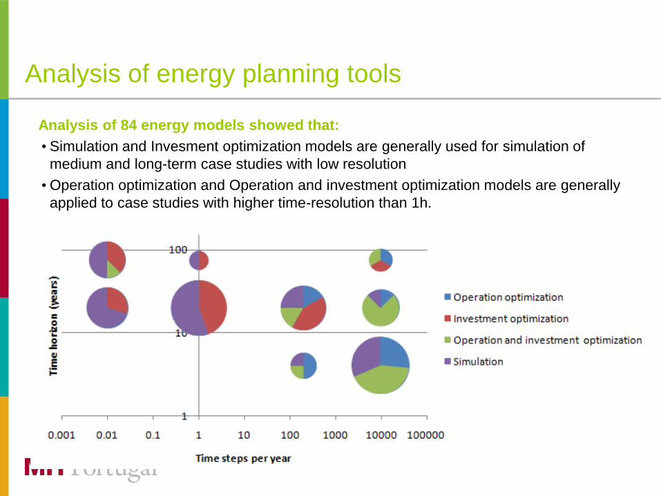
•Analysis of 84 energy models showed that:

• Simulation and Invesment optimization models are generally used for simulation of

medium and long-term case studies with low resolution

• Operation optimization and Operation and investment optimization models are generally

applied to case studies with higher time-resolution than 1h.

Modeling gaps

Tools have very different scopes, resolution and algorithms.

Hour Year

Region /Country

House /Neighborhood

Second

Spatial

resolution

Temporal

resolution

Projections

Optimization

Methodology

Lack the ability to look

into several years

Lack the ability to account

for hourly dynamics

Research goal

Hour Year

Region /Country

House /Neighborhood

Second

Spatial

resolution

Temporal

resolution

Projections

Optimization

Methodology

TIMES-MARKAL

TIMES-MARKAL is an energy-economy-environmental model developed under the

International Energy Agency’s “Energy Technology Systems Analysis Programme”.

•It is a bottom-up optimization model with the following characteristics:

• It does multi-year optimization (computes the least cost path of an energy system for

the specified time frame), but does not have to run every year

• Can be used at the global, multi-regional, national, state/province or community level

• The number and lenght of time slices are defined by the user, within three levels

(seasonal (or monthly), weekdays/weekends, hour of the day), with the user being

able to choose what degree of resolution to give to each process

• Can test a series of policy options, such as CO2 constraints, taxes or subsidies

TIMES model Inputs/outputs

Demand Supply Policy Techno-

economic

Inputs

Outputs

• Drivers

• Demand

curves

• Sectorial

demand

• Energy

services

consumption

• Existing

energy

sources

• Potentials

• Imports

• Costs

• Availability of

resources

• Storage

• Taxes

• Subsidies

• Limitation on

installed

capacities

• Commodity

transformation

technologies:

electricity

generation,

services

consumption

• Costs

• Efficiencies

Installed capacities for each supply and demand technologies, energy fluxes,

final energy prices, total system cost, GHG emissions

Modeling dynamics in TIMES

•The models being developed are new applications of TIMES, as they try to include some

supply and demand dynamics, with higher than usual time resolution.

•Each model is divided into 288 time periods of the year:

• 4 seasons

• 3 days per season (Saturday, Sunday and weekday)

• 24h per day Main new feature

•Supply dynamics were included in the wind, hydro and geothermal resources, as different

periods have different availabilities

•11 different sectors for electricity demand, with the domestic sector divided in 9 subsectors.

Each sector and subsector has a different load curve for each day.

•Three models have been built using TIMES: São Miguel, Flores and Portugal (CCS, Waves)

Modeling São Miguel island with TIMES

The reconstructed load curves show that the model

is able to estimate with some accuracy the evolution

of the demand curve through the years.

Some problems still exist in the model as weekdays

are usually overestimated and Sundays are

underestimated.Reconstructed load curve

Average relative error for each hour of each type of day

Average relative error for each day

Modeling São Miguel island with TIMES

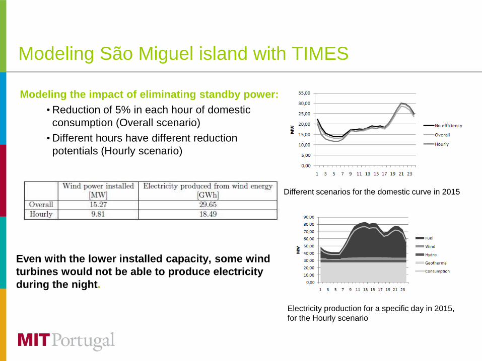
•Modeling the impact of eliminating standby power:

• Reduction of 5% in each hour of domestic

consumption (Overall scenario)

• Different hours have different reduction

potentials (Hourly scenario)

Even with the lower installed capacity, some wind

turbines would not be able to produce electricity

during the night.

Electricity production for a specific day in 2015,

for the Hourly scenario

Different scenarios for the domestic curve in 2015

Modeling Flores island with TIMES

•Scenario based approach to study different future energy options:

• General efficiency

• If there is an increase in overall energy efficiency, demand growth is

reduced to 50% of what it would have been using a linear trend

• No standby power

• Gradually eliminate stand-by power (starting in 2011 and disappearing

completely by 2015). Stand-by power is estimated to account for 5% of the

electricity consumed in the domestic sector in Portugal

• Dynamic demand

• Gradually enable washers, dryers and dish washing machines to be

operated remotely by the grid operator when it is more convenient. Start of

introduction in 2013, with all machines having this capability by 2018.

Modeling Flores island with TIMES

•Higher demand growths lead to larger investments in renewable energies, thus

allowing a higher penetration of renewable energies.

•The load shifting capabilities were used to increase the capacity factors of the

installed renewables, and postpone the need to install more generation

capacity.

Penetration of renewables Fraction of load shifted

Comparison with other modeling methodologies

– Flores case study (Gustavo+Vitor)

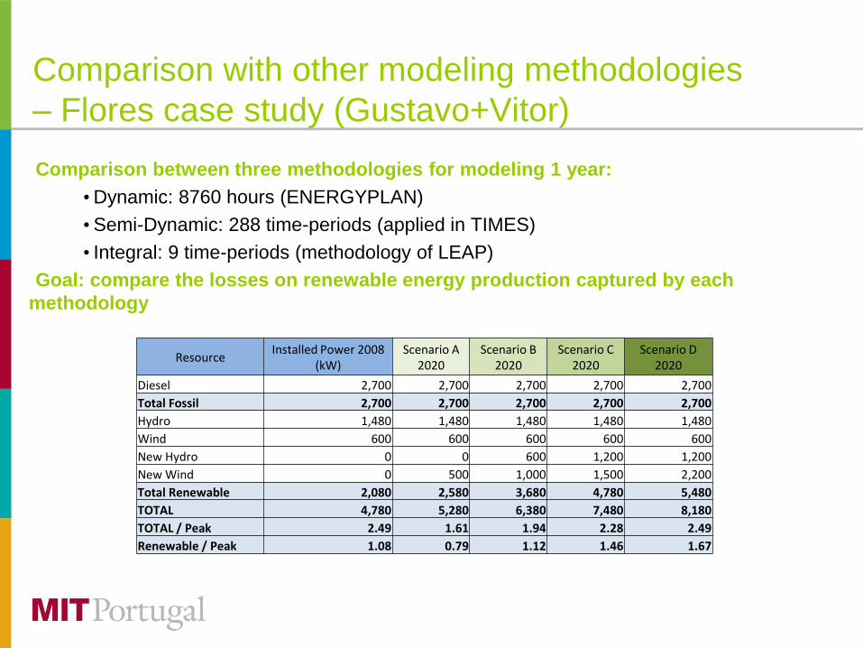
•Comparison between three methodologies for modeling 1 year:

• Dynamic: 8760 hours (ENERGYPLAN)

• Semi-Dynamic: 288 time-periods (applied in TIMES)

• Integral: 9 time-periods (methodology of LEAP)

•Goal: compare the losses on renewable energy production captured by each

methodology

ResourceInstalled Power 2008

(kW)Scenario A

2020Scenario B

2020Scenario C

2020Scenario D

2020

Diesel 2,700 2,700 2,700 2,700 2,700

Total Fossil 2,700 2,700 2,700 2,700 2,700

Hydro 1,480 1,480 1,480 1,480 1,480

Wind 600 600 600 600 600

New Hydro 0 0 600 1,200 1,200

New Wind 0 500 1,000 1,500 2,200

Total Renewable 2,080 2,580 3,680 4,780 5,480

TOTAL 4,780 5,280 6,380 7,480 8,180

TOTAL / Peak 2.49 1.61 1.94 2.28 2.49

Renewable / Peak 1.08 0.79 1.12 1.46 1.67

Comparison with other modeling methodologies

– Flores case study

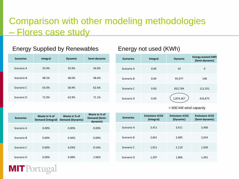
Scenarios Integral Dynamic Semi-dynamic

Scenario A 33.9% 33.9% 34.0%

Scenario B 48.5% 48.0% 48.6%

Scenario C 63.0% 58.9% 62.6%

Scenario D 72.9% 63.9% 71.1%

Scenarios Integral DynamicEnergy wasted kWh

(Semi-dynamic)

Scenario A 0.00 10 0

Scenario B 0.00 95,977 148

Scenario C 0.00 832,764 111,351

Scenario D 0.00 1,874,367 424,675

ScenariosWaste in % of

Demand (Integral)Waste in % of

Demand (Dynamic)

Waste in % of Demand (Semi-

dynamic)

Scenario A 0.00% 0.00% 0.00%

Scenario B 0.00% 0.46% 0.00%

Scenario C 0.00% 4.03% 0.54%

Scenario D 0.00% 9.08% 2.06%

ScenariosEmissions tCO2

(Integral)Emissions tCO2

(Dynamic)Emissions tCO2 (Semi-dynamic)

Scenario A 3,411 3,411 3,406

Scenario B 2,661 2,685 2,654

Scenario C 1,911 2,119 1,930

Scenario D 1,397 1,866 1,491

Energy Supplied by Renewables Energy not used (KWh)

> 600 kW wind capacity

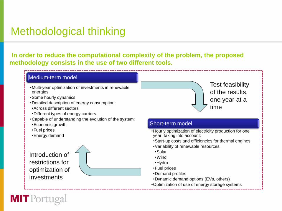
Methodological thinking

•In order to reduce the computational complexity of the problem, the proposed

methodology consists in the use of two different tools.

Medium-term model

•Multi-year optimization of investments in renewable energies

•Some hourly dynamics

•Detailed description of energy consumption:

•Across different sectors

•Different types of energy carriers

•Capable of understanding the evolution of the system:

•Economic growth

•Fuel prices

•Energy demand

Short-term model

•Hourly optimization of electricity production for one year, taking into account:

•Start-up costs and efficiencies for thermal engines

•Variability of renewable resources

•Solar

•Wind

•Hydro

•Fuel prices

•Demand profiles

•Dynamic demand options (EVs, others)

•Optimization of use of energy storage systems

Test feasibility

of the results,

one year at a

time

Introduction of

restrictions for

optimization of

investments

Methodological thinking

TIMES (4 seasons, 3 days, 24h) + Short-time model for key years

- Installed capacities

- Energy consumption changes

- New technologies

- Capacity factors for each plant

- Minimum installed capacity constraints

- Assessment of load dynamics reliabilityMATLAB or

ENERGYPLAN

TIMES

- Scenarios for capacities that can be installed (including storage technologies)

- More robust results regarding power system operation reliability and security

Short-term model for S. Miguel

•MATLAB model being developed by Gonçalo Pereira (MSc)

Inputs

• Installed capacities for electricity generation by source

• Energy storage size and capacity

• Overall electricity demand growth

Data generation

• Electricity demand curve for the whole year

• Hourly availability for each renewable resource

• For wind energy, historical hourly capacity factors for other islands are used

Optimization outputs

• Electricity production by source

• Charge and discharge of energy storage unit

0

0,1

0,2

0,3

0,4

0,5

0,6

0,7

1 713

19

25

31

37

43

49

55

61

67

73

79

85

91

97

10

31

09

11

5

71EOPF 2009

74EOGR 2006

Application of current methodology to SM

The proposed methodology was tested using the São

Miguel TIMES model.

•The model had to make two decisions:

• When should the 2 x 10 MW Geothermal facilities be

installed

• What amount of wind energy should it install and

when

•The methodology was applied separately for the two

decisions.

•Operation conditions:

• Geothermal: the plant must have a capacity factor of

90% or higher for at least 95% of the time.

• Wind: the wind turbines produce at least 90% of the

nominal capacity factor.


•Total installed capacity of wind energy after each TIMES iteration.

•Some notes:

• TIMES processing is the first iteration of TIMES, without any constraint.

• Iteration 1 is the last iteration of the Geothermal decision process, and the first

of the Wind decision process.

• Iteration 10 was the last iteration of the Wind decision process.


•Results for the iteration TIMES processing


•Results for iteration 1


•Results for iteration 10

Application of current methodology to Portugal

• In 2010, renewables produced

~50% of all the electricity in

Portugal

•Some periods during the Winter

time had excesses of renewable

electricity

•The investment in renewable

generation capacity should be

analysed with high temporal

resolution


•Application of methodology with TIMES

and EnergyPLAN.

• Time horizon of 2005-2050.

•Mainland Portugal case study

• Operation conditions:

• Maximization of renewable energy

penetration such that the last installed MW

produces at least 90% of its potential

capacity factor

• 2 scenarios concerning installed capacity

for hydro pump storage (Current capacity

of 1036 vs expected capacity of 4302)

• Assumed gradual reduction of CO2

emissions to ~30% of 2005 levels in 2050

START

InitializationYear = start, i = 1

Investment optimization model

Operation optimization model

Operation conditions

i = i + 1

Year = end

END

Year = Year + 1


1st iteration

Last iteration

Next Methodological Step

TIMES (4 seasons, 3 days, 24h) + Short-time model for key years

- Installed capacities

- Energy consumption changes

- New technologies

- Capacity factors for each plant

- Minimum installed capacity constraints

- Assessment of load dynamics reliabilityMATLAB or

ENERGYPLAN

TIMES

DPLAN(?)

Other ideas going on:

NODES (João Claro, João Sousa)

Wind forecast using soft-computing

Flexible Networked System Design Under Uncertainty:

A Case Study in Long-Term Energy Planning

Wind forecasting using sof-computing

Wind forecasting using soft-computing

Modeling Supply and Demand Dynamics in Energy Systems...

Documents

Transcript of Modeling Supply and Demand Dynamics in Energy Systems...