Modeling Simulation Implementation - cvut.czradio.feld.cvut.cz/matlab/pdf_doc/ncd/ncd_blks.pdf · 2...

SIMULINKDynamic System Simulation for MATLAB

Modeling

Simulation

Implementation

Nonlinear Control Design Blockset User’s GuideVersion 5

How to Contact The MathWorks:

508-647-7000 Phone

508-647-7001 Fax

The MathWorks, Inc. Mail24 Prime Park WayNatick, MA 01760-1500

http://www.mathworks.com Webftp.mathworks.com Anonymous FTP servercomp.soft-sys.matlab Newsgroup

[email protected] Technical [email protected] Product enhancement [email protected] Bug [email protected] Documentation error [email protected] Subscribing user [email protected] Order status, license renewals, [email protected] Sales, pricing, and general information

Nonlinear Control Design Blockset User’s Guide COPYRIGHT 1993 - 1997 by The MathWorks, Inc. All Rights Reserved.The software described in this document is furnished under a license agreement. The software may be used or copied only under the terms of the license agreement. No part of this manual may be photocopied or repro-duced in any form without prior written consent from The MathWorks, Inc.

U.S. GOVERNMENT: If Licensee is acquiring the software on behalf of any unit or agency of the U. S. Government, the following shall apply:

(a) for units of the Department of Defense: RESTRICTED RIGHTS LEGEND: Use, duplication, or disclosure by the Government is subject to restric-tions as set forth in subparagraph (c)(1)(ii) of the Rights in Technical Data and Computer Software Clause at DFARS 252.227-7013.(b) for any other unit or agency: NOTICE - Notwithstanding any other lease or license agreement that may pertain to, or accompany the delivery of, the computer software and accompanying documentation, the rights of the Government regarding its use, reproduction and disclosure are as set forth in Clause 52.227-19(c)(2) of the FAR. Contractor/manufacturer is The MathWorks Inc., 24 Prime Park Way, Natick, MA 01760-1500.

MATLAB, Simulink, Handle Graphics, and Real-Time Workshop are registered trademarks and Stateflow and Target Language Compiler are trademarks of The MathWorks, Inc.

Other product or brand names are trademarks or registered trademarks of their respective holders.

Printing History: September 1993 First printingApril 1997 Second printing (for MATLAB 5)

☎

✉

@

Contents

1Introduction

System Requirements . . . . . . . . . . . . . . . . . . . . . . . . . . . . . . . . . 1-3

Default Window Size . . . . . . . . . . . . . . . . . . . . . . . . . . . . . . . . . . 1-3

Installation Instructions . . . . . . . . . . . . . . . . . . . . . . . . . . . . . . 1-3

Typographical Conventions . . . . . . . . . . . . . . . . . . . . . . . . . . . 1-3

2Tutorial

Quick Start . . . . . . . . . . . . . . . . . . . . . . . . . . . . . . . . . . . . . . . . . . . 2-3

A Control Design Example . . . . . . . . . . . . . . . . . . . . . . . . . . . . . 2-5NCD Startup . . . . . . . . . . . . . . . . . . . . . . . . . . . . . . . . . . . . . . . . 2-5Adjusting Constraints . . . . . . . . . . . . . . . . . . . . . . . . . . . . . . . . . 2-6Running the Optimization . . . . . . . . . . . . . . . . . . . . . . . . . . . . 2-11Adding Uncertainty . . . . . . . . . . . . . . . . . . . . . . . . . . . . . . . . . . 2-13

A System Identification Problem . . . . . . . . . . . . . . . . . . . . . . 2-16NCD Startup . . . . . . . . . . . . . . . . . . . . . . . . . . . . . . . . . . . . . . . 2-16Adjusting Constraints . . . . . . . . . . . . . . . . . . . . . . . . . . . . . . . . 2-19Running the Optimization . . . . . . . . . . . . . . . . . . . . . . . . . . . . 2-21

Solving the Optimization Problem . . . . . . . . . . . . . . . . . . . . . 2-24

NCD Blockset Command Line Interaction . . . . . . . . . . . . . . 2-25

NCD and the SIMULINK Accelerator . . . . . . . . . . . . . . . . . . . 2-26

i

ii Contents

Printing a NCD Blockset Constraint Figure . . . . . . . . . . . . 2-26References . . . . . . . . . . . . . . . . . . . . . . . . . . . . . . . . . . . . . . . 2-26

3Problem Formulation

Actuation Limits vs State Constraints (Physical vs Design Constraints) . . . . . . . . . . . . . . . . . . . . . . . 3-3

Minimizing Integrated Positive Signals (Control Energy) . 3-3

Noise Inputs . . . . . . . . . . . . . . . . . . . . . . . . . . . . . . . . . . . . . . . . . . 3-4

Tracking . . . . . . . . . . . . . . . . . . . . . . . . . . . . . . . . . . . . . . . . . . . . . 3-5

Disturbance Rejection . . . . . . . . . . . . . . . . . . . . . . . . . . . . . . . . . 3-5

System Identification . . . . . . . . . . . . . . . . . . . . . . . . . . . . . . . . . . 3-5

Model Following . . . . . . . . . . . . . . . . . . . . . . . . . . . . . . . . . . . . . . 3-5

Adaptive Control . . . . . . . . . . . . . . . . . . . . . . . . . . . . . . . . . . . . . . 3-6

MIMO Systems . . . . . . . . . . . . . . . . . . . . . . . . . . . . . . . . . . . . . . . . 3-6

Multimode Control . . . . . . . . . . . . . . . . . . . . . . . . . . . . . . . . . . . . 3-6

Gain Scheduling . . . . . . . . . . . . . . . . . . . . . . . . . . . . . . . . . . . . . . 3-7

Repeated Parameter Problems . . . . . . . . . . . . . . . . . . . . . . . . . 3-7

Simultaneous Stabilization . . . . . . . . . . . . . . . . . . . . . . . . . . . . 3-8

Controller Pole (Zero) Placement . . . . . . . . . . . . . . . . . . . . . . . 3-8

Strong Stabilization . . . . . . . . . . . . . . . . . . . . . . . . . . . . . . . . . . . 3-9

4Case Studies

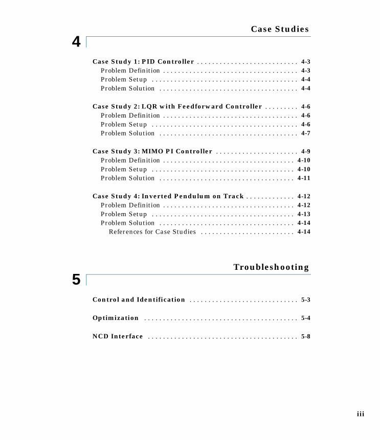
Case Study 1: PID Controller . . . . . . . . . . . . . . . . . . . . . . . . . . . 4-3Problem Definition . . . . . . . . . . . . . . . . . . . . . . . . . . . . . . . . . . . . 4-3Problem Setup . . . . . . . . . . . . . . . . . . . . . . . . . . . . . . . . . . . . . . . 4-4Problem Solution . . . . . . . . . . . . . . . . . . . . . . . . . . . . . . . . . . . . . 4-4

Case Study 2: LQR with Feedforward Controller . . . . . . . . . 4-6Problem Definition . . . . . . . . . . . . . . . . . . . . . . . . . . . . . . . . . . . . 4-6Problem Setup . . . . . . . . . . . . . . . . . . . . . . . . . . . . . . . . . . . . . . . 4-6Problem Solution . . . . . . . . . . . . . . . . . . . . . . . . . . . . . . . . . . . . . 4-7

Case Study 3: MIMO PI Controller . . . . . . . . . . . . . . . . . . . . . . 4-9Problem Definition . . . . . . . . . . . . . . . . . . . . . . . . . . . . . . . . . . . 4-10Problem Setup . . . . . . . . . . . . . . . . . . . . . . . . . . . . . . . . . . . . . . 4-10Problem Solution . . . . . . . . . . . . . . . . . . . . . . . . . . . . . . . . . . . . 4-11

Case Study 4: Inverted Pendulum on Track . . . . . . . . . . . . . 4-12Problem Definition . . . . . . . . . . . . . . . . . . . . . . . . . . . . . . . . . . . 4-12Problem Setup . . . . . . . . . . . . . . . . . . . . . . . . . . . . . . . . . . . . . . 4-13Problem Solution . . . . . . . . . . . . . . . . . . . . . . . . . . . . . . . . . . . . 4-14

References for Case Studies . . . . . . . . . . . . . . . . . . . . . . . . . 4-14

5Troubleshooting

Control and Identification . . . . . . . . . . . . . . . . . . . . . . . . . . . . . 5-3

Optimization . . . . . . . . . . . . . . . . . . . . . . . . . . . . . . . . . . . . . . . . . 5-4

NCD Interface . . . . . . . . . . . . . . . . . . . . . . . . . . . . . . . . . . . . . . . . 5-8

iii

iv Contents

6Reference

Object Manipulation . . . . . . . . . . . . . . . . . . . . . . . . . . . . . . . . . . 6-2Cursor Modes . . . . . . . . . . . . . . . . . . . . . . . . . . . . . . . . . . . . . . . . 6-2Manipulating Constraints . . . . . . . . . . . . . . . . . . . . . . . . . . . . . . 6-2

Using the Mouse . . . . . . . . . . . . . . . . . . . . . . . . . . . . . . . . . . . 6-2Using the Keyboard . . . . . . . . . . . . . . . . . . . . . . . . . . . . . . . . . 6-3Using Edit Menu and Control Panel . . . . . . . . . . . . . . . . . . . 6-4

NCD Blockset Menus . . . . . . . . . . . . . . . . . . . . . . . . . . . . . . . . . . 6-5

File Menu . . . . . . . . . . . . . . . . . . . . . . . . . . . . . . . . . . . . . . . . . . . . 6-6

Edit Menu . . . . . . . . . . . . . . . . . . . . . . . . . . . . . . . . . . . . . . . . . . . . 6-8

Options Menu . . . . . . . . . . . . . . . . . . . . . . . . . . . . . . . . . . . . . . . . . 6-9

Optimization Menu . . . . . . . . . . . . . . . . . . . . . . . . . . . . . . . . . . . 6-12

Style Menu . . . . . . . . . . . . . . . . . . . . . . . . . . . . . . . . . . . . . . . . . . 6-14

NCD Blockset Control Panel . . . . . . . . . . . . . . . . . . . . . . . . . . 6-15

AAppendix

Optimization Details . . . . . . . . . . . . . . . . . . . . . . . . . . . . . . . . . . A-3Problem Formulation Details . . . . . . . . . . . . . . . . . . . . . . . . . . . A-3Optimization Algorithmic Details . . . . . . . . . . . . . . . . . . . . . . . . A-7

Representation of Time Domain Constraints . . . . . . . . . . . A-10

NCD Global Variable ncdStruct . . . . . . . . . . . . . . . . . . . . . . . A-11

LQR Design for Inverted Pendulum . . . . . . . . . . . . . . . . . . . A-14

1

Introduction

1 Introduction

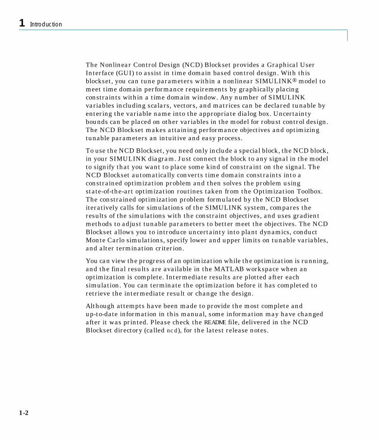
The Nonlinear Control Design (NCD) Blockset provides a Graphical User Interface (GUI) to assist in time domain based control design. With this blockset, you can tune parameters within a nonlinear SIMULINK® model to meet time domain performance requirements by graphically placing constraints within a time domain window. Any number of SIMULINK variables including scalars, vectors, and matrices can be declared tunable by entering the variable name into the appropriate dialog box. Uncertainty bounds can be placed on other variables in the model for robust control design. The NCD Blockset makes attaining performance objectives and optimizing tunable parameters an intuitive and easy process.

To use the NCD Blockset, you need only include a special block, the NCD block, in your SIMULINK diagram. Just connect the block to any signal in the model to signify that you want to place some kind of constraint on the signal. The NCD Blockset automatically converts time domain constraints into a constrained optimization problem and then solves the problem using state-of-the-art optimization routines taken from the Optimization Toolbox. The constrained optimization problem formulated by the NCD Blockset iteratively calls for simulations of the SIMULINK system, compares the results of the simulations with the constraint objectives, and uses gradient methods to adjust tunable parameters to better meet the objectives. The NCD Blockset allows you to introduce uncertainty into plant dynamics, conduct Monte Carlo simulations, specify lower and upper limits on tunable variables, and alter termination criterion.

You can view the progress of an optimization while the optimization is running, and the final results are available in the MATLAB workspace when an optimization is complete. Intermediate results are plotted after each simulation. You can terminate the optimization before it has completed to retrieve the intermediate result or change the design.

Although attempts have been made to provide the most complete and up-to-date information in this manual, some information may have changed after it was printed. Please check the README file, delivered in the NCD Blockset directory (called ncd), for the latest release notes.

1-2

System Requirements

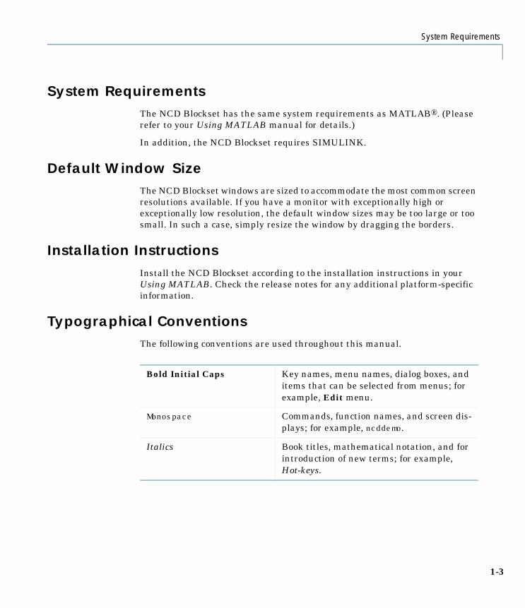
System RequirementsThe NCD Blockset has the same system requirements as MATLAB®. (Please refer to your Using MATLAB manual for details.)

In addition, the NCD Blockset requires SIMULINK.

Default Window SizeThe NCD Blockset windows are sized to accommodate the most common screen resolutions available. If you have a monitor with exceptionally high or exceptionally low resolution, the default window sizes may be too large or too small. In such a case, simply resize the window by dragging the borders.

Installation InstructionsInstall the NCD Blockset according to the installation instructions in your Using MATLAB. Check the release notes for any additional platform-specific information.

Typographical ConventionsThe following conventions are used throughout this manual.

Bold Initial Caps Key names, menu names, dialog boxes, and items that can be selected from menus; for example, Edit menu.

Monospace Commands, function names, and screen dis-plays; for example, ncddemo.

Italics Book titles, mathematical notation, and for introduction of new terms; for example, Hot-keys.

1-3

1 Introduction

1-4

2

Tutorial

2 Tutorial

To use the NCD Blockset effectively, you must first be comfortable with designing systems using SIMULINK. For more information on SIMULINK, consult your Using SIMULINK manual.

The pictures shown in this guide were generated either from a Macintosh IIci computer with a 4-bit grayscale monitor or a HIQ Personal Computer (running WindowsNT4.0) with a NOKIA Multigraph 445X monitor. If you use a different computer, your window borders and buttons may look different.

2-2

Quick Start

Quick StartIf you would like to get started using the NCD Blockset quickly, this section describes a short series of actions you can take to get going.

1 Make a model of your (nonlinear) system and controller using SIMULINK. Add input signals (e.g., steps, ramps, observed data) to the system for which you know what the desired output should look like.

2 Attach NCD blocks to the signals to be constrained. The SIMULINK system ncdblock contains the NCD block. To open the system, just type ncdblock at the MATLAB prompt.

3 In the MATLAB workspace, initialize the variables you want to tune with “a best first guess.”

4 Double-click on the NCD blocks in your system to bring up a constraint figure for each constrained output. Press the Help push button on the con-straint figure for general information on NCD Blockset functionality or select Hot-key help... from the Style menu. Double-clicking on an NCD block also updates its icon in your SIMULINK system; the icon now displays the port number assigned this NCD block.

5 Stretch, move, open, split, or toggle through constraints by using the Edit menu items, the mouse buttons, or the Hot-keys.

6 Open the Optimization Parameters dialog box by selecting Parameters... from the Optimization menu. Pick a discretization interval (try between one and two percent of the total time axis). Type in the Tunable Variables separating them by spaces or commas. For now, the default entries of the other dialog box fields should suffice. Press the Help push button on the Optimization Parameters dialog box for more information.

7 OPTIONAL: Open the Uncertain Variables dialog box by selecting Uncer-tainty ... from the Optimization menu. Uncertain variables should be ini-

2-3

2 Tutorial

tialized to their nominal values in the base workspace. Press the Help push button on the Uncertain Variables dialog box for more information.

8 OPTIONAL: Save the constraint data to a file using the Save ... submenu of the File menu. Constraints previously saved to a file can be retrieved using the Load ... submenu of the File menu.

9 Press the Start push button or select Start from the Optimization menu.

2-4

A Control Design Example

A Control Design ExampleThe NCD Blockset uses time domain constraint bounds to represent lower and upper bounds on response signals. Constraint bounds can be stretched, moved, split, or opened in a variety of ways, which are explained here and in Chapter 6. This section and the next section guide you through two examples of how you might perform control design and system identification using the NCD Blockset. In this section, we want to control a second order SISO system via integral action as shown below.

Specifically, the integral gain (Kint) should ensure that the closed loop system meets or exceeds the following performance specifications when we excite the system with a unit step input:

• A maximum 10 percent overshoot

• A maximum 10 second rise time

• A maximum 30 second settling time

Because of the actuator limits and system transport delay, standard linear control design techniques may not yield reliable results.

NCD StartupThe SIMULINK system ncdtut1 contains the system shown above. You can open the system by typing ncdtut1 at the MATLAB prompt. The system was

2-5

2 Tutorial

created just as any other SIMULINK system; you need not remodel any of your present SIMULINK systems to use the NCD Blockset. You need simply to

• Attach an NCD block to all signals you want to constrain. In ncdtut1, we attach an NCD block (square block with a step response display) to the plant output.

• Add input signals to the system for which you know what the output should look like. In ncdtut1, we input a step to the system since we know the desired step response characteristics of the system.

• Adjust the simulation Start time and Stop time appropriately. In ncdtut1, the step response should settle within 30 seconds, so making the simulation run to 50 seconds allows the step to go to completion. Since the NCD optimi-zation calls for many simulations of the system, you should make the simu-lation time as short as possible, but long enough to show dynamics of interest. You can change the Start time and Stop time through the SIMULINK Simulation parameters dialog created by selecting Parame-ters... from the Simulation menu.

Before continuing, MATLAB variables in the SIMULINK model must be initialized. At the MATLAB prompt, type

zeta = 1;w0 = 1;Kint = 0.3;

We choose the initial value for Kint after plotting step responses of the linearized system for a few values of Kint.

Adjusting ConstraintsTo open the NCD Blockset constraint window, double-click on the NCD block. As shown below, the title of the constraint figure includes the name of the SIMULINK system in which the NCD block resides (in this case the system ncdtut1). The constraint window contains a response versus time axis, a control panel, and default upper and lower constraint bounds. An NCD menu

2-6


bar appears either at the top of the constraint figure or at the top of your screen depending upon what type of computer system you have.

The constraint window appears in a default location and default size. You can move the constraint window to a more convenient location or make it larger or smaller. The thickness of the constraint bounds holds no significance to the optimization formulated; it merely provides visual cues defining where constraint bounds can be clicked-and-dragged.

The lower and upper constraint bounds define a channel between which the signal response should fall. The default constraints effectively define a rise time of five seconds and a settling time of 15 seconds. These bounds must change to reflect the performance requirements proposed in the beginning of this section. To adjust the rise time constraint, position the mouse over the vertical line separating the lower bound constraint that ends at five seconds and the lower bound constraint that begins at five seconds. Press and hold

2-7

2 Tutorial

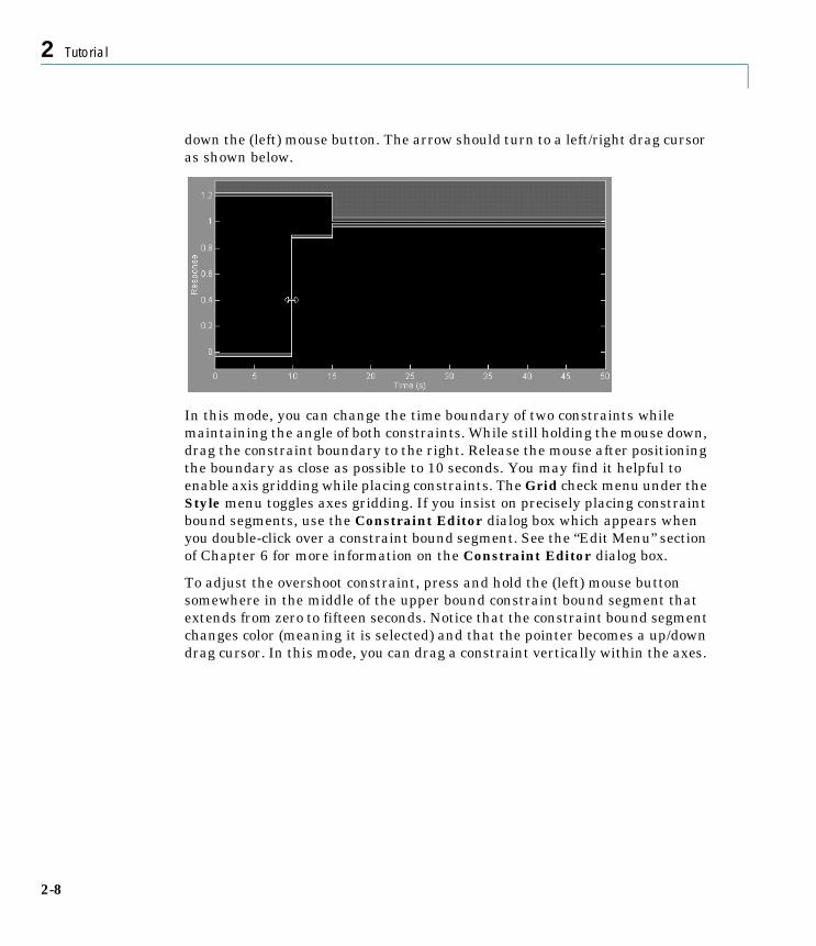
down the (left) mouse button. The arrow should turn to a left/right drag cursor as shown below.

In this mode, you can change the time boundary of two constraints while maintaining the angle of both constraints. While still holding the mouse down, drag the constraint boundary to the right. Release the mouse after positioning the boundary as close as possible to 10 seconds. You may find it helpful to enable axis gridding while placing constraints. The Grid check menu under the Style menu toggles axes gridding. If you insist on precisely placing constraint bound segments, use the Constraint Editor dialog box which appears when you double-click over a constraint bound segment. See the “Edit Menu” section of Chapter 6 for more information on the Constraint Editor dialog box.

To adjust the overshoot constraint, press and hold the (left) mouse button somewhere in the middle of the upper bound constraint bound segment that extends from zero to fifteen seconds. Notice that the constraint bound segment changes color (meaning it is selected) and that the pointer becomes a up/down drag cursor. In this mode, you can drag a constraint vertically within the axes.

2-8


While still holding the mouse button down, drag the constraint until its lower boundary is at a height of 1.1 as shown below.

Finally, the settling time constraints require adjustment. Position the mouse button just within the left edge of the upper bound constraint extending from 15 to 50 seconds. Press and hold down the (left) mouse button and notice that the constraint becomes selected and that pointer changes to a fleur. In this mode, you can stretch the end of the constraint at any angle. While still holding the mouse button down, drag the constraint so that the settling time constraint begins at 30 seconds. Consider enabling the snapping option if you have difficulty releasing the constraint so that it exactly ends up being horizontal. The Snap check menu under the Style menu toggles constraint bound snapping. With snapping enabled any dragged constraint end snaps to an angle that is a multiple of 22.5 degrees. Adjust the lower bound constraint so

2-9

2 Tutorial

that it too defines a 30 second settling time constraint. The constraint figure should now look the one shown below.

Before beginning the optimization, you must tell the NCD Blockset which variables are tunable for optimization. Open the Optimization Parameters dialog box by selecting Parameters... from the Optimization menu. Simply type Kint into the Tunable Variables: editable text field as shown below.

If more than one tunable variable exists, type in the variable names separated by spaces. You might also want to change the discretization interval. This

2-10


number relates to the number of constraints generated by the optimization; the larger the discretization interval, the fewer constraints generated but the less rigorous the optimization. Typical discretization intervals range between one and two percent of the total simulation time. For more technical information on how the discretization interval affects the optimization problem formulated by the NCD Blockset, see the Appendix.

Running the OptimizationAfter adjusting the constraint bounds in the NCD constraint figure and declaring the tunable variables using the Optimization Parameters dialog box, you are ready to begin the optimization. You can start an optimization by pressing the Start button on the NCD Control panel or by selecting Start from the Optimization menu.

When you start the optimization, the NCD Blockset automatically converts the constraint bound data and tunable variable information into a constrained optimization problem. It then invokes the Optimization Toolbox routine constr. The routine adjusts the tunable variables in an attempt to better achieve the constraints on system signals defined by the NCD main interface. The routine constr solves constrained optimization problems using a sequential quadratic programming (SQP) algorithm and quasi-Newton gradient search techniques. See the section “Solving the Optimization Problem” for more information on how the NCD Blockset uses constr to optimize the tunable variables. In short, the optimization problem formulated by the NCD Blockset minimizes the maximum constraint violation. The number of iterations necessary for the optimization to converge and the final values of the tunable variables depend not only on the specific problem but also on the computer system.

2-11

2 Tutorial

For the problem posed above, the output on a PC running WindowNT4.0 is as follows:

To inspect the new value of the tunable variable, simply type the variable name at the MATLAB prompt:

During optimization, the NCD Blockset first displays information about plant uncertainty, a topic discussed in the next subsection. Next the blockset displays information regarding the number of constraints per simulation and simulations conducted. To determine the total number of constraints to be met, multiply the constraints generated per simulation by the number of simulation per cost function call. Information regarding the progress of the optimization follows.

The first column of output shows the total number of cost function calls. To calculate the total number of simulations conducted, multiply the number of function calls by the number of simulations per cost function call. The second column (max{g}) shows the maximum (weighted) constraint violation (i.e., the

Processing uncertainty information.Uncertainty turned off.Setting up call to optimization routine.Start time: 0 Stop time: 50.There are 205 constraints to be met in each simulation.There are 1 tunable variables.There are 1 simulations per cost function call.Creating simulink model NCDmodel for gradients...Donef-COUNT MAX{g} STEP Procedures 3 0.182918 1 6 0.0404898 1 Hessian modified twice 9 -0.00560194 1 Hessian modified twice 12 -0.00561533 1 Hessian modified twice 13 -0.00567585 1 Hessian modified twice Optimization Converged SuccessfullyActive Constraints: 124 165

» Kint

Kint =

0.1867

2-12


cost function). This number should decrease during the optimization. When max{g} becomes negative, all constraints have been met. In the case above, a negative max{g} shows that all constraints were met after the ninth function call and the optimization then proceeded to overachieve. The third column (STEP) displays the step size used by the line search algorithm. The last column shows special messages related to the quadratic programming subproblem. If the termination criteria are met, the optimization ends with the message Optimization Converged Successfully. Note that this does not imply that all constraints have been met.

Finally, the optimization displays an encoded list of the active constraints (i.e., which constraints prohibit further decrease in the cost function). For detailed information on the optimization algorithm, see the Appendix. The command window display can be disabled by unchecking the Display optimization information check box on the Optimization Parameters dialog box.

When the NCD Blockset begins the optimization, it plots the initial response in white. To view the (initial) response without beginning the optimization, select Initial response from the Options menu. Viewing the initial response may help you define better constraint bounds. At each iteration the optimization plots an intermediate response. You can terminate the optimization at any time and recover intermediate results by pressing the Stop push button or selecting Stop from the Optimization menu.

Because of different numerical precision, the results of the optimization may differ slightly across different platforms.

Adding UncertaintyIn your particular problem, a precise plant model may not be known. Instead you know what the nominal plant should be and have some idea of the uncertainty inherent in various components of the plant. For example, assume that the plant parameter zeta varies 5% about its nominal value and w0 varies between 0.7 and 1.45.

The NCD Blockset allows you to design controllers to meet performance objectives in the face of this uncertainty. Just open the Uncertain Variables dialog box by selecting Uncertainty... from the Optimization menu and type in the names of the uncertain variables and their ranges as shown on the next page. The NCD Blockset automatically incorporates this uncertainty into the optimization.

2-13

2 Tutorial

The Uncertain Variables: editable text field expects you to supply a list of variable names. You can separate the variable names by spaces or commas. The optional lower and upper bound editable text fields accept variable names, numbers, and expressions. Expressions can contain, in addition to numbers, variables available in the MATLAB base workspace.

Notice that by default the NCD Blockset only constrains the nominal plant during optimization. To constrain the lower or upper bound plant during optimization, check the appropriate check box. A further option allows you to constrain randomly generated plants between the upper and lower bound plants. Simply enter the number of random plants you would like to constrain into the Number of Monte Carlo simulations: editable text field and check the Constrain Monte Carlo simulations check box. A status line tells you how many simulations are performed during each call to the cost function. In the figure above, notice that we constrain only the upper and lower bound simulations for a total of two simulations per cost function call.

Although constraining more plants results in more robust control design, it adds to the optimization time. We recommend that you constrain as few plants

2-14


as possible during optimization and use the Monte Carlo option mostly for analysis purposes. For example, constrain only the upper and lower bound plants during optimization. Once the optimization terminates, simply inspect the system response for a number of random plants by selecting Initial response... from the Options menu after constraining a number of Monte Carlo simulations using the Uncertain Variables dialog box. If this analysis shows the design to be unsatisfactory, then consider optimizing with the Monte Carlo option enabled.

With the Uncertain Variables dialog box filled in as above, start the optimization again. Notice that now the NCD Blockset draws two initial plots and updates two others. The plots show the output of the upper and lower bound plants. In general, the NCD Blockset draws a plot for each plant constrained. Note too that the output to the command window now shows each cost function call conducting two simulations.

If you want to erase the plots on an NCD constraint figure, select Delete plots from the Edit menu.

2-15

2 Tutorial

A System Identification ProblemThe next example, ncdtut2, shows one technique for using the NCD Blockset to perform closed loop system identification. Specifically, we want to estimate the mass and length of the pendulum in a variation of the popular inverted pendulum problem. The physical system contains a cylindrical metal rod attached to a motor driven cart to allow for rotation about only one axis. We mount the cart on a linear track to create a stabilizable problem as shown below.

The rod initially has a mass of 0.21kg and a length of 0.61m and is stabilized via LQR control. The Appendix explains both the equations of motion for the system and the design of the LQR controller.

With the LQR controller stabilizing the system, we stick a clay ball to the top of the rod, thus changing the effective pendulum mass and length. Now we want to estimate this new pendulum mass and length.

NCD StartupThe SIMULINK system ncdtut2 contains a block diagram representation of the experiment described above. You can open the system by typing ncdtut2 at the MATLAB prompt.

2-16

A System Identification Problem

Notice that in addition to the inherent nonlinearities of the system equations, limits on the voltage applied to the motor result in an actuation saturation constraint of one Newton. Notice that the system contains two NCD blocks as we use both pendulum angle and cart position signals to perform identification. The basic approach to performing system identification using the NCD Blockset involves constraining the error signals. To form error signals, use the From Workspace block to import observed data into your system and then subtract the simulated signal.

Before continuing, you must define some system parameters and load the observed data. At the MATLAB command line, type

penddata % Loads T, U, yHat, ThetaHat, g, and Mcl = 0.61/2; % Distance to center of mass of pendulum (m)

% i.e., one–half length of pendulumm = 0.21; % Mass of pendulum (kg)

In the real world system, sensors measure only cart position and pendulum angle and we calculate the velocities using finite difference estimators. Here we ignore such considerations and assume full state feedback. Also in the real

2-17

2 Tutorial

world, the measured and input signals contain noise. Here we simply generated the observed output signals (yHat and ThetaHat) by simulating the system at the solution point (m=0.3 and l=0.32). We did not add noise.

We apply a modified chirp signal, U, to the system. We find such signals useful in system ID applications because they contain contributions from a specified frequency range [1]. The signal U possesses (nearly) uniform frequency components between 1Hz and 10Hz. A time response plot and power spectral analysis of the signal appear below.

We use gain blocks to magnify and normalize the error signals before passing them to the NCD block. Note that the position error is magnified Gy = 200 times, whereas the angle error is magnified by a factor Gt = 100. Alternatively, you could have weighted the signals using the Constraint Editor dialog box as described in the “Edit Menu” section of Chapter 6. We suggest the convention of using gain blocks to normalize signals (i.e., weighting all constraint segments of an output) and constraint segment weighting for weighting one constraint segment of the same output relative to another.

0 0.5 1 1.5 2 2.5 3 3.5 4 4.5 5-0.1

-0.05

0

0.05

0.1

Time (s)

Inpu

t

Excitation Signal Time Response Plot

100

101

10-6

10-4

10-2

Frequency (Hz)

Mag

nitu

de

Power Spectrum of Excitation Signal

2-18


Adjusting ConstraintsWith the error signals as defined above, we simply want to drive them as close to zero as possible. Thus we intend to design constraint bars that merely bracket zero. Since the errors signals have been magnified via the gain blocks, we constrain both (magnified) error responses to within ±1 of zero. You might define these constraints in a number of ways:

Method 1: Click and drag constraints: First open the NCD constraint figures as in the previous section by double-clicking on the NCD blocks. Then simply click and drag constraint bound segments around as in the previous section.

Method 2: Use the Constraint Editor dialog box: To use the Constraint Editor, first open the NCD constraint figures as in the previous section by double-clicking on the NCD blocks. Then open the Constraint Editor dialog box by clicking the right mouse button on a constraint bound segment. If you opened the editor on a lower bound segment, enter[0 -1 5 -1] into the Position editor [x1 y1 x2 y2]: editable text field. Otherwise, you have opened the editor on an upped bound constraint, therefore, type [0 1 5 1] into the editable text field.

Since the lower constraint bounds are now outside the default y-axis range, open the Y-axis Range dialog box and change the Y-axes limits to [-1.5 1.5] on both the constraint figures. You can open the Y-axes Range dialog box by selecting Y-Axis... from the Options menu. For more information on the Y-axis Range dialog box, see the “Options Menu” section of Chapter 6.

When you open a constraint figure by double clicking on an NCD block, the global variable ncdStruct is created and initialized as a structure with various fields. The lower bound information is stored in ncdStruct.CnstrLB, the upper bounds in ncdStruct. CnstrUB, and the axes range information saved in ncdStruct.RngLmts. The data you input into the Constraint Editor and the Y-axes Range dialog boxes gets saved into the these fields of ncdStruct, and you can see the format in which the lower bound information is stored by typingncdStruct.CnstrLB at the MATLAB prompt. See the Appendix for more information regarding these variables and other data fields of ncdStruct.

Though the ncdStruct is available to you in the workspace, we strongly urge you not to modify it directly. We mention this at this point so that you aware that the NCD Blockset does create this global variable in your MATLAB workspace, and typing clear or clear global during an NCD session would require closing down all constraint windows and beginning the session anew.

2-19

2 Tutorial

Before starting the optimization, you must tell the NCD Blockset which parameters are tunable for optimization. Open the Optimization Parameters dialog box by selecting Parameters... from the Optimization menu of either constraint figure. Input changes to the dialog box’s editable text fields to make the dialog box look like the one below.

2-20


Running the OptimizationAfter adjusting the constraints and defining tunable variables, start the optimization by pressing the Start button on the NCD Control panel or by selecting Start from the Optimization menu. For the problem posed above, a PC running WindowsNT4.0 outputs:

Because of different numerical precision, the results of the optimization may differ slightly across different platforms. The constraint figures on the next page show the initial and final response plots for the cart position and pendulum angle error signals.

Processing uncertainty information.Uncertainty turned off.Setting up call to optimization routine.Start time: 0 Stop time: 5.There are 404 constraints to be met in each simulation.There are 2 tunable variables.There are 1 simulations per cost function call.Creating simulink model NCDmodel for gradients...Donef-COUNT MAX{g} STEP Procedures 5 0.466256 1 10 -0.421419 1 Hessian modified 15 -0.392145 1 20 -0.477709 1 25 -0.478421 1 Hessian modified twice 30 -0.473284 1 Hessian modified twice 35 -0.473988 1 Hessian modified twice 44 -0.473985 0.0625 Hessian modified twice 51 -0.474014 0.25 Hessian modified 60 -0.474371 0.0625 Hessian modified twice 93 -0.474371 -3.73e-009 Hessian modified twice 126 -0.474371 -3.73e-009 Hessian modified twice 159 -0.474371 -3.73e-009 Hessian modified twice 164 -0.473248 1 Hessian modified twice 165 -0.477089 1 Hessian modified twice Optimization Converged SuccessfullyActive Constraints: 54

2-21

2 Tutorial

2-22


You may want to investigate how incorporating noise into the observed data affects the optimization. To do this simply

• Reinitialize the tunable variables to their initial values: m = 0.21;l = 0.61/2;

• Add random noise to the observed data vectors:yHat = yHat + 0.001*rand(size(yHat));ThetaHat = Thetahat + 0.001*rand(size(ThetaHat));

• Restart the optimization.

The optimization still converges to the known solution, but it takes more iterations to do so.

Due to the design of the experiment, you know that the solution mass and length are larger than the initial mass and length (re: a clay ball is stuck to the end of the pendulum). Thus, you can constrain the lower bounds of the tunable parameters using the Tunable Parameters dialog box. In general, add such constraints whenever possible since the added information allows the optimization to make better decisions about how to search the parameter space.

2-23

2 Tutorial

Solving the Optimization ProblemThe NCD Blockset transforms the constraints and simulated system output into an optimization problem of the form

where the boldface characters denote vectors. Variable x is a vectorization of the tunable variables while xl and xu are vectorizations of the lower and upper bounds on the tunable variables. The vector g(x) is a vectorization of the constraint bound error and w is a vectorization of weightings on the constraints. The scalar γ imposes an element of slackness into the problem, which otherwise imposes that the goals be rigidly met (See the Appendix for more information).

Basically, the NCD Blockset attempts to minimize the maximum (weighted) constraint error. The NCD Blockset generates constraint errors at equally spaced time points (with spacing given by the Discretization interval defined in the Tunable Parameters dialog box) beginning at the simulation start time and ending at the simulation stop time. For upper bound constraints, we define the constraint error as the difference between the constraint boundary and the simulated output. For lower bound constraints, we define the constraint error as the difference between the simulated output and the constraint boundary.

This type of optimization problem is solved in the Optimization Toolbox routine constr. The routine uses a Sequential Quadratic Programming (SQP) method which solves a Quadratic Programming (QP) problem at each iteration. At each iteration, the routine updates an estimate of the Hessian of the Lagrangian. The line search is performed using a merit function. The routine uses an active set strategy for solving the QP subproblem.

For more information on the algorithm implemented by constr, see the Appendix or the Optimization Toolbox User’s Guide.

min γx γ, s.t.

g x⟨ ⟩ wγ– 0≤xl x xu≤ ≤

2-24

NCD Blockset Command Line Interaction

NCD Blockset Command Line InteractionYou can conduct an NCD Blockset session from the command line without using NCD constraint figures or even the NCD block. We expect, however, that you will prefer the convenience and efficiency of the constraint figure. Without the constraint figure, constraint bounds are difficult to visualize. Also during optimization, you can watch the cost function decrease, but you cannot observe the evolution of the system response. Thus you cannot tell which constraints prohibit further decrease in the cost function.

Before beginning the optimization, you must declare ncdStruct as global and initialize the fields of this structure. See the Appendix for details about the fields in ncdStruct. You can use the script file ncdglob.m to define ncdStruct as global and set up its fields. If you have already saved a set of constraints (by selecting Save... from the NCD constraint figure File menu), you can declare and define the necessary global variables by typing

ncdglob; load myfile

at the MATLAB prompt, where myfile is the file to which you saved your constraints.

Once you declare and define the necessary global variables, you can start the optimization by typing

nlinopt('sfunc')

at the MATLAB prompt where sfunc is the name of your SIMULINK system. If ncdStruct.OptmOptns(1) = 1, the NCD Blockset displays optimization information in the command window. The rest of this section describes which fields in ncdStruct need to be defined in order to conduct NCD sessions from the MATLAB command line.

The NCD block is a masked outport block, which calls the constraint figure creation routine optblock when you double-click on it. Since nlinopt directly looks for these masked outport blocks in your model, the constraint figures need not be open to start the optimization routine. However, you must initialize the fields in ncdStruct for nlinopt to work. Specifically, you must initialize the following fields: ncdStruct.CnstrLB, ncdStruct.CnstrUB,ncdStruct.TvarStr, ncdStruct.Tdelta, ncdStruct.CostFlag,ncdStruct.GradFlag,ncdStruct.RngLmts, and ncdStruct.SysName. Consult the Appendix for more information about these variables, and see the demo initialization scripts

2-25

2 Tutorial

ncd1init, ncd2init, ncd3init, and ncd4init for more examples on how to define these variables. If you want to perform an optimization with uncertainty in your plant dynamics, you must further initialize and the following variables: ncdStruct.UvarStr, ncdStruct.UvlbStr, ncdStruct.UvubStr, ncdStruct.NumMC, and ncdStruct.PlntON. Again, the Appendix and demo initialization files can help you understand how to use and define these variables.

NCD and the SIMULINK AcceleratorThe NCD Blockset works automatically and seamlessly with the SIMULINK Accelerator. If you have the SIMULINK Accelerator, simply check Accelerate on your SIMULINK system Simulation menu and the NCD Blockset will run with the C code generated by the SIMULINK Accelerator. Because the majority of NCD Blockset optimization time is spent conducting simulations, using the SIMULINK Accelerator could greatly decrease the amount of time it takes to perform an optimization. To get the most speed from the SIMULINK Accelerator, you should close all Scope blocks and either remove M-file function blocks or replace them with Fcn blocks.

Printing a NCD Blockset Constraint FigureSelect Print from the File menu on the NCD Blockset constraint figures to send hardcopies of figures to the printer. The Print menu item brings up a dialog box and lets you set the print options, before sending the figure to the printer. Consult your Using MATLAB manual for more information.

Since the NCD Blockset control panel and menu bar are separate platform dependent window objects, they do not appear in the printed hardcopy. Constraint bars do appear in the printed hardcopy. If you want the NCD control panel and menu bar to appear in your hardcopy, use the screen capture technique of your choice.

References[1] Weizheng Wang, Modeling Scheme for Vehicle Longitudinal Control, CDC, Tuscon, 1992, pp. 549-54.

2-26

3
Problem Formulation

3 Problem Formulation

The NCD Blockset can aid in the design and identification of complex control systems (including gain scheduled and multimode control and repeated parameter problems). Such problems are found in everyday engineering practice but little theory addresses them.

This chapter provides brief descriptions of how various problems not discussed in Chapters 2 and 4 can be formulated and solved using the NCD Blockset.

3-2

Actuation Limits vs State Constraints (Physical vs Design Constraints)

Actuation Limits vs State Constraints (Physical vs Design Constraints)

To incorporate actuator limits and other physical constraints using the NCD Blockset, simply use SIMULINK’s Saturation block. You do not need to attach an NCD block and define NCD constraints for such signals since the physics of the system guarantees that the signal cannot exceed the limits. For example, consider the pendulum examples of Chapters 2 and 4 and notice the Saturation block after the Klqr gain block. This Saturation block models the actuator limits of the controller. The power electronics of the controller limit the voltage supplied to the motor driving the cart. This voltage limit in turn limits the amount of force applied by the cart to ±1 Newton.

On the other hand, to incorporate design constraints, use the NCD block to constrain a state or signal. In the inverted pendulum example, although the pendulum angle physically can exceed ±0.2 radians, we require that an acceptable controller does not allow the pendulum to exceed such a constraint.

Minimizing Integrated Positive Signals (Control Energy)Again, such signals can be considered design constraints. If the signal does not exist naturally in the system, you can model it using the Abs and Integrator blocks in SIMULINK. Even though we do not typically view such constraints as point-by-point constraints (i.e., intermediate time values of the signal are of no interest), the design constraint analogy still holds because over time, the integral increases. Thus you know that the signal can never have a value at its final time smaller than at any intermediate time. Also, although many problems concerning the minimization of integrated signals extend to an infinite time horizon (the NCD Blockset is practical only over shorter time horizons), the signals typically begin converging to their infinite time horizon limit in a finite time (over which the NCD Blockset can practically be applied).

Before using the NCD Blockset to minimize integrated signals, consider whether such a design goal really makes sense to you. Much modern control theory considers the minimization of integrated positive signals, partly because such signals possess some relation to the real world and partly because such problems possess well known closed-form solutions. For something such as simple motor actuation, you may instead want to incorporate actuator saturation using a Saturation or Limited Integrator block. On the other hand, for something such as jet engine control, minimizing total fuel consumption (an integrated positive signal) may be necessary.

3-3


Noise InputsNo noise should be included in the SIMULINK model during optimization. Including noise in the system while optimizing effectively introduces inconsistency into the problem formulation and may cause the optimization to converge more slowly or even fail to converge altogether. Modern control theory techniques often define noise terms in their problem formulation as approximations to plant, actuator, or sensor uncertainty. In other cases, modern control theory effectively uses the noise covariance matrices as tweakable design handles. Using the NCD Blockset, you can design controllers while directly incorporating uncertainty into plant, actuator, or sensor dynamics by using the Uncertain Variables dialog box. Instead of framing your control design in terms of minimizing various norms of weighted transfer functions, and tuning your response by tweaking the weights, the NCD Blockset utilizes the time domain constraint bound paradigm.

Of course, noisy measurements do exist in the real world, and you must take such noise into consideration when you do your design. In the general case, you should simply inspect the system performance with noise added after optimizing. If you must include noise in your system during optimization, follow these suggestions.

• For continuous systems, use the Band Limited White Noise block (found in the SIMULINK sources library), a fixed time step integration (set the min-imum and maximum time step to be equal), and a constant seed for the noise.

• For discrete systems, use the White Noise block (found in the SIMULINK Sources library) with a constant seed for the noise.

Increasing the noise in a system often forces you to design more conservative control to maintain system stability. If including noise in your system produces unacceptable instability, consider changing your NCD constraint bounds to allow less overshoot and longer rise times and settling times. If this results in unacceptable system performance, consider options that decrease sensor noise.

3-4

Tracking

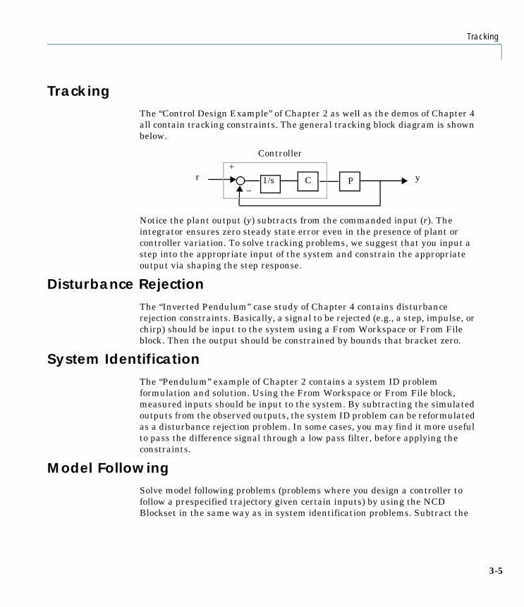
TrackingThe “Control Design Example” of Chapter 2 as well as the demos of Chapter 4 all contain tracking constraints. The general tracking block diagram is shown below.

Notice the plant output (y) subtracts from the commanded input (r). The integrator ensures zero steady state error even in the presence of plant or controller variation. To solve tracking problems, we suggest that you input a step into the appropriate input of the system and constrain the appropriate output via shaping the step response.

Disturbance RejectionThe “Inverted Pendulum” case study of Chapter 4 contains disturbance rejection constraints. Basically, a signal to be rejected (e.g., a step, impulse, or chirp) should be input to the system using a From Workspace or From File block. Then the output should be constrained by bounds that bracket zero.

System IdentificationThe “Pendulum” example of Chapter 2 contains a system ID problem formulation and solution. Using the From Workspace or From File block, measured inputs should be input to the system. By subtracting the simulated outputs from the observed outputs, the system ID problem can be reformulated as a disturbance rejection problem. In some cases, you may find it more useful to pass the difference signal through a low pass filter, before applying the constraints.

Model FollowingSolve model following problems (problems where you design a controller to follow a prespecified trajectory given certain inputs) by using the NCD Blockset in the same way as in system identification problems. Subtract the

PC1/s yr+

_

Controller

3-5


simulated outputs from the desired trajectories and constrain these signals as you would a system identification or disturbance rejection problem.

Adaptive ControlDesign adaptive controllers using the NCD Blockset as you would any other controller. You can tune forgetting factors and sampling times, but not model order. Choosing model order is an integer optimization problem that the NCD Blockset (which calls the routine constr) cannot solve.

MIMO SystemsTo design MIMO controllers or perform MIMO system ID, attach an NCD block to all signals to be constrained and design constraints for each signal over independent time intervals. The “MIMO PI Controller” example of Chapter 4 shows how to design constraints for a two-input, two-output tracking problem with cross-channel decoupling.

Multimode ControlMultimode control concerns designing one or more controllers for a plant as it transitions over a wide range of dynamic behavior. Typically you make a linear approximation of the plant at a number of operating points (plant conditions) and then generate a controller for each operating point. The plant models at the operating points often have different dynamic order and the controllers for each operating point generally have different structure and/or order. Multimode control also considers the design of the logic (supervisory control), which switches between the various controllers designed for each operating point. To model a multimode controller in SIMULINK, use switch blocks to toggle among the various plant and controller models according to the operating conditions of the plant. Use logic blocks (from the extrlog directory) to create the supervisory control that manages the switches.

The NCD Blockset allows you to design multimode controllers and simplifies the process in two ways: by providing a means to tune the switching logic and by decreasing the number of controllers you need to generate. As with other problems, you can design your controller using the actual nonlinear plant model instead of a number of operating point linear approximations. Not only does this reduce the amount of verification that you must perform once the optimization produces results, but it also allows you to tune the switching logic parameters. In the case of multimode control, the ability to design nonlinear

3-6

Gain Scheduling

controllers may not only create the possibility for improved performance over linear control, but may decrease the number of controller you must generate since a single nonlinear controller may be applicable to more than one operating point.

Gain SchedulingGain scheduling problems may be considered a subset of multimode control problems where the controller order and structure remain consistent over all operating points.

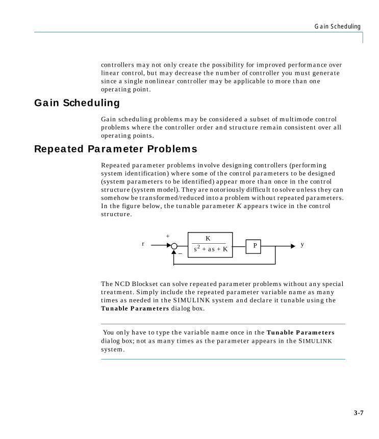
Repeated Parameter ProblemsRepeated parameter problems involve designing controllers (performing system identification) where some of the control parameters to be designed (system parameters to be identified) appear more than once in the control structure (system model). They are notoriously difficult to solve unless they can somehow be transformed/reduced into a problem without repeated parameters. In the figure below, the tunable parameter K appears twice in the control structure.

The NCD Blockset can solve repeated parameter problems without any special treatment. Simply include the repeated parameter variable name as many times as needed in the SIMULINK system and declare it tunable using the Tunable Parameters dialog box.

You only have to type the variable name once in the Tunable Parameters dialog box; not as many times as the parameter appears in the SIMULINK system.

P yr+

_

K__________s2 + as + K

3-7


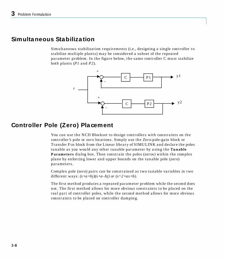
Simultaneous StabilizationSimultaneous stabilization requirements (i.e., designing a single controller to stabilize multiple plants) may be considered a subset of the repeated parameter problem. In the figure below, the same controller C must stabilize both plants (P1 and P2).

Controller Pole (Zero) PlacementYou can use the NCD Blockset to design controllers with constraints on the controller’s pole or zero locations. Simply use the Zero-pole-gain block or Transfer Fcn block from the Linear library of SIMULINK and declare the poles tunable as you would any other tunable parameter by using the Tunable Parameters dialog box. Then constrain the poles (zeros) within the complex plane by enforcing lower and upper bounds on the tunable pole (zero) parameters.

Complex pole (zero) pairs can be constrained as two tunable variables in two different ways: (s+a+bj)(s+a–bj) or (s^2+as+b).

The first method produces a repeated parameter problem while the second does not. The first method allows for more obvious constraints to be placed on the real part of controller poles, while the second method allows for more obvious constraints to be placed on controller damping.

P2C y2+

_

P1C y1

r

+

_

3-8

Strong Stabilization

Strong StabilizationStrong stabilization requirements (i.e., designing a stable controller to stabilize a system) may be considered a subset of the pole placement problem. Specifically, all poles of the controller are constrained to lie in the left half plane.

For real poles (e.g., s+a), simply enforce a lower bound of zero on the tunable pole (a) using the Lower Bound: editable text field in the Tunable Variables dialog box. Complex pole pairs defined as either (s+a+bj)(s+a–bj) or (s^2+as+b) should include the lower bound a,b>0.

3-9


3-10

4

Case Studies

4 Case Studies

To provide extended examples of use, this chapter presents four benchmark problems, which are contained separately in the SIMULINK systems ncddemo1, ncddemo2, ncddemo3, and ncddemo4. All four are contained in the SIMULINK system ncddemo. The problems increase in sophistication from ncddemo1 to ncddemo4.

4-2

Case Study 1: PID Controller

Case Study 1: PID ControllerIn the first control design problem, ncddemo1, we model the nominal plant as the third-order SISO transfer function.

where a2 = 43 and a1 = 3 nominally with rate limit (±0.8) and saturation (±2) nonlinearities. Additionally, because of design tolerances, actual plant dynamics exhibit significant variation from the nominal. Specifically, the denominator coefficient a2 varies between 40 and 50 and the coefficient a1 varies between one-half and 1.5 time its nominal value of 3.

Problem DefinitionWe want to design a PID controller for the system so that the closed loop system meets the following tracking specifications:

• Maximum overshoot of 20%

• Maximum 10 seconds rise time

• Maximum 30 seconds settling time

Further, we want the closed loop response to be robust to the uncertainty in the plant dynamics.

G s⟨ ⟩ 1.5

50s3 a2s2 a1s 1+ + +----------------------------------------------------------=

4-3

4 Case Studies

Problem SetupThe SIMULINK system ncddemo1 contains the plant and control structure as shown below. To open the system, type ncddemo1 at the MATLAB prompt or double-click on the NCD Demo 1 block in the SIMULINK system ncddemo. Notice the rate and saturation nonlinearities included in the plant model. A step input drives the system. The NCD block attaches to the plant output since it is the signal to be constrained. Inspecting the System’s Parameters dialog box shows that each simulation lasts 100 seconds.

Double-click on the block ncd1init to initialize the tunable and uncertain variables. The uncertain variables, a2 and a1, are initialized to their nominal values of 40 and 3 respectively. The tunable parameters, Kp, Ki, and Kd initialize to 0.63, 0.0504, and 1.9688 respectively. These values result from using the Ziegler-Nichols method for tuning PID controllers [1, Ch.3]. The Ziegler-Nichols method for tuning PID controllers can be summarized as follows:

• Set the integral and derivative gains to zero and increase the proportional gain until the system just becomes unstable.

• Define this gain to be Ku and measure the period of oscillation, Pu.

• Set Kp = 3*Ku/5, Ki = 6*Ku/(5*Pu), and Kd = 3*Ku*Pu/40.

Double-clicking on the ncd1init block also defines the time domain response constraints for this demonstration. Double-click on the NCD block to open the NCD Blockset constraint figure and display the constraints. The lower and upper constraint bounds effectively define overshoot, rise time, and settling time constraints.

Problem SolutionBefore starting the optimization, open the Optimization Parameters dialog box by selecting Parameters... from the Optimization menu and notice how the Tunable Variables are defined. Also open the Uncertain Variables dialog box by selecting Uncertainty... from the Optimization menu. Notice how the uncertainty in the parameters a2 and a1 is defined and also note that the optimization constrains only the nominal plant.

Press the Start button, select Start from the Optimization menu, or hold down the accelerator key and press t to start the optimization. Watch the response evolve and improve during the optimization. The optimization time, cost

4-4

Case Study 1: PID Controller

function evolution, and final values for the tunable variables may differ for different computers. However, the optimization should produce a controller that meets all the constraints.

Now return to the Uncertain Variables dialog box and constrain the upper and lower bound plants. Press Start to begin optimizing with uncertainty. You may find that all the constraints cannot now be met, but the displayed output shows a maximum constraint violation of less than 0.01. Considering the degree of uncertainty in the plant dynamics, such a result is still impressive.

You can experiment if you want, moving the constraint bounds in an attempt to achieve even better system performance. For example, decrease the rise time or lower the overshoot constraints.

4-5

4 Case Studies

Case Study 2: LQR with Feedforward ControllerThe second problem, ncddemo2, requires the Control System Toolbox as it is an extension of problems found in the SIMULINK demo file lqgdemos. We model the SISO plant as a fourth-order linear state-space system augmented with saturation (±5) and rate limit (±10) nonlinearities. The equations

define the nominal plant. For illustration purposes, we allow the plant A matrix to vary between one half and twice its nominal value.

Problem DefinitionUsing LQG/LTR techniques, we design a Kalman state estimator and regulator gain (K) for the linear system. Next we add an integrator to guarantee zero steady state error. To achieve increased response time, we add a feedforward gain (FF). In the SIMULINK demo system lqgopt, the control parameters K and FF are tuned via an adhoc least squares method. We tune these parameters here using the NCD Blockset.

Specifically, we want to tune the control parameters K and FF such that the closed loop system meets the following tracking specifications:

• Maximum overshoot of 20%

• Maximum one second rise time

• Maximum three second settling time


Problem SetupThe SIMULINK system ncddemo2 contains the plant and control structure shown below. To open the system, type ncddemo2 at the MATLAB prompt or double-click on the NCD Demo 2 block in the SIMULINK system ncddemo.

y 1.7786– 1.1390 0 1.0294– x Cx= =

x·1.0285– 0.9853 0.9413– 0.09271.2903– 1.0957– 2.8689 4.79500.1871 3.8184– 2.0788– 0.9781–

0.4069 4.1636– 2.5407 1.4236–

x

06.6389

00

u+ Ax Bu+= =

4-6

Case Study 2: LQR with Feedforward Controller

Notice the rate limit (±10) and saturation (±5) nonlinearities included in the plant model. Using the From Workspace block, we input a step that transitions from zero to one at one second. The NCD block attaches to the plant output since it is the signal to be constrained. Inspecting the System’s Parameters dialog box shows that each simulation lasts 10 seconds.

Double-click on the block ncd2init to initialize the tunable and uncertain variables. Double-clicking on the ncd2init block also defines the time domain response constraints for this demonstration. Double-click on the NCD block to open the NCD Blockset constraint figure and display the constraints. The constraint bounds effectively define overshoot, rise time, and settling time constraints.

As described above, we generate an initial controller design via LQG/LTR methods using the linearized plant. For the present nonlinear control optimization, only the feedforward gain FF and the regulator matrix gain K are tunable.

Problem SolutionBefore starting the optimization, open the Optimization Parameters dialog box by selecting Parameters ... from the Optimization menu and notice how the Optimization Parameters are defined. Also open the Uncertain

4-7

4 Case Studies

Variables dialog box by selecting Uncertainty ... from the Optimization menu. Notice how the uncertainty in the plant A matrix is defined and also note that the optimization only constrains the nominal plant.

Press the Start button, select Start from the Optimization menu, or hold down the accelerator key and press t to start the optimization. Watch the response evolve and improve during the optimization. The optimization time, cost function evolution, and final values for the tunable variables may differ for different computers. However, the optimization should produce a controller that meets all the constraints.

Now return to the Uncertain Variables dialog box and constrain the upper and lower bound plants. Press Start to begin optimizing with uncertainty. You may find that all the constraints cannot now be met, but the displayed output shows a maximum constraint violation of less than 0.01. Considering the degree of uncertainty in the plant dynamics, such a result is still impressive

You can experiment if you want, moving the constraint bounds in an attempt to achieve even better system performance. For example, decrease the rise time or lower the overshoot constraints.

4-8

Case Study 3: MIMO PI Controller

Case Study 3: MIMO PI ControllerThe third control design problem, ncddemo3, considers designing a MIMO centralized PI controller for the LV100 gas turbine engine. We model the plant as a two-input, two-output, five-state minimum phase system. The inputs are the fuel flow and variable area turbine nozzle. The outputs are the gas generator spool speed and temperature. The five states are the gas generator spool speed, the power output, temperature, fuel flow actuator level, and variable area turbine nozzle actuator level. A state-space model for the system is given by

So that comparison can be made to previous results, no nonlinearities are modeled in this problem. As mentioned in [2], saturation nonlinearities do exist in the system in the form of limited actuator effort and maximum temperatures. These nonlinearities could be included in NCD Blockset problem formulation as in previous examples. Also, for the sake of demonstration, we exaggerate plant uncertainty. Specifically, we allow the plant A matrix to vary between one-half and twice its nominal value.

x·

N·

g

N·

p

T·6

x·Wf

x·VATN

=

1.4122– 0.0552– 0 42.9536 6.30870.0927 0.1133– 0 4.2204 0.7581–

7.8467– 0.2555– 3.3333– 300.4167 44894–

0 0 0 25.0000– 00 0 0 0 33.3333–

Ng

Np

T6

xWf

xVATN

0 00 00 01 00 1

Wf

VATN+=

yNg

T6

1 0 0 0 00 0 1 0 0

x= =

4-9

4 Case Studies

Problem DefinitionWe want to design a centralized 2-by-2 PI controller for the plant so that the closed loop system meets the following tracking specifications:

• Maximum one second rise time

• Zero overshoot in the first channel and less than 10% in the second

• Maximum three second settling time

• Less than 5% cross channel coupling


Problem SetupThe SIMULINK system ncddemo3 contains the plant and control structure. To open the system, type ncddemo3 at the MATLAB prompt or double-click on the ncddemo3 block in the SIMULINK system ncddemo. We model the PI controller as a state-space system with a zero A matrix and identity B matrix. The C and D matrices are the tunable variables Ki and Kp respectively for a total of eight tunable variables. Initial values for the controller are generated as in [2].

Double-click on the ncd3init block to load the plant data, signal inputs, initial values for the tunable variables, and previous controller solutions obtained via other methods. Double-clicking on the ncd3init block also defines the time domain response constraints for this demonstration. Notice there are now two NCD Optimization blocks that can be displayed simultaneously.

The approach we suggest for MIMO controller design for tracking problems involves sequentially stepping the commanded inputs. When the first channel steps, the first output should track the step and the other channels should

4-10

Case Study 3: MIMO PI Controller

reject the signal. When the second channel steps, the second output should track the step and the other channels should reject the signal, etc. Notice we have used the From Workspace block to inject such sequentially stepping signals to the system.

Double-click on the NCD blocks to open the NCD Blockset constraint figures and display the constraints. Notice the constraints for the first output initially define step response bounds as in previous examples (i.e., the first channel is stepped first). Meanwhile the second ouput’s constraint bounds merely constrain the signal to stay within ±0.05 of zero. Similarly, when the second channel is stepped, the constraints for the first output merely constrain that signal to within ±0.05 of zero while the second output’s constraint bounds appear in the familiar step response configuration.

Problem SolutionBefore starting the optimization, open the Optimization Parameters dialog box by selecting Parameters ... from the Optimization menu and notice how the Optimization Parameters are defined. Also open the Uncertain Variables dialog box by selecting Uncertainty ... from the Optimization menu. Notice how the uncertainty in the plant A matrix is defined and also note that the optimization constrains only the nominal plant.

Press the Start button, select Start from the Optimization menu, or hold down the accelerator key and press t to start the optimization. Watch the responses evolve and improve during the optimization. The optimization time, cost function evolution, and final values for the tunable variables may be different for different computers. However, the optimization should produce a controller that meets all the constraints.

Now return to the Uncertain Variables dialog box and constrain the upper and lower bound plants. Press Start to begin optimizing with uncertainty. You may find that all the constraints cannot now be met, but the displayed output shows a maximum constraint violation of less than 0.01. Considering the degree of uncertainty in the plant dynamics, such a result is still impressive.

4-11

4 Case Studies

Case Study 4: Inverted Pendulum on TrackThe fourth problem, ncddemo4, considers a variation of the popular inverted pendulum example. Specifically, we attach a cylindrical metal rod to a motor driven cart in such a way as to allow for rotation about only one axis. The cart is mounted on a linear track so as to create a stabilizable problem as shown below.

The Appendix provides an explanation of the equations of motion for the cart and pendulum. Besides the inherent nonlinearities of the system equations, limits on the voltage applied to the motor result in an actuation saturation constraint of 1N. Sensors provide cart position and pendulum angle measurements.

Problem DefinitionIn addition to stabilizing the inverted pendulum, we want the cart to follow a commanded reference signal. Specifically, we want to design a controller for the system to meet the following closed loop tracking specifications when the system is excited with a unit step:

• Maximum four seconds rise time

• Maximum six seconds settling time

• Zero overshoot

• Less than 0.2 radian deviation from vertical

Further, we want the closed loop response to be robust to the uncertainty in the plant dynamics. The Appendix explains how to generate an initial stabilizing controller using a linear approximation of the system. We leave it to you to introduce uncertainty (into the pendulum length, cart mass, etc.) if you want.

4-12

Case Study 4: Inverted Pendulum on Track

For example, you might explore whether it is more difficult to control the pendulum when it is 50% longer or when it is 50% shorter.

Problem SetupThe SIMULINK system ncddemo4 contains the plant and control structure. To open the system, type ncddemo4 at the MATLAB prompt or double-click on the NCD Demo 4 block in the SIMULINK system ncddemo. Notice the saturation nonlinearities included in the plant model and the masked pendulum block contain the nonlinear equations of motion for the system. We command the cart position with a unit step input. NCD blocks attach to the pendulum angle and cart position signals. Inspecting the System’s Parameters dialog box shows that each simulation lasts 15 seconds.

The control structure contains finite difference state estimators for the cart velocity and pendulum angular velocity (i.e., we only have position feedback). As part of an inner control loop (used to stabilize the pendulum), the cart velocity estimate, pendulum angle, and angular velocity estimate are multiplied by a gain, summed, and then input to the motor. We initialize this 1-by-3 gain as Klqr = Clqr(2:4) where Clqr is the 1-by-4 LQR solution described in the Appendix. In an outer control loop (used to allow the cart to follow a commanded signal), a feedforward gain, Kf, is initialized as Kf = Clqr(1), and an intergral gain, Ki, is initialized to zero. Note that in the absence of a commanded signal, these initial controller values reduce the control structure to the LQR gain described in the previous section.

4-13

4 Case Studies

Double-click on the block ncd4init to initialize the tunable variables as described above and define time domain response constraints for this demonstration. Double-click on the NCD blocks to open the NCD Blockset constraint figures and display the constraints. By now, the configuration of the cart position constraints should be familiar to you as typical for a step response. Meanwhile the pendulum angle channel contains constraints that essentially define a disturbance rejection problem. In other words, while the cart is moving to its commanded position on the track, the pendulum should remain more-or-less balanced.

Problem SolutionBefore starting the optimization, open the Optimization Parameters dialog box by selecting Parameters ... from the Optimization menu and notice how the Optimization Parameters are defined.

Press the Start button, select Start from the Optimization menu, or hold down the accelerator key and press t to start the optimization. Watch the responses evolve and improve during the optimization. The optimization time, cost function evolution, and final values for the tunable variables may be different for different computers. However, the optimization should produce a controller which meets all the constraints.

You may notice this optimization runs slower than the other examples. This occurs because the finite state estimators require frequent updating during simulation.

References for Case Studies[1] Franklin, Gene F., J. David Powell, and Abbas Emami-Naeini, Feedback Control of Dynamic Systems, Addison-Wesley Publishing Company, 1987.

[2] Potvin, A.F. A Unified Solution to Constrained Configuration Control Law Design, Master’s Thesis, MIT EECS Dept., 1991.

4-14

5

Troubleshooting

5 Troubleshooting

Where possible, the NCD Blockset provides visual cues to help you formulate problems and inform you about the progress of an optimization. Error checks have been included where possible. Messages and hints are displayed in the MATLAB command window and in dialog boxes.

Only engineering experience with your application’s particular problem can guide you in deciding on a control structure. Often solutions to similar problems provide a good starting point for new problems. The evolution of your control design may take different paths and your final control structure may differ from the structure with which you began. Because the NCD Blockset permits you to specify the control structure, it can be valuable throughout the control design process. Following is a list of typical problems and recommendations for dealing with them.

5-2

Control and Identification

Control and IdentificationProblem: Which variables should I choose to tune/identify? Is there a limit to how many I can optimize?

Recommendation: Because the time necessary for optimization is proportional to the number of tunable variables, it is best to use minimal parameterizations (i.e., tune the fewest number of variables possible for a given control structure). For SISO state-space controllers, minimal parameterizations are given by the various canonical forms. This generalizes to MIMO state-space systems although MIMO canonical forms are less familiar to the average control engineer.

Problem: How should I choose initial conditions for my tunable variables?

Recommendation: No theory exists which can guarantee an initial stabilizing controller of arbitrary structure. In fact, determining whether a stabilizing controller of arbitrary structure even exists is an unsolved problem. Typical methods for attempting to generate an initial stabilizing controller include

• Generating a controller for a linearized system

• Trying a controller that worked for a similar system

Actually, the NCD Blockset does not require an initial stabilizing controller in order to begin its optimization. As long as the constrained signals remain bounded during the time horizon of the optimization, you can use the NCD Blockset. Of course, we cannot guarantee that the NCD Blockset converges to a stabilizing solution.

5-3

5 Troubleshooting

OptimizationProblem: The optimization appears to only find a local minimum.

Recommendation: The NCD Blockset optimization does not guarantee finding a global optimum. In general, the problems formulated by the NCD Blockset are nonconvex. If you suspect that the answer returned by the NCD Blockset is not the global minimum (i.e., that it is possible to better meet the constraint bounds) consider starting the optimization from a different initial condition (i.e., use a different first guess for tunable variables).

Problem: The constrained signals have different response scales. Do the signals need to be normalized?

Recommendation: Yes. For systems containing multiple NCD blocks, the signals should be normalized. We suggest using Gain blocks to normalize signals before inputting them to the NCD block. The inverted pendulum example of Chapter 2 provided an example of such normalization. Alternately, you can normalize the signals by weighting all the constraint bound segments of that signal using the Constraint Editor dialog box. We recommend the convention of reserving the use of constraint segment weighting for weighting of one constraint relative to another.

Problem: The tunable parameters possess different magnitudes. Do the parameters need to be normalized?

Recommendation: No. The optimization automatically perturbs the variables in proportion to their magnitude.

Problem: What happens if the system has discontinuous blocks?

Recommendation: Blocks containing discontinuities can be placed in the SIMULINK system. As long as the block’s output does not feed directly into a constrained signal, the NCD Blockset optimization should proceed normally. When the block’s output does feed directly to a constrained signal, gradient calculations may be inaccurate causing the optimization to perform more iterations. Small step sizes are a typical sign of this type of difficulty.

Problem: The optimization seems to go on forever.

Recommendation: As previously explained, the time required to run the optimization is proportional to the number of tunable parameters multiplied by the number of uncertain plants constrained multiplied by the duration of a single simulation. To decrease optimization runtime, you should tune few

5-4

Optimization

variables as possible, constrain as few plants as possible, and run the optimization for over as small a simulation time as possible. The duration of a single simulation is a function of the complexity of the system and the length (in system time) of the simulation.

If the output to the MATLAB command window shows that no simulations are being completed (and the display option in the Tunable Variables dialog box is “on”), check the start and stop time of the system. The time response of the system should be constrained over the minimal period possible while still guaranteeing that the dynamics of interest are observed. If the optimization previously improved the system response, but continues running with little improvement in the cost function, consider relaxing the termination criterion using the Tunable Parameters dialog box.

Remember that you can stop the optimization and recover an intermediate result using the Stop button. If the optimization continues but you observe little change in system response and cost function, consider stopping the optimization. Note that it may take a little while to process the stop.

Problem: The optimization displays the message ill posed in the MATLAB command window.

Recommendation: This problems typically arises when the tunable variables do not affect the cost function. Check for typographical errors in yourSIMULINK system or the Tunable Variables dialog box. Alternately, nonlinearities in the SIMULINK model may make the constrained signal response independent of the value of the tunable parameters. If you suspect this is the case, change the value of the tunable variables at the command line and verify no change occurs in the constrained signals. Possibly the optimization does not significantly perturb the tunable variables during its finite difference calculations. Try increasing the minimum and maximum perturbation elements of the options vector from the MATLAB command line. Type help foptions or see the Optimization Toolbox User’s Guide for more information.

Problem: The optimization displays the message infeasible in the MATLAB command window.

Recommendation: Sometimes the quadratic programming subproblem solved at each iteration of the optimization may not have a feasible solution. As long as the optimization continues (i.e., as long as it does not terminate with the infeasible message) you can ignore the message. Alternately, inconsistent

5-5

5 Troubleshooting

constraints also produce such a message. The simplest example constrains x<X1 and x>X2 where X2>X1. Check that lower and upper constraint bounds do not cross. Also lower bounds on tunable variables must be less than upper bounds.

Problem: The tunable variables do not change during optimization.

Recommendation: The problem is most likely ill posed. See above.

Problem: The step response seems to become more unstable as the optimization progresses.

Recommendation: This problem typically arises because of an unachievable rise time constraint. In an attempt to better meet the rise time constraint, the optimization begins to violate the overshoot constraint. Try relaxing your rise time constraint and restarting the optimization.

Problem: Nothing happens when I start the optimization.

Recommendation: A previous error may have left the NCD Blockset in a nebulous state. Select Refresh from the Options menu and try again.

Problem: The optimization crashes with an Out of memory error.

Recommendation: Although out of memory errors can occur for a number of reasons (see the appropriate section in the Using MATLAB), the most likely cause of this error while using the NCD Blockset is a small ratio of discretization interval to length of simulation. Either decrease the length of the simulation or increase the discretization interval.

Problem: The optimization terminates by saying that Optimization converged successfully, but all the constraints have not been met.

Recommendation: Convergence of the optimization and successfully meeting all constraints are independent of each other. When the optimization reaches what it thinks is a (local) minimum, it terminates with the Optimization converged successfully message. It has met the constraint bounds as best it can given the initial conditions (initial guesses for the tunable variables). If you think that a better local (or global) minimum exists, consider starting the optimization with a different initial guess for the tunable variables. Alternately, the performance objectives may be overly stringent for the control structure used. If your closed loop system must meet the constraint bounds, consider changing your control structure (increase the order and/or complexity

5-6

Optimization

of the controller, use more powerful actuators, or add sensors to provide real measurements of estimated states).

Problem: Can the SIMULINK Accelerator make the NCD optimization run faster?

Recommendation: Yes, if you have the SIMULINK Accelerator, simply check Accelerate on your SIMULINK system Simulation menu and the NCD Blockset will run with the C code generated by the SIMULINK Accelerator. Because the majority of NCD Blockset optimization time is spent conducting simulations, using the SIMULINK Accelerator could greatly decrease the amount of time it takes to perform an optimization. Remember that to get the most speed from the SIMULINK Accelerator, you should close all Scope blocks and either remove M-file function blocks or replace them with Fcn blocks.

5-7

5 Troubleshooting

NCD InterfaceProblem: Some of the text in dialog boxes is unreadable; the dialog boxes are too small.

Recommendation: Simply resize the dialog box window as you would any other window until it is large enough.

Problem: How can I tell the NCD Blockset which constraints are most important to meet?

Recommendation: Use the Constraint Editor dialog box to weight constraints relative to each other. For more information on the Constraint Editor dialog box, see Chapter 6.

Problem: Can the appearance of the NCD constraint window be altered? Can objects be added/deleted from the constraint window?

Recommendation: The NCD constraint window (and dialog boxes) are all MATLAB figures created with Handle Graphics® routines introduced in MATLAB 4.0. You can add objects to the constraint window using primitive functions (like line, surface, and text) as you would add them to any other figure. Objects can be deleted from the constraint window using the delete command, assuming that you have the object’s handle. To add objects to the constraint figure using higher level functions (like plot and surf), you must first use: set(0,'ShowHiddenHandles','on'), and obtain the constraint figure window handle. Note that changing a constraint figure’s UserData produces numerous error messages.

Problem: I typed clear or clear global at the MATLAB command line and now the NCD Blockset gives me numerous errors. What happened?

Recommendation: The NCD Blockset uses a global variable in the base (MATLAB) workspace. Clearing or altering this variable results in numerous errors if you attempt to continue the NCD session; you will most likely have to close down all NCD windows and begin again.

Problem: How else can the NCD Interface be affected by MATLAB command line input?

Recommendation: All NCD window handles are hidden so that they are protected from interference from extraneous plot commands. However, if you set the hidden handles property to on, then the NCD windows are like any other MATLAB figures, hence you must exercise a little extra caution when

5-8

NCD Interface

executing commands that affect graphics objects. For example, typing close all force will close the NCD figure windows.

Problem: How can I change the optimization start and stop times?

Recommendation: Use the Simulation Parameters... dialog box on yourSIMULINK model window to specify the time limits. Notice that the first time an NCD constraint figure is created, it automatically uses the system simulation start and stop time. The limits of the time axis can be set independently of the optimization start and stop times; the time axis limits only affect the graphical output.

Problem: Can I use the NCD Blockset on more than one system simultaneously?

Recommendation: Unfortunately, no. Since the NCD Blockset uses a global variable in its implementation, you can only design constraints and run optimizations for one system at a time. We expect that future versions of the NCD Blockset will not have this drawback.

Problem: Does the height of the constraint bounds have any significance?

Recommendation: No. The constraint bound height merely provides a visual cue to help you in manipulating constraints. You must be clicked within the constraint bound in order to stretch the constraint or move it up and down.

5-9

5 Troubleshooting

5-10

6

Reference

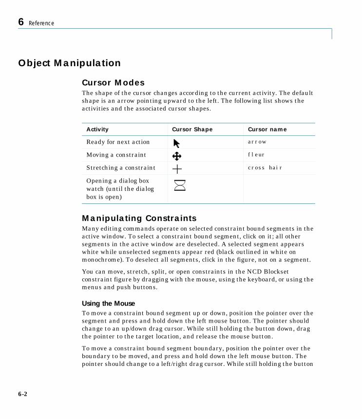
6 Reference

Object Manipulation

Cursor ModesThe shape of the cursor changes according to the current activity. The default shape is an arrow pointing upward to the left. The following list shows the activities and the associated cursor shapes.

Manipulating ConstraintsMany editing commands operate on selected constraint bound segments in the active window. To select a constraint bound segment, click on it; all other segments in the active window are deselected. A selected segment appears white while unselected segments appear red (black outlined in white on monochrome). To deselect all segments, click in the figure, not on a segment.

You can move, stretch, split, or open constraints in the NCD Blockset constraint figure by dragging with the mouse, using the keyboard, or using the menus and push buttons.

Using the MouseTo move a constraint bound segment up or down, position the pointer over the segment and press and hold down the left mouse button. The pointer should change to an up/down drag cursor. While still holding the button down, drag the pointer to the target location, and release the mouse button.

To move a constraint bound segment boundary, position the pointer over the boundary to be moved, and press and hold down the left mouse button. The pointer should change to a left/right drag cursor. While still holding the button

Activity Cursor Shape Cursor name

Ready for next action arrow

Moving a constraint fleur

Stretching a constraint cross hair

Opening a dialog box watch (until the dialog box is open)

6-2

Object Manipulation

down, drag the pointer to the target location, and release the mouse button. Notice that the segments on either side of the boundary maintain their slopes.

To stretch a constraint bound segment, position the pointer just on the inside edge of the segment to be stretched and press and hold down the mouse button. The pointer should change to a fleur. While still holding the button down, drag the pointer to the target location, and release the mouse button. Note that short constraints may have to be stretched before they can be moved.

To split a constraint bound segment at a particular position, position the pointer over the segment to be split at the location you want to split the constraint, hold down the shift key and press the left mouse button (extended SelectionType). The segment splits where the pointer is and the segment to the left of the pointer selected. If you continue to hold down the left mouse button after splitting the segment, the selected segment can be stretched as described above.

To open a constraint bound segment, hold down the control key and press the left mouse button (alternate Selection Type). Opening a constraint bound segment creates a Constraint Editor dialog box. From the Constraint Editor dialog box, the selected constraint bound segment can be weighted. The Constraint Editor allows you to specify exactly the selected segment’s position using the Position editor [x1 y1 x2 y2] field. Selecting a different constraint bound segment updates the Constraint Editor. If no constraints in the current constraint figure are selected, the Constraint Editor is destroyed.

Using the KeyboardKeypress shortcuts allow you to perform all constraint manipulations using the keyboard. To use keypress shortcuts, the pointer must be on the appropriate NCD constraint figure. The following table summarizes how constraint bounds can be moved using keypress shortcuts.

6-3

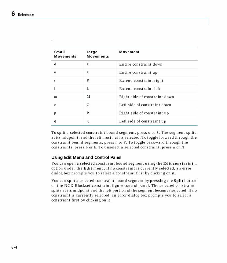
6 Reference

.

To split a selected constraint bound segment, press s or S. The segment splits at its midpoint, and the left most half is selected. To toggle forward through the constraint bound segments, press f or F. To toggle backward through the constraints, press b or B. To unselect a selected constraint, press n or N.

Using Edit Menu and Control PanelYou can open a selected constraint bound segment using the Edit constraint... option under the Edit menu. If no constraint is currently selected, an error dialog box prompts you to select a constraint first by clicking on it.

You can split a selected constraint bound segment by pressing the Split button on the NCD Blockset constraint figure control panel. The selected constraint splits at its midpoint and the left portion of the segment becomes selected. If no constraint is currently selected, an error dialog box prompts you to select a constraint first by clicking on it.

SmallMovements

LargeMovements

Movement

d D Entire constraint down

u U Entire constraint up

r R Extend constraint right

l L Extend constraint left

m M Right side of constraint down

z Z Left side of constraint down

p P Right side of constraint up

q Q Left side of constraint up

6-4

NCD Blockset Menus

NCD Blockset MenusThe NCD Blockset menus appear on your particular platform in the same way as SIMULINK menus.

Menu items followed by a right arrow lead to a submenu. Menu items followed by an ellipsis lead to a settings dialog box. Stand-alone menu items result in a direct action.

You can execute some menu items by using keyboard accelerators. You invoke NCD Blockset accelerators in the same way you do SIMULINK accelerators. Learning to use the accelerator keys can significantly improve the efficiency of your NCD Blockset sessions.

The following sections describe the NCD Blockset menus and the dialog boxes associated with menu items.

6-5

6 Reference

File MenuLoad Select a set of constraints and constraint data to load from disk.

Close Remove the NCD constraint figure from the screen.

Save Write a set of constraints and constraint data to a file.

Print Print the Constraint axes.

Load...

Load displays a dialog box with a list of existing files from which you can select the file you want to display. You can list the contents of a different directory by changing the path in the selection box. You can view more filenames by moving the scroll bar up or down. You can select a file by double-clicking on that filename or by typing the filename in the edit field and then clicking on the Open button. When you select a file, the new constraints are loaded into the workspace and displayed in all appropriate NCD Blockset figures.

6-6

File Menu

Save...

Save displays a dialog box for specifying the name of the file in which to save the constraints and other data used by the NCD Blockset. You can save the constraints to a currently existing file or enter a new name. You can also change the directory in which the constraints are saved (essentially, making a copy in another location).

6-7

6 Reference

Edit MenuUndo Undo the previous constraint bound edit.

Edit constraint... Edit the selected constraint bound segment.

Delete plots Delete all lines in the current NCD figure.

Edit constraint...

Edit constraint displays a dialog box for specifying the constraint bound segment weight and position. To open the Constraint Editor dialog box either control-click (Alternate Selection Type) on a constraint bound or select Edit constraint... from the Edit menu while a constraint is selected. The Constraint Editor dialog box appears as shown above.

Use the Position editor [x1 y1 x2 y2] editable text field to precisely place a constraint. You can also change the weighting associated with a constraint bound segment using the Constraint Editor dialog box. By default, all constraints possess weight equal to one. Any constraint with weight greater than zero is classified as an overachieving constraint. This means that the cost function of the optimization is such that even after the response has met the constraints, further improvement in the optimization cost function may be possible (i.e., the optimizer attempts to drive the response away from the constraint). A weight of zero implies a hard constraint. This means that once the constraints have been met, no further improvement in the cost function can be made. A more technical explanation of constraint weighting can be found in the Appendix.

6-8

Options Menu

Options MenuInitial response Plot initial response of system.

Reference input... Define reference signal.

Step response... Specify step response characteristics.

Time range... Choose range of axes

Y-Axis... Change Y-axis limits.

Refresh Redisplay all constraints for this output.

Reference input...

Reference input displays a dialog box for specifying a reference input for the constrained output. The reference input does not affect the SIMULINK system. It merely plots the lines specified by the time vector and input vector lines.

6-9

6 Reference

Step response...

Step response displays a dialog box for specifying step response characteristics. The dialog box operates on constraints between the step time and the final time. Changes to the constraint bound segments occur when the editable text field control callback executes. Entering a settling time without a percent settling value results in a default five percent settling. Entering a rise time without a percent rise value results in a default 90 percent rise.

Time range...

Time range displays a dialog box which allows you to change the X-axis limits and label of the current NCD Blockset constraint figure. The dialog box expects you to input a 1 × 2 matrix for X axis limits. You can enter any string for X-axis label. Note that the values entered here only affect the time axis limits in the

6-10

Options Menu

current NCD figure. To change the optimization start and stop times use the Simulation Parameters dialog box in your SIMULINK model.

Y-Axis...

Y-Axis displays a dialog box which allows you to change the Y-axis limits and label of the current NCD Blockset constraint figure. The dialog box expects you to input a 1-by- 2 matrix for Y-axis limits. You can enter any string for Y-axis label.

6-11

6 Reference

Optimization MenuStart Start optimization of tunable variables.

Stop Stop optimization if one is in progress.

Parameters... Edit optimization parameters.

Uncertainty... Edit uncertainty variables.

Parameters...

Parameters displays a dialog box for specifying the tunable variables and other optimization parameters (such as lower and upper bounds on the tunable variables and discretization interval) to be used in the current optimization. You can disable the display from the optimization routine (to the MATLAB command window) by checking off the Display optimization information check box.

By default, the optimization routine does not stop as soon as all the constraints are met, it tries to overachieve. If you wish to stop as soon as the constraints are met, then enable the Stop optimization as soon as the constraints are achieved check box.

6-12

Optimization Menu

You can specify the optimization routine to use a separate routine (see gradfun.m) for computing the gradients by enabling the Compute gradients with better accuracy (slower) check box.

Uncertainty...

Uncertainty displays a dialog box for specifying the uncertain variables and other uncertainty information (such as lower and upper bounds on the uncertain variables and number of Monte Carlo simulations to run) to be used in the current optimization.

6-13

6 Reference

Style MenuGrid Toggle grid display.

Snap Toggle 22.5 degree snap.

Hot-key help... Show help on menu accelerators and keypress shortcuts.

6-14

NCD Blockset Control Panel

NCD Blockset Control PanelThe NCD Blockset control panel is available at the bottom of the NCD Blockset constraint figure.

Port displays the port number of the constraint signal in the SIMULINK model corresponding to this figure. You can enter the port number of any other NCD blocks in the model to switch the figure window from one constrained signal to another. The number you enter in this editable text field should correspond to the port number of an NCD block, which is in fact a masked outport block.

Split splits a selected constraint bound segment at its midpoint leaving the left half of the segment as the selected segment. If no constraint bound segments are currently selected, an error dialog is displayed.

Start begins the optimization of tunable variables.

Stop halts the optimization when pressed while the optimization is in progress.

Help creates a general NCD Blockset Help dialog box.

Close removes the NCD Blockset constraint figure from the screen. If you have made changes to the constraints or other NCD Blockset variables, a dialog box asks you if you want to save the NCD Blockset constraints and data to a file.

6-15

6 Reference

6-16

A

Appendix

A Appendix

This appendix to the NCD Blockset discusses the following areas:

• Optimization Details

• Representation of Time Domain Constraints

• NCD Global Variable: ncdStruct

• LQR Design for Inverted Pendulum

A-2

Optimization Details

Optimization Details This section discusses the details of the optimization invoked when you press the Start button or select the Start menu item from the Optimization menu. Because the NCD Blockset automates the entire optimization process, familiarity with these details is not required and this section may be considered optional.

Problem Formulation DetailsThe constraint bounds displayed in the NCD Blockset constraint window are for visualization purposes only. Two matrices, ncdStruct.CnstrLB andncdStruct.CnstrUB, contain all the constraint information. See the next section for more information about how ncdStruct.CnstrLB andncdStruct.CnstrUB store constraint data and for a summary of other fields of the global variable ncdStruct defined by the NCD Blockset. For now, it is enough to know that each constraint bound matrix consists of groups of weighted line segment data for each output constrained.

When the optimization is started, the NCD Blockset invokes the routine nlinopt. Generation of the optimization problem involves three steps:

1 Processing uncertainty data

2 Expanding the constraint matrices ncdStruct.CnstrLB and ncd-Struct.CnstrUB.

3 Invoking the constrained optimization routine constr

The NCD Blockset routine montevar processes uncertainty data input to the Uncertain Variables dialog box. It generates Monte Carlo plant data and performs certain error checks. The routine produces the Monte Carlo plants assuming a uniformly distributed probability density between the lower and upper bounds entered into the Uncertain Variables dialog box.

The NCD Blockset routine convertm expands the constraint matrices, ncdStruct.CnstrLB and ncdStruct.CnstrUB, using the discretization interval Td = ncdStruct.Tdelta. Generally speaking, constraints are generated at an interval of Td, per constraint segment per constrained signal.

A-3

A Appendix

After more error checking, nlinopt vectorizes the tunable variables and invokes the constrained optimization routine constr. Specifically, if you input V1 V2... as tunable variables into the Optimization Parameters dialog box, the NCD Blockset passes the vector x = [V1(:); V2(:); ... gamma] to constr. By calling constr with a special option flag, it expects gamma to contain the value of the cost function. The NCD Blockset problem formulation defines the cost function as the (weighted) maximum constraint violation. The constr routine perturbs each tunable variable in turn and evaluates the resulting cost function and constraint equations. After determining a gradient (search direction) from this information, constr performs a line search along the gradient in an attempt to simultaneously minimize the cost while satisfying constraint equations.

The NCD Blockset routine costfun returns the cost function and constraints. As mentioned above, costfun calculates the cost function

CostFunction = x(length(x)); % i.e. gamma

which corresponds to the (weighted) maximum constraint violation. The routine then initializes the constraint vector to the empty matrix and recovers (defines) the tunable variables from the vector x described above. Next, it initiates a for loop according to the number of plants constrained, Npc. Specifically, Npc is the number of Monte Carlo simulations to be constrained plus the nominal, upper bound, and lower bound plant if they are constrained.

Within each for loop, costfun assigns the uncertain plant variables (as defined by the routine montevar) and calls for a simulation. It next linearly interpolates the simulation output to the time basis Tstart:Td:Tstop using the table1 command. If necessary, it updates the plots of any open NCD constraint figures. Finally, it augments the constraint vector.

To describe the constraint vector in detail, we define

Yout a length(Tstart:Td:Tfinal) by p matrix corre-sponding to the linearly interpolated simulation output (i.e., the SIMULINK system has p NCD-masked Outport blocks)

A-4


Then convertm defines Mu and Ml, which have three columns described by

Given this, each pass through the for loop augments the constraint vector, ConstraintError, as

ConstraintError = [ConstraintError; ...Yout(Mu(:,1)) – Mu(:,2) – Mu(:,3)*CostFunction; ...

Ml(:,2) – Yout(Ml(:,1)) – Ml(:,3)*CostFunction];

which implies that the system response should be less than upper bound constraints and greater than lower bound constraints.

Ml [AbsoluteYoutIndex Bound Weight]

Mu [AbsoluteYoutIndex Bound Weight]

A-5

A Appendix

The following pseudocode summarizes the optimization.

% Begin nlinopt% Process uncertain variable information (montevar)% Expand constraint matrices (convertm)% Initialize arguments for constr.m

% Begin constrwhile ~(termination_criterion_met),

for 1:Ntp, % Number of tunable parameters% Begin costfun% Calculate cost function (CostFunction)% Set tunable variablesfor 1:Npc, % Number of plants constrained

% Assign plant uncertain variables% Call for simulation% Convert simulation time index% Draw necessary plots% Calculate constraints% Append constraints into vector % i.e ConstraintError

end % for Ntp% End costfun

% Tweak tunable variables in turnend % for Ntp% Calculate gradient information% Define search direction% Perform line search% Determine termination_criterion_met

end% End constr% End nlinopt

Notice that the number of simulations conducted at each iteration is given by

Ns = Ntp*Npc + O(1)

where Ntp is the total number of elements in the tunable parameters and Npc is the number of plants constrained as defined above. The extra term O(1) arises due to the line search, which is discussed in the next section. The term O(1) does not depend on either Ntp or Npc and is typically one. To decrease your

A-6


optimization time, you should constrain as few plants and tune as few variables as possible. For example, when you optimize with uncertainty, try constraining only the upper and lower bound plant (i.e., do not constrain the nominal plant or any Monte Carlo generated plants). Once the optimization has completed, inspect the nominal plant response and a number of Monte Carlo plant responses by checking the appropriate boxes in the Uncertain Variables dialog box and selecting Initial response from the Options menu.

Each constrained output generates approximately2*Npc*floor((Tstop–Tstart)/Td) constraints, where Npc equals the number of plants constrained, Tstop is the simulation stop time, Tstart is the simulation start time, and Td is the discretization interval. More specifically, each constraint bound segment defined between time T1 and T2 (T2>T1) generates exactly floor((T2–T1)/Td) constraints for each plant constrained. Since the optimization routine generates a square matrix of the same size as the number of constraints, care must be taken not to generate too many constraints for risk of encountering memory problems. Choosing a discretization interval of between 1 and 2 percent of the total simulation time should keep you safe from Out of memory errors while at the same time generating enough constraints to satisfactorily approximate the continuous time constraint bounds of the constraint figures.

Optimization Algorithmic DetailsAs mentioned in Chapter 2, the NCD Blockset transforms the constraints and simulated system output into an optimization problem of the form

where the boldface characters denote vectors. This type of optimization problem is solved in the Optimization Toolbox routine constr. In reference to the last section,

γ gammag(x)- w γ ConstraintErrorx x

min γx γ, s.t.

g x⟨ ⟩ wγ– 0≤xl x xu≤ ≤

A-7

A Appendix

The Sequential Quadratic Programming (SQP) method used by constr solves a Quadratic Programming (QP) problem at each iteration and updates an estimate of the Hessian of the Lagrangian. The line search is performed using a merit function. The routine uses an active set strategy for solving the QP subproblem.

The implementation of the SQP subproblem attempts to satisfy the Kuhn-Tucker equations, which are necessary conditions for optimality of a constrained optimization problem. The principal idea of the SQP algorithm forms a QP problem at each iteration based on the quadratic approximation of the Lagrangian function.

The QP solution procedure involves two phases: the first phase involves the calculation of a feasible point (if one exists); the second phase involves the generation of an iterative sequence of feasible points, which converge to the solution. In this method, an active set is maintained of the active constraints at the solution point. Virtually all QP algorithms are active set methods. This point is emphasized because many different methods exist, which are very similar in structure but which are described in widely different terms.

The routine constr further exploits the special structure of the constrained problem. For example, it can be shown from the Kuhn-Tucker equations that the approximation to the Hessian of the Lagrangian, should have zeros in the rows and columns associated with the variable γ. However, this results in only a positive semi-definite Hessian which requires a more elaborate (slow) QP solution technique. Instead the algorithm initializes the Hessian matrix with ones along its diagonal except for the element associated with γ, which is initialized to a small positive number (e.g., 1e-10). Throughout the optimization, the code maintains zeros in all rows and columns of the Hessian associated with γ except the diagonal element, which is maintained at the small number. This allows the code to use a fast converging positive definite QP method while at the same time exploiting the problem’s special structure.

The routine constr relates the status of the QP algorithm in the last column of the display output (the column labeled Procedures). Generally no display appears in the column meaning the Hessian is positive definite. For nonpositive definite Hessians, two successive modifications can be performed to make the Hessian positive definite. If the first modification succeeds, the message mod Hess appears in the Procedures column. The second modification always results in a positive definite Hessian and displays mod Hess(2) in the Procedures column. Often such messages imply that the optimization is far

A-8


from a solution or that the problem is particularly sensitive to variations in some of the tunable parameters.

A nonlinearly constrained problem can often be solved in fewer iterations using SQP than an unconstrained problem. One of the reasons for this is that, due to the limits on the feasible area, the optimizer can make well informed decisions regarding directions of search and step length. This characteristic of the nonlinearly constrained problem is advantageous to the NCD problem formulated since calculation of the cost function is computationally time consuming (it requires simulation of the system). Time saved due to fewer iterations more than compensates for the additional overhead associated with the constrained formulation.

For more information on the algorithms discussed in this section, see the Optimization Toolbox User’s Guide.

A-9

A Appendix

Representation of Time Domain ConstraintsThis section discusses the constraint bounds displayed in the NCD Blockset constraint window, which are for visualization purposes only. All constraint information is contained in two matrices, ncdStruct.CnstrLB andncdStruct.CnstrUB, which are fields of the global structure variablencdStruct. Each constraint bound consists of groups of line segment data for each output constrained.

The matrix ncdStruct.CnstrLB (ncdStruct.CnstrUB) has dimension 4 × 2L where L is the total number of line segments in all lower (upper) bounds. The first row of ncdStruct.CnstrLB and ncdStruct.CnstrUB contains the outport number for the constraint. All constraint bound segments for the same outport are grouped together. The second row contains the time axis values of the segment while the third row contains the response axis values. The time axis values for each output increase monotonically from optimization start time to optimization stop time. The time value end of one segment equals the time value beginning of the next segment. The fourth row of ncdStruct.CnstrLB (ncdStruct.CnstrUB) contains information about the segment’s weighting.

As an example, consider the lower bound constraint matrix,

The matrix’s first row shows that two outputs are constrained. The first output is constrained by three line segments and the second by one line segment. Constraints on the second output are defined by the line segment from the (time, response) point (0,-0.1) to the point (100,-0.1). Constraints on the first output are defined by the line segments from (0,0) to (10,0), from (10,0.9) to (30,0.9), and from (30,0.99) to (100,0.99). We expect a simulation start time of zero and stop time of 100. The fourth row shows that all line segments are weighted equally, with weight of one (the even columns of the fourth row are reserved for future use).

ncdStruct.CnstrLB

1 1 1 1 1 1 2 20 10 10 30 30 100 0 1000 0 0.9 0.9 0.99 0.99 0.1– 0.1–

1 0 1 0 1 0 1 0

=

A-10

NCD Global Variable ncdStruct

NCD Global Variable ncdStructThis section discusses the fields in the global variable ncdStruct that is created in your workspace when using the NCD Blockset. Clearing these variables or changing them in unexpected ways causes the NCD Blockset to generate errors from which you may not be able to recover.

These variables are associated with the NCD optimization problem:

ncdStruct.TvarStr Single row string containing the names of the tunable variables. This string is changed via the Tunable Variables edit field on the Tunable Variables dialog box.

ncdStruct.TvlbStr Single row string which, when evaluated, defines a lower bound on the tunable variables. This string is changed via the Lower bounds edit field on the Tunable Variables dialog box.

ncdStruct.TvubStr Single row string which, when evaluated, defines an upper bound on the tunable variables. This string is changed via the Upper bounds edit field on the Tunable Variables dialog box

ncdStruct.Tdelta Scalar defining the discretization interval. This scalar is changed via the Discretization interval edit field on the Tunable Variables dialog box.

ncdStruct.CostFlag Boolean equal to 1 if optimization should con-tinue even after achieving the constraints. This Boolean is changed via the Stop optimization as soon as the constraints are achieved check box on the Tunable Variables dialog box.

ncdStruct.GradFlag Boolean equal to 1, if the optimization routine is specified to use an accurate method for gradi-ents. This Boolean is changed via the Compute gradients with better accuracy (slower) check box on the Tunable Variables dialog box.

A-11

A Appendix

Variables associated with plant uncertainty:

ncdStruct.OptmOptns Vector sets various optimization options as defined in the Optimization Toolbox User’s Guide. Some elements of this vector are changed via the Display check box and Terminate for x and Terminate for g edit fields on the Tunable Parameters dialog box.

ncdStruct.UvarStr Single row string containing the names of the uncertain variables. This string is changed via the Uncertain Variables edit field on the Uncer-tain Variables dialog box.

ncdStruct.UvlbStr Single row string which, when evaluated, defines a lower bound on the uncertain variables. This string is changed via the Lower bound edit field on the Uncertain Variables dialog box.

ncdStruct.UvubStr Single row string which, when evaluated, defines a lower bound on the uncertain variables. This string is changed via the Upper bound edit field on the Uncertain Variables dialog box.

ncdStruct.NumMC Scalar number of Monte Carlo plants to be gener-ated.

ncdStruct.PlntON 1-by-4 vector of Booleans relating whether nom-inal plant, lower bound uncertain plant, upper bound uncertain plant, and Monte Carlo plants are to be included in the optimization.

A-12

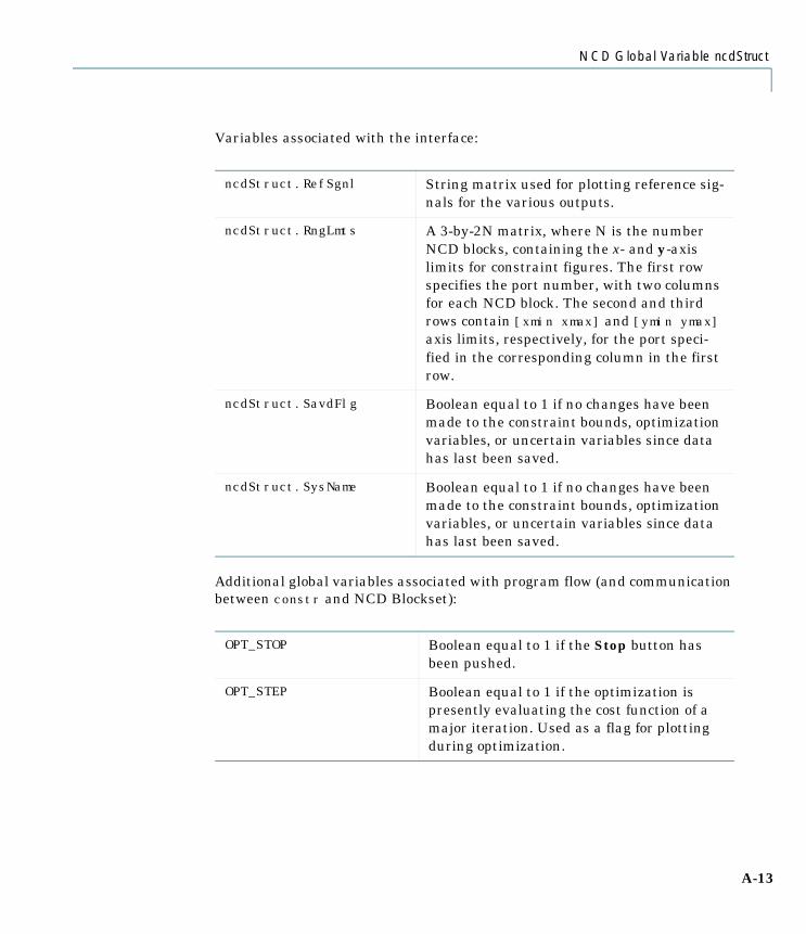
NCD Global Variable ncdStruct

Variables associated with the interface:

Additional global variables associated with program flow (and communication between constr and NCD Blockset):

ncdStruct.RefSgnl String matrix used for plotting reference sig-nals for the various outputs.

ncdStruct.RngLmts A 3-by-2N matrix, where N is the number NCD blocks, containing the x- and y-axis limits for constraint figures. The first row specifies the port number, with two columns for each NCD block. The second and third rows contain [xmin xmax] and [ymin ymax] axis limits, respectively, for the port speci-fied in the corresponding column in the first row.

ncdStruct.SavdFlg Boolean equal to 1 if no changes have been made to the constraint bounds, optimization variables, or uncertain variables since data has last been saved.

ncdStruct.SysName Boolean equal to 1 if no changes have been made to the constraint bounds, optimization variables, or uncertain variables since data has last been saved.

OPT_STOP Boolean equal to 1 if the Stop button has been pushed.

OPT_STEP Boolean equal to 1 if the optimization is presently evaluating the cost function of a major iteration. Used as a flag for plotting during optimization.

A-13

A Appendix

LQR Design for Inverted PendulumChapters 2 and 4 contain examples of an inverted pendulum system. Both examples assume that an initial stabilizing LQR controller exists. This section details how that controller is generated.

Recall that, ignoring motor dynamics, the nonlinear equations of motion for the inverted pendulum system are

where

f Force applied to the cart by motor in Newtons

Position of cart in meters

y Angle of pendulum from vertical in radians

Θ Mass of cart (0.455kg)

M Mass of pendulum (0.21kg)

l Distance to center of mass of pendulum (i.e., one half its length of 0.61m

g Acceleration of gravity (9.8m/s^2)

A-14

LQR Design for Inverted Pendulum

These equations may be linearized about the operating point y = 0 andΘ = 0 to yield the linear system

Using the MATLAB command

Klqr = lqr(A,b,diag([0.25 0 4 0],0.003)

produces the stabilizing gain

Klqr = [–28.8675 –28.5632 –145.0014 –14.8601]

which is the initial stabilizing gain used in Chapters 2 and 4.

A-15

A Appendix

A-16

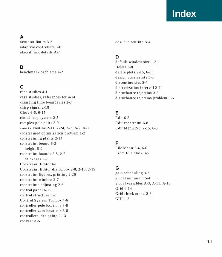
Index

Aactuator limits 3-3adaptive controllers 3-6algorithmic details A-7

Bbenchmark problems 4-2

Ccase studies 4-1case studies, references for 4-14changing time boundaries 2-8chirp signal 2-18Close 6-6, 6-15closed loop system 2-5complex pole pairs 3-9constr routine 2-11, 2-24, A-3, A-7, A-8constrained optimization problem 1-2constraining plants 2-14constraint bound 6-2

height 5-9constraint bounds 2-5, 2-7

thickness 2-7Constraint Editor 6-8Constraint Editor dialog box 2-8, 2-18, 2-19constraint figures, printing 2-26constraint window 2-7constraints adjusting 2-6control panel 6-15control structure 5-2Control System Toolbox 4-6controller pole locations 3-8controller zero locations 3-8controllers, designing 2-13convert A-5

costfun routine A-4

Ddefault window size 1-3Delete 6-8delete plots 2-15, 6-8design constraints 3-3discontinuities 5-4discretization interval 2-24disturbance rejection 3-5disturbance rejection problem 3-5

EEdit 6-8Edit constraint 6-8Edit Menu 2-3, 2-15, 6-8

FFile Menu 2-4, 6-6From File block 3-5

Ggain scheduling 3-7global minimum 5-4global variables A-3, A-11, A-13Grid 6-14Grid check menu 2-8GUI 1-2

I-1

Index

I-2

HHelp 6-15Help button 6-10Hot-key help 6-14

Iill posed message 5-5infeasible message 5-5initial conditions 5-3Initial response 2-13, 2-15, 6-9installation instructions 1-3integrated signals, minimization of 3-3inverted pendulum 2-16, 4-12, A-14inverted pendulum example 4-12

KKalman state estimator 4-6Kuhn-Tucker equations A-8

Llevels of use 4-3, 4-4, 4-6, 4-7, 4-10, 4-11, 4-12,

4-13, 4-14Load 6-6local minimum 5-4lqgdemos 4-6LQR 2-16

design for inverted pendulum A-2, A-14with feedforward controller 4-6

LV100 gas turbine engine 4-9

Mmenus

Edit 6-8

File 6-6Options 6-9

MIMO 3-6MIMO PI controller 4-9minimizing integrated signals 3-3models

analyzing 2-24, 2-25, A-3Monte Carlo A-7

option 2-15simulations 1-2

moving constraints 6-2multimode control 3-6multimode controllers 3-6

NNCD block 1-2, 2-6NCD global variables A-2, A-11NCD menu bar 2-6NCD Toolbox Control Panel 6-15NCD_LB A-3, A-10NCD_UB A-3, A-10ncdblock 2-3ncddemo1 4-2, 4-3ncddemo2 4-2, 4-6ncddemo3 4-2, 4-9ncddemo4 4-2, 4-12ncdStruct.CnstrLB 2-25ncdStruct.CnstrUB 2-25ncdStruct.CostFlag 2-25ncdStruct.GradFlag 2-25ncdStruct.RngLmts 2-25ncdStruct.SysName 2-25ncdStruct.Tdelta 2-25ncdStruct.TvarStr 2-25nlinopt routine A-3

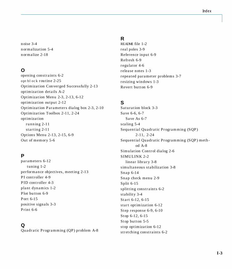
Index

noise 3-4normalization 5-4normalize 2-18

Oopening constraints 6-2optblock routine 2-25Optimization Converged Successfully 2-13optimization details A-2Optimization Menu 2-3, 2-13, 6-12optimization output 2-12Optimization Parameters dialog box 2-3, 2-10Optimization Toolbox 2-11, 2-24optimization

running 2-11starting 2-11

Options Menu 2-13, 2-15, 6-9Out of memory 5-6

Pparameters 6-12

tuning 1-2performance objectives, meeting 2-13PI controller 4-9PID controller 4-3plant dynamics 1-2Plot button 6-9Port 6-15positive signals 3-3Print 6-6

QQuadratic Programming (QP) problem A-8

RREADME file 1-2real poles 3-9Reference input 6-9Refresh 6-9regulator 4-6release notes 1-3repeated parameter problems 3-7resizing windows 1-3Revert button 6-9

SSaturation block 3-3Save 6-6, 6-7

Save As 6-7scaling 5-4Sequential Quadratic Programming (SQP)

2-11, 2-24Sequential Quadratic Programming (SQP) meth-

od A-8Simulation Control dialog 2-6SIMULINK 2-2

linear library 3-8simultaneous stabilization 3-8Snap 6-14Snap check menu 2-9Split 6-15splitting constraints 6-2stability 3-4Start 6-12, 6-15start optimization 6-12Step response 6-9, 6-10Stop 6-12, 6-15Stop button 5-5stop optimization 6-12stretching constraints 6-2

I-3

Index

I-4

strong stabilization requirements 3-9Style Menu 2-3, 2-8, 2-9, 6-14system identification 2-5, 3-5

closed loop 2-16system requirements 1-3

Ttime domain constraints A-2, A-10Time range 6-9, 6-10tracking 3-5, 4-3, 4-6, 4-10, 4-12troubleshooting 5-1Tunable Parameters dialog box 2-23typical problems 5-2typographical conventions 1-3

UUncertain Variables dialog box 2-3, 2-13Uncertainty 6-12, 6-13uncertainty 1-2

adding 2-13Undo 6-8undo previous edit 6-8Using SIMULINK manual 2-2NCD Toolbox User’s Guide 2-5

YY-axis 6-9, 6-11

Range dialog box 2-19

ZZiegler-Nichols 4-4

Modeling Simulation Implementation - cvut.czradio.feld.cvut.cz/matlab/pdf_doc/ncd/ncd_blks.pdf · 2...

Documents

Transcript of Modeling Simulation Implementation - cvut.czradio.feld.cvut.cz/matlab/pdf_doc/ncd/ncd_blks.pdf · 2...