Modeling Raindrop Size - ww2.amstat.orgww2.amstat.org/publications/jse/v23n1/johnson.pdf ·...
26
Journal of Statistics Education, Volume 23, Number 1 (2015) 1 Modeling Raindrop Size Roger W. Johnson Donna V. Kliche Paul L. Smith South Dakota School of Mines & Technology Journal of Statistics Education Volume 23, Number 1 (2015), www.amstat.org/publications/jse/v23n1/johnson.pdf Copyright © 2015 by Roger W. Johnson, Donna V. Kliche and Paul L. Smith, all rights reserved. This text may be freely shared among individuals, but it may not be republished in any medium without express written consent from the authors and advance notification of the editor. Key Words: Distribution; Exploratory Data Analysis; Parameter Estimation; Maximum Likelihood; Disdrometer; Beta Density; Exponential Density; Gamma Density; Lognormal Density; Weibull Density. Abstract Being able to characterize the size of raindrops is useful in a number of fields including meteorology, hydrology, agriculture and telecommunications. Associated with this article are data sets containing surface (i.e. ground-level) measurements of raindrop size from two different instruments and two different geographical locations. Students may begin to develop some sense of the character of raindrop size distributions through some basic exploratory data analysis of these data sets. Teachers of mathematical statistics students will find an example useful for discussing the beta, gamma, lognormal and Weibull probability density models, as well as fitting these by maximum likelihood and assessing the quality of fit. R software is provided by the authors to assist students in these investigations. 1. Introduction The distributions of raindrop size are of interest to meteorologists who use them as an input into numerical weather prediction models, to telecommunications engineers who are concerned with potential signal loss and to hydrologists who are interested in the total volume of water falling (Brawn and Upton 2007). Additionally, raindrop size distribution is related to soil erosion, visibility and radar reflectivity (Brawn and Upton 2008). Drop size distribution varies from storm to storm, over the duration of a storm, and according to location within the storm. In particular, the atmospheric drop size distribution is different from that recorded at the surface of
Transcript of Modeling Raindrop Size - ww2.amstat.orgww2.amstat.org/publications/jse/v23n1/johnson.pdf ·...

Journal of Statistics Education, Volume 23, Number 1 (2015)
1
Modeling Raindrop Size
Roger W. Johnson
Donna V. Kliche
Paul L. Smith
South Dakota School of Mines & Technology
Journal of Statistics Education Volume 23, Number 1 (2015),
www.amstat.org/publications/jse/v23n1/johnson.pdf
Copyright © 2015 by Roger W. Johnson, Donna V. Kliche and Paul L. Smith, all rights reserved.
This text may be freely shared among individuals, but it may not be republished in any medium
without express written consent from the authors and advance notification of the editor.
Key Words: Distribution; Exploratory Data Analysis; Parameter Estimation; Maximum
Likelihood; Disdrometer; Beta Density; Exponential Density; Gamma Density; Lognormal
Density; Weibull Density.
Abstract
Being able to characterize the size of raindrops is useful in a number of fields including
meteorology, hydrology, agriculture and telecommunications. Associated with this article are
data sets containing surface (i.e. ground-level) measurements of raindrop size from two different
instruments and two different geographical locations. Students may begin to develop some sense
of the character of raindrop size distributions through some basic exploratory data analysis of
these data sets. Teachers of mathematical statistics students will find an example useful for
discussing the beta, gamma, lognormal and Weibull probability density models, as well as fitting
these by maximum likelihood and assessing the quality of fit. R software is provided by the
authors to assist students in these investigations.
1. Introduction
The distributions of raindrop size are of interest to meteorologists who use them as an input into
numerical weather prediction models, to telecommunications engineers who are concerned with
potential signal loss and to hydrologists who are interested in the total volume of water falling
(Brawn and Upton 2007). Additionally, raindrop size distribution is related to soil erosion,
visibility and radar reflectivity (Brawn and Upton 2008). Drop size distribution varies from
storm to storm, over the duration of a storm, and according to location within the storm. In
particular, the atmospheric drop size distribution is different from that recorded at the surface of

Journal of Statistics Education, Volume 23, Number 1 (2015)
2
the Earth; drop growth takes place within the clouds, the larger drops fall with greater velocity,
and the largest drops may tend to break up as they fall.
It should be mentioned that while a droplet clinging to a surface (e.g. a faucet) is teardrop-
shaped, raindrops falling through the atmosphere are not so shaped (see, for example,
http://en.wikipedia.org/wiki/Drop_(liquid)). Smaller drops, less than 1 mm in diameter, say, tend
to be nearly spherical in shape. Somewhat larger drops are flatter on the bottom due to the
pressure of the air – so drops in this case may be thought of as being in the shape of small
hamburger buns. For us, raindrop size will refer to raindrop diameter; for the larger drops we
mean the diameter of a volume-equivalent sphere.
The data sets associated with this article contain surface measurements from two different types
of disdrometers, as devices that measure raindrop sizes are called. The Joss-Waldvogel (JW)
disdrometer converts raindrop mechanical impacts into electrical signals that can be used to
estimate drop size. The JW disdrometer is able to measure drop diameters in the range from
about 0.3 mm to about 5.5 mm and does so with an accuracy of within 5% error (Tokay, Bashor
and Wolff 2005, p. 514). The Parsivel disdrometer, Parsivel short for PARticle SIze and
VELocity, estimates both raindrop diameter and fall velocity. Here, the drop size is estimated
through the change in light intensity that occurs as drops fall through an optical beam. The
velocity is estimated by using the time it takes to travel through the beam. The Parsivel
disdrometer also generally fails to see drops with diameters below 0.3 mm but can potentially
record drop sizes quite a bit larger than that of the JW disdrometer (Kliche 2007). The Parsivel
disdrometer is generally considered to be somewhat less accurate in determining drop diameters
than the JW disdrometer (c.f. Löffler-Mang and Joss 2000).
Pictures of these two disdrometers may be found, for example, on the Karlsruhe Institute of
Technology pages. See https://www.imk-tro.kit.edu/english/1289.php and https://www.imk-
tro.kit.edu/english/1291.php.
Teachers may help students achieve the following learning objectives, among others, with the
help of the discussion below and the accompanying disdrometer data along with the R code (R
Development Core Team 2009, version 3.0.3, 64-bit) provided:
All students should be able to determine, through exploratory data analysis, general
features of raindrop diameter distributions. In particular, through their data analysis,
students should be able to answer the following questions:
o How large and how variable are raindrops in size during a storm?
o What is the storm to storm variability?
o How can we generally characterize the distribution shape of raindrop sizes?
o What is the probability of seeing a raindrop diameter between two specified
values?
Students in, or who have had, a course in Mathematical Statistics should:
o Recognize beta, gamma, lognormal and Weibull probability densities as potential
parametric models for raindrop size
o Understand how maximum likelihood estimation is performed with truncated and
binned data. In particular, that the likelihood is necessarily multinomial with (bin)

Journal of Statistics Education, Volume 23, Number 1 (2015)
3
probabilities which are integrals of the scaled (so as to integrate to one) density
model
o Understand how to assess the performance of a particular collection of density
models by using Pearson’s goodness of fit statistic
2. The Data
There are two data sets associated with this article. One data set contains surface observations
from a JW disdrometer in one-minute intervals in the Kwajalein Atoll in the Marshall Islands on
October 17, 2010; the first minute of observations begins at 00:00 UTC and the last minute of
observations begins at 23:59 UTC. That is, the Kwajalein data set contains observations each
minute over an entire day. The Kwajalein site lies at 8 deg north latitude in the mid Pacific, and
the rainfall is tropical in nature. The Kwajalein data set can be found at:
http://www.amstat.org/publications/jse/v23n1/johnson/JW.txt
The second data set contains surface observations from a Parsivel disdrometer in one-minute
intervals in Huntsville, AL on November 8, 2009; the first minute of observations begins at
09:44 UTC and the last minute of observations begins at 19:55 UTC. The Parsivel data from
Huntsville in northern Alabama generally represent subtropical continental rainfall. For the
Huntsville data there are quite a number of intervals where no observations have been recorded.
We opt not to list all of these here, but 463 one-minute collection periods out of the 612 minute
intervals from 09:44 through 19:55 may be found in the data set. The intervals with no
observations may correspond to periods of no rain or intermittent rain. The Huntsville data set
and can be found at: http://www.amstat.org/publications/jse/v23n1/johnson/Parsivel.txt.
The documentation file for both the Kwajalein and Parsivel data set can be found at:
http://www.amstat.org/publications/jse/v23n1/johnson/Raindrop_size_documentation.txt.
For both data sets we only see drop sizes within a restricted range of values – a “truncated-data”
problem. For the JW disdrometer, drop sizes between 0.313 mm and 5.600 mm are observed; for
the Parsivel disdrometer, drop sizes between 0.250 mm and 7.000 mm are observed. Since large
drop sizes are rare, most of the missing drops that fail to be seen are small drops. Furthermore,
both of these disdrometers only record counts of drops within specified bins – a “binned-data”
problem, instead of the actual drop sizes. In particular, we only see the counts of drops within
contiguous bins. A listing of these bins occurs in Table 1. For the Kwajalein data, drops are seen
in all of the bins displayed in the left-hand column of Table 1 (and none outside this range).
Likewise, for the Huntsville data, drops are seen in all of the bins displayed in the right-hand
column of Table 1 (and, again, none outside this range).

Journal of Statistics Education, Volume 23, Number 1 (2015)
4
Table 1. Disdrometer Bins for which we have Non-Zero Count Observations
Joss-Waldvogel Bins (mm)
Kwajalein Atoll Data
Parsivel Bins (mm)
Huntsville Data
[0.313, 0.405) [0.250, 0.375)
[0.405, 0.505) [0.375, 0.500)
[0.505, 0.596) [0.500, 0.625)
[0.596, 0.715) [0.625, 0.750)
[0.715, 0.827) [0.750, 0.875)
[0.827, 1.000) [0.875, 1.000)
[1.000, 1.233) [1.000, 1.125)
[1.233, 1.430) [1.125, 1.250)
[1.430, 1.583) [1.250, 1.500)
[1.583, 1.750) [1.500, 1.750)
[1.750, 2.079) [1.750, 2.000)
[2.079, 2.443) [2.000, 2.250)
[2.443, 2.730) [2.250, 2.500)
[2.730, 3.014) [2.500, 3.000)
[3.014, 3.388) [3.000, 3.500)
[3.388, 3.707) [3.500, 4.000)
[3.707, 4.130) [4.000, 4.500)
[4.130, 4.576) [4.500, 5.000)
[4.576, 5.145) [5.000, 6.000)
[5.145, 5.600) [6.000, 7.000)
To briefly summarize, both data sets – JW.txt and Parsivel.txt, contain records of the form
hour minute 1n 2n 20n
where the values 1n , 2n , , 20n are counts of observations in the bins given in Table 1 during a
one-minute period beginning at the specified hour and minute.
3. Exploratory Data Analysis
It is important to note that the two data sets only contain measurements over (a portion of) a day.
The raindrop size data are certainly not representative of what occurs over an annual or even a
seasonal time period. Therefore, any conclusions that are made are perhaps best qualified as
“with respect to the atmospheric conditions present” when the data were collected.
To explore the variability in raindrop size students may look both at individual minutes of
raindrop counts or a set of consecutive minutes of raindrop counts in each of the two data sets
provided. By opening the file JW.txt, for example, and, if necessary, adjusting the font size to see

Journal of Statistics Education, Volume 23, Number 1 (2015)
5
all 22 columns, we see a half-dozen or more storms (depending on how you decide to group
these) upon scrolling down the file (with intervening rows of all zeroes or mostly zeroes in the
last 20 columns). Figure 1, for example, shows a histogram of the rainfall collected during the
storms from 04:28 through 05:47.
Figure 1. Kwajelein JW Disdrometer Data 04:28– 05:47
This histogram may be produced by running the R script ML Rain.R
(http://www.amstat.org/publications/jse/v23n1/johnson/ML_Rain_16_Nov_2014.R) after editing
the code (the editing to be done is clearly marked at the beginning of the file) as follows:
data.read <- 2 # use 1 for the Parsivel data, 2 for the JW data
shour <- 4 # (starting) hour of first row of data to be included
sminute <- 28 # (starting) minute of first row of data to be included
ehour <- 5 # (ending) hour of last row of data to be included
eminute <- 47 # (ending) minute of last row of data to be included
(There are actually two histograms produced by running this R script, one with fitted curves
superimposed and one without. We defer discussion of the fitted curves to Sections 5 and 6.)

Journal of Statistics Education, Volume 23, Number 1 (2015)
6
The R script creates a variable midpts obtained by replacing the bin counts by like numbers of
numeric values at midpoints of the bin intervals. Using the variable midpts allows for
approximate calculation of numeric summaries. For the storm from 04:28 through 05:47, for
example, in which 52,318 drops were recorded, we find a mean drop size of about 1.6 mm, and a
standard deviation of about 0.47 mm, with quartiles of about 1.3 mm, 1.5 mm and 1.9 mm. The
commands summary(midpts) and sd(midpts) may be used in the R console window to
obtain these values.
We encourage instructors to have their students compare drop size numerically and graphically
across storms using the JW data in JW.txt. The Helpful Hint below indicates how boxplots may
be produced to compare two or more storms if graphical summaries other than histograms are
desired. Because of a lack of clear demarcation of storm events in the Huntsville data (in the
Parsivel.txt file) analysis of storm to storm variation is probably best restricted to the Kwajalein
data (the JW.txt file).
Helpful Hint: To produce side-by-side boxplots, after the first run of the code
(either data set, any time range) save the bin midpoints by executing the following
in the R console window:
midpts1 <- midpts
After the second run of the code (again, either data set, any time range) another
set of midpoints, midpts, is generated. Save these midpoints as well with
midpts2 <- midpts
Likewise save the midpoints for any subsequent runs and execute
boxplot(midpts1,midpts2,. . .)
in the R console window, appropriately modified to give appropriate labels, to
produce side-by-side boxplots of the sets of midpoints. Figure 2 was produced in
this fashion and shows the two data sets in their entirety albeit with midpoints
rather than counts. We clearly see the tendency for larger drop sizes with greater
variability at the Kwajalein site.
What about raindrop distribution shape? By examining histograms of the rainfall over the
different time intervals students will generally see that raindrop diameters usually follow a
unimodal distribution with a long right tail. But there are exceptions to this pattern. With the JW
disdrometer data for instance, the histogram of raindrop sizes in the storm from 03:45 through
04:05 shown in Figure 3 hints of a bimodal distribution. Many of the 21 histograms of rainfall in
one-minute time blocks within this time period, however, show a very clear unimodal
distribution with a long right tail.
Potential Pitfall: Beginning students sometimes have the tendency to focus too
much on small details of histograms rather than the overall pattern. This leads,

Journal of Statistics Education, Volume 23, Number 1 (2015)
7
for example, to a claim that the population from which the data are drawn has
more modes than what an experienced analyst would claim. To help combat this,
instructors might suggest students look at the overall pattern rather than fine
details and do so by imagining a smooth curve being drawn to the histogram.
Figure 2. The Two Collective Data Sets, Counts Replaced by Midpoints

Journal of Statistics Education, Volume 23, Number 1 (2015)
8
Figure 3. Kwajelein JW Disdrometer Data 03:45– 04:05
Atmospheric scientists, noting this tendency for raindrop size to follow a unimodal distribution
with a long right tail, have generally used parametric density models that can accomodate these
two features. In particular, in the atmospheric science literature, raindrop size distributions have
been modeled by beta (e.g., Bardsley 2007), gamma (e.g., Ulbrich 1983; Chandrasekar and
Bringi 1987, as well as Johnson, Kliche, and Smith 2014, Johnson, Kliche, and Smith 2011,
Smith, Kliche, and Johnson 2009, Kliche, Smith, and Johnson 2008 and Kliche 2007), lognormal
(e.g., Feingold and Levin 1986), and Weibull (e.g., Alonge and Afullo 2012) densities. The
exponential density has also been used to model drop size (e.g., Marshall and Palmer 1948;
Villermaux and Bossa 2009). This makes the gamma and Weibull densities attractive since they
include the exponential as a special case. Table 2 contains the density models that we suggest as
candidate models for fitting raindrop size distributions. For future reference, note the specific
parameterizations given for the densities in this table.
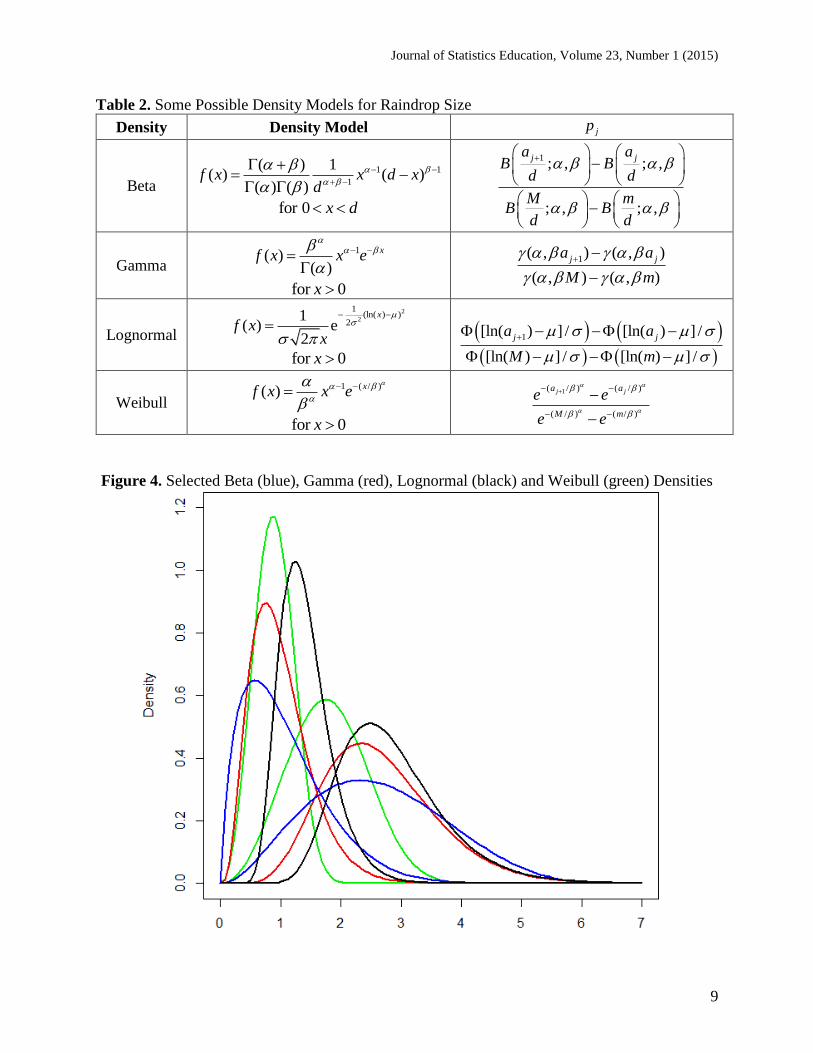
If a parametric model is to be fit to data, students first need to have some acquaintance with the
variety of density curves associated with a particular model. In Figure 4, for example, we see
several beta, gamma, lognormal and Weibull density curves.
Journal of Statistics Education, Volume 23, Number 1 (2015)
9
Table 2. Some Possible Density Models for Raindrop Size
Density Density Model jp
Beta
1 1
1
( ) 1( ) ( )
( ) ( )f x x d x
d
for 0 x d
1; , ; ,
; , ; ,
j ja aB B
d d
M mB B
d d
Gamma 1( )
( )
xf x x e
for 0x
1( , ) ( , )
( , ) ( , )
j ja a
M m
Lognormal
2
2
1(ln( ) )
21
( ) e2
x
f xx
for 0x
1[ln( ) ] / [ln( ) ] /
[ln( ) ] / [ln( ) ] /
j ja a
M m
Weibull
1 ( / )( ) xf x x e
for 0x
1( / ) ( / )
( / ) ( / )
j ja a
M m
e e
e e
Figure 4. Selected Beta (blue), Gamma (red), Lognormal (black) and Weibull (green) Densities

Journal of Statistics Education, Volume 23, Number 1 (2015)
10
Helpful Hint: Closure properties, such as sums of independent normal random
variables being normal, are typically discussed to some extent within a
mathematical statistics class. Worth pointing out in the context of our raindrop
diameter data is that sums of certain gamma random variables are gamma. More
specifically, if independent gamma random variables have a common scale
parameter , then the sum is also gamma. This suggests, for example, that if
consecutive time blocks of data appear to be well-modelled by the gamma, then
we may see the gamma well-models the pooled set of data within these blocks.
The beta, lognormal and Weibull do not enjoy such a closure property.
4. Usefulness of Parametric Models
Why bother fitting theoretical models to the raindrop size data? In this section we present two
situations in which having a theoretical model is useful.
The first situation in which a theoretical model for raindrop size is useful concerns obtaining
“smoothed” estimates of probability. Consider the histogram of 155 drop sizes recorded by the
Parsivel disdrometer in a one-minute period beginning at 15:44 shown in Figure 5. Twenty-one
drops, for example, are observed in the interval [1.000 mm, 1.125 mm]. Consequently, an
empirical estimate of the fraction of drops of this size occurring at the surface (under the
atmospheric conditions present) is 21/155 or about 0.135. Likewise, one observation falls in the
interval [2.500 mm, 3.000 mm] giving a probability estimate of 1/155, or about 0.00645. But
what about the interval [2.250 mm, 2.500 mm]? No observations fall in this interval and yet, do
we really want to estimate the chance of seeing a drop in this interval as zero when an even
larger drop has been observed? Assigning a positive chance to falling in this interval seems more
reasonable.
Helpful Hint: For those students without a mathematical statistics background, it
is enough to point out the empirical method of estimating probabilities given
above (e.g. 21/155 as an estimate of the chance of a drop between 1.000 mm and
1.125 mm), with the caveat that nonsensical empirical estimates (the zero
empirical chance above) may be improved by “smoothing-out” the histogram in
some fashion.

Journal of Statistics Education, Volume 23, Number 1 (2015)
11
Figure 5. One Minute of Huntsville Parsivel Disdrometer Data Starting at 15:44
By fitting a smooth density curve to our histogram we can obtain a nonzero probability estimate
of falling in the interval [2.250 mm, 2.500 mm]. We use a gamma model for purposes of
illustration. Using the maximum likelihood procedure discussed in the next section, a fitted
gamma density model is
1( ) , 0( )
xf x x e x
where ˆ 8.77MLE and ˆ 8.21MLE mm-1 (these values will appear in the R console
window after running the R script). Integrating the density over the appropriate regions we have,
to three significant digits, the following smoothed probability estimates
(1.000 1.125) 0.139P X
(2.250 2.500) 0.00234P X
(2.500 3.000) .000480P X
where X is the raindrop diameter. (The technical details are given in the next section, but a quick
summary is given here. The above probabilities may be computed as values of jp given in

Journal of Statistics Education, Volume 23, Number 1 (2015)
12
equation (1) of Section 5 and Table 2 where the incomplete gamma function is defined as
1
0( , ) ,
xtx t e dt m = 0.250 mm, M = 7.000 mm, with
ja and 1ja being the interval
boundaries, e.g. 2.250 mm and 2.500 mm, respectively.)
Note that the empirical and theoretical probability estimates closely agree for the interval [1.000
mm, 1.125 mm] (0.135 versus 0.139, respectively). Also, the empirically estimated chance of
falling in the interval [2.500 mm, 3.000 mm] is greater than the theoretically estimated chance of
falling in this interval (0.00645 versus 0.000480, respectively). That the theoretical value is so
much smaller (by roughly a factor of 13) is perhaps reasonable since the observation in this
interval may be considered to be an outlier. Finally, the chance of falling in the interval [2.250
mm, 2.500 mm] is raised from an empirical value of zero to a more reasonable (positive)
theoretical value of 0.00234.
Alternative Application: Fitting the raindrop data as described above may be
initially daunting to students because of the complicated integral expressions
involved. As a “warm-up” students may be asked to collect interarrival time data
– the gap in time between consecutive arrivals at a store entrance, a fast food
drive-up window, or an ATM. The first listed author has had success doing this in
class a number of times and has generally asked for students to observe at least
50 data points so students can get some sense of the interarrival time data by
viewing a histogram. Invariably, this interarrival data will closely follow an
exponential density. (This may be casually checked by inspecting a histogram and
looking for an exponential pattern. An additional check concerns looking to see if
the sample mean and sample standard deviation are “close” since the population
values are equal. A bit more sophisticated check concerns looking at whether an
exponential probability plot is linear.) Because the exponential density is easily
integrated in closed-form, the probability calculations are more transparent to
students. The exponential setting is also a bit simpler because it involves just a
single parameter rather than the two parameters needed for the densities used in
this article.
The gamma density model above is a parametric model as we assume a functional form for the
density up to two to be determined parameters and . Nonparametric models – models not
assuming a specific functional form, may also be used. Basically, these nonparametric models
attach a small “mound” centered at each data point. These mounds are added together to give a
model of the density function. Numeric integration of this density gives probability estimates
akin to those given above.
Helpful Hint: Such a nonparametric density estimate is referred to as a kernel
density estimate. The theory here is well-developed, with much of it concerned
with optimizing the shape and width of the mounds that are used with respect to
some measure of quality of fit. For further details see, for example, Scott (1992).
A second situation in which a parametric model for raindrop size is extremely useful concerns
precipitation algorithms such as those implemented by the Global Precipitation Measurement

Journal of Statistics Education, Volume 23, Number 1 (2015)
13
(GPM) Core Observatory. This satellite was successfully deployed by NASA and the Japan
Aerospace Exploration Agency on February 28, 2014 (c.f. http://gpm.nasa.gov/). At the risk of
over-simplifying the process, we now describe how GPM performs density estimation (more
details are given, for example, in Liao et al. 2005). One key equation concerns the equivalent
radar reflectivity factor, call it ,eZ of a radar operating at wavelength :
0( ) ( , ) ( )eZ c b x Nf x dx
Here, ( )c is a constant depending on the wavelength and the refractive index of water,
( , )b x is the raindrop “backscattering cross section,” N is the drop number concentration (drops
per unit volume of air), and ( )f x is the underlying density function of raindrop size, x. As eZ
may be estimated from measured radar return signals (“attenuation,” or loss of signal, is
involved) and both ( )c and ( , )b x are known, the only unknowns in the above equation are N
and the density function ( )f x for the drop size. This type of equation – an “inverse problem,” is
difficult to solve in general, but is made tractable by assuming the density has a particular
parametric form. In particular, a (two-parameter) gamma density model is currently assumed by
GPM. This gives us three unknown quantities to estimate. As the GPM Core Observatory
contains a dual-frequency precipitation radar looking at overlapping regions of the Earth, two
instances of the above equation may be obtained. A third empirical relation relating these three
parameters – which we will not elaborate on here, then gives the necessary three equations in
three unknowns to allow the unknown quantities to be estimated.
Once the raindrop size parameters are estimated, a handful of summary measures may be
computed from the fitted gamma model. These summaries include the rainfall rate, which has
some bearing on the global water balance, the likelihood of flooding and soil erosion, and the
liquid water content, which is related to the storm water balance and the distribution of latent
heat release in the clouds. (The rainfall rate and liquid water content are essentially computed as
different moments of the drop size distribution.)
It is important to note that algorithms used by the GPM are not fixed. In particular, “as
algorithms continue to mature and refine, GPM . . . will be updated and reprocessed . . .
throughout the GPM mission life” (Hou et al. 2014, p. 716). Such algorithm refinement is made
possible through “a broad range of joint projects with domestic and international partners to use
ground-based observations (including aircraft measurements) to conduct . . . validation
activities” (Hou et al. 2014, p. 714).
Consequently, an excellent area of research concerns the choice of parametric density functions
that should be used by GPM to model raindrop size. If just one collection of density functions is
used, is the gamma collection of densities “best”? Would another collection of density functions
generally perform “better”? Alternatively, should GPM not confine itself to a single collection of
densities and adaptively choose between different collections of density models from the
observed data?
To the best of our knowledge, GPM collects raindrop diameters over one-minute or sometimes
even shorter time intervals. So in the research investigation just mentioned, it would be

Journal of Statistics Education, Volume 23, Number 1 (2015)
14
appropriate to judge fit performance on individual minutes rather on consecutive blocks of
minutes with our data.
5. Maximum Likelihood Parameter Estimation for Truncated and Binned
Observations
The material in this section is appropriate for students in a mathematical statistics class who have
been exposed to maximum likelihood estimation. Instructors who have not discussed the
multinomial probability mass function with their students will want to briefly do so in
preparation for presentation of the material below.
Before getting into the complexities of the binned, truncated problem associated with our
disdrometer data, we suggest instructors present the maximum likelihood estimation of the two
parameters of at least one of the four densities listed in Table 2 in the continuous, untruncated
case. We very briefly outline such now for a random sample from a gamma density. If
1 2, ,..., nX X X is an independent sample from the gamma density function parameterized in Table
2, then from the likelihood L, defined as
1
1
( , )( )
i
nX
i
i
L X e
we obtain 1/n
1
1ln[ ( , )] ln ln ( ) ( 1) ln
n
i
i
L Xn
Setting the derivatives of this with respect to and equal to zero, and performing a bit of
algebra we obtain the two equations 1/n
1
' ( )ln ln
( )
n
i
i
X X
X
Solving the first equation (one method involves recursion, see for example Bowman and Shenton
1988) gives the maximum likelihood estimate of . The maximum likelihood estimate for
then follows from the second equation.
Suppose now that we have observed binned gamma data that has no (or little) truncation. A
tempting procedure would be to replace the bin counts with like numbers of values at bin
midpoints and then use the maximum likelihood procedure just outlined above. We, in fact,
encourage this kind of thinking from our students – we like them to solve new problems by
reducing them to frameworks in which solution techniques are already known. Unfortunately,
while this replacement of counts by midpoints works well in the case that the bins are very

Journal of Statistics Education, Volume 23, Number 1 (2015)
15
narrow, this approach in general leads to biased parameter estimates and, indeed, has been
labeled ‘crude’ by McLachlan and Krishnan (1997, p. 77).
We now discuss how to properly implement maximum likelihood parameter estimation for a
general binned, truncated situation. We then specialize to the beta, gamma, lognormal and
Weibull distributions listed in Table 2. As instructors present this material to their students we
suggest they emphasize two particular points made below: (1) the truncation problem leads to a
rescaling of the density over the region in which observations are collected (so that it integrates
to one) and (2) the chance of seeing a particular set of counts is just a multinomial problem,
albeit with very complicated probabilities.
If we take f as the density for drop size but we only observe drop sizes over the interval [m, M],
then
( )( ) ,
( ) ( )
f xf x m x M
F M F m
is the density for the truncated observations where 0
( ) ( ) ( )y y
F y f x dx f x dx
is the
cumulative distribution function. The truncated density, ( ) ( ; )f x f x , will depend upon any
unknown parameters which we indicate by (possibly a vector with more than one component).
For our binned situation, rather than seeing the actual observations, we are only able to count 1n
observations in 2 1 2[ , ] [ , ]m a a a , 2n observations in 2 3[ , ]a a , . . ., 1kn observations in 1[ , ]k ka a
and kn observations in 1[ , ] [ , ]k k ka a a M . The probability we see these counts is given by the
multinomial probability
1 2
1 2
1 2
!
! ! !
kn n n
k
k
np p p
n n n
where
1
( ) ( ; )j
j
a
j ja
p p f x dx
(1)
and 1
.k
i
i
n n
Consequently, the likelihood may be taken to be
1 2
1 2( ) knn n
kL p p p (2)
and we may find the maximum likelihood estimator by maximizing
: 0
ln( ( )) ln( ( ))
j
j j
j n
L n p
(3)
with respect to (c.f. Cowan 1998).

Journal of Statistics Education, Volume 23, Number 1 (2015)
16
The above general discussion may be specialized to the density models listed in Table 2. In
particular, to implement the maximum likelihood procedure mentioned above, it is enough to
specify ( )j jp p given in equations (2) and (3) for these models. These are given in the
rightmost column of Table 2 in terms of three special mathematical functions. Here,
1 1
0; , (1 ) ( , , )* ( , )
x
B x t t dt pbeta x beta
1
0( , ) ( , )* ( )
xtx t e dt pgamma x gamma ,
2 /21
( ) ( )2
xtx e dt pnorm x
are the incomplete beta, the incomplete gamma, and the standard normal cumulative distribution
functions, respectively (with R commands for their computation on the right-hand sides). The
maximization of the log likelihood in (3) is numerically intensive and may be accomplished
through the use of the optim( ) command in R via the script ML Rain.R accompanying this
article, available at:
http://www.amstat.org/publications/jse/v23n1/johnson/ML_Rain_16_Nov_2014.R
Students with some integration skill may be asked to verify the various jp entries in Table 2. As
indicated above, in each case the cumulative distribution F should first be computed to determine
the truncated distribution f from which integration over the thj bin gives .jp
Helpful Hint: Instructors might consider computing one of the expressions for jp
in Table 2 in class and then giving the remaining three (without knowledge of the
answers) as homework. Students can be told that access to the three special
mathematical functions is assumed (so that their answers may be expressed in
terms of these).
Helpful Hint: Observations from a known member of one of our four densities
may be generated via simulation and then truncated and binned. The maximum
likelihood estimates may then be computed and compared with the true values to
assess performance (e.g., with summaries such as the root mean squared error).
Estimate performance may be examined across different types of binning
including, but not necessarily limited to, our bins for the JW and Parsivel
disdrometers. Additionally, the performance of estimates obtained by replacing
counts by like numbers of midpoints may be assessed by simulation.
Alternative Application (Graduate Students): For students learning about the
Expectation-Maximization (EM) algorithm an alternative solution to finding
maximum likelihood estimates for our binned, truncated problem is stated in
general terms in Section 2.8 of McLachlan and Krishnan (1997). Such students
Journal of Statistics Education, Volume 23, Number 1 (2015)
17
can be asked to specialize this solution to one or more of our four densities.
(Details on the specialization to the gamma case are available from the first listed
author.)
6. Assessing Quality of Fit
“All models are wrong, but some are useful” – George Box (Box and Draper 1987)
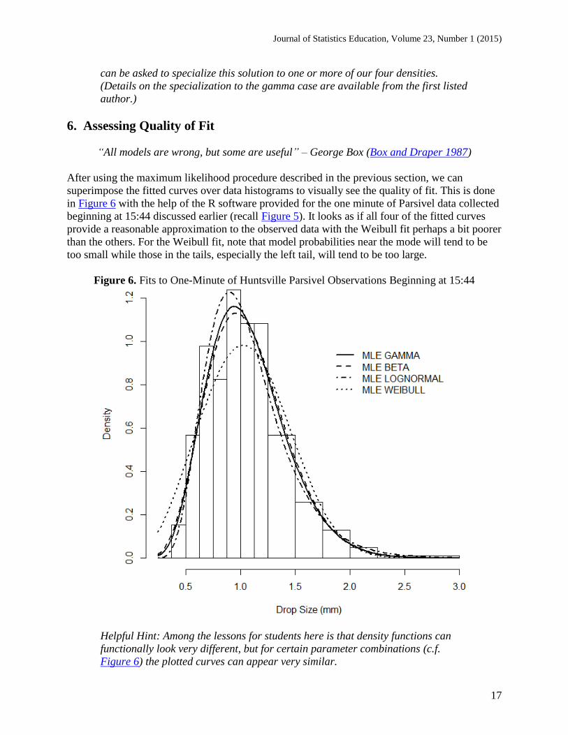
After using the maximum likelihood procedure described in the previous section, we can
superimpose the fitted curves over data histograms to visually see the quality of fit. This is done
in Figure 6 with the help of the R software provided for the one minute of Parsivel data collected
beginning at 15:44 discussed earlier (recall Figure 5). It looks as if all four of the fitted curves
provide a reasonable approximation to the observed data with the Weibull fit perhaps a bit poorer
than the others. For the Weibull fit, note that model probabilities near the mode will tend to be
too small while those in the tails, especially the left tail, will tend to be too large.
Figure 6. Fits to One-Minute of Huntsville Parsivel Observations Beginning at 15:44
Helpful Hint: Among the lessons for students here is that density functions can
functionally look very different, but for certain parameter combinations (c.f.
Figure 6) the plotted curves can appear very similar.

Journal of Statistics Education, Volume 23, Number 1 (2015)
18
How can we more objectively measure the quality of fit? One measure of quality of fit is
Pearson’s chi-squared goodness of fit (GOF) statistic; other suggested measures may be found,
for example, in D’Agostino and Stephens (1986). In the context of our problem, Pearson’s GOF
measure is given by 2
all bins
( )GOF i i
i
n e
e
where in is the observed count in the thi bin 1[ , ]i ia a and
1
( )i
i
a
ia
e n f x dx
is the expected count in the thi bin, n being the sum of all observed counts and f the density
over the truncated range of observations. Small GOF values indicate good agreement between
data and model, while large GOF values indicate poor agreement between data and model. To
rough approximation, the GOF measure has a chi-squared distribution with degrees of freedom
given by the number of bins minus the number of estimated parameters minus one. As each of
our four densities has two parameters to estimate, the degrees of freedom are given by the
number of bins minus 3.
Helpful Hint: The expected values in the above GOF statistic may be a bit
daunting to students since they involve rather complicated integrals. To build-up
some experience in the use of the GOF statistic, a less complicated setting may be
examined first. Students may, for example, investigate claims that Mars, Inc.
makes about its various M&M brands. For its Milk Chocolate variety they claim
24% of those manufactured are blue, 20% are orange, 16% are green, 14% are
yellow, 13% are red and 13% are brown. The degrees of freedom of the
approximating chi-squared distribution here is 6-1 = 5. Further details on doing
so using M&M candies may be found, for example, in Johnson (1993).
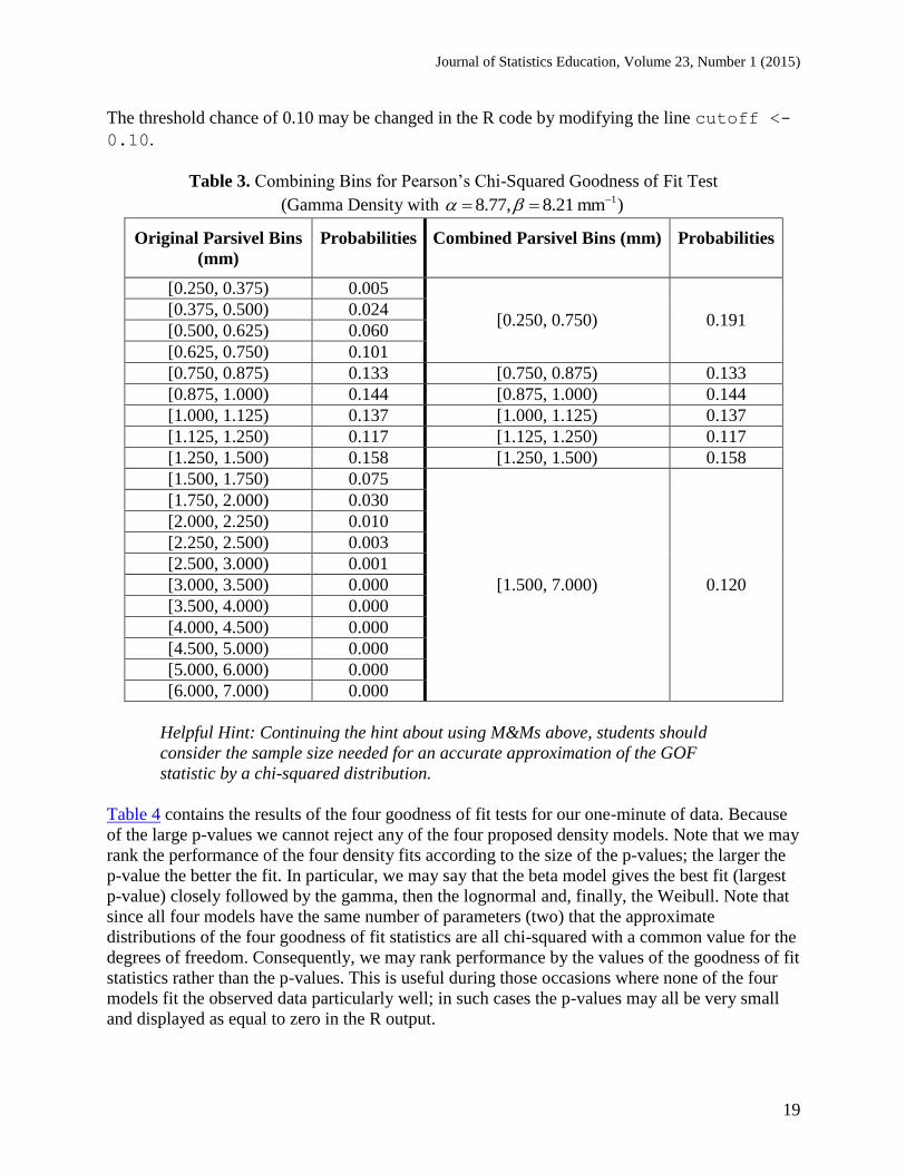
Unfortunately, this approximation is generally only considered good if the expected counts in
each bin are at least at some threshold; a value of 5 is often used. Consequently, we combine the
bins 1[ , ]i ia a to have a chance of at least 0.10 of containing an observation and suggest that
collections of raindrops at least 50 in number be used to achieve the expected count of 5 in each
bin. Some elaboration is in order. For the 155 Parsivel observations starting at 15:44, a gamma
density was fit giving the estimated values 18.77, 8.21 mm . Starting with the smallest
bin of [0.250 mm, 0.375 mm], since the chance of falling in this bin is less than 0.10 – it is about
0.005, we combine this bin with additional contiguous larger bins until the cumulative chance is
at least 0.10. As shown in Table 3 the smallest four bins are combined into the single bin [0.250
mm, 0.750 mm] to achieve a chance of 0.191. In our example, none of the next five bins needs to
be combined as each has an associated chance of at least 0.10. We continue this process moving
from left-to-right across the bins, combining as necessary so that there is at least 0.10 chance of
falling in each bin. For the sake of a uniform set of bins across the four goodness of fit
calculations, we use the combined bins determined by the gamma fit for all four density models.
Journal of Statistics Education, Volume 23, Number 1 (2015)
19
The threshold chance of 0.10 may be changed in the R code by modifying the line cutoff <-
0.10.
Table 3. Combining Bins for Pearson’s Chi-Squared Goodness of Fit Test
(Gamma Density with 18.77, 8.21 mm )
Original Parsivel Bins
(mm)
Probabilities Combined Parsivel Bins (mm) Probabilities
[0.250, 0.375) 0.005
[0.250, 0.750) 0.191 [0.375, 0.500) 0.024
[0.500, 0.625) 0.060
[0.625, 0.750) 0.101
[0.750, 0.875) 0.133 [0.750, 0.875) 0.133
[0.875, 1.000) 0.144 [0.875, 1.000) 0.144
[1.000, 1.125) 0.137 [1.000, 1.125) 0.137
[1.125, 1.250) 0.117 [1.125, 1.250) 0.117
[1.250, 1.500) 0.158 [1.250, 1.500) 0.158
[1.500, 1.750) 0.075
[1.500, 7.000) 0.120
[1.750, 2.000) 0.030
[2.000, 2.250) 0.010
[2.250, 2.500) 0.003
[2.500, 3.000) 0.001
[3.000, 3.500) 0.000
[3.500, 4.000) 0.000
[4.000, 4.500) 0.000
[4.500, 5.000) 0.000
[5.000, 6.000) 0.000
[6.000, 7.000) 0.000
Helpful Hint: Continuing the hint about using M&Ms above, students should
consider the sample size needed for an accurate approximation of the GOF
statistic by a chi-squared distribution.
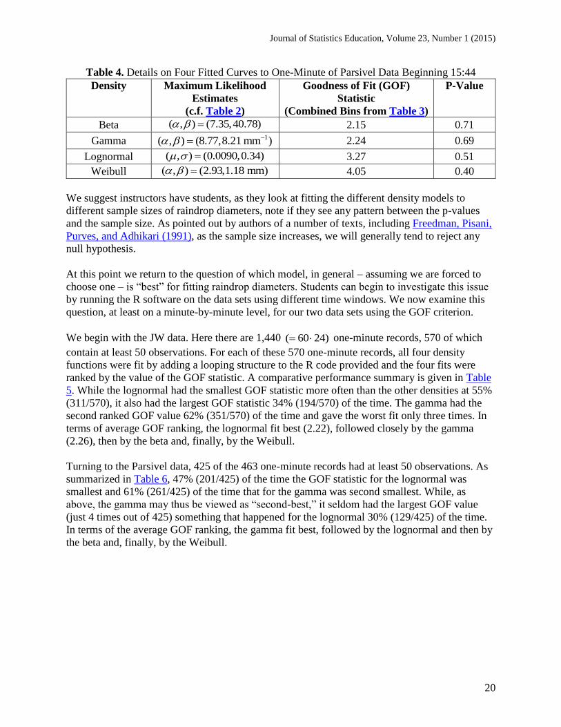
Table 4 contains the results of the four goodness of fit tests for our one-minute of data. Because
of the large p-values we cannot reject any of the four proposed density models. Note that we may
rank the performance of the four density fits according to the size of the p-values; the larger the
p-value the better the fit. In particular, we may say that the beta model gives the best fit (largest
p-value) closely followed by the gamma, then the lognormal and, finally, the Weibull. Note that
since all four models have the same number of parameters (two) that the approximate
distributions of the four goodness of fit statistics are all chi-squared with a common value for the
degrees of freedom. Consequently, we may rank performance by the values of the goodness of fit
statistics rather than the p-values. This is useful during those occasions where none of the four
models fit the observed data particularly well; in such cases the p-values may all be very small
and displayed as equal to zero in the R output.
Journal of Statistics Education, Volume 23, Number 1 (2015)
20
Table 4. Details on Four Fitted Curves to One-Minute of Parsivel Data Beginning 15:44
Density Maximum Likelihood
Estimates
(c.f. Table 2)
Goodness of Fit (GOF)
Statistic
(Combined Bins from Table 3)
P-Value
Beta ( , ) (7.35,40.78) 2.15 0.71
Gamma 1( , ) (8.77,8.21 mm ) 2.24 0.69
Lognormal ( , ) (0.0090,0.34) 3.27 0.51
Weibull ( , ) (2.93,1.18 mm) 4.05 0.40
We suggest instructors have students, as they look at fitting the different density models to
different sample sizes of raindrop diameters, note if they see any pattern between the p-values
and the sample size. As pointed out by authors of a number of texts, including Freedman, Pisani,
Purves, and Adhikari (1991), as the sample size increases, we will generally tend to reject any
null hypothesis.
At this point we return to the question of which model, in general – assuming we are forced to
choose one – is “best” for fitting raindrop diameters. Students can begin to investigate this issue
by running the R software on the data sets using different time windows. We now examine this
question, at least on a minute-by-minute level, for our two data sets using the GOF criterion.
We begin with the JW data. Here there are 1,440 ( 60 24) one-minute records, 570 of which
contain at least 50 observations. For each of these 570 one-minute records, all four density
functions were fit by adding a looping structure to the R code provided and the four fits were
ranked by the value of the GOF statistic. A comparative performance summary is given in Table
5. While the lognormal had the smallest GOF statistic more often than the other densities at 55%
(311/570), it also had the largest GOF statistic 34% (194/570) of the time. The gamma had the
second ranked GOF value 62% (351/570) of the time and gave the worst fit only three times. In
terms of average GOF ranking, the lognormal fit best (2.22), followed closely by the gamma
(2.26), then by the beta and, finally, by the Weibull.
Turning to the Parsivel data, 425 of the 463 one-minute records had at least 50 observations. As
summarized in Table 6, 47% (201/425) of the time the GOF statistic for the lognormal was
smallest and 61% (261/425) of the time that for the gamma was second smallest. While, as
above, the gamma may thus be viewed as “second-best,” it seldom had the largest GOF value
(just 4 times out of 425) something that happened for the lognormal 30% (129/425) of the time.
In terms of the average GOF ranking, the gamma fit best, followed by the lognormal and then by
the beta and, finally, by the Weibull.

Journal of Statistics Education, Volume 23, Number 1 (2015)
21
Table 5. Ranking of Fits for the One-Minute JW Intervals
Density Average
GOF Rank
Times GOF Ranked . . .
First
(Smallest GOF)
Second Third Fourth
(Largest GOF)
Beta 2.49 52 192 322 4
Gamma 2.26 37 351 179 3
Lognormal 2.22 311 17 48 194
Weibull 3.03 170 10 21 369
Table 6. Ranking of Fits for One-Minute Parsivel Intervals
Density Average
GOF Rank
Times GOF Ranked . . .
First
(Smallest GOF)
Second Third Fourth
(Largest GOF)
Beta 2.37 68 141 207 9
Gamma 2.20 42 261 118 4
Lognormal 2.32 201 16 79 129
Weibull 3.11 114 7 21 283
Comparing Tables 5 and 6 we note that the relative performance among the four densities is
quite similar across the two data sets.
While the beta and Weibull can provide good fits to raindrop diameters, the beta typically is third
and the Weibull is generally fourth (last) in the GOF rankings. Consequently, the choice of a best
density seems to be between the lognormal and the gamma. While the lognormal performs best
most often, it also ranks last among the four densities a large percentage of the time.
Accordingly, the gamma density may be argued as the best among the four densities.
Running the ML Rain code allows students to examine curve fitting performance for intervals
larger than one-minute intervals. Such longer intervals are sometimes used to facilitate
comparisons between disdrometer and rain-gauge data; the gauges often require longer periods to
accumulate enough rain to permit suitable accuracy in the measurements.
Helpful Hint: Instructors who like to incorporate writing into their classes may
give a homework assignment in which students (e.g. in groups of two or three), in
a report addressed to GPM scientists, either argue for the single best collection of
densities that should be used or for a particular adaptive procedure for selecting
a particular collection of densities. Their arguments should be supported by
numeric and graphic output produced by the R code provided.
Helpful Hint: Instructors of students not having a mathematical statistics
background may still find the above material useful. In particular, instructors
may give the observed and expected counts for all four of our density models (this
information is output by the R code) with respect to some subset of the data and
then ask students to say which density model fits best. The instructor in this case

Journal of Statistics Education, Volume 23, Number 1 (2015)
22
can skip any discussion of maximum likelihood and, in fact, can relay the needed
information from the R code so that the students do not even need to run it.
7. Initial Estimates to Start Maximum Likelihood Estimation
A complicating issue which would have possibly detracted from the discussion above is now
briefly discussed in this section. This issue may provide ideas to instructors about possible
student research projects.
The maximization performed in the R code to find maximum likelihood estimates is done using
the optim( ) function. We implement this function with the default algorithm due to Nelder and
Mead (1965). A required input to the optim( ) function is an initial guess of the parameter values.
The code provided uses fixed rather than data-driven initial estimates of the parameters of each
of our four densities. If we had continuous observations, rather than counts, from the untruncated
densities listed in Table 2, then method of moments could be used to easily provide data-driven
initial estimates. If X and 2s denote the sample mean and sample variance from the gamma
density with the parametrization from Table 2, for example, then these two sample values could
replace the population values in the expressions
2
2( ) , ( )E X Var X
to obtain the estimates 2
2 2ˆˆ ,
X X
s s
Unfortunately, the rescaled densities that arise because of the truncation (the densities f from
Section 5) give rise to highly nonlinear expressions for the first two moments that do not lead to
easily solved method of moments estimates. A plausible way around this for the two data sets
provided with this article, if the truncation is slight, is to use the above method of moments
procedure upon replacing counts by like numbers of observations at, say, bin midpoints. The
authors, however, have found limited success with this approach. In simulations in which
parameter values are known, this approach often leads to initial parameter estimates far from the
true values even for an apparently small amount of truncation.
The good news, with respect to the fits performed on the 570 one-minute JW records and the 425
one-minute Parsivel records in the previous section, was that R indicated convergence for each
of these one-minute observations for all four density models. The bad news is that the
convergence, at times, may be to local extrema rather than global extrema. There is some change
– quite limited, but nonetheless change, to the results in Tables 5 and 6 when the initial fixed
starting values are changed.
Helpful Hint: A possible research question would be to find initial estimates,
hopefully simple, to start a nonlinear optimization search for the maximum
likelihood estimates that improves upon starting with fixed initial values. Unless
truncation is quite severe, the mode of the original untruncated density and the
truncated density should be the same (as the mode is not affected by the scaling
due to truncation). This seems to provide one useful constraint on a problem

Journal of Statistics Education, Volume 23, Number 1 (2015)
23
involving the estimation of two unknowns for any one of our four densities. An
additional constraint would thus be needed to estimate our two unknowns.
Alternative Application (Graduate Students): Sheppard’s corrections (see, for
example, Stuart and Ord 1994) are used to correct for bias when using sample
moments of binned data to estimate population moments. Students may be asked
to research these corrections and indicate why the assumptions needed for their
use are not satisfied by any of our four density models.
8. Summary
How large and how variable are raindrops in size? How does size vary from storm to storm?
How can we characterize the distribution shape of raindrop sizes? What is the probability of
seeing a raindrop diameter between two specified values? Accompanying this article are data
sets containing measurements of raindrop diameters collected from both the Kwajalein Atoll in
the northern Pacific and Huntsville, AL. Students can begin to investigate answers to the
questions just posed, at least under similar atmospheric conditions, through basic exploratory
data analysis with the R script provided.
In some contexts, such as obtaining “smoothed” estimates to the probability question stated
above, as well as characterizing raindrop size distributions for use with the Global Precipitation
Measurement (GPM) Observatory, it is useful to model raindrop distributions parametrically. As
raindrop size is typically unimodal and skewed to the right, members of the beta, gamma,
lognormal and Weibull densities may be considered as potential models. Parameter estimation
using maximum likelihood – maximum likelihood being a technique that generally outperforms
other estimation techniques, is difficult in our setting as disdrometer data are both truncated and
binned. Such complications in a real world setting provide a richness to classroom discussion of
parameter estimation in general, and maximum likelihood estimation in particular, within
mathematical statistics courses or courses which have mathematical statistics as a prerequisite.
The R script provided produces parameter estimates using maximum likelihood and assesses the
quality of fit both graphically – by superimposing the fitted curves over histograms of the
underlying raindrop diameters, and numerically – through the generation of a goodness of fit
statistic.
Further elaboration of fitting raindrop diameters, including by the L-moments technique
(Hosking 1990), may be found in a series of articles written by the authors (Kliche, Smith and
Johnson 2008, Smith, Kliche and Johnson 2009, Johnson, Kliche and Smith 2011 and Johnson,
Kliche and Smith 2014). The article by Johnson et al. 2014 includes simulation of drop sizes
from a known gamma distribution so as to examine the accuracy of maximum likelihood
parameter estimates in the binned, truncated case we have discussed in this article.
Additional disdrometer data, as it becomes available, will be placed at the Website
http://www.mcs.sdsmt.edu/rwjohnso/html/disdrometer data.html. The second listed author, in
particular, has two Parsivel disdrometers that are now deployed in western South Dakota.

Journal of Statistics Education, Volume 23, Number 1 (2015)
24
Acknowledgements
The Parsivel disdrometer data were kindly provided courtesy of Dr. Walt Petersen while he was
associated with the Earth System Science Center, National Space Science and Technology
Center, University of Alabama, Huntsville. The Kwajalein Atoll disdrometer data were kindly
provided courtesy of the US Army Space Missile Defense Command Reagan Test Site, NASA
Goddard Space Flight Center, and Atmospheric Technology Services Co.
References
Alonge, A. and Afullo, T. (2012), “Seasonal analysis and prediction of rainfall effects in eastern
South Africa at microwave frequencies,” Progress in Electromagnetics Research, 40:279-303.
Bardsley, W. (2007), “Note on y-truncation: A simple approach to generating bounded
distributions for environmental applications,” Advances in Water Resources, 30(1):113-117.
Bowman, K. and Shenton, L. (1988), Properties of Estimators for the Gamma Distribution, New
York, NY: Marcel Dekker.
Box, G. and Draper, N. (1987), Empirical Model-Building and Response Surfaces, p. 424, New
York, NY: John Wiley & Sons.
Brawn, D. and Upton, G. (2007), “Closed-form parameter estimates for a truncated gamma
distribution,” Environmetrics, 18(6):633-645.
Brawn, D. and Upton, G. (2008), “Estimation of an atmospheric gamma drop size distribution
using disdrometer data,” Atmospheric Research, 87(1):66-79.
Chandrasekar, V. and Bringi, V.N. (1987), “Simulation of radar reflectivity and surface
measurements of rainfall,” Journal of Atmospheric and Oceanic Technology, 4(3):464-478.
Cowan, G. (1998), Statistical Data Analysis, Oxford, UK: Clarendon Press.
D’Agostino, R. and Stephens, M. (1986), Goodness-of-Fit Techniques, New York, NY: Marcel
Dekker.
Feingold, G. and Levin, Z. (1986), “The lognormal fit to raindrop spectra from frontal
convective clouds in Israel,” Journal of Climate and Applied Meteorology, 25(10):1346-1363.
Freedman, D., Pisani, R., Purves, R. and Adhikari, A. (1991), Statistics, 2nd edition, New York,
NY: W.W. Norton.
Hosking, J.R.M. (1990), “L-moments: Analysis and estimation of distributions using linear
combinations of order statistics,” Journal of the Royal Statistical Society, Series A, B52:105-124.

Journal of Statistics Education, Volume 23, Number 1 (2015)
25
Hou, A., Kakar, R., Neeck, S., Azarbarzin, A., Kummerow, C., Kojima, M., Oki, R., Nakamura,
K. and Iguchi, T. (2014), “The global precipitation measurement mission,” Bulletin of the
American Meteorological Society, May issue, 701-722.
Johnson, R. (1993), “Testing colour proportions of M&Ms,” Teaching Statistics, 15(1):2-4.
Johnson, R., Kliche, D. and Smith, P. (2011), “Comparison of estimators for parameters of
gamma distributions with left-truncated samples,” Journal of Applied Meteorology and
Climatology, 50(2):296-310.
Johnson, R., Kliche, D. and Smith, P. (2014), “Maximum likelihood estimation of gamma
parameters for coarsely-binned and truncated raindrop size data,” Quarterly Journal of the Royal
Meteorological Society, 140(681):1245-1256.
Kliche, D. (2007), Raindrop Size Distribution Functions: An Empirical Approach, Ph.D.
dissertation, South Dakota School of Mines & Technology, Atmospheric Sciences Department,
197pp.
Kliche, D., Smith, P. and Johnson, R. (2008), “L-moment estimators as applied to gamma drop
size distributions,” Journal of Applied Meteorology and Climatology, 47(12):3117-3130.
Liao, L., Meneghini, R., Iguchi, T. and Detwiler, A. (2005), “Use of dual-wavelength radar for
snow parameter estimates,” Journal of Atmospheric and Oceanic Technology, 22(10):1494-1506.
Löffler-Mang, M. and Joss, J. (2000), “An optical disdrometer for measuring size and velocity of
hydrometeors,” Journal of Atmospheric and Oceanic Technology, 17(2):130-139.
Marshall, J.S. and Palmer W.M. (1948), “The distribution of raindrops with size,” Journal of
Meteorology, 5(4):165-166.
McLachlan, G. and Krishnan, T. (1997), The EM Algorithm and Extensions, New York, NY:
John Wiley & Sons.
Nelder, J. and Mead, R. (1965), “A simplex algorithm for function minimization,” Computer
Journal, 7(4):308-313.
R Development Core Team (2013), R: A Language and Environment for Statistical Computing,
ISBN 3-900051-07-0, Vienna, Austria: R Foundation for Statistical Computing. Available at
http://www.R-project.org.
Scott, D. (1992), Multivariate Density Estimation: Theory, Practice, and Visualization, New
York, NY: John Wiley & Sons.
Smith, P., Kliche, D. and Johnson, R. (2009), “The bias and error in moment estimators for
parameters of drop-size distribution functions: Sampling from gamma distributions,” Journal of
Applied Meteorology and Climatology, 48(10):2118-2126.
Journal of Statistics Education, Volume 23, Number 1 (2015)
26
Stuart, A. and Ord J.K. (1994), Kendall’s Advanced Theory of Statistics, Distribution Theory 1,
6th edition, London, UK: Edward Arnold.
Tokay, A., Bashor, P. and Wolff, K.R. (2005), “Error characteristics of rainfall measurements by
collocated Joss-Waldvogel disdrometers,” Journal of Atmospheric and Oceanic Technology,
22(5):513-527.
Ulbrich, C.W. (1983), “Natural variations in the analytical form of the raindrop size
distribution,” Journal of Climate and Applied Meteorology, 22(10):1764-1775.
Villermaux, E. and Bossa, B. (2009), “Single-drop fragmentation determines size distribution of
raindrops,” Nature Physics, 5:697-702.
Roger W. Johnson
Department of Mathematics and Computer Science
South Dakota School of Mines & Technology
Rapid City, SD 57701
Donna V. Kliche
Atmospheric and Environmental Sciences Program
South Dakota School of Mines & Technology
Rapid City, SD 57701
Paul L. Smith
Atmospheric and Environmental Sciences Program
South Dakota School of Mines & Technology
Rapid City, SD 57701
Volume 23 (2015) | Archive | Index | Data Archive | Resources | Editorial Board | Guidelines for
Authors | Guidelines for Data Contributors | Guidelines for Readers/Data Users | Home Page |
Contact JSE | ASA Publications