Modeling Purposeful Adaptive Behavior with the Principle ...
236
Modeling Purposeful Adaptive Behavior with the Principle of Maximum Causal Entropy Brian D. Ziebart December 2010 CMU-ML-10-110 Machine Learning Department School of Computer Science Carnegie Mellon University Pittsburgh, PA 15213 Thesis Committee J. Andrew Bagnell, Co-chair Anind K. Dey, Co-chair Martial Hebert Dieter Fox, University of Washington Submitted in partial fulfillment of the requirements for the degree of Doctor of Philosophy c 2010 Brian D. Ziebart This research was sponsored by an R. K. Mellon Fellowship and by the National Science Foundation under contract no. EEEC-0540865. The views and conclusions contained in this document are those of the author and should not be interpreted as representing the official policies, either expressed or implied, of any sponsoring institution, the U.S. government or any other entity.
Transcript of Modeling Purposeful Adaptive Behavior with the Principle ...

Modeling Purposeful Adaptive Behavior withthe Principle of Maximum Causal Entropy
Brian D. Ziebart
December 2010CMU-ML-10-110
Machine Learning DepartmentSchool of Computer ScienceCarnegie Mellon University
Pittsburgh, PA 15213
Thesis CommitteeJ. Andrew Bagnell, Co-chair
Anind K. Dey, Co-chairMartial Hebert
Dieter Fox, University of Washington
Submitted in partial fulfillment of the requirementsfor the degree of Doctor of Philosophy
c© 2010 Brian D. Ziebart
This research was sponsored by an R. K. Mellon Fellowship and by the National Science Foundation undercontract no. EEEC-0540865. The views and conclusions contained in this document are those of the author and shouldnot be interpreted as representing the official policies, either expressed or implied, of any sponsoring institution, theU.S. government or any other entity.

Keywords: Machine learning, decision making, probabilistic modeling, maximum entropy,inverse optimal control, influence diagrams, informational revelation, feedback, causality, goalinference

Abstract
Predicting human behavior from a small amount of training examples is a challenging machinelearning problem. In this thesis, we introduce the principle of maximum causal entropy, a gen-eral technique for applying information theory to decision-theoretic, game-theoretic, and controlsettings where relevant information is sequentially revealed over time. This approach guaran-tees decision-theoretic performance by matching purposeful measures of behavior (Abbeel & Ng,2004), and/or enforces game-theoretic rationality constraints (Aumann, 1974), while otherwise be-ing as uncertain as possible, which minimizes worst-case predictive log-loss (Grunwald & Dawid,2003).
We derive probabilistic models for decision, control, and multi-player game settings using thisapproach. We then develop corresponding algorithms for efficient inference that include relax-ations of the Bellman equation (Bellman, 1957), and simple learning algorithms based on con-vex optimization. We apply the models and algorithms to a number of behavior prediction tasks.Specifically, we present empirical evaluations of the approach in the domains of vehicle routepreference modeling using over 100,000 miles of collected taxi driving data, pedestrian motionmodeling from weeks of indoor movement data, and robust prediction of game play in stochasticmulti-player games.


For Emily


Acknowledgments
I owe much gratitude to many people for their support and encouragement leading to this thesis.First and foremost, I thank my thesis advisors, Anind Dey and Drew Bagnell, for directing myresearch towards exciting problems and applications, and for supplying me with enough guidanceand knowledge to stay on the right path, but also enough freedom to feel empowered by the journey.I also thank Martial Hebert and Dieter Fox for serving on my thesis committee and providing theirvaluable insights on my research.
Many thanks go to the Quality of Life Technology Center (National Science Foundation GrantNo. EEEC-0540865) and the R.K. Mellon Foundation for supporting this research and the broadergoal of creating assistive technologies for those who would benefit from them.
I am indebted to Roy Campbell and Dan Roth for advising my initial experiences with computerscience research at the University of Illinois, as well as Manuel Roman and the rest of the SystemsResearch Group, for taking me in and making my experience enjoyable. That work continues tomotivate my thinking.
Without Eric Oatneal and Jerry Campolongo of Yellow Cab Pittsburgh, and Maury Fey ofWestinghouse SURE, our data collections and studies of driver preferences would not have beenpossible.
I thank my co-authors with whom I had the pleasure of working on the Purposeful PeoplePrediction project at Carnegie Mellon/Intel: Nathan Ratliff, Garratt Gallagher, Christoph Mertz,Sidd Srinivasa, and Kevin Peterson. Making robots reason and function purposefully is definitelya team activity.
Being a member of the Machine Learning Department (and the wider SCS and CMU commu-nity) has been a wonderful experience. I thank the faculty, the students, and the staff for making ita collegial and intellectually stimulating environment for learning and exploring this exciting field.Special thanks go to Andrew Arnold, Anind’s research group, Andy Carlson, Lucia Castellanos,Hao Cen, Miro Dudık, Joey Gonzalez, Sue Ann Hong, Jonathan Huang, Andreas Krause, LairLab,Thomas LaToza, Jure Leskovec, Mary McGlohon, Abe Othman, and Diane Stidle.
I thank my officemates over the years—Hao Cen, Robert Fisher, Hai-Son Le, Jonathan Moody,and Ankur Parikh—who were patient when maximizing entropy extended beyond my research tomy desk.
I thank Andrew Maas for his late night coding, ideas, karaoke singing, and friendship in ourendeavors together.
vii

viii
My former housemates Jure Leskovec, Andrew Arnold, and Thomas LaToza, made the transi-tion to Pittsburgh and Carnegie Mellon a pleasant one filled with cookies and a more than occa-sional games of Settlers of Catan.
To my parents: nature or nurture, I owe both to you. I thank you and my sister, Sarah, forfueling my curiosity, valuing my education, and for making me the person who I am today.
To my wife, Emily, your patience and support through the ups and downs of the research cyclehave been instrumental.

Contents
I Preliminaries 1
1 Introduction 21.1 Contributions to the Theory of Behavior Prediction . . . . . . . . . . . . . . . . . 41.2 Motivation . . . . . . . . . . . . . . . . . . . . . . . . . . . . . . . . . . . . . . . 51.3 Purposefulness, Adaptation, and Rationality . . . . . . . . . . . . . . . . . . . . . 51.4 Prescriptive Versus Predictive Models . . . . . . . . . . . . . . . . . . . . . . . . 91.5 Maximum Causal Entropy . . . . . . . . . . . . . . . . . . . . . . . . . . . . . . 91.6 Applications and Empirical Evaluations . . . . . . . . . . . . . . . . . . . . . . . 101.7 Thesis Organization and Reader’s Guide . . . . . . . . . . . . . . . . . . . . . . . 11
2 Background and Notation 152.1 Probabilistic Graphical Models . . . . . . . . . . . . . . . . . . . . . . . . . . . . 15
2.1.1 Bayesian Networks . . . . . . . . . . . . . . . . . . . . . . . . . . . . . . 152.1.2 Markov and Conditional Random Fields . . . . . . . . . . . . . . . . . . . 16
2.2 Decision-Theoretic Models . . . . . . . . . . . . . . . . . . . . . . . . . . . . . . 182.2.1 Markov Decision Processes . . . . . . . . . . . . . . . . . . . . . . . . . . 182.2.2 Linear-Quadratic Control . . . . . . . . . . . . . . . . . . . . . . . . . . . 212.2.3 Influence Diagrams . . . . . . . . . . . . . . . . . . . . . . . . . . . . . . 22
2.3 Notation and Terminology . . . . . . . . . . . . . . . . . . . . . . . . . . . . . . 252.4 Summary . . . . . . . . . . . . . . . . . . . . . . . . . . . . . . . . . . . . . . . 26
3 Related Work 273.1 Probabilistic Graphical Models for Decision Making . . . . . . . . . . . . . . . . 27
3.1.1 Directed Graphical Model Approaches . . . . . . . . . . . . . . . . . . . . 283.1.2 Undirected Graphical Approaches . . . . . . . . . . . . . . . . . . . . . . 31
3.2 Optimal Control Approaches . . . . . . . . . . . . . . . . . . . . . . . . . . . . . 313.2.1 Inverse Optimal Control . . . . . . . . . . . . . . . . . . . . . . . . . . . 323.2.2 Feature Matching Optimal Policy Mixtures . . . . . . . . . . . . . . . . . 323.2.3 Maximum Margin Planning . . . . . . . . . . . . . . . . . . . . . . . . . 353.2.4 Game-Theoretic Criteria . . . . . . . . . . . . . . . . . . . . . . . . . . . 363.2.5 Boltzmann Optimal-Action-Value Distribution . . . . . . . . . . . . . . . 36
ix

x CONTENTS
3.2.6 Robust and Approximate Optimal Control . . . . . . . . . . . . . . . . . . 373.2.7 Noise-Augmented Optimal Actions . . . . . . . . . . . . . . . . . . . . . 38
3.3 Discrete Choice Theory . . . . . . . . . . . . . . . . . . . . . . . . . . . . . . . . 393.3.1 Multinomial and Conditional Logit . . . . . . . . . . . . . . . . . . . . . . 393.3.2 Criticisms of the Independence of Irrelevant Alternatives Axiom . . . . . . 403.3.3 Nested Logit . . . . . . . . . . . . . . . . . . . . . . . . . . . . . . . . . 40
3.4 Discussion . . . . . . . . . . . . . . . . . . . . . . . . . . . . . . . . . . . . . . . 403.4.1 Connections Between Approaches . . . . . . . . . . . . . . . . . . . . . . 403.4.2 Relation to Thesis Contributions . . . . . . . . . . . . . . . . . . . . . . . 41
II Theory 43
4 The Theory of Causal Information 454.1 Information Theory . . . . . . . . . . . . . . . . . . . . . . . . . . . . . . . . . . 45
4.1.1 Entropy and Information . . . . . . . . . . . . . . . . . . . . . . . . . . . 454.1.2 Properties . . . . . . . . . . . . . . . . . . . . . . . . . . . . . . . . . . . 484.1.3 Information Theory and Gambling . . . . . . . . . . . . . . . . . . . . . . 49
4.2 Causal Information . . . . . . . . . . . . . . . . . . . . . . . . . . . . . . . . . . 504.2.1 Sequential Information Revelation and Causal Influence . . . . . . . . . . 504.2.2 Causally Conditioned Probability . . . . . . . . . . . . . . . . . . . . . . . 504.2.3 Causal Entropy and Information . . . . . . . . . . . . . . . . . . . . . . . 514.2.4 Properties . . . . . . . . . . . . . . . . . . . . . . . . . . . . . . . . . . . 524.2.5 Previous Applications of Causal Information . . . . . . . . . . . . . . . . 53
4.3 Discussion . . . . . . . . . . . . . . . . . . . . . . . . . . . . . . . . . . . . . . . 55
5 The Principle of Maximum Causal Entropy 565.1 Principle of Maximum Entropy . . . . . . . . . . . . . . . . . . . . . . . . . . . . 56
5.1.1 Justifications for the Principle of Maximum Entropy . . . . . . . . . . . . 575.1.2 Generalizations of the Principle of Maximum Entropy . . . . . . . . . . . 595.1.3 Probabilistic Graphical Models as Entropy Maximization . . . . . . . . . . 595.1.4 Approximate Constraints and Bayesian Inference . . . . . . . . . . . . . . 60
5.2 Maximum Causal Entropy . . . . . . . . . . . . . . . . . . . . . . . . . . . . . . 615.2.1 Convex Optimization . . . . . . . . . . . . . . . . . . . . . . . . . . . . . 625.2.2 Convex Duality . . . . . . . . . . . . . . . . . . . . . . . . . . . . . . . . 635.2.3 Worst-Case Predictive Guarantees . . . . . . . . . . . . . . . . . . . . . . 645.2.4 Gambling Growth Rate Guarantees . . . . . . . . . . . . . . . . . . . . . . 64
5.3 Information-Theoretic Extensions and Special Cases . . . . . . . . . . . . . . . . 655.3.1 Static Conditioning Extension . . . . . . . . . . . . . . . . . . . . . . . . 655.3.2 Optimizing Relative Causal Entropy . . . . . . . . . . . . . . . . . . . . . 665.3.3 Continuous-Valued Maximum Causal Entropy . . . . . . . . . . . . . . . . 67

CONTENTS xi
5.3.4 Deterministic Side Information . . . . . . . . . . . . . . . . . . . . . . . . 685.4 Discussion . . . . . . . . . . . . . . . . . . . . . . . . . . . . . . . . . . . . . . . 68
6 Statistic-Matching Maximum Causal Entropy 706.1 Statistic Matching Constraints . . . . . . . . . . . . . . . . . . . . . . . . . . . . 71
6.1.1 General and Control Motivations and Problem Setting . . . . . . . . . . . . 716.1.2 Optimization and Policy Form . . . . . . . . . . . . . . . . . . . . . . . . 716.1.3 Properties . . . . . . . . . . . . . . . . . . . . . . . . . . . . . . . . . . . 736.1.4 Markovian Simplifications . . . . . . . . . . . . . . . . . . . . . . . . . . 746.1.5 Goal-Directed Feature Constraints . . . . . . . . . . . . . . . . . . . . . . 75
6.2 Inverse Optimal Control . . . . . . . . . . . . . . . . . . . . . . . . . . . . . . . . 756.2.1 Policy Guarantees . . . . . . . . . . . . . . . . . . . . . . . . . . . . . . . 766.2.2 Soft Bellman Equation Interpretation . . . . . . . . . . . . . . . . . . . . . 766.2.3 Large Deviation Bounds . . . . . . . . . . . . . . . . . . . . . . . . . . . 796.2.4 Continuous Problems with Linear Dynamics and Quadratic Utilities . . . . 806.2.5 Deterministic Dynamics Reduction . . . . . . . . . . . . . . . . . . . . . . 81
6.3 Relation to Alternate Information-Theoretic Approaches . . . . . . . . . . . . . . 816.3.1 Maximum Joint Entropy . . . . . . . . . . . . . . . . . . . . . . . . . . . 826.3.2 Causally-Constrained Maximum Joint Entropy . . . . . . . . . . . . . . . 826.3.3 Marginalized Maximum Conditional Entropy . . . . . . . . . . . . . . . . 84
6.4 Discussion . . . . . . . . . . . . . . . . . . . . . . . . . . . . . . . . . . . . . . . 85
7 Maximum Causal Entropy Influence Diagrams 877.1 Maximum Causal Entropy Influence Diagrams . . . . . . . . . . . . . . . . . . . . 87
7.1.1 Imperfect Information . . . . . . . . . . . . . . . . . . . . . . . . . . . . 887.1.2 Representation: Variables, Dependencies, and Features . . . . . . . . . . . 88
7.2 Maximum Causal Parent Entropy . . . . . . . . . . . . . . . . . . . . . . . . . . . 907.2.1 Formulation and Optimization . . . . . . . . . . . . . . . . . . . . . . . . 907.2.2 Distribution Form . . . . . . . . . . . . . . . . . . . . . . . . . . . . . . . 927.2.3 Perfect Recall Reduction . . . . . . . . . . . . . . . . . . . . . . . . . . . 92
7.3 Example Representations . . . . . . . . . . . . . . . . . . . . . . . . . . . . . . . 947.4 Discussion . . . . . . . . . . . . . . . . . . . . . . . . . . . . . . . . . . . . . . . 96
8 Strategic Decision Prediction 988.1 Game Theory Background . . . . . . . . . . . . . . . . . . . . . . . . . . . . . . 98
8.1.1 Classes of Games . . . . . . . . . . . . . . . . . . . . . . . . . . . . . . . 988.1.2 Equilibria Solution Concepts . . . . . . . . . . . . . . . . . . . . . . . . . 100
8.2 Maximum Causal Entropy Correlated Equilibria . . . . . . . . . . . . . . . . . . . 1038.2.1 Formulation . . . . . . . . . . . . . . . . . . . . . . . . . . . . . . . . . . 1048.2.2 Properties . . . . . . . . . . . . . . . . . . . . . . . . . . . . . . . . . . . 1058.2.3 Distribution Form . . . . . . . . . . . . . . . . . . . . . . . . . . . . . . . 106

xii CONTENTS
8.3 Discussion . . . . . . . . . . . . . . . . . . . . . . . . . . . . . . . . . . . . . . . 1068.3.1 Combining Behavioral and Rationality Constraints . . . . . . . . . . . . . 1078.3.2 Infinite-horizon Games . . . . . . . . . . . . . . . . . . . . . . . . . . . . 107
III Algorithms 108
9 Probabilistic Inference 1109.1 Statistic-Matching Inference . . . . . . . . . . . . . . . . . . . . . . . . . . . . . 110
9.1.1 Policy and Visitation Expectations . . . . . . . . . . . . . . . . . . . . . . 1109.1.2 Deterministic Dynamics Simplifications . . . . . . . . . . . . . . . . . . . 1139.1.3 Convergence Properties and Approximation . . . . . . . . . . . . . . . . . 1159.1.4 Propagation Optimizations and Approximations . . . . . . . . . . . . . . . 1179.1.5 Linear Quadratic Inference . . . . . . . . . . . . . . . . . . . . . . . . . . 119
9.2 Latent Information Inference . . . . . . . . . . . . . . . . . . . . . . . . . . . . . 1219.2.1 Perfect Recall Visitation Counts . . . . . . . . . . . . . . . . . . . . . . . 1229.2.2 Imperfect Recall Visitation Counts . . . . . . . . . . . . . . . . . . . . . . 123
9.3 Regret-Based Model Inference . . . . . . . . . . . . . . . . . . . . . . . . . . . . 1239.3.1 Correlated Equilibria Inference . . . . . . . . . . . . . . . . . . . . . . . . 124
9.4 Discussion . . . . . . . . . . . . . . . . . . . . . . . . . . . . . . . . . . . . . . . 125
10 Parameter Learning 12610.1 Maximum Causal Entropy Model Gradients . . . . . . . . . . . . . . . . . . . . . 126
10.1.1 Statistic-Matching Gradients . . . . . . . . . . . . . . . . . . . . . . . . . 12610.1.2 Latent Information Gradients . . . . . . . . . . . . . . . . . . . . . . . . . 12810.1.3 Maximum Causal Entropy Correlated Equilibrium Gradients . . . . . . . . 129
10.2 Convex Optimization Methods . . . . . . . . . . . . . . . . . . . . . . . . . . . . 12910.2.1 Gradient Descent . . . . . . . . . . . . . . . . . . . . . . . . . . . . . . . 12910.2.2 Stochastic Exponentiated Gradient . . . . . . . . . . . . . . . . . . . . . . 12910.2.3 Subgradient Methods . . . . . . . . . . . . . . . . . . . . . . . . . . . . . 13110.2.4 Other Convex Optimization Methods . . . . . . . . . . . . . . . . . . . . . 132
10.3 Considerations for Infinite Horizons . . . . . . . . . . . . . . . . . . . . . . . . . 13210.3.1 Projection into Convergent Region . . . . . . . . . . . . . . . . . . . . . . 13210.3.2 Fixed Finite Decision Structures . . . . . . . . . . . . . . . . . . . . . . . 13210.3.3 Optimization Line-Search and Backtracking . . . . . . . . . . . . . . . . . 133
10.4 Discussion . . . . . . . . . . . . . . . . . . . . . . . . . . . . . . . . . . . . . . . 133
11 Bayesian Inference with Latent Goals 13411.1 Latent Goal Inference . . . . . . . . . . . . . . . . . . . . . . . . . . . . . . . . . 134
11.1.1 Goal Inference Approaches . . . . . . . . . . . . . . . . . . . . . . . . . . 13411.1.2 Bayesian Formulation . . . . . . . . . . . . . . . . . . . . . . . . . . . . . 135

CONTENTS xiii
11.1.3 Deterministic Dynamics Simplification . . . . . . . . . . . . . . . . . . . 13511.2 Trajectory Inference with Latent Goal State . . . . . . . . . . . . . . . . . . . . . 137
11.2.1 Bayesian Formulation . . . . . . . . . . . . . . . . . . . . . . . . . . . . . 13711.2.2 Deterministic Dynamics Simplification . . . . . . . . . . . . . . . . . . . 138
11.3 Discussion . . . . . . . . . . . . . . . . . . . . . . . . . . . . . . . . . . . . . . . 138
IV Applications 140
12 Driver Route Preference Modeling 14212.1 Motivations . . . . . . . . . . . . . . . . . . . . . . . . . . . . . . . . . . . . . . 14212.2 Understanding Route Preferences . . . . . . . . . . . . . . . . . . . . . . . . . . . 14312.3 PROCAB: Context-Aware Behavior Modeling . . . . . . . . . . . . . . . . . . . . 144
12.3.1 Representing Routes Using a Markov Decision Process . . . . . . . . . . . 14512.4 Taxi Driver Route Preference Data . . . . . . . . . . . . . . . . . . . . . . . . . . 146
12.4.1 Collected Position Data . . . . . . . . . . . . . . . . . . . . . . . . . . . . 14612.4.2 Road Network Representation . . . . . . . . . . . . . . . . . . . . . . . . 14612.4.3 Fitting to the Road Network and Segmenting . . . . . . . . . . . . . . . . 147
12.5 Modeling Route Preferences . . . . . . . . . . . . . . . . . . . . . . . . . . . . . 14812.5.1 Feature Sets and Context-Awareness . . . . . . . . . . . . . . . . . . . . . 14812.5.2 Learned Cost Weights . . . . . . . . . . . . . . . . . . . . . . . . . . . . . 149
12.6 Navigation Applications and Evaluation . . . . . . . . . . . . . . . . . . . . . . . 14912.6.1 Turn Prediction . . . . . . . . . . . . . . . . . . . . . . . . . . . . . . . . 15012.6.2 Route Prediction . . . . . . . . . . . . . . . . . . . . . . . . . . . . . . . 15312.6.3 Destination Prediction . . . . . . . . . . . . . . . . . . . . . . . . . . . . 155
12.7 Discussion . . . . . . . . . . . . . . . . . . . . . . . . . . . . . . . . . . . . . . . 157
13 Pedestrian Motion Prediction 15813.1 Motivations . . . . . . . . . . . . . . . . . . . . . . . . . . . . . . . . . . . . . . 15813.2 Planning with Pedestrian Predictions . . . . . . . . . . . . . . . . . . . . . . . . . 161
13.2.1 Temporal Predictions . . . . . . . . . . . . . . . . . . . . . . . . . . . . . 16113.3 Experimental Evaluation . . . . . . . . . . . . . . . . . . . . . . . . . . . . . . . 162
13.3.1 Data Collection . . . . . . . . . . . . . . . . . . . . . . . . . . . . . . . . 16213.3.2 Learning Feature-Based Cost Functions . . . . . . . . . . . . . . . . . . . 16313.3.3 Stochastic Modeling Experiment . . . . . . . . . . . . . . . . . . . . . . . 16413.3.4 Dynamic Feature Adaptation Experiment . . . . . . . . . . . . . . . . . . 16513.3.5 Comparative Evaluation . . . . . . . . . . . . . . . . . . . . . . . . . . . 16513.3.6 Integrated Planning Evaluation . . . . . . . . . . . . . . . . . . . . . . . . 166
13.4 Discussion . . . . . . . . . . . . . . . . . . . . . . . . . . . . . . . . . . . . . . . 167
14 Other Applications 169

xiv CONTENTS
14.1 MaxCausalEnt Correlated Equilibria for Markov Games . . . . . . . . . . . . . . . 16914.1.1 Experimental Setup . . . . . . . . . . . . . . . . . . . . . . . . . . . . . . 16914.1.2 Evaluation . . . . . . . . . . . . . . . . . . . . . . . . . . . . . . . . . . . 170
14.2 Inverse Diagnostics . . . . . . . . . . . . . . . . . . . . . . . . . . . . . . . . . . 17114.2.1 MaxCausalEnt ID Formulation . . . . . . . . . . . . . . . . . . . . . . . . 17214.2.2 Fault Diagnosis Experiments . . . . . . . . . . . . . . . . . . . . . . . . . 172
14.3 Helicopter Control . . . . . . . . . . . . . . . . . . . . . . . . . . . . . . . . . . . 17514.3.1 Experimental Setup . . . . . . . . . . . . . . . . . . . . . . . . . . . . . . 17514.3.2 Evaluation . . . . . . . . . . . . . . . . . . . . . . . . . . . . . . . . . . . 175
14.4 Discussion . . . . . . . . . . . . . . . . . . . . . . . . . . . . . . . . . . . . . . . 176
V Conclusions 177
15 Open Problems 17815.1 Structure Learning and Perception . . . . . . . . . . . . . . . . . . . . . . . . . . 17815.2 Predictive Strategy Profiles . . . . . . . . . . . . . . . . . . . . . . . . . . . . . . 17915.3 Closing the Prediction-Intervention-Feedback Loop . . . . . . . . . . . . . . . . . 180
16 Conclusions and Discussion 18216.1 Matching Purposeful Characteristics . . . . . . . . . . . . . . . . . . . . . . . . . 18216.2 Information-Theoretic Formulation . . . . . . . . . . . . . . . . . . . . . . . . . . 18216.3 Inference as Softened Optimal Control . . . . . . . . . . . . . . . . . . . . . . . . 18316.4 Applications Lending Empirical Support . . . . . . . . . . . . . . . . . . . . . . . 183
A Proofs 184A.1 Chapter 4 Proofs . . . . . . . . . . . . . . . . . . . . . . . . . . . . . . . . . . . . 184A.2 Chapter 5 Proofs . . . . . . . . . . . . . . . . . . . . . . . . . . . . . . . . . . . . 184A.3 Chapter 6 Proofs . . . . . . . . . . . . . . . . . . . . . . . . . . . . . . . . . . . . 186A.4 Chapter 7 Proofs . . . . . . . . . . . . . . . . . . . . . . . . . . . . . . . . . . . . 194A.5 Chapter 8 Proofs . . . . . . . . . . . . . . . . . . . . . . . . . . . . . . . . . . . . 198A.6 Chapter 9 Proofs . . . . . . . . . . . . . . . . . . . . . . . . . . . . . . . . . . . . 202A.7 Chapter 11 Proofs . . . . . . . . . . . . . . . . . . . . . . . . . . . . . . . . . . . 204

List of Figures
1.1 The relationship between graphical models, decision theory, and the maximumcausal entropy approach. . . . . . . . . . . . . . . . . . . . . . . . . . . . . . . 3
1.2 A hierarchy of types of behavior. . . . . . . . . . . . . . . . . . . . . . . . . . . 61.3 An example illustrating the concept of information revelation. . . . . . . . . . . . 81.4 Driving route preference modeling application . . . . . . . . . . . . . . . . . . . 101.5 Pedestrian trajectory prediction application . . . . . . . . . . . . . . . . . . . . . 11
2.1 Stochastic and deterministic Markov decision processes and trees of decisions. . . 182.2 An illustrative influence diagram representation of making vacation decisions. . . 232.3 An influence diagram representation of a Markov decision process. . . . . . . . . 242.4 An influence diagram representation of a partially-observable Markov decision
process. . . . . . . . . . . . . . . . . . . . . . . . . . . . . . . . . . . . . . . . 24
3.1 A simple two-slice dynamic Bayesian network model of decision making in aMarkov decision process incorporating state (s) and action (a) variables. . . . . . 28
3.2 A more complex two-slice dynamic Bayesian network model of decision makingin a Markov decision process. It incorporates variables for the goal (g), variablesindicating whether the goal has been reached (r) and observation variables (o). . . 29
3.3 The Markov chains with terminal rewards that are mixed together to obtain aprobabilistic graphical model inference procedure for a MDP’s optimal policy. . . 30
3.4 A simple example with three action choices where the mixture of optimal policiescan have zero probability for demonstrated behavior if path 2 is demonstrated. . . 34
4.1 The sequence of side information variables, X, and conditioned variables, Y, thatare revealed and selected over time. . . . . . . . . . . . . . . . . . . . . . . . . . 50
4.2 The illustrated difference between traditionally conditioning a sequence of vari-ables on another sequence and causally conditioning the same variables sequences 51
4.3 A single-user communication channel with delayed feedback. . . . . . . . . . . . 534.4 A two-way communication channel with delayed feedback. . . . . . . . . . . . . 54
6.1 The Markovian factorization of Y variables causally conditioned on X variables. . 746.2 The soft maximum of two action value functions. . . . . . . . . . . . . . . . . . 77
xv

xvi LIST OF FIGURES
6.3 A Markov decision process that illustrates the implications of considering the un-certainty of stochastic dynamics under the causally conditioned maximum jointentropy model. . . . . . . . . . . . . . . . . . . . . . . . . . . . . . . . . . . . . 83
6.4 A Markov decision process that illustrates the preference of the marginalizedmaximum conditional entropy for “risky” actions that have small probabilities ofrealizing high rewards. . . . . . . . . . . . . . . . . . . . . . . . . . . . . . . . 85
7.1 The maximum causal entropy influence diagram graphical representation for max-imum causal entropy inverse optimal control . . . . . . . . . . . . . . . . . . . . 94
7.2 The maximum causal entropy influence diagram graphical representation for max-imum causal entropy inverse optimal control in a partially observable system . . . 95
7.3 The extensive-form game setting where players have access to private informa-tion, S1 and S2, and take sequential decisions. Recall of all past actions is pro-vided by the sets of edges connecting all decisions. . . . . . . . . . . . . . . . . 95
7.4 The Markov game setting where the state of the game changes according toknown Markovian stochastic dynamics, P(St+1|St, At,1, At,2), and the playersshare a common reward. . . . . . . . . . . . . . . . . . . . . . . . . . . . . . . . 96
8.1 The sequence of states and (Markovian) actions of a Markov game. Actions ateach time step can either be correlated (i.e., dependently distributed based on pastactions and states or an external signaling device), or independent. . . . . . . . . 99
8.2 A correlated equilibria polytope with a correlated-Q equilibrium (Definition 8.6)payoff at point A that maximizes the average utility and a maximum entropy cor-related equilibrium at point B (Definition 8.9) that provides predictive guarantees. 101
9.1 An illustrative example of non-convergence with strictly negative rewards foreach deterministic action. . . . . . . . . . . . . . . . . . . . . . . . . . . . . . . 116
12.1 A simple Markov Decision Process with action costs. . . . . . . . . . . . . . . . 14512.2 The collected GPS datapoints . . . . . . . . . . . . . . . . . . . . . . . . . . . . 14712.3 Speed categorization and road type cost factors normalized to seconds assuming
65mph driving on fastest and largest roads . . . . . . . . . . . . . . . . . . . . . 15012.4 The best Markov model, Predestination, and PROCAB prediction errors . . . . . 156
13.1 A hindrance-sensitive robot path planning problem in our experimental environ-ment. . . . . . . . . . . . . . . . . . . . . . . . . . . . . . . . . . . . . . . . . . 159
13.2 Images of the kitchen area (left), secretary desk area (center), and lounge area(right) of our experimental environment. . . . . . . . . . . . . . . . . . . . . . . 160
13.3 Collected trajectory dataset. . . . . . . . . . . . . . . . . . . . . . . . . . . . . . 16313.4 Four obstacle-blur features for our cost function. Feature values range from low
weight (dark blue) to high weight (dark red). . . . . . . . . . . . . . . . . . . . . 163

LIST OF FIGURES xvii
13.5 Left: The learned cost function in the environment. Right: The prior distributionover destinations learned from the training set. . . . . . . . . . . . . . . . . . . . 164
13.6 Two trajectory examples (blue) and log occupancy predictions (red). . . . . . . . 16413.7 Our experimental environment and future visitation predictions with (right col-
umn) and without (left column) an added obstacle (gray, indicated by an arrow) . 16613.8 Log probability of datasets under the VLMM and our approach. . . . . . . . . . . 16713.9 The trade-off in efficiency versus pedestrian hindrance for varying degrees of
hindrance penalization for planning under both planning-based predictions andparticle-based predictions. . . . . . . . . . . . . . . . . . . . . . . . . . . . . . 168
14.1 The entropy measure of the inherent difficulty of predicting the 10 time step ac-tion sequences that are generated by different correlated equilibria solution con-cepts’ strategy profiles. . . . . . . . . . . . . . . . . . . . . . . . . . . . . . . . 170
14.2 The MaxCausalEnt ID representation of the diagnostic problem. . . . . . . . . . 17314.3 The vehicle fault detection Bayesian Network. . . . . . . . . . . . . . . . . . . . 17314.4 Error rate and log-loss of the MaxCausalEnt ID model and Markov Model for
diagnosis action prediction as training set size (log-scale) increases. . . . . . . . . 17514.5 Left: An example sub-optimal helicopter trajectory attempting to hover around
the origin point. Right: The average cost under the original cost function of:(1) demonstrated trajectories; (2) the optimal controller using the inverse optimalcontrol model; and (3) the optimal controller using the maximum causal entropymodel. . . . . . . . . . . . . . . . . . . . . . . . . . . . . . . . . . . . . . . . . 176

List of Tables
5.1 Primal approximation potentials and dual regularization terms . . . . . . . . . . . 61
7.1 Influence diagram graphical representation structural elements, symbols, and re-lationships. . . . . . . . . . . . . . . . . . . . . . . . . . . . . . . . . . . . . . . 89
7.2 Coverage of the four imperfect information settings by different maximum causalentropy variants. . . . . . . . . . . . . . . . . . . . . . . . . . . . . . . . . . . . 96
8.1 The prisoner’s dilemma normal-form game. Two prisoners jointly receive theminimal sentence if they both remain silent, but each has an incentive to (unilat-erally) confess. . . . . . . . . . . . . . . . . . . . . . . . . . . . . . . . . . . . 99
8.2 The game of Chicken and its correlated equilibria strategy profiles. . . . . . . . . 103
12.1 Context-dependent route preference survey results for one pair of endpoints . . . 14312.2 Situational preference survey results . . . . . . . . . . . . . . . . . . . . . . . . 14412.3 Example feature counts for a driver’s demonstrated route(s) . . . . . . . . . . . . 14812.4 K-order Markov model performance . . . . . . . . . . . . . . . . . . . . . . . . 15112.5 Destination Markov model performance . . . . . . . . . . . . . . . . . . . . . . 15112.6 Baseline and PROCAB turn prediction performance . . . . . . . . . . . . . . . . 15212.7 Evaluation results for Markov model with various grid sizes, time-based model,
the PROCAB model, and other inverse optimal control approaches . . . . . . . . 15412.8 Prediction error of Markov, Predestination, and PROCAB models in kilometers . 156
14.1 The average cross-strategy-profile predictability for the single time step actiondistribution from the initial game state averaged over 100 random 3-player, 2-state, 2-action Markov games. . . . . . . . . . . . . . . . . . . . . . . . . . . . . 171
14.2 The average cross-strategy-profile single action predictability for 4 players andotherwise the identical experimental setting as Table 14.1. . . . . . . . . . . . . . 172
14.3 Probability distributions governing random variables in the vehicle fault diagno-sis Bayesian network of the inverse diagnostics experiment. . . . . . . . . . . . . 173
14.4 Replacement and observation features for variables of the vehicle fault diagnosisBayesian network. The first feature corresponds to an approximate cost to thevehicle owner. The second feature corresponds to an approximate profit to themechanic. The final feature corresponds to a time requirement. . . . . . . . . . . 174
xviii

List of Algorithms
3.1 Policy mixture learning algorithm . . . . . . . . . . . . . . . . . . . . . . . . . . 333.2 Maximum margin planning . . . . . . . . . . . . . . . . . . . . . . . . . . . . . . 35
9.1 State log partition function calculation . . . . . . . . . . . . . . . . . . . . . . . . 1129.2 Soft-maximum calculation . . . . . . . . . . . . . . . . . . . . . . . . . . . . . . 1129.3 Expected state frequency calculation . . . . . . . . . . . . . . . . . . . . . . . . . 1139.4 Forward log partition function calculation (deterministic) . . . . . . . . . . . . . . 1149.5 Partition function calculation via matrix inversion . . . . . . . . . . . . . . . . . . 1159.6 Optimized stochastic policy calculation . . . . . . . . . . . . . . . . . . . . . . . 1189.7 Optimized expected state frequency calculation . . . . . . . . . . . . . . . . . . . 1199.8 Linear-quadratic regulation value inference. . . . . . . . . . . . . . . . . . . . . . 1209.9 Linear-quadratic state and action distribution calculation. . . . . . . . . . . . . . . 1219.10 MaxCausalEnt ID inference procedure for perfect recall . . . . . . . . . . . . . . . 1229.11 MaxCausalEnt ID inference procedure for imperfect side information recall . . . . 1239.12 MCECE strategy profile computation for finite horizon . . . . . . . . . . . . . . . 1249.13 Value iteration approach for obtaining MCECE . . . . . . . . . . . . . . . . . . . 125
10.1 Feature expectation calculation . . . . . . . . . . . . . . . . . . . . . . . . . . . . 12710.2 Quadratic expectation calculation . . . . . . . . . . . . . . . . . . . . . . . . . . . 12810.3 MaxCausalEnt ID Gradient Calculation . . . . . . . . . . . . . . . . . . . . . . . 12810.4 Gradient Ascent calculation . . . . . . . . . . . . . . . . . . . . . . . . . . . . . . 13010.5 Stochastic exponentiated gradient ascent calculation . . . . . . . . . . . . . . . . . 13010.6 Sequential constraint, sub-gradient optimization . . . . . . . . . . . . . . . . . . . 131
11.1 Naıve latent goal inference . . . . . . . . . . . . . . . . . . . . . . . . . . . . . . 13611.2 Efficient latent goal inference for deterministic dynamics . . . . . . . . . . . . . . 13611.3 Naıve latent trajectory inference . . . . . . . . . . . . . . . . . . . . . . . . . . . 13811.4 Efficient latent trajectory inference for deterministic dynamics . . . . . . . . . . . 139
13.1 Incorporating predictive pedestrian models via predictive planning . . . . . . . . . 161
xix

xx LIST OF ALGORITHMS

Part I
Preliminaries
1

Chapter 1
Introduction
“The future influences the present just as much as the past.”— Friedrich Nietzsche (Philosopher, 1844–1900).
As humans, we are able to reason about the future consequences of our actions and their re-lationships to our goals and objectives—even in the presence of uncertainty. This ability shapesmost of our high-level behavior. Our actions are typically purposeful and sensitive to the reve-lation of new information in the future; we are able to anticipate the possible outcomes of ourpotential actions and intelligently select appropriate actions that lead to desirable results. In fact,some psychologists have defined intelligence itself as “goal-directed adaptive behavior” (Sternberg& Salter, 1982). This reasoning is needed not only as a basis for intelligently choosing our ownbehaviors, but also for being able to infer the intentions of others, their probable reactions to ourown behaviors, and rational possibilities for group behavior.
We posit that to realize the long-standing objective of artificial intelligence—the creation ofcomputational automata capable of reasoning with “human-like” intelligence—, those automatawill need to possess similar goal-directed, adaptive reasoning capabilities. This reasoning is nec-essary for enabling a robot to intelligently choose its behaviors, and, even more importantly, toallow the robot to infer and understand, by observation, the underlying reasons guiding intelligentbehavior in humans. The focus of our work is on constructing predictive models of goal-directedadaptive behaviors that enable computational inference of a person’s future behavior and long-term intentions. Importantly, prediction techniques must be robust to differences in context andshould support the transfer of learned behavior knowledge across similar settings. We argue thatjust as goal-directedness and adaptive reasoning are critical components of intelligent behaviors,they must similarly be central components of our predictive models for those behaviors.
For prescriptive models (i.e., those that provide optimal decisions), rich planning and decision-making frameworks that incorporate both goals and adaptive reasoning exist. For example, in aMarkov decision process (Puterman, 1994), both goal-directedness and adaptive reasoning are in-corporated by an optimal controller, which selects actions that maximize the expected utility overfuture random outcomes. Though these models are useful for control purposes where the provided
2

3
optimal action can simply be executed, they are often not useful for predictive purposes because ob-served behavior is rarely absolutely and consistently optimal1. Similarly, game-theoretic solutionconcepts specify joint rationality requirements on multi-player behavior but lack the uniqueness tobe able to predict what strategy players will employ.
Instead, predictive models capable of forecasting future behavior by estimating the probabil-ities of future actions are needed. Unfortunately, many existing probabilistic models of behaviorhave very little connection to planning and decision-making frameworks. They instead considerbehavior as a sequence of random variables without considering the context in which the behavioris situated, and how it relates to the available options for efficiently satisfying the objectives of thebehavior. Thus, the existing approaches lack the crucial goal-directedness and adaptive reasoningthat is characteristic of high-level human behavior. These existing models can still be employedto predict goal-directed adaptive behavior despite being neither inherently goal-directed nor incor-porating adaptive reasoning themselves. However, the mismatch with the properties of high-levelbehavior comes at a cost: slower rates of learning, poorer predictive accuracy, and worse general-ization to novel behaviors and decision settings.
Figure 1.1: A Venn diagram representing probabilistic models, decision-theoretic models and their inter-section, where our maximum causal entropy approach for forecasting behavior resides.
In this thesis, we develop predictive models of goal-directed adaptive behavior by explicitlyincorporating goals and adaptive reasoning into our formulations. We introduce the principle ofmaximum causal entropy, our extension to the maximum entropy principle that addresses settingswhere side information (from e.g., nature, random processes, or other external uncertain influences)is sequentially revealed. We apply this principle to existing decision-theoretic and strategic reason-ing frameworks to obtain predictive probabilistic models of behavior that possess goal-directed andadaptive properties. From one perspective, this work generalizes existing probabilistic graphicalmodel techniques to the sequentially revealed information settings common in decision-theoreticand game-theoretic settings. From a second perspective, this work generalizing existing optimal
1A notable exception is the duality of control and estimation in the linear quadratic setting established by Kalman(1960).

4 CHAPTER 1. INTRODUCTION
control techniques in decision-theoretic and strategic frameworks from prescribing optimal actionsto making predictions about behavior with predictive guarantees. This high-level combination ofprobabilistic graphical models and decision theory is depicted in Figure 1.1.
We now make the central claim of this thesis explicit:
The principle of maximum causal entropy creates probabilistic models of decisionmaking that are purposeful, adaptive, and/or rational, providing more accurateprediction of human behavior.
To validate this claim, we introduce the principle of maximum causal entropy, employ it to deriveprobabilistic models that are inherently purposeful and adaptive, develop efficient algorithms forinference and learning to make those models computationally tractable, and apply those modelsand algorithms to behavior modeling tasks.
1.1 Contributions to the Theory of Behavior PredictionThe main contributions of this thesis to the support of the theory of behavior prediction in supportof the central thesis statement are as follows:
• The principle of maximum causal entropy (Ziebart et al., 2010b) extends the maximumentropy framework (Jaynes, 1957) to settings with information revelation and feedback,providing a general approach for modeling observed behavior that is purposeful, adaptive,and/or rational.
• Maximum causal entropy inverse optimal control (Ziebart et al., 2010b) resolves ambi-guities in the problem of recovering an agent’s reward function from demonstrated behavior(Ng & Russell, 2000; Abbeel & Ng, 2004), and generalizes conditional random fields (Laf-ferty et al., 2001) to settings with dynamically-revealed side information.
• Maximum causal entropy inverse linear-quadratic regulation (Ziebart et al., 2010b) re-solves the special case of recovering the quadratic utility function that best explains se-quences of continuous controls in linear dynamics settings.
• Maximum entropy inverse optimal control (Ziebart et al., 2008b) is the special case ofthe maximum causal entropy approach applied to settings with deterministic state transitiondynamics.
• Maximum causal entropy influence diagrams (Ziebart et al., 2010b) expand the maximumcausal entropy approach to settings with addition uncertainty over side information, suchas learning to model diagnostic decision making. This approach resolves the question ofrecovering reward for influence diagrams that explain demonstrated behavior.

1.2. MOTIVATION 5
• Maximum causal entropy correlated equilibria Ziebart et al. (2010a) extend maximumentropy correlated equilibria (Ortiz et al., 2007) for normal-form games (i.e., single-shot),which provide predictive guarantees for jointly rational multi-player settings, to the dynamic,sequential game setting.
1.2 MotivationIf technological trends hold, we will see a growing number of increasingly powerful computa-tional resources available in our everyday lives. Embedded computers will provide richer accessto streams of information and robots will be afforded a greater level of control over our environ-ments, while personal and pervasive networked devices will always make this information andcontrol available at our fingertips.
In our view, whether these technologies become a consistent source of distraction or a naturalextension of our own abilities (Weiser, 1991) depends largely on their algorithmic ability to un-derstand our behavior, predict our future actions and infer our intentions and goals. Only then willour computational devices and systems be best able to augment our own natural capabilities. Thepossible benefits of technologies for behavior prediction are numerous and include:
• Accurate predictive models of the ways we interact with and control our surrounding com-putational resources can be employed to automate those interactions on our behalf, reducingour interaction burden.
• A knowledge of our current intentions and goals can be used to filter irrelevant, distractinginformation out, so that our computational systems only provide information that is pertinentto our current activities and intentions.
• Systems that can understand our intentions can help guide us in achieving them if we beginto err or are uncertain, essentially compensating for our imperfect control or lack of detailedinformation that our computational systems may possess.
While systems with improved abilities to reason about human behavior have applicabilityacross a wide range of domains for the whole spectrum of users, we are particularly motivatedby the problem of assisting older people in their daily lives. We envision a wealth of assistive tech-nologies that augment human abilities and assist users in living longer, more independent lives.
1.3 Purposefulness, Adaptation, and RationalityPart of the central claim of this thesis is that by designing probabilistic models that inherentlypossess the same high-level properties as intelligent behavior, we can achieve more accurate pre-dictions of that behavior. Identifying and defining all the properties that characterize intelligent

6 CHAPTER 1. INTRODUCTION
behavior is an important task that has previously been investigated. We now review the previouslyidentified characteristics of behavior and use them to motivate the perspective of this thesis.
Figure 1.2: Rosenblueth et al. (1943)’s hierarchy of types of behavior. Categories at greater depth in thishierarchy are considered to be related to reasoning capabilities associated with greater intelligence.
Rosenblueth et al. (1943) provide a hierarchy of different classes of behavior (Figure 1.2).They distinguish between active and passive behavior based on whether the actor or agent is asource of energy. Active behavior is either directed towards some target (purposeful) or undi-rected (random). Our first formal definition adopts Taylor (1950)’s broader conceptualization ofpurposefulness, which incorporates both means and ends.
Definition 1.1 (Taylor, 1950). Purposefulness is defined as follows:
There must be, on the part of the behaving entity, i.e., the agent: (a) a desire, whetheractually felt or not, for some object, event, or state of affairs as yet future; (b) thebelief, whether tacit or explicit, that a given behavioral sequence will be efficacious asa means to the realization of that object, event, or state of affairs; and (c) the behaviorpattern in question. Less precisely, this means that to say of a given behavior patternthat it is purposeful, is to say that the entity exhibiting that behavior desires some goaland is behaving in a manner it believes appropriate to the attainment of it. (Taylor,1950)
This definition captures many of the characteristics that one might associate with intelligentbehavior (Sternberg & Salter, 1982). Namely, that it is based on an ability to reason about theeffects that the combination of current and future actions have towards achieving a long-term goalor set of objectives. Actions that are counter-productive or very inefficient in realizing those long-term goals are avoided in favor of actions that efficiently lead to the accomplishment of intendedobjectives. Similarly, myopic actions that provide immediate gratification are avoided if they do

1.3. PURPOSEFULNESS, ADAPTATION, AND RATIONALITY 7
not provide future benefits across a longer horizon of time. Note that behavior sequences mustbe efficacious in realizing a goal rather than optimal. We argue the theoretic, algorithmic, andempirical benefits of incorporating purposefulness into predictive models of behavior throughoutthis thesis.
Rosenblueth et al. (1943) further divide purposeful behavior into three categories:
• Non-feedback, which is not influenced by any feedback;
• Non-predictive feedback, which responds to feedback when it is provided; and
• Predictive feedback, which incorporates beliefs about anticipated future feedback.
We provide broader definitions than those shaped by the dominant problem of focus for thoseauthors (automatic weapon targeting).
Definition 1.2. Non-predictive feedback-based behavior is characterized by the influence of feed-back of any type received while the behavior is executed.
This definition better matches our employed definition of purposefulness (Definition 1.1) byallowing for feedback relating both to the agent’s goal and to changes in the “appropriateness” ofmanners for attaining it.
Definition 1.3. Predictive feedback-based behavior is characterized by the influence of antici-pated feedback to be received in the future on current behavior.
Consider the example of a cat pursuing a mouse to differentiate predictive and non-predictivefeedback-based behavior (Rosenblueth et al., 1943). Rather than moving directly towards themouse’s present location (non-predictive), the cat will move to a position based on its belief ofwhere the mouse will move (predictive). In this thesis we will narrowly define adaptive behaviorto be synonymous with predictive feedback-based behavior. We will restrict our consideration tothe anticipatory setting in this thesis, but we note that the simpler non-anticipatory setting can beviewed as a sequence of non-feedback-based behaviors with varying inputs.
We illustrate the differences relating to adaptation by using the following example shown inFigure 1.3. There are three routes that lead to one’s home (Point C). The two shortest routes sharea common path up until a point (B). A trusted source knows that there has been an accident on oneof the two shortest routes. Any driver that attempts to take that particular route will be ensnared intraffic delays lasting for hours. Depending on the information provided and the problem setting,the side information about traffic congestion falls into each of the three settings:
1. Complete availability. The trusted source reveals exactly which bridge is congested. Oneshould then choose to take the other (non-congested) short route home.

8 CHAPTER 1. INTRODUCTION
Figure 1.3: An example decision problem with three routes crossing a river to connect a starting location(A) to a destination (C). One of the two rightmost routes, which are components of the fastest routes, isknown to be congested. Choosing a route depends crucially on whether the congested route can be detectedat a shared vantage point (B) before having to commit to the possibly congested point.
2. Complete latency. The trusted source can only reveal that the traffic accident occurredon one of the two shorter routes. Based on the road network topology, it is impossible todetermine which bridge is congested before committing to a route. Choosing the third routethat is known to be delay-free is likely to be preferable in this setting.
3. Information revelation. The trusted source again can only reveal that the traffic accidentoccurred on one of the two shorter routes. However, there is a vantage point at B that allowsone to observe both bridges. In this case, taking the shared route to point B and then decidingwhich route to take based on available observations is likely to be preferable.
The key distinction between these settings is when the relevant information about the congestedbridge becomes available, and specifically whether it is known before all decisions are made (Set-ting 1), after all decisions are made (Setting 2), or in-between decisions (Setting 3). The last setting,which we refer to as information revelation, provides the opportunity for adaptive behavior pri-mary concern in this thesis. High-level behavior and our models of it should not only respond torevealed information, but also anticipate what might be revealed when choosing preceding actions.In addition to being simply revealed over time, what side information is revealed can be a functionof the behavior executed up to that point, and the value of that side information can potentially beinfluenced by that behavior as well.
The sophistication of the observed behavior goes far deeper than the first-order and second-order dynamics models originally considered by Rosenblueth et al. (1943). Adversarial situationsexist where the acting agent is aware of being observed and acts in accordance to this knowledgeusing his, her, or its own model of the observer’s capabilities and intentions. When the awareness ofobserver and observee’s knowledge and intentions is common, behavior takes the form of a game,and in the limit of infinitely recursive rationality, game-theoretic equilibrium solution concepts canbe employed. These concepts provide criteria for assessing the rationality of players’ strategies.

1.4. PRESCRIPTIVE VERSUS PREDICTIVE MODELS 9
1.4 Prescriptive Versus Predictive Models
Frameworks for planning and decision making provide the necessary formalisms for representingpurposeful, adaptive behavior. However, these frameworks are generally employed for prescrip-tive applications where, given the costs of states and actions (or some parameters characterizingthose costs), the optimal future cost-minimizing action for every situation is computed. Impor-tantly, for predictive applications, any decision framework should be viewed as an approximationto the true motives and mechanics of observed behavior. With this in mind, observed behavior istypically not consistently optimal for any fixed prescriptive model parameters for many reasons:
• Discrepancies between the features employed by the observer modeling behavior, and theobserved generating behavior may exist.
• Observed behavior may be subject to varying amounts of control error that make generatingperfectly optimal behavior impossible.
• Additional factors that are either unobservable or difficult to accurately model may influenceobserved behavior.
As a result, the “best” actions according to an optimal controller often do not perfectly predictactual behavior. Instead, probabilistic models that allow for sub-optimal behavior and uncertaintyin the costs of states and actions are needed to appropriately predict purposeful behavior. We createsuch probabilistic, predictive models from prescriptive planning and decision frameworks in thisthesis.
1.5 Maximum Causal Entropy
The principle of maximum entropy (Jaynes, 1957) is a powerful tool for constructing probabilitydistributions that match known properties of observed phenomena, while not committing thosedistributions to any additional properties not implied by existing knowledge. This property isassured by maximizing Shannon’s information entropy of the probability distribution subject toconstraints on the distribution corresponding to existing knowledge.
In settings with information revelation, future revealed information should not causally influ-ence behavior occurring earlier in time. Doing so would imply a knowledge of the future thatviolates the temporal revelation of information imposed by the problem setting. Instead, the dis-tribution over the revealed information rather than the particular instantiation of the revealed in-formation can and should influence behavior occurring earlier in time. For example, in hindsighta person’s decision to carry an umbrella may seem strange if it did not rain during the day, butgiven a forecast with a 60% chance of rain when the decision was made, the decision would bereasonable.

10 CHAPTER 1. INTRODUCTION
Based on the distinction between belief of future information variables and their actual instanti-ation values, we present the principle of maximum causal entropy as an extension of the generalprinciple of maximum entropy to the information revelation setting. It enables the principle ofmaximum entropy to be applicable in problems with partial observability, feedback, and stochasticinfluences from nature (i.e., stochastic dynamics), as well as imperfect recall (e.g., informationupon which past decisions were based is forgotten) and game theoretic settings.
1.6 Applications and Empirical EvaluationsWe validate our approach by evaluating it on a number of sequential decision prediction tasks usingmodels we develop in this thesis based on the principle of maximum causal entropy:
• Inverse optimal control models that recover the reward or utility function that explainsobserved behavior.
• Maximum causal entropy influence diagrams that extend the approach to settings withadditional imperfect information about the current state of the world.
• Maximum causal entropy correlated equilibria that extend the approach of the thesisto sequential, multi-player settings where deviation regrets constrain behavior to be jointlyrational.
We apply these models to a number of prediction tasks.
Figure 1.4: A portion of the Pittsburgh road network representing the routing decision space (left) andcollected positioning data from Yellow Cab Pittsburgh taxi drivers (right).
In our first application, we learn the preferences of drivers navigating through a road networkfrom GPS data (Figure 1.4). We employ the learned model for personalized route recommendationsand for future route predictions using Bayesian inference methods. These resulting predictionsenable systems to provide relevant information to drivers.

1.7. THESIS ORGANIZATION AND READER’S GUIDE 11
Figure 1.5: A portion of the Intel Pittsburgh laboratory (left) and future trajectory predictions within thatenvironment (right).
In our second application, we learn to predict the trajectories of moving people within anenvironment from LADAR data (Figure 1.5). These prediction enable robots to generate morecomplementary motion trajectories that reduce the amount of hindrance to people.
Finally, we present a set of smaller experiments to demonstrate the range of applications forthe approach. We apply maximum causal entropy correlated equilibria for multi-agent robust strat-egy prediction. We employ maximum causal entropy influence diagrams to predict actions in apartially observed, inverse diagnostics application. Lastly, we demonstrate inverse linear quadraticregulation for helicopter control.
1.7 Thesis Organization and Reader’s GuideThis thesis is organized into five parts: Preliminaries, Theory, Algorithms, Applications, and Con-clusions. Descriptions of each part and chapter of the thesis are as follows:Part I, Preliminaries: Motivations and related work for the behavior forecasting task andreview of the background material of techniques that are employed in the thesisChapter 1 Motivations for the behavior prediction task and discussion of its purposeful and
adaptive characteristics, which are leveraged in this thesis to make useful predic-tions of behavior based on small amounts of training data
Chapter 2 Review of the decision making frameworks that pose behavior as a utility-maximizing interaction with a stochastic process; Review of probabilistic graphicalmodels
Chapter 3 Review of inference and learning for decision making from the perspectives ofprobabilistic graphical models, optimal control theory, and discrete choice theory;Discussion of limitations of those approaches

12 CHAPTER 1. INTRODUCTION
Part II, Theory: The principle of maximum causal entropy for decision-theoretic and game-theoretic settingsChapter 4 Review of information theory for quantifying uncertainty, and the introduction of
causal information theory—the extension of information theory to settings withinteraction and feedback—and its existing results and applications
Chapter 5 Review of the principle of maximum entropy as a tool for constructing probabil-ity distributions that provide predictive guarantees; Introduction of the principle ofmaximum causal entropy, which extends those predictive guarantees to the inter-active setting
Chapter 6 Application of the maximum causal entropy principle to the problem of inverseoptimal control where a “softened” Markov decision problem’s reward function islearned that best explains observed behavior
Chapter 7 Introduction of the maximum entropy influence diagram, a general-purpose frame-work for approximating conditional distributions with sequentially revealed sideinformation
Chapter 8 Extension of the maximum causal entropy approach to multi-player, non-cooperative, sequential game settings with the jointly rational maximum causalentropy correlated equilibria
Part III, Algorithms: Probabilistic inference, convexity-based learning, and Bayesian latentvariable inferenceChapter 9 Efficient algorithms for inference in maximum causal entropy models based pri-
marily on a “softened” interpretation of the Bellman equations and analogs to ef-ficient planning techniques
Chapter 10 Gradient-based learning algorithms for maximum causal entropy models thatleverage the convexity properties of the optimization formulation
Chapter 11 Efficient algorithms for inferring goals and other latent variables within maximumcausal entropy models from partial behavior traces

1.7. THESIS ORGANIZATION AND READER’S GUIDE 13
Part IV, Applications: Behavior learning and prediction tasksChapter 12 Learning route selection decisions of drivers in road networks to support prediction
and personalization tasks; Comparisons to inverse optimal control and directedgraphical model approaches
Chapter 13 Forecasting motions of pedestrians to more intelligently plan complementary robotroutes that are sensitive to hindering those pedestrians; Comparisons to particle-based simulation approaches
Chapter 14 Multi-player strategy prediction for Markov games; Modeling of behavior in par-tially observable settings for inverse diagnostics application; Predicting continuouscontrol for helicopter hovering
Part V, Conclusions: Open questions and concluding thoughtsChapter 15 A set of possible future extensions incorporating models of perception, learning
pay-offs from demonstrated multi-player strategies, and interactive prediction-based applications
Chapter 16 A concluding summary of the thesis and some final thoughts
Additionally, proofs of the theorems from throughout the thesis are presented in Appendix A.A sequential reading of the thesis provides detailed motivation, exploration of background
concepts, theory development from general to specific formulations, and, lastly, algorithms andempirical justifications in the form of applications. However, the central contributions of the thesiscan be understood by the following main points:
• Frameworks for decision making processes, such as the Markov decision process (Section2.2.1), view behavior as the interaction of an agent with a stochastic process. Purposeful-ness and adaption are incorporated into “solutions” to problems in these frameworks thatprescribe the optimal action to take in each state (i.e., a policy) that maximizes an expectedreward based on possible random future states.
• Existing approaches to the behavior forecasting task either learn the policy rather than themuch more generalizable reward function (Section 3.1), or do not appropriately incorporateuncertainty when learning the reward (Section 3.2.1).
• The principle of maximum entropy (Section 5.1) is a general approach for learning thathas a number of intuitive justifications and it provides important predictive guarantees (e.g.,Theorem 5.2) based on information theory (Section 4.1). From it, modern graphical models(e.g., Markov random fields and conditional random fields (Section 2.1.2)) for estimatingprobability distributions are obtained (Section 5.1.3).

14 CHAPTER 1. INTRODUCTION
• Extension of the maximum entropy approach using causal information theory (Section 4.2)in the form of the principle of maximum causal entropy (Section 5.2) is required for themaximum entropy approach to be applicable to the sequential interaction setting.
The remainder of the thesis develops the principle of maximum causal entropy approach for anumber of settings, formulates algorithms for inference and learning in those settings, and appliesthe developed approach on prediction tasks. Portions of the thesis may be of greater interest basedon the background knowledge of reader. We highlight some of interesting themes to possiblyfollow:
• For those already familiar with inverse optimal control, Section 3.2 reviews existing inverseoptimal control approaches and criticisms of those approaches. Section 6.2 establishes theproperties of the maximum causal entropy that address those criticisms. A comparison ofinverse optimal control techniques on a navigation prediction task is presented in Section12.6.2.
• For machine learning theorists desiring to understand the relationship of maximum causalentropy to conditional random fields (CRFs): Section 4.1 and Section 5.1 up to 5.1.3 providea derivation of CRFs using the principle of maximum entropy. Section 5.2 then providesthe generalization to information revelation settings, and Chapter 6 focuses on the model-ing setting that is the natural parallel to chain CRFs where side information is sequentiallyrevealed.
• For those with an optimal control background: Section 6.2.2 provides a key interpretation ofmaximum causal entropy inference (Chapter 9) as a softened version of the Bellman equationfor a parametric Markov decision process (Definition 2.10 in Section 2.2.1). The learningproblem (Theorem 6.4 and Chapter 10) is that of finding the parameters that best explainobserved behavior.
• For game theorists, Chapter 8 employs maximum causal entropy to provide unique corre-lated equilibria for Markov games with strong predictive guarantees. Chapter 5 providesthe general formulation of the principle of maximum causal entropy this approach is basedupon. Section 14.1 studies the predictive benefits of these equilibria on randomly generatedgames.
Portions of this thesis have previously appeared as workshop publications: Ziebart et al. (2007),Ziebart et al. (2009a), Ziebart et al. (2010a); and as conference publications: Ziebart et al. (2008b),Ziebart et al. (2008c), Ziebart et al. (2008a), Ratliff et al. (2009), Ziebart et al. (2009b) Ziebartet al. (2010b).

Chapter 2
Background and Notation
“No sensible decision can be made any longer without taking into account not only the world asit is, but the world as it will be.”
— Isaac Asimov, (Writer, 1920–1992).
Behavior sequence forecasting with the principle of maximum causal entropy relies upon manyexisting concepts and ideas from information theory and artificial intelligence. Specifically, themajor theoretical contribution of this thesis is the extension of the principle of maximum entropy tosequential information settings commonly represented using decision-theoretic frameworks. Thisextension also generalizes existing graphical models. We review existing probabilistic graphicalmodels, which are also commonly employed for prediction tasks, and the decision-theoretic modelsof planning and decision making that we rely upon in this thesis. Lastly, we introduce some of thenotations and summarize the terminology that we employ throughout this thesis.
2.1 Probabilistic Graphical ModelsWe now review existing techniques for modeling random variables using probabilistic graphicalmodels. We develop comparison approaches and baseline evaluations for our applications usingthese techniques throughout this thesis.
2.1.1 Bayesian NetworksBayesian networks are a framework for representing the probabilistic relationships between ran-dom variables.
Definition 2.1. A Bayesian network, BN = (G,P ), is defined by:
• A directed acyclic graph, G, that expresses the structural (conditional) independence rela-tionships between variables, X ∈ X ; and
15

16 CHAPTER 2. BACKGROUND AND NOTATION
• Conditional probability distributions that form the joint probability distribution, P(X), basedon the parent variables of each variable in the graph, parents(X), as follows:
P(X) =∏i
P(Xi|parents(Xi)). (2.1)
A great deal of research has been conducted on efficient methods for inferring the probabilitydistribution of a set of variables in the Bayesian network given a set of observed variables.
One of the most attractive properties of Bayesian networks is the simplicity of learning modelparameters. Given fully observed data, the maximum likelihood conditional probability distribu-tions are obtained by simply counting the joint occurrences of different combinations of variables.Overfitting to a small amount of observed data can be avoided by adding a Dirichlet (i.e., pseudo-count) prior to these counts so that unobserved combinations will have non-zero probability.
Bayesian networks are typically extended to temporal settings as dynamic Bayesian networks(Definition 2.2) by assuming that the structure and conditional probabilities are stationary overtime.
Definition 2.2. A dynamic Bayesian network (Murphy, 2002), DBN = (G,P ) is defined by:
• A template directed graphical structure, G; and
• A set of conditional probability distributions defining the relationship for P (Xt+1|Xt) (whereXt = {Xt,1, ..., Xt,N} and Xt+1 = {Xt+1,1, ..., Xt+1,N}).
The joint probability for a time sequence of variables is obtained by repeating this structure overa fixed time horizon, T : X1:T =
∏Tt=1 P (Xt+1|Xt).
Conceptually, a Bayesian network is obtained by “unrolling” the DBN to a specific time-stepsize. We will leverage this same concept of abstractly representing a model over a few timesteps.
2.1.2 Markov and Conditional Random Fields
Markov random fields (MRFs) (Kindermann et al., 1980) represent the synergy between combina-tions of variable values rather than their conditional probability distributions.
Definition 2.3. A Markov random field for variables X, MRF = (G,F, θ), is defined by:
• An undirected graph, G, that specifies cliques, Cj , over variables;
• Feature functions (F = {f → RK}) and model parameters (θ ∈ RK) that specify potentialfunctions, θ>Cj fCj(XCj), over variable cliques.

2.1. PROBABILISTIC GRAPHICAL MODELS 17
The corresponding probability distribution is of the form:
P(X) ∝ e∑j θ>CjfCj (XCj )
,
where Cj are all cliques of variables in G.
Parameters of a MRF, {θCj}, are generally obtained through convex optimization to maximize theprobability of observed data, rather than being obtained from a closed-form solution.
The conditional generalization of the MRF is the conditional random field (CRF) (Laffertyet al., 2001). It estimates the probability of a set of variables conditioned on another set of sideinformation variables.
Definition 2.4. A conditional random field, CRF = (G,F, θ) is defined by:
• An undirected graph, G, of cliques between conditioned variables, Y, and side informationvariables, X;
• Feature functions (f → RK) and model parameters (θ ∈ RK) that specify potential func-tions, θ>Cj fCj(YCj , XCj), over variable cliques.
The conditional probability distribution with feature functions over cliques of X and Y values isof the form:
P(Y|X) ∝ e∑j
(θ>Cj
fj(XCj ,YCj )). (2.2)
Generally, any graph structure can be employed for a CRF. However, chain models (Definition2.5) are commonly employed for temporal or sequence data.
Definition 2.5. A chain conditional random field is a conditional random field over time-indexedvariables where the cliques are:
• Over consecutive label variables, Cj(Yt, Yt+1); or
• Over intra-timestep variables, Cj(Xt, Yt).
The conditional probability distribution is of the form:
P(Y|X) ∝ e∑t
∑k(θkfk(Xt,Yt)+φkgk(Yt,Yt+1)). (2.3)
In a number of recognition tasks, the additional variables of a conditional random field areobservational data, and the CRF is employed to recognize underlying structured properties fromthese observations. This approach has been successfully applied to recognition problems for text(Lafferty et al., 2001), vision (Kumar & Hebert, 2006), and activities (Liao et al., 2007a; Vail et al.,2007).
Conditional random fields generalize Markov random fields to conditional probability settingswhere a set of side information data is available. The contribution of this thesis can be viewed asthe generalization of conditional random fields to settings where the side information variables arenot immediately available. Instead, those variables are assumed to be revealed dynamically overtime.

18 CHAPTER 2. BACKGROUND AND NOTATION
2.2 Decision-Theoretic ModelsA number of frameworks for representing decision-making situations have been developed withthe goal of appropriately representing the factors that influence a decision and then enabling theoptimal decision to be efficiently ascertained. Here we review a few common ones. Importantly,all of these frameworks pose behavior as a sequence of interactions with a stochastic processthat maximize expected utility. We leverage these prescriptive decision-theoretic frameworks tocreate predictive decision models later in this thesis. The principle of maximum causal entropyis what enables the appropriate application of probabilistic estimation techniques to the sequentialinteraction setting.
2.2.1 Markov Decision ProcessesOne common model for discrete planning and decision making is the Markov decision process(MDP), which represents a decision process in terms of a graph structure of states and actions(Figure 2.1a and Figure 2.1c), rewards associated with those graph elements, and stochastic tran-sitions between states.
Figure 2.1: (a) The transition dynamics of a Markov decision process with only deterministic state transi-tions. (b) The tree of possible states and actions after executing two actions (starting in s1) for this determin-istic MDP. (c) The transition dynamics of a Markov decision process with stochastic state transitions. (d)The tree of possible states and actions after executing two actions (starting in s1) for this stochastic MDP.
Definition 2.6. A Markov decision process (MDP) is a tuple,MMDP = (S,A,P(s′|s, a), R(s, a)),of:
• A set of states (s ∈ S);

2.2. DECISION-THEORETIC MODELS 19
• A set of actions (a ∈ A) associated with states;
• Action-dependent state transition dynamics probability distributions (P(s′|s, a)) specifyinga next state (s′); and
• A reward function (R(s, a)→ R).
At each timestep t, the state (St) is generated from the transition probability distribution (based onSt−1 and At−1) and observed before the next action (At) is selected.
A trajectory through the MDP consists of sequences of states and actions such as those shownin bold in Figure 2.1b and 2.1d. We denote the trajectory as ζ = {s1:T , a1:T}. It has an associatedcumulative rewardR(ζ) =
∑t:st,at∈ζ γ
tR(st, at). The optional discount factor, 1 ≥ γ > 0, makesthe reward contribution of future states and actions to the cumulative reward less significant thanthe current one. It can be interpreted as modifying the transition dynamics of the MDP to have a1 − γ probability of terminating after each time step. The remaining transition probabilities arescaled by a complementary factor of γ.
Optimal policies
The MDP is “solved” by finding a deterministic policy (π(s)→ A) specifying the action for eachstate that yields the highest expected cumulative reward, EP(s1:T ,a1:T )[
∑Tt=0 γ
tR(st, at)|π] over afinite time horizon, T, or an infinite time horizon (Bellman, 1957).
Theorem 2.7. The optimal action policy can be obtained by solving the Bellman equation,
π(s) = argmaxa
{R(s, a) + γ
∑s′
P(s′|s, a)V (s′)
}(2.4)
V ∗(s) = maxa
{R(s, a) + γ
∑s′
P(s′|s, π(s))V ∗(s′)
}. (2.5)
Alternately, the optimal state value function, V ∗(s) can be defined in terms of the optimalaction value function, Q∗(s, a):
V ∗(s) = maxa{R(s, a) +Q∗(s, a)}
Q∗(s, a) = γ∑s′
P(s′|s, a)V ∗(s′).
This definition will be useful for understanding the differences of the maximum causal entropyapproach and its algorithms for obtaining a stochastic policy.
The Bellman equations can be recursively solved by updating the V ∗(s) values (and policies,π(s)) iteratively using dynamic programming. The value iteration algorithm (Bellman, 1957)

20 CHAPTER 2. BACKGROUND AND NOTATION
iteratively updates V ∗(s) by expanding its definition to be in terms of V ∗(s′) terms, V ∗(s) =maxaR(s, a) + γ
∑s′ P(s′|s, a)V ∗(s′), rather than separately obtaining a policy. The policy iter-
ation algorithm applies Equation 2.4 to obtain a policy and then repeatedly applies the updates ofEquation 2.5 until convergence, and then repeats these two steps until no change in policy occurs.We refer the reader to Puterman (1994)’s overview of MDPs for a broader understanding of theirproperties and relevant algorithms.
Stochastic and mixed policies
Optimal control methods tend to focus on deterministic policies, π(s), that are Markovian (i.e.,conditionally independent of past states and actions given the current state). This is sensible sincethere always exists a deterministic policy that maximizes the expected reward. However, moregeneral classes of policies exist that are of interest in this thesis. In a stochastic policy, each actionis chosen according to a probability distribution, π(a|s) ∈ [0, 1], rather than deterministically. Bothstationary (time-independent) and non-stationary (time-dependent) policies exist that depend onthe state (and timestep if non-stationary) but no additional variables. More generally, a class ofmixed policies require additional memory. For example, in a mixture of deterministic policies,a distribution over different deterministic policies, {π(s)i}, is weighted by a set of probabilities,{λi}. One of these policies is sampled and then actions from it are (deterministically) executed tocreate a trajectory of actions and states.
Theorem 2.8 (Special case of Feinberg & Shwartz (2002), Theorem 6.1). Let π(1), π(2), ... bean arbitrary sequence of policies and λ1, λ2, ... be a sequence of scalars such that λi ≥ 0 and∑
i λi = 1. The randomized Markov policy π defined by
πt(a|s) ,∑∞
i=1 λi P(At = a, St = s|π(i))∑∞i=1 λi P(St = s|π(i))
, t ≥ 0 (2.6)
whenever the denominator in Equation 2.6 is not equal to 0. Then, for all t ≥ 0, s, and a,
P(At = a, St = s|π) =∞∑i=1
λi P(At = a, St = s|π(i)). (2.7)
As a consequence of Theorem 2.8, any mixed policy has a stochastic policy that, in expectation,has the same number of state-action occurrences. If the policies being mixed, π(1), π(2), ..., arestationary, the resulting stochastic policy, π, will be as well. This result is often used to argue that,at least in the sense of expected state-action executions, mixed policies afford no greater generalitythan stochastic policies (Feinberg & Shwartz, 2002).
Partial observability
An important extension of the MDP is to settings with uncertain states. In many domains, thefull state, S, of the decision problem may only partially be known. Partially observable Markovdecision processes (POMDP) allow for planning in this uncertain setting (Drake, 1962).

2.2. DECISION-THEORETIC MODELS 21
Definition 2.9. A partially observable Markov decision process (POMDP) is a tuple,MPOMDP =(S,A,O,P(s′|s, a),P(o|s), R(s, a)), of states (s ∈ S), actions (a ∈ A), observations (o ∈ O),action-dependent state transition dynamics probability distributions (P(s′|s, a)) specifying a nextstate (s′), state-dependent observation dynamics (P(o|s)) and a reward function (R(s, a) → R).At each timestep t, the state (St) is generated from the transition probability distribution (basedon St−1 and At−1), but only the observation variable, Ot, distributed according to the state isobserved before the next action (At) is selected.
The POMDP (Definition 2.9) can be viewed as a MDP that is augmented with observationvariables and state-dependent observation variable dynamics. Instead of the state being revealed tothe agent before each action is selected, as in the MDP, only the observation variable is revealed.Thus, the agent must operate with only partial knowledge of its current state.
Parametric reward functions
In this thesis, we are often be concerned with the setting where the rewards of the Markov decisionprocess are linearly parameterized according to some parameters, θ. Though we do not explicitlyassume this formulation, it follows as a consequence of the principle of maximum causal entropy.Specifically, we assume that each state-action pair (or state depending on the type of reward) hasan associated vector of features and the reward that it provides is a linear function of those featuresas shown in Equation 2.8.
Rθ(s, a) = θ>fs,a (2.8)
Definition 2.10. A parametric-reward Markov decision process (PRMDP) is defined as a tuple:
MPRMDP = (S,A,P(s′|s, a), {fs,a}, θ). (2.9)
The rewards of states and actions in this setting are defined according to Equation 2.8 based onparameter vector θ.
When all of the parameters of a PRMDP (Definition 2.10) are known, it can be readily in-terpreted as a standard Markov decision process (Definition 2.6). The main advantage of thisformulation is experienced when the parameter vector is much smaller than the sets of states andactions. In that case, the parameter vector transfers very easily to other PRMDPs that have thesame space of features. Much of the focus of this thesis is the setting where the reward parametersare unknown. This setting of an PRMDP without reward function is denoted asMPRMDP/θ.
2.2.2 Linear-Quadratic ControlTractable extension of optimal control frameworks to continuous state and continuous action set-tings is often difficult. This is because integration over continuous variables is required and thoseintegrations rarely admit closed-form solutions. A notable and important class of exceptions forproblems of control is the linear-quadratic setting of Definition 2.11.

22 CHAPTER 2. BACKGROUND AND NOTATION
Definition 2.11. A linear quadratic regulation setting is characterized by state dynamics thatare distributed according to a linear function of past state and action variables with Gaussiannoise. Cost functions are quadratic and linear in the state variables1 parameterized by Q and Rrespectively, as shown in Equation 2.10:
st+1 = Ast +Bat + εt (2.10)εt ∼ N(0,Σ)
Cost(s1:T , a1:T ) =T∑t=1
s>t Qst + s>t R,
where Q is a symmetric, positive semi-definite matrix. More formally, the linear-quadratic controlsetting is described as a tuple of values,MLQ = {A,B,Σ, Q,R}, containing all of the previouslydescribed transition dynamic and cost parameters.
The optimal state-dependent control for this setting, π∗(s) → a ∈ A, can be solved in closedform. A similar linear-quadratic control formulation exists for continuous-time settings (also withclosed-form solution), but we shall only consider the discrete time setting in this thesis. We willalso consider the setting with an LQ model with unknown cost parameters, denotedMLQ/{Q,R}.
2.2.3 Influence DiagramsInfluence diagrams (IDs) (Miller et al., 1976; Howard & Matheson, 1984) are a graphical repre-sentation of uncertainty. They can be viewed as a generalization of the more familiar Bayesiannetworks that includes decision making and value assessments in addition to the uncertainty nodesof Bayes nets. Structurally, an influence diagram is a directed acyclic graph with three types ofnodes:
• Uncertainty nodes that represent random variables with probability distributions that areconditioned on their parent variables.
• Decision nodes that represent decision outcomes that are made with the knowledge of thevalues of the node’s parent variables.
• Value nodes that represent additive utility functions that are dependent on the node’s parentvariables.
Together the interaction of these variables can be used to represent decision processes with varyingamounts of information availability. Note that a Bayesian network is simply the special case of aninfluence diagram consisting only of uncertainty nodes.
1Quadratic and linear costs for the action variables are also possible, but, without loss of generality, the past actioncan be added to the state and any action costs represented as state-based costs.

2.2. DECISION-THEORETIC MODELS 23
Definition 2.12. Formally, an influence diagram is specified by a tupleMID = {U,D, V,E, PU :par(U), U → [0, 1], fV : par(V ) → R} of the three different types of nodes (U, D, V), directededges (E), conditional probability distributions for all uncertainty nodes (PU ), and value functionsfor all value nodes (fV ).
Figure 2.2: An illustrative influence diagram representation (Shachter, 2007) of making vacation decisionsbased on weather, which can only be indirectly observed through a noisy weather forecast.
A canonical influence diagram is shown in Figure 2.2 to illustrate the relationships of variableswithin a vacation decision task. In this decision problem, the future weather conditions are knownonly indirectly to the decision maker through a weather forecast. The decision maker must selecta vacation activity with a satisfaction utility that depends on the actual weather conditions and thevacation activity selected.
Influence diagram optimal policies
The general decision task in an influence diagram is to select conditional value assignments for thedecision nodes (i.e., deterministic policies) so that the expected combined value of all value nodesis maximized:
π∗D(par(D)) , argmaxπD(par(D))
ED,U
[∑V
fV (par(V ))|π(par(D))
]. (2.11)
A number of methods for obtaining this optimal policy exist. Influence diagrams were origi-nally solved by unrolling the graphical structure into decision trees and computing expectations ofvalue nodes over the uncertainty nodes, while maximizing decision nodes upward from the leafs ofthe tree (Howard & Matheson, 1984). Shachter (1986) provides a variable elimination techniquethat iteratively removes nodes by marginalizing over uncertainty nodes and collapsing individualdecision nodes.

24 CHAPTER 2. BACKGROUND AND NOTATION
Relationship to Markov decision processes
Influence diagrams are quite powerful at representing a whole range of decision-making tasks.They can be used to represent Markov decision processes (Shachter & Peot, 1992), as shown inFigure 2.3.
Figure 2.3: An influence diagram representation of a Markov decision process.
At each timestep t, there is an uncertainty node for the state (St) that is observed, a decisionnode that represents the action (At) to be selected, and a value node for the MDP’s reward (Rt)that is received. The edges of the influence diagram indicate the influences on each node. Eachnext state is determined by the previous state and action’s values. The reward is based on the stateand action (or more simply just the state in some MDPs). Finally, the action is determined basedonly on the current state.
Influence diagrams can similarly be employed to represent partially-observable Markov deci-sion processes, but only by using a significantly more complex structure to represent the influenceson each action, as shown in Figure 2.4.
Figure 2.4: An influence diagram representation of a partially-observable Markov decision process.
An uncertainty node for an observation at each timestep is added to the model. The state isnow unobserved and must be inferred based on these observations and the previous actions. This isdenoted by each action’s parents being all of the available observations and previous actions ratherthan the current state.

2.3. NOTATION AND TERMINOLOGY 25
2.3 Notation and TerminologyWe now introduce some of the notations employed frequently throughout this thesis. We usuallyemploy the most compact notation possible, often suppressing information that can be understoodfrom context (e.g., the dimensions of vectors, the domains of probability distributions).
Variables, values, sets, and vectors of each:
• Random variables: X, Y, Z or X1, X2, ..., Xn
• Variable values: x or x1, x2, ..., xn
• Sets of variables: {X, Y, Z} or {Xi}i=1:n = {Xi}1:n = {Xi} = {X1, X2, ..., Xn}
• Sets of values: {xi}i=1:n = {xi}1:n = {xi} = {x1, x2, ..., xn}
• Vectors of variables: X1:n = X = (X1 X2 ... Xn)>
• Vectors of values: x1:n = x = (x1 x2 ... xn)>
• Double-indexed vectors (matrices): X1:t1:n = (X1
1:n X21:n ... Xt
1:n)
Probability distributions, expectations, and entropies:
• Probability distribution: P(X = x) = PX(x) = P(x)
• Conditional probability distribution: P(Y = y|X = x) = PY |X(y|x) = P(y|x)
• Causally conditioned probability distribution: P (Y||X) =∏
i P (Yi|X1:i,Y1:i−1)
• Expectation of function f : EP (x)[f(x)] = E[f(x)] =∑
x P(x)f(x) (or∫x
P(x) f(x) dx)
• Entropy: HP (X) = H(X) = E[− logP (x)] = −∑
x P (x) logP (x)
• Causal entropy: HP (Y||X) = H(Y||X) = E[− logP (Y||X)]
Note on “value” terminology
It is inevitable when drawing upon ideas from a number of different areas of research for conflictsin terminology to arise. We note one of these conflicts here in an attempt to avoid confusion.
In graphical models, a random variables takes on a value (i.e., a particular instantiation). Inoptimal control problems, a state has a value (i.e., an expected cumulative reward). Thus, whendiscussing random state variables, the value of the state variable can be ambiguous and confusing.We have attempted to refer to instantiations when we mean the former, and to value functions whenwe mean the latter.

26 CHAPTER 2. BACKGROUND AND NOTATION
Relative and causal entropy notation
Traditionally, the relative entropy is denoted as: H(Y ||X). However, this notation conflicts withthe established causal entropy notation. Instead, we employ H(Y//X) to denote the relative en-tropy.
2.4 SummaryIn this chapter, we have provided an overview of the decision frameworks to which we will applythe developed principle of maximum causal entropy. Within these frameworks, behavior can beviewed as a utility-maximizing interaction with a stochastic process. This utility measure capturesthe purposefulness of behavior, while reasoning correctly about stochastic interaction is inherentlyadaptive. However, these frameworks (and algorithms for “solving them”) are designed for pre-scribing behavior rather than predicting it.
Additionally, we have described existing directed and undirected probabilistic graphical mod-els. Those graphical models have been previously employed for predicting sequences of behavior.A familiarity with them is therefore important for understanding the distinctions between the ap-proach of this thesis and past approaches for predicting sequential data. In Chapter 5, we revisitthe probabilistic graphical models from a maximum entropy perspective and from that perspectivecreate a more general approach for settings with sequential information revelation. In Chapters 6and 7 we apply this new approach to Markov decision processes and influence diagrams.
Chapter 3
Related Work
“One’s first step in wisdom is to question everything -and one’s last step is to come to terms with everything.”
— Georg Christoph Lichtenberg (Physicist, 1742–1799).
In this chapter, we review existing approaches for approximating and forecasting behavior de-veloped under a variety of different names (e.g., imitation learning, apprenticeship learning) andwith a variety of specific techniques (e.g., inverse optimal control, inverse reinforcement learning,robust KL control, Boltzmann action value distributions, and conditional logit models). These ap-proaches have been shaped primarily by three general perspectives: probabilistic graphical models(Section 3.1), optimal control (Section 3.2), and discrete choice theory (Section 3.3) for three pri-mary purposes: as a method of robust or efficient approximate inference, as a method for learninghow to behave using demonstrated behavior (Argall et al., 2009), and as a tool for forecasting futurebehavior from past observed behavior. We discuss the similarities and differences between theseexisting approaches and our maximum causal entropy-based models at a high-level in Section 3.4and in more detail throughout later chapters of this thesis.
3.1 Probabilistic Graphical Models for Decision MakingThe development of inference and learning techniques for probabilistic graphical models has re-ceived a large amount of attention from the machine learning community over the past twentyyears. Though influence diagrams (Section 2.2.3) generalize Bayesian networks (2.1.1), many ofthe advances in inference were developed specifically for Bayesian networks and not their moregeneral decision-based counterpart. A steady line of research has attempted to apply efficient ap-proximate inference techniques in non-decision-based probabilistic graphical models to influencediagrams, Markov decision processes, and other decision modeling frameworks (Cooper, 1988;Shachter & Peot, 1992; Jensen et al., 1994; Zhang, 1998; Attias, 2003; Toussaint & Storkey, 2006;Ardis & Brown, 2009; Kappen et al., 2010).
27

28 CHAPTER 3. RELATED WORK
Recently, probabilistic graphical model approaches have been applied for learning, reasoningabout, and predicting behavior. Most of these approaches have been concerned with the activityrecognition problem of recognizing underlying activity sequences from noisy sensor data (Bao &Intille, 2004). However, some recent work has focused on the prediction of future decision makingwithout the aid of noisy observations. The underlying probabilistic graphical model techniquesemployed are similar regardless of the availability of sensor data.
We review probabilistic graphical model approaches for both inference of optimal decisionpolicies and learning to model demonstrated behavior to highlight the similarities and differenceswith our approach. We focus more heavily on models for learning as they better match our primarymotivation in this thesis.
3.1.1 Directed Graphical Model Approaches
Policy learning for Markov decision processes
Directed graphical models have been employed to create probability distributions that representbehavior in Markov decision processes by directly estimating an observed policy, π(a|s).
Figure 3.1: A simple two-slice dynamic Bayesian network model of decision making in a Markov decisionprocess incorporating state (s) and action (a) variables.
A simple dynamic Bayesian network representation for a Markov decision process is shownin Figure 3.1. The distribution of actions for each state can be learned from empirical data, withthe option of incorporating knowledge about these probabilities using a prior distribution. Thestate transition dynamics of the model, P(st+1|st, at), are typically assumed to be known fromthe Markov decision process. Often when using this model with different specified goal states(sg ∈ Sg), sT (for some large T) is fixed to sg, and inference over the remaining latent actions isperformed to obtain the distribution of the next action.
In practice, the basic model is often augmented with additional variables (Verma & Rao, 2006)as shown in Figure 3.2. This augmented model enables behavior for differing goal states to belearned by incorporating a goal variable (g). Additional variables indicate whether the goal isreached (r) and represent observations (o) for partially-observable Markov decision processes.

3.1. PROBABILISTIC GRAPHICAL MODELS FOR DECISION MAKING 29
Figure 3.2: A more complex two-slice dynamic Bayesian network model of decision making in a Markovdecision process. It incorporates variables for the goal (g), variables indicating whether the goal has beenreached (r) and observation variables (o).
Verma & Rao (2006) employ this probabilistic model to infer the posterior probability of a latentgoal from a partial sequence of actions and states.
Dynamic Bayesian networks are also often employed for activity recognition tasks (Bui et al.,2002; Tapia et al., 2004). Those models focus on the relationship between state variables and ob-servations and often do not have explicit reward and activity variables. In theory, future observationvariables can be marginalized over to provide predictions of future state. However, activity recog-nition techniques focus heavily on estimating the conditional relationships between observationsand state, and not necessarily on accurately predicting future states without those observations.Thus, they should not be expected to predict future decision making data more accurately thanthose purposed for that task.
The main disadvantage of these dynamic Bayesian network approaches is their disconnectfrom the reward function of the MDP. The reward function provides a level of abstraction beyondthe policy, explaining behavior not in terms of what is happening, but in terms of the underlyingreasons why it is happening. For example, given the reward function, the optimal policy for anygoal state can easily be obtained from the Bellman equation. By contrast, in this directed model,a goal-dependent policy must be learned for each possible goal. Therefore, the naıve directedapproach does not easily provide the transfer of learned knowledge between the learned policiesfor different goals.
Toussaint & Storkey (2006) reduce this disconnect between dynamic Bayesian network modelsof decision making and reward-based Markov decision processes by formulating a reward-basedmodel as a mixture of different length Markov chains of states and actions (Figure 3.3) with a re-ward variable conditioned on the final state and action of each chain: P(rt|at, st) , reward(at, st).They show that arbitrary MDPs can be embedded within this graphical model representation and
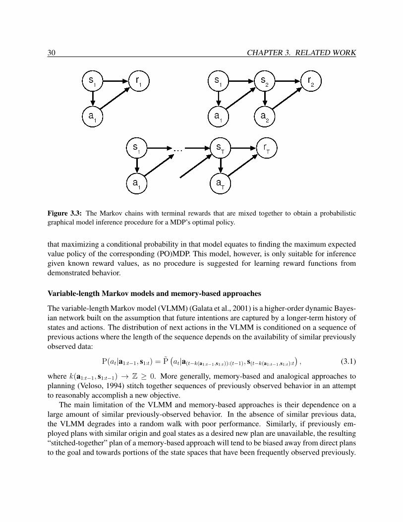
30 CHAPTER 3. RELATED WORK
Figure 3.3: The Markov chains with terminal rewards that are mixed together to obtain a probabilisticgraphical model inference procedure for a MDP’s optimal policy.
that maximizing a conditional probability in that model equates to finding the maximum expectedvalue policy of the corresponding (PO)MDP. This model, however, is only suitable for inferencegiven known reward values, as no procedure is suggested for learning reward functions fromdemonstrated behavior.
Variable-length Markov models and memory-based approaches
The variable-length Markov model (VLMM) (Galata et al., 2001) is a higher-order dynamic Bayes-ian network built on the assumption that future intentions are captured by a longer-term history ofstates and actions. The distribution of next actions in the VLMM is conditioned on a sequence ofprevious actions where the length of the sequence depends on the availability of similar previouslyobserved data:
P(at|a1:t−1, s1:t) = P(at|a(t−k(a1:t−1,s1:t)):(t−1), s(t−k(a1:t−1,s1:t):t
), (3.1)
where k(a1:t−1, s1:t−1) → Z ≥ 0. More generally, memory-based and analogical approaches toplanning (Veloso, 1994) stitch together sequences of previously observed behavior in an attemptto reasonably accomplish a new objective.
The main limitation of the VLMM and memory-based approaches is their dependence on alarge amount of similar previously-observed behavior. In the absence of similar previous data,the VLMM degrades into a random walk with poor performance. Similarly, if previously em-ployed plans with similar origin and goal states as a desired new plan are unavailable, the resulting“stitched-together” plan of a memory-based approach will tend to be biased away from direct plansto the goal and towards portions of the state spaces that have been frequently observed previously.

3.2. OPTIMAL CONTROL APPROACHES 31
3.1.2 Undirected Graphical Approaches
Undirected graphical models (Section 2.1.2), and, specifically, the conditional random field (Laf-ferty et al., 2001), have experienced remarkable success in recognition tasks for text (Lafferty et al.,2001), machine vision (Kumar & Hebert, 2006), and activities. For activity recognition tasks, sideinformation corresponds to observed characteristics (Liao et al., 2007a; Vail et al., 2007). Underthis approach, a potential function is learned for consecutive states, Yt and Yt+1, but these sequen-tial state potentials are only learned to the degree that they are needed to compensate for whenstate-observation prediction power alone is insufficient.
Ardis & Brown (2009) propose a conditional random field approach to decision inferencewhere the optimal response Y∗X to any outcome of nature, X ∼ P(X), is obtained. Toussaint(2009) arrives at a model that requires a negative reward function, but is otherwise identical, usinga directed graphical model approach where all behavior is conditioned on an additional set of vari-ables, z = 1, where P(zt|yt, xt) = e−cost(yt,xt). Ziebart et al. (2008b) propose this same distributionas an approximation to a maximum entropy formulation of modeling decision making in a Markovdecision process with stochastic dynamics. The joint distribution of responses is obtained usingthe MDP’s state transition dynamics, and nature’s outcomes are marginalized over to find the “op-timal” conditional probability when X is latent. Expanding this model to the predictive setting, wehave:
P(Yt|X1:t,Y1:t−1) ∝∑
Xt+1:T ,Yt+1:T
e−∑t cost(yt,xt) P(Xt+1:T |X1:t,Y1:t−1). (3.2)
For some simple problems with stochastic state-transition dynamics, this approach yields a policywith optimal expected reward (Ardis & Brown, 2009). However, this is only guaranteed in thespecial case of state-transition dynamics that are deterministic. We investigate the discrepancy forinference in stochastic dynamics in more detail in Section 6.3 where we provide further insightinto the underlying reason for this difference.
3.2 Optimal Control Approaches
Early control approaches to imitation learning directly model the (presumably near-optimal) policyfor future execution in similar situations. Perhaps the most successful application of this approachis ALVINN (Pomerleau, 1989), a neural network model that learns a direct mapping from camerainput to vehicle control for autonomous vehicle navigation on roadways. This approach is well-suited for predicting immediate stimulus-response behavior, like keeping a vehicle on the roadway.However, it is more difficult for predicting purposeful long-term decision making, like planning aroute between two cities. More recent approaches, including that of this thesis, attempt to learn anunderlying reward function to explain goal-directed, adaptive behavior rather than directly learningthe policy.

32 CHAPTER 3. RELATED WORK
3.2.1 Inverse Optimal ControlInverse optimal control (Boyd et al., 1994; Ng & Russell, 2000), originally posed by Kalman(1964), describes the problem of recovering an agent’s reward function, R(s,a), given a controlleror policy, when the remainder of the PRMDP,M/R, is known. We assume the PRMDP setting(Definition 2.10). Vectors of reward factors fs,a describe each available action, and the rewardfunction is assumed to be a linear function of those factors, R(s, a) = θ>fs,a parameterized byreward weights, θ. Ng & Russell (2000) formulate inverse optimal control as the recovery ofreward weights, θ, that make demonstrated behavior optimal. Unfortunately this formulation isill-posed in general.
Remark 3.1 (Ng & Russell (2000)). Demonstrated behavior may be optimal for many differentreward weights, including degeneracies (e.g., the vector of all zeros).
Ng & Russell (2000) propose a heuristic for preferring solutions that discourage deviation fromdemonstrated behavior and simple rewards (small L1 norm). However, many other heuristics canbe employed and the justification for choosing this particular heuristic is unclear. Chajewska et al.(2001) maintain a Bayesian distribution over the utility weights that are consistent with demon-strated behavior being optimal. They employ a prior that discourages degenerate weights. Anexpensive Markov chain Monte Carlo sampling procedure is required to maintain this distribution.For both of these approaches, a very serious problem still remains when modeling demonstratedbehavior.
Remark 3.2. There may be no feasible utility weight apart from degeneracies for which demon-strated behavior is optimal.
Demonstrated behavior may be inherently sub-optimal for a variety of reasons (discussed inSection 1.4) due to the fact that the Markov decision process is only an approximation of realityand decisions may be based on information that is difficult to observe or model. Allowing sub-optimality and uncertainty of behavior in the model of demonstrated behavior is needed to addressthis problem. Models based on the assumption of optimality without robustness to noisy (i.e.,sub-optimal) behavior are inappropriate as a result (Remark 3.2).
3.2.2 Feature Matching Optimal Policy MixturesAbbeel & Ng (2004) propose recovering reward weights so that a planner based on those rewardweights and the demonstrated trajectories have equal reward (in expectation) for any choice ofparameters. This formulation reduces to matching the planner and demonstrated trajectories’ ex-pected feature counts, fζ =
∑s,a∈ζ fs,a:∑
ζ
Pplanner(ζ)fζ =∑ζ
P(ζ)fζ . (3.3)

3.2. OPTIMAL CONTROL APPROACHES 33
This feature-matching constraint guarantees that the model’s expected performance will be equiv-alent to the demonstrated behavior’s realized performance for any unknown linear reward functionparameterized by θ∗, as ∑
ζ
Pplanner(ζ) (θ∗>fζ) = (θ∗>fζ). (3.4)
Abbeel & Ng (2004) employ a series of deterministic policies obtained from “solving” the optimalMDP for the distribution over trajectories. When sub-optimal behavior is demonstrated (due to theagent’s imperfection or unobserved reward factors), mixtures of those optimal policies are requiredto match feature counts:
Eplanner[f] =∑i
P(θi)
(∑ζ
P(ζ|π∗(s|θi)) fζ
). (3.5)
The proposed approach for generating a series of candidate policies is shown as Algorithm 3.1
Algorithm 3.1 Policy mixture learning algorithm
Require: State-based features f, Example MDPM, Example feature counts E[f],Ensure: A sequences of policies {π(i)}Ni=0 such that the empirical feature counts, E[f ], are
matched by a mixture of {π(i)}Ni=0 within ε.1: Randomly pick π(0) and compute E[f|π(0)].2: while for i = 1 to∞ do3: Compute t(i) = maxθ:||θ||2=1 minj∈{0..(i−1)} θ
>(E[f]−E[f|π(j)]) and let θ(i) be the parametervalues obtained by this maximum
4: if t(i) ≤ ε then5: return {π(i)}Ni=0
6: end if7: Compute optimal policy π(i) for θ(i) in MDPM8: Compute E[f|π(i)] in MDPM9: end while
The algorithm returns a series of policies that define a convex hull of expected feature countsthat contains the demonstrated feature counts. Proposed selection criteria for a single policy fromthose returned either involve expert intervention (and evaluation) or discard the performance guar-antees of the approach relative to demonstrated behavior. Alternately, a mixture of policies can beobtained from the convex hull that will match feature counts.
While this approach resolves some of the ambiguity of the original inverse optimal controlproblem (Remarks 3.1 and 3.2), it does not resolve it entirely. Many mixtures of policies that matchfeature counts can be obtained from the set of policies returned by the algorithm and from otherpolicies obtained using different randomly-chosen initial policies for the algorithm. Additionally,

34 CHAPTER 3. RELATED WORK
in the special case that only a single policy rather than a policy mixture is required to match featurecounts, there are still many choices of parameters weights that will realize that policy.
Remark 3.3. When demonstrated behavior is optimal for a single choice of reward parameters,infinitely many other choices of parameters will also make it optimal.
While Remark 3.3 is trivially true due to the invariance of the optimal policy to positivelyscaling reward parameters, it is more generally also true since a policy is optimal within somepolytope of utility parameters in the reward parameter simplex and often not for only a singlepoint.
Even ignoring these unresolved ambiguities, mixing optimal policies has undesirable propertiesfor any selection criteria. The resulting behavior obtained by first sampling parameters, θi, and thenthe optimal policy in Equation 3.5 varies drastically depending on which parameters are sampled.This can be alleviated by replacing the mixture of optimal policies with a stationary stochasticpolicy as suggested by Syed et al. (2008) (following Theorem 2.8). However, whether mixingoptimal policies or employing a corresponding stochastic policy, the model can still have verypoor predictive capabilities.
Remark 3.4. A learned policy mixture of optimal policies (or the corresponding single stochasticpolicy) can assign zero probability for demonstrated behavior if that behavior is sub-optimal forany choice of cost weights.
Figure 3.4: A simple example with three action choices where the mixture of optimal policies can have zeroprobability for demonstrated behavior if path 2 is demonstrated.
Consider the simplified example in Figure 3.4 with three action choices corresponding to Paths1, 2, and 3, and one feature characterizing each action choice. For sake of argument, assume thatdemonstrated behavior consists solely of selecting path 2. There are only two non-degenerate op-timal policies: for π1, θ < 0 implies path 1 should be selected, and for π2, θ2 > 0 implies path 3should be selected1. These can be appropriately mixed with α1 = 0.4 and α2 = 0.6 so that demon-strated feature counts and the feature counts expected under the optimal policy mixture match,however note that there is zero probability of the demonstrated action (path 2) in this solution.
1For parameters θ = 0, ties are typically broken according to an arbitrarily chosen secondary tie-breaking criteria.For example, if the order of consideration were employed, Path 1 would be selected for θ = 0.

3.2. OPTIMAL CONTROL APPROACHES 35
3.2.3 Maximum Margin PlanningRatliff et al. (2006) resolve the ambiguity of choosing a single set of parameter weights to makedemonstrated behavior optimal (Remark 3.3) by posing inverse optimal control as a maximummargin problem. They reduce a quadratic program for solving this problem into the followingconvex objective:
Cq(θ) =1
n
n∑i=1
βi
(maxµ∈Gi
(θ>Fi + l>i
)µ− θ>Fiµi
)q+λ
2||θ||2, (3.6)
where µ are expected state visitation counts constrained by the MDP’s structure (G), µi are theempirical visitation counts for example i, and li is an augmented state loss, li : S → R, thatassigns higher loss to states visited in example i.
Algorithm 3.2 Maximum margin planning
Require: State-based features f, Example MDPs {Mi}, Example feature counts {E[f]i}, Exampleloss augmentation {li}, Learning rate r, Regularization parameter C, Iterations T
Ensure: Parameters, θ, that (approximately) optimize the maximum margin objective.1: θ ← 02: for t = 1 to T do3: Compute optimal π∗(s) for each loss-augmented cost map θ>fi + l>i in MDPMi
4: Compute E[f|π∗(s)]i in MDPMi
5: Compute sub-gradient g = θ + C(∑
i(E[f|π∗(s)]i − E[f]i))6: θ ← θ − r
tg
7: end for8: return θ
The sub-gradient algorithm (Algorithm 3.2) for optimizing the maximum margin planning ob-jective (Equation 3.6) operates by effectively lowering the costs of actions that are away from thedemonstrated trajectory and finding cost weights making the cost-augmented demonstrated trajec-tory optimal. While the approach yields a unique solution, it suffers from significant drawbackswhen no single reward function makes demonstrated behavior both optimal and significantly betterthan any alternate behavior. This arises quite frequently when, for instance, the behavior demon-strated by the agent is imperfect, or the planning algorithm only captures a part of the relevantstate-space and cannot perfectly describe the observed behavior.
A feature boosting approach (Ratliff et al., 2007) partially addresses this sub-optimal behaviorproblem by creating a larger (non-linear) class of features to explain demonstrated behavior asoptimal. While this may succeed, it also runs the risk of crafting features that overfit to the trainingdata. The methods presented in this thesis differ from maximum margin planning in the explicittreatment of uncertainty under the maximum causal entropy approach. This uncertainty is neededto address suboptimal behavior.

36 CHAPTER 3. RELATED WORK
3.2.4 Game-Theoretic CriteriaSyed & Schapire (2007) employ a game-theoretic approach that maximizes performance relativeto the demonstrated behavior for the worst-case choice of reward function. When backgroundknowledge is available indicating the sign of the different cost factors (i.e., whether each featureis “good” and should be maximized or “bad” and should be minimized), the learned model canoutperform demonstrated behavior.
Remark 3.5 (Syed & Schapire (2007)). When it is assumed that ∀i θi ≥ 0, then if ∀i EP [fi] ≥EP[fi], the distribution P has expected reward guaranteed to be higher than the reward of demon-strated behavior on the unknown cost function θ∗.
This approach similarly yields a mixture of policies, which is later converted to a stationarypolicy using Theorem 2.8 and learned using a linear programming formulation (Syed et al., 2008).It also suffers from potentially assigning zero probability to demonstrated behavior.
3.2.5 Boltzmann Optimal-Action-Value DistributionAn alternative to mixing optimal policies to obtain a non-deterministic behavior model is to directlyobtain a distribution as a function of the MDP’s optimal action values, Qθ(s, a)∗, obtained by firstsolving the Bellman equation (Theorem 2.7). A natural approach to regressing from a set of realvalues to a probability distribution is the Boltzmann probability distribution. Inference underthis model was first proposed for goal inference (Baker et al., 2006, 2007) using the true costs ofgenerated behavior in synthetic experiments:
P(action a|state s) =eβQθ(s,a)∑
action a′ eβQθ(s,a′)
. (3.7)
The scale parameter, β, determines the stochasticity of the policy. As β →∞, the policy becomesdeterministic2. When Qθ(s, a) is learned from data, its scale is also learned and β is superfluous.
Two approaches for learning parameters in this model have been proposed. Neu & Szepesvari(2007) employ this distribution within a loss function penalizing the squared difference in proba-bility between the model’s action distribution and the demonstrated action distribution. Ramachan-dran & Amir (2007) utilize it within a Bayesian approach to obtain a posterior distribution overreward values using Markov Chain Monte Carlo simulation. The main weaknesses of the modelare summarized by Remark 3.6 and Remark 3.7.
Remark 3.6 (Neu & Szepesvari (2007)). The likelihood of data in the Boltzmann optimal-action-value distribution is not convex in its parameters θ.
2This assumes that no two actions have equivalent reward. If there are multiple optimal actions, they will haveequal probability.

3.2. OPTIMAL CONTROL APPROACHES 37
The non-convexity of the data likelihood function under the Boltzmann model (Remark 3.6)makes finding optimal model parameters difficult, and non-convex distributions such as this are asa result generally less preferred than convex models for computational efficiency reasons.
Remark 3.7. The relationship between a policy’s expected reward and its probability in the Boltz-mann optimal-action-value distribution is not monotonic.
Additionally, the non-monotonic relationship between a policy’s expected reward and its prob-ability within the model (Remark 3.7) has a few undesirable consequences: the most likely policywithin the model does not necessarily have the highest probability within the model and policieswith equal reward do not necessarily have equal probability (and vice versa). Also, this modelprovides no guarantees of performance relative to the demonstrated behavior.
3.2.6 Robust and Approximate Optimal ControlAnother branch of research makes optimal decisions based on the Kullback-Leibler divergence ofdecision setting dynamics to realize robust control techniques (Bagnell, 2004; Nilim & El Ghaoui,2005). Specifically, this technique provides strong PAC-style performance guarantees when thetransition dynamics of a decision setting are only approximately known. It was recently observedthat the resulting probabilistic model is a linearization of the Bellman equations (Kappen, 2005;Todorov, 2006). This linearized view enables more efficient techniques for approximating theoptimal policy’s value by solving a system of linear equations. The problem is formulated as acontinuous control problem where the action cost is defined as the Kullback-Liebler divergence ofthe employed action’s implied dynamics and a set of “passive” dynamics, P0(sj|si). The actions inthis approach directly determine the next state—there are no stochastic dynamics given the action,but a high cost is paid to employ a deterministic policy that differs from the passive dynamics. Theoptimal action under this formulation yields stochastic dynamics:
P ∗KL(sj|si) =P0(sj|si) ev
∗KL(sj)∑
skP0(sk|si) ev
∗KL(sk)
. (3.8)
In general, state transitions in Markov decision processes are dependent on the action and eachaction does not deterministically lead to a different next state. Todorov proposes a method forembedding general Markov decision processes within this framework (2009b), but this approachis approximate and only anecdotal evidence has been provided to demonstrate its validity.
The compositionality of control laws within the linear Bellman approach is described by Todorov(2009a) and employed (approximately) for generating realistic character animation (da Silva et al.,2009).
Remark 3.8 (following Todorov (2009a)). Let π(1)KL and π(2)
KL be optimal KL policies for terminalreward V (1)
final(s) and V (2)final(s) in a first-exit linear Bellman model with corresponding path integrals

38 CHAPTER 3. RELATED WORK
ZV (1)(s) and ZV (2)(s). Then for α ∈ [0, 1], βπ(1)KL + (1−β)π
(2)KL is an optimal linear Bellman policy
for terminal reward αV (1)final(s) + (1− α)V
(2)final(s), where β =
αzV (1) (s)
αZV (1) (s)+(1−α)Z
V (2) (s).
Our work generalizes this idea of efficient composability to a full Bayesian treatment of latentgoal states (Ziebart et al., 2008c) in Chapter 11. Specifically, it not only incorporates arbitrary ter-minal rewards, but also addresses appropriately updating those rewards based on observed behav-ior when the goal of the behavior is unknown. We apply this approach to vehicle route preferenceprediction in Chapter 12 and pedestrian trajectory prediction in Chapter 13.
A learning approach under the linear Bellman equation perspective (Krishnamurthy & Todorov,2010) is identical to the maximum causal entropy model of this thesis for deterministic dynamics(Ziebart et al., 2008b), except that a value function rather than a (feature-based) cost function islearned3. Value function learning can be viewed as a special case of cost function learning whereeach state has its own unique feature. The advantage of learning the value function is the simplicityof not having to solve a forward inference problem. For some domains, that forward inferenceproblem can be prohibitively expensive. However, there is also a large disadvantage because theresulting model is then unable to generalize. For example, changes in end-state constraint (i.e.,goal), state transition dynamics, or transfer to similarly-parameterized MDPs require a learnedcost function rather than a learned value function. Krishnamurthy & Todorov (2010) propose alinear regression approach to obtain a parametric cost function from the learned values, howeverthis approach provides no predictive guarantees and is not evaluated in that work. A method ofgeneralizing by estimating the value function as a mixture of Gaussians is proposed to reducedependence on training data for accurate estimation, but this still does not transfer to other goalsor settings.
We investigate some of the restrictions of linearizing the Bellman equation relative to the prin-ciple of maximum causal entropy approach developed in this thesis in Section 6.3 and relate thecompositionality of optimal control in the linearized Bellman equation approach to our techniquesfor efficient Bayesian inference of latent goals in Chapter 11.
3.2.7 Noise-Augmented Optimal Actions
A final, and quite general approach from the optimal control perspective for making an optimalpolicy stochastic is to augment the optimal value function with a sampled noise distribution, εs,a,and generate a stochastic policy using many sampled deterministic policies:
π(s) = argmaxa
Q∗(s, a) + εs,a. (3.9)
3The claimed “passive dynamics” generalization is equivalent to optimizing the relative entropy and is generalizedvia Remark 5.3 by simply adding corresponding action features.

3.3. DISCRETE CHOICE THEORY 39
Any distribution can be employed for the error term, however the generality comes at a cost:simulation is required rather than closed-form analysis. Nielsen & Jensen (2004) take this ap-proach to model decisions in an influence diagram and to then learn the underlying utility functionupon which Q∗(s, a) is based using Markov chain Monte Carlo sampling strategies. In this thesis,we employ basic principles to obtain a theoretically-justified error term. This provides predic-tive guarantees and computational efficiency benefits that the noise-augmented approach generallylacks.
3.3 Discrete Choice TheoryEconomists have long studied models for estimating the probability of different choice selectionsfrom a set of discrete options under various axiomatic formulations and noise assumptions. Wereview some of the approaches established from that perspective here.
3.3.1 Multinomial and Conditional LogitChoice models estimate the probability that an individual with characteristics defined by vectorxi will select one of c ∈ C choices (i.e., P(y = c|x, C)). Luce (1959) derived an axiomaticprobabilistic model based on the independence of irrelevant alternatives (IIA) axiom. Under theIIA axiom, the relative odds between two choices are unaffected by the addition of options to theset of choices.
∀c1,c2∈Ca,CbP(y = c1|x, Ca)P(y = c2|x, Cb)
=P(y = c1|x, Ca)P(y = c2|x, Cb)
(3.10)
The resulting multinomial logit probabilistic model has the following form:
P(y = c|x, Ca, θ) =eθ>c x∑
c′∈C eθ>c′x, (3.11)
which is a log-linear (logistic regression) model.McFadden (1974) proposes employing characteristics of the available options, zc, within a
model based on the IIA axiom. When both characteristics of the individual and the options areemployed, the probability distribution of this conditional logit model takes the following form:
P(y = c|x, z, C, θ, φ) =eθ>c x+φ>zc∑
c′∈C eθ>c′x+φ>zc′
, (3.12)
which is similarly a log-linear model. This approach has the advantage of providing specification tothe predictive probability distribution based on the characteristics of the different available options.

40 CHAPTER 3. RELATED WORK
3.3.2 Criticisms of the Independence of Irrelevant Alternatives AxiomA common criticism of the IIA axiom (and the multinomial and conditional logit models that em-ploy it) is its inability to take into account (near) perfect substitutes. Consider the “Red Bus/BlueBus” example (McFadden, 1974), where the options of driving a car or taking a red bus are avail-able to a commuter with equal probability under the model. If a blue bus option is added, andcommuters are indifferent to bus color, one would expect a probability of 50%, 25%, and 25% forcar, red bus, and blue bus, but instead each is equally probable under the IIA axiom.
A number of alternate discrete choice models have been proposed that relax the IIA axiom toaddress this scenario.
3.3.3 Nested LogitThe nested logit discrete choice model (Ben-Akiva, 1974) incorporates correlation among similargroups of disjoint choices (nests), C1, C2, ... such that C = ∪k Ck and ∀j 6=k Cj ∩ Ck = Ø. Theprobability of a choice i in clique Ck is specified by the chain rule:
P(i) = P(Ck) P(i|Ck), (3.13)
with probabilities defined by:
P(Ck) =eZCk+λ ln
∑i∈Ck
eVi∑nj=1 e
ZCj+λ ln∑i∈Cj
eViand (3.14)
P(i|Ck) =eVCi∑j∈Ck e
VCj.
The λ ∈ [0, 1] parameter in this model is related to the correlation between choices within eachof the nests. When λ = 1, this model reduces to a standard logit model.
3.4 DiscussionWe now discuss the relations of the reviewed approaches to each other and to the maximum causalentropy approach contributed by this thesis.
3.4.1 Connections Between ApproachesDespite being developed under varying perspectives with differing assumptions and for differentpurposes, there are a number of similarities between these approaches. The linear Bellman opti-mal control model (Todorov, 2006) and the conditional multinomial logit discrete choice model

3.4. DISCUSSION 41
(McFadden, 1974) are both exponential family models that can be equivalently expressed as a spe-cial form of conditional random fields with potentials that correspond to rewards (Ardis & Brown,2009; Toussaint, 2009). Evaluating the robust MDP model by the power method is equivalent toforward or backward algorithms for chain conditional random field inference and is a special caseof the nested logit model’s hierarchical inference procedure (Equation 3.14).
The independence of irrelevant alternatives axiom of discrete choice theory also has analogiesin the optimal control approaches for decision modeling. Specifically, the correlation-based pa-rameter of the nested logit model has a number of parallels. The Boltzmann optimal-action-valuedistribution does not obey the IIA axiom and is similar to the λ = 0 nested logit model. Moregenerally, the discount factor, which is commonly employed to make the Bellman equations forinfinite time horizons convergent, when applied within the linear Bellman optimal control modelis very similar to the effect that λ has in the nested logit model.
3.4.2 Relation to Thesis ContributionsInformation revelation settings
The primary contribution of this thesis is a principled approach for modeling the conditional prob-abilities of variables in settings with side information that is revealed over time from a knownconditional probability distribution. Markov decision processes with stochastic dynamics matchthis information revelation setting because the next state is random and only revealed after an ac-tion is made. Conditional random fields are ill-suited for this setting because they are based onthe principle of maximum conditional entropy, which assumes full knowledge of random side in-formation in advance. As a consequence, there is a disconnect between maximizing conditionallikelihoods in a conditional random field and maximizing the expected reward in a correspondingMDP (Remark 6.17). Similarly, the linear Bellman equation model relies on an imprecise em-bedding to model general MDPs because linearization alone is inappropriate for dealing with theinformation availability of the general MDP.
The maximum causal entropy approach of this thesis provides a means for probabilisticallymodeling behavior within settings characterized by sequentially revealed side information (e.g.,such as the sequence of states in a Markov decision process) so that maximum likelihood policyestimation is equivalent to expected reward maximization. This is in contrast to the Boltzmannoptimal value action model, where the maximum likelihood policy and the maximum expectedreward policy within the Markov decision process do not necessarily match. An additional advan-tage of the maximum causal entropy approach is that the optimization for learning parameters inthe model is convex.
Cost potential function learning
In the special case that the corresponding Markov decision process has deterministic state-transitiondynamics, revealing the next state provides no new information. This is due to the fact that the next

42 CHAPTER 3. RELATED WORK
state is already known from the choice of action and current state. In this setting, the principle ofmaximum causal entropy reduces to a probabilistic model that matches the linear Bellman model(Todorov, 2006), conditional random field (Ardis & Brown, 2009; Toussaint, 2009), and condi-tional logit (McFadden, 1974) models of behavior.
While the development of the linear Bellman model (Todorov, 2006) precedes the maximumentropy approach for decision modeling (Ziebart et al., 2008b), its purpose was for efficient ap-proximate inference of the optimal policy and optimal value function. More recent attempts toapply the linear Bellman model for learning (Krishnamurthy & Todorov, 2010) propose learningvalue functions rather than the cost functions learned in the maximum entropy approach. As pre-viously discussed, the computational benefits of the approach come at the cost of not being able togeneralizes to changes in the problem setting.
Similarly, the conditional random field model of Markov decision processes has only beenpreviously applied for purposes of inference based on known reward values (Ardis & Brown, 2009;Toussaint, 2009). We note that our work (Ziebart et al., 2008b) represents the first employment ofthis model for the purpose of learning from observed behavior. Additionally, the use of featuresassociated with “states” rather than observations is atypical from the standard CRF perspective.The principle of maximum causal entropy generalizes the validity of this approach to settings withstochastic state dynamics.
The conditional logit model is perhaps the most similar to the maximum entropy model ofdecision making on decision tasks with no information revelation. It is important to note the limitsof the conditional logit approach in its previous applications. For route preference modeling, forinstance, the first step of applying logit models when given a road network with infinite possiblepaths between two points is to employ a route selection algorithm that generates a tractable subsetof paths to consider. We view our approach as an extension of the efficiency of the conditional logitmodel from trees of decisions to graphs with (potentially) infinite sequences of choices. Maximumcausal entropy also generalizes the discrete choice models to settings with stochastic state transitiondynamics.

Part II
Theory
43

44
Overview of Part IIPart II of the thesis provides the formulations and theoretical properties of the maximum causalentropy approach needed for modeling sequences of behavior, as well as the justifications for itsuse as a predictive tool.
Chapter 4 reviews the theory of causal information. This less widely known extension ofinformation theory enables its applicability to settings with feedback and interaction.
Chapter 5 presents the general formulation for modeling a sequence of variables that is causallyconditioned on a sequence of additional sequentially-revealed variables. Two types of constraintsare introduced: affine equality constraints and convex inequality constraints, which generally cor-respond to efficiency and rationality requirements in this thesis.
Chapter 6 applies the general maximum causal entropy formulation to the inverse optimal con-trol setting of finding the reward, utility, or cost function of the parametric Markov decision pro-cess or linear-quadratic regulator frameworks introduced in Chapter 2. Equality constraints areemployed to match statistical expectations of characteristics of demonstrated behavior. Inferenceunder this model corresponds to a softened application of the Bellman equation, leading to a num-ber of simple inference algorithms in Part III.
Chapter 7 extends the maximum causal entropy approach to the influence diagram framework(Chapter 2). Whereas in the inverse optimal control setting of Chapter 6, only future side informa-tion is unknown or latent at each point in time, the formulation of this chapter allows current andpast information to also be unknown. This corresponds to common decision settings with partialinformation, such as the POMDP, and to collaborative multi-agent coordination. We establish animportant boundary on the applicability of the maximum causal entropy approach: perfect recallof past decisions is required for many of the theoretical niceties introduced in Chapter 5 to hold.
Chapter 8 demonstrates the wider applicability of the maximum causal entropy approach byapplying it to multi-agent game play. The inequality constraints of Chapter 5 are employed toenforce rationality requirements of players’ strategies in sequential games. This enables a novel,well-specified correlated equilibrium solution concept with log-loss prediction guarantees in thesequential setting of Markov games.
Together, the theoretical developments of these five chapters provide a broad scope of ap-plicability for the maximum causal entropy approach for predicting behavior under a number ofbehavior frameworks.

Chapter 4
The Theory of Causal Information
“Nobody knows what entropy really is, so in a debate you will always have the advantage.”– John von Neumann (Mathematician, 1903–1957)
The field of information theory was developed primarily by Shannon’s seminal communica-tions work (1948). It enables the quantification of the amount of information provided by randomvariables. Information measures for joint, conditional, marginal, and relative distributions are wellknown. They are frequently employed in communication, control, and machine learning appli-cations. In this chapter, we review those measures and their properties. We then review the lesswidely known causal extension of information theory. This extension enables the applicabilityof information theory in settings of interaction and feedback. It serves as the backbone of ourapproach for creating predictive distributions for human behavior in those settings.
4.1 Information TheoryWe provide a brief overview of information-theoretic measures. We refer the reader to Cover &Thomas (2006)’s excellent book on the topic for a more thorough coverage of information theoryand its applications.
4.1.1 Entropy and InformationShannon’s information entropy of distribution P over random variable X measures the uncer-tainty of that probability distribution.
Definition 4.1. The entropy of a discrete random variable, X, distributed according to P is:
HP(X) = EP(X)[− log P(x)]
= −∑x∈X
P(x) log P(x). (4.1)
45

46 CHAPTER 4. THE THEORY OF CAUSAL INFORMATION
For continuous-valued variables1, the entropy is:
HP(X) =
∫x
P(x) log P(x) dx. (4.2)
When log2 is used, the discrete entropy (4.1) measures the average number of bits needed for abinary message that encodes a sample from distribution P. A uniform distribution maximizes thisentropy measure, while an entropy of zero corresponds to a single point distribution.
When X is a vector of variables, X1:T , rather than a scalar, the joint entropy measures theuncertainty of the joint distribution, P (X1:T ).
Definition 4.2. The joint entropy of the vector of random variables, X1:T , distributed according toP(X1:T ) is:
HP(X1:T ) = EP(X1:T )[− log P(x1:T )]
= −∑x1:T
P(x1:T ) log P(x1:T ). (4.3)
The cross entropy measures the amount of uncertainty of the distribution P under a differentdistribution Q both over random variable X .
Definition 4.3. The cross entropy of distribution P under distribution Q is:
H(P, Q) = EP(X)[− logQ(x)]
= −∑x∈X
P(x) logQ(x). (4.4)
From the coding perspective, the cross entropy is the expected number of bits needed to encodesamples from P under the incorrect probability distribution, Q. It is equivalent to the log-loss ofdistribution Q evaluated by predicting data actually distributed according to P .
The conditional entropy extends information theory to conditional probability distributionsettings. It measures the average amount of information needed to recover Y given that X isknown.
Definition 4.4. The conditional entropy of Y given X distributed according to P(Y |X) is:
HP(Y |X) = EP(X,Y )[− log P(y|x))]
= −∑y∈Y
∑x∈X
P(y, x) log P(y|x), (4.5)
for scalar random variables Y and X and naturally extends to vectors of random variables.1We will typically only consider the discrete-valued expansion in this chapter. The continuous-valued analog can
be obtained from the continuous-valued definition of expectations.

4.1. INFORMATION THEORY 47
The entropy of the previously described distributions are implicitly relative to a uniform distri-bution. In general, other relative distributions can be employed. The relative entropy measures theadditional amount of information needed to code samples of P according to a different encodingdistribution, Q.
Definition 4.5. The relative entropy of distribution P relative to distribution Q is:
H(P //Q) = EP(X)
[log
P(x)
Q(x)
]=∑x∈X
P(x) logP(x)
Q(x). (4.6)
We employ this modified notation to avoid conflict with causal entropy measure notation2.
The relative entropy is more commonly known as the Kullback Leibler-divergence (Kullback &Leibler, 1951) between P and Q: DKL(P ||Q) , H(P //Q).
Definition 4.6. The mutual information of two variables distributed according to P(Y,X) is:
I(X;Y ) = EP(X,Y )
[log
(P(x, y)
P(x) P(y)
)]=∑x∈X
∑y∈Y
P(x, y) log
(P(x, y)
P(x) P(y)
).
The mutual information (Definition 4.6) provides the amount of information shared by tworandom variables.
Definition 4.7. The conditional mutual information of two variables conditionally distributed(given an additional variable) according to P(Y,X|Z) is:
I(X;Y |Z) = EP (X,Y,Z)
[log
(P(x, y|z)
P(x|z) P(y|z)
)]=∑z∈Z
P (z)∑x∈X
∑y∈Y
P (x, y|z) log
(P(x, y|z)
P(x|z) P(y|z)
)
Lastly, the conditional mutual information (Definition 4.7) provides the amount of informa-tion shared by two random variables conditioned on a third variable.
2Typically the relative entropy is denoted asH(P ||Q). However, this conflicts with the existing notation employedfor the causal entropy we will employ later. Hence, we employ the alternate notation
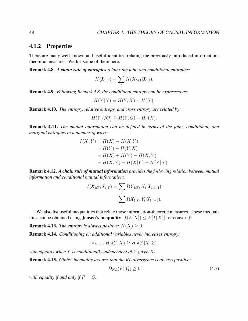
48 CHAPTER 4. THE THEORY OF CAUSAL INFORMATION
4.1.2 PropertiesThere are many well-known and useful identities relating the previously introduced information-theoretic measures. We list some of them here.
Remark 4.8. A chain rule of entropies relates the joint and conditional entropies:
H(X1:T ) =∑t
H(Xt+1|X1:t).
Remark 4.9. Following Remark 4.8, the conditional entropy can be expressed as:
H(Y |X) = H(Y,X)−H(X).
Remark 4.10. The entropy, relative entropy, and cross entropy are related by:
H(P //Q) , H(P, Q)−HP(X).
Remark 4.11. The mutual information can be defined in terms of the joint, conditional, andmarginal entropies in a number of ways:
I(X;Y ) = H(X)−H(X|Y )
= H(Y )−H(Y |X)
= H(X) +H(Y )−H(X, Y )
= H(X, Y )−H(X|Y )−H(Y |X).
Remark 4.12. A chain rule of mutual information provides the following relation between mutualinformation and conditional mutual information:
I(X1:T ; Y1:T ) =∑t
I(Y1:T ;Xt|X1:t−1)
=∑t
I(X1:T ;Yt|Y1:t−1).
We also list useful inequalities that relate those information-theoretic measures. These inequal-ities can be obtained using Jensen’s inequality: f(E[X]) ≤ E[f(X)] for convex f .
Remark 4.13. The entropy is always positive: H(X) ≥ 0.
Remark 4.14. Conditioning on additional variables never increases entropy:
∀X,Y,Z HP(Y |X) ≥ HP(Y |X,Z)
with equality when Y is conditionally independent of Z given X .
Remark 4.15. Gibbs’ inequality assures that the KL divergence is always positive:
DKL(P ||Q) ≥ 0 (4.7)
with equality if and only if P = Q.

4.1. INFORMATION THEORY 49
4.1.3 Information Theory and GamblingInformation theory and gambling have many close connections. We summarize the main resultsof Cover & Thomas (2006) in this section to illustrate those connections. Many perspectives ongambling have focused on maximizing the expected payoff of a (set of) bet(s). This strategy hasthe unfortunate problem that over a large enough time span, the realized payoff by employingan expected utility maximizing strategy will be zero with high probability. This is known as thegambler’s paradox. An alternate perspective is to maximize the rate of growth of investment.
More concretely, Cover & Thomas (2006) consider an m horse race where the payoff on abet is bioi, where bi is the fraction of total wealth bet that horse i will win, and oi is the payoffmultiplier if horse i does win. It is assumed that the initial wealth of the gambler is 1, and all ofthe gambler’s wealth is bet during each race. After a sequence of races, the gambler’s wealth willbe:
Sn =n∏t=1
S(Yt), (4.8)
where S(Y ) = b(Y ) o(Y ) and Yt is the winning horse. The expected doubling rate of invest-ment is then: W (b, p) = E[logS(Y )] =
∑mk=1 pk log(bkok) when the winning horse is distributed
according to p.
Theorem 4.16 (from Cover & Thomas (2006)). Proportional gambling, b∗ = p, is log-optimalwith optimal doubling rate:
W ∗(p) =k∑i=1
pi log oi −H(p). (4.9)
Theorem 4.17 (from Cover & Thomas (2006)). When side information, Xt, is provided beforeeach race, the optimal doubling rate,
W ∗(Y|X) =k∑i=1
P(y|x) log oi −H(Y|X), (4.10)
is obtained by b∗ = p(y|x). The difference in growth rate by having the side information is themutual information between the side information and the winning horse variables:
∆W = W ∗(Y|X)−W ∗(Y) = I(Y; X). (4.11)
Thus, there are very strong connections between information-theoretic measures and invest-ment growth rates in gambling. The causal information investigated in this thesis expand this gam-bling perspective to settings where the outcomes of consecutive horse races are dependent, and thethe revealed side information is also dependent on previous side information and race outcomes.

50 CHAPTER 4. THE THEORY OF CAUSAL INFORMATION
4.2 Causal Information
4.2.1 Sequential Information Revelation and Causal Influence
Many important problem settings with sequential data involve partial information, feedback, andinteraction. For example, in decision settings with stochastic dynamics, future side information(i.e., the future state), X, is unknown during earlier points of interaction (Figure 4.1). As a con-sequence, the future side information should have no causal influence in our statistical models ofinteraction until after it is revealed. In other words, the specific instantiation value, xt2 , should haveno causal influence on yt1 for t1 < t2. However, this does not imply a statistical independence—theinfluence of earlier interactions on future side information should not be ignored. In the case ofstochastic dynamics, the actions chosen do influence the future state.
Figure 4.1: The sequence of side information variables, X, and conditioned variables, Y, that are revealedand selected over time.
More formally this notion of causal influence means that if a future side information variablewere secretly fixed to some value by intervention (Pearl, 2000) rather than generated accordingto its conditional probability distribution, the distribution over all earlier variables would be unaf-fected by this change. In contrast, if by intervention some side information variable were fixed tosome value, the value of variables does influence future conditioned variables.
4.2.2 Causally Conditioned Probability
The causally conditioned probability (Kramer, 1998) from the Marko-Massey theory of directedinformation (Marko, 1973; Massey, 1990) is a natural extension of the conditional probability,P(Y|X), to the situation where each Yt (for t = 1..T ) is conditioned on only a portion of the Xvariables, X1:t, rather than the entirety, X1:T .
Definition 4.18. Following the previously developed notation (Kramer, 1998), the probability of Y

4.2. CAUSAL INFORMATION 51
causally conditioned on X is:
P(YT ||XT ) ,T∏t=1
P(Yt|X1:t,Y1:t−1). (4.12)
We will often consider Y to be actions or controls applied to a system and X to be the system’sstate in this thesis. This interpretation can be useful in understanding the approach, but it is im-portant to note that Y and X can represent any sequentially revealed information where the causalassumption that future side information does not influence earlier variables is reasonable.
Figure 4.2: A sequence of variables, Y1:T conditioned (left) and causally conditioned (right) on a corre-sponding sequence of side information variables, X1:T . In the conditional setting, edges cannot be directedupwards from X variables to Y, and typically the distribution over X is not modeled at all. In the causallyconditioned setting, edges cannot be directed leftward from future time step variables, Xt+1:T ,Yt+1:T toprevious time step variables, X1:t,Y1:t.
The subtle, but significant difference between the causally conditioned distribution and theconditional probability distribution, P(Y|X) =
∏Tt=1 P(Yt|X1:T ,Y1:t−1)—where each Yt variable
is conditioned on all X variables—is illustrated by Figure 4.2. In the conditional distribution,many edges are directed against the direction of time from Figure 4.1. This distinction serves asthe underlying basis for the maximum causal entropy approach.
4.2.3 Causal Entropy and InformationInformation-theoretic measures based on the standard conditional probability distribution also ex-tend to the causally conditioned probability distribution (Equation 4.12).
Definition 4.19. The causal entropy (Kramer, 1998; Permuter et al., 2008) of Y given X is:
H(YT ||XT ) , EY,X[− log P(YT ||XT )] (4.13)
=T∑t=1
H(Yt|X1:t,Y1:t−1).

52 CHAPTER 4. THE THEORY OF CAUSAL INFORMATION
The causal entropy (Definition 4.19) measures the uncertainty present in the causally condi-tioned distribution of the Y variable sequence given the preceding partial X variable sequence. Itcan be interpreted as the expected number of bits needed to encode the sequence Y1:t given theprevious Y variables and sequentially revealed side information, X1:t, which has been revealed ateach point in time and excluding unrevealed future side information, Xt+1:T .
The causal information (also known as the directed information) is a measure of the sharedinformation between sequences of variables when the variables are revealed sequentially.
Definition 4.20. The causal information (or directed information) of two vectors of variables is:
I(XT → YT ) =∑t
I(X1:t;Yt|Y1:t−1)
It differs from the chain rule for mutual information (Remark 4.12) in that the X variable vector islimited to t rather than T on the right-hand side.
4.2.4 PropertiesUsing the causally conditioned probability distributions, any joint distribution can be expressedvia the chain rule3 as P(Y,X) = P(YT ||XT ) P(XT ||YT−1). Our approach estimates P(YT ||XT )based on a provided (explicitly or implicitly) distribution of the side information, P(XT ||YT−1) =∏
t P(Xt|X1:t−1,Y1:t−1). By employing this relationship between the joint and causal distributions,Equation 4.13 can be equivalently expressed in terms of the joint-relative entropy.
Remark 4.21. The causally conditioned entropy is related to the joint and relative entropy as:
H(YT ||XT ) = H(Y,X)−H(XT ||YT−1) (4.14)= const.−H (Y,X//P0(X,Y))
Equation 4.14 is the joint distribution over X and Y relative to a baseline joint distribution,P0(X,Y), that obeys the provided side information distribution, P(XT ||YT−1), and is otherwiseuniform over P(YT ||XT ). We employ the “//” notation introduced in Definition 4.5 to representthe relative entropy and distinguish it from our employed causal entropy notation, “||.”
It is easy to verify that the causal entropy upper bounds the conditional entropy; intuitively thisreflects the fact that conditioning on information from the future (i.e., acausally) can only decreaseuncertainty.
Theorem 4.22. Generally, the conditional and causal entropies are related as:
H(Y|X) ≤ H(YT ||XT ) ≤ H(Y) ≤ H(Y,X), (4.15)
3More generally, other decompositions of the form: P(Y,X) = P(YT ||XT−∆1) P(XT ||YT−∆2) for 0 ≤ ∆1 <∆2 are possible, including the “standard” conditional decomposition, P (Y,X) = P (X)P (Y|X).
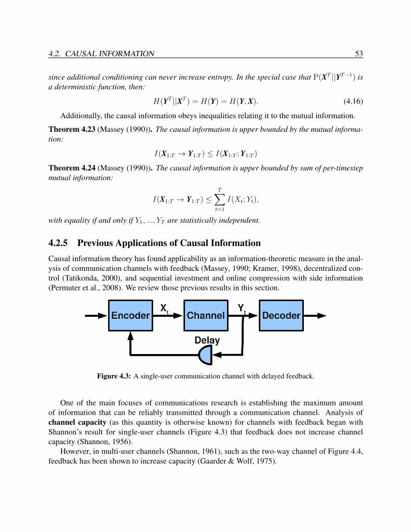
4.2. CAUSAL INFORMATION 53
since additional conditioning can never increase entropy. In the special case that P(XT ||YT−1) isa deterministic function, then:
H(YT ||XT ) = H(Y) = H(Y,X). (4.16)
Additionally, the causal information obeys inequalities relating it to the mutual information.
Theorem 4.23 (Massey (1990)). The causal information is upper bounded by the mutual informa-tion:
I(X1:T → Y1:T ) ≤ I(X1:T ; Y1:T )
Theorem 4.24 (Massey (1990)). The causal information is upper bounded by sum of per-timestepmutual information:
I(X1:T → Y1:T ) ≤T∑t=1
I(Xt;Yt),
with equality if and only if Y1, ..., YT are statistically independent.
4.2.5 Previous Applications of Causal InformationCausal information theory has found applicability as an information-theoretic measure in the anal-ysis of communication channels with feedback (Massey, 1990; Kramer, 1998), decentralized con-trol (Tatikonda, 2000), and sequential investment and online compression with side information(Permuter et al., 2008). We review those previous results in this section.
Figure 4.3: A single-user communication channel with delayed feedback.
One of the main focuses of communications research is establishing the maximum amountof information that can be reliably transmitted through a communication channel. Analysis ofchannel capacity (as this quantity is otherwise known) for channels with feedback began withShannon’s result for single-user channels (Figure 4.3) that feedback does not increase channelcapacity (Shannon, 1956).
However, in multi-user channels (Shannon, 1961), such as the two-way channel of Figure 4.4,feedback has been shown to increase capacity (Gaarder & Wolf, 1975).

54 CHAPTER 4. THE THEORY OF CAUSAL INFORMATION
Figure 4.4: A two-way communication channel with delayed feedback.
Theorem 4.25 (Massey (1990)). If X1:T and Y1:T are input and output sequences of a discretechannel, and U1:K is a source output sequence (i.e., message to transmit), then:
I(U1:K ; Y1:T ) ≤ I(X1:T → Y1:T )
Combining Theorem 4.23 with Theorem 4.25, Massey (1990) establish the causal informationas a tighter bound on the mutual information between the source message and the discrete channeloutput in communication channels with feedback.
Theorem 4.26 (Corollary 4.1 of Kramer (1998)). The capacity region CTWC of the discrete mem-oryless common-output two-way channel is the closure of the set of rate-pairs (R1, R2) such that:
R1 = I(X1,1:T → Y1:T ||X2,1:T )
R2 = I(X2,1:T → Y1:T ||X1,1:T )
where T is a positive integer and where:
P(X1,t, X2,t|X1,1:t−1,X2,1:t−1,Y1:t−1) = P(X1,t|X1,1:t−1,Y1:t−1) P(X2,t|X2,1:t−1,Y1:t−1)
for all t = 1, 2, ..., T .
With Theorem 4.26, Kramer (1998) proves the relationship between directed information andchannel capacity in the memory-less common-output two-way channel setting.
Tatikonda (2000) formulates the problem of stochastic control in distributed settings with com-munication limitations as a problem of selecting the channel input distribution that maximizesthe causal information of the channel output B1:T , channel input, A1:T , and the stochastically-controlled state, Z1:T :
I(A1:T → (B1:T ,Z1:T )).
Under a Markovian assumption, a dynamic program that resembles the value iteration (Bellman,1957) is employed to obtain the channel input distribution.
Permuter et al. (2008) investigate betting strategies in settings where side information providinginformation on the outcome of horse races is sequentially provided at each point in time (i.e., beforeeach consecutive horse race). They establish the causally conditioned probability distribution asthe distribution by which to allocate bets on each of the races to maximize growth rate.

4.3. DISCUSSION 55
Theorem 4.27 (Permuter et al. (2008)). Given a sequence of horse races with outcomes Yi at timei with side information Xi at time i, where o(Yi|Y i−1) is the payoff at time i for horse Yi given thatprevious horse race winners were Y1:i−1, then for any finite horizon T , the maximum growth rate isachieved when a gambler invests money in proportion to the causal conditioning distribution, i.e.,
b∗(yi|y1:i−1, xi) = p(yi|y1:i−1, xi), ∀y1:i, xi, i ≤ T. (4.17)
The corresponding optimal growth rate is:
W ∗(YT ||XT ) = E[log o(Y 1:T )]−H(YT ||XT ). (4.18)
The result of Theorem 4.27 extends maximum growth rate investing (Theorem 4.16 and Theorem4.17) to the sequential setting with variable dependence.
4.3 DiscussionIn this chapter, we reviewed the well-known information-theoretic measures of entropy and infor-mation for marginal, joint, conditional, and relative probability distributions. We then reviewedcausal information theory, an extension of information theory to settings with interaction and feed-back. We summarized the key results of the applications of causal information theory for com-munication, control, and gambling problems. In Chapter 5, we connect the standard information-theoretic concepts to existing techniques for prediction. We then extend those techniques using theless widely known causal information theory for prediction of purposeful, adaptive behavior.

Chapter 5
The Principle of Maximum Causal Entropy
“It is far better to foresee even without certainty than not to foresee at all.”— Henri Poincare (Mathematician, 1854–1912).
In this chapter, we motivate and present the principle of maximum causal entropy (Ziebartet al., 2010b). This principle extends the maximum entropy approach (Jaynes, 1957) to conditionalprobability distributions in settings characterized by interaction with stochastic processes whereside information from those processes is dynamic, i.e., revealed over time according to a knownconditional probability distribution. Importantly, each future side information variable is latentduring earlier points of interaction, and its particular instantiation should have no causal influencebefore it is revealed. Instead, the principle of maximum causal entropy prescribes expectationsover future side information variables while they are latent. Of significance for the focus of thisthesis, this framework provides a principled approach with predictive guarantees for modelingobserved behavior sequences characterized by features or statistics that define its purposefulnessor rationality, while being sequential influenced by external, random factors.
We begin this chapter by reviewing the principle of maximum entropy. We summarize someof its important properties and establish its connection to probabilistic graphical models. We thenemploy causal information theory (Chapter 4) to extend the principle of maximum entropy tosequential settings with adaptation, feedback, and partial information.
5.1 Principle of Maximum Entropy
When given only partial information about a probability distribution, P , typically many differ-ent distributions, P , are capable of matching that information. For example, many distributionshave the same mean value. The principle of maximum entropy resolves the ambiguity of anunder-constrained distribution by selecting the single distribution that has the least commitmentto any particular outcome while matching the observational constraints imposed on the distribu-
56

5.1. PRINCIPLE OF MAXIMUM ENTROPY 57
tion (Jaynes, 1957). The lack of commitment (or uncertainty) of the distribution is measured byShannon’s information entropy (Definition 4.1).
Definition 5.1. The maximum entropy probability distribution is the distribution with maximuminformation entropy subject to matching expected characteristics (denoted as characteristic func-tions gk(P ) with empirical characteristic averages gk(P )) and is obtained from the following op-timization:
argmaxP
HP(X) (5.1)
such that: ∀k gk(P ) = gk(P )∑x
P(x) = 1
∀x P(x) ≥ 0
While any characteristic function is possible, we will focus on probabilistically weighted char-acteristic functions, gk(P ) = EX [fk(x)] =
∑x∈X P(x)fk(x). The distribution satisfying the max-
imization then has the following form:
P(x) = Z(α)−1 e∑k αkfk(x). (5.2)
The parameters, {αk}, are generally obtained using numerical optimization techniques to satisfythe constraints of Equation 5.1. The normalization factor, Z(α) =
∑x e
∑k αkfk(x), forces the
distribution to normalize and is also called the partition function.Many of the fundamental building blocks of statistics are maximum entropy distributions. The
Gaussian distribution, for example, has the form of a maximum entropy distribution constrainedto match first and second moments. Similarly, more sophisticated probabilistic models, such asMarkov random fields, also maximize the entropy subject to similar constraints, as we explore inSection 5.1.3.
5.1.1 Justifications for the Principle of Maximum EntropyThere are a number of different arguments that have been put forth to justify the principle of max-imum entropy’s usage. Jaynes (1957) originally employed an information-theoretic justificationthat a lower entropy probability distribution corresponds to “committing” to enforce additionalassumptions on the probability distribution that are not necessary given the available information(i.e., constraints on the distribution). While this justification has an intuitive appeal as a general-ization of the principle of indifference, other arguments present stronger quantitative justification.
A second justification, suggested by Graham Wallis to Edwin Jaynes, derives the maximumentropy distribution as the most probable of all “fair” random distributions that match providedconstraints (Jaynes & Bretthorst, 2003, Chapter 11). Consider the process of assigning probabil-ities {p1, ..., pm} to m different possibilities by (uniformly) randomly assigning n � m quanta

58 CHAPTER 5. THE PRINCIPLE OF MAXIMUM CAUSAL ENTROPY
among those possibilities. If the random assignment does not match provided constraints on thedistribution, a new assignment is generated until one that matches constraints is found. The mostlikely distribution that will be found by this process maximizes W = n!
n1!...nm!. As n → ∞, a
monotonic function of W , 1n
logW → −∑m
i=1 pi log pi, which is the entropy of the distribution.As a result, the most likely constraint-satisfying assignment from this process is equivalent to themaximum entropy distribution in the limit of infinitesimally small quanta of probability. Notethat this derivation neither assumes nor employs any notions from information theory. Rather,information-theoretic measures follow from the derivation.
An important predictive justification is from a game-theoretic perspective. It pits the decisionmaker and nature against each other in the choice of probability distributions P(X) and P (X), asshown in Theorem 5.2.
Theorem 5.2 (Grunwald & Dawid (2003)). The maximum entropy distribution minimizes theworst case prediction log-loss,
infP(X)
supP(X)
−∑X
P(X) log P(X),
given e.g., feature expectation constraints that P and P both match: EP(X)[F(X)].
This can be viewed as a two-step game where the decision maker first selects a probability distri-bution, P , and then nature adversarially chooses the empirical distribution, P . Both distributionsare constrained to match provided constraints. The maximum entropy distribution is the one wherethe decision maker chooses P to minimize the worst log-loss that nature can possible create bychoosing P adversarially. As the log prediction rate is a natural evaluation metric for machinelearning applications, minimizing its worst case value is an important guarantee for machine learn-ing techniques. The extension of this guarantee to sequential settings representing behavior is oneof the central contributions of this thesis.
Lastly, there is a useful gambling justification for maximum entropy. Returning to the horseracing example of Section 4.1.3, the doubling rate is defined as:
W (X) =∑x
P(x) log (b(x) o(x))
=∑x
(P(x) log b(x) + P(x) log o(x)) . (5.3)
When the payoffs, o(X), are uniform, the right-hand expression of Equation 5.3 reduces to a con-stant that is independent of the bet distribution, b. We consider the case where some propertiesthat P(X) must satisfy, i.e., EP[F(Y )], are known. Following the same adversarial viewpoint ofTheorem 5.2, the maximum entropy distribution for b(X) maximizes the worst-case doubling rate,
b(X)∗ = argmaxb(X)
minP(X)
W (X),
where P(X) is chosen adversarially by “nature,” but must match EP[F(Y )].
5.1. PRINCIPLE OF MAXIMUM ENTROPY 59
5.1.2 Generalizations of the Principle of Maximum Entropy
The principle of maximum entropy can be generalized by using alternate entropy measures. Forexample, the conditional entropy (Equation 4.5) or relative entropy (KL divergence, Equation 4.6)can be optimized in lieu of the standard entropy. We shall make use of and extend the conditionalentropy generalization throughout this thesis. On the other hand, we argue that optimizing therelative entropy provides no additional generality in the maximum entropy framework, and thatit need not be considered as we generalize the entropy to settings with feedback throughout theremainder of this thesis.
A choice of relative distribution, Q(x), is required to optimize the relative entropy. The distri-bution obtained by optimizing the relative entropy then takes the following form:
P(x) ∝ Q(x)e∑k αkfk(x)
= elogQ(x)+∑k αkf(x) (5.4)
Note that Equation 5.4 could be similarly realized by introducing a new feature, fQ(x) = logQ(x),into the maximum entropy probability distribution (Equation 5.2) and assigning it a fixed weightof αQ = 1. If the relative distribution is given, e.g., by physical laws, this approach can bedirectly applied. However, we argue that an appropriate relative distribution, Q(x), is generallynot known. Instead, a set of candidate relative distributions, {Q1(x), Q2(x), ...}, may be availableand an appropriate set of weights (αQ1 , αQ2 , ...) should be learned for those candidate relativedistributions rather than assumed. We more formally define this notion in Remark 5.3.
Remark 5.3. The maximum entropy distribution for P(x) (Equation 5.2) augmented with logQ(x)features (corresponding to constraints on EP[logQ(x)]) is at least as expressive as the distributionoptimizing the entropy of P(x) relative to Q(x). Equivalence is realized when the parameterαQ associated with the augmented feature in the maximum entropy model is fixed to 1.0 and theremaining parameters are obtained through maximum entropy optimization. The maximum entropydistribution can be more general when the choice of weights {αQ} is also optimized.
Since the relative entropy affords no greater generality than this simple extension of the stan-dard maximum entropy approach, we will not consider it as a meaningful generalization as wepresent the maximum causal entropy approach.
5.1.3 Probabilistic Graphical Models as Entropy Maximization
Existing probabilistic graphical models can be formulated from the maximum entropy approach.This perspective is important for understanding the generalization that the maximum causal en-tropy approach of this thesis provides. Markov random fields can be interpreted as an extension ofmaximum entropy to joint probability distributions.

60 CHAPTER 5. THE PRINCIPLE OF MAXIMUM CAUSAL ENTROPY
The form of the Markov random field (Definition 2.3) can be derived as a maximum entropyoptimization (with probabilistic constraints on P(X) suppressed) as follows:
maxP(X)
H(X)
such that: ∀i EP(X)[fCi(XCi)] = EP(X)[fCi(XCi)],
where P represents empirical probability distribution variables obtained from observed data, and{Ci} are sets of subsets of X (i.e., cliques in the corresponding undirected graphical representa-tion). The maximum entropy log-loss guarantee extends to the Markov random field.
Corollary 5.4 (of Theorem 5.2). Markov random fields guarantee minimal worst-case predictivelog-loss of X1:T subject to constraints {fCi}.
Conditional random fields are derived from the maximum entropy approach by maximizing theconditional entropy (Definition 4.4), H(Y|X), subject to feature function expectation constraints(with feature functions over X and Y):
maxP(Y|X)
H(Y|X)
such that: ∀i EP(Y,X)[fCi(YCi ,XCi)] = EP(Y,X)[fCi(YCi ,XCi)],
where P (Y,X) = P (Y|X)P (X). The conditional random field provides a predictive log-loss min-imization guarantee for its information availability setting.
Corollary 5.5 (of Theorem 5.2). Conditional random fields guarantee minimal worst-case predic-tive log-loss of Y1:T when given side information, X1:T , up front and constraints, {fCi}, governingthe probability distribution.
The maximum causal entropy approach of this thesis generalizes this guarantee to settingswhere side information, X1:T , is revealed sequentially.
5.1.4 Approximate Constraints and Bayesian InferenceA number of criticisms of the principle of maximum entropy illustrate incompatibilities betweenemploying the principle of maximum entropy and Bayesian inference. Jaynes distinguishes the twoby stating that the principle of maximum entropy “assigns” a distribution while applying Bayes’theorem means “calculating” a probability (Jaynes, 1988). Formally reconciling or explainingthose differences is beyond the scope of this thesis. Instead we offer two high-level considerationsto alleviate some of the concerns over these incompatibilities. In the remainder of this thesis, wewill employ both the maximum entropy principle and Bayesian inference techniques as appropriatebased on the modeling or inference task.

5.2. MAXIMUM CAUSAL ENTROPY 61
The first consideration is that the constraints of maximum entropy optimization are often as-sumed to be absolute. Instead, in practice they are often estimates from finite samples of data.Dudık & Schapire (2006) show that appropriately incorporating approximate constraints corre-sponds to regularization function, R(α), in the dual optimization objective:
argmaxλ
(∑t
log P(xt|λ)
)−R(λ). (5.5)
The regularization term can be generally interpreted as a prior on the probability distribution. Itsform can be made to match common probability distributions used as priors in Bayesian inferenceapproaches depending on the noise assumptions of the constraints on the primal optimization. Twosuch primal approximations on the estimates and corresponding supplementary dual potentials areshown in Table 5.1.
Table 5.1: Primal approximation potentials and dual regularization terms from Dudık & Schapire (2006).
Description Primal constraint/potential Dual potentialBox constraints ∀j|EP[fj]− EP[fj]| ≤ βj λ> EP[f] +
∑j βj|λj|
l22 norm ||EP[f]−EP[f]||22(2α)
λ> EP[f] + α||λ||22
The second consideration is the difference between applying new information in parallel andapplying it in sequence. For example, consider a six-sided die with expected value, E[X] = 3.5.If new information is provided that e.g., a given dice roll is even, X ≡ 0 (mod 2), an undesirableresult is obtained by finding the maximum entropy distribution that satisfies both constraints—P(X=2) is more probable than P(X=6) in that case. Instead, approaches to reconcile maximumentropy and Bayesian inference suggest first obtaining a distribution satisfying the initial constraintand then maximizing the entropy of a new distribution constrained to match the added constraintrelative to that first distribution (Giffin & Caticha, 2007). In other words, constraints should beapplied in sequence.
5.2 Maximum Causal Entropy
In this section, we employ causal information-theoretic measures to extend the maximum entropyapproach to settings with sequential information revelation. These include partial information andpartial controllability settings. This extension enables extension of the maximum entropy approachto purposeful, adaptive behavior settings investigated in this thesis.

62 CHAPTER 5. THE PRINCIPLE OF MAXIMUM CAUSAL ENTROPY
5.2.1 Convex OptimizationWith the causal entropy (Equation 4.13) as our objective function, we now pose and analyze themaximum causal entropy optimization problem.
Definition 5.6. The general form of the principle of maximum causal entropy prescribes thecausally conditioned entropy-maximizing probability distribution, P(YT ||XT ) , {P(YT ||XT )}consistent with a set of affine equality constraints, {gi(P(YT ||XT )) = 0}, and convex inequal-ity constraints, {hj(P(YT ||XT )) ≤ 0}, and a given distribution of side information, P(XT ||YT−1).Obtaining P(YT ||XT ) can be accomplished by the following optimization:
argmaxP(YT ||XT )
H(YT ||XT ) (5.6)
such that: ∀i gi(P(YT ||XT )
)= 0,
∀j hj(P(YT ||XT )
)≤ 0,
∀X,Y P(YT ||XT ) ≥ 0,
∀X
∑Y
P(YT ||XT )− 1 = 0, and
∀τ,Y1:τ ,X,X’:X1:τ=X′1:τ
∑Yτ+1:T
(P(YT ||XT )− P(YT ||X′T )
)= 0,
where P (YT ||XT ) represents the set of random variables: {P (y1:T ||x1:T )}.We refer to the first two constraints of the general maximum causal entropy optimization (Equa-
tion 5.6)—the sets of affine equality constraints (gi) and convex inequality constraints (hi)—asbehavioral constraints. These constraints vary between problem settings and domains, but typ-ically the equality constraints can be interpreted as providing efficiency guarantees, while the in-equality constraints provide rationality guarantees. The remaining constraints are the same for allmaximum causal entropy problem settings: the third and fourth are probabilistic constraints thatenforce non-negativity and normalization, and the final constraints are causal constraints that pre-vent the influence of future side information on previous Y variables. More specifically, this finalcausal constraint forces the causally conditioned probability up to point τ in time to be equivalentfor all possible future side information values of Xτ+1:T .
Remark 5.7. The causal constraints of Equation 5.6 force the causally conditioned probabilityto factor as P(YT ||XT ) =
∏t P(Yt|Y1:t−1,X1:t); otherwise, the conditional probability, P (Y|X),
would result. While future X variables and past Y variables are not necessarily statistically inde-pendent, future X variables do not causally influence past Y variables due to this forced factoriza-tion.
Theorem 5.8. The general maximum causal entropy optimization (Equation 5.6)—or, more cor-rectly, minimizing its negation—is a convex optimization.

5.2. MAXIMUM CAUSAL ENTROPY 63
Proof (sketch). The negative objective is a linear combination of convex functions of the formCx log x. The behavioral constraints by specification define a convex constraint space and theremaining constraints enforcing causality requirements are affine in terms of P (YT ||XT ) variables.
Though standard convex optimization techniques (Boyd & Vandenberghe, 2004) can be em-ployed to solve this general maximum causal entropy primal optimization, when T , |Y|, and/or|X | are large, the number of constraints required to prevent future latent variables from influencingearlier variables can grow exponentially. Specialized optimization techniques for specific formsof {gi(P(YT ||XT ))} and {hj(P(YT ||XT ))} can provide significant computational efficiency im-provements by decomposing the problem into a sequence of easier sub-optimizations, as we shallsee in later chapters and applications in this thesis.
5.2.2 Convex DualityOften optimizing the dual of the maximum causal entropy optimization (Equation 5.6) leads todesired computational efficiency improvements. This is particularly true when the number ofbehavioral constraints is significantly smaller than the causal conditional probability variables,{P(Y||X)}. The general form of the dual is as follows:
infP(YT ||XT )
−H(YT ||XT ) +m∑i=1
λigi(P(YT ||XT )) +n∑j=1
γjhj(P(YT ||XT )) (5.7)
+∑
X
CX
(∑Y
P(YT ||XT )− 1
)+
∑τ,Y1:τ ,X,X′:X1:τ=X′1:τ
φτ,Y,X,X′
( ∑Yτ+1:T
P(Y||X)− P(YT ||X′T )
),
where dual parameters are unbounded λ and γ ≥ 0.The final set of constraints force the causal conditional distribution to factor according to
P(YT ||XT ) =∏
t P(Yt|Y1:t−1,X1:t) as described by Remark 5.7. It is often convenient to enforcethose constraints by maximizing the dual in terms of those P(Yt|Y1:t−1,X1:t) factors:
inf{P(Yt|Y1:t−1,X1:t)}
−H(YT ||XT ) +m∑i=1
λigi(P(YT ||XT )) +n∑j=1
γjhj(P(YT ||XT )), (5.8)
with Lagrangian parameters λ and γ ≥ 0. Here we have also dropped the probabilistic normal-ization constraint for brevity with the implicit understanding that the resulting causal conditionaldistribution must normalize and that each P(YT ||XT ) term and each P(Yt|Y1:t−1,X1:t) term musthave non-negative value.
Typically, a parametric form for P (Yt|Y1:t−1,X1:t) can be obtained by solving for the closed-form probability in terms of parameters λ and γ.
Theorem 5.9. Strong duality holds for the maximum causal entropy optimization.
The technical considerations for duality are discussed in the proof of Theorem 5.9 in Section A.2.

64 CHAPTER 5. THE PRINCIPLE OF MAXIMUM CAUSAL ENTROPY
5.2.3 Worst-Case Predictive GuaranteesThe probability distribution that maximizes the causal entropy provides important worst-case guar-antees when predicting the future Y variables given only previously available X and Y variablesand constraints on the probability distribution.
Theorem 5.10. The maximum causal entropy distribution minimizes the worst-case predictionlog-loss,
infP(Y||X)
supP(YT ||XT )
−∑Y,X
P(Y,X) log P(YT ||XT ), (5.9)
given that P(Y,X) = P(YT ||XT ) P(XT ||YT−1) and sets of constraints ∀i gi(P(YT ||XT )) = 0,∀j hj(P(YT ||XT )) ≤ 0, when X is sequentially revealed from the known causally conditioneddistribution of side information, P(XT ||YT−1).
Theorem 5.10 follows naturally from Theorem 5.2 (Grunwald & Dawid, 2003) and extendsthe “robust Bayes” results to the interactive setting as the main justification for employing themaximum causal entropy approach for predictive applications. The theorem can be understoodby viewing maximum causal entropy as a maximin game where nature chooses a distribution tomaximize a predictor’s causal uncertainty while the predictor tries to minimize it. By duality, theminimax view of the theorem is equivalent.
The view in this thesis is that the constraints of the maximum causal entropy optimizationshould capture the structured, purposeful qualities of observed behavior. In that case, the worst-case predictive log-loss guarantees of Theorem 5.10 force the distribution to be as uncertain as pos-sible about “non-purposeful” qualities of behavior. If those aspects of behavior are not purposeful,the agent should be indifferent to possible options that differ only in terms of those aspects.
5.2.4 Gambling Growth Rate GuaranteesThe principle of maximum causal entropy also extends the growth rate guarantees for gambling tothe interactive setting. Consider side information variables that are sequentially revealed in a seriesof horse races. Further, assume that the side information that is revealed depends on the previoushorse races (and bets).
The doubling rate for this causal setting is:
W (Y||X) =∑y,x
P (y, x) log (b(y||x)o(y||x))
=∑y,x
(P (y, x) log b(y||x) + P (y, x) log o(y||x)) (5.10)
We can ignore the right-hand term of Equation 5.10, which is again a constant for appropriate“uniform” choice of odds. We assume equality and inequality constraints, {gi} and {hj}, on

5.3. INFORMATION-THEORETIC EXTENSIONS AND SPECIAL CASES 65
the probability distribution, P(Y,X). Additionally, the distribution must obey the known sideinformation dynamics, P(XT ||YT−1). Maximizing the worst-case growth rate for bet distribution,b, is then:
b(Y||X)∗ = argmaxb(y||x)
minP(y,x)
W (Y||X). (5.11)
Again, P(Y,X) is chosen adversarially, but must satisfy the provided equality and inequality con-straints. This betting distribution is a maximum causal entropy distribution, which can be noted asa consequence of Theorem 5.10. (The left-hand side of Equation 5.10 is the negative of Equation5.9.)
5.3 Information-Theoretic Extensions and Special Cases
5.3.1 Static Conditioning Extension
We formulated the maximum causal entropy optimization with causal conditioning in Section5.2.1. Causal conditioning is distinguished from typical conditioning, which we will refer to asstatic conditioning in this work, by the ordered constraints on the causal influence of side infor-mation variables. However, in many problems both causal conditioning and static conditioning areappropriate. The distribution of Y causally conditioned on X and statically conditioned on W isnotated and defined (Kramer, 1998) as:
P(YT ||XT |W) ,∏t
P(Yt|Y1:t−1,X1:t,W). (5.12)
In the context of decisions and control problems, this static information may correspond to struc-ture and/or characteristics of the decision problem that vary between instances. The entropy mea-sure corresponding to the static and causally conditioned entropy is:
H(YT ||XT |W) , EP(X,Y|W)
[− log P(YT ||XT |W)
]. (5.13)
The previously employed convex equality and inequality behavioral constraints can be condi-tioned on W, as well as the side information dynamics conditional distribution, P(XT ||YT−1|W).The optimization problem for this static and causally conditioned distribution is then:

66 CHAPTER 5. THE PRINCIPLE OF MAXIMUM CAUSAL ENTROPY
argmaxP(Y||X|W)
H(YT ||XT |W) (5.14)
such that: ∀i gi(P(YT ||XT |W),W) = 0,
∀j hj(P(YT ||XT |W),W) ≤ 0,
∀X,Y,W P(YT ||XT |W) ≥ 0,
∀X,W
∑Y
P(YT ||XT |W)− 1 = 0, and
∀τ,Y1:τ ,W,X,X’:X1:τ=X′1:τ
∑Yτ+1:T
(P(YT ||XT |W)− P(YT ||X′T |W)
)= 0.
The factored dual (Equation 5.8) naturally extends to this setting with distributions and con-straints conditioned on W (again, with probabilistic normalization multipliers suppressed):
inf{P(Yt|Y1:t−1,X1:t,W)}
−H(YT ||XT |W) +m∑i=1
λigi(P(YT ||XT |W)) +n∑j=1
γjhj(P(YT ||XT |W)), (5.15)
with γ ≥ 0. Similarly, the worst-case log loss guarantee of Theorem 5.10 also extends to thissetting by appropriately conditioning on W. In many settings, we consider W to be a set of staticvariables describing the environment or decision setting. However, it is often convenient notation-ally to suppress this static conditioning.
5.3.2 Optimizing Relative Causal Entropy
The principle of maximum causal entropy can be viewed as optimizing the causal entropy of actionsequences relative to a uniform distribution over action sequences. A natural attempt to generalizeis to optimize the causal entropy relative to a baseline distribution P0(Y||X). We denote thismeasure as:
H(YT ||XT//P0(YT ||XT )) , EP(Y,X)
[log
P(YT ||XT )
P0(YT ||XT )
]= EP(Y,X)
[log P(YT ||XT )
]+ EP(Y,X)
[− log P0(YT ||XT )
]. (5.16)
However, by expanding the causal relative entropy (Equation 5.16), we can see that by follow-ing the general argument of Remark 5.3, no additional generality is provided by considering therelative causal entropy dual optimization (Remark 5.11).

5.3. INFORMATION-THEORETIC EXTENSIONS AND SPECIAL CASES 67
Remark 5.11. A maximum causal relative entropy distribution that is relative to a causally condi-tioned distribution P0(Y||X),
maxλ,γ≥0
inf{P(Yt|Y1:t−1,X1:t)}
−H(YT ||XT ) + EP(Y,X)
[log P0(YT ||XT )
]+
m∑i=1
λigi(P(YT ||XT ))
+n∑j=1
γjhj(P(YT ||XT )), (5.17)
can be obtained in the maximum causal entropy model by incorporating an additional affine La-grange multiplier term, λP0 EP(Y,X)[log P0(YT ||XT )], where the multiplier λP0 is fixed to 1, equatingEquation 5.17 and Equation 5.8.
Any relative distribution can be incorporated into a maximum causal entropy model withoutexplicitly using the relative entropy by augmenting with additional features (Remark 5.11). How-ever, we generally advocate learning the weights of all of the Lagrange multipliers from data ratherthan assuming their values. This allows us to consider many possible relative distributions and tolearn which one or what combination of them is most explanatory of demonstrated data.
5.3.3 Continuous-Valued Maximum Causal Entropy
Many important problems in estimation and control are characterized by actions and states withincontinuous spaces. In principle, these continuous spaces can be discretized into finer and finerdiscrete resolutions with smaller and smaller approximation inaccuracies. Then discrete maximumcausal entropy methods can be employed. However, reasoning in the continuous space of statesand actions can be computationally beneficial for some problems.
We will limit our focus to continuous problem with causally conditioned probability densityfunctions, P ∗λ,γ(YT ||XT ), that are closed-form functions of the Lagrange multipliers λ and γ. Thedual optimization problems are then of the form:
maxλ,γ≥0
EP(Y,X)[− logP ∗λ,γ(YT ||XT )] +m∑i=1
λigi(P∗λ,γ(YT ||XT )) +
n∑j=1
γjhi(P∗λ,γ(YT ||XT )), (5.18)
where EP(Y,X)[f(X,Y)] =∫
X,Y∈X ,Y P(Y,X) f(X,Y) ∂X ∂Y. Just as in continuous control prob-lems, which can only be solved exactly for carefully chosen formulations, the behavioral con-straints, gi and hi, and the distribution of side information, P(XT ||YT−1), must be specificallychosen to assure that the causally conditioned probability distribution, P ∗λ,γ(YT ||XT ), is a closed-form expression. We do not investigate the continuous-time setting in this work, though the ideasof this thesis are not restricted to discrete-time settings.

68 CHAPTER 5. THE PRINCIPLE OF MAXIMUM CAUSAL ENTROPY
5.3.4 Deterministic Side InformationIn the special case that P(XT ||YT−1) is a deterministic distribution, the maximum causal entropydistribution simplifies significantly. Consider the bounds of the conditional and causal entropies ingeneral and in the special deterministic case (Theorem 4.22). Thus, maximizing the causal entropyof Y given X is equivalent to maximizing the entropy of Y alone in the deterministic dynamicssetting. Similarly, since the X variables can be fully recovered from the Y variables, the setsof behavioral constraint functions, gi and hj , can be expressed solely in terms of Y probabilityvariables. Extending this to include static conditioning, H(YT ||XT |W) = H(Y|W), and gi and hjcan be expressed solely in terms of W and Y probability variables with no explicit dependence onX variables.
Maximizing the causal entropy of Y given X and statically conditioned on W in the determin-istic setting reduces to a conditional entropy maximization:
argmaxP(Y|W)
H(YT |WT ) (5.19)
such that: ∀i gi(P(Y|W)) = 0,
∀j hj(P(Y|W)) ≤ 0,
∀W,Y P(Y|W) ≥ 0, and
∀W
∑Y
P(Y|W)− 1 = 0.
The dual of this conditional entropy optimization (with probabilistic normalization constraintssuppressed) is:
infP(Y|W)
−H(Y|W) +m∑i=1
λigi(P(Y|W)) +n∑j=1
γjhj(P(Y|W)), (5.20)
for γ ≥ 0. As this special case no longer depends on the causal entropy, and only the conditionalentropy, we shall show in Section 6.2.5 that for common choices of behavioral constraint functionsthis approach is consistent with previously developed probabilistic models—specifically a globallyfeature-conditioned variant of the conditional random field (Lafferty et al., 2001).
5.4 DiscussionThe maximum causal entropy formulation presented in this chapter enables predictive models ofbehavior sequences that satisfy purposeful measures of empirical data (represented as inequalityand equality constraints), while otherwise being as uncertain or agnostic as possible. Crucially, tomatch the information availability of many sequential data settings, the causal constraints we haveintroduced prevent the future side information variables from causally influencing past conditioned

5.4. DISCUSSION 69
variables. For predictive purposes, we have shown that the maximum causal entropy formulationprovides important worst-case prediction guarantees—it minimizes the worst-case log-loss wheninformation is revealed and predictions are made sequentially (Theorem 5.10). Additionally, themaximum causal entropy formulation is a convex optimization (Theorem 5.8), which providesefficiency benefits.
In this thesis, we are focused on modeling human behavior. However, it is important to note thatthe principle of maximum causal entropy is not specific to decision-making formalisms. Its predic-tive log-loss guarantees are applicable to any setting with sequentially revealed side informationwhere there is no causal influence of side information over a predicted sequence of variables. Weapply this general approach to behavior prediction tasks in Markov decision processes in Chapter6, influence diagrams in Chapter 7, and game-theoretic equilibria in Chapter 8.
Chapter 6
Statistic-Matching Maximum CausalEntropy and Inverse Optimal Control
“Although nature commences with reason and ends in experience it is necessary for us to do theopposite, that is to commence with experience and from this to proceed to investigate the reason.”
— Leonardo da Vinci (Scientist, 1452–1519).
We now introduce a specific form of maximum causal entropy distribution that matches thecharacteristics of observed data in probabilistic expectation (Ziebart et al., 2010b). This formula-tion is applicable for prediction in a wide range of problem settings characterized by informationrevelation, feedback, and stochastic interaction. However, we specifically consider the perspec-tive of forecasting sequences of decisions in this chapter. Under this perspective, we interpret theLagrange multipliers of the maximum causal entropy optimization as parameters for utility poten-tial functions of a probabilistic decision-theoretic solution class, and address the inverse optimalcontrol problem of recovering a utility function that provides performance guarantees and bestexplains demonstrated behavior.
The contributions of this chapter connect previously disparate concepts—inverse optimal con-trol and exponential family probability distributions—for the first time. From the perspective ofprobabilistic graphical models, maximum causal entropy in the inverse optimal control settinggeneralizes conditional random fields (Lafferty et al., 2001) by allowing side information to bedynamically revealed from a known conditional probability distribution. From the control perspec-tive, it augments the decision-theoretic performance guarantees of inverse optimal control with theinformation-theoretic prediction guarantees of the principle of maximum entropy.
70

6.1. STATISTIC MATCHING CONSTRAINTS 71
6.1 Statistic Matching Constraints
6.1.1 General and Control Motivations and Problem Setting
When approximating a probability distribution, a common constraint for the approximation is thatit match empirical statistics of the observed distribution (in expectation). In some domains, thoseempirical statistics are the only information available about a distribution due to a limited num-ber of conducted experiments. In other domains, a selection of empirical statistics is assumed tocapture the most salient properties of the distribution—for instance, selected based on backgroundknowledge, such as physical significance. Matching those statistics (and not necessarily match-ing a large number of additional available statistics of the distribution) prevents overfitting to theempirical data and enables better predictions from smaller sample sizes. The maximum causal en-tropy approach extends the maximum entropy principle to be applied when some variables shouldnot be causally influenced by others and matching empirical statistics of data is desired.
For control and decision-making domains, Y corresponds to the sequence of actions, A, thatan agent employs over time. The X variables correspond to the sequences of states, S, of the agentover time. The dynamics governing the states are generally stochastic functions of previous statesand actions, P(St|S1:t−1,A1:t−1), and are often Markovian: P(St|St−1, At−1). We assume thatthese dynamics are either explicitly provided or estimated from data using a separate procedure.Since future states are only revealed after actions are selected, they should have no causal influenceover earlier actions. This matches the causal assumptions of the maximum causal entropy model ofthe conditional action distribution, {P(At|A1:t−1,S1:t)}. In this context, we refer to this conditionalaction distribution as a stochastic policy, denoted π(At|A1:t−1,S1:t), which, in the Markovian set-ting, reduces to π(At|St). We refer to the statistics of the distribution to be matched in expectationas feature functions, F(S,A)→ RK .
As we shall see, a number of interesting analogies to decision-theoretic models and inferenceprocedures arise from this formulation. Namely, by interpreting the Lagrange multipliers of themaximum causal entropy model as utility function parameters, the probability distribution is in-ferred using a softened version of the Bellman equation (Bellman, 1957). This inherently capturespurposefulness and adaptation in the model. However, it is in error to restrict applications of themaximum causal entropy approach only to data generated by mechanisms that are assumed to pos-sess purposefulness and adaptation just because the model provides this interpretation. Indeed,though we focus on actions and states in our interpretation here, the predictive guarantees of theapproach apply to any sequential data with causal influence restrictions and statistical features.
6.1.2 Optimization and Policy Form
We now formalize and solve the maximum causal entropy optimization for matching empiricalexpectations. Formally, the expected feature functions implied by the stochastic maximum causalentropy policy, EP(S,A)[F(S,A)], are constrained to match the empirical feature function expecta-

72 CHAPTER 6. STATISTIC-MATCHING MAXIMUM CAUSAL ENTROPY
tions, EP(S,A)[F(S,A)]. This corresponds to affine equality constraint functions: gi(P(A||S)) =EP(S,A)[Fi(S,A)]− EP(S,A)[Fi(S,A)] = 0.
Definition 6.1. The general maximum causal entropy optimization (Equation 5.6) reduces to thefollowing optimization problem:
argmax{P(At|S1:t,A1:t−1)}
H(AT ||ST ) (6.1)
such that: EP(S,A)[F(S,A)] = EP(S,A)[F(S,A)]
∀S1:t,A1:t P(At|S1:t,A1:t−1) ≥ 0
∀S1:t,A1:t−1
∑At
P(At|S1:t,A1:t−1) = 1.
In Definition 6.1 we have expressed the objective and probability constraints in terms of theconditional probability factors of the causally conditioned probability. This factorization corre-sponds to the general factored maximum causal entropy dual in Equation 5.8. We note thatas P(A,S) = P(AT ||ST ) P(ST ||AT−1), the constraints of Equation 6.1 are affine in terms ofP(AT ||ST ) variables, but not in terms of P(At|S1:t,A1:t−1) terms. When the feature mapping fromstate and action sequences to real-valued vectors is considered explicitly as a set of variables, theobjective is H(AT ||ST |{F}). However, we will drop this additional static conditioning on {F} inour notation and formulation.
We now provide the factored form of the solution to this optimization problem.
Theorem 6.2. The distribution satisfying the maximum causal entropy constrained optimizationwith feature function expectation constraints (Equation 6.1) has a form defined recursively as:
Pθ(At|S1:t,A1:t−1) =ZAt|S1:t,A1:t−1,θ
ZS1:t,A1:t−1,θ
(6.2)
logZS1:t,A1:t−1,θ = log∑At
ZAt|S1:t,A1:t−1,θ
= softmaxAt
(∑St+1
P(St+1|S1:t,A1:t) logZS1:t+1,A1:t,θ
)ZAt|S1:t,A1:t−1,θ = e
∑St+1
P(St+1|S1:t,A1:t) logZS1:t+1,A1:t,θ
ZS1:T ,A1:T−1,θ = eθ>F(S,A),
where softmaxx f(x) , log∑
x ef(x).
Proof (sketch). We note that the (negated) primal objective function (Equation 6.1) is convex inthe variables P(A||S) and subject to linear constraints on feature function expectation matching,valid probability distributions, and non-causal influence of future side information (Theorem 5.8).

6.1. STATISTIC MATCHING CONSTRAINTS 73
Differentiating the Lagrangian of the causal maximum entropy optimization (Equation 6.1), andequating to zero, we obtain the general form:
Pθ(At|S1:t,A1:t−1) ∝ exp{θ> EP(S,A)[F(S,A)|S1:t,A1:t]
−∑τ>t
EP(S,A)[log Pθ(Aτ |S1:τ ,A1:τ−1)|S1:t,A1:t]}. (6.3)
Substituting the more operational recurrence of Equation 6.2 into Equation 6.3 verifies the theo-rem. We will use this softmax interpretation (Equation 6.2) for the inference procedure extensivelydue to its close relation to decision-theoretic and optimal control inference procedures.
The second exponentiated term in Equation 6.3 can be interpreted as a future expected causalentropy. It is difficult to directly interpret the meaning of the maximum causal entropy probabilitydistribution from this general form. We provide a simplified version and relation to the Bellmanequation in Section 6.2.1 after presenting a number of useful general properties of the distribution.
6.1.3 PropertiesAs a special case of the general maximum causal entropy approach, a number of important prop-erties result from the statistic-matching constraint formulation.
Corollary 6.3 (of Theorem 5.10). The maximum causal entropy distribution minimizes the worstcase prediction log-loss, i.e.,
infP(A||S)
supP(AT ||ST )
−∑A,S
P(A,S) log P(AT ||ST ),
given P(A,S) = P(AT ||ST ) P(ST ||AT−1) and the constraint of matching feature expectations,EP(S,A)[F(S,A)] = EP(S,A)[F(S,A)], when S is sequentially revealed from a known conditionalprobability distribution and actions are sequentially predicted using only previously revealed vari-ables.
Corollary 6.3 provides worst-case predictive log-loss guarantees for all possible distributionsthat match feature statistics.
As in other maximum entropy-based models, maximizing entropy is consistent with maximumlikelihood estimation of model parameters–in this case, maximum causal likelihood.
Theorem 6.4. Maximizing the causal entropy, H(AT ||ST ) while constrained to match (in expec-tation) empirical feature functions, E[F(S,A)], is equivalent to maximum causal likelihood esti-mation of θ given data set {A, S} under the conditional probability distribution of Equation 6.3:
θ = argmaxθ
log∏i
Pθ(A(i)||S(i)
)
= argmaxθ
∑i,t
log P(A(i)t |S
(i)
1:t, A(i)
1:t−1),

74 CHAPTER 6. STATISTIC-MATCHING MAXIMUM CAUSAL ENTROPY
Figure 6.1: The Markovian factorization of Y variables causally conditioned on X variables.
where (i) indexes the training examples.
6.1.4 Markovian SimplificationsThe maximum causal entropy policy of Equation 6.2 simplifies greatly when feature functions de-compose over timesteps, i.e., F(S,A) =
∑t fSt,At , and side information dynamics are Markovian,
i.e., P(St+1|S1:t,A1:t) = P(St+1|St, At).
Corollary 6.5 (of Theorem 6.2). The distribution satisfying the maximum causal entropy con-strained optimization for the sequential problem setting of Equation 6.1 that is further assumed tohave Markovian feature function expectation constraints, F(S,A) =
∑t fSt,At , and Markovian
side information dynamics, P(St+1|St, At), has a form defined recursively as:
Pθ(At|St) =ZAt|St,θZSt,θ
(6.4)
logZSt,θ = log∑At
ZAt|St,θ
= softmaxAt
(∑St+1
P(St+1|St, At) logZSt+1,θ + θ>fSt,At)
= softmaxAt
(EP(St+1|St,At)[logZSt+1,θ] + θ>fSt,At
)ZAt|St,θ = e
∑St+1
P(St+1|St,At) logZSt+1,θ+θ>fSt,At
= eEP(St+1|St,At)[logZSt+1,θ]+θ>fSt,At
where softmaxx f(x) , log∑
x ef(x).
In general, any sequential set of variables can be “Markovianized” by augmenting the sideinformation with variables that are sufficient statistics of the history of variables. Thus, this sim-plification and the perspective it provides is still quite general.

6.2. INVERSE OPTIMAL CONTROL 75
6.1.5 Goal-Directed Feature ConstraintsA simple view of goal-directed behavior is that, when successful, it is characterized by a sequenceof states and actions that terminate in an intended final state. Incorporating a terminal-state featurewithin the feature-matching maximum causal entropy framework (Equation 6.1) can constrain thepolicy distribution to terminate in the same goal states as demonstrated behavior.
There are many possible of goal-directed settings:
• Unconstrained: In the unconstrained setting, trajectories are either infinite or can termi-nate in any state. Actions are chosen only based on the uncertain future utility and are notconstrained to reach particular states.
• First exit: There is a set of exit states, Sexit, in which a sequence of states and actions canterminate. This can be accomplished in the maximum causal entropy framework by addinga feature to the maximum causal entropy optimization’s constraints that is an indicator func-tion of the terminal state: EP [I(ST ∈ Sexit)] = EP [I(ST ∈ Sexit)]. The terminal state is thenforced to match the empirical distribution: P(ST ∈ Sexit) = P(ST ∈ Sexit). If this probabilityis 1, only terminal states in Sexit are permitted.
• Exit distribution: The terminal state of state-action sequences is distributed according toP(exit). This can be accomplished in the maximum causal entropy framework by augment-ing the feature set with a K th feature, FK(S1:T ,A1:T−1) = ST , and constraining that featureto match the empirical distribution in expectation: P(ST ) = P(ST ).
• Paired start-exit distribution: The initial and terminal state pair is distributed accordingto the distribution P(start, exit). This can be accomplished in the maximum causal entropyframework by augmenting the feature set with a K th feature, F(S1:T ,A1:T−1) = S1 × ST ,and constraining that feature to match the empirical distribution in expectation: P(S1, ST ) =P(S1, ST ).
The selection of a particular goal-directed setting is heavily application dependent. Additionally,for some behavior forecasting applications, behavior may be goal-constrained, but the particularterminal constraints may be unknown. We investigate a Bayesian approach to that problem inChapter 11.
6.2 Inverse Optimal ControlInverse optimal control, as described in Section 3.2.1, has traditionally been viewed as the taskof recovering the reward function of a decision process (e.g., a Markov decision process) thatinduces demonstrated behavior sequences. This is an important problem for programming robotsby demonstration (Argall et al., 2009). We employ the statistic-matching maximum causal entropyapproach to the problem of inverse optimal control. Applying the principle of maximum causal

76 CHAPTER 6. STATISTIC-MATCHING MAXIMUM CAUSAL ENTROPY
entropy to this setting with statistic-matching constraints addresses the inverse optimal controlproblem with predictive guarantees. This approach connects inverse optimal control to exponentialfamily probability distributions for the first time.
6.2.1 Policy Guarantees
We now specifically focus on the inverse optimal control problem of recovering the rewards ofa parametric-reward Markov decision process (Definition 2.10),MPRMDP/θ, that provides guaran-tees with respect to observed behavior. Previous approaches to the inverse optimal control problemsuffer from a great deal of ill-posedness (Section 3.2.1, particularly Remark 3.2) that the maximumcausal entropy approach resolves using its unique solution criteria and robustness to sub-optimalbehavior.
Theorem 6.6 (from Abbeel & Ng (2004)). Any distribution that matches feature function expec-tations, EP(S,A)[F(S,A)] with demonstrated expectations, EP(S,A)[F(S,A)], guarantees equivalentexpected utility on the unknown parameters of a reward function linear in F(S,A).
Corollary 6.7 (of Theorem 6.6 and Definition 6.1). The maximum causal entropy distributionprovides the same expected utility as demonstrated variable sequences on any unknown parametersof a reward function linear in F(S,A).
Theorem 6.6 and Corollary 6.7 show that the maximum causal entropy inverse optimal con-trol approach provides the same utility matching guarantees as Abbeel & Ng (2004). However,unlike that past work, in addition to this utility-matching guarantee, the maximum causal entropydistribution also provides the strong worst-case predictive guarantee of Corollary 6.3. As a result,the model provides probabilistic support for all possible behaviors and non-zero probability fordemonstrated behavior. This overcomes the disadvantages of previous approaches providing nosupport for demonstrated behavior illuminated by Remark 3.4.
6.2.2 Soft Bellman Equation Interpretation
Surprisingly, though we began with a formulation based on information theory, the resulting prob-ability distribution has close connections to decision theory. In fact, the maximum causal entropyprobability distribution is a generalization of optimal control laws. We now redefine the log par-tition functions of the simplified probability distribution (the lower Markovian-order version ofEquation 6.2) in terms of a state-action value, Qsoft
θ (at, st), and a state-based value, V softθ (s), to
provide a useful analogy to the Bellman equation for determining optimal control and decisionmaking. This connection enables straight-forward extension of the value iteration algorithm forsolving the Bellman equation (Bellman, 1957) to the maximum causal entropy inverse optimalcontrol setting.

6.2. INVERSE OPTIMAL CONTROL 77
Theorem 6.8. The maximum causal entropy distribution with statistic matching (Theorem 6.2) canbe re-expressed as:
Qsoftθ (at, st) , logZat|st
= EP(st+1|st,at)[Vsoftθ (st+1)|st, at] + θ>fst,at (6.5)
V softθ (st) , logZst
= softmaxat
Qsoftθ (at, st), (6.6)
where softmaxx f(x) , log∑
x ef(x) provides a smooth interpolation (i.e., differentiable) of the
maximum of different functions.
We illustrate the behavior of the soft maximum function in Figure 6.2. Without loss of gen-erality, when needed, the entire history of states and actions can be compressed into the currentstate, S ′t = {S1:t,A1:t}, making Equations 6.5 and 6.6 applicable to any “Markovianized” causalside information setting with feature constraints that linearly decompose over time1.
Figure 6.2: Left: Two action value functions, Qsoft(a1, s) and Qsoftθ (a2, s) and the soft maximum function,
V softθ (s) = softmaxaQ
softθ (a, s). Right: A zoomed in portion of the soft maximum function and the gaps
between the action value function and the soft maximum function at a particular choice of parameters.Action probabilities are distributed according to the exponentiated gap distance.
The gap between an action’s value and the state value, Qsoftθ (s, a) − V soft
θ (s), determines thataction’s probability within the maximum causal entropy model: πθ(a|s) = eQ
softθ (s,a)−V soft
θ (s). When1This “Markovianization” is a common technique that is not unique to the approach of this thesis.

78 CHAPTER 6. STATISTIC-MATCHING MAXIMUM CAUSAL ENTROPY
the gaps of multiple actions approach equivalence, the probability of those actions become uniformunder the distribution. In the opposite limit, when the gap between one action and all othersgrows large, the stochastic maximum causal entropy policy becomes deterministic and matchesthe optimal policy (Remark 6.9).
Remark 6.9. Let parameters, θ, be positively scaled by scalar α. As α → ∞, the soft maximumunder scaled parameters, αθ, behaves like a maximum function and the maximum causal entropyrecurrence relation (Equation 6.5 and Equation 6.6) becomes equivalent to the Bellman equation2.
We now analyze the maximum causal entropy distribution to establish a number of its desirableproperties and relationships to optimal decision theory.
Theorem 6.10. The probability of a stochastic policy, π , {P(Aτ |S1:τ ,A1:τ−1)}, under the max-imum causal entropy distribution is related to the expected feature potentials and the softmaxrecurrence as follows:
logP softθ (π) = EP (S1:T ,A1:T |π)
[T∑t=1
θ>fSt,At
∣∣∣∣π]−∑S1
P(S1)V softθ (S1), (6.7)
where the latter term is independent from the policy, π.
Theorem 6.10 establishes a monotonic relationship between policy probability and expectedvalues under the soft maximum value iteration interpretation. This overcomes our earlier criti-cisms of other inverse optimal control approaches (Remark 3.4). Two desirable properties of themaximum causal entropy distribution follow immediately.
Corollary 6.11. The most likely policy within the maximum causal entropy model maximizes theexpected feature potentials:
π∗ = argmaxπ
EP(S1:T ,A1:T |π)
[T∑t=1
θ>fSt,At
∣∣∣∣π]. (6.8)
These expected feature potentials can be interpreted as the expected value of the policy.
The correspondence between the most likely policy and maximizing expected feature potentials(Corollary 6.11) enables prescriptive solution techniques to be employed for finding the most likelypolicy within the maximum causal entropy probability distribution.
2When two action sequences provide equivalent reward, a uniform distribution over those entire sequences isprescribed under the maximum causal entropy model, while the Bellman equations arbitrarily choose one of theoptimal actions to deterministically employ.

6.2. INVERSE OPTIMAL CONTROL 79
Corollary 6.12. Two policies have equivalent probability within the maximum causal entropymodel if and only if they have equal expected feature potential functions:
P softθ (π1) = P soft
θ (π2)⇔ EP(S1:T ,A1:T |π1)
[T∑t=1
θ>fSt,At
]= EP(S1:T ,A1:T |π2)
[T∑t=1
θ>fSt,At
]. (6.9)
Corollary 6.12 shows that there exists no preference between policies with equivalent poten-tial functions by the maximum causal entropy distribution. Thus, under the interpretation of theLagrangian potentials as utility functions, an equal preference over equal expected utility policiesexists.
6.2.3 Large Deviation BoundsA natural question is: how many samples are needed to reasonably estimate the empirical featurecounts of demonstrated behavior? Large deviation bound analysis enables us to bound the proba-bility of sample feature counts from deviating greatly from the true distribution from which theyare drawn.
Theorem 6.13. The deviation between the empirical average of feature vectors and the expectationof feature vectors is bounded by:
P
(∣∣∣∣∣∣∣∣∣∣ 1n∑
i
Fi − E
[1
n
∑i
Fi
]∣∣∣∣∣∣∣∣∣∣∞
≥ ε
)≤
K∑k=1
2 exp
(− 2n2ε2∑n
i=1(fmaxi,k − fmin
i,k )2
), (6.10)
via Hoeffding’s inequality and the union bound, where F1,F2, ... are random variables corre-sponding to expected feature vectors obtained by policies (random variables), and assuming thatthose feature samples are bounded by P (Fi,k−E[Fi,k] ∈ [fmin
i,k , fmaxi,k ]) = 1. In the special case that
all elements of the difference of sampled feature vectors from their expectation are bounded by thesame values, this reduces to:
P
(∣∣∣∣∣∣∣∣∣∣ 1n∑
i
Fi − E
[1
n
∑i
Fi
]∣∣∣∣∣∣∣∣∣∣∞
≥ ε
)≤ 2K exp
(− 2nε2
(fmax − fmin)2
). (6.11)
When the reward function parameters are known, a similar question can be asked about theaverage reward of randomly sampled policies. This question is answered by Theorem 6.14.
Theorem 6.14. The deviation between the empirical average reward and the expected reward isbounded by:
P
(∣∣∣∣∣ 1n∑i
θ>Fi − E
[1
n
∑i
θ>Fi
]∣∣∣∣∣ ≥ ε
)≤ 2 exp
(− 2n2ε2∑n
i=1(rewardmaxi − rewardmin
i )2
),
(6.12)
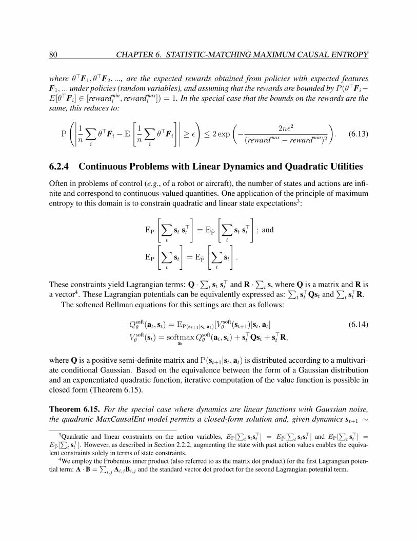
80 CHAPTER 6. STATISTIC-MATCHING MAXIMUM CAUSAL ENTROPY
where θ>F1, θ>F2, ..., are the expected rewards obtained from policies with expected features
F1, ... under policies (random variables), and assuming that the rewards are bounded by P (θ>Fi−E[θ>Fi] ∈ [rewardmin
i , rewardmaxi ]) = 1. In the special case that the bounds on the rewards are the
same, this reduces to:
P
(∣∣∣∣∣ 1n∑i
θ>Fi − E
[1
n
∑i
θ>Fi
]∣∣∣∣∣ ≥ ε
)≤ 2 exp
(− 2nε2
(rewardmax − rewardmin)2
). (6.13)
6.2.4 Continuous Problems with Linear Dynamics and Quadratic Utilities
Often in problems of control (e.g., of a robot or aircraft), the number of states and actions are infi-nite and correspond to continuous-valued quantities. One application of the principle of maximumentropy to this domain is to constrain quadratic and linear state expectations3:
EP
[∑t
st s>t
]= EP
[∑t
st s>t
]; and
EP
[∑t
st
]= EP
[∑t
st
].
These constraints yield Lagrangian terms: Q ·∑
t st s>t and R ·∑
t s, where Q is a matrix and R isa vector4. These Lagrangian potentials can be equivalently expressed as:
∑t s>t Qst and
∑t s>t R.
The softened Bellman equations for this settings are then as follows:
Qsoftθ (at, st) = EP(st+1|st,at)[V
softθ (st+1)|st, at] (6.14)
V softθ (st) = softmax
atQsoftθ (at, st) + s>t Qst + s>t R,
where Q is a positive semi-definite matrix and P(st+1|st, at) is distributed according to a multivari-ate conditional Gaussian. Based on the equivalence between the form of a Gaussian distributionand an exponentiated quadratic function, iterative computation of the value function is possible inclosed form (Theorem 6.15).
Theorem 6.15. For the special case where dynamics are linear functions with Gaussian noise,the quadratic MaxCausalEnt model permits a closed-form solution and, given dynamics st+1 ∼
3Quadratic and linear constraints on the action variables, EP[∑
t sts>t ] = EP[∑
t sts>t ] and EP[∑
t s>t ] =EP[
∑t s>t ]. However, as described in Section 2.2.2, augmenting the state with past action values enables the equiva-
lent constraints solely in terms of state constraints.4We employ the Frobenius inner product (also referred to as the matrix dot product) for the first Lagrangian poten-
tial term: A · B =∑
i,j Ai,jBi,j and the standard vector dot product for the second Lagrangian potential term.

6.3. RELATION TO ALTERNATE INFORMATION-THEORETIC APPROACHES 81
N(Ast + Bat,Σ), Equation 2.10 reduces to:
Qsoftθ (at, st) =
[atst
]> [ B>DB A>DBB>DA A>DA
] [atst
]+
[atst
]> [ B>GA>G
]V softθ (st) = s>t (Cs,s + Q− C>a,sC
−1a,aCa,s)st + s>t (Fs + R) + const,
where C and D are recursively computed as: Ca,a = B>DB; Cs,a = C>a,s = B>DA; Cs,s =
A>DA; D = Cs,s + Q− C>C−1a,aCa,s; and G = Fs + R.
The maximum causal entropy policy for the linear-quadratic setting is then distributed accordingto: P (at|st) ∝ eQ
softθ (at,st), which is also Gaussian.
6.2.5 Deterministic Dynamics ReductionThe inverse optimal control problem generalizes existing techniques for maximum entropy. Theconditional random field (Lafferty et al., 2001) is a common example. When the conditional distri-bution of side information (i.e., the state transition dynamics) is deterministic, the causal entropy(with static conditioning on features, {fs,a}) reduces to the conditional entropy (Theorem 4.22).The optimization of Equation 6.1 reduces in this setting to the following optimization:
maxA
H(A|{fs,a}) (6.15)
such that: EP(A)
[∑t
fst,at
]= EP(A)
[∑t
fst,at
]∑
A
P(A) = 1.
The form of the distribution over action sequences satisfying this optimization is:
P(A) ∝ e∑t θ>fst,at . (6.16)
When we consider the characteristics, {fs,a}, as variables on which the distribution is conditioned,this probability distribution corresponds to a conditional random field (Lafferty et al., 2001) whereeach At variable is conditioned on all characteristics, {fs,a} (though it only depends on the set offeatures associated with the value it takes on). This application of conditional random fields differsfrom typical applications, which are typically concerned with recognition of a sequence of hiddenvariables from a sequence of noisy observations.
6.3 Relation to Alternate Information-Theoretic ApproachesA natural question in the statistic-matching/inverse optimal control setting is: what benefits doesthe principle of maximum causal entropy provide compared to existing maximum joint, marginal,

82 CHAPTER 6. STATISTIC-MATCHING MAXIMUM CAUSAL ENTROPY
and conditional entropy approaches? We investigate this question in this section by exploringmaximum entropy approaches based on previous information-theoretic concepts.
6.3.1 Maximum Joint EntropyA natural approach to attempt is to maximize the joint entropy of S and A. We note the decom-position of the joint distribution into two causal distributions relates the joint entropy to the causalentropy (Remark 4.21). This decomposition shows the difference between these two measures—the extra causally conditioned side information entropy, H(ST ||AT−1):
H(A,S) = H(AT ||ST ) +H(ST ||AT−1). (6.17)
A simple application of the maximum joint entropy approach is to employ the Markov randomfield joint distribution,
P(A,S) ∝ eθ>F(S,A), (6.18)
and obtain a conditional probability distribution by marginalizing the latent future state variablesof the joint distribution:
P(At|S1:t,A1:t−1) ∝∑
St+1:T ,At+1:T
eθ>F(S,A).
Unfortunately this probability distribution is inefficient to compute and it ignores the crucial de-pendence between sequences with shared prefixes, which prevents two similar sequences fromhaving probability distributions that are independent from one another.
6.3.2 Causally-Constrained Maximum Joint EntropyA more sophisticated approach employs the causal constraints of the maximum causal entropyformulation on the joint entropy measure. The joint entropy is maximized while constrainingthe joint probability distribution to factor into the unknown causally conditioned probability of Agiven S, P(AT ||ST ), and the known causal conditional probability of S given A, P(ST ||AT−1), asfollows:
argmax{P(At|S1:t,A1:t−1)}
H(A,S) (6.19)
such that: EP(S,A)[F(S,A)] = EP(S,A)[F(S,A)]
∀S1:t,A1:t P(At|S1:t,A1:t−1) ≥ 0; and
∀S1:t,A1:t−1
∑At
P(At|S1:t,A1:t−1) = 1.

6.3. RELATION TO ALTERNATE INFORMATION-THEORETIC APPROACHES 83
The form of the conditional probability distribution satisfying this optimization is then:
Pθ(At|S1:t,A1:t−1) ∝ exp{θ> EP(S,A)[F(S,A)|S1:t,A1:t]
−∑τ>t
EP(S,A)[log Pθ(Aτ |S1:τ ,A1:τ−1) + log P(Sτ |S1:τ−1,A1:τ−1)|S1:t,A1:t]}. (6.20)
Relating this distribution to the Bellman equation (Bellman, 1957), we have:
QCCJE(at, st) , EP(st+1|st,at)[VCCJE(st+1)|st, at] + θ>fst,at +H(st+1|st, at) (6.21)
V CCJE(st) , softmaxat
QCCJE(at, st).
The key difference from the maximum causal entropy soft-maximum interpretation is the inclusionof the entropy associated with the state transition dynamics, H(st+1|st, at). Including this entropycan only decrease the uncertainty over action sequences. We argue that this is inappropriate whenthe dynamics of side information, P(ST ||AT−1), are known, or simply not variables of interest inthe prediction task.
Figure 6.3: A Markov decision process that illustrates the implications of considering the uncertainty ofstochastic dynamics under the causally conditioned maximum joint entropy model. Two actions are availablein state S1: one that has a high degree of next state uncertainty (top) and one that has a deterministic nextstate (bottom).
Figure 6.3 illustrates the sensitivity of the action distribution to the entropy of state transitiondynamics. As the number of stochastic next states in the top action increases, the action distri-bution under the causally constrained maximum joint entropy is biased heavily towards that topaction. However, this causally conditioned joint entropy could be appropriate for settings whereboth conditioned and side information distributions are being estimated. We do not investigate thatsetting in detail in this thesis.

84 CHAPTER 6. STATISTIC-MATCHING MAXIMUM CAUSAL ENTROPY
6.3.3 Marginalized Maximum Conditional EntropyWe previously showed how the conditional random field can be derived by maximizing the condi-tional entropy of a probability distribution subject to feature-matching constraints in Section 5.1.3.The resulting probability distribution is of the form:
P(A|S) ∝ e∑t θ>fat,st . (6.22)
Since the future state variables, St+1:T , are unavailable when At is predicted, a practical approachis to take the joint distribution using Equation 6.22 and the transition dynamics and marginalizeover the latent future state:
P(at|st) ∝∑
st+1:T
∏τ>t
P(sτ+1|sτ , aτ )e∑τ θ>faτ ,sτ
=∑
st+1:T
e∑τ θ>faτ ,sτ+log P(sτ+1|sτ ,aτ ) (6.23)
Theorem 6.16. The marginalized maximum conditional entropy distribution (Equation 6.23) canthen be interpreted under the dynamic programming perspective using the re-expression:
QCEθ (at, st) = softmax
st+1
(V CEθ (st+1) + log P(st+1|st, at)
)+ θ>fat,st (6.24)
V CEθ (st) = softmax
atQCEθ (at, st)
If we view the Lagrangian potential function, θ>fat,st , as a reward, then under this model anadditional cost of − log P(St+1|S1:t,A1:t) is “paid” to obtain the desired outcome from the tran-sition dynamics. As a result, the recovered policy is not equivalent to the corresponding Markovdecision process’ optimal policy.
Remark 6.17 (based upon Toussaint (2009), Equation 12). By Jensen’s inequality, the log likeli-hood of the conditional random field distribution (Equation 3.2) corresponds to an upper boundon the expected reward (i.e., negative expected cost) in the corresponding MDP rather than theexact expected reward:
log ES,A
[T∏t=0
e−cost(At,St)∣∣∣π(A|S)
]≥ ES,A
[log
T∏t=0
e−cost(At,St)∣∣∣π(A|S)
](6.25)
= ES,A
[−
T∑t=0
cost(At, St)∣∣∣π(A|S)
].

6.4. DISCUSSION 85
Figure 6.4: A Markov decision process that illustrates the preference of the marginalized maximum condi-tional entropy for “risky” actions that have small probabilities of realizing high rewards. Consider actionsin the four cardinal directions from each state (i.e., grid cell), and transition dynamics that with some prob-ability of failure, a transition is made to an orthogonal cardinal direction instead of the intended direction.Green cells have very low cost, gray cells have medium, and red cells have extremely high cost.
The relationship between these two objectives is shown in Remark 6.17. Thus, the model hasa strong preference for sequences of actions where the expected utility obtainable by any actualpolicy is quite low (due to the stochastic transition dynamics leading to low-reward outcomes), buta few “lucky” sequences have high utility.
This preference for risky state dynamics is illustrated in Figure 6.4, where a high utility tra-jectory to a goal state is possible, but unlikely due to stochastic state transition dynamics. Thosedynamics make an alternate policy—going “around” rather than taking the risky path—have higherexpected utility, but that policy is less preferred under the marginal maximum conditional entropymodel, which assumes that desirable state transitions can be realized by paying a penalty.
6.4 DiscussionIn this chapter, we have derived the probability distribution of the maximum causal entropy dis-tribution for the statistic-matching constraint setting. We have shown that the problem of inverseoptimal control can be posed in this way, and that the Lagrangian potentials, θ>f, that result canbe interpreted as analogs to rewards or costs in existing decision frameworks. This connection issignificant: prediction of purposeful behavior follows the same mechanisms as optimal generationapproaches for that behavior (with added relaxations to address uncertainty). It is also surprising:after beginning with a purely information-theoretic formulation of an estimation problem, we havearrived at a stochastic generalization of optimal control criteria.
Other work has similarly aimed at combining information theory with decision theory and

86 CHAPTER 6. STATISTIC-MATCHING MAXIMUM CAUSAL ENTROPY
warrants discussion. One prevalent line of research is determining the value of information, whichis the amount an agent in a decision framework would be willing to pay to observe the value of avariable before making a decision (Howard, 1966; Poh & Horvitz, 1996; Krause & Guestrin, 2005).This perspective is useful for prescriptive purposes, but not for the predictive task we addresswith the maximum causal entropy approach. Tishby & Polani (2010) define an information-to-goquantity as an information-theoretic analog of the decision-theoretic cost-to-go. It is a measureof the future uncertainty of states and actions in decision settings, relative to a prior belief aboutthe marginal distributions of future states and actions. This is similar to the causally-constrainedmaximum joint entropy approach and suffers the same bias for highly uncertain state transitiondynamics. However, it may be useful if predicting both the future actions and states is desired.

Chapter 7
Maximum Causal Entropy InfluenceDiagrams for Imperfect Information
“Real knowledge is to know the extent of one’s ignorance.”— Confucius (Philosopher, 551–479BC).
In the previous chapter, we investigated reasoning in the presence of future uncertainty. Manyapplications of machine learning and decision making also involve reasoning in the presence ofhistoric and current uncertainty. For example, in partially observable Markov decision processes(POMDPs), only noisy observations of the world’s state are revealed to the agent, and the agentis forced to act based on an uncertain belief about the world. This chapter extends the maximumcausal entropy approach to settings with side information that includes latent variables and prob-lems with imperfect recall where past observations are “forgotten.” We employ a maximum causalentropy variant of the influence diagram (Miller et al., 1976; Howard & Matheson, 1984), a graph-ical framework that subsumes Bayesian Networks and augments their capabilities to reason aboutlatent variables with decisions and utilities so that inference includes optimal decision making.
Maximum causal entropy expands the applicability of influence diagrams from the prescriptionof optimal decisions to the prediction of decision-making and the recovery of explanatory utilityweights from observed decision sequences. Additionally, influence diagrams provide a convenientgraphical representation of variable relationships in behavior prediction tasks. We investigate thestructural properties of influence diagrams required for the maximum causal entropy approach tobe applicable, finding that perfect decision recall is required.
7.1 Maximum Causal Entropy Influence DiagramsWe begin by describing different types of imperfect information and examples for each to moti-vate the contributions of this chapter before introducing the maximum causal entropy influencediagram.
87

88 CHAPTER 7. MAXIMUM CAUSAL ENTROPY INFLUENCE DIAGRAMS
7.1.1 Imperfect InformationSupporting the additional uncertainty of latent variables from the current point in time and fromthe past extends the maximum causal entropy model to behavior prediction in partial information,multi-player, and bounded rationality settings. For example, in many multi-player games (e.g.,card games such as poker), each player possesses a partial and distinctive knowledge of the stateof the game and acts by inferring the other players’ knowledge. Explicitly modeling this dynamicinformation availability is important for the prediction of actions in such settings.
We consider four different types of imperfect information in sequential decision settings:
1. Latent future side information: Future side information variables, Xt+1:T , are unavailablewhen each conditioned variable, Yt, is chosen. Example: the maximum causal entropy in-verse optimal control setting of Chapter 6 (e.g., control of a system in settings with stochasticdynamics).
2. Partially observed side information: Side information variables, X1:t, are only partiallyobserved at each time step. Example: behavior in a partially observable Markov decisionprocess (e.g., the exploratory diagnosis of a partially-observed system).
3. Latent previously observed side information: Conditioning variables from the parent setof an early conditioned variable, par(Yt1), that are relevant to a future conditioned variable,Yt2 (t1 < t2), but “forgotten” and not part of the parent set of Yt2 . Example: games whereplayers have secret information (e.g., simple variants of poker).
4. Latent past decisions: Earlier conditioned variables (Yt1), that are relevant to future condi-tioned variables, Yt2 (t1 < t2), but “forgotten” and not part of the parent set of Yt2 . Example:multi-player games with hidden (or simultaneous) actions in otherwise full information set-tings.
In this chapter, we discuss the applicability of the maximum causal entropy approach to thelatter three information settings. We generalize the dependency structure of maximum causal en-tropy inverse optimal control from Chapter 6 to address the second and third imperfect informationsettings.
7.1.2 Representation: Variables, Dependencies, and FeaturesWe employ the influence diagram graphical model structure as a convenient representation for theestimated variables (Y), the conditioning variables (X), and the feature functions, F(X,Y). Weagain employ the decision-based interpretation of these variables, replacing Y with actions, A, andX with state variables, S.
The maximum causal entropy influence diagram differs from the traditional influence diagram(Section 2.2.3) primarily in the meaning of utilities.

7.1. MAXIMUM CAUSAL ENTROPY INFLUENCE DIAGRAMS 89
Definition 7.1. A maximum causal entropy influence diagram (MaxCausalEnt ID) is structurallycharacterized by three different types of nodes and directed edges connecting those nodes. Thenode types are:
• Square decision nodes (A) that correspond to conditioned variables;
• Circular uncertainty nodes (S) that correspond to observed and unobserved side informationvariables; and
• Diamond utility nodes (U) that correspond to statistic-matching potential functions.
Additionally, directed edges connect these nodes with the role of each edge depending on the typeof node to which it is a parent1. The roles are as follows:
• The parents of a decision node, par(At), are conditioned on or “known” when the At vari-able is assigned an instantiation value.
• An uncertainty node’s parents, par(St), specify the variables upon which its conditionalprobability distribution, P(St|par(St)), is defined.
• The parents of a utility node, par(Ut), in a MaxCausalEnt ID indicate the form of featurefunctions of the utility node FUt : par(Ut)→ Rk.
The variables and relationships of the maximum causal entropy influence diagrams are summarizedin Table 7.1.
Table 7.1: Influence diagram graphical representation structural elements, symbols, and relationships.
Type Symbol Parent relationship
Decision nodesSpecifies the variables that are observed when action A is se-lected
Uncertainty nodesSpecifies the conditional probability distribution, P(S|par(S)),of the state variable S
Utility nodesSpecifies feature utility functions, θ>F (par(U))→ R, with (un-known) parameter weights θ
The only requirement on the structure of a maximum causal entropy influence diagram isacyclicity. However, the complexity of reasoning in the MaxEnt ID depends greatly on the de-pendencies between decision distributions implied by the structure (i.e., the other decision distri-butions that are required to infer a particular decision node’s distribution). Instead, those problemscan often be more efficiently solved by exploiting the factored distribution of the side information.
1We assume utility nodes are not parents of any other node, but the same desired relationship—knowing whatutility is received—can be accomplished by employing an intermediary uncertainty node that takes on the utility.

90 CHAPTER 7. MAXIMUM CAUSAL ENTROPY INFLUENCE DIAGRAMS
7.2 Maximum Causal Parent Entropy
Using the structure of the influence diagram, we now formulate the corresponding maximum causalentropy optimization, the structural constraints required by the formulation, and the probabilitydistribution form.
7.2.1 Formulation and Optimization
We formulate the imperfect information maximum causal entropy optimization problem by allow-ing a distribution over side information variables, X, and conditioned variables, Y, that forms ajoint distribution as:
P(Y,X) =∏t
P(Yt|par(Yt))∏t
P(Xt|par(Xt)), (7.1)
where par(Yt) ⊆ (Y1:t−1∪X) represents a set of parent variables of Yt, and par(Xt) are constrainedso that the directed graph formed by edges {epar(Yt)→Yt} ∪ {epar(Xt)→Xt} is acyclic.
Extending the setting of Chapter 5, we assume that the conditional distribution of side informa-tion, P(X||par(X)), is known, and we are left to estimate the conditional distribution, P(Y||par(Y)).
The causally conditioned probability distribution and entropy measure extend to this influencediagram graphical structure setting.
Definition 7.2. We define the causal parent probability of Y given X as:
P(Y||par(Y)) ,∏t
P(Yt|par(Yt)). (7.2)
Definition 7.3. The causal parent entropy is formed from this probability distribution and is:
H(Y||par(Y)) , EP(X,Y)[− log P(Y||par(Y))]. (7.3)
This entropy measure serves as the objective function that extends the maximum causal en-tropy approach to settings with additional imperfect information. The key distinction between thisentropy measure and the previous causal entropy measure (Equation 4.13) introduced in Chapter4 is that some of the variables in X may never be directly conditioned upon by any Y variable ormay be conditioned on intermittently (along with past Y variables) over time in the causal parententropy measure of this section.
Definition 7.4. The imperfect information maximum causal entropy optimization maximizes thecausal parent entropy (Equation 7.3) while matching expected and statistic-based feature func-

7.2. MAXIMUM CAUSAL PARENT ENTROPY 91
tions, F(X,Y)→ RK . It is formally defined as:
max{P(Yt|par(Yt))}
H(Y||par(Y)) (7.4)
such that: EP(X,Y)
[∑t
Ft(X1:t,Y1:t)
]= EP (X,Y)
[∑t
Ft(Xt, Yt)
]∀t,Yt,par(Yt) P(Yt|par(Yt)) ≥ 0
∀t,par(Yt)
∑Yt
P(Yt|par(Yt)) = 1.
Just as in the general maximum causal entropy optimization (Equation 5.6), the convexity ofthe imperfect information optimization (Equation 7.4) when optimizing in terms of the conditionalprobability terms, {P(Yt|par(Yt))}, is not readily apparent. Indeed, only with further restrictionsto the parent structure of variables do we establish the convexity of the optimization in Equation7.4.
Definition 7.5. Perfect past decision recall is a constraint on the parent sets of decision variables,Y, that forces all past decision variables to be parents of future decision variables:
∀t Y1:t−1 ⊆ par(Yt). (7.5)
Convexity follows from the additional constraint of perfect decision recall (Definition 7.5).
Theorem 7.6. The imperfect information maximum causal entropy optimization of Equation 7.4constrained by perfect past decision recall can be formulated as a convex optimization problem.
Proof (sketch). Consider the causal conditional probability distribution, {P(YT ||XT )}, of a partic-ular conditioned variable, Yt, its parent set, par(Yt), and the variables that are greater-ancestors(i.e., non-parent ancestors of Yt):
granc(Yt) , anc(Yt) ∩ par(Yt).
As before, future side information variables can have no causal influence over earlier conditionedvariables; this is accomplished using the final constraints of Equation 5.6—marginalizing overnon-ancestor variables. This constrains the causally conditioned probability distribution to factorinto a product of ancestor-conditioned terms:
P(Y||X) =∏t
P(Yt|par(Yt), granc(Yt)).
Of the ancestor values in each conditional probability term: P(Yt|par(Yt), granc(Yt)), the grancset of variables are unobserved. Constraining these conditional probability distributions to beequivalent across varying greater-ancestor values,
∀t,Yt,par(Yt),granc(Yt)1,granc(Yt)2 P(Yt|par(Yt), granc(Yt)1) = P(Yt|par(Yt), granc(Yt)2),

92 CHAPTER 7. MAXIMUM CAUSAL ENTROPY INFLUENCE DIAGRAMS
enforces any imperfect information constraints that are implied by the variable dependence struc-ture. When constrained by perfect past decision recall, this constraint is a linear function ofcausally conditioned probabilities.
Remark 7.7. Without perfect past decision recall, the imperfect information maximum causalentropy optimization is non-convex in general.
This property of perfect decision recall denotes an important boundary for the applicability ofthe causal entropy approach; without it, convexity and strong duality, upon which the maximumentropy approach relies, do not hold (Remark 7.7). The inefficiency of reasoning in the generalimperfect past decision setting should not be particularly surprising; it could be employed to rep-resent Nash equilibria inference problems in a wide range of game settings that are known to benon-polynomial (assuming the complexity hierarchy does not collapse).
7.2.2 Distribution FormFollowing the formulation of Theorem 7.6, we obtain the form of the distribution for the imperfectinformation setting with perfect past decision recall.
Theorem 7.8. The maximum causal entropy probability distribution for the imperfect informationsetting with perfect past decision recall (Theorem 7.6) is distributed according to the followingrecurrence relationship:
Pθ(Yt|par(Yt)) =ZYt|par(Yt),θ
Zpar(Yt),θ(7.6)
logZpar(Yt),θ = log∑Yt
ZYt|par(Yt),θ
= softmaxYt
(EP(par(Yt+1)|par(Yt),Yt)
[logZpar(Yt),θ|par(Yt), Yt)
] )ZYt|par(Yt),θ = e(EP(par(Yt+1)|par(Yt),Yt)[logZpar(Yt),θ|par(Yt),Yt)])
Zpar(YT+1),θ = eθ>F(X,Y),
where the final set of parents for the “after last” Y variable is the complete set of variables:par(YT+1) , X ∪ Y.
It is similar to the feature-matching maximum causal entropy distribution, except that addi-tional variables can be latent and are then marginalized over given the parents of each Yt.
7.2.3 Perfect Recall ReductionOne important special case of imperfect information that simplifies the distribution of Equation7.6 is perfect recall, which limits uncertainty to side information variables that will be revealed at

7.2. MAXIMUM CAUSAL PARENT ENTROPY 93
some point in time (or are never revealed). This specifically excludes past decisions or influenceson decisions that are later “forgotten.”
Definition 7.9. In the perfect recall sequential prediction setting, each conditioned variable, Yt, isconstrained to be conditioned on all previous conditioned variables and variables on which theydepended. This constrains the parent sets as follows:
∀t par(Yt) ∪ Yt ⊆ par(Yt+1). (7.7)
Imperfect information modeling problems with perfect recall structure (Definition 7.9) can bereduced to the maximum causal entropy inverse optimal control setting of Chapter 6 via Theorem7.10.
Theorem 7.10. In the perfect recall setting, the imperfect information maximum causal entropydistribution of Equation 7.4 can be reduced to a non-latent maximum causal entropy model byemploying expectations to obtain side information dynamics,
P ′ (par(Yt)|Yt−1, par(Yt−1)) =
EP(X|Yt−1,par(Yt−1))
[P(par(Yt)|X, Yt−1, par(Yt−1)) P(X|Yt−1, par(Yt−1))
∣∣Yt−1, par(Yt−1)],
and expected statistic-based features,
F ′t (Yt, par(Yt)) = EP(X|par(Yt))[Ft(X,Y1:t−1)) P(X|par(Yt))
∣∣par(Yt)].
Additionally, strict perfect recall is often not necessary; parent sets that satisfy perfect recallcan often be reduced without affecting the corresponding maximum causal entropy probabilitydistribution.
Definition 7.11. A subset of conditioning variables, parC(Yt) ⊆ par(Yt), (i.e., side information, X,or previous conditioned variables, Y1:t−1,) is relevant in the maximum causal entropy setting if itis the minimum size set of variables such that:
P(Yt|par(Yt)) = P(Yt|parC(Yt)),
where parC(Yt) is the set of parents for Yt that are members of set C, and P(Yt|parC(Yt)) is thedistribution obtained by maximizing the causal parent entropy (Equation 7.4) according to thisalternate conditioning structure.
Any parents of a conditioned variable that are not relevant (Definition 7.11) can be removedfrom the parent set, reducing the complexity of the resulting maximum causal entropy model’sparametrization.

94 CHAPTER 7. MAXIMUM CAUSAL ENTROPY INFLUENCE DIAGRAMS
7.3 Example Maximum Causal Entropy Influence Diagram Rep-resentations
Many sequential data modeling problems can be expressed as maximum causal entropy influencediagrams. This is a natural consequence of many optimal control problems being representable asinfluence diagrams (Section 2.2.3). We now review a few classes of decision prediction tasks toillustrate the breadth of applicability of the maximum causal entropy influence diagram.
Figure 7.1: The maximum causal entropy influence diagram graphical representation for maximum causalentropy inverse optimal control. For Markov decision processes: Ut(St, At) = θ>fSt,At , and for linearquadratic regulation models: Ut(st, at) = s>t Qst + a>t Rat. Absolute conditioning on {fS,A} or Q and R issuppressed, as are perfect recall dependencies that are irrelevant.
The model of maximum causal entropy inverse optimal control (Chapter 6) is depicted in Figure7.1. The Markov decision process and linear quadratic regulation settings can each be representedwith different forms of utility node functions. Note that perfect past decision recall edges arenot present. However, descendants’ utility nodes are conditionally independent of past decisionsgiven parents of an action. Thus, past decisions are irrelevant and the perfect past decision recallrequirement is not violated.
The fully observable control prediction task of Figure 7.1 is extended to the setting where thestate is only partially-observed through observation variables in Figure 7.2. This model satisfiesthe perfect recall constraint since all influences on past decisions and decisions are parents of futuredecision nodes.

7.3. EXAMPLE REPRESENTATIONS 95
Figure 7.2: The maximum causal entropy influence diagram graphical representation for maximum causalentropy inverse optimal control in a partially observable system. The state variables are only partiallyobserved via observation variables, O1:T , that are distributed according to a known conditional distribution,P(Ot|St).
Figure 7.3: The extensive-form game setting where players have access to private information, S1 and S2,and take sequential decisions. Recall of all past actions is provided by the sets of edges connecting alldecisions.
Figure 7.3 shows a maximum causal entropy influence diagram for an extensive-form gamewhere each player has private information that is only conveyed to the other players through achoice of actions. The decision problem of this influence diagram satisfies the perfect past decisionrecall property.

96 CHAPTER 7. MAXIMUM CAUSAL ENTROPY INFLUENCE DIAGRAMS
Figure 7.4: The Markov game setting where the state of the game changes according to known Markovianstochastic dynamics, P(St+1|St, At,1, At,2), and the players share a common reward.
Figure 7.4 shows a maximum causal entropy influence diagram for a Markov game settingwhere two players act simultaneously without knowing the other player’s action. This setting doesnot satisfy the perfect decision recall property because At,1 and At,2 have no recall relationship.We investigate settings where the actions at each timestep are correlated in Chapter 8.
7.4 DiscussionIn this chapter, we have expanded the maximum causal entropy approach for matching empiricalstatistics of data to settings where in addition to future latent variables, past and current variablescan be latent also.
The four imperfect information settings are covered to various degrees by the maximum causalentropy formulations introduced thus far, as shown in Table 7.2.
Table 7.2: Coverage of the four imperfect information settings by different maximum causal entropy vari-ants.
Lat
entf
utur
ein
form
atio
n
Part
ial
obse
rvab
ility
Lat
entp
ast
cond
ition
ing
Lat
entp
ast
deci
sion
s
Inverse optimal control maximum causal entropy XPerfect recall maximum causal entropy X X
Perfect past decision recall maximum causal entropy X X XImperfect recall maximum causal entropy X X X X

7.4. DISCUSSION 97
The perfect recall maximum causal entropy formulation (Definition 7.9) has the advantage ofreducing to the inverse optimal control model, making inference relatively straight-forward. Theperfect past decision recall formulation extends the applicability to settings where side informationon which past decisions were based is latent. Finally, the imperfect information maximum causalentropy formulation (Definition 7.4) supports all of these forms of imperfect information, but is nolonger a convex optimization problem.
The problem of recovering explanatory utility functions for influence diagrams was previouslyinvestigated for inconsistent behavior by assuming for each instance of behavior, a noisy copy ofthe true utility function was sampled and then optimal behavior under that noisy utility functionemployed to obtain the demonstrated behavior sequence (Nielsen & Jensen, 2004). Markov chainMonte Carlo techniques are then employed to learn the mean and variance of the distribution fromwhich noisy utility functions are drawn. We view the maximum causal entropy influence diagram asignificant improvement over this inefficient learning procedure since the convexity of its objectivefunction enables much more efficient and more exact learning.

Chapter 8
Strategic Decision Prediction via MaximumCausal Entropy
“Maybe all one can do is hope to end up with the right regrets.”— Arthur Miller (Playwright, 1915–2005).
In this chapter, we investigate settings where multiple agents or players take actions withinsequential stochastic games. Equilibria solution concepts, such as Nash equilibria (NE) (Nash,1951) and correlated equilibria (CE) (Aumann, 1974) are important constructs for these gamesthat provide certain individual or group performance guarantees. However, from a machine learn-ing perspective, existing equilibria concepts are often not useful for prediction, because they donot fully specify a unique strategy profile. Instead they may specify a polytope or point set ofpossible expected utility outcome vectors, making strategy prediction under-specified in generalwithout additional assumptions. We introduce the maximum causal entropy correlated equilib-ria solution concept for predictive purposes based on the principle of maximum causal entropywith rationality constraints that prevent any regret from changing actions from that prescribed bythe joint distribution in this chapter.
8.1 Game Theory Background
8.1.1 Classes of GamesThe canonical type of game studied within game theory is the one-shot game with a matrix ofpayoffs for the players (Definition 8.1).
Definition 8.1. A normal-form game, GN , is defined by a set of players i = 1...N , a set of actionsfor each player, ai,j ∈ Ai, and a utility vector Ua1,j1 ,...,aN,jN ∈ RN , specifying the payoffs to eachplayer for every combination of actions.
98

8.1. GAME THEORY BACKGROUND 99
In a normal-form game, each player (i = 1...N ) selects an action (ai) simultaneously withoutknowledge of other players’ selected actions. A utility vector for each combination of actions,Ua1,j1 ,...,aN,jN ∈ R
N , specifies a numerical payoff, Ua,i, to each player (i).
Table 8.1: The prisoner’s dilemma normal-form game. Two prisoners jointly receive the minimal sentenceif they both remain silent, but each has an incentive to (unilaterally) confess.
Silence ConfessSilence 0.5 years, 0.5 years 10 years, 0 yearsConfess 0 years, 10 years 5 years, 5 years
The prisoner’s dilemma (Table 8.1) is a classic example of a normal form game.
Definition 8.2. A Markov game (Filar et al., 1997) (also known as a stochastic game) is definedby a set of states (S) representing the joint states of N players, a set of individual actions (A)for each player, a probabilistic state transition function, T : S × A1:N → P(S ′) specifying thedistribution for next state, S ′, and a utility function, Utilityi : S × A1:N → R for each playeri = 1 : N .
Markov games (Definition 8.2) generalize normal-form games to sequential action settings.They also generalize Markov decision problems by incorporating multiple players who act basedupon their individual utility functions and jointly influence the future state of the game with theiractions, as shown in Figure 8.1.
Figure 8.1: The sequence of states and (Markovian) actions of a Markov game. Actions at each time stepcan either be correlated (i.e., dependently distributed based on past actions and states or an external signalingdevice), or independent.
Definition 8.3. An extensive-form game is defined by a tree of action sequences and state out-comes where each agent is incapable of distinguishing between multiple states in the tree.

100 CHAPTER 8. STRATEGIC DECISION PREDICTION
Extensive form games (Definition 8.3) further extend the Markov game setting in a way whereunique sequences of states and actions may end up in a meta-state that is indistinguishable by theagent from other states. This allows situations with incomplete information, such as imperfectrecall, to be represented within the model.
Game players choose a strategy profile, π, specifying next actions for each situation thatare either mixed (stochastic) or pure (deterministic); and either correlated (joint functions) orindependent (factor by players) based on a (discounted, 0 < γ ≤ 1) cumulative expected utility:
ExpectUtilπi (at1:N , st) , Eπ(st+1:T ,at+1:T
1:N |at1:N ,st)
[∑τ≥t
γτUtilityi(sτ , aτ1:N)
∣∣∣∣∣at1:N , st, π
](8.1)
for player i under the joint strategy profile, π. We assume in Equation 8.1 and throughout thischapter that the strategy profile is mixed and Markovian1, meaning it depends only on the currentstate and timestep. In a stationary mixed strategy profile, the joint action probabilities for eachstate are the same for all time steps.
To obtain strategy profiles, it is useful to consider the amount of utility gained when takinga deviation action, ati
′, instead of a provided action, ati, when: all players’ actions except playeri’s, denoted at−i, are known (Equation 8.2); or when other players’ actions, at−i, are unknown andaveraged over according to the strategy profile (Equation 8.3):
ExpectDevGainπi (at1:N , st, ati
′) , ExpectUtilπi ({at−i, ati
′}, st)− ExpectUtilπi (at1:N , st) (8.2)
ExpectRegretπi (ati, ati′, st) , EPπ(at−i|at,st)
[ExpectDevGainπi (at1:N , s
t, ati′)∣∣∣ati, st] . (8.3)
These quantities are useful for assessing the rationality of multi-player strategies.
8.1.2 Equilibria Solution ConceptsDefining equilibria solution concepts and finding corresponding equilibria in multi-agent settingsare important problems for applications ranging from conflict resolution to market-making. Per-haps the most widely-known solution concept in game theory is the Nash equilibrium.
Definition 8.4. A Nash equilibrium for a game is defined as a fixed point where no agent haspositive deviation regret and agents’ actions are independent.
Though any finite game is guaranteed to have a mixed strategy Nash equilibrium (Nash, 1951),only exponential-time NE-finding algorithms are known to exist (Lemke & Howson Jr, 1964) forgeneral-sum normal-form games, and associated decision problems regarding the characteristicsof possible NE are NP-hard (Gilboa & Zemel, 1989).
1Markovian equilibria strategy profiles are a consequence of the MCECE formulation and a commonly assumedconstraint imposed on equilibria in other solution concept formulations.

8.1. GAME THEORY BACKGROUND 101
When extending equilibria from the normal-form setting to the dynamic setting of Markovgames, the concept of sub-game equilibria—that even in states that are not reached under a policy,the expected utilities of those states are based on the equilibrium of a game starting in that state—isan important requirement.
Definition 8.5. A correlated equilibrium (CE) (Aumann, 1974) for a Markov game is a mixed jointstrategy profile, πCE , where no expected utility gain is obtained for any player by substituting anaction, ati
′ that deviates from the strategy. This is guaranteed with the following set of constraints:
∀t,i,st,ati,ati ′ ExpectRegretπCE
i (ati, ati′, st) ≤ 0. (8.4)
Under this set of constraints, given the agent’s prescribed action, ati, there is no benefit for deviat-ing (under the distribution of other players’ actions, P (at−i|ati)). We further require that regrets bedefined according to sub-game correlated equilibria.
Unlike Nash equilibria (Nash, 1951), which require independent player strategies, players ina CE can coordinate their actions to obtain a wider range of expected utilities. Traffic lights area canonical example of a signaling device designed to produce CE strategies. However, externalsignaling mechanisms are not necessarily required—players can coordinate their actions from theirhistory of past actions in sequential game settings. The deviation regret constraints (Equation8.4) define a convex polytope of CE solutions in the N-dimensional space of players’ joint utilitypayoffs (Figure 8.2).
Figure 8.2: A correlated equilibria polytope with a correlated-Q equilibrium (Definition 8.6) payoff at pointA that maximizes the average utility and a maximum entropy correlated equilibrium at point B (Definition8.9) that provides predictive guarantees.
Consider the single shot, two-player prisoner’s dilemma of Table 8.1. For each of the twoplayers and two actions, there is one alternate action. Thus there are a total of four linear constraintsfor the prisoner’s dilemma setting (and more generally, any two-player, two-action normal-formgame).

102 CHAPTER 8. STRATEGIC DECISION PREDICTION
In general, for a single-shot (i.e., normal-form) game, there areO(N |A|2) regret constraints thatare linear in a total of O(|A|N) strategy variables, {π(a1:N)}, and CE solutions can be efficientlyobtained (i.e., in the same polynomial time as the size of the Utility matrix specification) by solvinga linear program (LP) or a convex program (CP):
maxπ
f0(π(A1:N)) (8.5)
such that: ∀i,ai,ai′∑a−i
π(a1:N)(Utility ({a−i, ai′})− Utility(a1:N)
)≤ 0,
∀a1:Nπ(a1:N) ≥ 0, and∑a1:N
π(a1:N) = 1.
depending on whether the objective function, f0, is linear or (negative) convex.
Definition 8.6. A correlated-Q equilibria (CE-Q) (Greenwald & Hall, 2003) employs a linear orconvex function of strategy probabilities for the selection metric objective of Equation 8.5 to obtainutility-unique strategy profiles2.
A number of objectives for CE-Q have been proposed (Greenwald & Hall, 2003):
• Utilitarian (uCE-Q) maximizes the sum of players’ utilities,∑N
i=1 Eπ[Utilityi(a1:N)];
• Dictatorial (dCE-Q) maximizes a specific player’s utility, Eπ[Utilityi(a1:N)];
• Republican (rCE-Q) maximizes the highest player’s utility, maxi Eπ[Utilityi(a1:N)]; and
• Egalitarian (eCE-Q) maximizes lowest player’s utility, mini Eπ[Utilityi(a1:N)].
These strong assumptions about players’ preferences constrain CE-Q solutions to reside on the hullof the most-positive quadrant of the CE polytope (Northeast in Figure 8.2). They do not necessarilyspecify a unique strategy profile or joint set of payoffs. However, they do specifically require that acorner of the joint utility polytope is covered by a CE-Q solution. More generally, strategies fromthe other polytope quadrants are also possible. Various forms of punishment, for example, suchas grim-trigger strategies, have been recognized as viable sub-game strategies that disincentivize aplayer’s undesirable actions. We augment these existing CE-Q with a few based on punishment:
• Disciplinarian (xCE-Q) minimizes a specific player’s utility, Eπ[Utilityi(a1:N)]; and
• Inegalitarian (iCE-Q) maximizes utility differences between two (groups of) different play-ers, Eπ[Utilityi(a1:N)− Utilityj(a1:N)].
2Unique strategy profiles are not guaranteed by the CE-Q solution concept—multiple actions can provide the samevector of player utilities, and the CE-Q strategies may comprise an entire facet of the CE polytope. We ignore thisambiguity and employ a single CE-Q from the set of CE-Q strategy profiles in this work.

8.2. MAXIMUM CAUSAL ENTROPY CORRELATED EQUILIBRIA 103
Definition 8.7. The maximum entropy correlated equilibria (MaxEntCE) solution concept fornormal-form games (Ortiz et al., 2007) selects the unique CE with the fewest additional as-sumptions (Figure 8.2) by employing Shannon’s information entropy as the objective function,−∑
a1:Nπ(a1:N) log π(a1:N), as advocated by the principle of maximum entropy (Jaynes, 1957).
Since a Nash equilibria is guaranteed to exist (Nash, 1951) and a Nash equilibria is a spe-cial case of correlated equilibria that is additionally constrained to have independent actions:P(a1:K) =
∏k P(ak), a correlated equilibria is always similarly guaranteed to exist. Of those
existing, one must maximize the entropy measure. However, the relaxation of the non-linear in-dependent action constraint that differentiates Nash equilibria from correlated equilibria enablesalgorithms to efficiently obtain correlated equilibria (Papadimitriou & Roughgarden, 2005) andmaximum entropy correlated equilibria (Ortiz et al., 2007) for a wider class of problems than canbe addressed using any algorithms for finding Nash equilibria (assuming the complexity hierarchydoes not collapse).
Table 8.2: The game of Chicken and its correlated equilibria strategy profiles.
Stay SwerveStay 0,0 4,1
Swerve 1,4 3, 3
CE 10 10 0
CE 20 01 0
CE 30 1
313
13
CE 414
14
14
14
Consider the game of Chicken (where each player hopes the other will Swerve) and the corre-lated equilibria that define its utility polytope in Table 8.2. CE 1 and CE 2 are both dictatorial andinegalitarian CE (for different players) and republican CE (but ambiguous). CE 3 is a utilitarianCE and an egalitarian CE. CE 4 is the maximum entropy CE. Its predictive guarantee is apparent:all other CE have infinite log-loss for at least one other CE; the MaxEntCE is the only CE thatassigns positive probability to the {Stay, Stay} action combination. We extend these predictiveguarantees to the Markov game setting in this work.
8.2 Maximum Causal Entropy Correlated Equilibria
We are motivated by two problems within the Markov game setting (Filar et al., 1997) characterizedby the dynamic interaction of multiple agents with a stochastic environment. The first is where atrusted third party (or signaling mechanism) must coordinate the behavior of agents in a way thatis both:
• A correlated equilibria that can be found efficiently; and
• Sensitive to the amount of information revealed about the agents’ underlying motives.

104 CHAPTER 8. STRATEGIC DECISION PREDICTION
The second is the problem of predicting the behavior of agents that are assumed to be actingaccording to an unknown correlated equilibria, which can naturally be arrived at without explicitcoordination by employing certain strategies in repeated games (Hart & Mas-Colell, 2000).
8.2.1 FormulationExtension of the MaxEntCE solution concept (Ortiz et al., 2007) to the Markov game setting is notstraight-forward. The first difficulty is that the deviation regret constraints of normal-form games(Equation 8.5), which are linear in the unknown mixed strategy variables, contain expectationsover future actions (Equation 8.4) when extended to the Markov game setting, creating non-linearconstraints that are products of the unknown variables.
Theorem 8.8. A linear program/convex program formulation of CE for Markov games is possi-ble by considering as variables the entire sequence of joint player actions for the sequence ofrevealed states, η(A1:T
1:N |S1:T ), and employing appropriate inequality constraints (deviation regretguarantees) and equality constraints (forcing the strategy over sequences to factor into products ofMarkovian strategies) on marginal distributions using linear functions of η(A1:T
1:N |S1:T ) variables.
Naıvely formulating the Markov game CE strategy profiles into an LP/CP is possible (Theorem8.8), but the number of constraints and variables grows exponentially with the time horizon3. Thesecond difficulty is that there are many entropy measures based on joint, conditional, and marginalprobability distributions that could be applied as objective functions. For example, the joint en-tropy is a natural entropy measure to consider. It is a combination of the entropy of the strategyprofiles’ actions and the entropy of the state dynamics:
H(a1:T1:N , s
1:T ) =T∑t=1
(H(at1:N |s1:t, a1:t−11:N ) +H(st+1|s1:t, a1:t
1:N)) = H(aT1:N ||sT ) +H(sT ||aT−11:N ).
(8.6)
Since the transition dynamics are already known in this problem setting, the uncertainty associ-ated with those dynamics is irrelevant. Maximizing the joint entropy generally makes the players’strategies less uncertain than otherwise possible by adding the assumption that players care aboutthe uncertainty that actions supply beyond expectations over their random outcomes. The reasonfor this extends directly from the decision theory setting illustrated by Figure 6.3 in Section 6.3.2.
We instead advocate the causally conditioned entropy measure (Kramer, 1998)H(AT1:N ||ST ) ,∑
tH(at1:N |a1:t−11:N , s1:t), employed throughout this thesis. For the possible sequences of states
and actions through a Markov game, it corresponds to the uncertainty associated with only theactions in such sequences. It is based on the causally conditioned probability distribution,
3The number of constraints is also exponential in the number of players. However, this is unavoidable in generalgame settings since the size of the payoff matrix grows exponentially with the number of players. We are thus onlyconcerned with reducing the exponential dependence on the time horizon in this work.

8.2. MAXIMUM CAUSAL ENTROPY CORRELATED EQUILIBRIA 105
P(AT1:N ||ST ) ,
∏t P(at1:N |a1:t−1
1:N , s1:t), which conditions each set of correlated actions only onactions and states that have been revealed at that point in time and not on future states, as in theconditional probability distribution P(A1:N |S) =
∏t P(at1:N |a1:t−1
1:N , s1:t, st+1:T ).
Definition 8.9. A maximum causal entropy correlated equilibrium (MCECE) solution maximizesthe causal entropy while being constrained to have no action deviation regrets4:
πMCECE , argmaxπ
H(aT1:N ||sT ) = argmaxπ
Ea1:T ,s1:T
[T∑t=1
− log P(at1:N |st)
](8.7)
such that: ∀t, i, ati, ati ′, st ExpectRegretπi (ati, ati′, st) ≤ 0
∀t, st, at1:N P(at1:N |st) ≥ 0, ∀t, st∑at1:N
P(at1:N |st) = 1,
π factors as: P(AT1:N ||ST ), and given: {P(st+1|st, at)}.
We further constrain the strategy profile to have sub-game equilibria, meaning that even in statesthat are unreachable under the strategy profile and state dynamics, the strategy profile is con-strained to satisfy Equation 8.7 in all sub-games starting from those states.
8.2.2 PropertiesBased on the view of conditional entropy as a measure of predictability (Cover & Thomas, 2006),the MCECE solution concept extends two important predictive guarantees to the multi-agent set-ting:
Theorem 8.10 (extension of (Ortiz et al., 2007)). Given an MCECE strategy profile, no player maydecrease the predictability of her action sequence without creating deviation regret for herself.
Theorem 8.11 (extension of (Grunwald & Dawid, 2003)). The MCECE solution strategy profile,πMCECE minimizes the worst-case log prediction loss for the sequences of joint actions, i.e.,
infP(AT ||ST )
supP (AT ||ST )
∑A,S
P (A,S) log P(AT ||ST ), (8.8)
of all the CE-satisfying deviation regret constraints, where P (AT ||ST ) is the (worst possible forprediction) empirical CE strategy and the joint, P (A,S), is the distribution of states and actionsunder that strategy profile and the known state transition dynamics.
4We employ a Markovian formulation for simplicity of presentation. Note that it arises without additional as-sumptions if a history-dependent strategy profile, P(at1:N |s1:t, a
1:t−11:N ), is employed, since the MCECE strategy profile
ultimately reduces to a Markovian strategy profile given the standard Markovian dynamics and Markovian payoffsassumptions of Markov games.

106 CHAPTER 8. STRATEGIC DECISION PREDICTION
Theorem 8.11 is particularly relevant to our machine learning perspective, because it justifiesthe MCECE strategy profile as a robust predictive model. It also provides a natural interpretationin gambling settings.
Remark 8.12. Given that players of a stochastic game behave according to some unknown corre-lated equilibrium, betting according to the MCECE distribution maximizes the worst-case growthrate of winnings in this setting.
Alternate entropy measures, such as the joint entropy, provide guarantees that are mathemati-cally similar to Theorem 8.10 and Theorem 8.11 but that do not match the Markov game setting.
Corollary 8.13 (of Theorem 8.8). The solution for the MCECE optimization (Equation 8.7) canbe obtained as the result of a convex program.
Despite being obtainable by convex optimization (Corollary 8.13), the straight-forward convexprogram is not practical due to its exponential growth in T . We present an efficient computationalformulation in Section 9.3.
8.2.3 Distribution FormWe obtain the general form of the MCECE distribution from its optimization. Despite the non-compact, history-dependent formulation of the naıve MCECE convex program, the strategy profilecan be expressed compactly for Markov games.
Lemma 8.14. The MCECE strategy profile for a Markov game is also Markovian.
Theorem 8.15. The MCECE strategy profile, πMCECEλ (at1:N |st), has the following recursive form
(with λ ≥ 0):
πMCECEλ (at1:N |st) ∝ e
−(∑
i,ati′ λi,st,ati,a
ti′ ExpectDevGainπ
MCECEi (at1:N ,st,ati
′))
+ExpectEnt(at1:N ,st), (8.9)
where ExpectEnt(at1:N , st) , Eat+1
1:N ,st+1
[ExpectEnt(at+1
1:N , st+1) +H(at+1
1:N |st+1)∣∣at1:N , s
t].
We discuss algorithms for recursively generating this distribution in Section 9.3.1 and for ob-taining λ parameters in a sequence of sub-problems for this recursion in Section 10.1.3.
8.3 DiscussionIn this chapter, we have applied the maximum causal entropy approach to multi-player sequentialgame settings. The result is a predictive model of correlated equilibrium strategy profiles thatprovides worst-case log-loss predictive guarantees in sequential game settings. This applicationdemonstrates the versatility of the maximum causal entropy approach to settings beyond standard
8.3. DISCUSSION 107
decision theory. It also illustrates the use of inequality constraints to enforce assumed rationalitycharacteristics of jointly rational behavior.
Dudık & Gordon (2009) previously applied maximum entropy to model behavior in extensive-form games. In that formulation, nature is treated as an additional player and the entropy associatedwith nature’s actions is also maximized. As we argued in Section 6.3.2, when the dynamics ofthe game are assumed to be common knowledge, maximizing this entropy introduces sensitivityto the transition dynamics and does not provide predictive guarantees of players’ strategies as aresult. Additionally, while extensive-form games generalize the classes of games we consider inthis chapter, strong duality does not hold; instead, only locally optimal model parameters trainedfrom data can be guaranteed.
8.3.1 Combining Behavioral and Rationality ConstraintsThe approach of this chapter is quite agnostic; no observed strategies are employed to predictfuture behavior. Given additional knowledge of past behavior, the employed rationality constraints(inequalities) can be augmented with behavioral constraints (equalities) that force the predictivedistribution to match demonstrated behavior strategies (in expectation) as in the inverse optimalcontrol setting of Chapter 6, and the maximum causal entropy influence diagram setting of Chapter7.
8.3.2 Infinite-horizon GamesExtending from finite-horizon to infinite-horizon games is not as straight-forward in the multi-player settings as it is in single-agent decision theory. Namely, asymmetric turn-taking behaviorarises as rational behavior in many games, and any finite-behavior game is then very sensitive to thespecific termination conditions of the game. Thus, approximating the infinite-horizon game witha very large finite-horizon game does not necessarily converge (Zinkevich et al., 2006). Murray& Gordon (2007) and MacDermed & Isbell (2009) attempt to efficiently extend value-iterationto propagate the entire polytope of correlated equilibria dynamically. Using approximations, thiscan be made efficient in practice. This approach holds promise for the maximum causal entropyapproach, but we do not investigate it in this thesis.

Part III
Algorithms
108

109
Overview of Part IIIPart III of this thesis leverages the theory of maximum causal entropy developed in Part II to for-mulate efficient algorithms for reasoning and training within the maximum causal entropy modelsof behavior.
Chapter 9 presents algorithms for efficient inferences of policies within the Markov decisionprocess, linear-quadratic regulation, and influence diagram frameworks and strategies within theMarkov game framework. Many of these algorithms are “softened” variants of the Bellman equa-tion or similar sequential dynamic programming algorithms.
Chapter 10 presents algorithms for training maximum causal entropy models from demon-strated behavior (or, in the case of multi-player game settings, simply to enforce rationality re-quirements). These algorithms are simple gradient-based optimization techniques that rely on theconvexity properties of the principle of maximum causal entropy from Part II to provide convergentoptimality guarantees.
Chapter 11 investigates the setting where observed behavior is chosen in pursuit of some goalknown to the actor but unknown to the observer. Bayesian inference methods are developed for in-ferring the latent goal with improved efficiency techniques for the non-adaptive (i.e., deterministicdynamics) special case.
The algorithms of these three chapters together enable the maximum causal entropy approachto be efficiently applied to large-scale behavior modeling and prediction tasks investigated in PartIV of this thesis.

Chapter 9
Probabilistic Inference
“Computers are useless. They can only give you answers.”— Pablo Picasso (Artist, 1881–1973).
We begin our exploration of algorithms for the maximum causal entropy approach by focusingour attention on the development and analysis of algorithms for the task of efficient inference givenmodel parameters within the maximum causal entropy models for feature expectation matching(Chapter 6), maximum causal entropy influence diagrams (Chapter 7), and predicting multi-agentactions (Chapter 8). Since approaches to parameter optimization (i.e., learning) within maximumcausal entropy models requires repeated inference for many different parameter values (Chapter10), efficient inference is especially important for the maximum causal entropy approach to beapplicable in large modeling domains.
9.1 Statistic-Matching Inference
We first consider inference algorithms for the statistic-matching setting of Chapter 6. As estab-lished by Theorem 6.8, there is a close connection between maximum causal entropy inferenceand stochastic optimal control based on a softened interpretation of the Bellman equation (Bell-man, 1957). Our algorithms are developed along this line of thought, with some important spe-cializations for the deterministic state transition dynamics setting, and significant differences inconvergence characteristics from optimal control algorithms.
9.1.1 Policy and Visitation Expectations
We are interested in two closely-related inference tasks:
• Obtaining the maximum causal entropy policy, π(A|S), for predictive purposes; and
110

9.1. STATISTIC-MATCHING INFERENCE 111
• Obtaining the expected number of times a certain state or action will be executed under thatpolicy, denoted Dsx or Dax,y for state x and action y in state x, respectively.
The latter quantities are needed to compute the statistics for model optimization purposes (e.g.,fitting to data).
From the soft Bellman equation interpretation of the maximum causal entropy distribution(Theorem 6.8), the policy is distributed according to:
π(a|s) = eQsoft(s,a)−V soft(s), . (9.1)
The state-action log partition function ,Qsoft(s, a), and the state log partition function, V soft(s),of Equation 9.1 are related by the following recurrence:
Qsoft(at, st) , logZat|st
= EP(st+1|st,at)[Vsoft(st+1)|st, at] + reward(st, at) (9.2)
V soft(st) , logZst
= softmaxat
Qsoft(at, st), (9.3)
where softmaxx f(x) , log∑
x ef(x).
We employ Algorithm 9.1 to dynamically compute the recurrence of Equation 9.2 and Equa-tion 9.3. A terminal state reward function, φ(s), influences or constrains the terminal state distri-bution of state-action sequences. For example, if φ(s) is negative infinity except for one particularstate, state-action sequences are then constrained to terminate in that state. The other goal settings(Section 6.1.5) can be similarly represented with appropriate choices of terminal state potentialfunction, φ(s).
For T iterations of the softmax propagation of Algorithm 9.1 (the loop beginning at line 4),the algorithm’s total running time is O(T |A||S|) for the case where each action has a non-zeroprobability of transitioning to each state. We will usually be concerned with settings where thenumber of possible next states for each action is bounded by a small constant. In that case, thetotal running time reduces to O(T (|A|+ |S|)).
We make frequent use of Algorithm 9.2 when performing exponentiated addition in the logspace. It avoids underflow and overflow when computing log partition functions and other relatedquantities.
The policy is then recovered from the state log partition function using Equation 9.1 and Equa-tion 9.2. We note that π(ax,y|sx) does not necessarily normalize over actions, i.e., often:∑
ax,y
π(ax,y|sx) < 1.
The remaining probability mass in any state that is not assigned to an action can be interpreted asan action that terminates the state-action sequence, which is distributed according to eφ(s)−V soft(s).

112 CHAPTER 9. PROBABILISTIC INFERENCE
Algorithm 9.1 State log partition function calculation
Require: MDP,MMDP, and terminal state reward function, φ(s)→ R.Ensure: state log partition functions, V soft(sx).
1: for all States sx do2: V soft(sx)← −∞3: end for4: while not converged do5: for all States sx do6: V soft(sx)
′ ← φ(sx)7: end for8: for all Actions ax,y do9: V soft(sx)
′ ← softmax(V soft(sx)
′, rewardMMDP(sx, ax,y) +∑
z P(sz|sx, ax,y)V soft(sz))
10: end for11: for all States sx do12: V soft(sx)← V soft(sx)
′
13: end for14: end while
Algorithm 9.2 Soft-maximum calculationRequire: inputs x1, x2
Ensure: softmax(x1, x2) = log (ex1 + ex2)1: maxx ← max(x1, x2)2: minx ← min(x1, x2)3: softmax(x1, x2)← maxx + log
(1 + eminx−maxx
)
We then arrive at a forward-backward inference algorithm that can be extended to approximate theinfinite time horizon.
From the policy action probabilities, a “forward pass” algorithm is employed to calculatevisitation frequencies for states and actions, as shown by Algorithm 9.3. Action visitation fre-quencies are easily recovered from state visitation frequencies and the stochastic policy, since:Dax,y = Dsxπ(ax,y|sx).
Similarly to Algorithm 9.1, the “forward” inference of Algorithm 9.3 is O(T |A||S|) in thefully connected transition dynamics case, and O(T (|A| + |S|)) when the number of next states isbounded by a constant.
Note that Algorithm 9.1 and Algorithm 9.3 strictly generalize the forward-backward algorithmfor efficient inference in Markov chain probability distributions (e.g., hidden Markov models, con-ditional random fields).

9.1. STATISTIC-MATCHING INFERENCE 113
Algorithm 9.3 Expected state frequency calculation
Require: MDP,MMDP, stochastic policy, π(ax,y|sx)), and initial state distribution P0(sx).Ensure: state visitation frequencies, Dsx under policy π(ax,y|sx).
1: for all states sx ∈MMDP do2: Dsx ← 03: end for4: while not converged do5: for all states sx ∈MMDP do6: D′sx ← P0(sx)7: end for8: for all actions ax,y ∈MMDP do9: for all states sz ∈MMDP reachable by ax,y do
10: D′sz ← D′sz +Dsx π(ax,y|sx) P(sz|ax,y, sx)11: end for12: end for13: for all states sx ∈MMDP do14: Dsx ← D′sx15: end for16: end while
9.1.2 Deterministic Dynamics Simplifications
In the setting with deterministic state transition dynamics (Section 6.2.5), the structure of the prob-lem can be exploited with specific algorithms based on the reversibility of computing the partitionfunction.
Theorem 9.1. The expected action visitation frequencies, Dax,y , for origin sa and goal state sbin the deterministic dynamics maximum causal entropy statistic-matching model can be computedfrom partition functions (and log partition functions, Vsa→sb , using the following equation:
Dax,y =Zsa→sx ereward(ax,y) Zsy→sb
Zsa→sb(9.4)
= eVsa→sx+reward(ax,y)+Vsy→sb−Vsa→sb
To calculate expected action frequencies, we therefore only need to compute the partition func-tion (or log partition function) between all states and endpoints in our Markov decision process.We employ dynamic programming to recursively compute the log partition function forward froman initial state sa in Algorithm 9.4. This algorithm has O(T (|S|+ |A|)) run time, as a special caseof the stochastic dynamics algorithm.
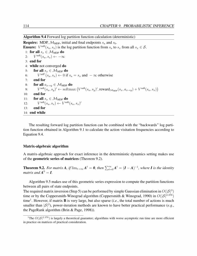
114 CHAPTER 9. PROBABILISTIC INFERENCE
Algorithm 9.4 Forward log partition function calculation (deterministic)Require: MDP,MMDP, initial and final endpoints sa and sb.Ensure: V soft(sa, sx) is the log partition function from sa to sx from all sx ∈ S.
1: for all sx ∈MMDP do2: V soft(sa, sx)← −∞3: end for4: while not converged do5: for all sx ∈MMDP do6: V soft′(sa, sx)← 0 if sa = sx and −∞ otherwise7: end for8: for all ax→y ∈MMDP do9: V soft(sa, sy)
′ ← softmax(V soft(sa, sy)
′, rewardMMDP(sx, ax→y) + V soft(sa, sx))
10: end for11: for all sx ∈MMDP do12: V soft(sa, sx)← V soft(sa, sx)
′
13: end for14: end while
The resulting forward log partition function can be combined with the “backwards” log parti-tion function obtained in Algorithm 9.1 to calculate the action visitation frequencies according toEquation 9.4.
Matrix-algebraic algorithm
A matrix-algebraic approach for exact inference in the deterministic dynamics setting makes useof the geometric series of matrices (Theorem 9.2).
Theorem 9.2. For matrix A, if limt→∞ At = 0, then∑∞
t=0 At = (I− A)−1, where I is the identitymatrix and A0 = I.
Algorithm 9.5 makes use of this geometric series expression to compute the partition functionsbetween all pairs of state endpoints.The required matrix inversion (Step 5) can be performed by simple Gaussian elimination inO(|S|3)time or by the Coppersmith-Winograd algorithm (Coppersmith & Winograd, 1990) in O(|S|2.376)time1. However, if matrix B is very large, but also sparse (i.e., the total number of actions is muchsmaller than |S|2), power-iteration methods are known to have better practical performance (e.g.,the PageRank algorithm (Brin & Page, 1998)).
1The O(|S|2.376) is largely a theoretical guarantee; algorithms with worse asymptotic run time are more efficientin practice on matrices of practical consideration.

9.1. STATISTIC-MATCHING INFERENCE 115
Algorithm 9.5 Partition function calculation via matrix inversionRequire: MDP,MMDP
Ensure: {ZA→B =∑
ζA→BerewardMMDP (ζA→B)}.
1: A← 02: for all actions aX→Y ∈MMDP do3: AX,Y ← erewardMMDP (SX)+rewardMMDP (AX→Y )
4: end for5: B← (I− A)−1 − I6: for all state pairs SA ∈MMDP and SB ∈MMDP do7: ZA→B ← BA,B
8: end for
9.1.3 Convergence Properties and ApproximationAll of the algorithms that we have presented for inference require convergence—either of the val-ues of a dynamic program (Algorithm 9.1), the steady-state visitation values (Algorithm 9.3), or thesequence of matrix multiplications (Algorithm 9.5). For finite time horizon settings, convergenceis guaranteed. However, assuming a finite horizon may be inappropriate for many application set-tings. The natural question is then: in which settings do these algorithm convergence requirementshold over infinite horizons?
Remark 9.3. The convergence properties of the maximum causal entropy model can be brokeninto three regimes:
• Strong non-convergence: the most likely policy under the model produces state-action se-quences that, in expectation, have infinite length.
• Weak non-convergence: the most likely policy produces state-action sequences that are, inexpectation, finite in length, but the expected length of all state-action sequences (averagedover all policies) is infinite in length.
• Convergence: expected state-action sequence lengths are finite when generated under themost likely policy and when averaged over all policies.
Strong non-convergence has a straight-forward parallel in deterministic planning problems:when a cycle of positive reward exists along a path between two endpoints, the optimal plan (andthe log partition function) will be undefined and its value will not converge. For stochastic state-transition dynamics, the analogy is having a subset of states where a policy that only transitionsto that subset of states yields positive expected reward from any state from that subset. Weaknon-convergence is specific to the probabilistic, softened Bellman setting, and has no optimalcontrol parallel. Due to this difference, restraints that guarantee optimal control convergence donot guarantee convergence in the maximum causal entropy model.

116 CHAPTER 9. PROBABILISTIC INFERENCE
Remark 9.4. Though strictly negative rewards ensure convergence in the state and action valuefunctions of the optimal control setting, they do not ensure convergence in the corresponding max-imum causal entropy setting (i.e., of the soft-maximum log partition functions for states and ac-tions).
Figure 9.1: An illustrative example of non-convergence with strictly negative rewards for each deterministicaction. We consider the case where each action has a cost (i.e., a negative reward) ε > 0. Note that themost likely state-action sequence is the immediate transition to from s1 to s2 (with cost ε). However, thecontribution to the partition function for paths that cycle at state s1 a total of x times is 2xe−x ε = ex ln 2−x ε.Thus, for ε ≤ ln 2, the partition function does not converge.
Figure 9.1 provides a simple example demonstrating the non-convergence of the potential func-tion in the weak non-convergence regime of behavior (Remark 9.4).
A number of structural restrictions on the state transition dynamics do ensure partition functionconvergence in general decision settings. We note three:
• Directed, acyclic decision structures: the state transition dynamics restrict the sequence ofstates and actions so that no sequence can revisit the same state. Thus, every trajectory mustterminate with finite length, guaranteeing partition function convergence.
• Finite horizon structures: finite length trajectory is considered with potentially cyclic se-quences. Explicit dependence on the time step is required by the log partition function:
Vsx→sb, t+1 = softmaxax,y
(∑sz
P(sz|ax,y, sx)Vsy→sb, t
), (9.5)
and in the corresponding time-varying policy.
• Discounted future rewards: at each timestep the state-action sequence ends with probabil-ity (1− γ) for γ > 0. The remaining outcomes dynamics are multiplicatively scaled by thediscount factor, γ.
An important convergence guarantee results from employing discounting.

9.1. STATISTIC-MATCHING INFERENCE 117
Theorem 9.5. In a discounted future rewards setting with a bounded instantaneous reward anda bounded number of actions, the partition functions of the maximum causal entropy model withfinite rewards are guaranteed to converge.
Convergence is also possible in infinite horizon, non-discounted, cyclic decision structures, butonly for some choices of parameters. For example, in the deterministic setting when the eigenval-ues of the constructed transition reward matrix (Algorithm 9.5) are less than 1.
9.1.4 Propagation Optimizations and ApproximationsFor large MDPs, Algorithms 9.4 and 9.1 may be too slow in practice to employ for computing thepartition functions for the class of all paths of a large length (T). We could just consider a smallerlength, but small length paths may represent only a small portion of the probability mass in thecomplete set of paths or fail to connect from constrained origin and terminal states. For example,under certain parameter choices, a parameterized reward Markov decision process assigns nearlyall probability mass to the optimal action choices of each state. Intuitively, approaches similarto the specialized, fast algorithms for finding optimal solutions for decision problems (e.g., A*search (Hart et al., 1968) for planning settings) should be employed for the “softened” version ofthose decision settings as well. Based on this motivation, we consider a smaller class of paths thatcontains most of the probability mass of the larger class of paths, while being significantly moreefficient to compute.
Definition 9.6. Consider some ordering, Order(S) → Z, over states of the Markov decision pro-cess. We call a path, ζ , consistent with this ordering if ∀St,St+1∈ζ Order(St) < Order(St+1). Wecall a path k-inconsistent with ordering Order if ∀St,St+1∈ζ Order(St) > Order(St+1) at most ktime.
Rather than consider all paths of length T in our inference, we will now consider all paths thatare k-consistent with an ordering.
If we have convergent partition functions, and consider a very large length T and consistencyk, the set of paths that differ between the two classes will be small and contribute only a very smallamount to the overall probability mass of log partition functions.
To help illustrate the advantages of this class of paths, consider states sa and sb in a Markovdecision process with the minimum length of paths connecting the two states being L. We will haveto consider paths of length greater than L using more than L iterations of our standard inferencealgorithm to have any estimate at all for visitation frequencies. However, if the ordering is carefullychosen, the order-consistent set of paths will contain some paths from sa to sb and provide areasonable estimate of visitation frequencies.
We can efficiently consider the log partition functions based on the k-consistent class of pathsfor some ordering by employing the dynamic program of Algorithm 9.6.
State log partition values are updated according to the ordering and, unlike the non-optimizedvariant (Algorithm 9.1), the results of the updates from earlier in the ordering are propagated

118 CHAPTER 9. PROBABILISTIC INFERENCE
Algorithm 9.6 Optimized stochastic policy calculation
Require: MDP,MMDP, state ordering, Order, and terminal state reward function, φ(s)→ R.Ensure: a maximum causal entropy policy, π(ax,y|sx).
1: for all States sx do2: Vsx ← −∞3: end for4: t← 05: while not converged do6: for all States sx according to the reverse of ordering Order do7: Vsx ← φ(sx)8: for all Actions ax,y from state sx do9: Vsx ← softmax (Vsx ,
∑Z P(sz|sx, ax,y)Vsz)
10: end for11: end for12: for all Actions ax,y do13: πt(ax,y|sx)← e(
∑z P(sz |sx,ax,y)Vsz)−Vsx
14: end for15: t← t+ 116: end while
through states later in the ordering. In the deterministic dynamics setting, with state action se-quences constrained to start in state sa and terminate in state sb, we employ a heuristic to ordereach state (si) based on the state’s fractional progress between sa and sb. Three heuristics basedon this notion of progress are:
progress1(si) =minζsa→si reward(ζsa→si)
minζsa→si reward(ζsa→si) + minζsi→sb reward(ζsi→sb); (9.6)
progress2(si) = 1−minζsi→sb reward(ζsa→si)
minζsa→si reward(ζsa→si) + minζsi→sb reward(ζsi→sb); (9.7)
progress3(si) =
{progress1(si) if minζsa→si < minζsi→sbprogress2(si) otherwise
}(9.8)
We then generate our state order based on this measure of progress using a fixed domain-dependentreward function. When there is no specific terminal state constraint, the cost of the optimal pathfrom the initial state, minζsa→si reward(ζsa→si), can be employed as an ordering criteria for thestates. Similar heuristic-based approaches can be employed in the stochastic setting by first solvinga fixed parameter optimal control problem and employing the resulting state value function to orderthe states.
The expected state and action visitation frequencies are similarly calculated according to thisoptimized reward function using Algorithm 9.7.

9.1. STATISTIC-MATCHING INFERENCE 119
Algorithm 9.7 Optimized expected state frequency calculation
Require: MDP,MMDP, time-varying policy, πt(ax,y|sx)), and an initial state distribution P0(sx).Ensure: state visitation frequencies, Dsx , under policy πt(ax,y|sx).
1: for all states sx ∈MMDP do2: Dsx ← 03: end for4: t← largest time-index of π5: while not converged do6: for all states sz according to ordering O do7: Dsz ← P0(sz)8: for all actions ax,y ∈MMDP such that Sz is a possible stochastic outcome of ax,y do9: Dsz ← Dsz +Dsx πt(ax,y|sx) P(sz|ax,y, sx)
10: end for11: end for12: t← t− 113: end while
As a second optimization, paths through states that are very far away from A and B oftencontribute little to the probability mass of the partition function. We only include states in ourordering that are within a certain threshold: minζA→i cost(ζA→i)+minζi→B cost(ζi→B) < C, wherethe threshold is determined by minζA→B cost(ζA→B). For example, C = αminζsa→si cost(ζsa→si)+ε for some α > 1 and ε > 0. Optimal state values (i.e., optimal path costs in the deterministicsetting) are again based on a fixed heuristic.
While additional optimizations for the inference algorithm are possible based on intelligentlyordering the updates, there is an important technical consideration to keep in mind: any heuristicsemployed to guide inference optimizations that depends on a learned cost weight may create non-convexity when trying to optimize for that cost weight. In other words, adapting the ordering canlead to non-convexity when fitting the parameters of a maximum causal entropy model to observeddata. This risk may be appropriately mitigated—either in theory or in practice—but we do notexplore dynamic re-orderings in this work.
9.1.5 Linear Quadratic Inference
For continuous state and continuous control inverse optimal control, the inference procedure isvery similar to Algorithm 9.1, but instead relies on the specific properties of Gaussian distributionsand quadratic reward functions to obtain closed-form expressions. As established by Theorem6.15, when the state transition dynamics follow a linear function, st+1 ∼ N(Ast + Bat,Σ) forgiven matrices A, B, and Σ, the time-varying state-action and state values are:

120 CHAPTER 9. PROBABILISTIC INFERENCE
Qsoftθ (at, st) =
[atst
]> [ B>DB A>DBB>DA A>DA
] [atst
]+
[atst
]> [ B>GA>G
]V softθ (st) = s>t (Cs,s + Q− C>a,sC
−1a,aCa,s)st + s>t (Fs + R) + const,
where C and D are recursively computed as: Ca,a = B>DB; Cs,a = C>a,s = B>DA; Cs,s =
A>DA; D = Cs,s + Q− C>C−1a,aCa,s; and G = Fs + R.
Given terminal state quadratic reward weights, φ(s) = s>Qterminals + s>R and instantaneousreward weights, Qinstant and Rinstant, Algorithm 9.8 generates time-varying quadratic state-valueand action-value parameters.
Algorithm 9.8 Linear-quadratic regulation value inference.Require: Linear-quadratic model,Mlqr, with terminal quadratic reward parameters, Qterminal and
Rterminal; and time horizon, T .Ensure: Time-varying action-value and state-value quadratic parameters: C and D; and linear
parameters: F and G.1: D0 ← Qterminal2: G0 ← Rterminal
3: for t = 1 to T do4: Ca,a ← B>Dt−1B5: Cs,a ← B>Dt−1A6: Ca,s ← Cs,a
>
7: Cs,s ← A>Dt−1A
8: Ct ←[
Ca,a Cs,a
Ca,s Cs,s
]9: Gt ← Fs + Rinstant
10: Dt ← Cs,s + Qinstant − Cs,aC−1a,aCa,s
11: Fa ← B>G12: Fs ← A>G
13: Ft ←[
FaFs
]14: end for
The state and action matrix multiplications dominate the run time of Algorithm 9.8. With naıvematrix multiplication, the run time is O(T (dim(S)3 + dim(A)3)).
The stochastic policy is then obtained from the state-action parameter, C:
π(a|s) ∝ e−[a s]>C[a s]−[a s]>F, (9.9)
which is a multi-variate Gaussian distribution.

9.2. LATENT INFORMATION INFERENCE 121
Algorithm 9.9 Linear-quadratic state and action distribution calculation.Require: Linear-quadratic model,Mlqr, stochastic policy parameter, C, and initial state, s0.Ensure: A sequence of state and action distributions, P(st) and P(at).
1: for t = 1 to T do2: Compute joint distribution P(at, st) from P(st) and π(at|st)3: Compute P(at) by marginalizing over st: P(at) =
∫st P(at, st) ∂st
4: Compute joint distribution P(st+1, at, st) from P(at, st) and P(st+1|st, at)5: Compute P(st+1) by marginalizing over at and st: P(st+1) =
∫st,at P(st+1, at, st) ∂st ∂at
6: end for
We compute the joint distribution of states and actions from the state-dependent stochasticpolicy by employing Algorithm 9.9.
Remark 9.7. The marginalized state and actions distributions are obtained from the followinglinear relationships:
P (st) ∼ N(st|µst ,Σst) (9.10)P (at|st) ∼ N(at| − C−1
a,aCa,sst, σa,a) (9.11)
P (st+1|st, at) ∼ N(st+1|A st +B at,Σdyn), (9.12)
by iteratively conditioning the Gaussian distributions and then marginalizing over previous vari-ables.
Joint distributions and marginal distributions are obtained by transforming between the stan-dard form (i.e., mean µ and variance Σ) and the canonical, quadratic form:
P(x) ∝ eη>x− 1
2x>Λx, (9.13)
which are related by: µ = Λ−1η and Σ = Λ−1. Marginalization is simpler in standard form (bytaking a sub-matrix of Σ and sub-vector of µ), while conditioning is simpler to apply in canonical,quadratic form (by addition of the precision matrix, Λ and the vector η).
9.2 Latent Information Inference
We now consider the maximum causal entropy inference problems for influence diagrams. Thisdecision framework generalizes the inverse optimal control setting by allowing latent side infor-mation variables and imperfect side information recall. As the maximum causal entropy approachis only valid when duality holds, i.e., when perfect decision recall is guaranteed, we consider in-ference within this setting.

122 CHAPTER 9. PROBABILISTIC INFERENCE
9.2.1 Perfect Recall Visitation Counts
We start by considering a stronger restriction on the influence diagram. For the special case ofperfect recall of both past decisions and past conditioning variables (Definition 7.9), reducingthe latent information inference to the inverse optimal control inference procedure is possible bymarginalizing and employing expectations.
Algorithm 9.10 MaxCausalEnt ID inference procedure for perfect recallRequire: A maximum causal entropy influence diagram with perfect recall.Ensure: Partition functions Z(Yi|par(Yi)) that are maximum causal entropy distributed.
1: for all V ∈ V do2: Associate V with argmaxYindex∈ancest(V ) index3: end for4: for i = |Y| to 1 do5: for all values (Y ′i , par(Yi)′) do6: Zi(Y
′i |par(Yi)′)← 0
7: for all Vj associated with Yi do8: for all values par(Vj)′ do9: Compute P(par(Vj)′|par(Yi)′, Y ′i )
10: end for11: Zi(Y
′i |par(Yi)′)← Zi(Y
′i |par(Yi)′) + Epar(Vj)[θ
>FVj(par(Vj))|Y ′i , par(Yi)′]12: end for13: for all values par(Yi+1)′ do14: Compute P(par(Yi+1)′|Y ′i , par(Yi)′)15: end for16: Zi(Y
′i |par(Yi)′)← Zi(Y
′i |par(Yi)′) + Epar(Yi+1)′ [Zi+1(par(Yi+1)′)|Y ′i , par(Yi)′]
17: end for18: for all par(Yi)′ do19: Zi(par(Yi)′)← softmaxYi Zi(Yi|par(Yi)′)20: end for21: end for
Algorithm 9.10 illustrates the procedure for inferring decision probabilities in this special casebased on Theorem 6.2. Essentially, the dynamics of side information are calculated by marginal-ization and the expectations of values are computed. We assume as a subroutine an algorithm forcalculating the marginal probabilities of variables conditioned on a set of fixed evidence variablesin a Bayesian network (e.g., variable elimination or belief propagation). Expectations over theunobserved uncertainty nodes that are ancestors of value variables are employed in line 11. Thisreplaces the exact evaluations, θ>F(X,Y), of Equation 6.1.

9.3. REGRET-BASED MODEL INFERENCE 123
9.2.2 Imperfect Recall Visitation Counts
In the imperfect recall inference problem with perfect recall of past actions, action distributions arerecursively inter-dependent. As a result, the backward inductive dynamic programming techniqueof Algorithm 9.10 can not be employed since P(aT |sT ) is not independent from the distributionof past actions given state sT . Instead, we rely on a fixed point iteration algorithm that iterativelyupdates the stochastic policy in hope of obtaining a fixed point solution to the inter-dependentprobability distributions.
Algorithm 9.11 MaxCausalEnt ID inference procedure for imperfect side information recallRequire: A maximum causal entropy influence diagram with perfect decision recall.Ensure: Partition functions Z(Yi|par(Yi)) that are maximum causal entropy distributed.
1: for all actions nodes, at do2: Set P(at|par(at)) to a uniform distribution3: end for4: Zpar(aT+1) = Utility(s, a)5: while not sufficiently converged do6: for τ = T to 1 do7: Compute P(anc(aτ )|par(aτ ))8: Compute P(par(aτ+1)|aτ , par(aτ ))9: for all aτ , par(aτ ) do
10: Zaτ |par(aτ ) = EP(par(aτ+1)|aτ ,par(aτ ))[Zpar(aτ+1)|aτ , par(aτ )]11: end for12: for all par(aτ ) do13: Zpar(aτ ) = softmaxaτ Zaτ |par(aτ )
14: end for15: end for16: end while
Algorithm 9.11 illustrates the procedure for obtaining the maximum causal entropy policy forthis more general imperfect information setting with perfect past decision recall.
9.3 Regret-Based Model Inference
The algorithms for considering multi-agent game settings maximize the causal entropy of the jointdistribution of players’ actions at each point in time, denoted at1:N , while enforcing rationalityconstraints.

124 CHAPTER 9. PROBABILISTIC INFERENCE
9.3.1 Correlated Equilibria InferenceAs established by Theorem 8.15, maximum causal entropy correlated equilibria are distributedaccording to Equation 9.14:
πMCECEλ (at1:N |st) ∝ e
−(∑
i,ati′ λi,st,ati,a
ti′ ExpectDevGain
πMCECEλi (at1:N ,st,ati
′))
+ExpectEntλ(at1:N ,st), (9.14)
where ExpectEnt(at1:N , st) , Eat+1
1:N ,st+1
[ExpectEntλ(a
t+11:N , s
t+1) +H(at+11:N |st+1)
∣∣at1:N , st]. The
free parameters, λ, are chosen to maximize the causal entropy while enforcing deviation regretconstraints for the joint action distribution of each state.
The naıve approach to this problem is to jointly maximum the entropy of the optimization tofind all λ parameters for each time step and state in parallel, as shown in Algorithm 9.12.
Algorithm 9.12 MCECE strategy profile computation for finite horizonRequire: A fully-specified Markov game.Ensure: A maximum causal entropy correlated equilibrium.
1: λ(1) = {λ(1)
t,i,st,ati,ati′} ← (arbitrary) positive initial values.
2: x← 13: while not converged do4: Compute π(x)
λ = {πλ(at1:N |st)} from λ(x) using a subroutine.5: Take an optimization step using π(x)
λ to improve λ(x+1)
6: x← x+ 17: end while
However, the Markovian relationship between variables can be exploited to improve the opti-mization procedure.
Remark 9.8. For time-varying policies, future strategy probabilities (and dual parameters) are in-dependent of earlier strategy and dual parameters given the state. As a result, a sequence dynamicprogramming approach can be employed to compute the maximum causal entropy equilibrium.
Following Remark 9.8, Algorithm 9.12 can be re-expressed as a sequential dynamic program-ming algorithm (Algorithm 9.13) resembling value iteration (Bellman, 1957). It iteratively com-putes both future expected utilities and expected entropies by fully optimizing λ parameters attimestep T and then employing the corresponding expected utilities and expected entropies for theoptimization at timestep T − 1. This process is iteratively continued to obtain the policy for alltimesteps.
We investigate algorithms for the optimization problem of Step 4 of Algorithm 9.13 in Chapter10.

9.4. DISCUSSION 125
Algorithm 9.13 Value iteration approach for obtaining MCECERequire: A fully-specified Markov game.Ensure: A maximum causal entropy correlated equilibrium.
1: ∀i,a1:N ,s ExpectUtili(a1:N , s)← Utilityi(a1:N , s)2: ∀a1:N ,s ExpectEnt(a1:N , s)← 03: for t = T to 1 do4: For each state, st, obtain {πλ(at1:N |st)} using ExpectUtil and ExpectEnt values in the fol-
lowing optimization:
argmaxπ(at1:N |st)
H(at1:N |st) + Eπ(at1:N |st)[ExpectEnt(a1:N , s)|st
]such that:
∑a−i
P(at1:N |st)(ExpectRegret({at−i, ati}, st)− ExpectRegret(at1:N , s
t))≤ 0
∀at1:N P(at1:N |st) ≥ 0 and∑at1:N
P(at1:N |st) = 1.
5: ∀i,a1:N ,s ExpectUtil′i(a1:N , s)← γ∑
at1:N ,st π(at1:N |st) P(st|s, a1:N) ExpectUtili(a
t1:N , s
t)
6: ∀s,a1:N ExpectEnt′(a1:N , s) ← γ∑
at1:N ,st π(at1:N |st) P(st|s, a1:N)
(ExpectEnt(at1:N , s
t) +
H(at1:N |st))
7: ∀i,a1:N ,s ExpectUtili(a1:N , s)← ExpectUtil′i(a1:N , s) + Utilityi(a1:N , s)8: ∀a1:N ,s ExpectEnt(a1:N , s)← ExpectEnt′(a1:N , s)9: end for
9.4 DiscussionIn this chapter, we have presented algorithms for efficient inference within the maximum causal en-tropy framework. For equality-constrained maximum causal entropy, the inference algorithms aresoftened extensions of value iteration dynamic programming procedures. With inequality-basedrationality constraints, a similar dynamic programming procedure is employed to propagate infor-mation backwards over time. However, a convex optimization is required to obtain the maximumcausal entropy policy at each state and timestep.
The efficiency provided by these algorithms is important. Rather than reasoning depending onan entire history, which grows exponentially with history length, reasoning is generally linear inthe history size, as long as the dynamics governing side information are Markovian. This efficiencyenables the maximum causal entropy approach to be applied to large decision prediction tasks inPart IV of the thesis.

Chapter 10
Parameter Learning
“Our knowledge is a little island in a great ocean of non-knowledge.”— Isaac Singer (Inventor, 1811–1875).
Accurately predicting future behavior based on previously observed behavior sequences re-quires fitting the parameters of the maximum causal entropy probability distribution using that ob-served training data. Since no closed-form solution exists for the best parameter choice in general,maximum entropy optimization-based approaches must instead be employed to obtain parametersthat provide accurate prediction. In this chapter, we describe the maximum causal entropy gradi-ents and the gradient-based optimization methods that we employ to learn model parameters fromtraining data. In the case of rationality requirements for behavior in sequential games, optimiza-tions techniques are required to enforce the rationality constraints independently of observed gameplay.
10.1 Maximum Causal Entropy Model Gradients
By employing the Lagrangian of the maximum causal entropy optimization (Definition 5.6) andsolving for the causally conditioned probability distribution form, we are left to only enforce the re-maining constraints—either purposeful equality constraints or inequality constraints guaranteeingrationality.
10.1.1 Statistic-Matching Gradients
In the statistic-matching maximum causal entropy model (Chapter 6), the gradient of the dual isthe difference between empirical feature counts and expected feature counts:
126

10.1. MAXIMUM CAUSAL ENTROPY MODEL GRADIENTS 127
∇θ Fdual(θ) =
(EP(X,Y)
[∑t
F (xt, yt)
]− EP(X,Y)
[∑t
F (xt, yt)
]). (10.1)
We employ Algorithm 10.1 to compute the expected feature sum under the maximum causalentropy model’s policy (obtained via Algorithm 9.1). The empirical feature counts can be triviallyobtained by calculating the empirical visitation frequency and weighting each state’s feature bythis count.
Algorithm 10.1 Feature expectation calculation
Require: MDPMMDP, initial state s0, stochastic policy, π(a|s).Ensure: Expected feature counts, E[f], under the stochastic policy, π(a|s).
1: Compute Dsx under π(a|s) from state s0 using Algorithm 9.72: E[f]← 03: for all sx ∈MMDP do4: for all ai from state sx do5: E[f]← E[f] +Dsx π(ai|sx) fsx,ai6: end for7: end for
In the linear-quadratic regulation setting, expected sums of quadratic states and actions serveas continuous analogs to the feature function sums of the discrete state and action setting. Themaximum causal entropy dual’s gradient in this setting is simply the difference between thesesums of quadratics or linear state functions under the empirical distribution and under the model’sexpectation, as shown in Equation 10.2 and Equation 10.3:
∂Fdual(θ)
∂Q=
(EP(s1:T ,a1:T )
[∑t
st s>t
]− EP(s1:T ,a1:T )
[∑t
st s>t
]); (10.2)
∂Fdual(θ)
∂R=
(EP(s1:T ,a1:T )
[∑t
st
]− EP(s1:T ,a1:T )
[∑t
st
]). (10.3)
Employing the inferred state and action distributions at each point in time (Algorithm 9.9), thequadratic expectations of states and actions are calculated according to Algorithm 10.2.
The integrals of Algorithm 10.2 are computed using the following Gaussian property:Ex∼N(µ,Σ)[x x>] = µµ> + Σ.

128 CHAPTER 10. PARAMETER LEARNING
Algorithm 10.2 Quadratic expectation calculation
Require: LQRMLQR, state distribution P(st), action distribution P(at).Ensure: Expectations, E[
∑t st s>t ] and E[
∑t at a>t ] based on distributions P(st) and P(at).
1: E[∑
s s>]← 02: E[
∑a a>]← 0
3: for t = 1 to T do4: E[
∑s s>]← E[
∑s s>] +
∫st P(st) st s>t ∂st
5: E[∑
a a>]← E[∑
a a>] +∫
at P(at) at a>t ∂at6: end for
10.1.2 Latent Information Gradients
The gradients for the latent information setting (Chapter 7) are very similar to those of the previ-ous subsection; they are also differences between empirical feature expectation sums and featureexpectations under the maximum causal influence diagram model.
Algorithm 10.3 MaxCausalEnt ID Gradient CalculationRequire: A maximum causal entropy influence diagram and initial parameters, θ.Ensure: log gradient,∇θ logP (y||par(y))
1: Compute E[F ]← 1T
∑t EX,Y[
∑V F(V )|xt, yt]
2: Compute Z(par(Y )), Z(Y |par(Y )) via Algorithm 9.10 for Parameters θ3: for all decision nodes Yi do4: Replace Yi with an uncertainty node with probabilities P(yi|par(Yi)) = eZ(yi|par(Yi))−Z(par(Yi))
5: end for6: E[F ]← Ok
7: for all V do8: for all values par(V )′ do9: Compute P(par(V )′) using {P(yi|par(Yi))}
10: end for11: E[F ]← E[F ] + E[F (V )]12: end for13: ∇θ log P(y||par(y))← E[F ]− E[F ]
The added expectation in the maximum causal entropy influence diagram setting preserves theconvexity of the optimization since the feature matching constraint remains linear in the causallyconditioned probabilities. Standard gradient-based optimization techniques can be employed usingthe gradient calculated in Algorithm 10.3.

10.2. CONVEX OPTIMIZATION METHODS 129
10.1.3 Maximum Causal Entropy Correlated Equilibrium GradientsIn the maximum causal entropy correlated equilibrium setting, optimization of model parametersis also required. In this case, optimization is not employed to match empirical statistics of observeddata, but instead to enforce the remaining deviation regret constraints.
From Theorem 8.15 we have the form of the maximum causal entropy correlated equilibriumdistribution:
πMCECEλ (at1:N |st) ∝ e
−(∑
i,ati′ λi,st,ati,a
ti′ ExpectDevGainπ
MCECEi (at1:N ,st,ati
′))
+ExpectEnt(at1:N ,st), (10.4)
where ExpectEnt(at1:N , st) , Eat+1
1:N ,st+1
[ExpectEnt(at+1
1:N , st+1) +H(at+1
1:N |st+1)∣∣at1:N , s
t].
The gradient of the log strategy distribution is thus:
∂
∂λi,st,ati,ati′log πMCECE
λ (at1:N |st) =(P(at1:N |st)− 1
)ExpectDevGainπi (at1:N , s
t, ati′) (10.5)
∂
∂λi,st,ati,ati′log πMCECE
λ (at1:N |st) =(P(at1:N |st)
)ExpectDevGainπi (at1:N , s
t, ati′), (10.6)
when each deviation regret constraint is violated (i.e., λ > 0).
10.2 Convex Optimization MethodsUsing the gradient presented in Section 10.1 for each of the maximum causal entropy models, weemploy standard gradient-based optimization techniques to fit model parameters from data.
10.2.1 Gradient DescentThe standard, simple gradient-based optimization method is gradient ascent. It iteratively takessteps in the direction of the gradient to improve the model parameters according to varying stepsizes.
Algorithm 10.4 illustrates the procedure for following the gradient towards the function’s op-timal point. Standard gradient ascent is often impractically slow for many optimization problems.One standard technique is to replace the decaying step size with line search, that finds the optimalstep size by performing a binary search along the line in the direction of the gradient.
10.2.2 Stochastic Exponentiated GradientWhen the gradient is computationally expensive to obtain for each training example, computing theentire gradient before taking an optimization step can be extremely slow. Instead, stochastic opti-mization (Robbins & Monro, 1951) can be employed to take optimization steps after the gradient

130 CHAPTER 10. PARAMETER LEARNING
Algorithm 10.4 Gradient Ascent calculation
Require: Gradient function∇θF (a, s)→ R|θ|, training data {a(i), s(i)}, and learning rate λ.Ensure: Approximately optimal θ parameters.
1: ∇F ← 02: Initialize θ to random initial values3: t← 10004: while not sufficiently converged do5: for all i do6: ∇F ← ∇F +∇θF (a(i), s(i))7: end for8: θ ← θ − λ
t∇F
9: t← t+ 110: end while
for each example or small groups of examples are calculated. The empirical improvements of thestochastic approach have been demonstrated in maximum entropy-based models (Vishwanathanet al., 2006) and other large-scale machine learning tasks. We combine this with the idea of tak-ing exponentiated gradient steps (Kivinen & Warmuth, 1997). This exponentiation techniques hasbeen shown to provide better convergence rates than standard linear gradient update methods.
Algorithm 10.5 Stochastic exponentiated gradient ascent calculation
Require: Gradient function∇θF (a, s)→ R|θ|, training data {a(i), s(i)}, and learning rate λ.Ensure: Approximately optimal θ parameters.
1: Initialize θ to random initial values2: t← 10003: while not sufficiently converged do4: for all i in random order do5: θ ← θe−
λt∇θF (a(i),s(i))
6: t← t+ 17: end for8: end while
Algorithm 10.5 illustrates the small differences from gradient ascent that allow stochastic (i.e.,online) optimization of the objective function. Often small batches of examples (rather than sin-gle examples) are employed to more robustly obtain the gradient step direction of Step 5 of thealgorithm.

10.2. CONVEX OPTIMIZATION METHODS 131
10.2.3 Subgradient MethodsWhen the function being optimized is not smooth, but still convex, sub-gradient methods can beemployed to obtain the optimal parameters. For inequality-constrained optimizations, an alterna-tive to taking optimization steps based on the gradient using the entire set of remaining distributionconstraints is to individually apply each violated constraint or a small set of violated constraintsusing the sub-gradient algorithm. This is particularly useful for enforcing inequality constraints.
Given a convex optimization problem of the form:
minθf(θ)
such that: ∀i hi(θ) ≤ 0,
the corresponding feasibility optimization can be re-written as an unconstrained optimization (Boydet al., 2003):
minθ
maxihi(θ). (10.7)
The method of subgradient optimization (Shor et al., 1985) can then be applied.
Algorithm 10.6 Sequential constraint, sub-gradient optimization
Require: Inequality constraint functions {h}, inequality constraint gradient {∇h}, and objectivegradient,∇f , initial parameters, θ.
Ensure: Feasible, near-optimal solution to the convex optimization.1: t← 10002: while not sufficiently converged or not feasible do3: if a violated constraint exists then4: i← most violated constraint5: ∇F ← ∇θ hi(θ)|θ6: else7: ∇F ← ∇θ f(θ)|θ8: end if9: θ ← θ − λ
t∇F
10: t← t+ 111: end while
The subgradient optimization of Algorithm 10.6 extends the feasibility optimization of Equa-tion 10.7 to include an objective function. It sequentially finds a violated constraint and takesoptimization steps to satisfy that constraint. This process continues until a feasible point is found,at which point an optimization step that improves upon the objective function is taken. We employthis technique to enforce rational inequality constraints in the multi-player game setting.

132 CHAPTER 10. PARAMETER LEARNING
10.2.4 Other Convex Optimization MethodsA number of more sophisticated methods for convex optimization exist that either employ theHessian of the objective function, or approximate the Hessian to improve optimization efficiency.Describing each of these methods is beyond the scope of this work. Instead, we treat them as blackboxes. The BFGS algorithm (Broyden, 1970; Fletcher, 1970; Goldfarb, 1970; Shanno, 1970) isone such technique based on Newton’s method of optimization. Interior point methods (Nesterov& Nemirovski, 1987) are also applicable for inequality-constrained optimizations.
These techniques provide better theoretical convergence guarantees than the simpler optimiza-tion techniques previously described. However, we employ the simpler methods in practice.
10.3 Considerations for Infinite HorizonsWhen considering decision problems with infinite horizons, it is often possible for the inferencealgorithm to be non-convergent for particular values of parameters (as discussed in Section 9.1.3).This complicates simple gradient-based optimization approaches. We present the following threetechniques to address this complication.
10.3.1 Projection into Convergent RegionIn some settings, constraints on the parameters that enforce convergence can be established. Forinstance, in the LQR setting, if the Q matrix is positive-definite, then convergence of the D matrixover infinite horizons (but ultimately terminating with fixed variance) is guaranteed. This positivedefinite requirement can be enforced by projecting the Q matrix using its eigenvalue decompositionand making its negative eigenvalues ε.
Convergence-Preserving Gradient Steps
A very similar option is to employ gradient steps that ensure convergent inference. This is difficultin general, but possible for some special cases. For example, exponentiated matrix gradient algo-rithms (Tsuda et al., 2006) take gradient steps that preserve positive-definiteness. The update stepis as follows, for learning rate λ:
Q← elog Q−λQ∇. (10.8)
Here the exponentiation and logarithm operators are matrix operations rather than scalar operators.
10.3.2 Fixed Finite Decision StructuresA second technique to address the infinite horizon and non-convergent inference considerations isto approximate with a fixed horizon, as discussed in Section 9.1.3, or to employ other convergent

10.4. DISCUSSION 133
inference guaranteeing constraints on the structure of the sequential decision representation. Forexample, employing discounting naturally forces inference to converge.
10.3.3 Optimization Line-Search and BacktrackingA third technique is to leverage optimization algorithms that employ line search or provide back-tracking. Choosing initial parameters that guarantee convergence (i.e., those with very high cost,or large negative reward) is often straight-forward. Gradient-based optimization algorithms thatsearch along the gradient to find the optimal (convergent) point or detect non-convergent inferenceare then employed. As an example of the latter, in standard gradient-ascent, when a parameteroptimization step is taken that leads to non-convergent inference, the algorithm reverts to the lastconvergent inference parameters and the learning rate is decreased.
10.4 DiscussionIn this chapter, we have presented optimization techniques for fitting parameters of the maximumcausal entropy models from observed data. The algorithms required for learning are simple appli-cations of common convex optimization techniques. We view this as an advantage; no specializedoptimization methods are required and, due to convexity, good optimization convergence guar-antees exist. In practice, these simple techniques perform well for training the maximum causalentropy models of this thesis.

Chapter 11
Bayesian Inference with Latent Goals
“People’s behavior makes sense if you think about it in terms of their goals, needs, and motives.”— Thomas Mann (Novelist, 1875–1955).
Up until this point of the thesis we have considered the problem setting where intentions—inthe form of terminal state constraints on behavior sequence within our maximum causal entropyframework (i.e., terminal utility φ from Algorithm 9.1 described in Section 9.1.1)—have beenknown or assumed. In many problem settings, these intentions, or goals, are not known a prioriand inferring them given only the partial demonstration of a sequences of states and actions drivesa number of important applications. In this chapter, we investigate methods for Bayesian inferenceof goals and remaining trajectories to unknown goals. Additionally, we provide algorithms withsignificant efficiency improvements for the setting with deterministic state dynamics.
11.1 Latent Goal Inference
Latent goal inference is the task of predicting the end target, or goal, of a partial sequence ofbehavior. More formally, a partial sequence of states and actions, {s1:t, a1:t}, is provided. Byassumption, when complete, the full sequence will terminate in one state from a set of possiblegoal states, G ∈ G ⊆ S. The probabilistic goal inference problem is to provide a distribution overthe possible goal locations.
11.1.1 Goal Inference Approaches
Goal inference can be framed as a probabilistic classification task mapping from the partial tra-jectory, {s1:t, a1:t} to a probability distribution over possible goals, P (G). A maximum entropyapproach to this problem would define features between the goal variable and partial trajectory
134

11.1. LATENT GOAL INFERENCE 135
variables, F({s1:t, a1:t}, G). The conditional probability of a goal is then:
P (G|s1:t, a1:t) ∝ eθ>F({s1:t,a1:t},G) (11.1)
This prediction technique provides the worst-case log-loss guarantees of maximum entropy. How-ever, a difficulty of this approach is constructing good features that are a function of the goal stateand the partial behavior sequence. For large decision tasks, natural choices of features (i.e., thequadratic interaction terms of partial trajectory states and goal states) can be quite large. Thismakes fitting the predictive model from a limited amount of observed behavior sequences difficult.
11.1.2 Bayesian Formulation
An alternate approach avoids the potential difficulties of defining a compact set of features relatinggoals and partial behavior sequences. Using a goal-conditioned distribution as a probabilistic pol-icy, Bayes’ rule can be employed to update a belief in which of those goal states the sequence willultimately terminate. The initial belief is expressed as a prior distribution, P(G), and the posteriordistribution is then:
P(G|s1:t, a1:t) =P(a1:t|s1:t, G) P(G)∑G′ P(a1:t|s1:t, G′) P(G′)
(11.2)
∝
[∏t
πG(at|st, G)
]P(G),
where πG(at|st) denotes the policy that is constrained to goal state G.The computational complexity of obtaining this posterior is largely dependent on the complex-
ity of computing each action’s conditional probability and the amount of computational re-usepossible when calculating conditional probabilities and related quantities.
The naıve approach to latent goal inference computes the posterior probability directly accord-ing to Equation 11.2. Algorithm 11.1 illustrates the steps required.
The main bottleneck of this algorithm is that a maximum causal entropy policy must be calcu-lated for each goal state in the goal set. This yields O(|G|) total policy inference executions (Algo-rithm 9.1), which dominates the algorithm’s run time for a total ofO(|G|T |S||A|) orO(|G|T (|S|+|A|)) depending on the sparsity of the stochastic transition dynamics (and where T is the numberof iterations of the inference algorithm).
11.1.3 Deterministic Dynamics Simplification
In the special case of domains with exclusively deterministic dynamics, we exploit the reversibilityof computing the log partition functions to obtain a more efficient algorithm.

136 CHAPTER 11. BAYESIAN INFERENCE WITH LATENT GOALS
Algorithm 11.1 Naıve latent goal inference
Require: MDPMMDP, trajectory a1:t, s1:t, set of goals G = {G}, prior distribution P(G).Ensure: {P(G|a1:t, s1:t)} posterior distributed according to Equation 11.2.
1: Z ← 02: for all G ∈ G do3: Compute πG(a|s) using Algorithm 9.14: P(G|a1:t, s1:t)← 15: for all τ = 1 to t do6: P(G|a1:t, s1:t)← P(G|a1:t, s1:t) πG(aτ |sτ )7: end for8: Z ← Z + P(G|a1:t, s1:t)9: end for
10: for all G ∈ G do11: P(G|a1:t, s1:t)← P(G|a1:t,s1:t)
Z
12: end for
Theorem 11.1. The posterior distribution of goals can be obtained from the log partition functions,Vsx→sy , as follows:
P(G|a1:t, s1:t) ∝ P(G) eVst→G − Vs1→G . (11.3)
The difference in log partition functions, Vst→G−Vs1→G, can be interpreted as the progress thatthe partial sequence has made towards potential goal state, G. Goal state likelihood is maximizedby the choice of goal towards which the most progress has been made.
Algorithm 11.2 employs the result of Theorem 11.1 to compute the posterior goal distributionfrom log partition functions.
Algorithm 11.2 Efficient latent goal inference for deterministic dynamics
Require: MDPMMDP, trajectory a1:t, s1:t, set of goals G = {G}, prior distribution P(G).Ensure: P(G|a1:t, s1:t) posterior distributed according to Equation 11.2.
1: Compute Vs1→sx for all sx via the forward updates of Algorithm 9.4.2: Compute Vst→sx for all sx via the forward updates of Algorithm 9.4.3: for all G ∈ G do4: P(G|a1:t, s1:t)← P(G) eVst→G−Vs1→G
5: Z ← Z + P(G|a1:t, s1:t)6: end for7: for all G ∈ G do8: P(G|a1:t, s1:t)← P(G|a1:t,s1:t)
Z
9: end for

11.2. TRAJECTORY INFERENCE WITH LATENT GOAL STATE 137
Compared to Algorithm 11.1, this approach reduces the required number of policy inferencesfrom O(|G|) to O(1). This provides a total run time of O(T (|S| + |A|)). In many settings, thisO(|G|) reduction makes latent goal inference practical for large decision problems.
11.2 Trajectory Inference with Latent Goal StateA related important prediction task is that of inferring a future sequence of state and actions whenthe goal state is unknown and an initial trajectory, a1:t and s1:t, has been observed. These tasksbuild upon the latent goal state inference task by adding trajectory prediction given an inferredgoal state distribution.
11.2.1 Bayesian FormulationAny probabilistic goal inference technique can be employed. However, we will consider theBayesian latent goal inference perspective. We focus specifically on the problem of calculatingthe estimated occurrences of some state Sx under the maximum causal entropy distribution withlatent goal state:
Dsx|s1:t,a1:t , EP(st+1:T ,at+1:T |s1:t,a1:t)
[T∑
τ=t+1
I(sx = sτ )
∣∣∣∣∣s1:t, a1:t
]. (11.4)
Other related inferences, such as calculating the probability of a continuation trajectory or sub-trajectory can be realized with small modifications.
A simple approach to this inference task is to expand the definition of the expected state visita-tions (Equation 11.4) and re-expresses it in terms of the latent goal state, G:
Dsx|s1:t,a1:t =∑
st+1:T ,at+1:T
(T∑
τ=t+1
I(sx = sτ )
)P(at+1:T , st+1:T |a1:t, s1:t) (11.5)
=∑G
∑st+1:T ,at+1:T
(T∑
τ=t+1
I(sx = sτ )
)P(st+1:T , at+1:t|at, st, G) P(G|s1:t, a1:t)
=∑G
∑st+1:T ,at+1:T
(T∑
τ=t+1
I(sx = sτ )
)P(st+1:T , at+1:t|at, st, G)
P(s1:t, a1:t|G) P(G)∑G′ P(s1:t, a1:t|G′) P(G′)
The naıve algorithm for latent trajectory inference computes the values of this expansion di-rectly, as shown in Algorithm 11.3.
The total run time is again either O(|G|T |S||A|) or O(|G|T (|S| + |A|)) depending on thesparsity of the stochastic transition dynamics.

138 CHAPTER 11. BAYESIAN INFERENCE WITH LATENT GOALS
Algorithm 11.3 Naıve latent trajectory inference
Require: MDP MMDP, trajectory a1:t, s1:t, set of goals G = {G}, prior distribution P(G), andstate sx.
Ensure: Dsx|s1:t,a1:t computed according to Equation 11.4.1: Dsx|s1:t,a1:t ← 02: for all G ∈ G do3: Compute πG(a|s) using Algorithm 9.64: Compute P(G|a1:t, s1:t) according to Algorithm 11.15: Compute Dsx,G under πG(a|s) using Algorithm 9.36: Dsx|s1:t,a1:t ← Dsx|s1:t,a1:t +Dsx,G P(G|a1:t, s1:t)7: end for
11.2.2 Deterministic Dynamics SimplificationAs in the latent goal inference task, improved efficiency for the latent trajectory inference task canbe realized in the special case of deterministic dynamics.
Theorem 11.2. Action visitation calculations using final reward values are as follows:
φ(G) = logP (G|a1:t, s1:t)
= Vst→G − Vs1→G + log P(G),
and are equivalent to the goal-probability-weighted visitation calculations:
Dsx|s1:t,a1:t =∑
st+1:T ,at+1:T
(T∑
τ=t+1
I(sx = sτ )
)P(at+1:T , st+1:T |a1:t, s1:t)
of Equation 11.4.
Algorithm 11.4 leverages the property of Theorem 11.2 to efficiently calculate state visitationfrequencies.
The algorithm requires only one additional inference compared with latent goal inference (Al-gorithm 11.2), maintaining its overall O(1) inferences and total run time of O(T (|S|+ |A|)).
11.3 DiscussionIn this chapter, we have extended the inference procedure for maximum causal entropy to settingswhere behavior is goal-constrained, but the goal is unknown to the behavior forecaster and must beinferred. Our efficient optimizations for the deterministic dynamics setting generalizes the linearcompositionality of Todorov (Todorov, 2009a) to a full Bayesian treatment.

11.3. DISCUSSION 139
Algorithm 11.4 Efficient latent trajectory inference for deterministic dynamics
Require: MDP MMDP, trajectory a1:t, s1:t, set of goals G = {G}, prior distribution P(G), andstate sx.
Ensure: Dsx|s1:t,a1:t computed according to Equation 11.41: Compute Vst→sx for all sx via the forward updates of Algorithm 9.4.2: Compute {P(G|a1:t, s1:t)} via Algorithm 11.23: for all G ∈ G do4: φ(G)← Vst→G − Vs1→G + log P(G|a1:t, s1:t)5: end for6: Compute π(a|s) for final reward φ(s) using Algorithm 9.17: Compute Dsx using Algorithm 9.3, policy π(a|s), and initial state st
This problem was previously addressed by Baker et al. (2007) under the Boltzmann actionvalue distribution of Section 3.2.5. There are major negative computational efficiency implicationsfor employing that model for goal inference—action values must be computed for each action to allpossible goal locations. In contrast, the optimization technique of this chapter for deterministic dy-namics requires only a constant number of softmax inferences to obtain posterior goal distributionsand posterior trajectories with unknown goal.

Part IV
Applications
140

141
Overview of Part IVPart IV of the thesis employs the models of Part II and the algorithms of Part III to behaviormodeling and prediction tasks. We demonstrate that many of the theoretical niceties of the maxi-mum causal entropy framework translate into predictive and task performance improvements overexisting methods. Additionally, we show that the algorithms enable these prediction tasks to beperformed efficiently.
Chapter 12 applies maximum causal entropy inverse optimal control model to the task of assist-ing a vehicle’s driver by predicting the driver’s intended future route in a road network with roadcharacteristics available. We train a maximum causal entropy model using demonstrated globalpositioning sensor data and evaluate the predictive capabilities.
Chapter 13 applies the maximum causal entropy inverse optimal control model to the task ofcreating more intelligent robot navigation behavior. Our approach predicts future human move-ment trajectories and plans robot movements that are more complementary to those predictions.
Lastly, Chapter 14 demonstrates the wider range of applicability of the maximum causal en-tropy approach on synthetic problems in a multi-player Markov game setting, for predicting be-havior in a partial information diagnostic setting, and for predicting the controls of a device in acontinuous state and action setting.

Chapter 12
Driver Route Preference Modeling
“Americans will put up with anything provided it doesn’t block traffic.”— Dan Rather (Journalist, 1931–).
A common decision task solved by many individuals on a daily basis is that of selecting a driv-ing route to travel from point a to point b in a road network. Many different factors influence thisdecision task. They range from personal preferences to contextual factors. Global positioning sys-tem (GPS) technology allows these decision sequences to be passively observed with no additionalinteraction burden placed upon the driver. This presents opportunities for:
• Training and evaluating context-dependent decision prediction methods on large-scale se-quential decision problems.
• Creating useful applications that benefit drivers based on the ability to accurately predictdriver intentions and future behavior.
In this chapter, we apply the maximum causal entropy framework to the problem of modelingdriving route preferences and compare with other methods.
12.1 MotivationsDirectly communicating our intentions and preferences to a computational system while drivingis a difficult (and dangerous) task (Steinfeld et al., 1996). However, a computational system thatis aware of that information could be extremely valuable. For example, a navigation applicationmay be able to warn of unexpected accidents or provide more geographically relevant coffee shoprecommendations if it knew where a driver were going. Instead of relying on drivers to commu-nicate their intentions, which they often will not or cannot do, we take the opposite perspective;the navigation system itself should learn to predict the intentions and future behaviors of the driverbased on past observations and the current situation.
142

12.2. UNDERSTANDING ROUTE PREFERENCES 143
12.2 Understanding Route PreferencesPrevious research on predicting the route preferences of drivers found that only 35% of the 2,517routes taken by 102 different drivers were the “fastest” route, as defined by a popular commercialroute planning application (Letchner et al., 2006). Disagreements between route planning softwareand empirical routes were attributed to contextual factors, like the time of day, and differences inpersonal preferences between drivers.
We conducted a survey of 21 college students who drive regularly in the Pittsburgh area tohelp understand the variability of route preference as well as the personal and contextual factorsthat influence route choice. We presented each participant with four different maps labeled witha familiar start and destination point. In each map we labeled a number of different potentiallypreferable routes. Participants selected their preferred route from the set of provided routes under6 different contextual situations for each endpoint pair. The contextual situations we consideredwere: early weekday morning, morning rush hour, noon on Saturday, evening rush hour, immedi-ately after snow fall, and at night.
Table 12.1: Context-dependent route preference survey results for one pair of endpoints
RouteContext A B C D E F G
Early morning 6 6 4 1 2 2 0Morning rush hour 8 4 5 0 1 2 1
Saturday noon 7 5 4 0 1 2 2Evening rush hour 8 4 5 0 0 3 1
After snow 7 4 4 3 2 1 0Midnight 6 4 4 2 1 4 0
The routing problem most familiar to our participants had the most variance of preference. Thenumber of participants who most preferred each route under each of the contextual situations forthis particular routing problem is shown in Table 12.1. Of the 7 available routes to choose from(A-G) under 6 different contexts, the route with highest agreement was only preferred by 8 people(38%). In addition to route choice being dependent on personal preferences, route choice was oftencontext-dependent. Of the 21 participants, only 6 had route choices that were context-invariant. 11participants used two different routes depending on the context, and 4 participants employed threedifferent context-dependent routes.
Our participants were not the only ones in disagreement over the best route for this partic-ular endpoint pair. We generated route recommendations from four major commercial mappingand direction services for the same endpoints to compare against. The resulting route recommen-dations also demonstrated significant variation, though all services are context- and preference-independent. Google Maps (Google 2008) and Microsoft’s MapPoint (MapPoint 2008) both chose

144 CHAPTER 12. DRIVER ROUTE PREFERENCE MODELING
route E, while MapQuest (MapQuest 2008) generated route D, and Yahoo! Maps (Yahoo 2008)provided route A.
Participants additionally provided their preference towards different driving situations on a five-point Likert scale (see Table 12.2). The scale was defined as: (1) very strong dislike, avoid at allcosts; (2) dislike, sometimes avoid; (3) don’t care, doesn’t affect route choice; (4) like, sometimesprefer; (5) very strong like, always prefer.
Table 12.2: Situational preference survey results
PreferenceSituation 1 2 3 4 5
Interstate/highway 0 0 3 14 4Excess of speed limit 1 4 5 10 1
Exploring unfamiliar area 1 8 4 7 1Stuck behind slow driver 8 10 3 0 0
Longer routes with no stops 0 4 3 13 1
While some situations, like driving on the interstate are disliked by no one and being stuckbehind a slow driver are preferred by no one, other situations have a wide range of preferencewith only a small number of people expressing indifference. For example, the number of driverswho prefer routes that explore unfamiliar areas is roughly the same as the number of drivers withthe opposite preference, and while the majority prefer to drive in excess of the speed limit andtake longer routes with no stops, there were a number of others with differing preferences. Weexpect that a population covering all ranges of age and driving ability will possess an even largerpreference variance than the more homogeneous participants in our surveys.
The results of our formative research strongly suggest that drivers’ choices of routes varygreatly and are highly dependent on personal preferences and contextual factors.
12.3 PROCAB: Context-Aware Behavior ModelingThe variability of route preference from person to person and from situation to situation makesperfectly predicting every route choice for a group of drivers extremely difficult. We adopt themore modest goal of developing a probabilistic model that assigns as much probability as possibleto the routes the drivers prefer. Some of the variability from personal preference and situationis explained by incorporating contextual variables within our probabilistic model. The remainingvariability in the probabilistic model stems from influences on route choices that are unobservedby our model.
Many different assumptions and frameworks can be employed to probabilistically model therelationships between contextual variables and sequences of actions. The probabilistic reasoning

12.3. PROCAB: CONTEXT-AWARE BEHAVIOR MODELING 145
from observed context-aware behavior (PROCAB) approach that we employ is based on threeprincipled techniques previously introduced in this thesis:
• Representing driving route decisions as sequential actions in a parametric-reward Markovdecision process (PRMDP) with parametric costs (Definition 2.10).
• Using inverse optimal control (Section 3.2.1) to recover cost weights for the PRMDP thatexplain observed behavior.
• Employing the principle of maximum entropy (Section 5.1) and its causal extension (Sec-tion 5.2) to find the unique set of cost weights that have the least commitment.
The resulting probabilistic model of behavior is context-dependent, compact, and efficient tolearn and reason about. It can be viewed as a special deterministic case of the maximum causalentropy approach to inverse optimal control. In this section, we describe the formulation of theroute selection task as a Markov decision process. We then explain how the resulting model isemployed to efficiently reason about context-dependent behavior.
12.3.1 Representing Routes Using a Markov Decision ProcessMarkov decision processes (MDPs) (Puterman, 1994) provide a natural framework for representingsequential decision making tasks, such as route planning. The agent takes a sequence of actions(a ∈ A), which transition the agent between states (s ∈ S) and incur an action-based cost1 (c(a) ∈R). We employ the PRMDP variant where costs of actions are parameterized (Definition 2.10).A simple deterministic PRMDP with 8 states and 20 actions representing a small grid-like roadnetwork is shown in Figure 12.1.
Figure 12.1: A simple Markov Decision Process with action costs.
In the optimal control problem, the agent is trying to minimize the sum of costs while reachingsome destination. We call the sequence of actions a path, ζ . For MDPs with parametric costs, aset of features (fa ∈ Rk) characterize each action, and the cost of the action is a linear function of
1The negation of costs, rewards, are more common in the MDP literature, but less intuitive for our application.

146 CHAPTER 12. DRIVER ROUTE PREFERENCE MODELING
these features parameterized by a cost weight vector (θ ∈ Rk). Path features, fζ , are the sum of thefeatures of actions in the path:
∑a∈ζ fa. The path cost is the sum of action costs (Figure 12.1), or,
equivalently, the cost weight applied to the path features.
cost(ζ|θ) =∑a∈ζ
θ>fa = θ>fζ
The advantage of the MDP approach is that the cost weight is a compact set of variables represent-ing the reasons for preferring different behavior, and if it is assumed that the agent acts sensiblywith regard to incurred costs, the approach generalizes to previously unseen situations.
12.4 Taxi Driver Route Preference Data
Now that we have described our model for probabilistically reasoning from observed context-aware behavior, we will describe the data we collected to evaluate this model. We recruited 25Yellow Cab taxi drivers from whom we collected GPS data. Their experience as taxi drivers inPittsburgh ranged from 1 month to 40 years. The average and median were 12.9 years and 9 yearsrespectively. All participants reported living in the area for at least 15 years.
12.4.1 Collected Position Data
We collected location traces from our study participants over a three month period using globalpositioning system (GPS) devices that log locations over time. Each participant was provided oneof these devices2, which records a reading roughly every 6 to 10 seconds while in motion. Thedata collection yielded a dataset of over 100,000 miles of travel collected from over 3,000 hoursof driving. It covers a large area surrounding our city (Figure 12.2). Note that no map is beingoverlaid in this figure. Repeated travel over the same roads leaves the appearance of the roadnetwork itself.
12.4.2 Road Network Representation
The deterministic action-state representation of the corresponding road network contains over300,000 states (i.e., road segments) and over 900,000 actions (i.e., available transitions betweenroad segments). There are characteristics describing the speed categorization, functionality cate-gorization, and lane categorization of roads. Additionally we can use geographic information toobtain road lengths and turn types at each intersection (e.g., straight, right, left).
2In a few cases where two participants who shared a taxi also shared a GPS logging device

12.4. TAXI DRIVER ROUTE PREFERENCE DATA 147
Figure 12.2: The collected GPS datapoints
12.4.3 Fitting to the Road Network and Segmenting
To address noise in the GPS data, we fit it to the road network using a particle filter (Thrun et al.,2005). A particle filter simulates a large number of vehicles traversing over the road network,focusing its attention on particles that best match the GPS readings. A motion model is employedto simulate the movement of the vehicle and an observation model is employed to express therelationship between the true location of the vehicle and the GPS reading of the vehicle. We usea motion model based on the empirical distribution of changes in speed and a Laplace distributionfor our observation model.
Once fitted to the road network, we segmented our GPS traces into distinct trips. Our segmen-tation is based on time-thresholds. Position readings with a small velocity for a period of time areconsidered to be at the end of one trip and the beginning of a new trip. We note that this problemis particularly difficult for taxi driver data, because these drivers may often stop only long enoughto let out a passenger and this can be difficult to distinguish from stopping at a long stoplight. Toaddress same of the potential noise, we discard trips that are too short, too noisy, and too cyclic.

148 CHAPTER 12. DRIVER ROUTE PREFERENCE MODELING
12.5 Modeling Route PreferencesIn this section, we describe the features that we employ in the maximum causal entropy predictionapproach. These features serve to model the utilities of different road segments in our predictivemodel.
12.5.1 Feature Sets and Context-AwarenessAs mentioned, we have characteristics of the road network that describe speed, functionality, lanes,and turns. These combine to form path-level features that describe a path as numbers of differentturn types along the path and road mileage at different:
• speed categories,
• functionality categories, and
• numbers of lanes.
To form these path features, we combine the comprising road segments’ features for each of theircharacteristics weighted by the road segment length or intersection transition count.
Table 12.3: Example feature counts for a driver’s demonstrated route(s)
Feature ValueHighway 3.3 miles
Major Streets 2.0 milesLocal Streets 0.3 milesAbove 55mph 4.0 miles
35-54mph 1.1 miles25-34 mph 0.5 miles
Below 24mph 0 miles3+ Lanes 0.5 miles2 Lanes 3.3 miles1 Lane 1.8 miles
Feature ValueHard left turn 1Soft left turn 3
Soft right turn 5Hard right turn 0
No turn 25U-turn 0
The PROCAB approach finds the cost weight for different features so that the model’s featurecounts will match (in expectation) those demonstrated by a driver (e.g., as shown in Table 12.3).when planning for the same starting point and destination. Additionally, unobserved features maymake certain road segments more or less desirable. To model these unobservable features, we addunique features associated with each road segment to our model. This allows the cost of each roadsegment to vary independently.

12.6. NAVIGATION APPLICATIONS AND EVALUATION 149
We conducted a survey of our taxi drivers to help identify the main contextual factors thatimpact their route choices. The perceived influences (with average response) on a 5-point LikertScale ranging from “no influence” (1) to “strong influence” (5) are: Accidents (4.50), Construc-tion (4.42), Time of Day (4.31), Sporting Events (4.27), and Weather (3.62). We model some ofthese influences by adding real-time features to our road segments for Accident, Congestion, andClosures (Road and Lane) according to traffic data collected every 15 minutes from Yahoo’s trafficservice.
We incorporate sensitivity to time of day and day of week by adding duplicate features that areonly active during certain times of day and days of week. We use morning rush hour, day time,evening rush hour, evening, and night as our time of day categories, and weekday and weekend asday of week categories. Using these features, the model tries to not only match the total numberof e.g., interstate miles, but it also tries to match the right number of interstate miles under eachtime of day category. For example, if our taxi drivers try to avoid the interstate during rush hour,the PROCAB model assigns a higher weight to the joint interstate and rush hour feature. It is thenless likely to prefer routes on the interstate during rush hour given that higher weight.
Matching all possible contextual feature counts highly constrains the model’s predictions. Infact, given enough contextual features, the model may exactly predict the actual demonstratedbehavior and overfit to the training data. We avoid this problem using regularization (for theo-retical justification, see Section 5.1.4), a technique that relaxes the feature matching constraint byintroducing a penalty term (−
∑i λiθ
2i ) to the optimization. This penalty prevents cost weights
corresponding to highly specialized features from becoming large enough to force the model toperfectly fit observed behavior.
12.5.2 Learned Cost Weights
We learn the cost weights that best explain a set of demonstrated routes using Algorithm 9.6. Forimproved efficiency, we also consider only the set of paths residing within some sub-portion ofthe road network. The sub-portion is carefully chosen to minimize the approximation loss whilemaximizing algorithm speed. Using this approach, we can obtain cost weights for each driver or acollective cost weight for a group of drivers. In this work, we group the routes gathered from all25 taxi drivers together and learn a single cost weight using a training set of 80% of those routes.
Figure 12.3 shows how road type and speed categorization influence the road’s cost in ourlearned model. The generally monotonic relation between learned costs and these categories ofroad type match what we might assume about taxi drivers’ preferences.
12.6 Navigation Applications and Evaluation
We now focus on the applications that our route preference model enables. We evaluate our modelon a number of prediction tasks needed for those applications. We compare the PROCAB model’s

150 CHAPTER 12. DRIVER ROUTE PREFERENCE MODELING
Figure 12.3: Speed categorization and road type cost factors normalized to seconds assuming 65mph drivingon fastest and largest roads
performance with other state of the art methods on these tasks using the remaining 20% of the taxiroute dataset to evaluate.
12.6.1 Turn PredictionWe first consider the problem of predicting the action at the next intersection given a known finaldestination. This problem is important for applications such as automatic turn signaling and fuelconsumption optimization when the destination is either specified by the driver or can be inferredfrom his or her normal driving habits. We compare PROCAB’s ability to predict 55,725 decisionsat intersections with multiple options3 to approaches based on Markov models.
We measure the accuracy of each model’s predictions (i.e., percentage of predictions that arecorrect) and the average log likelihood, 1
#decisions
∑decision d log Pmodel(d) of the actual actions in the
model. This latter metric evaluates the model’s ability to probabilistically estimate the distributionof decisions. Values closer to zero are closer to perfectly predicting the data. As a baseline,guessing uniformly at random (without U-turns) yields an accuracy of 46.4% and a log likelihoodof −0.781 for our dataset.
Markov Models for Turn Prediction
We implemented two Markov models (introduced in Section 3.1.1) for turn prediction. A Markovmodel predicts the next action (or road segment) given some observed conditioning variables. Itspredictions are obtained by considering a set of previously observed decisions at an intersectionthat match the conditioning variables. The most common action from that set can be predicted orthe probability of each action can be set in proportion to its frequency in the set4. For example,
3Previous Markov model evaluations include “intersections” with only one available decision, which comprise95% (Simmons et al., 2006) and 28% (Krumm, 2008) of decisions depending on the road network representation.
4Some chance of selecting previously not taken actions is enabled by smoothing the distribution.

12.6. NAVIGATION APPLICATIONS AND EVALUATION 151
Liao et al. (2007b) employ the destination and mode of transport for modeling multi-modal trans-portation routines. We evaluate the Markov models employed by Krumm (2008), which conditionson the previous K traversed road segments, and Simmons et al. (2006), which conditions on theroute destination and current road segment being traversed.
Table 12.4: K-order Markov model performance
Non-reducing ReducingHistory Accuracy Likelihood Accuracy Likelihood1 edge 85.8% −0.322 85.8% −0.3222 edge 85.6% −0.321 86.0% −0.3195 edge 84.8% −0.330 86.2% −0.32110 edge 83.4% −0.347 86.1% −0.32820 edge 81.5% −0.367 85.7% −0.337100 edge 79.3% −0.399 85.1% −0.356
Evaluation results of a K-order Markov model based on road segment histories are shown inTable 12.4. We consider two variants of the model. For the non-reducing variant, if there are nopreviously observed decisions that match the K-sized history, a random guess is made. In theReducing variant, instead of guessing randomly when no matching histories are found, the modeltries to match a smaller history size until some matching examples are found. If no matchinghistories exist for K = 1 (i.e., no previous experience with this decision), a random guess from thepossible next actions is then made.
In the non-reducing model we notice a performance degradation as the history size, K, in-creases. The reduction strategy for history matching helps to greatly diminish the degradationof having a larger history, but we still find a small performance degradation as the history sizeincreases beyond 5 edges.
Table 12.5: Destination Markov model performance
Destinations Accuracy Likelihood1x1 grid 85.8% −0.3222x2 grid 85.1% −0.3195x5 grid 84.1% −0.32710x10 grid 83.5% −0.32740x40 grid 78.6% −0.365100x100 grid 73.1% −0.4162000x2000 grid 59.3% −0.551
We present the evaluation of the Markov model conditioned on a known destination in Table

152 CHAPTER 12. DRIVER ROUTE PREFERENCE MODELING
12.5. We approximate each unique destination with a grid of destination cells, starting from asingle cell (1x1) covering the entire map, all the way up to 4 million cells (2000x2000). As the griddimensions grow to infinity, the approach treats each destination as unique. We find empiricallythat using finer grid cells actually degrades accuracy, and knowing the destination provides noadvantage over the history-based Markov model for this task.
Both of these results show the inherent problem of data sparsity for directed graphical modelsin these types of domains. With an infinite amount of previously observed data available to con-struct a model, having more information (i.e., a larger history or a finer grid resolution) can neverdegrade the model’s performance. However, with finite amounts of data there will often be few orno examples with matching conditional variables, providing a poor estimate of the true conditionaldistribution, which leads to lower performance in applications of the model.
PROCAB Turn Prediction
The PROCAB model predicts turns by reasoning about paths to the destination. Each path hassome probability within the model, and many different paths share the same first actions. Anaction’s probability is obtained by summing up all path probabilities that start with that action.The PROCAB model provides a compact representation over destination, context, and action se-quences, so the exact destination and rich contextual information can be incorporated withoutleading to data sparsity degradations like the Markov model.
Table 12.6: Baseline and PROCAB turn prediction performance
Accuracy LikelihoodRandom guess 46.4% −0.781Best history Markov model 86.2% −0.319Best destination Markov model 85.8% −0.319PROCAB (no context) 91.0% −0.240PROCAB (context) 93.2% −0.201
We summarize the best comparison models’ results for turn prediction and present the PRO-CAB turn prediction performance in Table 12.6. The PROCAB approach provides a large im-provement over the other models in both prediction accuracy and log likelihood. Additionally,incorporating time of day, day of week, and traffic report contextual information provides im-proved performance. We include this additional contextual information in the remainder of ourexperiments.

12.6. NAVIGATION APPLICATIONS AND EVALUATION 153
12.6.2 Route PredictionWe now focus on route prediction, where the origin and destination of a route are known, but theroute between the two is not and must be predicted. Two important applications of this problem areroute recommendation, where a driver requests a desirable route connecting two specified points,and unanticipated hazard warning, where an application can predict the driver will encounter somehazard he is unaware of and provide a warning beforehand so that the hazard can be avoided.
We evaluate the prediction quality based on the amount of matching distance between thepredicted route and the actual route, and the percentage of predictions that match. We consider allroutes that share 90% of distance as matches. This final measure ignores minor route differences,like those caused by noise in GPS data. We evaluate a previously described Markov model, amodel based on estimated travel time, and our PROCAB model.
Markov Model Route Planning
We employ route planning using the previously described destination-conditioned Markov model(Simmons et al., 2006). The model recommends the most probable route satisfying origin anddestination constraints.
The results (Table 12.7, Markov) are fairly uniform regardless of the number of grid cellsemployed, though there is a subtle degradation with more grid cells.
Travel Time-Based Planning
A number of approaches for vehicle route recommendation are based on estimating the travel timeof each route and recommending the fastest route. Commercial route recommendation systems,for example, try to provide the fastest route. The Cartel Project (Hull et al., 2006) works to betterestimate the travel times of different road segments in near real-time using fleets of instrumentedvehicles. One approach to route prediction is to assume the driver will also try to take this mostexpedient route.
We use the distance and speed categorization of each road segment to estimate travel times, andthen provide route predictions using the fastest route between origin and destination. The results(Table 12.7, travel time) show a large improvement over the Markov model. We believe this is dueto data sparsity in the Markov model and the travel time model’s ability to generalize to previouslyunseen situations (e.g., new origin-destination pairs).
Inverse Optimal Control and PROCAB
Our view of route prediction and recommendation is fundamentally different than those basedsolely on travel time estimates. Earlier research (Letchner et al., 2006) and our own study haveshown that there is a great deal of variability in route preference between drivers. Rather thanassume drivers are trying to optimize one particular metric and more accurately estimate that metric

154 CHAPTER 12. DRIVER ROUTE PREFERENCE MODELING
in the road network, we implicitly learn the metric that the driver is actually trying to optimize inpractice. This allows other factors on route choice, such as fuel efficiency, safety, reduced stress,and familiarity, to be modeled. While the model does not explicitly understand that one route ismore stressful than another, it does learn to imitate a driver’s avoidance of more stressful routesand features associated with those routes.
We first evaluate two other IRL models. The first is Maximum Margin Planning (MMP) Ratliffet al. (2006), which is a model capable of predicting new paths, but incapable of density estimation(i.e., computing the probability of some demonstrated path). The second model is an action-baseddistribution model (Action) that has been employed for Bayesian IRL Ramachandran & Amir(2007) and hybrid IRL Neu & Szepesvari (2007). The choice of action in any particular state isassumed to be distributed according to the future expected reward of the best policy after taking theaction, Q∗(S, a). In our setting, this value is simply the optimal path cost to the goal after taking aparticular action.
Table 12.7: Evaluation results for Markov model with various grid sizes, time-based model, the PROCABmodel, and other inverse optimal control approaches
Model Dist. Match 90% MatchMarkov (1x1) 62.4% 30.1%Markov (3x3) 62.5% 30.1%Markov (5x5) 62.5% 29.9%Markov (10x10) 62.4% 29.6%Markov (30x30) 62.2% 29.4%Travel Time 72.5% 44.0%Max Margin 75.3% 46.6%Action 77.3% 50.4%Action (costs) 77.7% 50.8%PROCAB 82.6% 61.0%
Inverse optimal control approaches and the PROCAB model specifically provide increasedperformance over both the Markov model and the model based on travel time estimates, as shownin Table 12.7. This is because the inverse optimal control approaches are able to better estimatethe utilities of the road segments than the feature-based travel time estimates. Additionally, thePROCAB model outperforms the other inverse optimal control approaches. One explanation isthat its capability to address the inherent sub-optimality of demonstrated taxi trajectories is betterthan the other approaches.

12.6. NAVIGATION APPLICATIONS AND EVALUATION 155
12.6.3 Destination Prediction
Finally, we evaluate models for destination prediction. In situations where a driver has not enteredher destination into an in-car navigation system, accurately predicting her destination would beuseful for proactively providing an alternative route. Given the difficulty that users have in enteringdestinations (Steinfeld et al., 1996), destination prediction can be particularly useful. It can alsobe used in conjunction with our model’s route prediction and turn prediction to deal with settingswhere the destination is unknown.
In this setting, a partial route of the driver is observed and the final destination of the driver ispredicted. This application is especially difficult given our set of drivers, who visit a much widerrange of destinations than typical drivers. We compare PROCAB’s ability to predict destination totwo other models, in settings where the set of possible destinations is not fully known beforehand.
We evaluate our models using 1881 withheld routes and allow our model to observe variousamounts of the route from 10% to 90%. The model is provided no knowledge of how much ofthe trip has been completed. Each model provides a single point estimate for the location of theintended destination and we evaluate the distance between the true destination and this predicteddestination in kilometers.
Bayes’ Rule
As discussed in Chapter 11, we employ Bayes’ rule (Equation 12.1) and probabilistic route pref-erence models that predict route (B) given destination (A) can be employed along with a prior ondestinations, P(A), to obtain a probability distribution over destinations, P(A|B)5:
P(A|B) =P(B|A) P(A)∑A′ P(B|A′) P(A′)
∝ P(B|A) P(A). (12.1)
Markov Model Destination Prediction
We first evaluate a destination-conditioned Markov model for predicting destination region in agrid. The model employs Bayes’ rule to obtain a distribution over cells for the destination basedon the observed partial route. The prior distribution over grid cells is obtained from the empiricaldistribution of destinations in the training dataset. The center point of the most probable grid cellis used as a destination location estimate.
Evaluation results for various grid cell sizes are shown in Table 12.8. We find that as moreof the driver’s route is observed, the destination is more accurately predicted. As with the otherapplications of this model, we note that having the most grid cells does not provide the best modeldue to data sparsity issues.
5Since the denominator is constant with respect to A, the probability is often expressed as being proportionate tothe numerator.
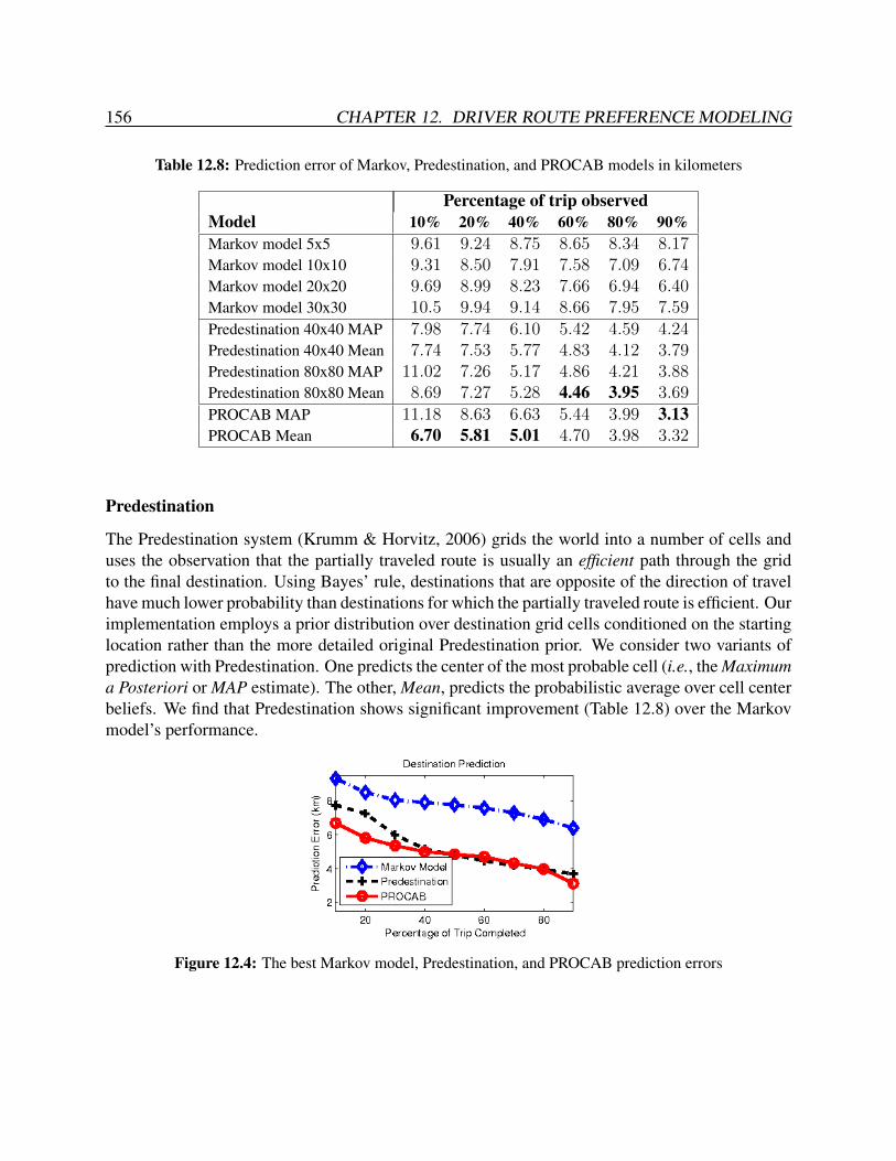
156 CHAPTER 12. DRIVER ROUTE PREFERENCE MODELING
Table 12.8: Prediction error of Markov, Predestination, and PROCAB models in kilometers
Percentage of trip observedModel 10% 20% 40% 60% 80% 90%Markov model 5x5 9.61 9.24 8.75 8.65 8.34 8.17Markov model 10x10 9.31 8.50 7.91 7.58 7.09 6.74Markov model 20x20 9.69 8.99 8.23 7.66 6.94 6.40Markov model 30x30 10.5 9.94 9.14 8.66 7.95 7.59Predestination 40x40 MAP 7.98 7.74 6.10 5.42 4.59 4.24Predestination 40x40 Mean 7.74 7.53 5.77 4.83 4.12 3.79Predestination 80x80 MAP 11.02 7.26 5.17 4.86 4.21 3.88Predestination 80x80 Mean 8.69 7.27 5.28 4.46 3.95 3.69PROCAB MAP 11.18 8.63 6.63 5.44 3.99 3.13PROCAB Mean 6.70 5.81 5.01 4.70 3.98 3.32
Predestination
The Predestination system (Krumm & Horvitz, 2006) grids the world into a number of cells anduses the observation that the partially traveled route is usually an efficient path through the gridto the final destination. Using Bayes’ rule, destinations that are opposite of the direction of travelhave much lower probability than destinations for which the partially traveled route is efficient. Ourimplementation employs a prior distribution over destination grid cells conditioned on the startinglocation rather than the more detailed original Predestination prior. We consider two variants ofprediction with Predestination. One predicts the center of the most probable cell (i.e., the Maximuma Posteriori or MAP estimate). The other, Mean, predicts the probabilistic average over cell centerbeliefs. We find that Predestination shows significant improvement (Table 12.8) over the Markovmodel’s performance.
Figure 12.4: The best Markov model, Predestination, and PROCAB prediction errors

12.7. DISCUSSION 157
PROCAB Destination Prediction
In the PROCAB model, destination prediction is also an application of Bayes’ rule. Consider apartial path, ζA→B from point A to point B. The destination probability is then:
P(dest|ζA→B, θ) ∝ P(ζA→B|dest, θ) P(dest)
∝∑
ζB→destereward(ζ|θ)∑
ζA→destereward(ζ|θ) P(dest) (12.2)
We use the same prior that depends on the starting point (A) that we employed in our Predestina-tion implementation. The posterior probabilities are efficiently computed by taking the sums overpaths from points A and B to each possible destination (Equation 12.2) using the forward pass ofAlgorithm 1.
Table 12.8 and Figure 12.4 show the accuracy of PROCAB destination prediction comparedwith other models. Using averaging is much more beneficial for the PROCAB model, likely be-cause it is more sensitive to particular road segments than models based on grid cells. We find thatthe PROCAB model performs comparably to the Predestination model given a large percentage ofobserved trip, and better than the Predestination model when less of the trip is observed. PRO-CAB’s abilities to learn non-travel time desirability metrics, reason about road segments ratherthan grid cells, and incorporate additional contextual information may each contribute to this im-provement.
12.7 DiscussionIn this chapter, we have applied the maximum causal entropy approach to prediction tasks in per-sonal navigation. We have demonstrated state-of-the-art performance on turn prediction, route pre-diction, and destination prediction tasks using large-scale data collected from taxi drivers. One ofthe main advantages of our approach—personalization to individual drivers driving preferences—is not well-explored by this approach, since taxi drivers are typically optimizing for travel-timerather than e.g., avoiding certain types of driving for safety reasons. We expect an even largerperformance improvement over more naıve approaches on prediction tasks for non-professionaldrivers.

Chapter 13
Pedestrian Motion Prediction
“Real men usually voluntarily avoid robots”— Tadokoro et al. (1995)
In this chapter, we apply the maximum causal entropy framework to the problem of predictingthe future movements of a pedestrian within an indoor environment. Accurate predictions in thistask are important for planning intelligent robot movements that appropriately balance the desireto have the robot efficiently reach its destination with the desire not to hinder peoples’ movementsin the environment.
13.1 MotivationsDetermining appropriate robotic actions in environments with moving people is a well-studied (Ta-dokoro et al., 1995; Bennewitz et al., 2002; Foka & Trahanias, 2002), but often difficult task due tothe uncertainty of each person’s future behavior. Robots should certainly never collide with people(Petti & Fraichard, 2005), but avoiding collisions alone is often unsatisfactory because the disrup-tion of almost colliding can be burdensome to people and sub-optimal for robots. Instead, robotsshould predict the future locations of people and plan routes that will avoid such hindrances (i.e.,situations where the person’s natural behavior is disrupted due to a robot’s proximity) while stillefficiently achieving the robot’s objectives. For example, given the origins and target destinationsof the robot and person in Figure 13.1, the robot’s hindrance-minimizing trajectory would take thelonger way around the center obstacle (a table), leaving a clear path for the pedestrian.
One common approach for predicting trajectories is to project the prediction step of a track-ing filter (Madhavan & Schlenoff, 2003; Schlenoff et al., 2004; Mertz, 2004) forward over time.For example, a Kalman filter’s (Kalman & Bucy, 1962) future positions are distributed accordingto a Gaussian distribution with growing uncertainty and, unfortunately, often high probability forphysically impossible locations (e.g., behind walls, within obstacles). Particle filters (Thrun et al.,2005) can incorporate more sophisticated constraints and non-Gaussian distributions, but degrade
158
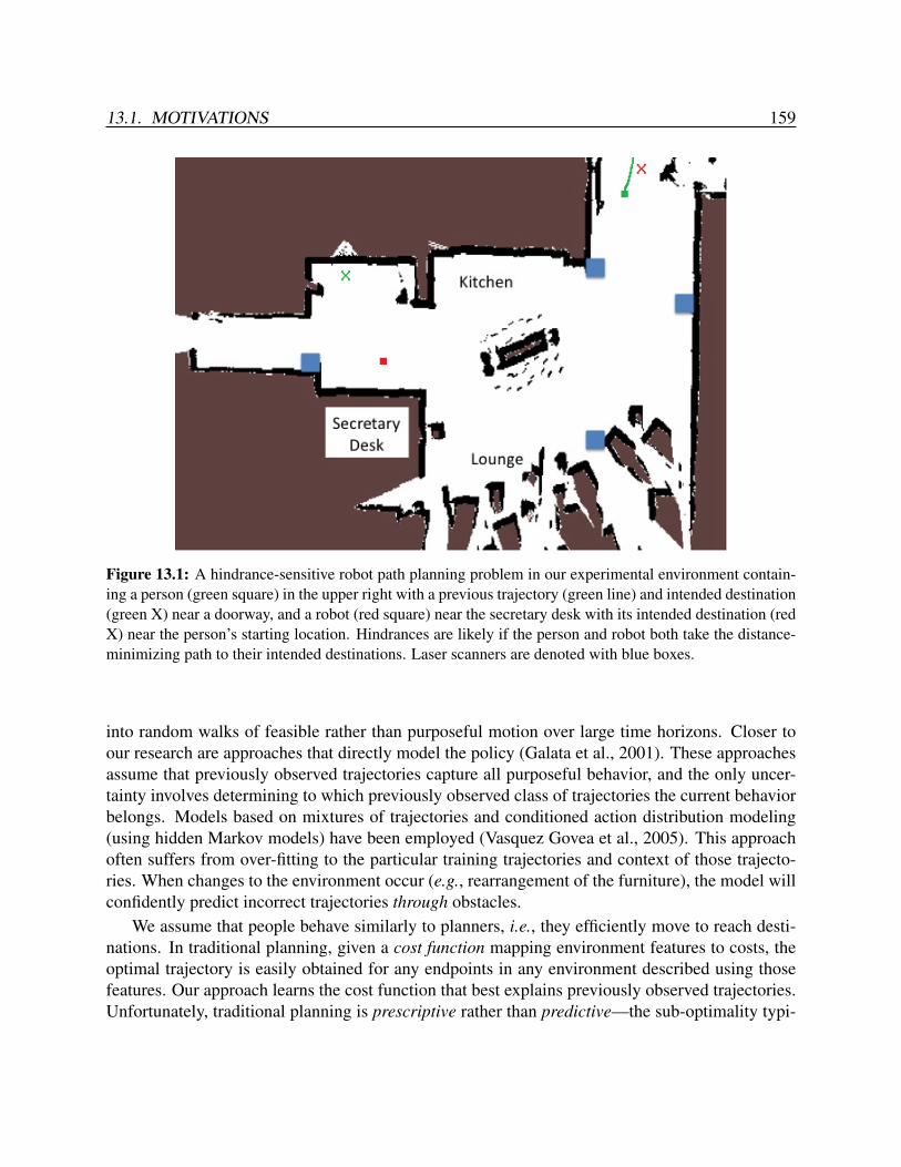
13.1. MOTIVATIONS 159
Figure 13.1: A hindrance-sensitive robot path planning problem in our experimental environment contain-ing a person (green square) in the upper right with a previous trajectory (green line) and intended destination(green X) near a doorway, and a robot (red square) near the secretary desk with its intended destination (redX) near the person’s starting location. Hindrances are likely if the person and robot both take the distance-minimizing path to their intended destinations. Laser scanners are denoted with blue boxes.
into random walks of feasible rather than purposeful motion over large time horizons. Closer toour research are approaches that directly model the policy (Galata et al., 2001). These approachesassume that previously observed trajectories capture all purposeful behavior, and the only uncer-tainty involves determining to which previously observed class of trajectories the current behaviorbelongs. Models based on mixtures of trajectories and conditioned action distribution modeling(using hidden Markov models) have been employed (Vasquez Govea et al., 2005). This approachoften suffers from over-fitting to the particular training trajectories and context of those trajecto-ries. When changes to the environment occur (e.g., rearrangement of the furniture), the model willconfidently predict incorrect trajectories through obstacles.
We assume that people behave similarly to planners, i.e., they efficiently move to reach desti-nations. In traditional planning, given a cost function mapping environment features to costs, theoptimal trajectory is easily obtained for any endpoints in any environment described using thosefeatures. Our approach learns the cost function that best explains previously observed trajectories.Unfortunately, traditional planning is prescriptive rather than predictive—the sub-optimality typi-
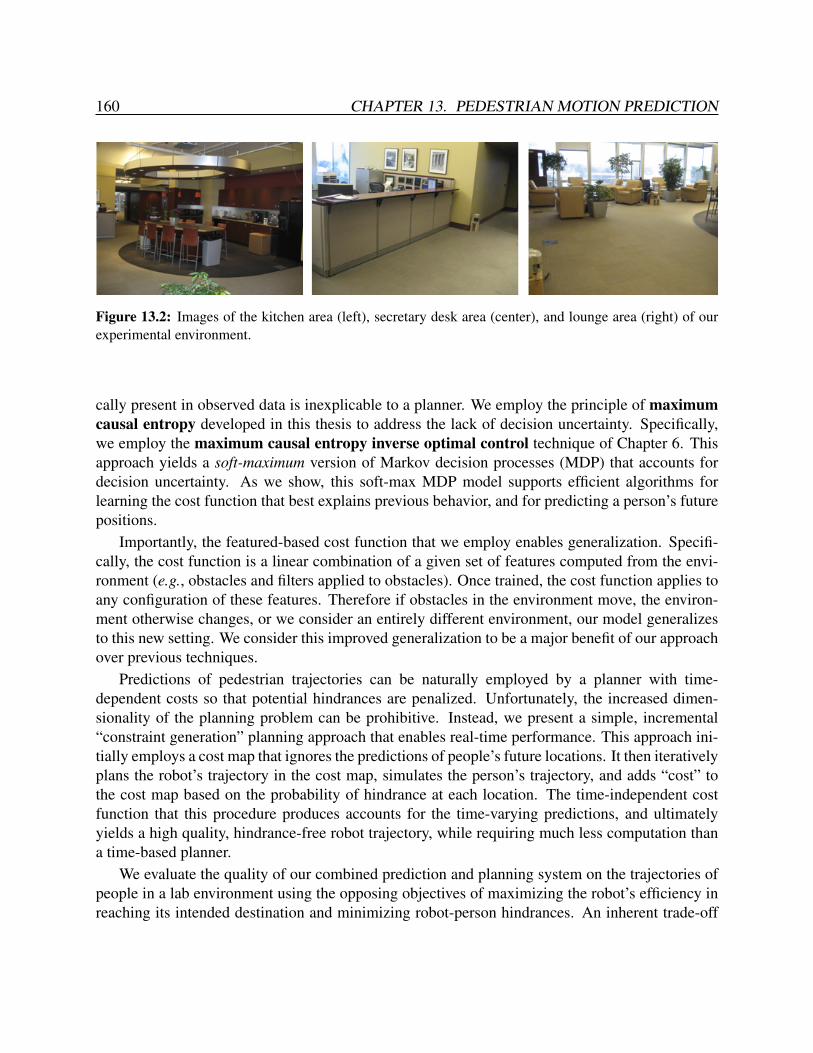
160 CHAPTER 13. PEDESTRIAN MOTION PREDICTION
Figure 13.2: Images of the kitchen area (left), secretary desk area (center), and lounge area (right) of ourexperimental environment.
cally present in observed data is inexplicable to a planner. We employ the principle of maximumcausal entropy developed in this thesis to address the lack of decision uncertainty. Specifically,we employ the maximum causal entropy inverse optimal control technique of Chapter 6. Thisapproach yields a soft-maximum version of Markov decision processes (MDP) that accounts fordecision uncertainty. As we show, this soft-max MDP model supports efficient algorithms forlearning the cost function that best explains previous behavior, and for predicting a person’s futurepositions.
Importantly, the featured-based cost function that we employ enables generalization. Specifi-cally, the cost function is a linear combination of a given set of features computed from the envi-ronment (e.g., obstacles and filters applied to obstacles). Once trained, the cost function applies toany configuration of these features. Therefore if obstacles in the environment move, the environ-ment otherwise changes, or we consider an entirely different environment, our model generalizesto this new setting. We consider this improved generalization to be a major benefit of our approachover previous techniques.
Predictions of pedestrian trajectories can be naturally employed by a planner with time-dependent costs so that potential hindrances are penalized. Unfortunately, the increased dimen-sionality of the planning problem can be prohibitive. Instead, we present a simple, incremental“constraint generation” planning approach that enables real-time performance. This approach ini-tially employs a cost map that ignores the predictions of people’s future locations. It then iterativelyplans the robot’s trajectory in the cost map, simulates the person’s trajectory, and adds “cost” tothe cost map based on the probability of hindrance at each location. The time-independent costfunction that this procedure produces accounts for the time-varying predictions, and ultimatelyyields a high quality, hindrance-free robot trajectory, while requiring much less computation thana time-based planner.
We evaluate the quality of our combined prediction and planning system on the trajectories ofpeople in a lab environment using the opposing objectives of maximizing the robot’s efficiency inreaching its intended destination and minimizing robot-person hindrances. An inherent trade-off

13.2. PLANNING WITH PEDESTRIAN PREDICTIONS 161
Algorithm 13.1 Incorporating predictive pedestrian models via predictive planning
1: PredictivePlanning( σ > 0, α > 0, {Ds,t}, Dthresh )2: Initialize cost map to prior navigational costs c0(s).3: for t = 0, . . . , T do4: Plan under the current cost map.5: Simulate the plan forward to find points of probable interference with the pedestrian
{(si)}Kti=1 where Ds,t > Dthresh.6: If K = 0 then break.7: Add cost to those points8: ct+1(s) = ct(s) + α
∑Kti=1 e
− 12σ2‖s−si‖2 .
9: end for10: Return the plan through the final cost map.
between these two criteria exists in planning appropriate behavior. We show that for nearly anychosen trade-off, our prediction model is better for making decisions than an alternate approach.
13.2 Planning with Pedestrian Predictions
13.2.1 Temporal Predictions
To plan appropriately requires predictions of where people will be at different points in time.More formally, we need predictions of expected future occupancy of each location during the timewindows surrounding fixed intervals: τ, 2τ, ..., T τ . We denote these quantities as Ds,t. In theory,time can be added to the state space of a Markov decision process and explicitly modeled. Inpractice, however, this expansion of the state space significantly increases the time complexity ofinference, making real-time applications based on the time-based model impractical. We insteadconsider an alternative approach that is much more tractable.
We assume that a person’s movement will “consume” some cost over a time window t accord-ing to the normal distribution N(tC0, σ
20 + tσ2
t ), where C0, σ20 , and σ2
t are learned parameters.Certainly
∑tDs,t = Ds, so we simply divide the expected visitation counts among the time inter-
vals according to this probability distribution. We use the cost of the optimal path to each state,Q∗(s), to estimate the cost incurred in reaching it. The resulting time-dependent occupancy countsare then:
Ds,it ∝ Dse−(C0t−Q
∗(s))2
2(σ20+tσ21) . (13.1)
These values are computed using a single execution of Dijkstra’s algorithm (Dijkstra, 1959) inO(|S| log |S|) time to compute Q∗(.) and then O(|S|T ) time for additional calculation.

162 CHAPTER 13. PEDESTRIAN MOTION PREDICTION
Ideally, to account for predictive models of pedestrian behavior, we should increase the di-mensionality of the planning problem by augmenting the state of the planner to account for time-varying costs. Unfortunately, the computational complexity of combinatorial planning is exponen-tial in the dimension of the planning space, and the added computational burden of this solutionwill be prohibitive for many real-time applications.
We therefore propose a novel technique for integrating our time-varying predictions into therobot’s planner. Algorithm 13.1 details this procedure; it essentially iteratively shapes a time-independent navigational cost function to remove known points of hindrance. At each iteration,we run the time-independent planner under the current cost map and simulate forward the resultingplan in order to predict points at which the robot will likely interfere with the pedestrian. By thenadding cost to those regions of the map we can ensure that subsequent plans will be discouragedfrom interfering at those locations. We can further improve the computational gain of this tech-nique by using efficient replanners such as D* and its variants (Ferguson & Stentz, 2005) in theinner loop. While this technique, as it reasons only about stationary costs, cannot guarantee theoptimal plan given the time-varying costs, we demonstrate that it produces good robot behavior inpractice that efficiently accounts for the predicted motion of the pedestrian.
By re-running this iterative replanner every 0.25 seconds using updated predictions of pedes-trian motion, we can achieve intelligent adaptive robot behavior that anticipates where a pedestrianis heading and maneuvers well in advance to implement efficient avoidance. In practice, we use thefinal cost-to-go values of the iteratively constructed cost map to implement a policy that choosesa good action from a predefined collection of actions. When a plan with sufficiently low prob-ability of pedestrian hindrance cannot be found, the robot’s speed is varied. Additionally, whenthe robot is too close to a pedestrian, all actions that take the robot within a small radius of thehuman are removed to avoid potential collisions. Section 13.3.6 presents quantitative experimentsdemonstrating the properties of this policy.
13.3 Experimental EvaluationWe now present experiments demonstrating the capabilities of our prediction model and its useful-ness for planning hindrance-sensitive robot trajectories.
13.3.1 Data CollectionWe collected over one month’s worth of data in a lab environment. The environment has threemajor areas (Figure 13.1): a kitchen area with a sink, refrigerator, microwave, and coffee maker; asecretary desk; and a lounge area. We installed four laser range finders in fixed locations aroundthe lab, as shown in Figure 13.1, and ran a pedestrian tracking algorithm (MacLachlan, 2005).Trajectories were segmented based on significant stopping time in any location.
From the collected data, we use a subset of 166 trajectories through our experimental envi-ronment to evaluate our approach. This dataset is shown in Figure 13.3 after post-processing and

13.3. EXPERIMENTAL EVALUATION 163
Figure 13.3: Collected trajectory dataset.
being fit to a 490 by 321 cell grid (each cell represented as a single pixel). We employ 50% ofthis data as a training set for estimating the parameters of our model and use the remainder forevaluative purposes.
13.3.2 Learning Feature-Based Cost FunctionsWe learn a 6-parameter cost function over simple features of the environment, which we argueis easily transferable to other environments. The first feature is a constant feature for every gridcell in the environment. The remaining functions are an indicator function for whether an obstacleexists in a particular grid cell, and four “blurs” of obstacle occupancies, which are shown in Figure13.4.
Figure 13.4: Four obstacle-blur features for our cost function. Feature values range from low weight (darkblue) to high weight (dark red).
We then learn the weights for these features that best explain the demonstrated data. The result-ing cost function for the environment is shown in Figure 13.5. Obstacles in the cost function have

164 CHAPTER 13. PEDESTRIAN MOTION PREDICTION
very high cost, and free space has a low cost that increases near obstacles. Essentially, the predic-tive model learns that travel through obstacles is extremely expensive and that travel near obstaclesis costly, but not as expensive, relative to travel through open space. Despite the simplicity of thelearned model, it generalizes well and provides useful predictions in practice.
Figure 13.5: Left: The learned cost function in the environment. Right: The prior distribution over destina-tions learned from the training set.
The prior distribution over destinations is obtained from the set of endpoints in the training set,and the temporal Gaussian parameters are also learned using the training set.
13.3.3 Stochastic Modeling ExperimentWe first consider two examples from our dataset (Figure 13.6) that demonstrate the need foruncertainty-based modeling.
Figure 13.6: Two trajectory examples (blue) and log occupancy predictions (red).
Both trajectories travel around the table in the center of the environment. However, in the firstexample (left), the person takes the lower pathway around the table, and in the second example

13.3. EXPERIMENTAL EVALUATION 165
(right), the person takes the upper pathway despite that the lower pathway around the table has alower cost in the learned cost function. In both cases, the path taken is not the shortest path throughthe open space that one would obtain using an optimal planner. Our uncertainty-based planningmodel handles these two examples appropriately, while a planner would choose one pathway or theother around the table and, even after smoothing the resulting path into a probability distribution,tend to get a large fraction of its predictions wrong when the person takes the “other” approximatelyequally desirable pathway.
13.3.4 Dynamic Feature Adaptation Experiment
In many environments, the relevant features that influence movement change frequently: furnitureis moved in indoor environments; the locations of parked vehicles are dynamic in urban environ-ments; and weather conditions influence natural environments with muddy, icy, or dry conditions.We demonstrate qualitatively that our model of motion is robust to these feature changes.
The left frames of Figure 13.7 show the environment and the path prediction of a person movingaround the table at two different points in time. At the second point of time (bottom left), theprobability of the trajectory leading to the kitchen area or the left hallway is extremely small. Inthe right frames of Figure 13.7, an obstacle has been introduced that blocks the direct pathwaythrough the kitchen area. In this case, the trajectory around the table (bottom right) still has a veryhigh probability of leading to either the kitchen area or the left hallway. As this example shows,our approach is robust to changes in the environment such as this one.
13.3.5 Comparative Evaluation
We now compare our model’s ability to predict the future path of a person with a previous approachfor modeling goal-directed trajectories – the variable-length Markov model (VLMM) (Galata et al.,2001). The VLMM (introduced in Section 3.1.1) estimates the probability of a person’s next celltransition conditioned on the person’s history of cells visited in the past. It is variable lengthbecause it employs a long history when relevant training data is abundant, and a short historyotherwise.
The results of our experimental evaluation are shown in Figure 13.8. We first note that for thetraining set (denoted train), that the trajectory log probability of the VLMM is significantly betterthan the plan-based model. However, for the test set, which is the metric we actually care about,the performance of the VLMM degrades significantly, while the degradation in the plan-basedmodel is much less extreme. We conclude from this experiment that the VLMM (and similardirected graphical model approaches) are generally much more difficult to train to generalize wellbecause their number of parameters is significantly larger than the number of parameters of thecost function employed in our approach.

166 CHAPTER 13. PEDESTRIAN MOTION PREDICTION
Figure 13.7: Our experimental environment with (right column) and without (left column) an added ob-stacle (gray, indicated by an arrow) between the kitchen and center table (with white arrow for emphasis).Predictions of future visitation expectations given a person’s trajectory (white line) in both settings for twodifferent trajectories. Frequencies range from red (high log expectation) to dark blue (low log expectation).
13.3.6 Integrated Planning Evaluation
We now simulate robot-human hindrance problems to demonstrate the benefit of our trajectoryforecasting approach. We generate 200 hindrance-sensitive planning problems (corresponding to22 different person trajectories in Figure 13.3) by selecting problems where naıve planning (disre-garding the pedestrian) causes hindrances. We ignore the causal influence of the robot’s action onthe person’s trajectory, and measure the trade-off between robot efficiency and interference withthe person’s trajectory. Specifically, the average hindrance count measures the average numberof times the policy removed actions due to proximity to a human, and the average execution timemeasures the number of time steps needed to reach the goal. The trade-off is controlled by vary-ing the degree of the visitation frequency threshold used in Algorithm 13.1. The robot trajectoryplanner is provided with person location forecasts at 4Hz.
The trade-off curves of planning using our plan-based forecasts and using a straight-forwardparticle-based forecasting model on this set of problems are shown in Figure 13.9. For both pre-

13.4. DISCUSSION 167
Figure 13.8: Log probability of datasets under the VLMM and our approach.
dictive models, while the execution time varies over a small range, the average hindrance countdecreases by a factor of two. Additionally, as the figure shows, the plan-based forecasting is supe-rior to the particle-based approach for almost any level of the trade-off.
13.4 DiscussionIn this chapter, we have demonstrated the effective use of the maximum causal entropy approachfor improving the navigation decisions of a robot. We employ a sophisticated predictions of thefuture positions of pedestrians within the robot’s environment. The path planning employed by ourapproach does not employ inverse optimal control to learn the cost for robot navigation; it uses afixed cost function to deter movements leading to hindrances.
Recently a complementary maximum entropy inverse optimal control has been employed toalso improve robot navigation among people. This technical approach was extended to addresssettings with partial information. Whereas we use the inverse optimal control approach to modelpedestrian behavior and employ the predictions in a cost function, Henry et al. (2010) pose theproblem of path planning for a robot as a supervised problem and extend our maximum entropyapproach to deal with partial observability of a probabilistic model of crowds of pedestrian move-ments. Combining these two approaches, or learning to adjust the robot’s planner from interactionwith pedestrians, is an important future direction for this line of research.
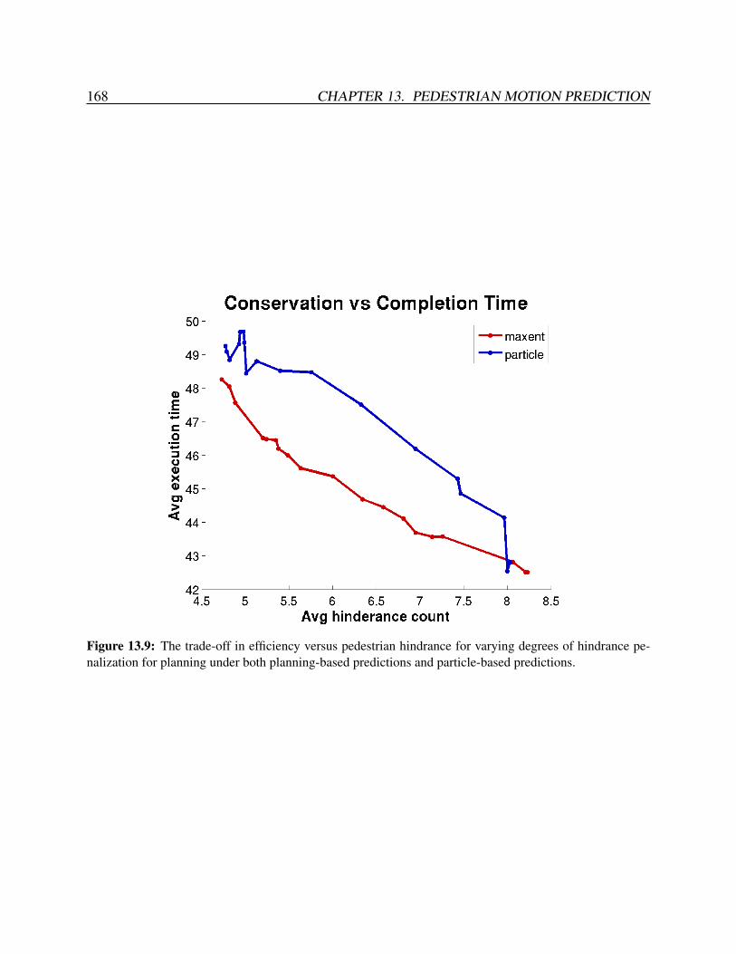
168 CHAPTER 13. PEDESTRIAN MOTION PREDICTION
Figure 13.9: The trade-off in efficiency versus pedestrian hindrance for varying degrees of hindrance pe-nalization for planning under both planning-based predictions and particle-based predictions.

Chapter 14
Other Applications
“Life is a sum of all your choices”— Albert Camus (Philosopher, 1913–1960)
We now present three additional applications with varying complexity of interaction: the firstis interactions of multiple players within a correlated equilibrium, the second is interaction with apartially observable system, and the third is inverse linear quadratic regulation.
14.1 Maximum Causal Entropy Correlated Equilibria for MarkovGames
Using the theory developed in Chapter 8 for rational behavior in multi-player games, we presentexperiments for the robust prediction of rational behavior in stochastic games.
14.1.1 Experimental SetupFollowing Zinkevich et al. (2006), we generate random stochastic Markov games according to thefollowing procedure. For each of |S| states in the Markov game, each of N players has |A| actionsto choose from (for a total of |A|N joint actions). The state transition dynamics, {P(st+1|st, a1:N
t )},depend on the combination of players’ actions (and state) and are drawn uniformly from the sim-plex of probabilities. The utility obtained by each player in each state, Utilityi(s), is drawn uni-formly from {0, 0.1, 0.2, ..., 0.9}. For our experiments, we allow either the number of states to varywith 2 actions and 3 players; or the number of players to vary for random Markov games with 2states and 2 actions. In both cases, we employ a discount factor of γ = 0.75. We consider a fixedtime horizon of T = 10 time steps for our experiments.
We generate time-varying strategy profiles for MCECE using Algorithm 9.13 and for the CE-Qvariants using projected sub-gradient optimization. The CE-Q strategies we evaluate are a subset
169

170 CHAPTER 14. OTHER APPLICATIONS
of those described in Section 8.1.2. iCEQ maximizes the positive margin of player 1’s utility overplayer 2’s utility. We repeat this process for 100 random games for each choice of game parametersand investigate the properties of the resulting CE strategy profiles.
14.1.2 EvaluationWhile the joint entropy of trajectories through a game tends to greatly increase with the numberof states due to increased transition dynamic stochasticity, the uncertainty of the per-state actionuncertainty does not, as shown in Figure 14.1.
Figure 14.1: The (log2) causal entropy measure of the inherent difficulty of predicting the 10 time stepaction sequences that are generated by different correlated equilibria solution concepts’ strategy profiles forvarying numbers of states (left) with 2 actions and 3 players, and for varying numbers of players (right) with2 actions and 2 states. It can be interpreted as the number of binary bits needed on average to represent theactions of a sampled trajectory under the strategy profile’s distribution.
In fact, actions become slightly more predictable with more states, presumably due to theavailability of more diverse action outcomes that better satisfy multiple players’ objectives. Bycontrast, the uncertainty of action sequences increases logarithmically with the size of the actionset, as one might expect. We note that in all cases, the MCECE strategy profile is the most uncertain(by design), and many of the previously investigated CE-Q solutions are the most deterministic.
The log probability of samples from one strategy profile under another strategy profile (i.e., thelog-loss or cross entropy),
−∑a1:N
πA(a1:N) log πB(a1:N), (14.1)
is a common, but harsh metric for evaluating the predictive capabilities of strategy profile B; itpenalizes infinitely for actions with non-zero probability in A, but zero probability in B. Instead,

14.2. INVERSE DIAGNOSTICS 171
Table 14.1: The average cross-strategy-profile predictability for the single time step action distribution fromthe initial game state averaged over 100 random 3-player, 2-state, 2-action Markov games. Denoted are thepercentage of strategies that are impossible to represent in the strategy profile (i.e., having zero probabilitywithin the model). and the average number of bits needed to encode the combined action of those that areimpossible to represent. We only count strategies with 0.1% probability or more under the predicted strategyprofile for assessing representation possibility and never penalize more than 16.6 bits (− log2 0.00001) forany extremely small probability in the predicting strategy profile to avoid any approximation effects—bothto the benefit of CE-Q strategy profiles.
MCECE uCE-Q d1CE-Q d2CE-Q x1CE-Q x2CE-Q iCE-Q Average
MCECE ——–1.951 1.951 1.967 2.010 1.992 1.974 1.9740.0% 0.0% 0.0% 0.0% 0.0% 0.0% 0.0%
uCE-Q3.377
——–2.039 1.888 2.647 3.072 2.444 2.578
22.3% 4.5% 5.7% 21.2% 20.8% 13.8% 14.7%
d1CE-Q3.442 1.866
——–2.511 3.328 2.321 1.798 2.544
18.9% 3.5% 5.6% 18.8% 17.6% 9.8% 12.4%
d2CE-Q3.462 1.872 2.536
——–2.576 3.489 3.060 2.833
17.0% 1.7% 3.3% 15.6% 17.2% 12.1% 11.2%
x1CE-Q2.897 2.472 2.798 2.450
——–2.375 2.764 2.626
0.2% 0.0% 0.0% 0.0% 0.0% 0.0% 0.0%
x2CE-Q2.877 2.605 2.251 2.905 2.373
——–2.116 2.521
0.5% 0.0% 0.0% 0.0% 0.2% 0.0% 0.1%
iCE-Q3.378 2.279 1.902 2.989 3.116 2.276
——–2.657
5.3% 1.9% 0.0% 2.5% 5.1% 4.2% 3.2%
we extend the representational interpretation of the log probability and assess what fraction ofsamples in A are possible to represent in B and of the ones possible to represent, the averagenumber of bits required to do so, −
∑a1:N :πB(a1:N )>0 πA(a1:N) log πB(a1:N)).
The results of this comparison across strategy profiles is shown in Table 14.1 (for 3 players) andTable 14.2 (for 4 players). We note that in some cases one C-EQ strategy profile may better predictanother than the MCECE strategy profile when their objectives are closely aligned. For example,the x2CE-Q tends to predict iCE-Q fairly accurately since both are punishing player 2 to somedegree. However, overall the MCECE solution profile provides a much more robust prediction ofother strategy profiles on average and full support of all possible action combinations.
14.2 Inverse DiagnosticsMany important problems can be framed as interaction with a partially observable stochastic sys-tem. In medical diagnosis, for example, tests are conducted, the results of which may lead toadditional tests to narrow down probable conditions or diseases and to prescribe treatments, which

172 CHAPTER 14. OTHER APPLICATIONS
Table 14.2: The average cross-strategy-profile single action predictability for 4 players and otherwise theidentical experimental setting as Table 14.1.
MCECE uCE-Q d1CE-Q d2CE-Q x1CE-Q x2CE-Q iCE-Q Average
MCECE ——–3.451 3.468 3.476 3.518 3.509 3.475 3.4830.0% 0.0% 0.0% 0.0% 0.0% 0.0% 0.0%
uCE-Q7.308
——–3.955 3.652 6.495 6.814 5.591 5.636
25.8% 9.4% 8.5% 21.8% 22.0% 17.9% 17.6%
d1CE-Q6.914 3.831
——–4.746 7.566 5.536 3.895 5.415
22.5% 5.8% 10.2% 21.2% 17.6% 11.2% 14.8%
d2CE-Q7.109 3.408 4.767
——–5.643 7.651 6.976 5.926
23.1% 6.4% 10.7% 18.3% 21.5% 19.7% 16.6%
x1CE-Q4.603 4.300 5.000 3.849
——–3.918 4.372 4.340
0.0% 0.0% 0.0% 0.0% 0.0% 0.0% 0.0%
x2CE-Q4.633 4.401 3.917 4.986 3.944
——–3.171 4.175
0.1% 0.0% 0.0% 0.0% 0.0% 0.0% 0.0%
iCE-Q6.380 5.070 3.884 6.501 5.991 4.311
——–5.356
11.5% 5.0% 2.8% 8.0% 8.7% 5.5% 6.9%
are adjusted based on patient response. Motivated by the objective of learning good diagnosispolicies from experts, we investigate the Inverse Diagnostics problem of modeling interaction withpartially observed systems.
14.2.1 MaxCausalEnt ID Formulation
In this setting, the partially observed set of variables (related by a Bayesian Network in this appli-cation) serves as side information. Inference over the latent variables from this set is required toinfer decision probabilities. Additionally, decisions can influence the variables, causally changingtheir values, and the implications of these interventions must also be assessed. Vectors of featuresare associated with observing or manipulating each variable, and we employ our MaxCausalEntID model with these features as value nodes as shown in Figure 14.21.
14.2.2 Fault Diagnosis Experiments
We apply our inverse diagnostics approach to the vehicle fault detection Bayesian Network (Heck-erman et al., 1994) shown in Figure 14.3. Apart from the relationship between Battery Age andBattery (exponentially increasing probability of failure with battery age), the remaining condi-
1An objective function over the Bayesian Network variables can also be incorporated into a value node at eachtime-step and/or at the end of the sequence, as shown.

14.2. INVERSE DIAGNOSTICS 173
Figure 14.2: The MaxCausalEnt ID representation of the diagnostic problem.
Figure 14.3: The vehicle fault detection Bayesian Network.
tional probability distributions are deterministic-or’s (i.e., failure in any parent causes a failure inthe child). The remaining (conditional) probabilities is shown in Table 14.3.
Table 14.3: Probability distributions governing random variables in the vehicle fault diagnosis Bayesiannetwork of the inverse diagnostics experiment.
P (battery age = x) =1
5for x = 0, 1, 2, 3, 4
P (starter failure) = 0.005
P (fuel pump failure) = 0.002
P (fuel failure) = 0.006
P (spark plug failure) = 0.003
P (battery failure|battery age) = 1− e−.01∗battery age
Each variable in the network can be tested, revealing whether it is operational (or the battery’sage), and the Battery, Fuel, Fuel Line, Fuel Pump, Spark Plugs, and Starter can each be replaced

174 CHAPTER 14. OTHER APPLICATIONS
(making it and potentially its descendants operational). Replacements and tests are both character-ized action features: a cost to the vehicle owner, a profit for the mechanic, and a time requirement.Ideally a sequence of tests and replacements would minimize the expected cost to the vehicleowner, but an over-booked mechanic might instead choose to minimize the total repair time so thatother vehicles can be serviced, and a less ethical mechanic might seek to optimize personal profit.
Table 14.4: Replacement and observation features for variables of the vehicle fault diagnosis Bayesiannetwork. The first feature corresponds to an approximate cost to the vehicle owner. The second featurecorresponds to an approximate profit to the mechanic. The final feature corresponds to a time requirement.
Variable Replace Features Observation FeaturesBattery Age [5.0, 5.0, 0.0]
Starter [120.0, 100.0, 40.0] [60.0, 30.0, 20.0]Fuel Pump [150.0, 120.0, 30.0] [70.0, 40.0, 20.0]Fuel Line [50.0, 30.0, 15.0] [40.0, 20.0, 15.0]
Fuel [30.0, 25.0, 10.0] [15.0, 10.0, 5.0]Batter [140.0, 120.0, 20.0] [50.0, 30.0, 20.0]
Engine Turns Over [5.0, 5.0, 3.0]Fuel Subsystem [10.0, 10.0, 5.0]
Fuel Gauge [3.0, 3.0, 2.0]Lights [2.0, 2.0, 2.0]
Spark Plugs [90.0, 60.0, 40.0] [50.0, 30.0, 20.0]Engine Starts [5.0, 5.0, 3.0]
To generate a dataset of observations and replacements, a stochastic policy is obtained byadding Gaussian noise, εs,a, to each action’s future expected value, Q∗(s, a), under the optimalpolicy for a fixed set of weights and selecting the highest noisy-valued action, Q∗(s, a) + εs,a,to execute at each time-step. Different vehicle failure samples are generated from the BayesianNetwork conditioned on the vehicle’s engine failing to start, and the stochastic policy is sampleduntil the vehicle is operational.
We evaluate the prediction error rate and log-loss of our model in Figure 14.4. We compareagainst a Markov Model that ignores the underlying mechanisms for decision making and sim-ply predicts behavior in proportion to the frequency it has previously been observed (with smallpseudo-count priors). Our approach consistently outperforms the Markov Model even with an or-der of magnitude less training data. The classification error rate quickly reaches the limit impliedby the inherent stochasticity of the data generation process.

14.3. HELICOPTER CONTROL 175
Figure 14.4: Error rate and log-loss of the MaxCausalEnt ID model and Markov Model for diagnosis actionprediction as training set size (log-scale) increases.
14.3 Helicopter ControlWe demonstrate the MaxCausalEnt approach to inverse stochastic optimal control on the prob-lem of building a controller for a learned helicopter model (Abbeel et al., 2007) with linearizedstochastic dynamics. Most existing approaches to inverse optimal control with stochastic dynam-ics (Ratliff et al., 2006; Abbeel & Ng, 2004) have both practical and theoretical difficulties in thepresence of imperfect demonstrated behavior, leading to unstable controllers due to large changesin cost weights (Abbeel et al., 2007) or poor predictive accuracy (Ratliff et al., 2006).
14.3.1 Experimental Setup
To test the robustness of our approach, we generated five 100 timestep sub-optimal training tra-jectories by noisily sampling actions from an optimal LQR controlled designed for hovering usingthe linearized stochastic simulator of Abbeel et al. (2007). It simulates a XCell Tempest helicopterusing four continuous control variables: elevator, aileron, rudder, main rotor; and a 21 dimensionalstate space: position, orientation, velocity, angular rate, previous controls, and change in previouscontrols.
14.3.2 Evaluation
We contrast performance between maximum margin planning (Ratliff et al., 2006) (labeled IN-VOPT in Figure 14.5) and MaxCausalEnt trained using demonstrated trajectories. Performancewas evaluated by generating trajectories from the optimal controller of each model and measuringtheir cost under the true cost function used to generate the original sub-optimal demonstration tra-jectories. The InvOpt model performs poorly because there is no optimal trajectory for any costfunction that matches demonstrated features.
On the other hand, the function learned by MaxCausalEnt IOC not only induces the same

176 CHAPTER 14. OTHER APPLICATIONS
Figure 14.5: Left: An example sub-optimal helicopter trajectory attempting to hover around the origin point.Right: The average cost under the original cost function of: (1) demonstrated trajectories; (2) the optimalcontroller using the inverse optimal control model; and (3) the optimal controller using the maximum causalentropy model.
feature counts– and hence equal cost on the unknown cost function– under the learned probabilisticpolicy, but because of the quadratic cost function its learned controller’s optimal policy is alwaysat least as good as the demonstrated behavior on the original, unknown cost function. Figure 14.5demonstrates this; the resulting learned optimal policy outperforms the demonstrated behavior onthe original, unknown cost function. In this sense, MaxCausalEnt provides a rigorous approach tolearning a cost function for such stochastic optimal control problems: it is both predictive and canguarantee good performance of the learned controller.
14.4 DiscussionIn this chapter, we demonstrated three applications of the maximum causal entropy approach thatextend beyond discrete-valued inverse optimal control. Specifically, we investigated the setting ofmultiple rational agents, the setting with additional latent information, and the setting of contin-uous control. These applications help to illustrate the versatility of the maximum causal entropyprinciple.

Part V
Conclusions
177

Chapter 15
Open Problems
“Science never solves a problem without creating ten more.”— George Bernard Shaw (Playwright, 1856–1950).
Throughout this thesis, we have made numerous assumptions about the structural relation-ships among variables and the conditional probability distributions from which side informationis drawn. Specifically, we have assumed that the structure and the probability distributions areknown—both to the agent acting to generate behavior sequences, and to the observer trying tomodel and predict the agent’s future behavior—, that certain restrictions exist on the influence ofdecisions and side information on one another, and that deviation regret constrains the distributionof actions. Many possible extensions to the presented work are based on relaxing these assump-tions in various ways.
15.1 Structure Learning and PerceptionThroughout this thesis, we have assumed that the dynamics governing side information and whichside information influences which decisions are both known. However, in many problem settings,only observed data from a sequential interaction with a stochastic process is available, and learningboth the structural dependencies between variables and probability distributions relating observeddata is a necessary task. Importantly, in the maximum causal entropy model a sequence of vari-ables causally conditioned on another sequence of variables is distributed very differently than asequence statically conditioned on another sequence.
Learning both the structure and distributions relating side information and decision variables isan important direction for future research. In the context of decision making, this is a problem ofmodeling the perception process of the decision maker. A number of important questions follow:
• What classes of structures are indistinguishable from one another given only observationaldata?
178

15.2. PREDICTIVE STRATEGY PROFILES 179
• How efficiently in terms of sample sizes can distinguishable classes of structures be reliablylearned from observational data drawn from a distribution and structure that is in the class ofthe maximum causal entropy framework?
• How computationally efficiently can maximum causal entropy structure learning be per-formed?
• What approximation techniques can be employed to make maximum causal entropy structurelearning more efficient?
• How can theories of perception be incorporated into the structure learning process?
Assuming that the agent knows the structure and distribution of side information variables (butthe learner does not) provides a useful starting point. Relaxing that assumption of agent knowledgeof side information probabilities (and even structure) leads to interesting areas of new researchwhere the maximum causal entropy approach is likely to serve a foundational role.
15.2 Predictive Strategy Profiles
For multi-player settings, existing equilibria solution concepts are largely defined for prescriptivesettings where the actions of an autonomous player (or players) needs to be obtained and em-ployed within a game setting. For predictive settings, most equilibria solution concepts are under-specified—typically they allow multiple solutions and no probabilistic bias over the set of validequilibria to employ as a probability distribution—making them inapplicable without additionalassumptions. Additionally, in numerous experiments (McKelvey & Palfrey, 1992), the actions ofhuman game players often do not follow any rational equilibria solution that game theory pre-scribes.
Predictive models of players’ strategies relax the perfect rationality assumptions of game theoryto allow for bounded rationality, error-prone action selection, and ulterior motives beyond the gamepayoff.
Definition 15.1. In a quantal response equilibrium (McKelvey & Palfrey, 1995, 1998), playersactions are noisily distributed based on the expected utility of the action, typically according to alogit response function. For normal form games, player i’s action choice is distributed accordingto:
P(ai) =eλEP(a)[Utilityi(a)|ai]∑a′ieλEP(a)[Utilityi(a)|a′i]
. (15.1)
180 CHAPTER 15. OPEN PROBLEMS
In the extension to Markov games, the future expected utility is computed based on the assumptionthat the quantal response equilibrium is also played in the future:
P(ati) =eλEP(at)[EUtilityti(at)|ati]∑ati′ eλEP(at)[EUtilityi(at)|ati
′]. (15.2)
A desirable quality of the quantal response equilibrium (Definition 15.1) is that the parameter λcontrols the rationality of the distribution. Namely, as λ goes to infinity, the distribution convergesto a Nash equilibrium.
An alternative model of strategy profiles more explicitly models the bounded rationality ofhuman players.
Definition 15.2. In a level-k model of behavior (Costa-Gomes et al., 2001), a level-k agent playsthe optimal response strategy profile against a level-(k−1) player. A level-0 player chooses actionsuniformly at random.
Recent quantitative evaluations (Wright & Leyton-Brown, 2010) have shown that the com-bination of these two approaches (Stahl & Wilson, 1995) with the model learned and evaluatedthrough a cross-validation procedure provide significantly more accurate predictions than eithermodel alone.
Establishing some form of maximum entropy duality of these existing approaches and general-izing to the setting where features rather than payoffs are known are both important open problems.The formulation, however, must be nuanced; simply enforcing the feature-matching constraints ofinverse optimal control can often lead to predicted behaviors that are highly random and onlyweakly adversarial when given behavior that is highly purposeful and very competitive.
15.3 Closing the Prediction-Intervention-Feedback LoopCreating a closed-loop assistive system that predicts the intentions of human behaviors, executesinterventions on behalf of its users, and assesses feedback from the user to self-improve the entiresystem is the ultimate application goal for the research of this thesis. The predictive techniques,algorithms, and applications described in earlier chapters are one important component of realizingsuch a system. While we believe that accurate behavior predictions are crucial for selecting appro-priate interventions, learning the context-dependent appropriateness of the possible interventionsin terms of those behavior predictions is another important learning problem.
The assistive navigation system application provides a natural testbed for creating closed-loopinterventional feedback system. Many additional interesting settings exist for a such a closed-loopsystem. If an end-task utility is defined according to a known measure, reinforcement learningtechniques can be employed to find intervention strategy that best improve end-task utility. Im-portantly, the adaptation of the user to the intervention strategy is an important aspect to consider.

15.3. CLOSING THE PREDICTION-INTERVENTION-FEEDBACK LOOP 181
When task-level feedback is not as explicit, user adaptation alone can be leveraged to understandwhich intervention strategies are desirable to the user.

Chapter 16
Conclusions and Discussion
“Essentially, all models are wrong, but some are useful.”— George Box (Statistician, 1919–).
We conclude by summarizing and discussing the theoretical and empirical arguments we havepresented in this thesis in support of its central claim:
The principle of maximum causal entropy creates probabilistic models of decisionmaking that are purposeful, adaptive, and/or rational, providing more accurateprediction of human behavior.
16.1 Matching Purposeful CharacteristicsThe premise of our approach has been that many human behaviors are purposeful and that thereare measurable characteristics that differentiate purposeful behavior from non-purposeful behavior.We see this in the vehicle navigation modeling application in the form of destination and roadcharacteristics that define the desirability (or lack thereof) of different road segments of the roadnetwork. In the pedestrian trajectory prediction work, we saw this in the avoidance of obstaclesand areas near obstacles. Statistical models capable of matching those purposeful characteristicsare desired, but they must be capable of generalizing beyond the behavior previously seen.
16.2 Information-Theoretic FormulationThe principle of maximum causal entropy provides the important predictive guarantees of minimaxlog-loss for prediction in the sequential setting. This establishes it as a principled approach formodeling sequential data in a range of decision, control, and game settings where the future is notcompletely controllable. For this guarantee to be of practical importance, the constraints employed
182

16.3. INFERENCE AS SOFTENED OPTIMAL CONTROL 183
within the maximum causal entropy framework must represent the essence of underlying factorsinfluencing the distribution. In the context of behavior modeling, we have focused on constraintson the terminal or goal characteristics of behavior sequences and basis on functions describingstates and actions that can be interpreted as utility or cost potential components.
16.3 Inference as Softened Optimal ControlTo support the purposeful viewpoint, we have established a close algorithmic connection relatinginference in our proposed maximum causal entropy framework to optimal behavior in decisiontheory, planning, and control. Inference in the maximum causal entropy framework can then beviewed as a softened version of the mechanisms employed for optimal decision making. We con-sider this connection to be significant in demonstrating that the models we have developed areinherently biased towards purposeful behavior. Much of the learning problem is then learning theutility function (i.e., cost or reward) that guides behavior sequences in this relaxed analogy of theoptimal decision making model.
16.4 Applications Lending Empirical SupportWe have evaluated the maximum causal entropy approach on prediction tasks in personal naviga-tion, pedestrian movement, assistive control, and multiplayer stochastic games to demonstrate itsperformance in comparison to existing approaches. We have shown improved performance overexisting state-of-the-art techniques for:
• Predicting route selections compared with directed graphical models in the vehicle naviga-tion domain.
• Predicting pedestrian movements compared with filtering-based approaches in the hindrance-sensitive robot planning work.
• Robustly predicting correlated equilibria strategy profiles in Markov games settings.
Additionally, we have shown simple experiments demonstrating the benefits of the approach onthe inverse diagnostics setting where side information is latent and on the inverse linear quadraticregulation setting with continuous states and actions.

Appendix A
Proofs
A.1 Chapter 4 ProofsTheorem 4.22. Generally, the conditional and causal entropies are related as:
H(Y|X) ≤ H(YT ||XT ) ≤ H(Y) ≤ H(Y,X), (A.1)
since additional conditioning can never increase entropy. In the special case that P(XT ||YT−1) isa deterministic function, then:
H(YT ||XT ) = H(Y) = H(Y,X). (A.2)
Proof. If P(XT ||YT−1) is deterministic, H(XT ||YT−1) = 0. By definition, H(Y,X) =H(YT ||XT ) +H(XT ||YT−1), and since H(XT ||YT ) = 0, then H(Y,X) = H(YT ||XT ).
A.2 Chapter 5 ProofsTheorem 5.8. The general maximum causal entropy optimization (Equation 5.6)—or, more cor-rectly, minimizing its negation,
argmin{P(Yt|X1:t,Y1:t−1)}
−H(YT ||XT ) (A.3)
such that: EP(X,Y)[F(X,Y)] = EP(X,Y)[F(X,Y)];
∀X1:t,Y1:t−1
∑Yt
P(Yt|X1:t,Y1:t−1) = 1
184

A.2. CHAPTER 5 PROOFS 185
—is a convex optimization. Further, when a feasible solution exists on the relative interior of theconstraints, strong duality holds.
Proof. While we assumed the form of P(YT ||XT ) as a function of {P(Yt|X1:t,Y1:t−1)} in EquationA.3, our optimization can be equivalently posed as a function of {P(YT ||XT )} with linear con-straints forcing normalization that prevents acausal influence of future side information, as shown:
argmin{P(YT ||XT )}
−H(YT ||XT ) (A.4)
such that: EP(X,Y)[fk(X,Y)] = EP(X,Y)[fk(X,Y)] for k = 1, ..., K;
∀X
∑Y
P(YT ||XT ) = 1;
and: ∀X,X:X1:τ=X1:τ
∑Yτ+1:T
P(Y||X) =∑
Yτ+1:T
P(Y||X)
Starting with xi log xi, which is a known convex function for xi > 0 (since ∂2
∂x2ixi log xi = 1
xi≥
0), taking a positive linear combination of many of these terms preserves convexity, and yields:∑iCixi log xi. −H(YT ||XT ) follows this form, and is thus convex. All the constraints of Equation
A.4 are linear functions of P(YT ||XT ).
Theorem 5.9. Strong duality holds for the maximum causal entropy optimization.
Proof. Strong duality is guaranteed if Slater’s condition holds (Boyd & Vandenberghe, 2004).Slater’s condition applied to this optimization is: There exists {P(YT ||XT )} that is strictly feasibleon the probabilistic inequality constraints. This condition fails when:
1. Matching features is infeasible; or
2. The distribution is singular and does not have full support.
As long as the model and empirical data are drawn from the same distribution of P(XT ||YT−1),condition (1) is satisfied. Condition (2) corresponds to an extreme point. It can be avoided byloosening the constraints by ε to guarantee full support. Since this extreme point correspondsto perfectly predictable behavior, a deterministic behavior distribution will be able to match theconstraints without requiring slack.
Theorem 5.10. The maximum causal entropy distribution minimizes the worst case predictionlog-loss,
infP(Y||X)
supP(YT ||XT )
−∑Y,X
P(Y,X) log P(YT ||XT ),

186 APPENDIX A. PROOFS
given that P(Y,X) = P(YT ||XT ) P(XT ||YT−1) and feature expectations EP(X,Y)[F(X,Y)] when Xvariables are sequentially revealed.
Proof (sketch). The theorem is essentially a special case of Grunwald & Dawid’s generalizedmaximum entropy–robust Bayes duality (2003). We provide the basic outline for the maximin andminimax interpretations of maximum causal entropy and refer the reader to Grunwald & Dawid’spaper for additional details.
The causal entropy can be defined as: H(P(Y||X)) = infP(Y||X) EP(X,Y)[− log P(Y||X)].Choosing P(Y||X) to maximize this is then: supP(Y||X) infP(Y||X) EP(X,Y)[− log P(Y||X)]. As aconsequence of convex duality, this final expression is equivalent to the worst-case log-loss of thetheorem (by swapping maximization and minimization ordering).
A.3 Chapter 6 ProofsTheorem 6.2. The distribution satisfying the maximum causal entropy constrained optimization(Equation A.3) is recursively defined as:
Pθ(Yt|X1:t,Y1:t−1) =ZYt|X1:t,Y1:t−1,θ
ZX1:t,Y1:t−1,θ
(A.5)
logZX1:t,Y1:t−1,θ = log∑Yt
ZYt|X1:t,Y1:t−1,θ = softmaxYt
(∑Xt+1
P(Xt+1|X1:t,Y1:t) logZX1:t+1,Y1:t,θ
)ZYt|X1:t,Y1:t−1,θ = e
∑Xt+1
P(Xt+1|X1:t,Y1:t) logZX1:t+1,Y1:t,θ
ZX1:T ,Y1:T−1,θ = eθ>F(X,Y),
where softmaxx f(x) , log∑
x ef(x).
Proof. Differentiating the Lagrangian of the maximum causal entropy optimization (EquationA.3),
Λ(P, θ) = H(YT ||XT ) +∑k
θk
(EP(X,Y)[Fk(X,Y)]− EP(X,Y)[Fk(X,Y)]
)+
∑t,X1:t,Y1:t−1
CX1:t,Y1:t−1
(∑Yt
P(Yt|X1:t,Y1:t−1)− 1
), (A.6)
we have:
∇{P(Yt|X1:t,Y1:t−1)}Λ(P, θ) =
{CX1:t,Y1:t−1 − Pθ(X1:t,Y1:t−1) (A.7)
( T∑τ=t
EP(X,Y)[log Pθ(Yτ |X1:τ ,Y1:τ−1)|X1:t,Y1:t] +∑k
θk EP(X,Y)[Fk(X,Y)|X1:t,Y1:t])}

A.3. CHAPTER 6 PROOFS 187
Note that at this point we can pull the log Pθ(Yt|X1:t,Y1:t−1) term back out of the expectation,equate the gradient to 0, and solve, yielding:
Pθ(Yt|X1:t,Y1:t−1) ∝ eθ> EP(X,Y)[F(X,Y)|X1:t,Y1:t]−
∑τ=t+1 EP(X,Y)[log Pθ(Yτ |X1:τ ,Y1:τ−1)|X1:t,Y1:t]. (A.8)
Using this recursive definition, we go further to prove the operational recurrence of the theorem.We will ignore the CX1:t,Y1:t−1 term for now, ultimately setting it to the remaining normalizationterm after factoring out the Pθ(X1:t,Y1:t−1) multiplier and substituting our recursive definitions.
−T∑τ=t
EP(X,Y)
[log Pθ(Yτ |X1:τ ,Y1:τ−1)
∣∣∣X1:t,Y1:t
]+ θ> EP(X,Y)
[F(X,Y)
∣∣∣X1:t,Y1:t
]=−
T−1∑τ=t
EP(X,Y)
[ ∑Xτ+1
Pθ(Xτ+1|X1:τ ,Y1:τ ) logZθ(X1:τ+1,Y1:τ )− logZθ(X1:τ ,Y1:τ−1)∣∣∣X1:t,Y1:t
]− EP(X,Y)[θ
>F(X,Y)− logZθ(X1:T ,Y1:T−1)|X1:t,Y1:t] + θ> EP(X,Y)
[F(X,Y)
∣∣∣X1:t,Y1:t
]=−
T∑τ=t
EP(X,Y)
[logZθ(X1:τ+1,Y1:τ )− logZθ(X1:τ ,Y1:τ−1)
∣∣∣X1:t,Y1:t
]− EP(X,Y)[logZθ(X1:T ,Y1:T−1|X1:t,Y1:t)]
= logZθ(X1:t,Y1:t−1)
Thus setting CX1:t,Y1:t−1 to negate this remaining term, which is also only a function of X1:t andY1:t−1 (and, importantly, not Yt), completes the proof.
Lemma A.1. H(YT ||XT ) = −EP(X,Y)[θ>F(X,Y)] + logZ where logZ =
∑X1
logZX1

188 APPENDIX A. PROOFS
Proof.
H(YT ||XT ) =T∑t=1
H(Yt|X1:t,Y1:t−1)
=T∑t=1
EP(X1:t,Y1:t) [− log P(Yt|X1:t,Y1:t−1)]
=T−1∑t=1
EP(X1:t,Y1:t)
−∑Xt+1
P(Xt+1|X1:t,Y1:t) log∑Yt+1
ZYt+1|X1:t+1,Y1:t + log∑Yt
ZYt|X1:t,Y1:t−1
+ EP(X1:T ,Y1:T )
[−F(X,Y) + log
∑YT
ZYt|X1:t,Y1:t−1
]
=T−1∑t=1
EP(X1:t+1,Y1:t)
− log∑Yt+1
ZYt+1|X1:t+1,Y1:t
+ EP(X1:t,Y1:t−1)
[log∑Yt
ZYt|X1:t,Y1:t−1
]
+ EP(X1:T ,Y1:T )
[−θ>F(X,Y)
]+ EP(X1:T ,Y1:T−1)
[log∑YT
ZYT |X1:T ,Y1:T−1
]= −EP(X,Y)
[θ>F(X,Y)
]+ logZ
Lemma A.2. ∇θ logZ = EP(X,Y)[F(X,Y)].
Proof. This is the special case of the more general conditional result:
∇θ logZ(Yt|X1:t,Y1:t−1) =∑Xt+1
P(Xt+1|X1:t,Y1:t)∇θ logZ(X1:t+1,Y1:t)
=∑Xt+1
P(Xt+1|X1:t,Y1:t)
∑Yt+1
Zθ(Yt+1|X1:t+1,Y1:t)∇θ logZθ(Yt|X1:t,Y1:t−1)
Zθ(X1:t+1,Y1:t)
=∑Xt+1
P(Xt+1|X1:t,Y1:t)∑Yt+1
P(Yt+1|X1:t+1,Y1:t)∇θ logZθ(Yt|X1:t+1,Y1:t)
= EP(Xt+1,Yt+1) [∇θ logZθ(Yt+1|X1:t+1,Y1:t)|X1:t,Y1:t] = EP(X,Y)[F(X,Y)|X1:t,Y1:t]
The final step can be seen by “pushing” the recursion to the final time-step base case.
Lemma A.3. The gradient of the dual of the causally conditioned entropy optimization is(EP(X,Y)[F(X,Y)] − EP(X,Y)[F(X,Y)]
), which is the difference between the expected feature vec-
tor under the probabilistic model and the empirical feature vector given the complete policy,{P(Yt|X1:t,Y1:t−1)}.

A.3. CHAPTER 6 PROOFS 189
Proof. Starting with the Lagrangian, we apply Lemma A.1 then after differentiation apply LemmaA.2.
Λ(θ) = −EP(X,Y)[θ>F(X,Y)] + logZ − θ>
(EP(X,Y)[F(X,Y)]− EP(X,Y)[F(X,Y)]
)= logZ − θ> EP(X,Y)[F(X,Y)]
∇θΛ(θ) = ∇θ logZ − EP(X,Y)[F(X,Y)]
= EP(X,Y)[F(X,Y)]− EP(X,Y)[F(X,Y)]
Theorem 6.4. Maximizing the causal entropy, H(AT ||ST ) while constrained to match (in expec-tation) empirical feature functions, EP(S,A)[F(S,A)], is equivalent to maximum causal likelihoodestimation of θ given data set {A, S} under the conditional probability distribution of Equation6.3:
θ = argmaxθ
log∏i
Pθ(A(i)||S(i)
) (A.9)
= argmaxθ
∑i,t
log P(A(i)t |S
(i)
1:t, A(i)
1:t−1),
where (i) indexes the training examples.
Proof. We re-express Equation A.9 as follows:∑i,t
log P(A(i)t |S
(i)
1:t, A(i)
1:t−1) =∑t
∑A1:t,S1:t
P(S1:t,A1:t) log P(At|S1:t,A1:t−1)
=∑t
∑A1:t,S1:t
P(S1:t,A1:t)(logZAt|S1:t,A1:t−1 − logZS1:t,A1:t−1
),
and then find the gradient via Lemma A.2:
∇θ
(∑t
∑A1:t,S1:t
P(S1:t,A1:t)(logZAt|S1:t,A1:t−1 − logZS1:t,A1:t−1
))=∑t
∑A1:t,S1:t
P(S1:t,A1:t)(EP(S,A) [F(A,S)|S1:t,A1:t]− EP(S,A) [F(A,S)|S1:t,A1:t−1]
)= EP(A,S)[F(A,S)]− EP(A,S)[F(A,S)]
This gradient is equivalent (modulo the sign) to the gradient of the dual (Lemma A.3). Thus, theoptimizing either function produces the same optima solution point.

190 APPENDIX A. PROOFS
Theorem 6.6. Any distribution that matches feature function expectations, EP(S,A)[F(S,A)] withdemonstrated expectations, EP(S,A)[F(S,A)], guarantees equivalent expected utility on the un-known parameters of a reward function linear in F(S,A).
Proof. Following Abbeel & Ng (2004) and simply employing the definition of the expected rewardwe have:
EP(S,A)[F(S,A)] = EP(S,A)[F(S,A)]
∀θ θ> EP(S,A)[F(S,A)] = θ> EP(S,A)[F(S,A)]
∀θ EP(S,A)[rewardθ(S,A)] = EP(S,A)[rewardθ(S,A)].
Theorem 6.8. The maximum causal entropy distribution with statistic matching (Theorem 6.2)can be re-expressed as:
Qsoftθ (at, st) , logZat|st
= EP(st+1|st,at)[Vsoftθ (st+1)|st, at] + θ>fst,at (A.10)
V softθ (st) , logZst
= softmaxat
Qsoftθ (at, st), (A.11)
where softmaxx f(x) , log∑
x ef(x) provides a smooth interpolation (i.e., differentiable) of the
maximum of different functions.
Proof. These relationships can be directly verified algebraically.
Theorem 6.10. The probability of a stochastic policy, π , {P(Aτ |S1:τ ,A1:τ−1)}, under the max-imum causal entropy distribution is related to the expected feature potentials and the softmaxrecurrence as follows:
log Psoftθ (π) = Eπ(S1:T ,A1:T )
[T∑t=1
θ>fSt,At
]−∑S1
p(S1)V softθ (S1), (A.12)
where the latter term is independent from the policy, π.
Proof. We start from the log of the multinomial distribution and employ the soft value iteration

A.3. CHAPTER 6 PROOFS 191
interpretation of the action probability distribution to prove the theorem.
log Psoftθ (π) = log
∏A1:T ,S1:T
P(A1:T ||S1:T )π(A1:T ,S1:T ) (A.13)
=∑
A1:T ,S1:T
π(A1:T ,S1:T ) log P(A1:T ||S1:T )
=T∑t=1
∑At,St
π(At, St) log P(At|St)
=T∑t=1
∑At,St
π(At, St)(Qsoftθ (At, St)− V soft
θ (St))
=T∑t=1
∑At,St
π(At, St)
∑St+1
(P(St+1|St, At)V soft
θ (St+1))
+ θ>fSt,At − V softθ (St)
=
T∑t=1
∑At,St
π(St, At)θ>fSt,At +
T∑t=2
∑St
π(St)Vsoftθ (St)−
T∑t=1
∑St
π(St)Vsoftθ (St)
= Eπ(S1:T ,A1:T )
[T∑t=1
θ>fSt,At
]−∑S1
p(S1)V softθ (S1),
where π(A1:T ,S1:T ), π(At, St), and π(St) are the probability of state-action sequences andmarginal probabilities of time-indexed state-action pairs, and states.
Theorem 6.13. The deviation between the empirical average of feature vectors and the expecta-tion of feature vectors is bounded by:
P
(∣∣∣∣∣∣∣∣∣∣ 1n∑
i
Fi − E
[1
n
∑i
Fi
]∣∣∣∣∣∣∣∣∣∣∞
≥ ε
)≤
K∑k=1
2 exp
(− 2n2ε2∑n
i=1(fmaxi,k − fmin
i,k )2
), (A.14)
where F1,F2, ... are random variables corresponding to expected feature vectors obtained bypolicies (random variables), and assuming that those feature samples are bounded by P (Fi,k −E[Fi,k] ∈ [fmin
i,k , fmaxi,k ]) = 1. In the special case that all elements of the difference of sampled
feature vectors from their expectation are bounded by the same values, this reduces to:
P
(∣∣∣∣∣∣∣∣∣∣ 1n∑
i
Fi − E
[1
n
∑i
Fi
]∣∣∣∣∣∣∣∣∣∣∞
≥ ε
)≤ 2K exp
(− 2nε2
(fmax − fmin)2
). (A.15)

192 APPENDIX A. PROOFS
Proof. By Hoeffding’s inequality, we have:
P
(∣∣∣∣∣ 1n∑i
Fi,k − E
[1
n
∑i
Fi,k
]∣∣∣∣∣ ≥ ε
)≤ 2 exp
(− 2n2ε2∑n
i=1(fmaxi,k − fmin
i,k )2
), (A.16)
By the union bound:
P
(K⋃k=1
∣∣∣∣∣ 1n∑i
Fi,k − E
[1
n
∑i
Fi,k
]∣∣∣∣∣ ≥ ε
)≤
K∑k=1
P
(∣∣∣∣∣ 1n∑i
Fi,k − E
[1
n
∑i
Fi,k
]∣∣∣∣∣ ≥ ε
).
Combining these, and recognizing that:
P
(K⋃k=1
∣∣∣∣∣ 1n∑i
Fi,k − E
[1
n
∑i
Fi,k
]∣∣∣∣∣ ≥ ε
)= P
(∣∣∣∣∣∣∣∣∣∣ 1n∑
i
Fi,k − E
[1
n
∑i
Fi,k
]∣∣∣∣∣∣∣∣∣∣∞
≥ ε
)proves the theorem.
Theorem 6.14. The deviation between the empirical average reward and the expected reward isbounded by:
P
(∣∣∣∣∣ 1n∑i
θ>Fi − E
[1
n
∑i
θ>Fi
]∣∣∣∣∣ ≥ ε
)≤ 2 exp
(− 2n2ε2∑n
i=1(rewardmaxi − rewardmin
i )2
),
(A.17)
where θ>F1, θ>F2, ..., are the expected rewards obtained from policies with expected features
F1, ... under policies (random variables), and assuming that the rewards are bounded by P (θ>Fi−E[θ>Fi] ∈ [rewardmin
i , rewardmaxi ]) = 1. In the special case that the bounds on the rewards are the
same, this reduces to:
P
(∣∣∣∣∣ 1n∑i
θ>Fi − E
[1
n
∑i
θ>Fi
]∣∣∣∣∣ ≥ ε
)≤ 2 exp
(− 2nε2
(rewardmax − rewardmin)2
). (A.18)
Proof. A direct application of Hoeffding’s inequality proves the theorem.
Theorem 6.15. For the special case where dynamics are linear functions with Gaussian noise,the quadratic MaxCausalEnt model permits a closed-form solution and, given dynamics st+1 ∼N(Ast + Bat,Σ), Equation 2.10 reduces to:
Qsoftθ (at, st) =
[atst
]> [ B>DB A>DBB>DA A>DA
] [atst
]+
[atst
]> [ B>GA>G
]V softθ (st) = s>t (Cs,s +Q− C>a,sC
−1a,aCa,s)st + s>t (Fs + R) + const,

A.3. CHAPTER 6 PROOFS 193
where C and D are recursively computed as: Ca,a = B>DB; Cs,a = C>a,s = B>DA; Cs,s =
A>DA; D = Cs,s + Q− C>C−1a,aCa,s; and G = Fs + R.
Proof. Maximizing the causally conditioned entropy, H(a||s), subject to quadratic constraintsyields a temporal recurrence over the continuous state and action spaces (Theorem 6.2). Usingthe Q and R matrices as Lagrange multipliers, we arrive at the quadratic LQR evaluation met-ric,
∑t tr[ata
>t Q] =
∑t a>t Qat and
∑t tr[sts
>t R] =
∑t s>t Rst, and the dynamic programming
algorithm for recursive computation is:
Qsoftθ (at, st) =
∫st+1
P(st+1|st, at)V softθ (st+1)dst+1 (A.19)
V softθ (st) = softmax
atQsoftθ (at, st) + s>t Qst + s>t R. (A.20)
We will assume and then verify that both Qsoftθ (at, st) and V soft
θ (st) have quadratic forms; specifi-cally,
Qsoftθ (at, st) =
[atst
]> [ Ca,a Ca,s
Cs,a Cs,s
] [atst
]+
[atst
]> [ FaFs
], and
V softθ (st) = s>t Dst + s>t G.
Based on this assumption, Equation A.19 can be equivalently expressed as:
Qsoftθ (at, st) = Est+1 [s
>t+1Dst+1 + s>t+1G|st, at]
= (Ast + Bat)>D(Ast + Bat) + tr(DΣ) + a>t B>G + s>t A>G (A.21)
=
[atst
]> [ B>DB A>DBB>DA A>DA
] [atst
]+
[atst
]> [ B>GA>G
]+ const.
Thus the set of update rules are: Ca,a = B>DB; Cs,a = C>a,s = B>DA; Cs,s = A>DA;Fa = B>G; and Fs = A>G.
Equation A.20 can be expressed as:
V softθ (st) = log
∫atea>t Ca,aat+2a>t Ca,sst+stCs,sst+s>t Fs+a>t Fadat + s>t Qst + s>t R
= log
∫ate(at+C−1
a,aCa,sst)>Ca,a(at+C−1a,aCa,sst)−s>t C>a,sC−1
a,a>Ca,aC−1
a,aCa,sst+s>t Cs,sst+s>t Fs+a>t Fadat
+ s>t Qst + s>t R
= log√πd|Ca,a| − s>t C>a,sC
−1a,aCa,sst + s>t Cs,sst + s>t Fs + s>t Qst + s>t R
= s>t (Cs,s + Q− C>a,sC−1a,aCa,s)st + s>t (Fs + R) + const,
yielding update rule: D = Cs,s + Q − C>a,sC−1a,aCa,s and G = Fs + R. The probabilistic policy
under this model is: π(at|st) ∝ eQsoftθ (at,st).

194 APPENDIX A. PROOFS
Theorem 6.16. The marginalized maximum conditional entropy distribution (Equation 6.23) canbe interpreted under the dynamic programming perspective using the re-expression:
QCEθ (at, st) = softmax
st+1
(V CEθ (st+1) + log P(st+1|st, at) + θ>fat,st
)(A.22)
V CEθ (st) = softmax
atQCEθ (at, st)
Proof. The conditional probability of Yt is distributed as:
P(Yt|X1:t,Y1:t−1) ∝∑
Xt+1:T ,Yt+1:T
(T∏τ=t
P(Xτ+1|Xτ , Yτ )
)eθ>F(X,Y)
=∑
Xt+1:T ,Yt+1:T
e∑Tτ=t θ
>F(X,Y)+log P(Xτ+1|Xτ ,Yτ ) (A.23)
Note that P(Yt|X1:t,Y1:t−1) = P(Yt|Xt) given the factorization of F and the side informationdistribution. We define Qlcrf
θ (Yt, Xt) as the log of this unnormalized probability (Equation A.23)and will now recursively define it, eventually in terms of a V lcrf
θ (Xt) term, which we will alsodefine.
Qlcrfθ (Yt, Xt) = log
∑Xt+1:T ,Yt+1:T
e∑Tτ=t+1 θ
>F(X,Y)+log P(Xτ+1|Xτ ,Yτ )
= log∑
Xt+1,Yt+1
eθ>FXt+1+log P(Xt+1|Xt,Yt)
∑Xt+2:T ,Yt+2:T
e∑Tτ=t+1 θ
>FXτ+1+log P(Xτ+1|Xτ ,Yτ )
= log
∑Xt+1,Yt+1
(eθ>FXt+1
+log P(Xt+1|Xt,Yt)+Qlcrfθ (Yt+1,Xt+1)
)= log
∑Xt+1
(elog P(Xt+1|Xt,Yt)+V lcrf
θ (Xt+1))
= softmaxXt+1
V lcrfθ (Xt+1) + log P(Xt+1|Xt, Yt)
V lcrfθ (Xt) = log
∑Yt
eQlcrfθ (Yt,Xt)+θ>FXt
= softmaxYt
Qlcrfθ (Yt, Xt) + θ>FXt
A.4 Chapter 7 ProofsTheorem 7.6. The maximum causal entropy probability distribution for the imperfect informationsetting with perfect past decision recall (Theorem 7.6) is distributed according to the following

A.4. CHAPTER 7 PROOFS 195
recurrence relationship:
Pθ(Yt|par(Yt)) =ZYt|par(Yt),θ
Zpar(Yt),θ(A.24)
logZpar(Yt),θ = log∑Yt
ZYt|par(Yt),θ
= softmaxYt
(EP(par(Yt+1)|par(Yt),Yt)
[logZpar(Yt),θ|par(Yt), Yt)
] )ZYt|par(Yt),θ = e(EP(par(Yt+1)|par(Yt),Yt)[logZpar(Yt),θ|par(Yt),Yt)])
Zpar(YT+1),θ = eθ>F(X,Y),
where the final set of parents for the “after last” Y variable is the complete set of variables:par(YT+1) , X ∪ Y.
Proof. As in the proof of Theorem 5.8, we consider the complete causally conditioned sequenceof variables P(Y||X). The convex optimization is then:
argmin{P(Y||X)}
−H(Y||par(Y)) (A.25)
such that: EX,Y[fk(X,Y)] = EX,Y[fk(X,Y)] for k = 1, ..., K;
∀par(Y)
∑Y
P(Y||par(Y)) = 1;
and: ∀t,X,X,Y,Y:{X,Y}par(Yt)={X,Y}par(Yt),
∑Yt+1:T
P(Y||X) =∑
Yt+1:T
P(Y||X),
where {X,Y}par(Yt) indicates the X and Y variables that are parents of Yt. The final constraint ofA.25 enforces the causal constraint and constrains the conditional probabilities of Yt with differentnon-parent variables to be the same. With the parent sets constrained by perfect past decisionrecall, these constraints are linear functions of causally conditioned probabilities, so convexity ismaintained.
Theorem 7.8. The maximum causal entropy probability distribution for the imperfect information

196 APPENDIX A. PROOFS
setting is distributed according to the following recurrence relationship:
Pθ(Yt|par(Yt)) =ZYt|par(Yt),θ
Zpar(Yt),θ(A.26)
logZpar(Yt),θ = log∑Yt
ZYt|par(Yt),θ
= softmaxYt
(EP(par(Yt+1)|par(Yt),Yt)
[logZpar(Yt),θ|par(Yt), Yt)
] )ZYt|par(Yt),θ = e(EP(par(Yt+1)|par(Yt),Yt)[logZpar(Yt),θ|par(Yt),Yt)])
Zpar(YT+1),θ = eθ>F(X,Y),
where the final set of parents for the “after last” conditioned variable, YT+1, is the complete set ofvariables: par(YT+1) , X ∪ Y.
Proof. Differentiating the Lagrangian of the maximum causal entropy optimization (EquationA.25),
Λ(P, θ) = H(YT ||par(Y)T ) +∑k
θk
(EP(X,Y)[Fk(X,Y)]− EP(X,Y)[Fk(X,Y)]
)+
∑t,X1:t,Y1:t−1
Cpar(Yt)
(∑Yt
P(Yt|par(Yt))− 1
)(A.27)
we have:
∇{P(Yt|par(Yt))}Λ(P, θ) =
{Cpar(Yt) − Pθ(par(Yt)) (A.28)(
T∑τ=t
EP(X,Y) [log Pθ(Yτ |par(Yτ ))|par(Yt), Yt] +∑k
θk EP(X,Y)[Fk(X,Y)|par(Yt), Yt]
)}
We ignore the CX1:t,Y1:t−1 term for now and ultimately set it to the remaining normalization term
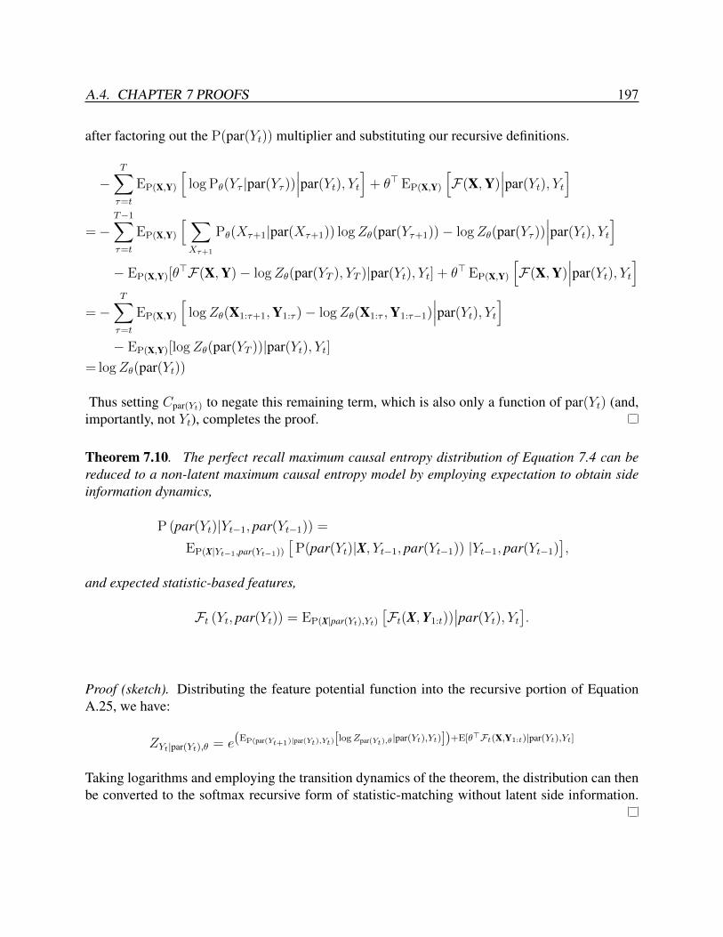
A.4. CHAPTER 7 PROOFS 197
after factoring out the P(par(Yt)) multiplier and substituting our recursive definitions.
−T∑τ=t
EP(X,Y)
[log Pθ(Yτ |par(Yτ ))
∣∣∣par(Yt), Yt]
+ θ> EP(X,Y)
[F(X,Y)
∣∣∣par(Yt), Yt]
=−T−1∑τ=t
EP(X,Y)
[ ∑Xτ+1
Pθ(Xτ+1|par(Xτ+1)) logZθ(par(Yτ+1))− logZθ(par(Yτ ))∣∣∣par(Yt), Yt
]− EP(X,Y)[θ
>F(X,Y)− logZθ(par(YT ), YT )|par(Yt), Yt] + θ> EP(X,Y)
[F(X,Y)
∣∣∣par(Yt), Yt]
=−T∑τ=t
EP(X,Y)
[logZθ(X1:τ+1,Y1:τ )− logZθ(X1:τ ,Y1:τ−1)
∣∣∣par(Yt), Yt]
− EP(X,Y)[logZθ(par(YT ))|par(Yt), Yt]= logZθ(par(Yt))
Thus setting Cpar(Yt) to negate this remaining term, which is also only a function of par(Yt) (and,importantly, not Yt), completes the proof.
Theorem 7.10. The perfect recall maximum causal entropy distribution of Equation 7.4 can bereduced to a non-latent maximum causal entropy model by employing expectation to obtain sideinformation dynamics,
P (par(Yt)|Yt−1, par(Yt−1)) =
EP(X|Yt−1,par(Yt−1))
[P(par(Yt)|X, Yt−1, par(Yt−1)) |Yt−1, par(Yt−1)
],
and expected statistic-based features,
Ft (Yt, par(Yt)) = EP(X|par(Yt),Yt)[Ft(X,Y1:t))
∣∣par(Yt), Yt].
Proof (sketch). Distributing the feature potential function into the recursive portion of EquationA.25, we have:
ZYt|par(Yt),θ = e(EP(par(Yt+1)|par(Yt),Yt)[logZpar(Yt),θ|par(Yt),Yt)])+E[θ>Ft(X,Y1:t)|par(Yt),Yt]
Taking logarithms and employing the transition dynamics of the theorem, the distribution can thenbe converted to the softmax recursive form of statistic-matching without latent side information.

198 APPENDIX A. PROOFS
A.5 Chapter 8 Proofs
Theorem 8.8. A LP/CP formulation of CE for Markov games is possible by considering as vari-ables the entire sequence of joint player actions for the sequence of revealed states, η(A1:T
1:N |S1:T ),and employing appropriate inequality constraints (deviation regret guarantees) and equality con-straints (forcing the strategy over sequences to factor into products of Markovian strategies) onmarginal distributions using linear function of η(A1:T
1:N |S1:T ) variables.
Proof. We consider optimizing over variables that represent the probability of an entire sequenceof actions given the entire sequence of S states, denoted as conditional strategy sequence variables:η(a1:T
1:N |s1:T ). Given the state dynamics P(st+1|st, at), action-state strategy probabilities, π(at|st:T ),can be obtained by marginalizing over a linear function of conditional sequence variables:
π(at1:N |st:T ) =∑s1:t−1
∑a1:t−11:N
∑at+1:T1:N
η(a1:T1:N |s1:T )
t−1∏τ=1
P(sτ |aτ−1, sτ−1)
=∑s1:t−1
∑a1:t−11:N
∑at+1:T1:N
P(a1:T1:N , s
1:t−1|st:T ). (A.29)
Crucially, to match the Markov game setting, the conditional distribution of actions at time step tshould be equivalent regardless of future state variables, st+1:T , since those variables are not yetknown in the Markov game:
∀t,st+1:T ,st+1:Tπ(at1:N |st, st+1:T ) = π(at1:N |st, st+1:T ). (A.30)
We note that the constraints of Equation A.30 are linear functions of conditional strategy sequencevariables via the steps of Equation A.29.

A.5. CHAPTER 8 PROOFS 199
argmax{η(a1:T1:N |s1:T )}
f0({η(a1:T1:N |s1:T )}) (A.31)
such that: ∀t,i,st,ati,ati ′∑
at−i,at+1:T1:N ,s1:t−1,st+1:T
η(a1:T1:N |s1:T )
∏Tτ=1 P(sτ+1|sτ , aτ )P(st+1|st, at)
×
(P(st+1|st, at1:N
′)
(∑τ>t
Utility(sτ , aτ1:N) + Utility(st, at1:N′)
)
− P(st+1|st, at1:N)
(∑τ>t
Utility(sτ , aτ1:N) + Utility(st, at1:N)
))≤ 0
∀t,st,at1:N∑s1:t−1
∑a1:t−11:N
∑at+1:T1:N
η(a1:T1:N |s1:T )
t−1∏τ=1
P(sτ |aτ−1, sτ−1) ≥ 0
∀t,st∑s1:t−1
∑a1:t1:N
∑at+1:T1:N
η(a1:T1:N |s1:T )
t−1∏τ=1
P(sτ |aτ−1, sτ−1) = 1
∀t,st+1:T ,st+1:T
∑s1:t−1
∑a1:t−11:N
∑at+1:T1:N
t−1∏τ=1
P(sτ |aτ−1, sτ−1)(η(a1:T
1:N |s1:T)
(A.32)
− η(a1:T
1:N |s1:t, st+1:T) )
= 0
All constraints are linear in conditional variables, so when −f0 is a linear or convex function, theoptimization (Equation A.31) is a linear program or convex program. We note that the number ofconstraints in the last set of constraints (Equation A.32) can be reduced from O(|S|2T ) to O(|S|T )by chains of equality constraints (rather than all pair-wise constraints). However, the total numberof constraints is still exponential in T and there are a total of O(|S|T |A|NT ) variables in thisformulation.
Theorem 8.10. Given an MCECE strategy profile, no player may decrease the predictability ofher action sequence without creating deviation regret for herself.
Proof. Ignoring all the deviation regret constraints in our notation, consider the decomposition ofthe causally conditioned entropy using the chain rule:
argmax{π(at1:N |st)}
H(AT1:N ||ST ) = argmax{π(at1:N |st)}
(H(ATi ||ST ) +H(AT−i||ST )
)={πMCECE(at−i|st)
}∪ argmax{π(ati|st)}
H(ATi ||ST , AT−i).

200 APPENDIX A. PROOFS
As shown, this can equivalently be viewed as a causally conditioned entropy maximization ofplayer i’s strategy profile (with the suppressed deviation regret constraints) given the combinedMCECE strategy profile of the other players. By definition this is already the least predictablestrategy profile that player i can employ (subject to any deviation regret constraints).
Theorem 8.11. The MCECE solution strategy profile, πMCECE minimizes the worst-case log pre-diction loss for the sequences of joint actions, i.e.,
infP(AT ||ST )
supP(AT ||ST )
∑A,S
P(A,S) log P(AT ||ST ), (A.33)
of all the CE satisfying deviation regret constraints, where P(AT ||ST ) is the (worst possible forprediction) empirical CE strategy and the joint, P(A,S), is the distribution of states and actionsunder that strategy profile and the known state transition dynamics.
Proof. As a special case of Grunwald & Dawid (2003), the causal entropy can be expressed as:H(P(AT ||ST )) = infP(AT ||ST ) EP(A,S)[− log P(AT ||ST )]. Choosing P(YT ||XT ) that maximizes thisthen: supP(AT ||ST ) infP(AT ||ST ) EP(A,S)[− log P(AT ||ST )], which is invariant to swapping the orderof the sup and inf operations.
Lemma 8.14. The MCECE strategy profile for a Markov game is also Markovian.
Proof sketch. The Markovian state transition dynamics of the Markov game imply that the entropyof future actions due to those state dynamics is conditionally independent of past states and ac-tions given the current state of the game. As a consequence, any strategy profile based on certainprevious states and actions can be employed from the current state by pretending those previousstates and actions occurred, and the result is the same amount of entropy (and satisfaction of alldeviation regret constraints) as if those previous states and actions had actually occurred. Thus bymaximization and uniqueness of MCECE strategy profile, all MCECE strategies from the currentstate forward must employ the same (history-dependent) strategy profile, effectively making thatstrategy profile Markovian.
Theorem 8.15. The MCECE strategy profile, πMCECEλ (at1:N |st), has the following recursive form
(with λ ≥ 0):
πMCECEλ (at1:N |st) ∝ e
−(∑
i,ati′ λi,st,ati,a
ti′ ExpectDevGainπ
MCECEi (at1:N ,st,ati
′))
+ExpectEnt(at1:N ,st), (A.34)
where ExpectEnt(at1:N , st) , Eat+1
1:N ,st+1
[ExpectEnt(at+1
1:N , st+1) +H(at+1
1:N |st+1)∣∣at1:N , s
t].
Proof sketch. We find the form of the probability distribution by finding the optimal point of theLagrangian. We suppress the probabilistic positivity constraints and normalization constraints withthe understanding that the resulting probability distribution must normalize to 1.

A.5. CHAPTER 8 PROOFS 201
argmaxπ
H(AT ||ST ) (A.35)
such that: ∀t,i,ati,ati ′,s1:t,a1:t−11:N
ExpectRegretπi (ati, ati′, s1:t, a1:t−1
1:N ) ≤ 0
and probabilistic constraints on π.
The Lagrangian for the optimization of Equation A.35 when using entire history-dependentprobability distributions and parameters is:
Λ(π, λ) = H(a1:T1:N ||s1:T )−
∑t,i,ati,a
ti′,s1:t,a1:t−1
1:N
λt,i,ati,ati′,s1:t,a1:t−1
1:NExpectRegretπi (ati, a
ti′, s1:t, a1:t−1
1:N ) (A.36)
Taking the partial derivative with respect to a history-dependent action probability for a particularstate, we have:
∂Λ(π, λ)
∂ P(at1:N |s1:t, a1:t−11:N )
= −∑
st+1:T ,at+1:T1:N
P(st+1:T , at+1:T ) logT∏τ=t
P(aτ1:N |s1:τ , a1:τ−11:N )
−∑i,ati′
λt,i,ati,ati′,s1:t,a1:t−1
1:NExpectDevGainπi (ati, a
ti′, s1:t, a1:t−1
1:N )
= − log P(at1:N |s1:t, a1:t−11:N )−
∑st+1:T ,at+1:T
1:N
P(st+1:T , at+1:T ) logT∏τ=t
P(aτ1:N |s1:τ , a1:τ−11:N )
−∑i,ati′
λt,i,ati,ati′,s1:t,a1:t−1
1:NExpectDevGainπi (ati, a
ti′, s1:t, a1:t−1
1:N ). (A.37)
Equating Equation A.37 to zero provides the form of the history dependent distribution:
P(at1:N |s1:t, a1:t−11:N ) ∝ exp
{ ∑st+1:T ,at+1:T
1:N
P(st+1:T , at+1:T ) logT∏τ=t
P(aτ1:N |s1:τ , a1:τ−11:N ) (A.38)
−∑i,ati′
λt,i,ati,ati′,s1:t,a1:t−1
1:NExpectDevGainπi (ati, a
ti′, s1:t, a1:t−1
1:N )}.
It is important to note that duality in this optimization relies on a feasible solution on the relativeinterior of the constraint set. This can be accomplished by adding an infinitesimally small amountof slack, ε, to the constraint set Ortiz et al. (2007).
Following the argument that the MCECE is Markovian (Lemma 8.14), Equation A.38 reducesto the Markovian form of the theorem.

202 APPENDIX A. PROOFS
A.6 Chapter 9 ProofsTheorem 9.1. The expected action visitation frequencies, Dax,y , for origin A and goal state Bin the deterministic dynamics maximum causal entropy statistic-matching model can be computedfrom partition functions using the following equation:
Dax,y =ZA→x e−cost(ax,y) Zy→B
ZA→B(A.39)
Proof. Our proof relies on employing the partition function excluding a particular action, which wedenote ZA→B/ax→y =
∑ζA→B :ax,y /∈ζA→B e
−cost(ζ), the partition function restricted to contain a par-ticular action, which we denote ZA→B3ax→y =
∑ζA→B :ax,y∈ζA→B e
−cost(ζ), and two mathematicalseries formulas:
∞∑i=0
xi =1
1− x(A.40)
∞∑i=1
ixi =x
(1− x)2(A.41)
We can combine these ideas by expressing Zy→y3ax,y as the combination of independently cho-sen paths to state x and actions ax,y. First, we note a useful relationship between action inclusivepartition functions and unconstrained partition functions (Equation A.42). We re-express this par-tition function as a sum of increasingly repeated cycles from y to x and containing action ax,y. Wefinally employ our mathematical series formula (Equation A.40) to obtain Equation A.43.
Zy→y3ax,y = e−cost(ax,y)Zx→y = e−cost(ax,y)Zy→x (A.42)
=∞∑k=1
(e−cost(ax,y)Zy→x/ax,y
)k=
1
1− e−cost(ax,y)Zy→x/ax,y− 1 (A.43)
We can express the regular partition function using the action excluding and action containingpartition functions. We can simply combine the partition function for all paths that do not includeax,y with the partition function for all possible paths that do contain ax,y (by taking action ax,y andthen returning to Sx). This value can then be expressed in terms of the action inclusion partitionfunction as shown in Equation A.45 by employing Equation A.42
ZA→x = ZA→x/ax,y + ZA→x/ax,y e−cost(ax,y) Zy→x (A.44)
= ZA→x/ax,y(1 + Zy→y3ax,y
)(A.45)

A.6. CHAPTER 9 PROOFS 203
We count the unnormalized probability mass of paths weighted by action membership by com-bining the mass of different disjoint sets of paths. A valid path from A to B containing action ax,ycan be characterized as:
• A sub-path from A to x that does not include ax,y
• Action ax,y
• Any number of “looping” paths from y to x followed by action ax,y
• A sub-path from y to B that does not include ax,y
Using this construction, the unnormalized probability mass of paths that take action ax→y ex-actly k ≥ 1 times is:
∑ζA→B :#ax,y∈ζ=k
eθ>fζ = ZA→x/ax,ye
−cost(ax,y)(Zy→x/ax,ye
−cost(ax,y))k−1
Zy→B/ax,y (A.46)
The expected action visitation frequencies can then be calculated by combining these unnor-malized probability masses and weighting by the number of actions ax,y contained in each set.
Dax,y =
∑∞k=1 k ZA→x/ax,y e
−cost(ax,y)(Zy→x/ax,ye
−cost(ax,y))k−1
Zy→B/ax,yZA→B
(A.47)
=ZA→x/ax,y e
−cost(ax,y) Zy→B/ax,y
(1 +
∑∞k=1 k
(Zy→x/ax,ye
−cost(ax,y))k)
ZA→B
=
ZA→x/ax,y e−cost(ax,y) Zy→B/ax,y
(1 +
Zy→x/ax,y e−cost(ax,y)
(1−Zy→x/ax,y e−cost(ax,y))2
)ZA→B
(A.48)
=ZA→x/ax,y e
−cost(ax,y) Zy→B/ax,y + ZA→x e−cost(ax,y) Zy→B (1 + Zy→x/ax,y e
−cost(ax,y))
ZA→B
=ZA→x e
−cost(ax,y) Zy→BZA→B
(A.49)
We reduce Equation A.47 to Equation A.48 using the mathematical series formula (EquationA.41) and Equations A.43 and A.42. We reduce Equation A.48 by expanding the product andapplying Equations A.45. Finally, we obtain Equation A.49 using the same logic as employed forEquation A.44.

204 APPENDIX A. PROOFS
Theorem 9.2. For matrix A, if limt→∞ At = 0, then∑∞
t=0 At = (I− A)−1, where I is the identitymatrix and A0 = I.
Proof sketch. If limt→∞At = 0, then by definition:
∞∑t=0
At = I + A∞∑t=0
At (A.50)
∞∑t=0
At(I− A) = I (A.51)
∞∑t=0
At = (I− A)−1, (A.52)
by following simple matrix algebra.
Theorem 9.5. In a discounted future rewards setting with a bounded instantaneous reward andbounded number of actions, the partition functions of the maximum causal entropy model withfinite rewards are guaranteed to converge.
Proof sketch. With discount rate γ, Equation 6.5 can be re-expressed as:
Qsoftθ (at, st) = γEP(st+1|st,at)
[softmax
atQsoftθ (at+1, st+1)|st, at
]+ θ>fst,at (A.53)
For non-convergence to occur, the sum of Qt values at time step t must grow larger than the sumof Qt+∆t values at time step t + ∆t and approaches infinity as t → ∞. However, as these sumsapproach infinity, the loss from discount of the sum which bounds the previous timestep’s partitionmass due to the future, (1−γ)∆t
∑a,sQ
softθ (a, s), must also grow larger than
∑s,a θ
>fs,a, preventinggrowth to infinity (and non-convergence).
A.7 Chapter 11 Proofs
Theorem 11.1. The posterior distribution of goals can be obtained from the log partition func-tions, Vsx→sy , as follows:
P(G|a1:t, s1:t) ∝ P(G) eVst→G − Vs1→G . (A.54)

A.7. CHAPTER 11 PROOFS 205
Proof.
P(G|a1:t, s1:t) ∝ P(a1:t, s1:t|G) P(G)
=∑
at+1:T ,st+1:T
P(a1:T , s1:T |G) P(G)
=
∑at+1:T ,st+1:T
ereward(a1:T ,s1:T )∑a1:T ,s1:T e
reward(a1:T ,s1:T )P(G)
∝ Zst→GZs1→G
P(G)
= P(G) eVst→G−Vs1→G
Theorem 11.2. Action visitation calculations using final reward values as follows:
φ(G) = log P(G|a1:t, s1:t)
= Vst→G − Vs1→G + log P(G),
are equivalent to the goal-probability-weighted visitation calculations:
Dsx|s1:t,a1:t =∑
st+1:T ,at+1:T
(T∑
τ=t+1
I(sx = sτ )
)P(at+1:T , st+1:T |a1:t, s1:t)
of Equation 11.4.
Proof sketch. Writing out the visitation frequencies from state st to goals with potentials weightedby φ(G), we have:
Dsx|φ(G) =Zst→sx
∑G Zsx→G P(G|a1:t, s1:t)∑
G Zst→G P(G|a1:t, s1:t), (A.55)
which is equivalent to the goal-probability-weighted visitation calculation of the theorem.

Bibliography
P. Abbeel, A. Coates, M. Quigley, & A. Y. Ng. An application of reinforcement learning to aero-batic helicopter flight. In NIPS, pages 1–8, 2007. 14.3, 14.3.1
P. Abbeel & A. Y. Ng. Apprenticeship learning via inverse reinforcement learning. In Proc. ICML,pages 1–8, 2004. 1.1, 3.2.2, 3.2.2, 6.6, 6.2.1, 14.3, A.3
P. Ardis & C. Brown. Using conditional random fields for decision-theoretic planning. In ModelingDecisions for Artificial Intelligence, 2009. 3.1, 3.1.2, 3.1.2, 3.4.1, 3.4.2
B. Argall, S. Chernova, M. Veloso, & B. Browning. A survey of robot learning from demonstration.Robotics and Autonomous Systems, 57(5):469–483, 2009. 3, 6.2
H. Attias. Planning by probabilistic inference. In Proc. of the 9th Int. Workshop on ArtificialIntelligence and Statistics, 2003. 3.1
R. Aumann. Subjectivity and correlation in randomized strategies. Journal of Mathematical Eco-nomics, 1(1):67–96, 1974. 8, 8.5
J. Bagnell. Learning decisions: Robustness, uncertainty, and approximation. PhD thesis, CarnegieMellon University, 2004. 3.2.6
C. Baker, J. Tenenbaum, & R. Saxe. Bayesian models of human action understanding. Advancesin Neural Information Processing Systems, 18:99, 2006. 3.2.5
C. Baker, J. Tenenbaum, & R. Saxe. Goal inference as inverse planning. In Proc. of the cognitivescience society, 2007. 3.2.5, 11.3
L. Bao & S. Intille. Activity recognition from user-annotated acceleration data. Pervasive Com-puting, pages 1–17, 2004. 3.1
R. Bellman. A Markovian decision process. Journal of Mathematics and Mechanics, 6:679–684,1957. 2.2.1, 2.2.1, 4.2.5, 6.1.1, 6.2.2, 6.3.2, 9.1, 9.3.1
M. Ben-Akiva. Structure of passenger travel demand models. 1974. 3.3.3
206

BIBLIOGRAPHY 207
M. Bennewitz, W. Burgard, & S. Thrun. Learning motion patterns of persons for mobile servicerobots. In Proc. ICRA, pages 3601–3606, 2002. 13.1
S. Boyd, L. El Ghaoui, E. Feron, & V. Balakrishnan. Linear matrix inequalities in system andcontrol theory. SIAM, 15, 1994. 3.2.1
S. Boyd & L. Vandenberghe. Convex Optimization. Cambridge University Press, March 2004.5.2.1, A.2
S. Boyd, L. Xiao, & A. Mutapcic. Subgradient methods. Lecture notes of EE392o, StanfordUniversity, Autumn Quarter, 2003. 10.2.3
S. Brin & L. Page. The anatomy of a large-scale hypertextual Web search engine* 1. Computernetworks and ISDN systems, 30(1-7):107–117, 1998. 9.1.2
C. Broyden. The convergence of a class of double-rank minimization algorithms 1. general con-siderations. IMA Journal of Applied Mathematics, 6(1):76, 1970. 10.2.4
H. Bui, S. Venkatesh, & G. West. Policy recognition in the abstract hidden Markov model. Journalof Artificial Intelligence Research, 17(1):451–499, 2002. 3.1.1
U. Chajewska, D. Koller, & D. Ormoneit. Learning an agent’s utility function by observing behav-ior. In In Proc. of the 18th Intl Conf. on Machine Learning, pages 35–42, 2001. 3.2.1
G. Cooper. A method for using belief networks as influence diagrams. In Workshop on Uncertaintyin Artificial Intelligence, pages 55–63, 1988. 3.1
D. Coppersmith & S. Winograd. Matrix multiplication via arithmetic progressions. Journal ofsymbolic computation, 9(3):251–280, 1990. 9.1.2
M. Costa-Gomes, V. Crawford, & B. Broseta. Cognition and behavior in normal-form games: Anexperimental study. Econometrica, 69(5):1193–1235, 2001. 15.2
T. Cover & J. Thomas. Elements of information theory. John Wiley and sons, 2006. 4.1, 4.1.3,4.16, 4.17, 8.2.2
M. da Silva, F. Durand, & J. Popovic. Linear Bellman combination for control of character anima-tion. ACM Transactions on Graphics (TOG), 28(3):1–10, 2009. 3.2.6
E. W. Dijkstra. A note on two problems in connexion with graphs. Numerische Mathematik, 1:269–271, 1959. 13.2.1
A. Drake. Observation of a Markov process through a noisy channel. PhD thesis, MassachusettsInstitute of Technology, 1962. 2.2.1

208 BIBLIOGRAPHY
M. Dudık & G. Gordon. A sampling-based approach to computing equilibria in succinct extensive-form games. In Proc. 25th Conference on Uncertainty in Artificial Intelligence. Citeseer, 2009.8.3
M. Dudık & R. E. Schapire. Maximum entropy distribution estimation with generalized regular-ization. In Proc. COLT, pages 123–138, 2006. 5.1.4, 5.1
E. Feinberg & A. Shwartz. Handbook of Markov Decision Process Methods and Applications.Kluwer Academic Publishers, 2002. 2.8, 2.2.1
D. Ferguson & A. T. Stentz. Field D*: An interpolation-based path planner and replanner. In Proc.ISRR, pages 239–253, 2005. 13.2.1
J. Filar, K. Vrieze, & O. Vrieze. Competitive Markov decision processes. Springer Verlag, 1997.8.2, 8.2
R. Fletcher. A new approach to variable metric algorithms. The Computer Journal, 13(3):317,1970. 10.2.4
A. F. Foka & P. E. Trahanias. Predictive autonomous robot navigation. In Proc. IROS, pages490–495, 2002. 13.1
N. Gaarder & J. Wolf. The capacity region of a multiple-access discrete memoryless channel canincrease with feedback (corresp.). Information Theory, IEEE Transactions on, 21(1):100–102,1975. 4.2.5
A. Galata, N. Johnson, & D. Hogg. Learning variable length Markov models of behaviour. Com-puter Vision and Image Understanding (CVIU) Journal, 2001. 3.1.1, 13.1, 13.3.5
A. Giffin & A. Caticha. Updating probabilities with data and moments. In Bayesian Inference andMaximum Entropy Methods in Science and Engineering, volume 954, pages 74–84, 2007. 5.1.4
I. Gilboa & E. Zemel. Nash and correlated equilibria: Some complexity considerations. Gamesand Economic Behavior, 1(1):80–93, 1989. 8.1.2
D. Goldfarb. A family of variable metric updates derived by variational means. Mathematics ofComputing, 24(109):23–26, 1970. 10.2.4
Google 2008. Google maps, April 2008. URL http://maps.google.com/. 12.2
A. Greenwald & Hall. Correlated Q-learning. In Proc. ICML, pages 242–249, 2003. 8.6, 8.1.2
P. D. Grunwald & A. P. Dawid. Game theory, maximum entropy, minimum discrepancy, and robustbayesian decision theory. Annals of Statistics, 32:1367–1433, 2003. 5.2, 5.2.3, 8.11, A.2, A.5

BIBLIOGRAPHY 209
P. Hart, N. Nilsson, & B. Raphael. A formal basis for the heuristic determination of minimum costpaths. IEEE Transactions on Systems Science and Cybernetics, 4:100–107, 1968. 9.1.4
S. Hart & A. Mas-Colell. A simple adaptive procedure leading to correlated equilibrium. Econo-metrica, 68(5):1127–1150, 2000. 8.2
D. Heckerman, J. S. Breese, & K. Rommelse. Troubleshooting under uncertainty. In Communica-tions of the ACM, pages 121–130, 1994. 14.2.2
P. Henry, C. Vollmer, B. Ferris, & D. Fox. Learning to Navigate Through Crowded Environments.In Proc. ICRA, 2010. 13.4
R. Howard. Information value theory. IEEE Transactions on systems science and cybernetics, 2(1):22–26, 1966. 6.4
R. A. Howard & J. E. Matheson. Influence diagrams. In Readings on the Principles and Appli-cations of Decision Analysis, pages 721–762. Strategic Decisions Group, 1984. 2.2.3, 2.2.3,7
B. Hull, V. Bychkovsky, Y. Zhang, K. Chen, M. Goraczko, A. K. Miu, E. Shih, H. Balakrishnan,& S. Madden. CarTel: A Distributed Mobile Sensor Computing System. In ACM SenSys, pages125–138, 2006. 12.6.2
E. Jaynes. The relation of Bayesian and maximum entropy methods. Maximum-entropy andBayesian methods in science and engineering, 1, 1988. 5.1.4
E. Jaynes & G. Bretthorst. Probability theory: the logic of science. Cambridge Univ Pr, 2003.5.1.1
E. T. Jaynes. Information theory and statistical mechanics. Physical Review, 106:620–630, 1957.1.1, 1.5, 5, 5.1, 5.1.1, 8.7
F. Jensen, F. Jensen, S. Dittmer, et al. From influence diagrams to junction trees. In Proceedingsof the Tenth Conference on Uncertainty in Artificial Intelligence, 1994. 3.1
R. Kalman. A new approach to linear filtering and prediction problems. Journal of basic Engi-neering, 82(1):35–45, 1960. 1
R. Kalman. When is a linear control system optimal? Trans. ASME, J. Basic Engrg., 86:51–60,1964. 3.2.1
R. E. Kalman & R. S. Bucy. New results in linear filtering and prediction theory. AMSE Journ.Basic Eng., pages 95–108, 1962. 13.1
210 BIBLIOGRAPHY
B. Kappen, V. Gomez, M. Opper, & T. Berlin. Optimal control as a graphical model inferenceproblem. (In submission), 2010. 3.1
H. Kappen. Linear theory for control of nonlinear stochastic systems. Physical review letters, 95(20):200201, 2005. 3.2.6
R. Kindermann, J. Snell, & A. M. Society. Markov random fields and their applications. AmericanMathematical Society Providence, Rhode Island, 1980. 2.1.2
J. Kivinen & M. Warmuth. Exponentiated gradient versus gradient descent for linear predictors.Information and Computation, 132(1):1–63, 1997. 10.2.2
G. Kramer. Directed Information for Channels with Feedback. PhD thesis, Swiss Federal Instituteof Technology (ETH) Zurich, 1998. 4.2.2, 4.18, 4.19, 4.2.5, 4.26, 4.2.5, 5.3.1, 8.2.1
A. Krause & C. Guestrin. Optimal nonmyopic value of information in graphical models-efficientalgorithms and theoretical limits. In International Joint Conference on Artificial Intelligence,volume 19, page 1339. Citeseer, 2005. 6.4
D. Krishnamurthy & E. Todorov. Inverse Optimal Control with Linearly-solvable MDPs. In ICML,2010. 3.2.6, 3.4.2
J. Krumm. A Markov model for driver route prediction. Society of Automative Engineers (SAE)World Congress, 2008. 3, 12.6.1
J. Krumm & E. Horvitz. Predestination: Inferring destinations from partial trajectories. In Proc.Ubicomp, pages 243–260, 2006. 12.6.3
S. Kullback & R. A. Leibler. On information and sufficiency. Annals of Mathematical Statistics,22:49–86, 1951. 4.1.1
S. Kumar & M. Hebert. Discriminative random fields. Int. J. Comput. Vision, 68(2):179–201,2006. ISSN 0920-5691. 2.1.2, 3.1.2
J. Lafferty, A. McCallum, & F. Pereira. Conditional random fields: Probabilistic models for seg-menting and labeling sequence data. In Proc. ICML, pages 282–289, 2001. 1.1, 2.1.2, 2.1.2,3.1.2, 5.3.4, 6, 6.2.5, 6.2.5
C. Lemke & J. Howson Jr. Equilibrium points of bimatrix games. Journal of the Society forIndustrial and Applied Mathematics, 12(2):413–423, 1964. 8.1.2
J. Letchner, J. Krumm, & E. Horvitz. Trip router with individualized preferences (trip): Incorpo-rating personalization into route planning. In Proc. IAAI, pages 1795–1800, 2006. 12.2, 12.6.2

BIBLIOGRAPHY 211
L. Liao, D. Fox, & H. Kautz. Extracting places and avctivities from GPS traces using hierarchicalconditional random fields. Int. J. Rob. Res., 26(1):119–134, 2007a. ISSN 0278-3649. 2.1.2,3.1.2
L. Liao, D. J. Patterson, D. Fox, & H. Kautz. Learning and inferring transportation routines.Artificial Intelligence, 171(5-6):311–331, 2007b. ISSN 0004-3702. 12.6.1
R. Luce. Individual choice behavior. Wiley New York, 1959. 3.3.1
L. MacDermed & C. L. Isbell. Solving Stochastic Games. In Proc. NIPS, 2009. 8.3.2
R. MacLachlan. Tracking moving objects from a moving vehicle using a laser scanner. Techni-cal Report CMU-RI-TR-05-07, Robotics Institute, Carnegie Mellon University, Pittsburgh, PA,2005. 13.3.1
R. Madhavan & C. Schlenoff. Moving object prediction for off-road autonomous navigation. InSPIE Aerosense Conference, 2003. 13.1
MapPoint 2008. Microsoft mappoint, April 2008. URL http://www.microsoft.com/mappoint/. 12.2
MapQuest 2008. Mapquest, April 2008. URL http://www.mapquest.com/. 12.2
H. Marko. The bidirectional communication theory – a generalization of information theory. InIEEE Transactions on Communications, pages 1345–1351, 1973. 4.2.2
J. L. Massey. Causality, feedback and directed information. In Proc. IEEE International Sympo-sium on Information Theory and Its Applications, pages 27–30, 1990. 4.2.2, 4.23, 4.24, 4.2.5,4.25, 4.2.5
D. McFadden. Conditional logit analysis of qualitative choice behavior. Frontiers in Econometrics,pages 105–142, 1974. 3.3.1, 3.3.2, 3.4.1, 3.4.2
R. McKelvey & T. Palfrey. An experimental study of the centipede game. Econometrica: Journalof the Econometric Society, 60(4):803–836, 1992. 15.2
R. McKelvey & T. Palfrey. Quantal response equilibria for normal form games. Games andEconomic Behavior, 10(1):6–38, 1995. 15.1
R. McKelvey & T. Palfrey. Quantal response equilibria for extensive form games. ExperimentalEconomics, 1(1):9–41, 1998. 15.1
C. Mertz. A 2d collision warning framework based on a Monte Carlo approach. In Proc. ofIntelligent Transportation Systems, 2004. 13.1

212 BIBLIOGRAPHY
A. C. Miller, M. M. Merkhofer, R. A. Howard, J. E. Matheson, & T. R. Rice. Development ofautomated aids for decision analysis. Technical report, 1976. 2.2.3, 7
K. Murphy. Dynamic Bayesian Networks: Representation, Inference and Learning. PhD thesis,UNIVERSITY OF CALIFORNIA, 2002. 2.2
C. Murray & G. Gordon. Multi-robot negotiation: approximating the set of subgame perfectequilibria in general-sum stochastic games. In Proc. NIPS, pages 1001–1008, 2007. 8.3.2
J. Nash. Non-cooperative games. Annals of mathematics, 54(2):286–295, 1951. 8, 8.1.2, 8.1.2,8.1.2
Y. Nesterov & A. Nemirovski. Interior-point polynomial algorithms in convex programming. So-ciety for Industrial Mathematics, 1987. 10.2.4
G. Neu & C. Szepesvari. Apprenticeship learning using inverse reinforcement learning and gradi-ent methods. In Proc. UAI, pages 295–302, 2007. 3.2.5, 3.6, 12.6.2
A. Y. Ng & S. Russell. Algorithms for inverse reinforcement learning. In Proc. ICML, pages663–670, 2000. 1.1, 3.2.1, 3.1, 3.2.1
T. Nielsen & F. Jensen. Learning a decision maker’s utility function from (possibly) inconsistentbehavior. Artificial Intelligence, 160(1-2):53–78, 2004. 3.2.7, 7.4
A. Nilim & L. El Ghaoui. Robust control of Markov decision processes with uncertain transitionmatrices. Operations Research, 53(5):780–798, 2005. 3.2.6
L. E. Ortiz, R. E. Shapire, & S. M. Kakade. Maximum entropy correlated equilibrium. In AISTATS,pages 347–354, 2007. 1.1, 8.7, 8.1.2, 8.2.1, 8.10, A.5
C. Papadimitriou & T. Roughgarden. Computing equilibria in multi-player games. In Proceedingsof the sixteenth annual ACM-SIAM symposium on Discrete algorithms, pages 82–91. Societyfor Industrial and Applied Mathematics, 2005. 8.1.2
J. Pearl. Causality: Models, Reasoning, and Inference. Cambridge University Press, 2000. 4.2.1
H. H. Permuter, Y.-H. Kim, & T. Weissman. On directed information and gambling. In Proc. IEEEInternational Symposium on Information Theory, pages 1403–1407, 2008. 4.19, 4.2.5, 4.2.5,4.27
S. Petti & T. Fraichard. Safe motion planning in dynamic environments. In Proc. IROS, pages3726–3731, 2005. 13.1
K. Poh & E. Horvitz. A graph-theoretic analysis of information value. In Uncertainty in ArtificialIntelligence: Proceedings of the Twelfth Conference, pages 427–435, 1996. 6.4

BIBLIOGRAPHY 213
D. Pomerleau. Alvinn: An autonomous land vehicle in a neural network. In Advances in NeuralInformation Processing Systems 1, 1989. 3.2
M. L. Puterman. Markov Decision Processes: Discrete Stochastic Dynamic Programming. Wiley-Interscience, 1994. 1, 2.2.1, 12.3.1
D. Ramachandran & E. Amir. Bayesian inverse reinforcement learning. In Proc. IJCAI, pages2586–2591, 2007. 3.2.5, 12.6.2
N. Ratliff, J. A. Bagnell, & M. Zinkevich. Maximum margin planning. In Proc. ICML, pages729–736, 2006. 3.2.3, 12.6.2, 14.3, 14.3.2
N. Ratliff, D. Bradley, J. Bagnell, & J. Chestnutt. Boosting structured prediction for imitationlearning. Advances in Neural Information Processing Systems, 19:1153, 2007. 3.2.3
N. Ratliff, B. Ziebart, K. Peterson, J. A. Bagnell, M. Hebert, A. K. Dey, & S. Srinivasa. Inverseoptimal heuristic control for imitation learning. In Proc. AISTATS, pages 424–431, 2009. 1.7
H. Robbins & S. Monro. A stochastic approximation method. The Annals of Mathematical Statis-tics, pages 400–407, 1951. 10.2.2
A. Rosenblueth, N. Wiener, & J. Bigelow. Behavior, purpose and teleology. Philosophy of Science,10(1):18–24, 1943. 1.2, 1.3, 1.3, 1.3, 1.3
C. Schlenoff, R. Madhavan, & T. Barbera. A hierarchical, multi-resolutional moving object pre-diction approach for autonomous on-road driving. Proc. ICRA, 2:1956–1961, 2004. ISSN1050-4729. 13.1
R. Shachter. Evaluating influence diagrams. Operations Research, 34(6):871–882, 1986. 2.2.3
R. Shachter. Model building with belief networks and influence diagrams. 2007. 2.2
R. Shachter & M. Peot. Decision making using probabilistic inference methods. In Uncertainty inArtificial Intelligence, pages 276–283, 1992. 2.2.3, 3.1
D. Shanno. Conditioning of quasi-Newton methods for function minimization. Mathematics ofComputation, 24(111):647–656, 1970. 10.2.4
C. Shannon. The zero error capacity of a noisy channel. Information Theory, IRE Transactions on,2(3):8–19, 1956. 4.2.5
C. Shannon. Two-way communication channels. In Proc. 4th Berkeley Symp. Math. Stat. Prob,volume 1, pages 351–384, 1961. 4.2.5
C. E. Shannon. A mathematical theory of communication. Bell system technical journal, 27, 1948.4

214 BIBLIOGRAPHY
N. Shor, K. Kiwiel, & A. Ruszcayski. Minimization methods for non-differentiable functions.Springer-Verlag New York, Inc. New York, NY, USA, 1985. 10.2.3
R. Simmons, B. Browning, Y. Zhang, & V. Sadekar. Learning to predict driver route and destinationintent. Proc. Intelligent Transportation Systems Conference, pages 127–132, 2006. 3, 12.6.1,12.6.2
D. Stahl & P. Wilson. On Players Models of Other Players: Theory and Experimental Evidence.Games and Economic Behavior, 10(1):218–254, 1995. 15.2
A. Steinfeld, D. Manes, P. Green, & D. Hunter. Destination entry and retrieval with the ali-scoutnavigation system. The University of Michigan Transportation Research Institute No. UMTRI-96-30, 1996. 12.1, 12.6.3
R. J. Sternberg & W. Salter. Handbook of Human Intelligence. Cambridge University Press, 1982.1, 1.3
U. Syed, M. Bowling, & R. E. Schapire. Apprenticeship learning using linear programming. InICML ’08: Proceedings of the 25th international conference on Machine learning, pages 1032–1039, 2008. 3.2.2, 3.2.4
U. Syed & R. Schapire. A game-theoretic approach to apprenticeship learning. In Advances inNeural Information Processing Systems 20, pages 1449–1456. 2007. 3.2.4, 3.5
S. Tadokoro, M. Hayashi, Y. Manabe, Y. Nakami, & T. Takamori. On motion planning of mobilerobots which coexist and cooperate with human. In Proc. IROS, pages 518–523, 1995. 13, 13.1
E. M. Tapia, S. S. Intille, & K. Larson. Activity recognition in the home using simple and ubiqui-tous sensors. In Proc. Pervasive, pages 158–175, 2004. 3.1.1
S. Tatikonda. Control under Communication Constraints. PhD thesis, Massachusetts Institute ofTechnology, 2000. 4.2.5, 4.2.5
R. Taylor. Purposeful and non-purposeful behavior: A rejoinder. Philosophy of Science, 17(4):327–332, 1950. 1.3, 1.1
S. Thrun, W. Burgard, & D. Fox. Probabilistic Robotics (Intelligent Robotics and AutonomousAgents). The MIT Press, September 2005. 12.4.3, 13.1
N. Tishby & D. Polani. Information Theory of Decisions and Actions. 2010. 6.4
E. Todorov. Linearly-solvable Markov decision problems. In NIPS, pages 1369–1376, 2006. 3.2.6,3.4.1, 3.4.2

BIBLIOGRAPHY 215
E. Todorov. Compositionality of optimal control laws. In Advances in Neural Information Pro-cessing Systems, 2009a. 3.2.6, 3.8, 11.3
E. Todorov. Efficient computation of optimal actions. Proceedings of the National Academy ofSciences, 106(28):11478, 2009b. 3.2.6
M. Toussaint. Robot trajectory optimization using approximate inference. In Proceedings of the26th Annual International Conference on Machine Learning. ACM New York, NY, USA, 2009.3.1.2, 3.4.1, 3.4.2, 6.17
M. Toussaint & A. Storkey. Probabilistic inference for solving discrete and continuous stateMarkov Decision Processes. In Proceedings of the 23rd international conference on Machinelearning, page 952. ACM, 2006. 3.1, 3.1.1
K. Tsuda, G. Ratsch, & M. Warmuth. Matrix exponentiated gradient updates for on-line learningand bregman projection. Journal of Machine Learning Research, 6(1):995, 2006. 10.3.1
D. L. Vail, M. M. Veloso, & J. D. Lafferty. Conditional random fields for activity recognition. InProc. AAMAS, pages 1–8, 2007. 2.1.2, 3.1.2
D. A. Vasquez Govea, T. Fraichard, O. Aycard, & C. Laugier. Intentional motion on-line learningand prediction. In Proc. Int. Conf. on Field and Service Robotics, pages 411–425, 2005. 13.1
M. Veloso. Planning and learning by analogical reasoning. Springer, 1994. 3.1.1
D. Verma & R. Rao. Goal-based imitation as probabilistic inference over graphical models. InProc. NIPS, pages 1393–1400, 2006. 3.1.1
S. Vishwanathan, N. Schraudolph, M. Schmidt, & K. Murphy. Accelerated training of condi-tional random fields with stochastic gradient methods. In Proceedings of the 23rd internationalconference on Machine learning, page 976. ACM, 2006. 10.2.2
M. Weiser. The computer for the twenty-first century. Scientific American, 265(3):94–104, 1991.1.2
J. R. Wright & K. Leyton-Brown. Beyond equilibrium: Predicting human behavior in normal-formgames. In Proc. AAAI, 2010. 15.2
Yahoo 2008. Yahoo! maps, April 2008. URL http://maps.yahoo.com/. 12.2
N. Zhang. Probabilistic inference in influence diagrams. Computational Intelligence, 14(4):475–497, 1998. 3.1
B. D. Ziebart, J. A. Bagnell, & A. K. Dey. Probabilistic approaches for robotics and control. InNIPS Workshop: Probabilistic Approaches for Robotics and Control, 2009a. 1.7

216 BIBLIOGRAPHY
B. D. Ziebart, J. A. Bagnell, & A. K. Dey. Maximum Causal Entropy Correlated Equilibria forMarkov Games. In AAAI Worksop: Interactive Decision Theory and Game Theory, 2010a. 1.1,1.7
B. D. Ziebart, J. A. Bagnell, & A. K. Dey. Modeling interaction via the principle of maximumcausal entropy. In ICML, 2010b. 1.1, 1.7, 5, 6
B. D. Ziebart, A. K. Dey, & J. A. Bagnell. Fast planning for dynamic preferences. In Proc. ICAPS,2008a. 1.7
B. D. Ziebart, A. Maas, J. A. Bagnell, & A. K. Dey. Maximum entropy inverse reinforcementlearning. In NIPS Workshop: Robotics Challenges for Machine Learning, 2007. 1.7
B. D. Ziebart, A. Maas, J. A. Bagnell, & A. K. Dey. Maximum entropy inverse reinforcementlearning. In Proc. AAAI, 2008b. 1.1, 1.7, 3.1.2, 3.2.6, 3.4.2
B. D. Ziebart, A. Maas, A. K. Dey, & J. A. Bagnell. Navigate like a cabbie: Probabilistic reasoningfrom observed context-aware behavior. In Proc. Ubicomp, 2008c. 1.7, 3.2.6
B. D. Ziebart, N. Ratliff, G. Gallagher, C. Mertz, K. Peterson, J. A. Bagnell, M. Hebert, A. K. Dey,& S. Srinivasa. Planning-based prediction for pedestrians. In Proc. IROS, 2009b. 1.7
M. Zinkevich, A. Greenwald, & M. Littman. Cyclic equilibria in Markov games. In Proc. NIPS,volume 18, pages 1641–1648, 2006. 8.3.2, 14.1.1


![[PPT]DIRECT, PURPOSEFUL EXPERIENCES AND BEYONDcreativityandinnovations21st.weebly.com/uploads/2/4/3/2/... · Web viewWhy are these direct experiences described to be purposeful? Purposeful](https://static.fdocuments.net/doc/165x107/5b1820407f8b9a28258b78ce/pptdirect-purposeful-experiences-and-beyondcreativi-web-viewwhy-are-these.jpg)