Modeling Pixel Means and CovariancesUsing Factorized Third-Order Boltzmann Machines

Marc’Aurelio Ranzato Geoffrey E. HintonDepartment of Computer Science - University of Toronto

10 King’s College Road, Toronto, Canada{ranzato,hinton}@cs.toronto.edu

Abstract

Learning a generative model of natural images is a use-ful way of extracting features that capture interesting regu-larities. Previous work on learning such models has focusedon methods in which the latent features are used to deter-mine the mean and variance of each pixel independently, oron methods in which the hidden units determine the covari-ance matrix of a zero-mean Gaussian distribution. In thiswork, we propose a probabilistic model that combines thesetwo approaches into a single framework. We represent eachimage using one set of binary latent features that model theimage-specific covariance and a separate set that model themean. We show that this approach provides a probabilis-tic framework for the widely used simple-cell complex-cellarchitecture, it produces very realistic samples of naturalimages and it extracts features that yield state-of-the-artrecognition accuracy on the challenging CIFAR 10 dataset.

1. Introduction

Many computer vision algorithms are based on proba-bilistic models of natural images that are used to providesensible priors for tasks such as denoising, inpainting [28]and segmentation [5]. Models of natural images are alsoused to produce representations capturing features that canbe employed in higher level tasks such as object recogni-tion [10, 32, 14]. Learning good representations of images,as opposed to using engineered descriptors [21, 18, 3], is acrucial step towards building general systems that can easilyadapt to different domains.

Devising models of natural images is challenging be-cause images are continuous, high-dimensional and highlystructured. Recent models have tried to capture high-order dependencies by using hierarchical models that ex-tract highly non-linear representations of the input [13, 15].In particular, deep learning methods construct hierarchies

composed of multiple layers by greedily training each layerseparately using unsupervised algorithms [10, 32, 17, 12].These methods are very appealing because 1) they adaptto the data, 2) they recursively build hierarchies using un-supervised algorithms breaking up the difficult problem oflearning hierarchical non-linear systems into a sequence ofsimpler learning tasks that use only unlabeled data, and 3)they have demonstrated good performance on a variety ofdomains, from handwritten character recognition to genericobject recognition [10, 17, 12]. In this paper we propose anew module for deep learning that is specifically designedto represent natural images well. We start by giving somebackground and motivation for this approach.

1.1. Image Representations

The probabilistic model we are interested in has two setsof random variables, those that are observed and those thatare latent and must be inferred. The former set consists ofthe pixels of an image patch, also called visible units; an ex-ample is given in fig. 1-A. The latter set consists of latent orhidden units that we would like to infer efficiently from theobservation. The most efficient inference is achieved whenthe posterior distribution over the latent variables is facto-rial and simple to compute for each hidden unit, requiringno iterative time-consuming approximation. In order to un-derstand how well the model captures the structure of theobserved image, we can look at how well it reconstructs theimage using the conditional distribution over the pixel val-ues specified by its latent representation.

There are two main approaches. The most popular ap-proach uses the hidden units to predict the mean intensityof each pixel independently from all the others. The con-ditional distribution is typically Gaussian with a mean de-pending on the configuration of the hiddens and a fixeddiagonal covariance matrix. Methods such as sparse cod-ing [22], probabilistic PCA [2], Factor Analysis [8] and theGaussian RBM [4, 10, 1, 17, 16] use this approach. It isconceptually simple but it does not model the strong depen-

1

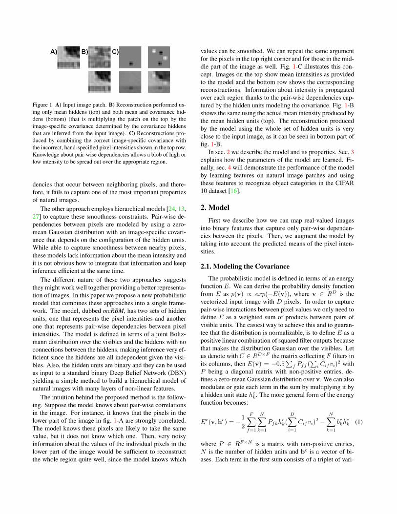
Figure 1. A) Input image patch. B) Reconstruction performed us-ing only mean hiddens (top) and both mean and covariance hid-dens (bottom) (that is multiplying the patch on the top by theimage-specific covariance determined by the covariance hiddensthat are inferred from the input image). C) Reconstructions pro-duced by combining the correct image-specific covariance withthe incorrect, hand-specified pixel intensities shown in the top row.Knowledge about pair-wise dependencies allows a blob of high orlow intensity to be spread out over the appropriate region.

dencies that occur between neighboring pixels, and there-fore, it fails to capture one of the most important propertiesof natural images.

The other approach employs hierarchical models [24, 13,27] to capture these smoothness constraints. Pair-wise de-pendencies between pixels are modeled by using a zero-mean Gaussian distribution with an image-specific covari-ance that depends on the configuration of the hidden units.While able to capture smoothness between nearby pixels,these models lack information about the mean intensity andit is not obvious how to integrate that information and keepinference efficient at the same time.

The different nature of these two approaches suggeststhey might work well together providing a better representa-tion of images. In this paper we propose a new probabilisticmodel that combines these approaches into a single frame-work. The model, dubbed mcRBM, has two sets of hiddenunits, one that represents the pixel intensities and anotherone that represents pair-wise dependencies between pixelintensities. The model is defined in terms of a joint Boltz-mann distribution over the visibles and the hiddens with noconnections between the hiddens, making inference very ef-ficient since the hiddens are all independent given the visi-bles. Also, the hidden units are binary and they can be usedas input to a standard binary Deep Belief Network (DBN)yielding a simple method to build a hierarchical model ofnatural images with many layers of non-linear features.

The intuition behind the proposed method is the follow-ing. Suppose the model knows about pair-wise correlationsin the image. For instance, it knows that the pixels in thelower part of the image in fig. 1-A are strongly correlated.The model knows these pixels are likely to take the samevalue, but it does not know which one. Then, very noisyinformation about the values of the individual pixels in thelower part of the image would be sufficient to reconstructthe whole region quite well, since the model knows which

values can be smoothed. We can repeat the same argumentfor the pixels in the top right corner and for those in the mid-dle part of the image as well. Fig. 1-C illustrates this con-cept. Images on the top show mean intensities as providedto the model and the bottom row shows the correspondingreconstructions. Information about intensity is propagatedover each region thanks to the pair-wise dependencies cap-tured by the hidden units modeling the covariance. Fig. 1-Bshows the same using the actual mean intensity produced bythe mean hidden units (top). The reconstruction producedby the model using the whole set of hidden units is veryclose to the input image, as it can be seen in bottom part offig. 1-B.

In sec. 2 we describe the model and its properties. Sec. 3explains how the parameters of the model are learned. Fi-nally, sec. 4 will demonstrate the performance of the modelby learning features on natural image patches and usingthese features to recognize object categories in the CIFAR10 dataset [16].

2. ModelFirst we describe how we can map real-valued images

into binary features that capture only pair-wise dependen-cies between the pixels. Then, we augment the model bytaking into account the predicted means of the pixel inten-sities.

2.1. Modeling the Covariance

The probabilistic model is defined in terms of an energyfunction E. We can derive the probability density functionfrom E as p(v) ∝ exp(−E(v)), where v ∈ RD is thevectorized input image with D pixels. In order to capturepair-wise interactions between pixel values we only need todefine E as a weighted sum of products between pairs ofvisible units. The easiest way to achieve this and to guaran-tee that the distribution is normalizable, is to define E as apositive linear combination of squared filter outputs becausethat makes the distribution Gaussian over the visibles. Letus denote with C ∈ RD×F the matrix collecting F filters inits columns, then E(v) = −0.5

∑f Pff (

∑i Cifvi)

2 withP being a diagonal matrix with non-positive entries, de-fines a zero-mean Gaussian distribution over v. We can alsomodulate or gate each term in the sum by multiplying it bya hidden unit state hck. The more general form of the energyfunction becomes:

Ec(v,hc) = −12

F∑f=1

N∑k=1

Pfkhck(

D∑i=1

Cifvi)2 −N∑k=1

bckhck (1)

where P ∈ RF×N is a matrix with non-positive entries,N is the number of hidden units and bc is a vector of bi-ases. Each term in the first sum consists of a triplet of vari-

Figure 2. Toy illustration of the model. Factors (the triangles) com-pute the projection of the input image (whose pixels are denotedby vi) with a set of filters (columns of matrix C). Their output issquared because each factor is connected twice to the same imagewith the same set of filters. The square outputs are sent to binaryhidden units after projection with a second layer matrix (matrix P )that pools similar filters. Because the second layer matrix is non-positive the binary hidden units use their “off” states to representabnormalities in the covariance structure of the data.

ables that are multiplied together: two visibles and one hid-den. This is an example of a third-order Boltzmann Ma-chine [29]. A given configuration of the hidden units hc,that we call covariance hiddens, specifies the interaction be-tween pairs of visibles. The number of covariance matricesthat the model can generate is exponential in the numberof hidden units since the representation is binary and dis-tributed. Unlike general higher-order Boltzmann Machines,the interaction between the visibles and the hiddens is fac-torized to reduce the number of parameters. The system canbe represented as in fig. 2 where there are deterministic fac-tors that are connected twice to the image with the same setof filters and once to the hidden units. We call this modelcRBM because it is a Restricted Boltzmann Machine [4] thatmodels the covariance structure of images.

Since the energy adds terms that have only one hiddenunit the conditional distribution over the hiddens is factorial.The conditional distribution over the k-th hidden unit is:

p(hck = 1 | v) = σ(12

F∑f=1

Pfk(D∑i=1

Cifvi)2 + bck) (2)

where σ(x) = 1/(1 + exp(−x)) is the logistic function.The computation required for each hidden unit is consistentwith biologically inspired models of low level vision wherea simple-cell projects the input along a filter, and complex-cells pool many rectified simple cell outputs together toachieve a more invariant representation. The conditionaldistribution over the visibles is a zero-mean Gaussian dis-tribution with an inverse covariance matrix that depends onhc:

Σ−1 = Cdiag(Phc)C ′ (3)

2.2. Modeling Mean and Covariance

In order to take into account the predicted mean intensi-ties of the visible units we add an extra term to the energyfunction: E(v,hc,hm) = Ec(v,hc) +Em(v,hm), whereEc is defined in eq.1, and Em is defined as:

Em(v,hm) = −M∑j=1

D∑i=1

Wijhmj vi −

M∑j=1

bmj hmj (4)

where there are M hidden units hmj , dubbed mean hiddens,with direct connections Wij to the visibles and biases bm.The conditional distribution over the hiddens is:

p(hmj = 1 | v) = σ(D∑i=1

Wijvi + bmj ) (5)

while the conditional distribution over the visibles becomes:

p(v | hc,hm) ∼ N

Σ(M∑j=1

Wijhmj ), Σ

(6)

where Σ is given in eq. 3. The mean of the conditional overthe visibles depends on both covariance and mean hiddenunits, and the conditional over both sets of hiddens remainsfactorial.

We can make the model more robust to large variationsin the contrast of the input image by computing not the innerproduct but the cosine of the angle between input image andfilters. We perform this normalization only in the energyfunction Ec. The overall energy becomes:

E(v,hc,hm) = −12

F∑f=1

N∑k=1

Pfkhck(

D∑i=1

Cif‖Cf‖

vi‖v‖

)2

−N∑k=1

bckhck +

12

D∑i=1

v2i −

M∑j=1

D∑i=1

Wijhmj vi −

M∑j=1

bmj hmj (7)

where Cf is the f -th column (filter) of matrix C. Thisslight change makes the model more robust without affect-ing the efficiency of inference, but it further complicatesthe conditional distribution over the visibles, making it non-Gaussian 1. Notice that we add a quadratic regularizationterm to the energy to guarantee normalization of the dis-tribution over the whole space (since the covariance termwould now be invariant to the norm of the input). We callthis model mcRBM because it is a RBM that models boththe mean and covariance structure of images.

1Indeed, we use the conditional distribution over the visibles only toproduce the demos in fig. 1 and 6. We approximated that by simply rescal-ing the covariance of the Gaussian by the norm of the input image.

2.3. Analyzing the Model

We now give an intuition of how the model works; forease of presentation we consider the formulation of the en-ergy function without normalization of filters and input.

Since the hidden units are binary, they can be easily in-tegrated out and we can compute the analytical form ofthe free energy F of a visible vector. The free energy isused to compute the marginal distribution over the visibles,p(v) ∝ exp(−F (v)). Disregarding the normalization, thefree energy is:

F (v) = −N∑k=1

log(1 + e12

Pf Pfk(

Pi Cifvi)

2+bck)

−M∑j=1

log(1 + eP

i Wijvi+bmj ) (8)

The marginal distribution over the input is a product ofN + M experts. In particular, each (covariance) expert inthe first sum is a mixture of a very broad Gaussian (a uni-form distribution) and a more concentrated Gaussian (thatdepends on C and P ). This is the simplest example of aGaussian Scale Mixture [33] that more generally combinesan infinite number of zero mean Gaussian distributions withdifferent variances. As a result each term in the first sumcorresponds to the energy of a fat-tailed distribution. Thefilter output is expected to be zero most of the times, withoccasional large deviations from zero. We therefore expectthe filter outputs to be sparsely distributed and when learn-ing on natural images we should expect the filters to looklike Gabor band-pass functions, which are well known toproduce such sparse marginal distributions. In other words,each covariance expert represents a constraint that is almostalways satisfied. When there is a large violation of smooth-ness in the direction of the corresponding filter then the con-straint is turned off.

The covariance hidden units hc must also be sparse. As-suming positive biases bc and recalling that P ≤ 0 and thatthe filter outputs are mostly zero, the covariance hiddensspend most of the time in the “on” state, and only rarelywill they take the “off” state, see eq. 2. The role of the co-variance hidden units can be better understood by rewritingthe covariance energy function (without biases) as:

Ec(v,hc) = −12v′[

N∑k=1

hck(F∑f=1

PfkCfC′f )]v (9)

The strong violation of a constraint (i.e. a non-zero fil-ter output) causes the corresponding covariance hidden unitto become zero removing a term from the inverse covari-ance matrix defined by the energy function. This term is aweighted sum of rank one matrices and its removal makesthe resulting Gaussian distribution become less compressed

along the direction of the violated constraint. As a resultthe model will relax the default smoothness assumption andallow the pixels on opposite sides of an edge to have verydifferent values.

The interaction between covariance and mean hiddenscan be understood by analyzing the demo in fig. 1. Aftertraining the model we used eq. 2 and 5 to compute the hid-dens given the input image patch. At this point, the modelknows the correlation between every pair of pixels; e.g. itknows that pixels in the upper right corner are strongly cor-related. In fig. 1-B we show the reconstruction of the meanhiddens before and after multiplying by the covariance pro-duced by the covariance hiddens (see eq. 6). The recon-struction of the mean hiddens is very blurry and blobby, butwhen combined with the covariance it becomes very accu-rate. Fig. 1-C shows the same when the reconstruction ofthe mean hiddens is substituted by simple blobs. Knowl-edge about a single pixel intensity is sufficient to fill outwhole regions thanks to the dependencies extracted by thecovariance hiddens.

3. Learning

Let us denote a generic parameter of the model with θ ∈{C,P,bc,W,bm}. We learn the parameters by stochasticgradient ascent in the log likelihood. We can write the like-lihood in terms of the joint energy E or in terms of the freeenergy F , see eq. 8 taking into account also the normaliza-tion of input and filters in matrix C. Since exact samplingfrom the conditional over the visibles is hard, we opt forusing the free energy. The update rule is:

θ ← θ + η∂L

∂θ, with

∂L

∂θ=<

∂F

∂θ>model − <

∂F

∂θ>data (10)

where < > denotes expectation. While it is straightforwardto compute the value and the gradient of the free energywith respect to θ, it is intractable to compute the expecta-tions over the model distribution. We approximate that withContrastive Divergence [7] and Hybrid Monte Carlo [20].With a similar set up to Hinton et al. [11] we approximate asample from the model by running a dynamical simulationfor 20 “leap-frog steps” starting at the current training sam-ple and adjusting the step size to keep the rejection rate at10%. To reach equilibrium it would be necessary to repeat-edly discard the momentum, add a new random momentum,and then run for more leap-frog steps. For contrastive diver-gence learning however, we only need to add the randommomentum once at the initial data point.

The learning algorithm loops over batches of trainingsamples and: (1) it computes ∂F

∂θ at the training samples,(2) it generates negative samples by running HMC for justone set of 20 leap-frog steps, (3) it computes ∂F

∂θ at the neg-ative samples, and (4) it updates the weights using eq. 10.

After training, inference is straightforward. The binarylatent features are all conditionally independent given theobserved visibles. The two sets of hiddens are found byapplying eq. 2 (adding the normalization of the input) andeq. 5.

Once this model is trained, it can produce features totrain a second stage binary RBM [10], for instance. In thiscase, we propagate real-valued probabilities instead of bi-nary states. The process can be repeated for as many stagesas desired and it will yield abstract representations of datagood at capturing higher-order correlations.

4. ExperimentsWe first perform feature extraction on a dataset of natu-

ral image patches to gain understanding on how the modelworks. Then, we report results on the CIFAR 10 dataset.We recognized object categories by training a multinomiallogistic classifier on the features produced by the model andachieved the best performance on this dataset to date.

In all of the experiments, images were pre-processed byPCA whitening retaining 99% of the variance. The algo-rithm was optimized by using stochastic gradient ascentover batches of 128 samples, with a learning rate set to 0.15for matrix C, to 0.01 for W , and 0.001 for matrix P and thebiases. Learning rates were slowly annealed during train-ing. HMC was initialized at an observation with a randommomentum followed by 20 leap-frog steps. All parame-ters were randomly initialized to small values. The columnsof matrix P were normalized to unit L1 norm, similarly toOsindero et al. [24]. We always initialized P with the nega-tive identity or by using a topography over the filter outputsof matrix C. After the filters converged, we started updat-ing P . After every update of P we set to zero those entriesthat were positive in order to satisfy the non-positivity con-straint.

4.1. Learning from Natural Images

We generated a dataset of 500,000 color images by pick-ing, at random locations, patches of size 16x16 pixels fromimages of the Berkeley segmentation dataset 2. We firsttrained a model with 256 factors, 256 covariance hiddensand 100 mean hiddens. P was initialized to the negativeidentity. Fig. 3 shows the learned filters in matrix C. Mostfilters learn to be balanced in the R, G, and B channels.They could be described by localized, orientation-tuned Ga-bor functions. The colored filters generally have lower spa-tial frequency. The filters capturing the mean intensities(columns of matrix W ) are shown in fig. 4. These featuresare not localized, showing broad variations of intensity andcolor. In order to visualize matrix P , we look at the filtersthat are most strongly connected to each hidden unit. Fig. 5

2http://www.cs.berkeley.edu/projects/vision/grouping/segbench/

Figure 3. 256 filters (columns of matrix C) learned on color imagepatches of size 16x16 pixels (best viewed in color).

Figure 4. 100 mean filters learned in matrix W (best viewed incolor).

Figure 5. Visualization of the pooling achieved by matrix P . Eachcolumn shows the filters in C that are most strongly connected to acovariance hidden unit (showing only a random subset of hiddensand up to 10 filters). Filters are sorted according to the strengthof their connection and the contrast is also set proportional to thatstrength.

shows a subset of those and it demonstrates that each hiddenunit pools filters that have patterns in similar location, orien-tation, scale and with similar color. Each covariance hiddenunit is not only invariant to the sign of the input, becausefilter outputs are squared, but also is invariant to more com-

Figure 6. Stochastic reconstructions using the conditional distribu-tion over the visibles. Samples along the columns share the sameconfiguration of hidden units (best viewed in color).

plex local distortions since a hidden unit turns off wheneverany filter among those pooled becomes highly active.

The invariance properties of the latent representation canbe investigated also by looking at stochastic reconstructionsfrom the conditional distribution over the visibles. Givensome training samples, we infer both sets of hidden units.Then, we generate samples from the conditional distribu-tion over the visibles clamping the hiddens to the inferredstate. Fig. 6 shows samples generated using this procedure.Different samples have slightly different color, different po-sition of edges and different contrast. All samples in a col-umn are associated to the same configuration of hiddens.The hidden representation exhibits robustness to small dis-tortions.

mcRBM is a probabilistic model of images and it canalso be assessed by the quality of its samples. We traineda larger model with 1024 factors, 1024 covariance hiddensand 576 mean hiddens. After training, we run HMC for avery long time starting from a random image. Fig. 7 showsthat mcRBM is actually able to generate samples that lookremarkably similar to natural images, and qualitatively su-perior to those generated by a Gaussian RBM (modelingonly the mean intensity) and by a cRBM (modeling onlypair-wise dependencies between pixels). Not only are therenoisy texture patches but also uniform patches and patcheswith long elongated structures that cover the whole image.

4.2. Object Recognition on CIFAR 10

The CIFAR 10 dataset [16] is a hand-labeled subset ofa much larger dataset of 80 million tiny images [30], seefig. 8. These images were downloaded from the web anddown-sampled to a very low resolution, just 32x32 pixels.The CIFAR 10 subset has ten object categories, namelyairplane, car, bird, cat, deer, dog, frog, horse, ship, and

Figure 7. A) Gray-scale patches used during training. B), C) andD) Samples drawn from mcRBM, GRBM and cRBM, respec-tively. E) Color patches used during training. F) Samples drawnfrom mcRBM trained on color patches.

Figure 8. Example of images in the CIFAR 10 dataset. Each col-umn shows samples belonging to the same category.

truck. The training set has 5000 samples per class, the testset has 1000 samples per class. The low resolution and

Method Accuracy %1) mean (GRBM): 11025 59.7 (72.2)2) cRBM (225 factors): 11025 63.6 (83.9)3) cRBM (900 factors): 11025 64.7 (80.2)4) mcRBM: 11025 68.2 (83.1)5) mcRBM-DBN (11025-8192) 70.7 (85.4)6) mcRBM-DBN (11025-8192-8192) 71.0 (83.6)7) mcRBM-DBN (11025-8192-4096-1024-384) 59.8 (62.0)

Table 1. Test and training (in parenthesis) recognition accuracyon the CIFAR 10 dataset varying the components in the model(using only mean, only covariance and both), varying the depthand feature dimensionality. The numbers in italics are the featuredimensionality at each stage. The first stage maps the input into a11025 dimensional representation.

Method Accuracy %384 dimens. GIST 54.710,000 linear random projections 36.010K GRBM(*), 1 layer, ZCA’d images 59.610K GRBM(*), 1 layer 63.810K GRBM(*), 1layer with fine-tuning 64.810K GRBM-DBN(*), 2 layers 56.611025 mcRBM 1 layer, PCA’d images 68.28192 mcRBM-DBN, 3 layers, PCA’d images 71.0384 mcRBM-DBN, 5 layers, PCA’d images 59.8

Table 2. Test recognition accuracy on the CIFAR 10 dataset pro-duced by different methods. Features are fed to a multinomial lo-gistic regression classifier for recognition. Results marked by (*)are obtained from [16], our model is denoted by mcRBM.

extreme variability make recognition very difficult and atraditional method based on features extracted at interest-points is unlikely to work well. Moreover, extracting fea-tures from such images using carefully engineered descrip-tors like SIFT [18] or GIST [21] is also likely to be subop-timal since these descriptors were designed to work well onhigher resolution images. Previous work on this dataset hasused GIST [31] and Gaussian RBM’s [16].

We use the following protocol. We train mcRBM on 8x8color image patches sampled at random locations, and thenwe apply the algorithm to extract features convolutionallyover the whole 32x32 image by extracting features on a7x7 regularly spaced grid (stepping every 4 pixels). Then,we use a multinomial logistic regression classifier to rec-ognize the object category in the image. Since our modelis unsupervised, we train it on a set of two million imagesfrom the TINY dataset that does not overlap with the la-beled CIFAR 10 subset in order to further improve gener-alization [9, 26, 25]. In the default set up we learn all pa-rameters of the model, we use 81 filters in W to encodethe mean, 576 filters in C to encode covariance constraintsand we pool these filters into 144 hidden units through ma-trix P . P is initialized with a two-dimensional topogra-

phy that takes 3x3 neighborhoods of filters with a strideequal to 2. In total, at each location we extract 144+81=225features. Therefore, we represent a 32x32 image with a225x7x7=11025 dimensional descriptor.

Table 1 shows some interesting comparisons. First, weassess whether it is best to model just the mean intensity, orjust the covariance or both in 1), 2) and 4). In order to makea fair comparison we used the same feature dimensionality.The covariance part of the model produces features that aremore discriminative, but modelling both mean and covari-ance further improves generalization. In 2) and 3) we showthat increasing the number of filters in C while keeping thesame feature dimensionality (by pooling more with matrixP ) also improves the performance. We can allow for a largenumber of features as long as we pool later into a more com-pact and invariant representation. Entries 4), 5) and 6) showthat adding an extra layer on the top (by training a binaryRBM on the 11025 dimensional feature) improves general-ization. Using three stages and 8192 features we achievedthe best performance of 71.0%.

We also compared to the more compact 384 dimensionalrepresentation produced by GIST and found that our fea-tures are more discriminative, as shown in table 2. Previousresults using GRBM’s [16] reported an accuracy of 59.6%using whitened data while we achieve 68.2%. Their resultimproved to 64.8% by using unprocessed data and by fine-tuning, but it did not improve by using a deeper model. Ourperformance improves by adding other layers showing thatthese features are more suitable for use in a DBN.

5. Related WorkOsindero and Hinton [23] use a type of RBM in which

the binary visible units have direct pairwise interactions thatare learned, but these interactions are not modulated bythe activities of hidden units: The hidden units only deter-mine the effective biases of the visible units. The Productof Student’s t (PoT) model [24] is also closely related toours because it describes and modulates pair-wise interac-tions between real-valued pixels with hidden units. How-ever, PoT does not model mean intensity and it maps realvalued images into Gamma distributed hidden units that aremore difficult to use in deep learning algorithms. Heesset al. [6] proposed an extension of PoT to make the en-ergy function more flexible and, in particular, to includethe mean intensity of pixels. However, in their model themean does not depend on hidden units but is a fixed pa-rameter subject to learning. Our preliminary version of thiswork [27] did not take into account the mean intensity ofthe image and did not include the normalization of the in-put in the energy function. Finally, factored higher-orderBoltzmann Machines were first introduced by Memisevicand Hinton [19] to represent conditional distributions notjoint distributions as in this work.

6. ConclusionsMotivated by the need to capture both the intensities and

the relationships between the intensities in an image patch,we proposed a new model, mcRBM, which maps real-valued images into binary representations. Our experimentsdemonstrate that these binary features achieve the best re-ported accuracy on the challenging CIFAR 10 dataset. Un-like other models, mcRBM can also generate very realisticsamples that have coherent and elongated structures.

In the future, we plan to extend mcRBM to large imagesby using a Field of mcRBMs in which the tied weights areall trained together. We also plan to use mcRBM for othertasks, such as segmentation and denoising.

AcknowledgementsThe authors thank I. Murray, H. Larochelle, I. Sutskever and

R. Adams for their suggestions, V. Mnih for providing the CUD-AMAT package for GPU, and NSERC, CFI & CIFAR for fund-ing.

References[1] Y. Bengio, P. Lamblin, D. Popovici, and H. Larochelle.

Greedy layer-wise training of deep networks. In NIPS, 2007.1

[2] C. Bishop. Probabilistic principal component analysis. Jour-nal of the Royal Statistical Society, Series B, 61:611–622,1999. 1

[3] N. Dalal and B. Triggs. Histograms of oriented gradients forhuman detection. In CVPR, 2005. 1

[4] Y. Freund and D. Haussler. Unsupervised learning of distri-butions on binary vectors using two layer networks. Techni-cal report, University of Calif. Santa Cruz, 1994. 1, 3

[5] X. He, R. Zemel, and D. Ray. Learning and incorporatingtop-down cues in image segmentation. In ECCV, 2006. 1

[6] N. Heess, C. Williams, and G. Hinton. Learning generativetexture models with extended fields-of-experts. In BMCV,2009. 7

[7] G. Hinton. Training products of experts by minimizing con-trastive divergence. Neural Computation, 14:1771–1800,2002. 4

[8] G. Hinton, P. Dayan, and M. Revow. Modeling the mani-folds of images of handwritten digits. IEEE Transactions onNeural Networks, 8:65–74, 1997. 1

[9] G. Hinton, S. Osindero, and Y.-W. Teh. A fast learning al-gorithm for deep belief nets. Neural Comp., 18:1527–1554,2006. 7

[10] G. Hinton and R. R. Salakhutdinov. Reducing the dimension-ality of data with neural networks. Science, 313(5786):504–507, 2006. 1, 5

[11] G. E. Hinton, S. Osindero, M. Welling, and Y. Teh. Unsu-pervised discovery of non-linear structure using contrastivebackpropagation. Cognitive Science, 30:725–731, 2006. 4

[12] K. Jarrett, K. Kavukcuoglu, M. Ranzato, and Y. LeCun.What is the best multi-stage architecture for object recog-nition? In ICCV, 2009. 1

[13] Y. Karklin and M. Lewicki. Emergence of complex cell prop-erties by learning to generalize in natural scenes. Nature,457:83–86, 2009. 1, 2

[14] K. Kavukcuoglu, M. Ranzato, R. Fergus, and Y. LeCun.Learning invariant features through topographic filter maps.In CVPR, 2009. 1

[15] U. Koster and A. Hyvarinen. A two-layer ica-like modelestimated by score matching. In ICANN, 2007. 1

[16] A. Krizhevsky. Learning multiple layers of features from tinyimages, 2009. MSc Thesis, Dept. of Comp. Science, Univ.of Toronto. 1, 2, 6, 7

[17] H. Lee, R. Grosse, R. Ranganath, and A. Y. Ng. Convolu-tional deep belief networks for scalable unsupervised learn-ing of hierarchical representations. In Proc. ICML, 2009. 1

[18] D. Lowe. Distinctive image features from scale-invariantkeypoints. IJCV, 2004. 1, 7

[19] R. Memisevic and G. Hinton. Learning to represent spatialtransformations with factored higher-order boltzmann ma-chines. Neural Comp., 2010. 7

[20] R. Neal. Bayesian learning for neural networks. Springer-Verlag, 1996. 4

[21] A. Oliva and A. Torralba. Modeling the shape of the scene: aholistic representation of the spatial envelope. IJCV, 42:145–175, 2001. 1, 7

[22] B. A. Olshausen and D. J. Field. Sparse coding with an over-complete basis set: a strategy employed by v1? Vision Re-search, 37:3311–3325, 1997. 1

[23] S. Osindero and G. E. Hinton. Modeling image patches witha directed hierarchy of markov random fields. In NIPS, 2008.7

[24] S. Osindero, M. Welling, and G. E. Hinton. Topographicproduct models applied to natural scene statistics. NeuralComp., 18:344–381, 2006. 2, 5, 7

[25] R. Raina, A. Battle, H. Lee, B. Packer, and A. Ng. Self-taught learning: Transfer learning from unlabeled data. InICML, 2007. 7

[26] M. Ranzato, F. Huang, Y. Boureau, and Y. LeCun. Unsuper-vised learning of invariant feature hierarchies with applica-tions to object recognition. In CVPR’07, 2007. 7

[27] M. Ranzato, A. Krizhevsky, and G. Hinton. Factored 3-wayrestricted boltzmann machines for modeling natural images.In AISTATS, 2010. 2, 7

[28] S. Roth and M. Black. Fields of experts: A framework forlearning image priors. In CVPR, 2005. 1

[29] T. Sejnowski. Higher-order boltzmann machines. In AIPConf. proc., Neural networks for computing, 1986. 3

[30] A. Torralba, R. Fergus, and W. Freeman. 80 million tinyimages: a large dataset for non-parametric object and scenerecognition. PAMI, 30:1958–1970, 2008. 6

[31] A. Torralba, R. Fergus, and Y. Weiss. Small codes and largedatabases for recognition. In CVPR, 2008. 7

[32] P. Vincent, H. Larochelle, Y. Bengio, and P. Manzagol. Ex-tracting and composing robust features with denoising au-toencoders. In ICML, 2008. 1

[33] M. Wainwright and E. Simoncelli. Scale mixtures of gaus-sians and the statistics of natural images. In NIPS, 2000. 4