Modeling of the Zanzibar Channel Zanzibar Project Progress Report – 2009

1,5 2,5Marisol Garcia-Reyes , Gabriela Mayorga-Adame ,

3,5 4,5Melissa R. Moulton , Patrick C. Nadeau

September 3, 2009

Executive Summary: The Zanzibar Project is a multiyear collaborative research effort in coastal modeling of the seasonal dynamics of the Zanzibar Channel. The project is as an international research experience for students that focuses on education and capacity development in East Africa. We, the Zanzibar Project’s four student participants from the United States, spent July and August of 2009 working with local scientists at the Institute of Marine Sciences in Zanzibar, Tanzania. While there, we were advised by modeling expert Dr. Javier Zavala-Garay and the project’s principal investigator, Dr. Jurgen Theiss. Our primary objective was to produce an accurate numerical model of the seasonal dynamics in the Zanzibar Channel using the Regional Ocean Modeling System (ROMS), and meanwhile to take observations for comparison to the model output. Using various publicly available data sets, local meteorological observations, and the output from the global scale Hybrid Coordinate Ocean Model (HYCOM), we created the necessary inputs files to create a local ROMS application. After running the model for one model year, we were able to achieve a stable simulation of the seasonal dynamics in the Zanzibar Channel. We also ran a stable model forced only by the tides, and used the outputs from this tidal model to test hypothesis by our group and local experts suggesting that the Zanzibar Channel’s tidal dynamics are dominant and follow a unique pattern. While developing the model, we executed an observational campaign that produced a dataset with which to assess our preliminary model results. This campaign consisted primarily of three transects across the central region of the Zanzibar Channel. The primary instruments we deployed during these transects were an Acoustic Doppler Current Profiler (ADCP), which produced continuous vertical profiles of current velocity, and a Conductivity, Temperature, Depth meter (CTD), which gave vertical temperature and salinity profiles. In addition, a fish finder was configured to capture bathymetric data, a zooplankton net was deployed to obtain biological samples, and Niskin bottles were used to take subsurface water samples for chemical analysis and chlorophyll measurements. The model results reveal that the channel’s seasonal dynamics respond to the monsoon winds and are highly influenced by the East African Coastal Current (EACC). In January, the EACC is weaker and bypasses the shallow southern entrance of the Zanzibar Channel. During

1 University of California, Davis. solgarcia@ucdavis.edu 2 Oregon State University. oceangb@gmail.com 3 Amherst College. melissarmoulton@gmail.com 4 Cornell University. pcn24@cornell.edu 5 Participant of the NSF-funded project of Theiss Research entitled "IRES: International Research Experiences for Students: Coastal Oceanography in East Africa" (NSF OISE-0827059), www.ZanzibarProject.org

1

this period, some of EACC’s flow is diverted into the deeper Pemba channel, and some of this diverted flow turns southward through the northern entrance of the Zanzibar Channel. From February to March, the channel is largely isolated from the EACC and temperature rises throughout the channel. During April to August, the EACC is stronger and part this cold jet flows northward through the Zanzibar Channel’s southern entrance, leading channel temperatures to cool.

The tidal model corroborates the hypothesis that tidal currents flow through both channel entrances and converge/diverge in the center of the channel during flood/ebb. Observations of tidal currents agree with the model prediction in magnitude, direction and time. Agreement between model and observations also exists for the vertical and across-channel temperature distribution and mean. Salinity values in the model follow the temperature distribution while the observed values do not.

In order to compare the seasonal patterns of the model, we compared the sea surface temperatures with the satellite-based Coral Reef Temperature Anomaly Database (CoRTAD) data set. Three temperature loggers were deployed to provide yearlong time series of temperature at three depths at a site in the northern entrance of the channel.

The Zanzibar Project achieved great progress during its first year, and set a solid base for upcoming efforts to make more observations and to improve the seasonal model.

2

1. Introduction The Zanzibar Project is part of an initiative that promotes international scientific collaboration by supporting research experiences abroad for students studying in the United States. The project allows a group of students to conduct original oceanographic research complimentary to their ongoing studies, and offers these students a new perspective on international collaboration as they participate in capacity development initiatives in a developing country. The scientific objectives of the Zanzibar Project are to develop a regional model that reproduces the seasonal dynamics of the Zanzibar Channel and to acquire observations to validate this model. In the processes, the project seeks to develop capacity in coastal modeling in Tanzania.

Mainland Tanzania

Pemba Channel Pemba Island

Western Indian Ocean

Zanziba

The Zanzibar Channel is located between the Tanzanian mainland and Unguja Island (henceforth we refer to Unguja Island using its common name, “Zanzibar”) in the Zanzibar Archipelago (Figure 1.1). It is about 40 km wide and 100 km long and lies within about 38.8° E - 39.6° E and 5.5° S - 6.8° S. Its maximum depth is about 60 m. The larger geographical area within which the Zanzibar Channel lies is dominated by the winds of the western Indian Ocean Monsoon, alternating between the Southwest Monsoon (which is actually southeasterly in the

Figure 1.1 Bathymetry (m) in model domain. The East African Coastal Current (EACC, solid arrow) flows northward along the East African Coast, largely bypassing the Zanzibar and Pemba Channels and varying in strength with the monsoon wind patterns (southeasterly in June-October and northeasterly in November-February). Models and observations suggest that in June-October, when the EACC is strongest, some flow from the EACC may be diverted through the southern entrance of the Zanzibar Channel (dashed line) and through the southern entrance of the Pemba Channel (thick dotted line). During the NE monsoon, some of the EACC may drive a southward flow through the northern entrance of the Zanzibar Channel (thin dotted line).

r Channel

East AfricanCoastal Current

“Zanzibar” (Unguja Island) Stone

Town

3

Zanzibar Channel) from May to October and the Northeast Monsoon from November to March (Hellerman and Rosenstein, 1983; Ngusaru and Mohammed, 2002). Small-scale processes in the Zanzibar Channel are not isolated from large-scale processes beyond the shelf. One such large-scale process influencing the Zanzibar Channel is the northward-flowing EACC (Swallow, 1991), which partly flows through the Zanzibar Channel with a speed varying from 0.25 m/s to 2 m/s (Newell, 1957). Local experts suggest that tidal forcing generates the largest currents in the channel, which flow in at both entrances to the channel, pile up in the center and flow out also in both entrances during the ebb (Shaghude et al., 2002).

The Zanzibar Project’s recent efforts drew on a significant body of past observational and modeling work in the region. In 2005, Dr. Jurgen Theiss conceptualized the Zanzibar Project to provide US students with an international research experience while developing capacity in coastal modeling – a priority of the East-African oceanographic community. In 2007, Gabriela Mayorga-Adame visited Tanzania, and was hosted by the Institute of Marine Sciences (IMS) of the University of Dar es Salaam. In her three months visit, she set up an idealized model the Zanzibar Channel, while teaching about numerical modeling to IMS students. This work, funded by NSF, was the foundation for the Zanzibar Project.

In 2008, Shigalla Mahongo of the Tanzania Fisheries Research Institute (TAFIRI) visited the Ocean Modeling Group at Rutgers University for one month, to be trained by Dr. Javier Zavala-Garay in the use of ROMS for coastal modeling. During this period, Dr. Mahongo extended Gabriela’s previous work to include realistic time-variant surface and boundary forcing. Dr. Mahongo’s work was supported by a Visiting Fellowship from the Partnership for Observation of the Global Ocean.

In 2009, Dr. Theiss selected us, the Zanzibar Project’s first group of four students from American institutions, to participate in a research experience in the Zanzibar Project’s first year. This multiyear collaborative modeling and observational effort is directed by Theiss Research, hosted by IMS, and is funded in large part by the National Science Foundation’s International Research Experiences for Students Program. In March 2009, we met with Dr. Theiss and Dr. Zavala-Garay for a preparatory meeting in San Diego, California. The meeting introduced us to the project and to the specific objectives to be achieved. Before meeting in Zanzibar, we continued to prepare for our experience and maintained close communication with the principal investigators and Robert Thombley, a technician who joined us in Zanzibar. During our stay in Zanzibar in July and August of 2009, we worked closely with local researchers, making significant strides in the Zanzibar Project’s research objectives and building a solid foundation for the upcoming years of the project.

Leading the modeling effort were Gabriela Mayorga-Adame, a masters student at Oregon State University, and Melissa Moulton, a 2009 graduate of Amherst College. Their work was supervised by Dr. Javier Zavala-Garay, a researcher and modeling expert from Rutgers University. Over the course of their stay, the students developed a Regional ROMS model of the seasonal cycle of the Zanzibar Channel that includes the tidal forcing and encompasses part of the EACC. To validate the model, an observational effort was lead by Marisol Garcia-Reyes, a PhD student at University of California, Davis, and Patrick Nadeau, an undergraduate at Cornell University. In addition, Robert Thombley, an ocean technician from the Scripps Institution of Oceanography, led the instrument setup and training in the early stages. Supervised by Jurgen Theiss, from Theiss Research, they adapted a local tour boat into a research vessel capable of measuring water currents, depth, temperature and salinity across the channel. In addition, the

4

cruises provided the opportunity to do additional sampling in collaboration with IMS researchers. This document summarizes both components of the project: In sections 2 and 3, we describe the setup and results of the numerical model and the observational campaigns. We compare the model output with the observations in section 4,. In section 5, we describe our additional projects and activities from our stay in Zanzibar. In section 6, we outline future work to be done by the Zanzibar Project. Contributors are acknowledged in Section 7.

5

2. Model Development 2.1. Introduction

6ROMS is a free-surface mesoscale model used widely by the scientific community for basin-wide and regional applications (Haidvogel, et al., 2008). It solves the three-dimensional primitive hydrostatic momentum equations, including nonlinear terms, using a robust split-explicit time-stepping scheme that couples 2-dimensional barotropic time steps to 3-dimensional baroclinic time steps (Shchepetkin McWilliams, 2005). In the vertical, the primitive equations are discretized with stretched, terrain-following coordinates known as “sigma coordinates.” In the horizontal, the discretization is orthogonal and curvilinear. ROMS includes vertical mixing schemes, multi-level nesting grids, and coupled models for biological and sea ice applications. ROMS may be run in Windows or Linux and operates with NetCDF data structures, allowing for quick and easy interchange with analysis software and other users. 2.2. Setup

The model domain covers an area of approximately 38.2 km2, (220 km in the East-West direction and 173.6 km in the North-South direction) and is centered on Zanzibar, the main Island of the Zanzibar Archipelago (Figure 1.1). We chose a domain that extends beyond the Zanzibar Channel in order to capture the impact of large scale processes, including the EACC. The selection of this broader domain allowed us to drive the model with the outputs of larger scale atmospheric and ocean circulation models, and permitted use to include tidal forcing from the satellite-based Oregon State University tidal global solution. The horizontal domain is discretized by a non-uniform orthogonal Cartesian grid – 200 cells in the east-west direction and 100 cells in the north-south direction – with a resolution varying from 1.1 km2 in the Zanzibar Channel to 3.0 km2 on the eastern side of the island.

In the vertical, we used 20 stretched sigma levels with highest resolution at the surface and lowest resolution near the seafloor (Figure 2.1).

Mainland Tanzania

Zanzibar Island

Figure 2.1 Across-channel section of ROMS vertical “sigma” coordinates at -6.16º latitude (mid-channel). Vertical resolution is higher at the surface and by the coasts.

6 http://www.myroms.org

6

7We gathered bathymetric data from the General Bathymetric Chart of the Oceans (GEBCO). This data set has a resolution of 1 minute and was found to be consistent with local bathymetry data collected by IMS researches. We smoothed the bathymetric data to enhance model stability. The channel is generally very shallow, with a depth at the center near 30 meters in the middle of the channel, and near 70 meters at the channel entrances (Figure 2.2). The maximum depth on the full grid (Figure 1.1) is about 2200 m at the eastern boundary. In the model bathymetry, the minimum depth was set to 5 m.

Figure 2.2 Zanzibar Channel bathymetry (m). Black line shows channel boundaries (used for averaging), defined near 200-m isobath.

The model was forced at the surface by a spatially varying monthly climatology of atmospheric variables including air pressure and temperature, humidity, rain, downward longwave and shortwave radiation, and the two horizontal components of the wind velocity. We obtained the values for most of these variables from two sources: 1) the climatology of the daily atmospheric observations of National Centers for Environmental Protection (NCEP-DEO AMIP-II Reanalysis) for the years 2000 to 2007, and 2) the climatological data of the Zanzibar airport meteorological station for the years 1985 to 2004. NCEP Reanalysis is an atmospheric analysis product attained through a quality-controlled global model/data assimilation procedure. For rain and downward long wave radiation, we did not use the local meteorological data because the values were reported in incompatible units.

At the open boundaries, the model was forced by a monthly climatology of several output variables from HYCOM, a data-assimilative isopycnal-coordinate global model. From years

7 GEBCO (http://www.gebco.net/) is sponsored by International Hydrographic Organization (IHO) and the Intergovernmental Oceanographic Commission (IOC) of UNESCO.

7

2003 to 2007 of a HYCOM solution with 1/12 degree resolution, we derived a monthly climatology of boundary conditions for temperature, salinity, 3-dimensional velocity, and sea surface height. We extracted the initial condition from the same HYCOM climatology.

We included tidal forcing in to the model in order to capture spatial variations in mixing due to the tidal interaction with the bathymetry. The model was forced at the boundaries with the amplitude, phase and velocity of the M2, S2, N2, K2, K1, and O1 tidal components, extracted from the global barotropic tidal model TPX078. These six components have been suggested to be the most dominant components in the region (D. Mukaka, pers. comm..; S. Mahongo, pers. comm.).

We configured ROMS with a 160 second time step size, in accordance with the Courant-Friedrichs-Lewy stability criterion. Allowing one full year for stabilization, we present the second year of the seasonal model output. Using the same domain, bathymetry, and time step as those for our seasonal model, we ran ROMS with tidal forcing only, using a barotropic system and saving the results at a much higher time resolution (1 hour). This output agreed with local tidal tables, matched observations from a tidal gauge located near Stone Town9 (see Figure 1.1), and was comparable to the barotropic velocity data collected by the project’s observational team.

2.3. Model Results 2.3.1. Seasonal Variability

i) Sea Surface Temperature According to the model, the sea surface temperature (SST) in the channel fluctuates from

near 23°C in June to 36°C in March. In January, the channel is relatively warm, with temperatures of up to 31°C on both shores. In the middle of January, an intrusion of colder water (< 29°C) enters the channel through the northern entrance (Figure 2.3A). This cold intrusion is a branch of the slow flowing EACC that enters the Pemba channel (see Figure 1.1, dotted line). By the end of February, the channel starts to warm up again, reaching its maximum SST in March (Figure 2.3B). At the beginning of April the channel starts to cool down from the southern entrance, likely due to an intrusion of cold water from the EACC (Figure 1.1). During this time, the EACC is flowing faster due to the onset of the SE monsoon, and its strength allows it to enter in to the Zanzibar channel through its southern mouth despite the barrier that the shallow bathymetry represents for the large scale current. During this period, the warm water (> 31°C) concentrates towards the mainland side (likely due to the combined effect of the SE monsoon winds and the curvature of the coast), creating an across-channel temperature gradient of up to 3°C (Figure 2.3C). By the beginning of May, most of the warm water has been flushed out of the channel. SST continues to cool until it reaches its minimum in June. During July and August, SST remains relatively cold due to the continuous northward flow of the EACC through the channel. In September, during the inter-monsoon period, the EACC start to retreat at the southern entrance, allowing the channel to warm up from the north-west coast during October and November (Figure 2.3D). At the beginning of December, a considerable north-south temperature gradient (> 3°C) is observed along the channel. By the end of December, the channel SST is consistently warm, and remains so until January when a cold intrusion appears in the north.

8 http://www.coas.oregonstate.edu/research/po/research/tide/global.html 9 University of Hawaii, Sea Level Center, http://www.soest.hawaii.edu/hioos/oceanatlas/tides.htm

8

Figure 2.3: Model output for seasonal cycle in SST. Shown are four samples of weekly-averaged SST in the Zanzibar Channel. The weeks shown represent key regime-changes in the SST cycle. A. In January, cold water intrudes in the northern entrance, due to flow diverted from the EACC. The EACC has a low velocity in this period. B. In February and March, the channel SST rises and is relatively uniform in the channel. The channel may be isolated from the EACC in this period, allowing surface heating. C. In April, SST begins to cool in the south end of the channel. This cooling continues through December. It appears that the EACC, at its strongest in these months, partly enters the south end of the channel. D. The channel begins to warm from the north in September (an inter-monsoon period), as the EACC weakens and bypasses the Zanzibar Channel. By the end of December, the channel SST is relatively uniform, and remains so until the cold intrusion in January.

Model SST (ºC, weekly mean)

A. B.

C. D.

9

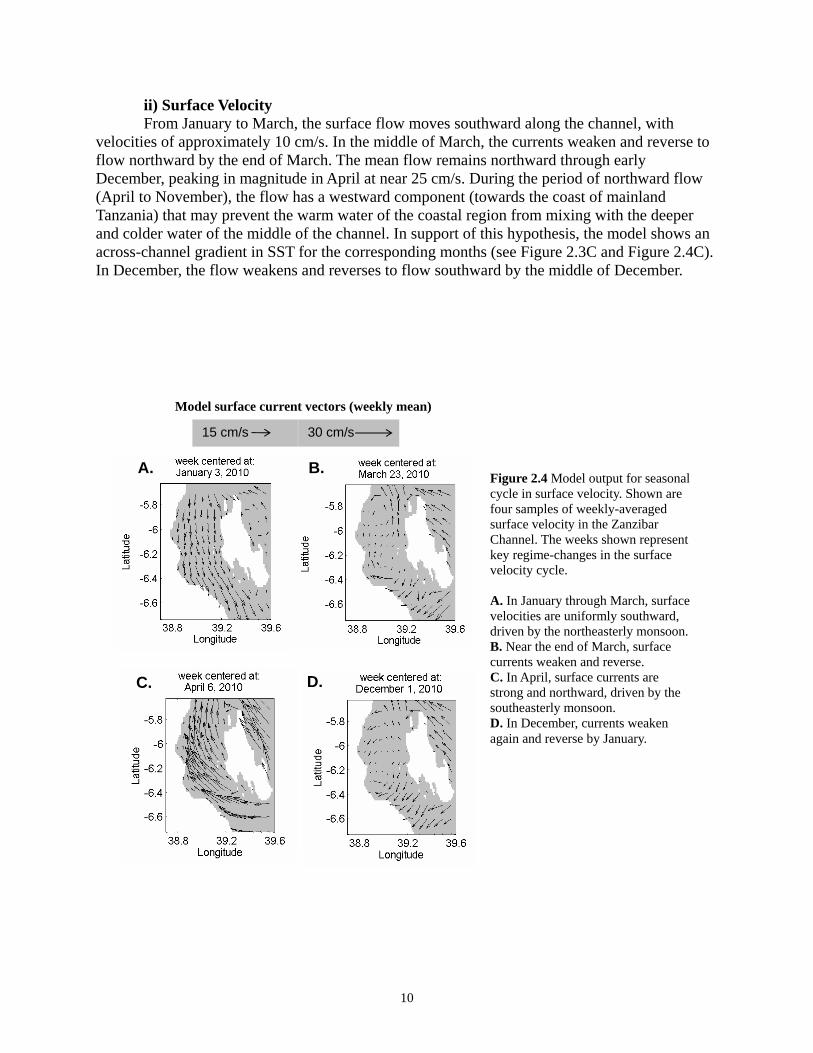
ii) Surface Velocity From January to March, the surface flow moves southward along the channel, with

velocities of approximately 10 cm/s. In the middle of March, the currents weaken and reverse to flow northward by the end of March. The mean flow remains northward through early December, peaking in magnitude in April at near 25 cm/s. During the period of northward flow (April to November), the flow has a westward component (towards the coast of mainland Tanzania) that may prevent the warm water of the coastal region from mixing with the deeper and colder water of the middle of the channel. In support of this hypothesis, the model shows an across-channel gradient in SST for the corresponding months (see Figure 2.3C and Figure 2.4C). In December, the flow weakens and reverses to flow southward by the middle of December.

Figure 2.4 Model output for seasonal cycle in surface velocity. Shown are four samples of weekly-averaged surface velocity in the Zanzibar Channel. The weeks shown represent key regime-changes in the surface velocity cycle. A. In January through March, surface velocities are uniformly southward, driven by the northeasterly monsoon. B. Near the end of March, surface currents weaken and reverse. C. In April, surface currents are strong and northward, driven by the southeasterly monsoon. D. In December, currents weaken again and reverse by January.

Model surface current vectors (weekly mean)

15 cm/s 30 cm/s

A. B.

C. D.

10

2.3.2. Tides Although our main focus is to model on a seasonal scale, the Zanzibar Channel is suspected to be tidally dominated (Mayorga-Adame, 2007), and we have much to gain from an analysis of the tidal currents output by our model. Thus far, our project’s observations have captured cross-sections of the channel for several days. Running our model with solely tidal forcing for the specific days when measurements were taken provides us with a preliminary link between our model and our observations. In addition, models of tidal dynamics in the channel are of great interest to several ongoing projects of our collaborators at IMS.

During flood, tidal currents enter through both channel entrances, converge at the middle of the channel, and reverse during ebb to exit again through both channel entrance. The maximum fluctuation of sea surface height (SSH) occurs in the middle of the channel. A zone of minimal tidal currents appears in this area, where the convergence/divergence of the tidal currents during flood/ebb causes a pilling up/flushing of water (Figure 2.5). The exact position of the convergence oscillates, and therefore the velocities in the middle of the channel are highly variable and difficult to predict.

This peculiar tidal circulation has been suggested in previous studies (Shaghude, et al., 2002) and is supported by recent observations of Mr. Mukaka (D. Mukaka, pers. comm.) and our group.

Model tidal velocity velocities (see scaling bars 15 cm/s)

and sea surface height (see colorbars, m)

Figure 2.5. Surface modeled tidal velocities on top of sea surface height in meters, for August, 5th, 2009 at different times of the day. Hour is in local time (GMT +3 hrs), and the color scale for each frame is different in order to highlight the gradients. Warm colors indicate negative SSH and old colors positive SSH. c

A. Minimal velocities are observed during the transition from flood to ebb. B. During ebb the currents diverge at the middle of the channel. C. In the transition from ebb to flood tide currents reverse. D. During flood currents converge in the middle of the channel.

15:00 hrs

15 cm/s

03:00 hrs

15 cm/s

09:00 hrs

15 cm/s

11:00 hrs

A.

C.

B.

D.

Figure 2.5. Surface modeled tidal velocities on top of sea surface height in meters, for August, 5th, 2009 at different times of the day. Hour is in local time (GMT +3 hrs), and the color scale for each frame is different in order to highlight the gradients. Warm colors indicate negative SSH and cold colors positive SSH. A. Minimal velocities are observed during the transition from flood to ebb. B. During ebb the currents diverge at the middle of the channel. C. In the transition from ebb to flood tide currents reverse. D. During flood currents converge in the middle of the channel.

11

3. Observational Campaign 3.1. Introduction The observational component of the project aims to establish a data set with which to test and improve the ROMS model. In the first year, the goal was to gain preliminary observations with which to evaluate the model results, and to develop a solid technical and interpersonal foundation for the following years.

To set a baseline for channel conditions, the observational team set out to achieve across-channel transects of vertical profiles of temperature, salinity, water velocity and bathymetry. We worked on a traditional sailing vessel (called a dhow) owned by a tour company, temporarily adapting the ship for use as a research vessel. Results from these transects will establish the first comparison of the model results and forcing inputs to real conditions.

In addition, the team deployed three temperature loggers that will provide the project’s future students and collaborators with a yearlong time series of temperature at a key sight at the north end of the channel. Long time series such as this will be essential in validating the seasonality of the model. 3.2. Setup The priority upon arrival to Zanzibar was to procure and equip a boat able to realize cross-channel transects. A local tour boat – fondly dubbed the “research dhow” – was found from a local provider demonstrating a cost-effective sampling method that is reproducible using local resources.

The instruments used during the transects included a Workhorse Sentinel ADCP, lent to the project by Clint Winant at Scripps Institution of Oceanography (SIO), equipped with ‘Bottom Tracking’ and a temperature sensor. When combined with GPS locations, the ‘Bottom Tracking’ feature allows the ADCP, which produces a vertical profile of water velocities at one horizontal location, to provide vertical profiles in a moving boat. In this way, we were able to obtain a snapshot of the water currents along the path of the boat, while recording the bathymetry and the surface temperature. The quality of boat-mounted ADCP data is highly dependent on limiting vibrations in the mounting system. Therefore, a solid and well-regarded handmade mount, a so-called “Kentucky mount”10 was built in San Diego by Robert Thombley, a research technician from SIO. The mount includes a wooden plank attached to the boat to which we attached a metallic pole with the ADCP to be submerged in the water (Figure 3.1).

At designated stations along each transect, we deployed a Seabird SBE-19 CTD profiler, which measures temperature, salinity and in our particular setting fluorescence while lowered down in the water. The instrument and the flourometer were provided by Ralf Goericke and Matt Moldovan, respectively, both at SIO for the duration of the study. A pulley system was developed on the boat to facilitate the process of casting the CTD and obtain smooth profiles (Figure 3.1). To capture across-channel variations in ocean conditions, CTD profiles were measured at designated stations along our cross-channel transects.

At the sites of the CTD casts, biological and water samples were taken for collaborative work with IMS researchers. Water samples were obtained using Niskin bottles at three and seven meters depth, and, immediately after collection, these samples were analyzed for chlorophyll content, oxygen level, temperature, and pH. A net was used to filter the water column for zooplankton samples that will be analyzed later by IMS researchers (Figure 3.2) 10 Reference: http://hydroacoustics.usgs.gov/movingboat/pdfs/KYMount.pdf

12

Figure 3.1 Left panel: Setting the Workhorse Sentinel ADCP and its mount on the research boat. Right panel: Retrieving the SBE-19 CTD from the water after a cast during a transect.

Additional equipment included a GPS to navigate, a portable computer to acquire the

ADCP and GPS data in real time, and a Garmin GPSMAP 420s fish finder to be able to read depth continuously while the ADCP was turned off. The laptop and the fisher finder required a continuous power supply provided by a car battery on board.

Figure 3.2. Left panel: Obtaining subsurface water from a Niskin bottle at a station. Right panel: Retrieving the zooplankton net after a cast during a transect.

Furthermore, to provide the project’s future students and collaborators with seasonal data with which to test the model, three HOBO Temperature Logger where deployed off Tumbatu

13

Island in the northern entrance of the channel. The study site was chosen based on our model results and anecdotal suggestions that there may be a cold intrusion in the north entrance of the channel in January. The loggers will record the water temperature every 2.5 hours for a year at three different depths. The obtained data would help validate the seasonality of the model simulation. The deployment of these instruments is done in close collaboration with Dr. Christopher Musaka from IMS who will maintain and back up the data during the year, and the same time extend the data base time series available in the institute. 3.3. Observational Campaigns A total of three crossing transects were completed. The first two, in July, began in Stone Town in Zanzibar and headed westward until reaching mainland Tanzania. Concurrent work on the model suggested that our planned transect would coincide with the region of convergence and divergence of tidal currents, resulting in poor predictability and large variability of current direction within the area. Therefore, following model results and past publications (Shaghude et al., 2002; D. Mukaka, pers. comm.), we planned our third transect to depart from Stone Town and travel northwest toward regions where tidal currents are more dominant and demonstrate a consistent spatial pattern. The resulting transect was timed to capture the southward currents during flood and northward currents during ebb. The transect path along with the measured bathymetry is shown in Figure 5.3.

Figure 3.3. Trajectories of the three crossing transect. Transects 1 and 2, in the central section of the channel were done in July and the third transect, in a northern section, was realized on August. The black diamonds indicate the stations for CTD and biosampling castings.

14

3.4. Observational Results The dataset resulting from the three transects includes vertical profiles of the water

velocity and surface temperature measurements from the ADCP, temperature and salinity profiles from the CTD, and bathymetry data from both the fish finder and ADCP. The ADCP measurements include three days of data over two separate paths, with a vertical resolution of 2 meters, and a horizontal resolution of about 40m. Figure 3.4 shows a vertical profile of water velocity for the mainland bound of the third transect, in north-south and east-west direction. The bathymetry measured by the ADCP is also shown. In this figure, the phase of the tidal current is evident. Close to the mainland, we observed southward currents corresponding to the flood tide and, in the eastern part of the channel, we observed northward currents corresponding to the ebb phase.

Figure 3.4. Vertical profiles of water velocity from the ADCP during the mainland bound section of the transect realized on August 05. The upper panel shows the north-south component of the velocity (m/s) and the lower panel the east-west component. Around 39 degrees of longitude the change of phase of the tide occurred, from ebb to flood.

The north-south currents show a mostly uniform vertical section and abrupt direction change between tide phases. Therefore, we calculate the mean current averaging the velocities along the vertical. Figure 3.5 shows the mean current for the three crossing transects. The upper panels show both July transects, both during an ebb phase of the tide. The inconsistency in the direction of the flow indicates the particular area of the channel where waters converge and diverge with the tides. We chose to direct the third transect more northward (see lower panel in Figure 3.5), hypothesizing that we would observe a southward current (a flow toward mid-channel) during the flood phase and a northern current (a flow exiting the channel) during the ebb phase.

15

Figure 3.5. Mean velocity of the water column for all the crossing transects. Upper panel: Mean current for July 15 and July 24, ebb phase of the tides. Lower panel: Mean current for August 05, left panel channel mainland bound, right panel Zanzibar bound. The CTD castings produced twenty-three vertical profiles of temperature and salinity at

evenly spaced stations along the transect paths (see Figure 3.3) for different times of the day. Figure 3.6 exemplifies the temperature profiles at stations along the second transect line (see Figure 3.3 for the location of the transect line). The temperature is slightly stratified in the middle of the channel due to solar heating, but is otherwise well mixed; the change in temperature in the vertical is around 0.5°C. In the stations closest to Stone Town, temperature was more uniform in the vertical, perhaps due to mixing produced by notably strong wind forcing at the time we passed and by turbulence due to rough bathymetry.

The closest station to mainland shows a larger difference in temperature, observed also in the salinity profile and in the northern transect, suggesting that the shallow coastal shelf on the mainland side isolates the water residing there. This difference in the water properties was also observed in oxygen content and pH.

16

Figure 3.6. Temperature vertical profiles for the CTD casts realized during the crossing transect on July 24. Note that we station cast was done during a different time of day and different atmospheric and ocean conditions.

17

4. Comparison of Model to Observations 4.1. Temperature

The model reproduces the qualitative features of the seasonal cycle as reported previously (Harvey 1977; Mohammed et al. 1993; Shaghude et al. 2002). We compared monthly-averaged in-channel sea surface temperature from model to those of the CoRTAD. CoRTAD contains weekly global sea surface temperature (SST) from 1985 through 2005, with a spatial resolution near 4 km. For averaging, the channel mouths were defined by the 200 km isobath, and grid cells shallower than 15 m depth were excluded (Figure 3.3). For ten months of the year, monthly mean sea surface temperatures the ROMS model output agreed with those of CoRTAD to within two standard deviations (Figure 4.1). In March and December, the ROMS model SST exceeded CoRTAD SSTs, likely due to previously-identified problems with the implementation of heat fluxes in the model. Although it is evident that the model overestimates SST during the months of March and December, the model reproduces observed qualitative seasonal patterns. A revised version of the model will provide more accurate results (see Section 6, Future Work).

Figure 4.1. Comparison of CoRTAD and ROMS monthly mean sea surface temperature in the Zanzibar Channel. Errorbars show plus and minus one standard deviation in CoRTAD SST for 1985-2005. For averaging, the Zanzibar Channel is defined by the 200-m isobaths at the N and S entrances, and SST values in shallow regions (less than 15-m depth) are excluded.

18

Figure 4.2. Observed and simulated temperature profiles for the crossing transect realized on August 05, along with the measured bathymetry from the FishFinder and the “simplified” bathymetry used in the model.

The temperature profiles observed during our campaigns are similar to those produced by the model (see Figure 4.2), both in mean values and in vertical and horizontal distribution. Slight stratification was predicted, as were warmer temperatures in the shoal on the western boundary of the channel. The observed bathymetry differs from the smoothed bathymetry used in the model. In the future, the model will be changed to capture the mixing produced by rough bathymetry, and may incorporate more accurate bathymetry obtained from the ADCP and the FishFinder during the campaigns. 4.2. Salinity

The model salinity profiles are different from observations in the mean value and in horizontal gradient (Figure 4.3). Model salinity and temperature are highly correlated, while observed salinity shows little relation to observed temperature. It is possible that the system is driven by some other important forcing absent in the model. Local inputs like rivers or waste dumping near Stone Town may be important in the Zanzibar Channel system, and should be investigated in future observational and modeling work.

19

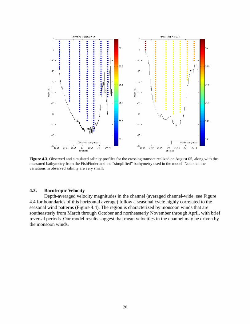
Figure 4.3. Observed and simulated salinity profiles for the crossing transect realized on August 05, along with the measured bathymetry from the FishFinder and the “simplified” bathymetry used in the model. Note that the variations in observed salinity are very small. 4.3. Barotropic Velocity

Depth-averaged velocity magnitudes in the channel (averaged channel-wide; see Figure 4.4 for boundaries of this horizontal average) follow a seasonal cycle highly correlated to the seasonal wind patterns (Figure 4.4). The region is characterized by monsoon winds that are southeasterly from March through October and northeasterly November through April, with brief reversal periods. Our model results suggest that mean velocities in the channel may be driven by the monsoon winds.

20

4.4. Tidal Velocities

Tidal currents in the Zanzibar Channel enter and exit through both the north and south entrances, converging during the flood and diverging during the ebb in the mid-channel, off Stone Town (Shaghude et al., 2002). Given the magnitude and frequency of the tidal current in comparison with the net flow, during our three crossing transects we are only measuring the tidal current.

The model running only with the tidal forcing compares well with both our observations for one day (see Figure 4.5 and 4.6), and with previous results (Shaghude et al., 2002) for the convergence-divergence cycle during the flood and ebb. Although magnitude of currents are not equal for both sets, the model and observations show the same pattern of changes in magnitude and direction during the different phases of the cycle.

When the model is run with all available forcing – atmospheric, tidal, and that of global model temperatures and velocities – the current velocities do not coincide with the observations in either magnitude or direction (not shown). This suggests that other factors such as day-to-day atmospheric variability and interannual variability in the EACC might also play an important role.

W E

N S

scale (cm/s)

current 30 20 10

0

Monthly mean vectors wind

300 200 100

0

Figure 4.4 Comparison of monthly mean observed winds and model current velocities in the channel. Current velocity, shown in black, is averaged in time (monthly), vertically (depth-averaged), and horizontally (in the channel – see Figure 3). Wind velocity is from a metrological station in Stone Town (see Figure 1.1), averaged monthly. The averaged currents follow the monsoon wind pattern.

21

Figure 4.5 Mean current during the crossing transect on August 5 showing the tidal currents. The eastern section

f

occurs during the ebb, and the western section (both mainland bound and Zanzibar bound) show the flood phase othe tide.

Figure 4.6 Comparison of the observed and modeled north-south velocity component at different depths. The color scale shows the magnitude in m/s.

22

5. Collaborations and Ongoing Projects 5.1 Contacts with the IOC and the oceanographic community in the East African region 5.1.1 Visit to Kenya by Jurgen Theiss

Jurgen Theiss made a trip from Zanzibar to Kenya to obtain a better overview of coastal oceanography in East Africa as part of an ongoing effort to integrate more effectively the Zanzibar Project into the activities in the region and to discuss opportunities for possible future collaborations. Stefano Mazzilli at the Nairobi Office of the Intergovernmental Oceanographic Commission (IOC) helped organize this trip and also hosted Jurgen Theiss while he was visiting Nairobi.

Jurgen Theiss visited the Kenya Marine Fisheries Research Institute (KMFRI) in Mombasa and together with Stefano Mazzilli the Kenya Meteorological Department (KMD) in Nairobi. At both institutions he met with the respective Deputy Director and mainly with the research groups working on coastal modeling. It was determined that the modeling objectives at the Kenyan institutions are similar to those at IMS and thus also to those of the Zanzibar Project. It was agreed that it would therefore be of mutual benefit to communicate more closely in the future about the various modeling efforts. KMFRI suggested that the tour boat that we converted into a research vessel (“research dhow”) could next year also cruise from Zanzibar through the Pemba Channel and onto Southern Kenya to make measurements that would be of great interest to both countries. KMFRI indicated that they would in principle be able and interested in funding such a cruise. At KMD it was also discussed how the buoy array that the international community is currently installing in the Indian Ocean could be used for coastal modeling in East Africa. Furthermore, KMD, as the operator of the regional weather forecasting, offered to make wind fields of interest to our model available to us. In general, both KMFRI and KMD would like to stay in close contact with the Zanzibar Project as this would be of benefit to the entire region and the foundation for possible future collaborations. 5.1.2 Visit by Stefano Mazzilli of the Intergovernmental Oceanographic Commission

Stefano Mazzilli visited Zanzibar for about a week at the end of July. He was interested in meeting the other members of our team and learning about our project’s methods and results. We discussed the potential uses of our work for other collaborative projects. From this experience, a better interpersonal relation was created with IMS researchers and new collaborative projects began to develop with both IMS and the Tanzania Fisheries Research Institute (TAFIRI).

We also accompanied Mr. Mazzilli to Paje, in the eastern part of Zanzibar, to meet with a NGO dedicated to conservation. The objective was to connect the NGO to IMS researchers in order to promote collaborative solutions to their shared conservation goals. 5.2 Deployments of the project’s fish finder for collection of bathymetry data. Of particular interest to the local oceanographic community was the capability of the project’s fish finder unit to collect extensive bathymetry data. The fish finder combines a GPS unit, an echo sounding device, and an internal memory and achieves completely automated recording of bathymetric data. This capability simplifies the process of bathymetry data collection used in existing projects, and allowed for collection of bathymetry data on cruises which otherwise would not have done so.

Under the supervision of Dr. Shigalla Mahongo the project’s fish finder was deployed on

23

a 12-day TAFIRI stock assessment cruise. This collaborative effort paid off yielding valuable athymetry data for Dr. Mahongo’s current modeling effort which focuses on the broader coastal

In addition, Ignantio Sanga, an IMS researcher studying coastal erosion on the eastern der to take more extensive bathymetry data in his

study a

t

5.3

n

4 Conference of the African egional Group of the International Association of Aquatic and Marine Science Libraries and

resourc

ts to

attend a

Andy Hooten, Executive Secretary of the World Bank’s Targeted Research and Capacity our work

bregion of Tanzania and is funded by a START International grant.

coast of Zanzibar, used the project’s fish finrea. His work is part of the Regional Coastal Management Program of the Indian Ocean

Countries (known as ReCoMaP), a project supported by the IOC. Owing to the success of these efforts and support from Stefano Mazzilli from the IOC,

we prepared a report on the specifics of data collection using the fish finder. We hope this reporwill prove useful to other interested oceanographic institutions in the region.

Collaborative work with IMS and TAFIRI

Dr. Shigalla Mahongo, from TAFIRI, is now one of the key contacts in Tanzania for the Zanzibar Project’s efforts and recently spent several weeks in Zanzibar working in conjunctiowith the project in the modeling part. Clement Majuto, from IMS, worked in collaboration with the modeling group to develop a model of the Pemba Channel, his area of study. He is currently developing a proposal for START International that would allow him to develop and validate a model of the Pemba Channel in a similar project as ours.

Dr. Aviti Mmochi and Dr. Musa Chacha, both from IMS, work on ocean chemistry and participate, directly and indirectly, in our cruises to obtain oxygen and pH content measurements in the Zanzibar Channel. Dr. Christopher Muhando of IMS, is one of our key collaborations at IMS as we united efforts for the deployment of temperature loggers in the north part of the Channel. 5.5 AFRIAMSLIC Conference

Marisol Garcia-Reyes and Patrick Nadeau attended the th

RInformation Centers for one day. They attended lectures addressing the issue of sharing data

es in the African scientific community. 5.6 IMS Seminar in preparation for WIOMSA 2009

Before attending the WIOMSA meeting in Reunion Island, IMS researchers and studenpresent their work for their colleagues in order to prepare for the meeting. We were invited

nd took the opportunity to learn in more detail the research realized at IMS. 5.7 CRTR Executive Secretary

Development for Management (CRTR) program visited IMS. He was very interested inand saw a potential use of our results in their own work. He offered us to find out whether we can use their current meters. He advised Gabriela on her PhD proposal.

24

6. Future Work 6.1 Modeling

Future modeling efforts will integrate observed bathymetry and will continue to compamodel outputs to observed currents, temperatures, and salinity. In this year of the study, poweroutages led model runs to be interrupted several times and, unfortunately, restarting the model can introduce errors. In future years of the project, students will try

re

to run the model without interrup

dress transport of sedime

achieved by mooring the ADCP several days or more so

least deploy

arious depths and at various horizontal positions in the channe

le in validating the magnitude and timing of the tidal currents of the odel.

the northern nd southern entrances of the channel will be of most value.

tions. In addition, future students may run the model with improved heat fluxes and surface forcing and may include freshwater discharges to improve the modeled salinity. The project hopes to expand the model to include other modules of ROMS that ad

nt, biota, and pollutants.

6.2 Observations In order to capture mean, seasonal-scale flow through the channel, longer time series of

current data are required. This could bethe tidal currents can be filtered out to isolate mean flows.

To observe the channel’s seasonal cycle, the project must seek measurements with atmonthly time-resolution for several years. We suggest working with researchers at IMS to and maintain temperature loggers at v

l. Sampling cross-sections of currents, temperature and salinity profiles, as we did this year,

will continue to be valuabm Additional transects also will add to the growing set of bathymetry data in the channel. Our transects were restricted to the central region of the channel, and future work ina

25

7. Acknowledgements

to thank Jurgen Theiss for all of his time, effort, and enthusiasm in develop

ll

e

hristopher Muhando, and Daudi Mukaka. e also want to thank the boat owner Khamis Khamis for allowing us to convert his tour

. Our work on the boat would have been impossible without the help of Juma M

ile n Zanzibar. Many others have contributed prior to our time in Zanzibar and will

continu

We would like ing and coordinating the project. We would also like to thank Javier Zavala-Garay for

supervising the ROMS modeling work, and Robert Thombley for providing technical assistancein the observational work.

IMS has been a welcoming and supportive host. We are grateful to its management, inparticular to Margaret Kyewalyanga, Ntahondi Nyandwi, and Edna Nyika, for attending to aadministrative issues that our visit entailed and thus allowing us to focus fully on our work. Walso enjoyed the general support and scientific discussions with many IMS researchers, especially Yohanna Shaghude, C

Wboat into a research vessel

akame, for which we are thankful. We enjoyed the productive visits of Shigalla Mahongo from Dar es Salaam and of

Stefano Mazzilli from Nairobi. We are grateful that Clint Winant, Ralf Goericke, and Matt Moldovan lent has at no cost

to our project their ADCP, CTD, and flourometer, respectively. These acknowledgements mainly mention only those that contributed to the project wh

we were ie to contribute in the future. They are mentioned on the Zanzibar Project’s web site. Funding for this project has been provided by the National Science Foundation (OISE-

0827059) and The Meinig Family Cornell National Scholars.

26

References Haidvo and

Harvey3,

ocean with error

tion of the Zanzibar Channel: A Modeling Approach.”

nation of the effects of pollution

ine

uzaki, J. Woollen, S-K Yang, J.J.

nilo, M. Fiorino, and G. L. Potter. 1631-1643, Nov 2002, Bul. of the Atmos. Met. Soc. ttp://www.cpc.ncep.noaa.gov/products/wesley/reanalysis2/kana/reanl2-1.htm

ewell, B.: 1957, A preliminary survey of the hydrography of the British East Africa Coastal waters. Colonial Office Fishery Publication 9, HMSO, London.

gusaru, A. and S. Mohammed: 2002, “Water, salt and stoichiometrically linked nutrient budgets for Chwaka Bay, Tanzania.” Western Indian Ocean J. Mar. Sci., 1, 97:106.

Shaghude, Y., K. Wannäs, and S. Mahongo: 2002, “Biogenic assemblage and hydrodynamic

settings of the tidally dominated reef platform sediments of the Zanzibar Channel.” Western Indian Ocean, J. Mar. Sci., 1, 107-116.

Shchepetkin, A. and J. McWilliams: 2005, “The Regional Ocean Modeling System: A split-

explicit, free-surface, topography following coordinates ocean model.” Ocean Modeling, 9, 347-404.

Swallow, J.: 1991, Structure and transport of the East African Coastal Current. J. Geophys. Res.,

96, 22, 245-222, 257.

gel, et al.:2008, “Ocean Forecasting in Terrain-Following Coordinates: FormulationSkill Assessment of the Regional Ocean Modeling System.” Journal of Computational Physics 227, 3595-3624

, J.: 1977, “Some aspects of the hydrography of the water off the coast of Tanzania: A contribution to CINCWIO.” University Science Journal - University of Dar es Salaam, 53-92.

Hellerman, S. and M. Rosenstein: 1983, Normal wind stress over the world

estimates. J. Phys. Ocean., 13, 1093-1104. Mayorga-Adame, G.: 2007. “Ocean Circula

http://www.zanzibarproject.org/students/mayorga-adame/mayorga-adame_final_report.pdf

Mohammed, S., A. Ngusaru, and O. Mwaipopo: 1993, “Determion coral reefs around Zanzibar Town: A technical report to the National Environment Management Council, Dar es Salaam, Tanzania.” Technical report, Institute of MarSciences, Zanzibar, University of Dar es Salaam.

NCEP-DEO AMIP-II Reanalysis (R-2): M. Kanamitsu, W. EbisHh

N

N

27