Modeling of the Microbial Quality of Food
158
Modeling of the Microbial Quality of Food 'ÖÖÖ0 0545
Transcript of Modeling of the Microbial Quality of Food

Modeling of the Microbial Quality of Food
'ÖÖÖ0 0545

WAOLNÜNGEM
Promotoren: dr. ir. K. van 't Riet
hoogleraar in de levensmiddelenproceskunde
dr. ir. F.M. Rombouts
hoogleraar in de levensmiddelenhygiëne en -microbiologie

Marcel Zwietering
Modeling of the Microbial Quality of Food
Ü » sB3
Proefschrift
ter verkrijging van de graad van doctor
in de landbouw- en milieuwetenschappen
op gezag van de rector magnificus,
dr. C.M. Karssen,
in het openbaar te verdedigen
op woensdag 29 september 1993
des namiddags te vier uur in de Aula
van de Landbouwuniversiteit te Wageningen
,. ;

ABSTRACT
Zwietering, M.H. (1993) Modeling of the Microbial Quality of Food. Ph.D. thesis,
Agricultural University Wageningen (152 pp., English and Dutch summaries)
Keywords: Modeling, microbial growth, temperature, growth curves, model validation,
temperature shifts, decision support systems (DSS).
In this thesis it is shown that predictive modeling is a promising tool in food research,
to be used to optimize food chains. Various models are developed and validated to be used to
describe microbial growth in foods.
A tool is developed to discriminate between different models and to restrict the number
of parameters in models. Models to describe a growth curve and to describe the effect of
temperature, and the effect of shifts in temperatures, are developed and validated with a large
amount of experimental data.
Furthermore, a procedure is developed to couple quantitative and qualitative
information in a structured manner. Simple procedures to make (preliminary) shelf-life
predictions are given, as are procedures to extend these (simple) models.
The most important advantage of modeling is that insight is gained in the progression
of microbial growth within a product chain. Furthermore, these models are shown to be
essential to calculate quality changes with the use of decision support systems (DSS).

CIP-GEGEVENS KONINKLIJKE BIBLIOTHEEK, DEN HAAG
Zwietering, Marcel
Modeling of the microbial quality of food / Marcel
Zwietering. - [S.l. : s.n.] - 111.
Thesis Wageningen. - With ref. - With summary in Dutch.
ISBN 90-5485-143-0
Subject headings: microbiology of food.

STELLINGEN
1. Smith (1985) doet ten onrechte uitspraken over temperatuurdentlijnen in slachthuizen,
omdat hij warmte-indringing in het vlees niet in beschouwing neemt.
Smith M.G. (1985). The generation time, lag time, and minimum temperature of growth of coliform
organisms on meat, and the implications for codes of practice in abattoirs. J. Hyg. Camb. 94: 289-300.
2. Barreto et al. (1991) verklaren hun resultaten met een 'apparent lag time', veroorzaakt
door een levensvatbaarheid lager dan 100%. Dezelfde resultaten kunnen ook verklaard
worden met een normale lag-fase en 100% levensvatbaarheid.
Barreto M.T.O., E.P. Melo, J.S. Almeida, A.M.R.B. Xavier, and MJ .T . Carrondo (1991). A kinetic
method for calculating the viability of lactic starter cultures. Appl. Microbiol. Biotechnol. 34:648-652.
3. De modellen gepresenteerd door Beal en Corrieu (1991) voorspellen onder andere een
rechtlijnig verband tussen pH en de maximale specifieke groeisnelheid van
Lactobacillus bulgaricus. Het desalniettemin vermelden van een optimale pH voor deze
groeisnelheid wijst erop dat de auteurs een computerprogramma gebruiken dat
extrapolaties niet toestaat.
Beal C , and G. Corrieu (1991). Influence of pH, temperature, and inoculum composition on mixed
cultures of Streptococcus thermophilics 404 and Lactobacillus bulgaricus 398. Biotechnol. Bioeng.
38:90-98.
4. Het gebruik van vijfendertig parameters om het effect van vier variabelen te beschrijven
in een derde-ordepolynoom resulteert niet in een vergroot inzicht en kan bovendien in
gevaarlijke voorspellingen resulteren.
Palumbo S.A., A.C. Williams, R.L. Buchanan, and J.G. Phillips (1991). Model for the aerobic growth
of Aeromonas hydrophila K144. J. Food Protection 54:429-435.
5. Een neuraal netwerk is vaak een eufemisme voor fitten met teveel parameters.
bijvoorbeeld: LinkoP., K. Uemura, Y.H. Zhu, andT. Eerikäinen (1992). Application of neural network
models in fuzzy extrusion control. Food and Bioproducts Processing 70:131-137
6. Modellering is essentieel voor het gestructureerd verzamelen van voldoende gegevens.
7. De krant is een van de meest bederfelijke produkten.

8. Combinatie van Just In Time (JIT) met Murphy's Law resulteert in Just Too Late (JTL)
en ontevreden klanten.
9. Bij het berekenen van kengetallen voor kwaliteit van onderzoek door auteurschappen
van wetenschappelijke publikaties op te tellen, wordt vaak vergeten te delen door het
aantal auteurs.
10. Bij het gebruik van het begrip % dient de noemer duidelijk gedefinieerd te zijn.
11. Door het gebruik van spellingscontroleprogrammatuur worden steeds meer woorden,
die in het Nederlands aan elkaar geschreven moeten worden, niet meer aan elkaar
geschreven.
12. Drieduizend j aar voor onze j aartelling ondervonden de oude Egyptenaren dat een zuiver
beeldschrift tekort schiet om alles op te tekenen. Nu, 5000 jaar later, blijkt opnieuw dat
pictogrammen minder begrijpelijk zijn dan hun ontwerpers zich voorstelden.
K. Th. Zauzich (1980). Hieroglyphen ohne Geheimnis. P. von Zabern, Mainz am Rhein.
Microsoft Windows version 3.1® 1985-1992 Microsoft Corp.
13. Als een regering haar volk probeert te overtuigen van de veiligheid van kernenergie
dient zij de toekomstige centrales in de buurt van de regeringsgebouwen te plannen.
14. Het aan de buitenkant aanbranden van vlees bij het barbecuen heeft als voordeel dat de
(actieve) kool al gelijk met de, aan de binnenkant overlevende pathogenen,
geconsumeerd wordt.
Stellingen behorende bij het proefschrift "Modeling of the Microbial Quality of Food"
M.H. Zwietering
Wageningen, 29 September 1993

CONTENTS
Chapter 1
Introduction: Modeling microbial quality of food 1
Chapter 2
Modeling of the bacterial growth curve 9
Chapter 3
Comparison of definitions of the lag phase and the exponential 27
phase in bacterial growth
Chapter 4
Modeling of bacterial growth as a function of temperature 41
Chapter 5
Evaluation of data transformations and validation of models for 65
the effect of temperature on bacterial growth
Chapter 6
Modeling of bacterial growth with shifts in temperature 87
Chapter 7
A decision support system for prediction of the microbial spoilage in foods 111
Chapter 8
Concluding remarks: Extended use of predictive modeling 127
Summary 147
Samenvatting 149
Nawoord 151
Curriculum vitae 152

CHAPTER 1
INTRODUCTION:
MODELING MICROBIAL QUALITY OF FOOD
FOOD QUALITY
Definition. Food quality can be defined as the sum of the characteristics of a food that
determine the satisfaction of the consumer and compliance to legal standards. Thus, food
quality is a combination of numerous factors, such as organoleptic properties (e.g., texture,
taste, flavour, smell, colour), nutritional value (e.g., caloric content, fatty acid composition),
shelf life (e.g., microbial number), and safety conditions (e.g., presence of pathogens, toxins,
hormones). Some of these (e.g., microbial numbers) can be relatively easily quantified, while
others are very difficult to assess (e.g., taste). Food quality thus cannot be quantified in every
detail, and overall quantification depends strongly on the priority among quality determining
aspects. To determine total food quality, quality indicators are needed and must be weighted,
since their relative importance depends on product, trends, producer, and market.
Significance. Food quality attracts ever more attention and prediction of the rate of
quality loss is important for the following reasons:
The food market is subject to saturation in most cases, therefore, quality becomes more
important than quantity.
There are new quality attributes which are highly appreciated by the modern consumer
(in contrast to traditional quality demands). Consumers show an increasing interest in
convenience foods with the appearance and taste of fresh products and in food quality
Part of this chapter was used for the publication:
Some Aspects of Modelling Microbial Quality of Food
M.H. Zwietering, F.M. Rombouts, K. van 't Riet (1993)
Food Control 4:89-96

INTRODUCTION
aspects such as flavour and (assumed) health aspects (e.g., nutritional value, fatty acid
quantity and composition, energy content, salt concentration, presence of additives such
as preservatives).
Consumers are willing to pay a higher price for quality.
Manufacturers want to deliver constant quality products at the lowest costs.
Many products have a limited shelf life. Production and storage conditions affect quality
very strongly; therefore, production and distribution are often critical. From the past
there are many dried, salted, frozen, and sterilised products, while nowadays chilled
and intermediate-moisture foods are becoming more important.
The shelf life of a product determines the distribution regime: daily delivery for
perishable products such as fresh milk, bread, fresh vegetables, and fresh meat, or less
frequently as for salads, margarine, etc.
Due to more open borders in the European Community (EC), the distribution routes
have become longer, and therefore, there is a need for an increased shelf life.
In some areas there is a rather rapid product development (changes in product
formulation). Consequently, it will be useful to make an estimation of the shelf life
during product development.
Formulation of products may be different in different countries or regions, because of
legal requirements or regional food preferences. Therefore, it would be useful to know
the effect of different compositions on the shelf life, to avoid each formulation requiring
a laborious shelf-life test.
New procedures are being developed to meet these quality demands, such as new
technologies (e.g., microwave heating, ultrahigh temperature (UHT) processes, modified
atmosphere packaging, supercooling, irradiation), and new strategies (e.g., logistics and
modeling).
Quality loss along a chain. Quality loss can result from microbial, chemical,
enzymatic, or physical reactions. Various factors influence quality loss, such as the
composition of the product. A product without lipids, for example, cannot show lipid
oxidation; iron (Fe3+) acts as catalysing agent for vitamin C degradation (2). Other factors
influencing quality loss are processing and storage conditions (temperature, time, packaging
material, gas atmosphere, machinery).

CHAPTER 1
Thus, product quality is determined by the composition and quality of the raw materials,
and by the process and storage conditions. Quality is often measured during production and
distribution by taking samples of a product somewhere along the chain (Fig. 1). This can give
valuable information about long-term quality changes and bottlenecks in the line. This,
however, gives little information about the separate effect of particular process steps in the
production and distribution chain on the total quality. It is important to get insight in the
progression of the deterioration reactions, '\.f. the kinetics of spoilage in each step in the
process. Quality loss can be determined by a single processing step, but can also result from
partial losses at several stages of the production or distribution. Without insight it is
impossible to optimize the process, and to evaluate changes in costs in relation to changes in
quality. It is therefore useful to examine the whole chain of food products from raw materials
to consumption (Fig. 1).
raw materials
production
pasteurisation
storage
distribution
storage
consumption
sample
sample
sample
FIG. 1. Example for a pathway of a food product from raw materials to consumer.
Modeling can be a useful tool to get insights into the importance of factors in any part
of the production and distribution chain, and is based on quantitative predictions of the rate
of spoilage. Such modeling allows prediction of the quality or shelf life of products, detection
of critical points in the production and distribution process, and optimization of production

INTRODUCTION
and distribution chains by combining cost models with the spoilage models. Moreover, by
making the models and by evaluating the predictions, insight in the relevant processes can be
obtained.
PREDICTIVE MODELING
Significance. Predictive modeling is a promising methodology in food research, to be
used to optimize food chains. Models are used to describe deterioration under different
physical or chemical conditions such as temperature (7), pH, and water activity (av). First,
deterioration reactions have to be modeled and the models must be validated with quantitative
data. The model parameters can then be estimated. These models and model parameters will
only be valid for the product and the conditions for which the data are collected. However,
in some cases the model parameters and/or the model will also hold for similar products and
conditions.
In some cases, certain deterioration reactions can be excluded. For example, if the aw
of a product is lower than 0.6, microbial growth can be excluded and if the aw is lower than
0.2, Maillard browning activity can be excluded (2). If the physical and chemical conditions
of the product allow a specific deterioration reaction, an estimate can be made of the kinetics
of the reaction. For example Escherichia coli can grow between pH 4.4 and 9.0 (4). If the
pH of a product is 4.6, Escherichia coli can still grow in that product, but not very fast (and
slower than at pH=5). To predict the kinetics of the various deterioration processes more
quantitatively, models describing the effects of different conditions are essential. Several
models are known to predict deterioration reactions. Examples are given by Ratkowsky et al.
(3) and Zwietering et al. (5) to describe the effect of temperature on microbial growth. For
the effect of pH a parabolic behaviour can be assumed, for instance. The Arrhenius model (1)
can be used for the temperature effect on chemical and physical processes. The resulting
quantitative estimation can be used to predict the shelf life.
For the validation of the models numerous measurements are needed. However, once
the model is validated, predictions can be made with none, or only very few, experiments,
and insight into the process is gained.
It is often useful to search for literature models and literature parameters for comparable
products and microorganisms (Fig. 2). With such models and parameters preliminary
predictions can be made and insight can be gained. This can also be very useful for

CHAPTER 1
experimental design. From the discrepancy between these predictions and actual data,
strategies for improvement may be derived, such as better models and/or better parameter
estimates.
Especially microbial risks have increased due to the trends mentioned before. From the
past there were many dried, salted, frozen, sterilised products. So in the past growth limits
(aw, salt, T) and inactivation kinetics (during sterilization) were of importance. Growth was
not possible, since the organisms were absent (sterilisation) or the conditions were changed
so that growth was not possible (dried, salted, frozen). Nowadays chilled and
intermediate-moisture foods are becoming more important. Then, growth kinetics and the
effect of shelf life increasing factors (e.g., T, aw, pH) on the kinetics are of larger importance.
Moreover, the modern consumer often wants a lower salt concentration, and absence of
additives such as preservatives. This emphasises the need to determine the effect of
combinations of factors that are of importance for the growth of micro-organisms.
literature models
order of magnitude insight
model knowledge statistics ^
experiments
FIG. 2 . Schematic representation of a procedure to make kinetic predictions of food deterioration processes.

INTRODUCTION
Values and needs in predictive modeling. The most important needs in predictive
modeling are:
A good procedure to describe growth curves of microorganisms.
Tools to discriminate between different models.
Models that are validated with a large amount of experimental data.
Models for shifts in variables (these are scarce).
Protocols to extend quantitative models with qualitative knowledge.
Models to describe the effect of additional variables (only a few variables have been
investigated, such as T, a„, pH).
Integrated models for the combined effect of multiple factors, and determination of
interaction terms.
Objectives of modeling. The value of a model is strongly dependent on the objective
for which the model is used. For instance the control of a certain variable (y) by a control
variable (u), (e.g., pH control of a fermentor) often only requires a simple model (on-line
feedback). Only a global description of the dynamic behaviour of y as function of u is
sufficient, to obtain the right value for the control signal. Subsequently, y is measured again
and if the value is not correct the control procedure will continue, resulting finally in the
desired value. On the other hand, if one wants to predict the death rate of Clostridium
botulinum spores in a sterilisation procedure, the global dynamic behaviour will often not be
sufficient, and a much more accurate model is necessary, since there is no feed back (or only
off-line). In other cases, the aim can be to understand more mechanistically what happens
during sterilisation. A more mechanistic model is then necessary, which must be validated
with experimental data. In some cases this model is only used to test a hypothesis and it does
not need to be very accurate in predicting.
Warning note. Modeling techniques can be very useful. However, with models and
also with computer programs nonsense can be generated. It is, therefore, of great importance
that modelers combine knowledge in food science, informatics, and mathematics, and use the
expertise of all these disciplines to detect possible errors. Computer programs and
mathematical equations may yield predictions which deviate enormously from reality.
Therefore, a food scientist must be sceptical about predictions. An example of this can be
shown with the gravity acceleration (g=9.81 m/s2 in The Netherlands) and Newtons laws.
With only the gravity acceleration, the position and velocity of a falling stone and of a falling
ashtray can be predicted. A falling leaf however gives totally different results, since the air

CHAPTER 1
resistance and air flow phenomena are of large influence, so the gravitational acceleration,
the air resistance, and the direction of the air flow are of importance, which makes the
problem more complex. So the acceleration will be equal to the gravity acceleration in some
cases, but will markedly deviate in other cases. Also the model will be valid in certain ranges
only, since Newtons laws are not valid if velocities approach light velocity.
CONCLUSIONS
Modelling can be an important tool to predict the shelf life of products, to optimize
production and distribution chains, and to gain insight about important variables that
determine product deterioration. Predictive models, kinetic data, expertise, logistics, and
simulation and optimization routines can be combined to support decisions in production and
distribution, and product development. This can help to determine possible spoilage
organisms, and changes in growth rates of organisms can be estimated when the physical
properties are changed.
OBJECTIVE OF THIS THESIS
In this work a procedure to compare different models will be examined. With this
procedure a model will be selected to describe a bacterial growth curve and to estimate the
specific growth rate, lag time and asymptote from growth data by examining a large amount
of growth curves. Furthermore, models for the effect of temperature on the growth rate will
be compared, with a large amount of growth rates at different temperatures. Models for the
effect of temperature on the lag time and the asymptote will be selected. Furthermore, the
effects of shifts in temperature will be examined. A larger system to collect modeling results,
parameter values and expertise will be built in order to combine quantitative and qualitative
information. This will be developed as a decision support system.
OUTLINE OF THIS THESIS
In Chapter 2 of this thesis a comparison is made between different models that describe
bacterial numbers as a function of time. The models are reparameterized so that they contain
biologically meaningful parameters. A procedure to estimate growth parameters from a set of
data is given. In Chapter 3 the method as described in Chapter 2 is compared with other
methods, as described in literature. In Chapter 4 different growth/temperature models are

INTRODUCTION
compared. In Chapter 5 the correct variance-stabilising transformations are determined with
a large amount of data and the models of Chapter 4 are validated and updated. In Chapter 6
the effect of temperature steps on bacterial growth is evaluated. In Chapter 7 the first steps
are taken to build a knowledge-based system, which can help to detect possible spoilage
organisms and which can estimate growth parameters. In Chapter 8 (general discussion) the
models are discussed and some examples are given. Possibilities to combine the models with
models for heat transfer and logistics are given. These combined models can be used in
simulation programs, that predict the outgrowth of bacteria as function of time and location
inside the product, in food chains, with different storage temperatures. The result of this work
is evaluated, and future expansions are proposed.
REFERENCES
1. Arrhenius, S. 1889. Über die Reaktionsgeschwindigkeit bei der Inversion von Rohrzucker durch Säuren. Z. Phys. Chem. 4:226-248.
2. Fennema, O.R. 1985. p. 56,57,489. In Food Chemistry. Marcel Dekker, New York. 3. Ratkowsky, D.A., R.K. Lowry , T.A. McMeekin, A.N. Stokes, and R.E. Chandler. 1983.
Model for bacterial culture growth rate throughout the entire biokinetic temperature range. J. Bacteriol. 154:1222-1226.
4. Silliker, J.H., R.P. Elliot, A.C. Baird-Parker, F.L. Bryan, J.H.B. Christian, D.S. Clark, J.C. Olson, and T.A. Roberts. 1980. p. 101. In Microbial Ecology of foods. Volume 1. Academic Press, New York.
5. Zwietering, M.H., J.T. de Koos, B.E. Hasenack, J.C. de Wit, and K. van 't Riet. 1991. Modeling of bacterial growth as a function of temperature. Appl. Environ. Microbiol. 57:1094-1101. Chapter 4 of this thesis.

CHAPTER 2
MODELING OF THE BACTERIAL GROWTH CURVE
ABSTRACT
Several sigmoidal functions (logistic, Gompertz, Richards, Schnute, and Stannard)
were compared to describe a bacterial growth curve. They were compared statistically by
using the model of Schnute, which is a comprehensive model, encompassing all other models.
The t test and the F test were used. With the t test, confidence intervals for parameters can
be calculated and can be used to distinguish between models. In the F test, the lack of fit of
the models is compared with the measuring error. Moreover, the models were compared with
respect to their ease of use. All sigmoidal functions were modified so that they contained
biologically relevant parameters. The models of Richards, Schnute, and Stannard appeared to
be basically the same equation. In the cases tested, the modified Gompertz equation was
statistically sufficient to describe the growth data of Lactobacillus plantarum and was easy to
use.
INTRODUCTION
Predictive modeling is a promising field of food microbiology. Models are used to
describe the behavior of microorganisms under different physical or chemical conditions such
as temperature, pH, and water activity. These models allow the prediction of microbial safety
or shelf life of products, the detection of critical parts of the production and distribution
process, and the optimization of production and distribution chains. In order to build these
models, growth has to be measured and modeled. Bacterial growth often shows a phase in
which the specific growth rate starts at a value of zero and then accelerates to a maximal value
O m ) in a certain period of time, resulting in a lag time (X.). In addition, growth curves
contain a final phase in which the rate decreases and finally reaches zero, so that an asymptote
This chapter has been published as:
Modeling of the Bacterial Growth Curve
M.H. Zwietering, I. Jongenburger, F.M. Rombouts, and K. van 't Riet (1990)
Appl. Environ. Microb. 56:1875-1881

10 BACTERIAL GROWTH CURVE MODELING
(A) is reached. When the growth curve is defined as the logarithm of the number of organisms
plotted against time, these growth rate changes result in a sigmoidal curve (Fig. 1), with a lag
phase just after t — 0 followed by an exponential phase and then by a stationary phase.
Growth curves are found in a wide range of disciplines, such as fishery research, crop
science, and biology. Most living matter grows with successive lag, growth, and asymptotic
phases; examples of quantities that follow such growth curves are the length or mass of a
human, a potato, or a fish and the extent of a population of fish or microorganisms. In
addition, these sigmoidal curves are used in medical science for dose-mortality relations.
ln(A//A/o)
À time FIG. 1. A growth curve {A = Asymptotic level, \im = maximum specific growth rate,
X = lag time, N = number of organisms, N0 = number at time 0).
To describe such a curve and to reduce measured data to a limited number of interesting
parameters, investigators need adequate models. A number of growth models are found in the
literature, such as the models of Gompertz (7), Richards (14), Stannard et al. (17), Schnute
(16), and the logistic model and others (15). These models describe only the number of
organisms and do not include the consumption of substrate as a model based on the Monod
equation would do. The substrate level is not of interest in our application, as we assume that
there is sufficient substrate to reach intolerable numbers of organisms.
CHAPTER 2 11
Besides the lag period and the asymptotic value, another valuable parameter of the
growth curve is the maximum specific growth rate ( n m ) . Since the logarithm of the number
is used, \imis given by the slope of the line when the organisms grow exponentially. Usually
this parameter is estimated by deciding subjectively which part of the curve is approximately
linear and then determining the slope of this curve section, eventually by linear regression
(Table 1). A better method is to describe the entire set of data with a growth model and then
estimate 11 m, \ , and A from the model. Some authors indeed use growth models to describe
their data (Table 1). These models describe the number of organisms ( N ) or the logarithm
of the number of organisms [log( N )] as a function of time.
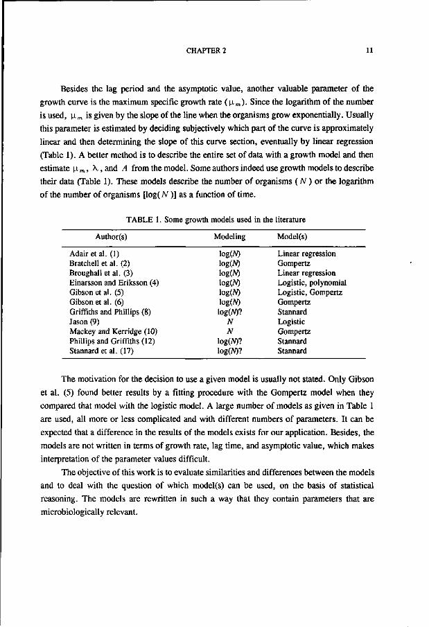
TABLE 1. Some growth models used in the literature
Author(s)
Adair et al. (1) Bratchellet al. (2) Broughall et al. (3) Einarsson and Eriksson (4) Gibson et al. (5) Gibson et al. (6) Griffiths and Phillips (8) Jason (9) Mackey and Kerridge (10) Phillips and Griffiths (12) Stannard et al. (17)
Modeling
log(A0 logW) log(A0 log(A0 log(JV) log(N) log(A0?
N N
logWJ? log(N)?
Model(s)
Linear regression Gompertz Linear regression Logistic, polynomial Logistic, Gompertz Gompertz Stannard Logistic Gompertz Stannard Stannard
The motivation for the decision to use a given model is usually not stated. Only Gibson
et al. (5) found better results by a fitting procedure with the Gompertz model when they
compared that model with the logistic model. A large number of models as given in Table 1
are used, all more or less complicated and with different numbers of parameters. It can be
expected that a difference in the results of the models exists for our application. Besides, the
models are not written in terms of growth rate, lag time, and asymptotic value, which makes
interpretation of the parameter values difficult.
The objective of this work is to evaluate similarities and differences between the models
and to deal with the question of which model(s) can be used, on the basis of statistical
reasoning. The models are rewritten in such a way that they contain parameters that are
microbiologically relevant.

12 BACTERIAL GROWTH CURVE MODELING
THEORY
Description of the bacterial growth curve. Since bacteria grow exponentially, it is
often useful to plot the logarithm of the relative population size [ y = ln(N /N „)] against
time (Fig. 1). The three phases of the growth curve can be described by three parameters: the
maximum specific growth rate, [i m, is defined as the tangent in the inflection point; the lag
time, X., is defined as the x-axis intercept of this tangent; and the asymptote [ A =
l n (A/ . /N 0 ) ] is the maximal value reached. Curves may show a decline. This kind of
behavior is called the death phase and is not considered in this chapter.
TABLE 2. Models used an their modified forms
Equation (y=)
Logistic: a
[1 + exp(b - ex)]
Gompertz:
a e x p [ - e x p ( b - e x ) ] A
Modified equation* (y=)
A
( l + e x p [ ^ ( \ - 0 + 2]}
e x p < - e x p ^V-o+i >
Richards:
a { l + uexp[ /c (T-x) ]}" A\ 1+ uexp(1+ u)exp —( i + vy " ( \ - o
Stannard:
al1+exp (Z+fcx)
A{ 1 + uexp( 1 +i;)exp ^ ( i + ü ) l , * : J ( \ - 0
Schnute: . , . . , l - e x p [ - a ( t - T , ) ] ^ w t
1-Ö l - 6 e x p ( a \ + l-b-at)
' e=exp(l); v = shape parameter.
Reparameterization of the growth models. Most of the equations describing a
sigmoidal growth curve contain mathematical parameters ( a , ö , c,...) rather than parameters
with a biological meaning (A,\in, and \ ) . It is difficult to estimate start values for the
parameters if they have no biological meaning. Moreover, it is difficult to calculate the 95%
confidence intervals for the biological parameters if they are not estimated directly in the
equation but have to be calculated from the mathematical parameters. Therefore, all the
growth models were rewritten to substitute the mathematical parameters with A, [im, and

CHAPTER 2 13
X. This was done by deriving an expression of the biological parameters as a function of the
parameters of the basic function and then substituting them in the formula. As an example,
we show here the modification of the Gompertz equation, which is written as:
y = a • e xp [ - exp (b -ct)] (1)
To obtain the inflection point of the curve, the second derivative of the function with respect
to t is calculated:
d y
dzy
dt
, 2 .
= ac- e x p [ - e x p ( b - c O ] - e x p ( b - c t ) (2)
_ ac e x p [ - exp (b -ct)]- exp(b -ct)- [ exp(b -ct)- 1] (3) d r
At the inflection point, where t = t-,, the second derivative is equal to zero:
- 0 -» t{ = b/c (4) d2y
dt'
Now an expression for the maximum specific growth rate can be derived by calculating the
first derivative at the inflection point.
(dy\ ac
The parameter c in the Gompertz equation can be substituted for by c = \ime/a.
The description of the tangent line through the inflection point is:
y = Um-<+ f -Hm'i (6)
The lag time is defined as the f-axis intercept of the tangent through the inflection point:
0 = \im-X + --\imti (7)

14 BACTERIAL GROWTH CURVE MODELING
Using equations 4, 5, and 7 yields:
, ( b - 1 ) x = —— (8)
The parameter b in the Gompertz equation can be substituted for by:
Ö - — \+\ (9)
The asymptotic value is reached for t approaching infinity:
£->«>: y ->a =» y4 = a (10)
The parameter a in the Gompertz equation can be substituted for by A, yielding the
modified Gompertz equation:
y = Aexpi-exp — ( \ - 0 + 1 (11)
The models with four parameters also contain a shape parameter ( v ) . Table 2 shows the
results for all equations used in this chapter.
TABLE 3. Selection of models based on Schnute (16)
Values of a and b
a > 0, b = 0
a > 0, b < 0
a > 0, b = -1
a = 0, Z> = 1
a = 0, * = 0.5
a = 0, b = 0
a < 0, b = 1
Model
Gompertz
Richards
Logistic
Linear
Quadratic
rth power
Exponential
No. of parameters
3
4
3
2
2
2
3

CHAPTER 2 15
The modified Stannard equation appears to be the same as the modified Richards
equation. The parameters a and b in the Schnute equation are retained in the modified Schnute
equation because they may be used for model selection (Table 3). However, substitution of a
and b in the Schnute equation would result in the modified Richards equation.
Broughall et al. (3) used the Verhuist differential equation (resulting in a logistic curve)
at times greater than the lag time and used N = N 0 if the time was smaller than the lag time.
This relation has no smooth transition from a lag phase to a growth phase. Since all our
growth data show such a smooth transition this model was not considered.
100 120 140 160 180 time (h)
FIG. 2. Growth curve of L. plantarum at 18.2°C fitted with the Gompertz ( ) and Richards ( ) models.
Fitting of the data. The nonlinear equations were fitted to growth data by nonlinear
regression with a Marquardt algorithm (11,13). This is a search method to minimize the sum
of the squares of the differences between the predicted and measured values. The program
automatically calculates starting values by searching for the steepest ascent of the curve
between four datum points (estimation of n m ) , by intersecting this line with the x axis
(estimation of A.), and by taking the final datum point as estimation for the asymptote (A).
The algorithm then calculates the set of parameters with the lowest residual sum of squares
(RSS) and their 95 % confidence intervals.

16 BACTERIAL GROWTH CURVE MODELING
Model comparison. One way to discriminate among models is to compare them
statistically. In that case, the RSS alone does not give enough information because different
models can have a different number of parameters. Models with a greater number of
parameters usually give a lower RSS. A better method is to determine whether it is
worthwhile to use more parameters to lower the RSS. Therefore, data fits obtained by using
the various models were compared statistically by the use of the t test and the F ratio test.
t test. First, the data were fitted by the Schnute model and parameters a and b were
evaluated. The Schnute model is a comprehensive model; it encompasses all of the other
simpler models. This is shown in Table 3, in which values of the Schnute parameters a and
b are given, leading to one of the other models. The 95 % confidence intervals of the different
parameters were calculated with the value given by the Student t test. If, for instance, a value
of zero is in the 95% confidence interval of b (and a > 0), the Gompertz model is suitable
(Table 3).
\n{N/No)
24 28 time (h)
FIG. 3. Growth curve of L. plantarum at 35.0°C fitted with the Gompertz ( ) and Richards ( ) models.
F test. The logistic, Gompertz, Richards, and Schnute models were used to fit the data,
and the RSS was calculated. Under the assumption that the four-parameter Schnute model
exactly predicts the number of organisms, the RSS of the Schnute model was taken as an
estimate of the measuring error. Whether a three-parameter model would be sufficient to

CHAPTER 2 17
describe the data could then be validated with an F test. In this test, the difference between
the RSS values for the three- and four-parameter models was compared to the RSS of the
four-parameter model. The difference in RSS of the three- and the four-parameter models is
the profit we get from adding one parameter. If this profit is much smaller than the measuring
error, as determined from the four-parameter model, adding the extra parameter is not
worthwhile, as it would not be observable. If, however, this profit is much greater than the
measuring error, it is worthwhile to add the extra parameter. The following is then calculated:
ƒ = R S S / D F t es ted aga ins t FDFi (12)
where RSS! is the RSS from the Schnute model, RSS2 is the RSS from the three-parameter
model, DFj is the number of degrees of freedom from the Schnute model and equals the
number of datum points (npoints) - 4, and DF2 is the number of degrees of freedom from the
three-parameter model and equals npoints - 3. Note that DF2 - DF, = 1, so the F test becomes:
RSS 2 -RSS! . ƒ = tested aga ins t Fnr (13) J RSS^DF! u DF' K3)
If the models were linear in their parameters, this ƒ value would be F-distributed under
the assumption that the four-parameter model is correct. Even for nonlinear models, the
variance ratio shown above is approximately F-distributed when the sample size is large (16).
This analysis is an approximation at best, and this procedure should be considered an informal
process, rather than a rigorous statistical analysis, because of the use of nonlinear models
(16). In some boundary cases, the Student t test and the F test can therefore give contradictory
results.
MATERIALS AND METHODS
In 40 experiments, Lactobacillus plantarum (American Type Culture Collection
[ATCC]-identified; no ATCC number) was cultivated in MRS medium (Difco Laboratories)
at different temperatures. Growth was measured with plate counts on pour plates (MRS
medium with 12 g of agar [Agar technical; Oxoid Ltd.] per liter). The inoculation level was
0.01% (about 5 10s organisms).

18 BACTERIAL GROWTH CURVE MODELING
Growth data of Candidaparapsilosis, Pseudomonas putida, Enterobacter agglomérons,
a Nocardia sp., Salmonella Heidelberg, Staphylococcus aureus, and Listeria monocytogenes
were kindly provided by J.P.P.M. Smelt, C.J.M. Winkelmolen, P. Breeuwer, and F.G.C.T.
Sommerdijk.
60 time (h)
FIG. 4. Growth curve of L. plantarum at 18.0°C fitted with the Gompertz ( ) and Richards ( ) models.
RESULTS
All the models visually gave reasonably good fits of the data (Fig. 2 and 3, for
example). In some cases, the Schnute and Richards models gave some problems with the
fitting because the parameter estimates came in an area where the function predicted such a
large value that an overflow error resulted. The Gompertz and logistic models never gave
problems with fitting. In all cases, the RSS values for the Richards and Schnute models were
the same, which was expected because the models are basically the same.
Plate count data for L. plantarum. In Table 4, the results of the parameter estimation
for 40 sets of data are reported. In this table, the temperature at which the experiment was
conducted is given. With the use of the Student t test value, the 95 % confidence intervals for
the parameters a and b were calculated. The lower 95% confidence limit of the parameter a
is given in Table 4 to determine whether a = 0 is within the confidence interval. Furthermore,

CHAPTER 2 19
TABLE 4. Statistical-analytical data for 40 growth curves of L. plantarum
reo
6.0 6.1 8.3 8.6
12.0 12.2 15.1 15.2 18.0 18.2 18.2 18.2 18.6 21.5 21.5 25.0 25.0 28.4 28.6 32.0 32.0 32.4 34.9 35.0 35.3 36.6 37.9 38.4 40.0 41.4 41.5 41.5 41.8 41.9 42.1 42.2 42.6 42.8 42.8 42.8
a • ' b
min
0.003 -0.0006 0.011 0.008 0.024 0.023 0.049 0.049 0.065 0.059 0.076 0.068
-0.607 -0.322 0.092 0.116 0.082 0.259 0.252 0.257 0.260 0.272 0.301 0.255 0.257 0.262 0.245 0.264 0.247 0.151 0.043 0.070
-0.278 -1.01 0.156 0.014
-0.101 -7.82 0.315
-0.061
b • abc
-0.988 -1.18 -0.113 -0.748 -0.247 -0.337 -0.786 -0.096 -0.086 -4.23 -0.058 -0.192 -4.72 -2.04 -0.167 -0.317 -0.147 -0.676 -0.352 -1.06 -0.933 -0.276 -0.544 -0.314 -0.320 -0.207 -0.299 -0.870 -1.73 -1.26 -0.220 -0.403 -0.641 -4.50 -0.152 -0.355 -0.443
-52.1 -1.09 -2.20
b "b
''max
0.994 1.98 0.435 0.470 0.548 0.672 0.289 0.501 0.540 0.275 0.471 0.350 6.39 2.89 0.614 0.786 0.970 0.201 0.183 0.432 0.367 0.328 0.421 0.623 0.455 0.635 0.676 0.487 0.391 0.713 0.855 1.26 1.69 5.40 0.726 1.46 2.44
46.0 0.824 1.61
ƒ"
Gom
0.001 0.194 1.91 0.204 0.577 4.10 0.875 1.80 7.84 1.45 3.78 0.301 1.99 0.277 1.05 3.10 2.44 1.69 0.481 1.06 1.33 0.035 0.099 0.510 0.136 1.08 0.604 0.469 2.65 0.416 5.18 1.06 0.899 0.464 3.31 1.93 3.20 1.79 0.083 0.084
Log
0.078 1.49
53.6 4.21
18.4 40.6 5.03
46.2 49.9 0.485
60.4 30.0 6.35 2.50
19.2 23.8 16.8 10.0 34.5 2.71 4.85
32.4 13.3 17.0 21.1 22.2 15.4 5.11 0.382 1.65
29.1 6.45 4.76 1.49
26.8 6.15 6.11 0.395 2.63 0.527
F
table
4.13 4.75 4.21 4.33 4.36 4.97 4.45 4.84 4.60 4.75 4.84 4.31 6.60 5.99 4.75 4.97 4.84 4.84 4.84 4.97 5.59 4.84 5.59 4.97 4.75 4.67 4.60 5.99 4.84 5.12 4.75 4.75 6.60 7.72 4.67 4.67 6.60 5.12 4.75 5.12
Gom
1.70 0.282 0.707 1.09 1.13 0.424 1.06 0.375 0.611 1.39 0.233 0.516 0.155 0.486 0.648 0.800 1.07 0.430 0.210 0.883 0.334 0.241 0.200 0.482 0.471 0.722 0.880 0.229 1.17 0.668 0.331 1.57 0.209 0.844 0.400 1.47 0.633 0.633 0.141 0.105
RSS
Logf
1.70 0.312 1.97 1.30 2.11 1.56 1.30 1.67 2.02 1.29 1.12 1.20 0.252 0.658 1.55 2.07 2.21 0.714 0.833 1.01 0.475 0.948 0.571 1.24 1.28 1.81 1.77 0.394 0.974 0.756 0.792 2.22 0.346 1.04 0.975 1.89 0.858 0.551 0.171 0.110
Richards
1.70 0.277 0.660 1.08 1.10 0.300 1.00 0.322 0.391 1.24 0.173 0.509 0.111 0.464 0.596 0.611 0.876 0.373 0.201 0.798 0.281 0.240 0.197 0.459 0.466 0.667 0.844 0.213 0.941 0.638 0.231 1.44 0.178 0.757 0.319 1.28 0.386 0.528 0.140 0.104
a a and b are Schnute parameters;b min and max are 95% confidence limits;c Boldface data indicate acceptance of logistic model with f test;d Boldface data indicate acceptance of given model with F test; f Boldface data indicate that RSS with Gompertz model is greater than RSS with logistic model.
the 95% confidence limits for b are given. Comparing the confidence intervals in Table 4 for
b with Table 3 results in Table 5. In Table 3, we can see that if b = 0, the Schnute model
changes into the Gompertz model, so we accepted the Gompertz model if the value of zero

20 BACTERIAL GROWTH CURVE MODELING
was within the 95% confidence interval of b. This was true in all cases (Table 4), so the
Gompertz model, although a three-parameter model, was accepted in all cases by the t test.
Furthermore, the/-testing values for the Gompertz and the logistic models and the F table
values are given in Table 4. With the use of the F test, the difference between the RSS values
for the three- and four-parameter models was compared to the RSS of the four-parameter
model. For the Gompertz model, the/-testing value was lower than the F table value in all
but two cases (Table 4).
TABLE 5. Determination of models for L. plantarum based on the method of Schnute (16)
Values of a and b
a > 0, b = 0 a > 0, * < 0 a > 0, * = -1 a = 0, b = 1 a = 0, b = 0.5 a = 0,b = 0 a < 0, b = 1
Model
Gompertz Richards Logistic Linear
Quadratic fth power
Exponential
No. (% of total)' of results accepted with:
f test
40(100) 40(100) 11 (28) 8(20) 8(20) 8(20) 8 (20)
F test
38(95)
17(43)
* Total number of experiments = 40.
In the cases in which the F test favored the Richards model over the Gompertz model
(Fig. 4 and 5), the differences between the two models were still very small. The logistic
model, however, was accepted by the t test only 11 times (out of 40) and by the F test 17
times (Table 4).
In addition, the RSS values of the Gompertz, logistic, and Richards models are given
in Table 4. The RSS values for the four-parameter models were always lower than the RSS
values for the three-parameter models. In only three cases, the logistic model gave a lower
RSS value than the Gompertz model (Table 4; Fig. 6), but in these cases the Gompertz model
still fitted the data acceptably.
In Fig. 7, the confidence intervals for the parameter b (Schnute model with the t test)
are shown. In this graph, it can be seen that the value of zero (Table 3, Gompertz model) was
always within the confidence interval; however, the value of-1 (Table 3, logistic model) was
much less frequently within the confidence interval (only 11 times).
In Fig. 8, the results from the F test for the Gompertz model are shown. The squares
represent the /-testing values, and the pluses represent the critical F table values (95 %

CHAPTER 2 21
8 10 12 time (h)
FIG. 5. Growth curve of L. plantarum at 41.5°C fitted with
the Gompertz ( ) and Richards ( ) models.
ln(A//A/o) 8
8 12 16 20 24 time (h)
FIG. 6. Growth curve of L. plantarum at 40.0°C fitted with
the Gompertz ( ) and logistic ( ) models.

22 BACTERIAL GROWTH CURVE MODELING
confidence). If the /-testing value was smaller than the F table value, the three-parameter
model was accepted. In this graph, it can be seen that the Gompertz model was rejected only
2 times out of 40 (5%). This 5% rejection level may be expected with a 95% confidence level.
TABLE 6.
Orgai
Statistical-
lism
analytical data for 27 growth curves
n ab h abc h ab fi min min max J
Gom
of organisms
Log
F
table
other than L. plantarum
Gom
RSS
Logf Rich
Candida parapsilosis 0.038 -1.60 0.761 1.71 1.11 10.1 0.114 0.100 0.073 C. parapsilosis 0.136 -1.12 0.154 6.67 4.86 10.1 0.086 0.070 0.027 C. parapsilosis 0.039 -1.60 1.16 0.071 1.07 10.1 0.102 0.135 0.100 C. parapsilosis 0.117 -0.673 0.751 0.557 21.1 10.1 0.030 0.205 0.025 C. parapsilosis -0.071 -3.68 1.70 3.22 0.000 10.1 0.362 0.175 0.175 Pseudomonas putida 0.050 -2.42 -0.513 18.7 1.08 4.17 4.47 2.86 2.76 P.putida 0.027 0.114 1.12 3.84 15.3 4.17 6.42 8.60 5.70 P. putida 0.059 -0.169 0.701 1.25 16.2 4.13 3.98 5.66 3.83 P.putida 0.037 -0.174 1.54 6.31 17.5 4.16 11.9 15.4 9.85 Enterobacter agglomérons 0.002 0.141 1.10 15.2 41.5 4.14 13.4 20.7 9.19 E. agglomerans 0.015 0.412 0.802 26.7 111 4.17 4.87 12.1 2.58 E. agglomerans 0.020 0.240 0.793 9.26 48.8 4.13 5.07 9.70 3.98 E. agglomerans 0.025 0.432 1.01 17.7 59.9 4.15 7.80 14.4 5.03 Nocardia sp. 0.072 -2.08 1.29 0.540 1.21 5.12 0.176 0.188 0.166 Salmonella Heidelberg -3.18 -10.9 12.9 0.720 1.43 161 1.23 1.74 0.717 Staphylococcus aureus 0.178 -0.759 1.82 0.843 3.86 6.61 0.526 0.798 0.450 S. aureus 0.009 -3.73 5.39 15.2 42.5 6.61 0.543 1.28 0.134 S. aureus -2.13 -3.39 5.39 1.25 1.73 6.61 1.87 2.01 1.49 S. aureus -3.60 -5.07 7.07 1.28 1.56 6.61 0.886 0.926 0.706 S. aureus -0.529 -2.11 4.09 2.86 4.66 6.61 4.54 5.58 2.89 S. aureus -0.315 -4.67 6.44 1.51 3.31 6.61 0.807 1.03 0.620 S. aureus 0.062 0.235 1.77 10.8 21.6 10.1 1.12 1.99 0.243 S. aureus 0.094 -0.056 2.06 14.4 29.6 10.1 0.873 1.63 0.151 S. aureus 0.452 0.747 1.25 3.44 5.31 10.1 0.273 0.353 0.127 S. aureus 0.066 -0.512 1.87 2.62 8.59 10.1 0.628 1.29 0.335 S. aureus -0.060 -1.66 1.81 0.094 3.20 18.5 0.031 0.078 0.030 Listeria monocytogenes -16.5 -171 172 0.000 0.136 18.5 0.007 0.007 0.007
* a and b are Schnute parameters;b min and max are 95% confidence limits;c Boldface data indicate acceptance of logistic model with t test;d Boldface data indicate acceptance of given model with F test; 'Boldface data indicate that RSS with Gompertz model is greater than RSS with logistic model.
Plate count data for other organisms. While it could be that only L. plantarum growth
data are described well by the Gompertz model, the same comparison of models was carried
out with growth data from other microorganisms (Tables 6 and 7). With these data, the
Gompertz model was accepted in 70% of the cases by the t test (b=0 within the confidence

CHAPTER 2 23
b 10
8
6
4
2
0
-2-
-4
-6-
-8
-10
am IlI»l3!l]Hl! 1« S wjg
10 20 30 40 Exp. No.
FIG. 7. è confidence intervals of L. plantarum growth data fitted with the Schnute model (16). Exp. No., Experiment number.
F and f values 8
7
6
5
4
3
2
1
K + + + + + + L. + + + + + + + n
10 20 30 40 Exp. No.
FIG. 8. Results of an F test of L. plantarum growth data.
The Gompertz and Richards models are compared, •ƒ value, *F value.

24 BACTERIAL GROWTH CURVE MODELING
interval) and in 67% of the cases by the F test. The logistic model was accepted in 52% of
the cases by the t test (b = -1 within the confidence interval) and in 59% of the cases by the
F test.
TABLE 7. Determination of models for organisms other than L. plantarum based on the method of Schnute (16)
Values of a and b
a > 0, b = 0 a > 0, b < 0 a > 0, b = -1 a = 0, b = 1 a = 0, * = 0.5 a = 0, b = 0 a< 0,b= 1
Model
Gompertz * Richards Logistic Linear Quadratic fth power Exponential
No. (% of total)" of results
ftest
19(70) 20(74) 14(52) 8(30) 8(30) 8(30) 8(30)
accepted with:
Ftest
18(67)
16(59)
* Total number of experiments = 27.
DISCUSSION
In order to build models to describe the growth of microorganisms in food, it is
necessary to measure growth curves. To reduce the measured data to interesting parameters
such as the growth rate, it is recommended that the data be described with a model instead of
by using linear regression over a subset of the data. Sigmoidal models to describe the growth
data can be constructed with three or four parameters.
We compared several models statistically and found that, for L. plantarum, the
Gompertz model was accepted in all cases by the t test and was accepted in 95% of the cases
by the F ratio test; therefore, the Gompertz model can be regarded as sufficient to describe
the growth curves of L. plantarum. The logistic model, however, seems not to be sufficient
to describe the data. It was accepted in 28% of the cases by the / test and in 43% of the cases
by the F test with L. plantarum.
With the data of other microorganisms, the Gompertz model was accepted in 70% of
the cases. With the data of the other organisms, the logistic model was accepted in 52% of
the cases with the t test and in 59% of the cases with the Ftest. Linear, quadratic, rth-power,
and exponential models were accepted in very few cases. Therefore, we can conclude that all
growth curves are better fitted with the Gompertz model than with logistic, linear, quadratic,
rth-power, and exponential models.

CHAPTER 2 25
In some cases, the confidence interval of the Schnute parameter b (bmia- b^) was very
large. In these cases, there were not enough data to describe all three growth phases.
Therefore, the confidence level of the resulting parameters is not very high. These sets of data
are not very suitable for the estimation of parameters.
In a number of cases, the four-parameter Schnute model was statistically better than the
Gompertz model (P. putida and E. agglomerans). These growth curves contained a very large
number of datum points (34 to 38) and with such a large number of datum points the
difference in degrees of freedom between three- or four-parameter models is not important
(with 34 datum points: 31 degrees of freedom for Gompertz or 30 degrees of freedom for
Richards). For the other organisms (C. parapsilosis and S. aureus), the Gompertz model was
accepted in most cases. For the growth curves of the Nocardia sp., Salmonella Heidelberg,
and L. monocytogenes, the Gompertz model was accepted in all the cases, but only one curve
for these organisms was used.
The three-parameter models gave no difficulties in finding the least-square parameters.
In almost all the cases, the Gompertz model can be regarded as the best model to describe the
growth data. If a three-parameter model is sufficient to describe the data, it is recommended
over a four-parameter model because the three-parameter model is simpler and therefore
easier to use and because the three-parameter solution is more stable since the parameters are
less correlated. Moreover, when a three-parameter model is used, the estimates have more
degrees of freedom, which can be important when a growth curve with a small number of
measured points is used. Furthermore, it is very important that all three parameters can be
given a biological meaning. The fourth parameter in the four-parameter models is a shape
parameter and is difficult to explain biologically.
In a number of cases (especially when a large number of datum points are collected), a
four-parameter model can be significantly better; therefore, it is recommended that the
procedure given in this chapter be carried out with a number of sets of data in order to find
out the best model to describe the specific sets of data.
ACKNOWLEDGMENTS
This work was partly supported by Unilever Research Laboratorium Vlaardingen. We thank P.M. Klapwijk, J.P.P.M. Smelt, and H.G.A.M. Cuppers for valuable discussions and H.H. Beeftink for reading the manuscript.

26 BACTERIAL GROWTH CURVE MODELING
REFERENCES
1. Adair, C , D.C. Kilsby, and P.T. Whittall. 1989. Comparison of the Schoolfield (non-linear
Arrhenius) model and the square root model for predicting bacterial growth in foods. Food
Microbiol. 6:7-18.
2. Bratchell, N., A.M. Gibson, M. Truman, T.M. Kelly, and T.A. Roberts. 1989. Predicting
microbial growth: the consequences of quantity of data. Int. J. Food Microbiol. 8:47-58.
3. Broughall, J.M., P.A. Anslow, and D.C. Kilsby. 1983. Hazard analysis applied to microbial
growth in foods: development of mathematical models describing the effect of water activity.
J. Appl. Bacteriol. 55:101-110. 4. Einarsson, H., and S.G. Eriksson. 1986. Microbial growth models for prediction of shelf life
of chilled meat, p. 397-402. In Recent advances and developments in the refrigeration of meat
by chilling. Institut International du Froid-International Institute of Refrigeration, Paris.
5. Gibson, A.M., N. Bratchell, and T.A. Roberts. 1987. The effect of sodium chloride and
temperature on the rate and extent of growth of Clostridium botulinum type A in pasteurized
pork slurry. J. Appl. Bacteriol. 62:479-490.
6. Gibson, A.M., N. Bratchell, and T.A. Roberts. 1988. Predicting microbial growth: growth
responses of salmonellae in a laboratory medium as affected by pH, sodium chloride and storage
temperature. Int. J. Food Microbiol. 6:155-178.
7. Gompertz, B. 1825. On the nature of the function expressive of the law of human mortality,
and on a new mode of determining the value of life contingencies. Philos. Trans. R. Soc.
London 115:513-585.
8. Griffiths, M.W., and J.D. Phillips. 1988. Prediction of the shelf-life of pasteurized milk at
different storage temperatures. J. Appl. Bacteriol. 65:269-278.
9. Jason, A.C. 1983. A deterministic model for monophasic growth of batch cultures of bacteria.
Antonie van Leeuwenhoek J. Microbiol. Serol. 49:513-536.
10. Mackey, B.M., and A.L. Kerridge. 1988. The effect of incubation temperature and inoculum
size on growth of salmonellae in minced beef. Int. J. Food Microbiol. 6:57-65.
11. Marquardt, D.W. 1963. An algorithm for least-squares estimation of nonlinear parameters. I.
Soc. Ind. Appl. Math. 11:431-441.
12. Phillips, J.D., and M.W. Griffiths. 1987. The relation between temperature and growth of
bacteria in dairy products. Food Microbiol. 4:173-185.
13. Press, W.H., B.P. Flannery, S.A. Teukolsky, and W.T. Vetterling. 1988. MRQMIN , p.
772-776. In Numerical recipes. Cambridge University Press, Cambridge.
14. Richards, F.J. 1959. A flexible growth function for empirical use. J. Exp. Bot. 10:290-300.
15. Ricker, W.E. 1979. Growth rates and models. Fish Physiol. 8:677-743.
16. Schnute, J. 1981. A versatile growth model with statistically stable parameters. Can. J. Fish.
Aquat. Sei. 38:1128-1140.
17. Stannard, C.J., A.P. Williams, and P.A. Gibbs. 1985. Temperature/growth relationship for
psychrotrophic food-spoilage bacteria. Food Microbiol. 2:115-122.
CHAPTER 3
COMPARISON OF DEFINITIONS OF THE LAG PHASE AND THE EXPONENTIAL PHASE IN BACTERIAL GROWTH
ABSTRACT
Different definitions of the lag time and of the duration of the exponential phase can be
used to calculate these quantities from growth models. The conventional definitions were
compared with newly proposed definitions. It appeared to be possible to derive values for the
lag time and the duration of the exponential phase from the growth models, and differences
between the various definitions could be quantified. All the different values can be calculated
from the growth parameters n m , X., and A. Therefore, it appeared to be unnecessary to use
complicated mathematical equations: simple equations were adequate. For the Gompertz
model the conventional definition of the lag time did not differ appreciably from the newly
proposed definition. The end-point of the exponential phase and thus the duration of the
exponential phase differed considerably for the two definitions. For the logistic model the two
definitions lead to considerable differences for all quantities. It is recommended that the
conventional definition is used for calculating the lag time. For the duration of the exponential
phase it is recommended that the new definition is used. The value can be calculated,
however, directly from the conventional growth parameters.
INTRODUCTION
In predictive microbiology, models are used to describe the growth of micro-organisms
under different environmental conditions. In order to build these models growth has to be
measured and modelled. Bacterial growth often shows a phase in which the growth starts from
a zero rate and then accelerates to a maximal value ( p. m) in a certain period of time, resulting
in a lag time ( X. ). In addition, growth curves contain a final phase in which the rate decreases
This chapter has been published as:
Comparison of Definitions of the Lag Phase and the Exponential Phase in Bacterial Growth
M.H. Zwietering, F.M. Rombouts, K. van 't Riet (1992)
J. Appl. Bacteriol. 72:139-145

28 LAG PHASE DEFINITIONS
and finally reaches zero, so that an asymptotic level (A) is reached. The bacterial growth
curve can be described with, e.g. the Gompertz and logistic growth models. Using these
models the parameters \x.m, X, and A can be estimated from growth data (2, 4). The most
common way of calculating the duration of the lag time ( X. ) is extrapolation of the tangent at
the inflection point of the growth curve, back to the inoculation level (Fig. 1). After this lag
phase the exponential phase sets in. The end of this exponential phase ( a ) can be defined as
the time at which the extrapolation of the tangent in the inflection point reaches the final level
(Fig. 1). Buchanan and Cygnarowisz (1) proposed a new definition for calculating the lag time
in bacterial growth by deriving the time at which the change of the growth rate is maximal
(maximum acceleration of the growth rate). This is given as the time at which the third
derivative of the logarithm of the number of organisms with respect to time is zero (Fig. 2).
This is an interesting new way of defining the lag time. Moreover, the duration of the
exponential phase can be calculated with the same definition, as the difference between the
times of maximum acceleration and maximum deceleration, i.e. the time between two zero
values of the third derivative.
In(WAfo)
time FIG. 1. A growth curve with the parameters nm (specific growth rate), ks (lag time), ag (end of exponential phase), and A (asymptote). ^„ is determined as the time where the tangent crosses the
starting level, a, is determined as the time where the tangent crosses the final level.

CHAPTER 3 29
The determination of the lag phase will be of most interest in the modelling of the
growth of food-borne pathogens. Duration of the exponential growth will be more relevant
for the modelling of the growth of spoilage organisms, and for defining the growth state of
the organisms.
The object of this work was to evaluate differences between different definitions of the
lag time, and the duration and the end of the exponential phase.
THEORY
Different definitions of the lag phase. Using a description of the growth curve like the
Gompertz or logistics equations, the third derivative can be derived from these equations.
Like Buchanan and Cygnarowisz (1) we adopted the form of the Gompertz equation, as used
by Gibson et al. (2):
y ( 0 = ß + C e x p { - e x p [ - ß ( t - M ) ] } (1)
where: y(t) = log10 count at time t,D = log number at t= - ° ° , C = final log increase in
bacterial numbers, M = time at which culture achieves its maximum growth rate (h),
B = relative growth rate at time M (l/h), t = time (h).
If we use: $ = exp[-B(t-M)] (2)
we get for the Gompertz equation:
y ( t ) = Z? + C e x p ( - * ) (3)
Using: ~dt=~ W
the subsequent derivatives may be calculated as:
dy — = 5C*exp(-<t>) (5)
y = S2C*(*-l)exp(-*) (6)

30 LAG PHASE DEFINITIONS
log(W) 10-
8-
6-
4-
2-
n -u
-2
J
v/ / V'
, .']
\ / \ /
20 40 60 80 100 time (h)
-) with 0=2 . 3 , fl=0.095, C=8.1, and M= 20.8; the third FIG. 2. The Gompertz function (-
derivative (1000*, ), the newly proposed lag time (X. 6 ) and end of the exponential phase
(a6 ). Kb is determined as the time where the third derivative is zero, a t is determined as the time
where the third derivative is zero for the second time, a , is determined as the time where the
tangent ( ) crosses the final level.
\og(N) 6
-
• * * * " — " * * * *"""
\ S \ \
X N
— I 1 1 1 1 1 1 1 1 1 1 1 1 1 1 r*-! r*~i
12 16 20 time (h)
FIG. 3. Beginning of the Gompertz function ( ) with £>=2.3, 5=0.095, C=8.1, and
Af=20.8. \g is determined as the time where the tangent ( ) crosses the starting level, xb is
determined as the time where the third derivative (1000*, ) is zero.

CHAPTER 3 31
dt ^f = B3C<i>(<i>2-3<i> + l ) e x p ( - * ) (7)
The Gompertz equation and its third derivative are shown in Fig. 2. In Fig. 3 the beginning
of the Gompertz function is given.
The lag time ( X b ) is now defined as the smallest r-value for which this third derivative
is equal to zero (1). The factors 4> and exp ( - * ) on the right hand side of equation 7 cannot
equal zero. This results in:
e x p [ - 2 ß ( t - M ) ] - 3 e x p [ - ß ( t - M ) ] + 1 =0 (8)
This can be rewritten as:
e x p [ - B ( J - M ) ] - e x p -f(*-Af) ]-}{ exp[- /?(«- M)] + exp - - ( f - M ) 1 = 0 (9)
Buchanan and Cygnarowisz (1) used this equation to calculate the two zero values of
the third derivative of the Gompertz function. They used a root-finding procedure to calculate
where one of the two parts of equation 9 is zero. However, equation 8 is a simple quadratic
equation, and can thus be solved analytically:
$'-3<t> + 1 =0 (10)
The two solutions are obtained from:
<exp[ -Ä( t -M)]> I > 2 -3 ± V 9 - 4
, . 1. f 3 ± v 5 t i . 2 - M - - l n '
(11)
(12)
Since the lag time is the root with the smallest time the definition of Buchanan and
Cygnarowisz (1) gives the lag time ( X „ ) as:
. . . 1, f 3 + ^ .. 0.96 ^ h = M - — I n = M —
* B [ 2 J B (13)

32 LAG PHASE DEFINITIONS
The conventional way of defining the lag time ( \ ) results in the following equation (2):
K-M-B (14)
Equations 13 and 14 show that there is little numerical difference between the two definitions
of the lag time.
RESULTS
Comparison of different definitions of the lag phase. The various definitions of the
lag time are compared quantitatively in Table 1, by using the parameter values (D, B, C, M)
of Buchanan and Cygnarowisz (1) and calculating the values of the different lag times. Each
parameter is also doubled and halved to describe the effects in a wider range of parameters.
TABLE 1. Comparison of lag time estimates
Gompertz parameters
D
2.30
1.15
4.60
2.30
2.30
2.30
2.30
2.30
2.30
2.30
B
0.095
0.095
0.095
0.0475
0.190
0.095
0.095
0.095
0.095
0.095
C
8.10
8.10
8.10
8.10
8.10
4.05
16.2
8.10
8.10
8.10
M
20.8
20.8
20.8
20.8
20.8
20.8
20.8
41.6
10.4
10.0
Calculated values
nm
0.283
0.283
0.283
0.142
0.566
0.142
0.566
0.283
0.283
0.283
G.T.
1.063
1.063
1.063
2.127
0.532
2.127
0.532
1.063
1.063
1.063
K
10.27
10.27
10.27
-0.253
15.54
10.27
10.27
31.07
-0.126
-0.526
x.„
10.67
10.67
10.67
0.538
15.74
10.67
10.67
31.47
0.269
-0.131
D, B, C, M, Gompertz parameters; \im, specific growth rate (log count/h), equals BC/e; parameter values of Buchanan and Cygnarowisz (1) are used. Each parameter is also varied to describe the effects in a wider range of parameters; G.T. Generation time (h), equals log(2)e/ßC; \ s , conventional lag time (h), equals M - 1 /B ; \„ newly proposed lag time (h), equals M - 0.96/B .

CHAPTER 3 33
As can be seen in Table 1 there are no large numerical differences between the lag times
\ g and Kb. This can also be seen in Fig. 3, where the Kg and \ b are closely together.
Since the two definitions show no large differences, it is recommended that the conventional
definition (X„) is used, as this enables comparison to be made between values from the
literature. Moreover, equation 14 is easier to use and to incorporate into the Gompertz model
(4), although this could also be done for the newly proposed lag time. Table 1 shows more
parameter values resulting in negative values for the lag time, when using the conventional
definition (X-g). This could be an argument in favour of the newly proposed definition.
However, in these cases the differences between the two definitions also show small
deviations, which will be smaller than the measuring error of determining the lag time.
Therefore, in these cases it can be concluded that the lag time will be around zero with both
definitions. Equations 13 and 14 show that Kb and \ g can be easily recalculated. In
conclusion, it is not necessary to use the complicated third derivative numerical procedure if
A. is the only quantity of interest.
Buchanan and Cygnarowisz (1) also proposed that the end of the exponential growth
phase can be calculated as the point where the third derivative of the growth model becomes
zero for the second time (see Fig. 2). We call this the time a 6 :
• ( * ! ) a,-M U L J . H . ^ (15) L i,
" B B
Alternatively, the end of the exponential phase may be defined as the intersection
between the tangent in the inflection point of the growth curve and the final level (D+C, see
Fig. 2). This time a g can then be calculated with the description of this tangent (tangent
method, comparable to conventional definition of Kg):
BC C y = — - ( t - M ) + £> + - (16)
RC C D + C = — - ( a B - M ) + D + - (17)
.« 1 - 7 2 a 9 = M + — ( 1 8 )

(19)
34 LAG PHASE DEFINITIONS
Equations 15 and 18 show a significant numerical difference between the two a s . The
Gompertz curve is not symmetrical around the inflection point; the curvature at the beginning
of the curve is more pronounced than at the end, towards the stationary phase. Therefore, the
estimation of a g gives a higher value than the estimation using the definition of Buchanan
and Cygnarowisz (1). This can also be seen in Fig. 2.
e b , the duration of the exponential phase, can be calculated from equations 15 and 13
as:
l n ( ^ ) l n ( ^ ) 1 - 9 2
E L — Ott A, », — +
b b b B B B
and e g can be calculated from equation 18, and 14 as:
2 72 a a - ^ = — (20)
It can be seen that there is a large numerical difference between the two definitions of
the end of the exponential phase and, with that, also in the duration of the exponential phase.
However, e6 = 0.71 eg and therefore the e values always have the same ratio. Even so, the
end-points of the exponential phase a b and a g can be calculated if the growth parameters
are known. This makes the use of any of the two methods arbitrary. In Fig. 2 it can be seen
that for the tangent method, the growth behaviour at the predicted end of the asymptotic phase
already differs largely from exponential behaviour.
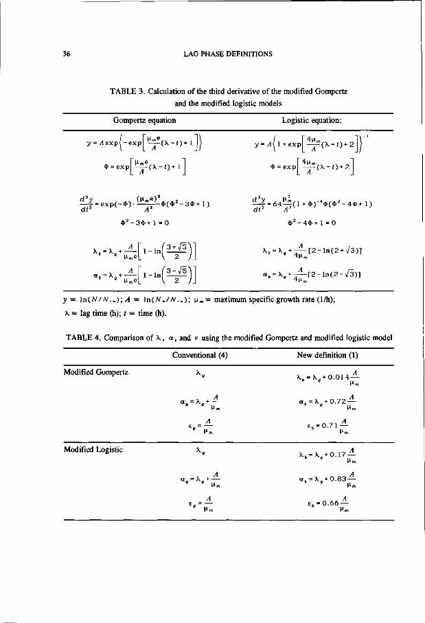
Comparison of different modifications of the Gompertz equation. Zwietering et al.
(4) modified the Gompertz equation, so that the growth parameters [im, X, and A are used
instead of mathematical parameters. Since they define a growth curve as \n(N / N .„)
versus time, the starting value of the logarithmic growth curve is equal to zero. Table 2 gives
a conversion table for the various definitions of the Gompertz model, used by Gompertz (3),
Gibson et al. (2), and Zwietering et al. (4).
For the modified Gompertz the third derivative can also be calculated (Table 3). With
this equation the newly defined lag time and end of the exponential phase can be calculated
and compared with the conventional definitions (Table 4). As the equation is written only in
a modified form, with the modified Gompertz model of Zwietering et al. (4) we get results
comparable with the Gompertz model used by Gibson et al. (2).

CHAPTER 3 35
TABLE 2. Conversion table of different Gompertz functions
Zwietenng et al. (4) nme nme Gompertz (3) b » X+ 1 ;c = ; a = A
A A
y = j4exp< - e x p ^ - 0 * 1 y - a e x p [ - e x p ( b - c ( ) ]
b - 1 Ac
Zwietering et al. (4) A vme Gibson et al. (2) M - \ + ;B - ——;D - 0 ;C= A
>l"i e y = / l e x p \ - e x p | — — ( K - f ) + l
y = D + C e x p { - e x p [ - B ( ( - M ) ] >
1 Pß
Gibson et al. (2) b = BM;c = B-,a = C Gompertz (3)
y - D + C e x p { - e x p [ - B ( f - M)]} < y - a e x p [ - e x p ( b - c l ) ]
b fi-c;M--;D-0;C-a
c
Buchanan and Cygnarowisz (1) proposed that their definition can also be used for other
growth models, such as logistic. For the modified logistic equation proposed by Zwietering
et al. (4) the third derivative is calculated (Table 3).
For the modified logistic model it can be seen in Table 4 and Fig. 4 that both the lag
time and the end of the exponential phase differ using the two different definitions. However,
with this equation the value of the lag time proposed by Buchanan and Cygnarowisz (1) can
also be calculated analytically from the values found with the modified logistic equation.
The various definitions of the lag time are compared quantitatively in Table 5 for the
Gompertz model, by using the parameter values (A, \s.m, and Kg ) and calculating the values
of the different lag times. Some of our own growth data of Lactobacillus plantation at
different temperatures are given by Zwietering et al. (5).
Some extreme cases are also used in which yl = l n ( 10 ' 0 ) = 23 as a maximum value
and A = 1 as a minimum value. A maximum value of the growth rate is calculated as a growth
rate with a generation time of 20 minutes: \im = 31n (2) (1/h). A minimum growth rate is
calculated as growth from 1 to 1010organisms during one year: \im = 24,365 = 0.0026 (1/h).
36 LAG PHASE DEFINITIONS
TABLE 3. Calculation of the third derivative of the modified Gompertz
and the modified logistic models
Gompertz equation Logistic equation:
y = /lexp< -exp Hme ( \ - < ) + l
* = exp H*.e
( x - O + 1
y - A( 1 + exp
4> = exp
4u„ • ( X . - 0 + 2
4u„ ( X - O + 2
—f- exp(-*) • — * ( * - 3 * + 1) dt3 A2
* ' - 3 * + 1 = 0
^-Ür = 6 4 ^ ) ( l +4>)_4<1>(*2-4<1>+ 1) dt3 A*
* ' - 4 * + 1 =0
Um«
A ^me
1 - I n
1 - I n
2 J.
3 - / 5
^„ = ^„ + 2—[2 - l n (2 + / 3 ) ]
a„ = \,, + — [ 2 - l n ( 2 - / 3 ) ]
v = ln(Af/iV_„); A = ln(W./iV_.); n m = maximum specific growth rate (1/h);
\ = lag time (h); f = time (h).
TABLE 4. Comparison of X., a, and e using the modified Gompertz and modified logistic model
Conventional (4) New definition (1)
Modified Gompertz K
<*t
K
<*.
-* .
- \
£ Ö =
- \
- \
E„ =
+ 0 . 0 1 4 —
+ 0 . 7 2 —
o.ziA
, + o . i / A ' Urn
+ 0 . 8 3 —
0 . 6 6 —
Modified Logistic
a'-K' + ^

CHAPTER 3 37
For the lag time a value of zero is chosen as minimum extreme value;-this would be found if
totally adapted organisms are used. Furthermore, a value of 10 h is arbitrarily chosen for
fast-growing organisms, and a value of 1500 h is chosen for slow growth, as maximum
extreme values.
\n(N/No)
100
time (h)
-) with A=5, nm = 0.125 , \ = 10; the tangent FIG. 4. The modified logistic function (-( ) and the third derivative (1000*, ).
Table 5 shows, for the measured growth data, only small differences between the two
definitions of the lag time. Between the a s and also between the e s there are significant
differences. However, the values of )vb, ab, and eb can all be derived from the growth
parameters n m , Kg, and A. For the extreme cases there is also little numerical difference
between the two definitions of the lag time, except in the cases of slow growth and zero lag
time. The difference between the two definitions, however, is negligible on the time scale of
that hypothetical experiment.
DISCUSSION
The newly proposed definition of Buchanan and Cygnarowisz (1) for calculating the
duration of the lag time and the exponential phase gives interesting results. For the Gompertz
model the duration of the lag phase is almost identical when calculated with the new or the
conventional definition, over a large range of parameter values. Therefore, it is recommended

38 LAG PHASE DEFINITIONS
TABLE 5. Comparison \ , a, and e definitions
r(°c)
Data
6
15
22
35
40
43
A nm *>.
given by Zwietering et al. (5):
7.62
9.38
9.48
8.81
7.57
4.11
0.016
0.223
0.538
1.223
0.992
0.145
Hypothetical data:
23.0
23.0
23.0
23.0
1.00
1.00
1.00
1.00
2.00
2.00
0.002
0.002
2.00
2.00
0.002
0.002
809.5
12.88
5.27
2.06
2.44
2.34
0.00
10.00
0.00
1500
0.00
10.00
0.00
1500
^ 6
816.0
13.47
5.51
2.16
2.54
2.74
0.16
10.16
161.0
1661
0.007
10.01
7.00
1507
a„ <*6 e»
Calculated values
1275
54.91
22.88
9.26
10.07
30.79
1146
43.23
17.98
7.26
7.94
22.88
465.5
42.03
17.62
7.20
7.63
28.45
Calculated values
11.50
21.50
11500
13000
0.500
10.50
500.0
2000
8.30
18.30
8303
9803
0.361
10.36
361.0
1861
11.50
11.50
11500
11500
0.500
0.500
500.0
500.0
E b
329.6
29.75
12.47
5.10
5.40
20.14
8.14
8.14
8142
8142
0.35
0.35
354.0
354.0
that the conventional definition is used for the lag time, since this is the method used until
now and because this method is much simpler. The duration of the exponential phase
according to Buchanan and Cygnarowisz (1) differs from the tangent method value. The
newly defined length of the exponential phase better covers the part of the growth curve with
exponential behaviour (Fig. 2 and 4), and, therefore, seems to give a more realistic value than
the tangent definition. Therefore, it is recommended that the end-point and the duration of the
exponential phase are calculated with the definition of Buchanan and Cygnarowisz (1). These
values can be calculated from the parameters of the modified Gompertz equation. The
calculation method used should, therefore, be the simple analytical equations given in this
chapter.

CHAPTER 3 39
REFERENCES
1. Buchanan, R.L., and M.L. Cygnarowisz. 1990. A mathematical approach towards defining
and calculating the duration of the lag phase. Food Microbiol. 7:237-240.
2. Gibson, A.M., N. Bratchel, and T.A. Roberts. 1987. The effect of sodium chloride and
temperature on the rate and extent of growth of Clostridium botulinum type A in pasteurized
pork slurry. J. Appl. Bacteriol. 62:479-490.
3. Gompertz, B. 1825. On the nature of the function expressive of the law of human mortality,
and on a new mode of determining the value of life contingencies. Philos. Trans. R. Soc.
London 115:513-585.
4. Zwietering, M.H., I. Jongenburger, F.M. Rombouts, and K. van 't Riet. 1990. Modeling
of the bacterial growth curve. Appl. Environ. Microbiol. 56:1875-1881. Chapter 2 of this
thesis.
5. Zwietering, M.H., J.T. de Koos, B.E. Hasenack, J.C. de Wit, and K. van 't Riet. 1991.
Modeling of the bacterial growth as a function of temperature. Appl. Environ. Microbiol.
57:1094-1101. Chapter 4 of this thesis.

CHAPTER 4
MODELING OF BACTERIAL GROWTH AS A FUNCTION OF TEMPERATURE
ABSTRACT
The temperature of chilled foods is a very important variable for microbial safety in a
production and distribution chain. To predict the number of organisms as a function of
temperature and time, it is essential to model the lag time, specific growth rate, and asymptote
(growth yield) as a function of temperature. The objective of this research was to determine
the suitability and usefulness of different models, either available from the literature or newly
developed. The models were compared by using an F test, by which the lack of fit of the
models was compared with the measuring error. From the results, a hyperbolic model was
selected for the description of the lag time as a function of temperature. Modified forms of
the Ratkowsky model were selected as the most suitable model for both the growth rate and
the asymptote as a function of temperature. The selected models could be used to predict
experimentally determined numbers of organisms as a function of temperature and time.
INTRODUCTION
Predictive modeling is a promising field in food microbiology. Models are used to
describe the behavior of microorganisms at different physical and chemical conditions, such
as temperature, pH, and water activity. They can be used to predict microbial safety or shelf
life of products, to find critical points in the process, and to optimize production and
distribution chains. A major factor determining the specific growth rate of microorganisms in
chilled foods is temperature. Various models have been proposed to describe this relationship.
Spencer and Baines (16) proposed a linear dependency of the rate of microbial spoilage of fish
on temperature. This relationship was shown to be valid only at temperatures below 6CC (8).
This chapter has been published as:
Modeling of Bacterial Growth as a Function of Temperature
M.H. Zwietering, J.T. de Koos, B.E. Hasenack, J.C. de Wit, K. van 't Riet (1991)
Appl. Environ. Microb. 57:1094-1101

42 TEMPERATURE MODELING
Therefore, Olley and Ratkowsky (8) proposed an Arrhenius-type (2) equation. This equation
could predict results up to 15°C. However during cooling, freezing, heating, or thawing,
regions in the product can have a temperature far above 15°C, and therefore a wider
growth-temperature range is important. Schoolfield et al. (13) proposed a nonlinear
Arrhenius type of model on a biological basis, describing the specific growth rate as a
function of temperature over the whole biokinetic temperature range. Further empirical
models were proposed by Ratkowsky et al. (10,11), i.e., the square root model, describing
the specific growth rate up to 15°C, and the expanded square root model, describing the
growth rate over the whole biokinetic temperature range. A model which is only seldom used
is the model of Hinshelwood (7), although it is a simple model with a biological basis. Adair
et al. (1) modeled the growth rate and the inverse of the lag time using the Ratkowsky and
Schoolfield models and concluded that the Schoolfield model gives the best predictions.
The literature provides us with a number of models. However, a systematic approach
to determine the most suitable model is lacking. The objective of this research was to
determine the suitability and usefulness of the different models by systematic and statistical
analysis of a large amount of experimental data.
THEORY
Description of experimental bacterial growth data. The growth curve is defined as
the logarithm of the relative population size [y = ln(/V/iV„)]asa function of time (t). For
bacteria, the growth rate shows a lag phase that is followed by an exponential phase, and
finally it shows a decreasing growth rate down to zero resulting in a maximum value of the
number of organisms. A growth model with three parameters can describe this growth curve
(18): the maximum specific growth rate n m , which is defined as the tangent in the inflection
point; the lag time A., which is defined as the f-axis intercept of this tangent, and the
asymptote A, which is the maximal value reached. The three parameters are determined from
growth data by describing them by the Gompertz model (6). Therefore, the Gompertz model
(6), with parameters a, b, and c, was rewritten (18) to include A , \im and X. fe=exp(l)].
Modified Gompertz: y = Aexp < - exp Hn - ( \ - 0 + 1 (1)
Growth-temperature relations. A number of growth-temperature relations are
compared. Included are models from the literature as well as modified forms. The models are
all written with the growth rate as a function of temperature (7). Transformation of the growth

CHAPTER 4 43
rate (square root, logarithm) was not executed, as others tend to do (1,4,9,17), to fit all data
in the same way. Using transformations on data results in a different weighting of different
numerical values. Using the minimum residual sum of squares (RSS) criterion, one has to take
into account that a transformation changes the distribution of errors at different numerical
values. If regression without weighting is used, the measuring error must be normally
distributed with the same standard deviation at all different rvalues.
The growth rate used is the |i m found with the modified Gompertz model.
i) Square root model of Ratkowsky et al. (11). This model does not have a biological
basis. It is based on the observation that at lower temperatures the square root of the specific
growth rate is linear with temperature (11):
Hm = [ ö , ( T - T m i n J ) ] 2 (Ratkowsky 1) (2)
where b is a Ratkowsky parameter ("C'h-05), and Tmin is the minimum temperature at which
growth is observed (°C). The subscript 1 relates to Ratkowsky 1.
ii) Expanded square root model of Ratkowsky et al. (10). To describe the growth rate
around the optimum and the maximum temperatures, Ratkowsky et al. (10) expanded their
equation:
Hm = ( ö 2 ( T - 7 m i n 2 ) - { l - e x p [ c 2 ( 7 - 7 m a x 2 ) ] } J (Ratkowsky 2) (3)
where c is a Ratkowsky parameter (°C->), and 7max is the maximum temperature at which
growth is observed (°C). The subscript 2 relates to Ratkowsky 2.
iii) Modified Ratkowsky model (Ratkowsky 3). At temperatures above Tttm, equation
3 predicts positive values of the growth rate; therefore, this model cannot be used above 7 ^ .
We modified the Ratkowsky model so that the decline of nm toward 7 ^ is described by an
exponential function and not by the square of an exponential function, so that extrapolation
above the maximum growth temperature Ttiax predicts no positive values of the growth rate:
Hm = [ ö 3 ( 7 - 7 m i „ 3 ) ] 2 - { l - e x p [ c 3 ( 7 - T m a ; C 3 ) ] } (Ratkowsky 3) (4)
The subscript 3 relates to Ratkowsky 3.

44 TEMPERATURE MODELING
/2(h"n)
Temperature ( C)
FIG. 1. Growth rates modeled with the Hinshelwood model
(• : estimated growth rate values; : model prediction).
Temperature ( C)
FIG. 2. Growth rates modeled with the Ratkowsky 3 model
(• : estimated growth rate values; : model prediction).

CHAPTER 4 45
10 20 30 40 50
Temperature ( C)
FIG. 3. Growth rates modeled with the Ratkowsky 2 model
(• : estimated growth rate values; : model prediction).
//(h"1)
Temperature ( C)
FIG. 4. Growth rates modeled with the Schoolfield model
(• : estimated growth rate values; : model prediction).

46 TEMPERATURE MODELING
iv) Model of Schoolfield et al. (13). The Schoolfield model is based on the model of Sharpe et al. (14,15), which has the following assumptions, i) The total amount of all compounds in the cell is constant (balanced growth), and only one enzyme reaction is rate controlling. The rate-controlling enzyme is reversibly denatured at very low and at very high temperatures, ii) The total amount of rate-controlling enzyme per cell is constant, iii) The reaction rate of the rate-controlling enzyme reaction is zero order, iv) The enzyme reaction and both the high- and low-temperature inactivation show an Arrhenius type of temperature dependency. This results in the following equation:
/c„exp( —-]
l+fc,exp( — J + / c exp ( — J
where the subscript a relates to the controlling enzyme reaction, the subscript h relates to high-temperature inactivation, and the subscript / relates to low-temperature inactivation. kt
(h1)» *i (-), and k^ (-) are frequency factors, E is the activation energy (J mol1), R is the gas constant (JK l mol1), and Tis the temperature (K).
In equation 5, the parameters are strongly correlated. Schoolfield et al. (13) modified the equation to diminish the correlation:
Hm = -^WS™V{T{WS-\)]
1 + «pfttHJWïtH)] (6)
where pi2S is the growth rate at 25°C (h1), Tx is the temperature (K) at which the enzyme is
50 % inactivated due to low temperature , H is the enthalpy of activation (J mol1), and Th is
the temperature (K) at which the enzyme is 50 % inactivated due to high temperature.
v) Hinshelwood model (7). The Hinshelwood model is based on the following
assumptions, i) The total amount of all compounds in the cell is constant (balanced growth),
and only one enzyme reaction is rate controlling, ii) The product of this enzyme reaction is a
heat-sensitive essential biomolecule which is irreversibly denatured at high temperatures.
Both the enzyme reaction and the high-temperature denaturation show an Arrhenius type of
temperature dependency and are zero order. This results in the following equation:

CHAPTER 4 47
^ • f c » " e x p ^ Ä f J " * * ' e x p ( " Ä f J (7)
where kv and ̂ are frequency factors (h1) and £, and E2 are the activation energies (J mol1)
of the enzyme reaction and the high-temperature denaturation, respectively.
vi) General model. There is also a model (general model) that uses the mean values of
the measured data. At every temperature, this model gives the mean value of the data at that
temperature. This model is of the type "at temperature q the growth rate is z" and is therefore
not useful for interpolation.
At one temperature T{ (with i = l to 1 = 18), m growth rates are measured (duplicates,
triplicates...). In our case, m is not the same value at different temperatures. Then the model
for the best prediction of a growth rate at a certain temperature can be proposed, that is,
defined as the mean value n m ( 0 of the measured growth rates at that temperature. This
model is called the general model:
n » ( o - L — — — (8) y-i m
with \im(i, j) being theĥ> growth rate at T{, and \im(i) being the mean growth rate at 7j.
Asymptote-temperature relations. For the asymptote data, no extensive literature
exists as it did for the growth rate. For the asymptote data, a number of models were tested,
including the Hinshelwood (equation 7), Ratkowsky 2 (equation 3), Ratkowsky 3 (equation
4), and Schoolfield (equation 6) models. These equations can be regarded as empirical fit
models only. Since the asymptote did not show a strong dependency on temperature at the
lower temperature range, a second modified Ratkowsky model is proposed (Ratkowsky 4):
^ = b 4 { l - e x p [ c 4 ( 7 - 7 m a ; c 4 ) ] } (9)
where bA is the final level reached at low temperatures and r^ , , is the maximum temperature at which growth is observed (°C).
Lag time-temperature relations. Adair et al. (1) modeled the inverse of the lag time
data with growth models (Ratkowsky, Schoolfield). By taking the inverse of the data,

48 TEMPERATURE MODELING
numerical values of the lag time that are » ] will approach zero after the transformation and
are therefore weighted less. Transforming the model predictions back to lag times then results
in large prediction errors ( 0 = 1/8000 * 1/800 but °° * 8000 * 800). For this reason,
we did not use the inverse of the data, but the inverse of the growth rate equations are used
as empirical models, to fit the data.
TABLE 1. Comparison of the models describing the growth rate
Model"
H m = 0
H„ = a
kU = a7"
Vm=aT+b
Hinshelwood
Ratkowsky 3
Ratkowsky 2
Schoolfield
general
t»m = ( i m ( i . »
No. of
parameters
0
1
1
2
4
4
4
6
18
38
DF
38
37
37
36
34
34
34
32
20(DF,)
0
RSS2
20.793
5.994
3.744
3.738
0.248
0.211
0.220
0.215
0.164(RSS,)
0.000
ƒ
139.5
41.74
25.63
27.19
0.729
0.409
0.483 0.516
F
2.1
2.2
2.2
2.2
2.2
2.2
2.2
2.3
" \im is the growth rate to be modeled; um(i.y) is they* growth rate at 7]; a and b are regression
coefficients; T is the temperature. Bold indicates successive selection of the models.
In this study, the lag time data showed a large measuring error at high numerical values
(the standard deviation was proportional to the mean value). To limit this influence, a
logarithmic transformation is used on the experimental data and on the model equations. In
conclusion, the transformed lag time data are then modeled by using the logarithm of the
inverse of the growth rate models. For instance, for the Ratkowsky 2 model (equation 3), we
fitted:
ln(X.) = ln ö s ( 7 - - 7 m i n S ) - { l - e x p [ c s ( 7 - T m a x S ) ] } (10)
which is the same equation as equation 3, except for that the model is inverted and the natural
logarithm of the model is taken.
The results of Adair et al. (1) and Gill et al. (5) show a hyperbolic behavior of the lag
time and the temperature; therefore, a hyperbolic equation is also used:

CHAPTER 4 49
l n ( \ ) = (T-q) (ID
The parameter q is the temperature at which the lag time is infinite (no growth). The
parameter p is a measure for the decrease of the lag time when the temperature is increased.
TABLE 2. Results of the Hinshelwood parameter estimation
Parameter Estimate 95% Confidence interval
*, (h"1) £,(kJ):
*2(h-') £, (Id):
1.249E+21
107.2
1.319E+21
107.4
-1.903E+24
0.7415
-1.903E+24
0.6361
1.906E+24
213.7
1.906E+24
214.1
TABLE 3. Correlation matrix for Table 2 parameters
Parameter ki * i
*1
£i
*2
£2
1.000
0.998
0.99999
-0.998
0.998
1.000
0.998
-0.993
0.99999
0.998
1.000
-0.998
-0.998
-0.993
-0.998
1.000
Comparison of the models. The models are compared statistically with the use of an
F ratio test. With the general model (equation 8), the measuring error is estimated by
determining the deviation of the measured values from the mean value at one temperature.
The sum of squares of the deviations between the data and the general model is calculated
(RSS,):
RSS,= £ £ [ | i m ( i , y ) - n m ( 0 ] 2
i-1 i-\
(general model) (12)
with \im(i, j) being they"1 growth rate at T{ and n m ( 0 being the mean growth rate at T{.

50 TEMPERATURE MODELING
The sum of squares of the deviations between the data and a given growth temperature
model is calculated (RSS^ as:
k m
RSS2 = 2̂ . 2] [ n m ( i , ; ) - | î m ( ï ) ] 2 ( g r owth - t empe ra tu r e model) (13)
with | i m ( 0 being the model prediction at temperature Tt.
RSS2 will always be larger than or equal to RSS,. The RSS2 of the growth-temperature
model used is built up from both the measuring error and the lack of fit; therefore, the
difference between the RSS2 of the model and RSS, (the measuring error) is calculated as an
estimation of the lack of fit. If the lack of fit (RSS2-RSS,) is much smaller than the measuring
error (RSS,), the model is adequate. If the lack of fit is much larger than the measuring error,
the model is not adequate. This comparison between the laek of fit and the measuring error
can be quantified statistically by the/testing value:
(RSS 2 -RSS , ) / (DF 2 -DF , ) f = R S S l / D F , t 6 S t e d a g a m S t F*t ( 1 4 )
where DF, is the number of degrees of freedom from the general model, that equals the total
number of datum points minus the number of different temperatures measured (38-18=20).
DF2 is the number of the degrees of freedom from the growth-temperature model that equals
the number of datum points minus the number of parameters.
These statistics are not valid for nonlinear models but at least give an indication about
the suitability of the models, since even for nonlinear models, the variance ratio shown above
is approximately F distributed when the sample size is large (12). This analysis is an
approximation at best, and this procedure should be considered as an informal process, rather
than a rigorous statistical analysis, because of the use of nonlinear models (12).
MATERIALS AND METHODS
Microbial experiments. In 38 experiments at 18 different temperatures, Lactobacillus
plantarum (American Type Culture Collection determined; no ATCC number) was cultivated
in MRS medium (Difco Laboratories). The culture was stored frozen (-16°C). The bacteria
were cultivated twice at 30°C, first for 24 h and second for 16 h. Growth was monitored by
using 20-ml tubes, each containing 10 ml of medium and inoculated with the test organism to

CHAPTER 4 51
reach a target initial titer of 5 105 CFU/ml. The test tubes were incubated statically at different
temperatures from 6°C up to 43°C as follows (temperatures in °C and number of experiments
in parentheses): 6.0 (1); 8.5 (2); 12.1 (2); 15.2 (2); 18.2 (5); 21.5 (2); 25.0 (2); 28.5 (2);
32.1 (3); 35.1 (3); 36.6 (1); 37.9 (1); 38.4 (1); 40.0 (1); 41.5 (3); 41.9 (2); 42.2 (2); 42.8
(3). At appropriate time intervals (depending on temperature), the inoculated cultures were
vortexed and samples of 0.1 ml were removed for serial dilution in peptone saline solution
(1 g of Bacto-Peptone [Difco], 8.5 g of NaCl [Merck p.a.] per liter). Bacterial numbers were
determined with a pour plate (MRS medium with 12 g of agar [Agar Technical Oxoid Ltd.]
per liter). The pour plates were incubated for 48 h at 30°C before counting.
TABLE 4. Results of the Schoolfield parameter estimation
Parameter
n2s (h1)
tf.(kJ)
tf.(kJ) T,(K)
Hh(kJ)
7i(K)
Estimate
1.42
-5.43
-141.1
297.7
687.9
314.7
95% Confidence interval
-0.0576
-59.8
-182.2
286.0
402.1
314.0
2.91
49.0
100.1
309.3
973.7
315.3
TABLE 5. Correlation matrix for Table 4 parameters
Parameter
H25
H,
" . T{
Hh
Tb
H25
1.000
-0.990
0.610
0.997
0.436
0.711
H.
-0.990
1.000
-0.512
-0.981
-0.506
-0.791
//, r,
0.610 0.997
-0.512 -0.981
1.000 0.642
0.642 1.000
-0.011 0.417
0.051 0.682
«„
0.436
-0.506
-0.011
0.417
1.000
0.721
Tb
0.711
-0.791
0.051
0.682
0.721
1.000
Fitting of the data. The modified Gompertz equation (equation 1) was fitted to the data
of the 38 growth curves by nonlinear regression with a Marquardt algorithm (18). This
resulted in estimates for the specific growth rate, lag time, and asymptote of these 38 different
growth curves. The model equations were also fitted to these data by nonlinear regression.
Confidence intervals are based on the variance-covariance matrix of the parameters,
calculated with the Jacobian matrix.
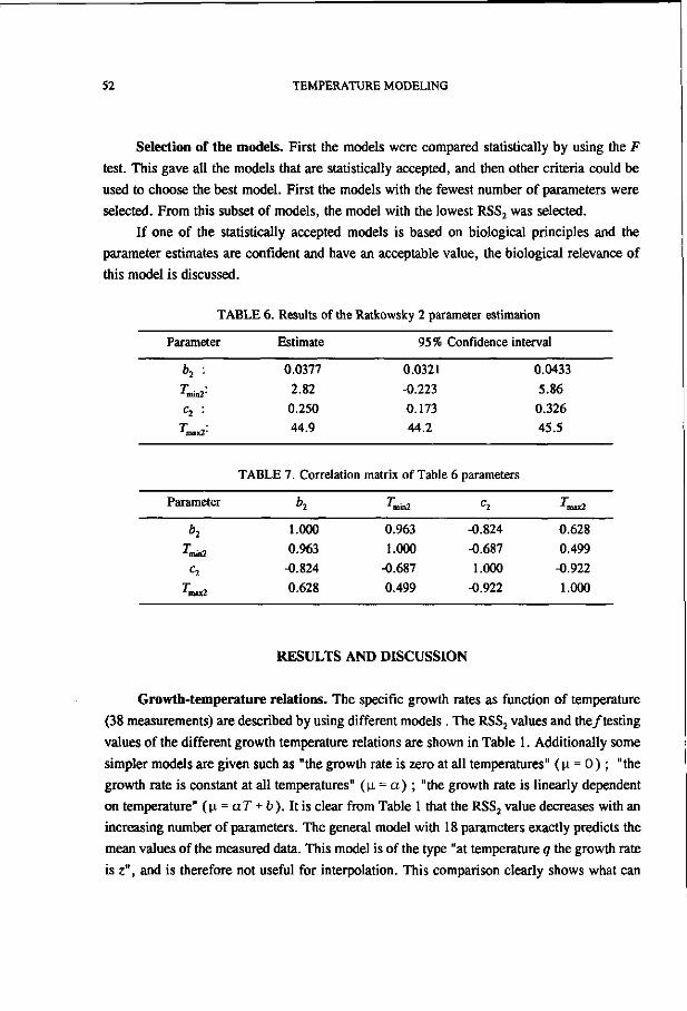
52 TEMPERATURE MODELING
Selection of the models. First the models were compared statistically by using the F
test. This gave all the models that are statistically accepted, and then other criteria could be
used to choose the best model. First the models with the fewest number of parameters were
selected. From this subset of models, the model with the lowest RSS2 was selected.
If one of the statistically accepted models is based on biological principles and the
parameter estimates are confident and have an acceptable value, the biological relevance of
this model is discussed.
TABLE 6. Results of the Ratkowsky 2 parameter estimation
Parameter
b2 : T
min2' c2 :
T nux2*
Estimate
0.0377
2.82
0.250
44.9
95 % Confidence interval
0.0321
-0.223
0.173
44.2
0.0433
5.86
0.326
45.5
TABLE 7. Correlation matrix of Table 6 parameters
Parameter
b2
T • min2 c2
^max2
b2
1.000
0.963
-0.824
0.628
T -*min2
0.963
1.000
-0.687
0.499
c2
-0.824
-0.687
1.000
-0.922
T
0.628
0.499
-0.922
1.000
RESULTS AND DISCUSSION
Growth-temperature relations. The specific growth rates as function of temperature
(38 measurements) are described by using different models . The RSS2 values and the/testing
values of the different growth temperature relations are shown in Table 1. Additionally some
simpler models are given such as "the growth rate is zero at all temperatures" ( [i = O ) ; "the
growth rate is constant at all temperatures" (\i = a) ; "the growth rate is linearly dependent
on temperature" (n = aT + ö). It is clear from Table 1 that the RSS2 value decreases with an
increasing number of parameters. The general model with 18 parameters exactly predicts the
mean values of the measured data. This model is of the type "at temperature q the growth rate
is z", and is therefore not useful for interpolation. This comparison clearly shows what can

CHAPTER 4 53
be achieved with modeling: reduction of data to a limited number of parameters, more
specifically to a model that is accepted statistically with as few parameters as possible. Some
investigators (1) only compare the RSS2 of models and decide which model is the best by
determining which model gives the lowest RSS2. From Table 1 it can be seen that there are
always models with a lower RSS2, even one with RSS2=RSS,. But these models have so many
parameters that the aim of modeling, reducing the data to a statistically accepted model with
a limited number of parameters, is not achieved. The lack of fit is probably a more stringent
test of model adequacy.
From the curvature of the datum points in Fig. 1, it can be easily seen that the data are
not well described by a constant value or a straight line. Indeed, for the first four models the
ƒ testing value is much larger than the F table value, and therefore these models are rejected.
From Table 1 it can be concluded that the Hinshelwood (four parameters), Ratkowsky 2 (four
parameters), Ratkowsky 3 (four parameters), and Schoolfield (six parameters) models are
accepted statistically, because the ƒ testing value is lower than the F value. In Fig. 1 to 4,
where for these four models the predicted and measured values are shown, it can be seen that
these models describe the curvature of the growth rate-temperature relation. As these four
models are all accepted statistically, other criteria can be used to choose the best model.
Among the four-parameter models, the Hinshelwood model is based on a fundamental
model (Arrhenius). In the Hinshelwood model, the parameters are strongly correlated (Table
3). A value of 1 for two parameters in the correlation matrix means that these two parameters
are totally correlated with each other. Parameters that are strongly correlated (> 0.999) are
difficult to estimate, because a change in one parameter will be compensated for by a change
in a correlated parameter, and numerous iterations are necessary. Moreover, the confidence
intervals of such parameters are very large (Table 2). A second problem with the
Hinshelwood model is that the estimates for the activation energies El and E2 are almost the
same value (107.2 and 107.4 kJ). This results in a subtraction of two large values to calculate
the growth rate. Reparameterization of the model, however, can possibly reduce these
problems. Normally, the activation energy for an enzyme-catalyzed reaction is 10 to 80 kJ,
and for a denaturation reaction it is 400 to 1200 kJ (3). Neither estimated activation energy
is within these intervals. This means that the fitting of the Hinshelwood relation to the data
results in an estimation of unrealistic activation energy values. This makes the biological
background of the model discussable. A third problem with the Hinshelwood model is that
the predictions of the growth rate at low temperatures are too high. Growth rates at low
temperatures are especially important during chilled food storage. Concluding all these
aspects, this model can be regarded as not appropriate.

54 TEMPERATURE MODELING
Temperature ( C)
FIG. 5. Asymptote data modeled with the Ratkowsky 4 model
( • : estimated asymptote values; : model prediction).
Ln(A) 8
10 20 30 40 50
Temperature ( C)
FIG. 6. Lag time data modeled with a hyperbola model
( • : estimated lag time values; : model prediction).

CHAPTER 4 55
Schoolfield et al. (13) reparameterized their model to overcome the correlation problem
and, as can be seen in Table 5, they were successful. The parameter Ht should be the enthalpy
of activation of the reaction that is catalyzed by the rate-controlling enzyme. A negative value,
however, was found. However, part of the confidence interval covers realistic values (Table
4). The other parameters also show realistic values. Therefore, the biological background of
the Schoolfield model can exist. However, often the six parameters of the Schoolfield model
are used as fitting parameters instead of estimates of biologically relevant parameters. Only
with a very large data set can this model be used to estimate the biological parameters. Even
with 38 datum points, the confidence intervals of the parameters are too large (Table 4).
As can be seen in Tables 7 and 9, the correlation matrices of the Ratkowsky 2 and
Ratkowsky 3 models show no nondiagonal values of > 0.999, so in these models the
parameters can be estimated easily.
TABLE 8. Results of the Ratkowsky 3 parameter estimation
Parameter
ft, : T
min3* c3 : T
max3*
Estimate
0.0410
3.99
0.161
43.7
95% Confidence interval
0.0335
0.881
0.0940
43.4
0.0485
7.11
0.228
44.1
TABLE 9. Correlation matrix for Table 8 parameters
Parameter
*3
T min3 c3
T max3
b3
1.000
0.960
-0.910
0.591
T 'mm3
0.960
1.000
-0.783
0.466
C3
-0.910
-0.783
1.000
-0.804
T 'max3
0.591
0.466
-0.804
1.000
Statistical evaluation of the models shows that the Hinshelwood, Ratkowsky 2,
Ratkowsky 3, and Schoolfield models all describe the growth rate data sufficiently.
Therefore, an appropriate model can be chosen on the basis of other grounds. The models
with the lowest number of parameters (the four-parameter models) were chosen. The
Ratkowsky 3 equation has the lowest RSS2 of all four-parameter models. Therefore, the

56 TEMPERATURE MODELING
Ratkowsky 3 model appeared to be the most suitable to describe the specific growth rate as
function of temperature. The RSS2 of the Ratkowsky 3 model is even smaller than the RSS2
of the Schoolfield model, although the Schoolfield model has two more parameters.
The Ratkowsky 3 equation shows an exponential drop of the growth rate at high
temperatures and it shows no positive values of the growth rate at temperatures above the
maximum growth temperature.
TABLE 10. Comparison of the models describing the asymptote
Model'
.4 = 0
A = a
A = aT
A-aT+b
Hinshelwood
Ratkowsky 2
Ratkowsky 3
Ratkowsky 4
Schoolfield
General
A-A{i.n
No. of
parameters
0
1
1
2
4
4
4
3
6
18
38
DF
38
37
37
36
34
34
34
35
32
20(DF,)
0
RSS2
2378
128
587
111
178
28.7
28.3
31.3
20.4
14.3(RSS,)
0.0
ƒ
183
9.37
47.1
8.41
16.4
1.43
1.39
1.58 0.711
F
2.1
2.2
2.2
2.2
2.2
2.2
2.2
2.2
2.3
* A is the asymptote to be modeled; A(i,j~) is they* asymptote at 7V a and b are regression coefficients; Tis the temperature. Bold indicates successive selection of the models.
Asymptote-temperature relations. The asymptote value as a function of temperature
was analyzed with various models (Table 10). The asymptote data did not differ much in the
lower temperature range, and therefore a model with a constant asymptote in the lower
temperature range was also taken into account (Ratkowsky 4). The first four models can be
rejected on basis of the F test. In this case, the Hinshelwood model is rejected also. None of
the other models can be rejected on the basis of statistics. While the Ratkowsky 4 model is
not rejected, there is no statistical evidence that there is an effect of temperature on the
asymptote in the lower temperature range. Although it seems that the asymptote value
increases with increasing temperature (Fig. 5), the measuring error is too large to
discriminate statistically. It is possible that with more datum points or data with a smaller
standard deviation the effect of temperature on the asymptote in the lower temperature range
can be shown. Yet, since for the measured datum points the Ratkowsky 4 model was accepted

CHAPTER 4 57
statistically and had the lowest number of parameters (from the models which are accepted),
this model was selected (Fig. 5). The parameter estimates of this model are shown in Table
11.
In these experiments, the same inoculation level (5 105 organisms per ml) was always
used. If it is assumed that the final absolute number of organisms JV_ is constant (and
therefore not dependent on the inoculum level), the asymptote is dependent on the inoculum
level as:
b 4 = / l = l n ( N . / W 0 ) (15)
ln(A/.) = b 4 + l nN 0 = 8.46 + ln(5£'5) = 8.46+ 13.12 = 21.58 (16)
The parameter bA (the final level reached at lower temperatures) must be used
[b 4+ln(5£"5)- ln( /V„) = 2 1 . 5 8 - ln(/V„)] if another inoculation level is used.
TABLE 11. Results of the Ratkowsky 4 parameter estimation
Parameter Estimate 95 % Confidence interval
K Q
T max4
8.46
1.25
43.1
8.09
0.709
42.9
8.82
1.78
43.4
Lagtime-temperature relation. To fit the lag time, a logarithmic transformation was
used, because the data showed a larger measuring error at high numerical values (the standard
deviation was proportional to the mean value). After the transformation, the distribution of
measuring errors at different temperatures was almost the same. Adair et al. (1) fitted the
logarithm of the inverse lag time data with the Schoolfield model and the square root of the
inverse of the lag time data with the Ratkowsky model. After transforming the model
predictions back to lag times, they calculated the RSS2 between their measured data and the
model predictions and they found, for instance, RSSRat= 16186 and RSS^^, = 683. If they
would have fitted the logarithm of the lag time data with the logarithm of the inverse of the
Ratkowsky model (as it is proposed in this report; equation 10) and transformed back to lag
time, they would have found RSSRat= 632. Note that the fitting to the models is done with
different models but that the calculation of the RSS values is done comparing lag time data
(without transformation) with model data. This is a striking example to show the importance
of the choice of the transformation before fitting.

58 TEMPERATURE MODELING
The logarithm of the lag time as a function of temperature was described with different
models (Table 12). In this case, the first four models were rejected again. All other models
were accepted. The models with the lowest number of parameters had to be selected. These
were the models with two parameters that are accepted statistically (Ratkowsky 1 and a
hyperbola). Between these latter two models, the hyperbola model had the lowest RSS2, and
therefore this model was selected (Fig. 6). The parameter estimates are given in Table 13.
TABLE 12. Comparison of the models describing the lag time
Model'
l n (K) -0
l n ( \ ) = a lnO) = a r
l n (X) -aT + b
Hyperbola (Ratkowsky 1) '
(Ratkowsky 2)->
(Ratkowsky 3)1
General
l n ( M - l n [ X . ( i . ; ) ]
No. of
parameters
0
1
1
2
2
2
4
4
18
38
DF
38
37
37
36
36
36
34
34
20(DF,)
0
RSS2
127
58.6
95.6
29.1
9.70
18.3
9.14
9.21
7.70(RSS!)
0.0
ƒ
17.2
7.79
13.4
3.47
0.325 1.71
0.267
0.282
F
2.1
2.2
2.2
2.2
2.2
2.2
2.2
2.2
" \ is the lag time to be modeled; \(<. J) is they* lag time at 7]; a and b are regression coefficients; Tis the temperature. Bold indicates successive selection of the models.
TABLE 13.
Parameter
P •
q •
Results hyperbolic
Estimate
23.9
2.28
parameter estimation
95% Confidence interval
19.1 28.7
1.19 3.37

CHAPTER 4 59
Growth curve-temperature relation. The different models can now be integrated.
Using equation 4, equation 9, and equation 11 and the estimated parameters for these models
(Table 14), the growth rate, asymptote, and lag time at every desired temperature can be
calculated, and using equation 1, a growth curve at that temperature can be described.
If the measured growth data are compared with the model predictions, the resulting
model can be evaluated (Fig. 7 to 10). The model describes the data adequately. The growth
rate at 6°C and the asymptote at 8.5°C are not very well estimated. The measured growth
rate at 6°C is a very small value (0.0164 h1) and is estimated by the model as 0.00675 h1.
The lag time at 6°C is estimated well, which results in a reasonable prediction of the dynamic
behavior over a long period (almost 3 months). The asymptote at 8.5°C is not very well
estimated. The reason can be found in the fact that the model prediction at 8.5°C in Fig. 5 is
greater than the datum points. All the other predictions (also at the temperatures not presented
here) agreed very well with the measured values. The model prediction is usually in between
the duplicate or triplicate observations.
TABLE 14. Parameters for models (equation 4), (equation 9) and (equation 11)"
Growth rate (M
[b3(T-Tmln3)f
Parameter
*3
T mio3
c3
T max3
m) (equation 4)
( l - e x p [ c 3 ( 7 - T ,
Estimate
0.0410
3.99
0.161
43.7
nax3)\}
Asymptote b 4 { l - e x p [
Parameter
*4
C* T
max4
(A) (equation 9) c,(T-Tmax4)]}
Estimate
8.46
1.25
43.1
Lag time (K) (equation 11)
l n ( K ) ' ( T - q )
Parameter Estimate
p : 23.9
q : 2.28
y = Aexpi-exp Vn- e
( \ - 0 + l (1)
For the parameter bt, 21.58-ln(/v„) must be used if another inoculation level is used.

60 TEMPERATURE MODELING
\n{N/No) 1 0
8
6
4
2
o'
-2
•
A i^A
* 8.5 C
D.'
S •-•*#.• ̂ - r
A A . • •
•
* ' /^ Vao°c
y/%
••
i i i i
500 1000 1500 2000 2500 time (h)
FIG. 7. Growth data and total model at 6.0 (solid symbols) and 8.5°C (open symbols).
Different symbols indicate different duplicates.
\n(N/No) 10
8
6
4
2
oo D D
o--
S /
/25.0°C / <*' / '
o.' /
9 7 • m / •
- =0 / °" /
'°*y &lm • ,
B ^ . "
/ ^ • #
/ • 15.1°C
I
•
• •
i
•
20 40 60 80 100
time (h)
FIG. 8. Growth data and total model at 15.1 (solid symbols) and 25.0°C (open symbols).
Different symbols indicate different duplicates.

CHAPTER 4 61
\n(N/No) 10
8
6
4
2
0
J 35.1°C Xf. i / * ^
£ *rVi8.2°c * 7 * /
S&2
* * * • "
*
•
i i i
20 40 60 80
time (h)
FIG. 9. Growth data and total model at 18.2 (solid symbols) and 35.1°C (open symbols).
Different symbols indicate different duplicates.
ln(/V/A/o) 8
6
4
2
0
-2
A - - * ' A- '
j,41.5°C
cuwTr
0
42.8°C
I I I I
10 20 30 40 50 time (h)
FIG. 10. Growth data and total model at 41.5 (open symbols) and 42.8°C (solid symbols).
Different symbols indicate different duplicates.

62 TEMPERATURE MODELING
Conclusions. We now have a model describing the growth curve of L. plantarwn in
MRS medium including lag time, growth rate, and asymptotic value. In these studies, a
simple medium was chosen to collect a large number of datum points as it was the objective
of this study to distinguish between models. With the model proposed here, growth over the
whole relevant temperature range can be predicted. In practical situations other media will be
used and the parameter values will have to be determined for that situation. Often a much
smaller number of datum points will be collected. This indicates again the importance of a
small number of parameters, because the solutions are more stable and the estimates of the
parameters have a larger number of degrees of freedom using a model with a smaller number
of parameters. In our case (38 experiments, 18 temperatures), models with a small number
of parameters are selected. But normally growth rates are measured at far less different
temperatures, so models with more parameters will not be relevant. Since the models are not
rejected with a large amount of data (38 growth curves at 18 different temperatures), it is not
advisable to use models with a larger number of parameters with many fewer datum points.
ACKNOWLEDGMENTS
This work was partly funded by Unilever Research Laboratory Vlaardingen. We wish to thank P.M. Klapwijk, J.P.P.M. Smelt, and H.G.A.M. Cuppers for valuable discussions and H.H. Beeftink and F.M. Rombouts for reading the manuscript.
REFERENCES
1. Adair, C , D.C. Kilsby, and P.T. Whittall. 1989. Comparison of the Schoolfield (non-linear Arrhenius) model and the square root model for predicting bacterial growth in foods. Food Microbiol. 6:7-18.
2. Arrhenius, S. 1889. Über die Reaktionsgeschwindigkeit bei der Inversion von Rohrzucker durch Säuren. Z. Phys. Chem. 4:226-248.
3. Christophersen, J. 1973. Basic aspects of temperature action on microorganisms, p. 3-59. In H. Precht, J. Christophersen, H. Hensel, and W. Larcher (ed.), Temperature and life. Springer-Verlag KG, Berlin.
4. Einarsson, H., and S.G. Eriksson. 1986. Microbial growth models for prediction of shelf life of chilled meat, p. 397-402. In Recent advances and developments in the refrigeration of meat by chilling. Institut International du Froid-International Institute of Refrigeration, Paris.

CHAPTER 4 63
5. Gill, C O . , D.M. Phillips, and M.P.F. Loef f en. 1988. A computer program for assessing the
remaining storage life of chilled red meats from product temperature histories, p. 73-77. In
Refrigeration for food and people. Institut International du Froid-International Institute of
Refrigeration, Paris.
6. Gompertz, B. 1825. On the nature of the function expressive of the law of human mortality,
and on a new mode of determining the value of life contingencies. Philos. Trans. R. Soc.
London 115:513-585.
7. Hinshelwood, C.N. 1946. Influence of temperature on the growth of bacteria, p. 254-257. In
The chemical kinetics of the bacterial cell. Clarendon Press, Oxford.
8. OIley, J., and D.A. Ratkowsky. 1973. Temperature function integration and its importance in
the storage and distribution of flesh foods above the freezing point. Food Technol. Aust.
25:66-73.
9. Phillips, J.D., and M.W. Griffiths. 1987. The relation between temperature and growth of
bacteria in dairy products. Food Microbiol. 4:173-185.
10. Ratkowsky, D.A., R.K. Lowry, T.A. McMeekin, A.N. Stokes, and R.E. Chandler. 1983.
Model for bacterial culture growth rate throughout the entire biokinetic temperature range. J.
Bacteriol. 154:1222-1226.
11. Ratkowsky, D.A., J. OIley, T.A. McMeekin, and A. Ball. 1982. Relationship between
temperature and growth rate of bacterial cultures. J. Bacteriol. 149:1-5.
12. Schnute, J. 1981. A versatile growth model with statistically stable parameters. Can. J. Fish.
Aquat. Sei. 38:1128-1140.
13. Schoolfield, R.M., P.J.H. Sharpe, and C.E. Magnuson. 1981. Non linear regression of
biological temperature-dependent rate models based on absolute reaction-rate theory. J. Theor.
Biol. 88:719-731.
14. Sharpe, P.J.H., G.L. Curry, D.W. DeMichele, and C.L. Cole. 1977. Distribution model of
organism development times. I. Theor. Biol. 66:21-38.
15. Sharpe, P.J.H., and D.W. DeMichele. 1977. Reaction kinetics of poikilothermdevelopment.
J. Theor. Biol. 64:649-670.
16. Spencer, R., and C.R. Baines. 1964. The effect of temperature on the spoilage of wet white
fish. Food Technol. 5:175-181.
17. Stannard, C.J., A.P. Williams, and P.A. Gibbs. 1985. Temperature/growth relationship for
psychrotrophic food-spoilage bacteria. Food Microbiol. 2:115-122.
18. Zwietering, M.H., I . Jongenburger, F.M. Rombouts, and K. van 't Riet. 1990. Modeling
of the bacterial growth curve. Appl. Environ. Microbiol. 56:1875-1881. Chapter 2 of this
thesis.

CHAPTERS
EVALUATION OF DATA TRANSFORMATIONS AND VALIDATION OF MODELS FOR THE EFFECT OF TEMPERATURE ON
BACTERIAL GROWTH
ABSTRACT
The temperature of chilled foods is an important variable for controlling microbial
growth in a production and distribution chain. Therefore, it is essential to model growth as a
function of temperature in order to predict the number of organisms as a function of
temperature and time. This paper deals with the correct variance-stabilising transformation of
the growth parameters A,\i, and X. This is of eminent importance for the regression
analysis of the data. A previously gathered data set is extended with new data. With the total
data set (original and new data), an analysis of variance is carried out to determine which
transformation should precede fitting. For the asymptote data no, for the growth rate a square
root, and for the lag time a logarithmic transformation was found to be appropriate. Model
corrections were made and model parameters were estimated using the original data. The
models were validated with the new data. The predictions of the models for \i and A, were
adequate. The model for A showed a significant deviation, therefore a new model for A is
proposed. Finally, the model parameters were updated using the total data set.
INTRODUCTION
Temperature is a major factor determining the progress of many food deterioration
reactions. For microbial spoilage the effect of temperature on the specific growth rate and the
lag phase is important. Various models to describe the effect of temperature are used (7).
Models often are compared only to the data on which the model is fitted (measured versus
This chapter is submitted as:
Evaluation of Data Transformations and Validation of Models for the Effect of Temperature on
Bacterial Growth
M.H. Zwietering, H.G.A.M. Cuppers, J.C. de Wit, K. van 't Riet

66 MODEL VALIDATION
fitted) and are only rarely validated with new data (measured versus predicted). Yet, such
validation can provide useful information about the accuracy and predicting value of the
models.
The effect of temperature on growth rate is modeled often after a transformation (square
root or logarithm). This transformation, however, changes the distribution of errors.
Unweighted regression may only be performed if the variance is equally distributed with
temperature. Therefore, it is of great importance to determine which type of transformation
gives a temperature-independent variance. Ratkowsky (3) used multiple measurements at each
temperature to calculate the variance. He advises to use a square-root transformation to
stabilize variance for the growth rate [or (generation time)05] and a logarithm for the lag
phase duration. Alber and Schaffner (1) used the in-experiment error (no replicates) to
calculate the variance and recommended to use a logarithmic transformation to stabilize the
variance of the growth rate. In our former paper (7) the growth rate and the asymptote were
modeled without transformation since the variance seemed to be equally distributed in that
particular data set. The lag time was fitted after a logarithmic transformation, since this
transformation smoothed the variance.
It will be clear that different opinions do exist up till now. This is largely due to the
rather small data sets that were used. In order to estimate the variance at least duplicate
measurements at each temperature are needed. With an extensive data set it can be examined
with which transformation the variance is stable over a large temperature interval.
THEORY
Description of the experimental bacterial growth rate data. Growth curves are
defined as the logarithm of the relative population size [ ln(jV/A/„)]asa function of time.
A sigmoidal growth model (modified Gompertz) with three parameters can describe the
growth curve (6), at a given temperature.
ln(A///V„) = y4exp< - e x p - ( \ - 0 + 1 (1)
with A = Asymptotic level ln(A/„/A/0), n m = maximum specific growth rate (h1),
X = lag phase duration (h), and e = exp(l).

CHAPTER 5 67
Analysis of Variance. The variances of A,\im, and A. are calculated at different
temperatures using the mean values of the measured data. At one temperature Tit mi replicate
curves are measured. In our case, m, does not have the same value at different temperatures.
Then the model for the best prediction of the y-value ( A, \i, or X. ) at a certain temperature
can be proposed, that is defined as the mean value y(Q of the measured y-values at that
temperature. This model is called the general model:
with y = A,[i, or X; y ( i, ;' ) being they*y-valueat Tt, and y ( i ) being the mean y-value
atr. The variance at temperature T, is calculated at those temperatures for which more than
one observation is obtained with:
R s s ( = £ [ y ( i . y ) - y ( 0 ] 2
2 RSS; (3) s, = DF<
with RSSj the Residual Sum of Squares at 7]; DF; the Degrees of Freedom at 7j (equals m-\);
and s f the residual variance at Tt.
According to Ratkowsky (3) the variance can be plotted against the mean value, as well
as the variance divided by the mean, the square of the mean, and the cube of the mean, in
order to determine the appropriate transformation. If the variance is dependent on the mean,
models should be fitted after transforming the data or by using non-normal error assumptions.
If the variance divided by the mean shows no correlation a square root transformation is
suitable [ v a r (yy j ) = v a r ( y j ) / 4 y ( ] . If the variance divided by the square of the mean
shows no correlation a logarithmic transformation is suitable to correct for heterogeneity of
variance [ v a r ( l n [y , ] ) = v a r ( y ( ) / y f ] .
As an alternative procedure the variance is calculated after carrying out the
transformation (the variance of the transformed data). Then the variance of the untransformed
data, the square root and the logarithm of the data are plotted against the mean.

68 MODEL VALIDATION
To quantify correlation (for both above mentioned methods) linear regression is carried
out and the correlation coefficient is calculated. With a t test it can be examined if there is a
correlation
-'M with t =Mesting value; r = correlation coefficient; n = number of observations.
It should be noted that linear regression is used, although the relations will not be linear.
This gives a global indication of the correlation and not an exact value. Visual inspection of
the variance data is also crucial.
Growth/temperature relations. The previously proposed models for the effect of
temperature on the asymptote (A), specific growth rate (M-m), and lag time (A.) with
parameter values are given in Table 1.
TABLE 1. Parameter values and models for the effect of temperature on the asymptote (A), growth rate (tim) and lag time (\) for Lactobacillusplantarum in MRS-medium
[from Zwietering et al. (7)]
Asymptote, Ratkowsky 4 bA 8.46" ^ = b 4 { i - e x p [ c 4 ( r - r m o x < ) ] >
Specific growth rate, Ratkowsky 3
Hm = [b3(7--7"m ,„ 3 ) ] z<l-exp[c 3 (7 ' -7- 1 ) u , x 3 ) ]}
Lag time, hyperbola
P ln(M =
c4
T max4
b3
T mtn3
c3
T max3
P
a
1.25
43.1
0.0410
3.99
0.161
43.7
23.9
2.28 (T-q)
' Parameter bA depends on the inoculation level according to the equation ft4=21.58-ln(A/0).
The hyperbolic model for the lag time has the complication that the lag time at higher
temperature approaches asymptotically to one (the logarithm of the lag time approaches zero).
This is of course an arbitrary value, and it is independent of the unit in which the lag time is
expressed. This is an undesirable imperfection of the hyperbolic model. Furthermore, it can

CHAPTER 5 69
be assumed that the lag phase increases at temperatures higher than optimum, which can also
be seen in the data. The hyperbolic model, however, does not show such behaviour.
Therefore, the previously proposed reciprocal of the Ratkowsky model (equation 5) is
reconsidered, since this model overcomes these two problems. However, this model contains
four parameters. This can be overcome by assuming Tmja and Tnax values, and eventually also
the c value to be equal to the parameters of the equation describing the growth rate.
l n ( \ ) = ln 2
b s (T -T m l „ 5 ) - { l - e x p [ c 5 ( T - T m Q x 5 ) ] } ' (5)
Comparison of the models. The models are validated statistically with the use of the F
ratio test. With the general model (equation 2), the measuring error is estimated by
determining the deviation of the measured values from the mean value at one temperature.
The sum of squares of the deviations between the data and the general model is calculated for
all temperatures (RSSg):
k k
RSS5= ^ RSS ;= ^ ^ [ y ( i , y ) - y ( 0 ] 2 (general model) (6) i - l i - l / - l
with y ( i, j ) being the7th y-value at T-t and y ( O being the mean v-value at T{.
The sum of squares of the deviations between the data and the given growth temperature
model (RSSJ is calculated as:
* mi
RSSm= Y. X [ y ( ' - - / ) ~ y ( 0 ] 2 ( g rowth - t empe ra tu r e model) (7) i - l y ' - l
with y ( O being the model prediction at temperature Tr
RSSm will always be larger than RSSg. The RSSm of the growth-temperature model
consists of both the measuring error and the lack of fit; therefore, the difference between the
RSSm of the model and the RSSg (the SS due to the measuring error) is calculated as an
estimate of the lack of fit. If the mean square of the lack of fit [(RSSm-RSSg)/(DFm-DFg)] is
of the same order of magnitude as the mean square of the measuring error (MScrror), the model
is adequate. This comparison between the lack of fit and the measuring error can be quantified
statistically by the ƒ testing value:

70 MODEL VALIDATION
(RSS m -RSS g ) / (DF m -DF g ) . - " . - D F ,
ƒ * TT^ tested aga ins t FDF" r i r ' (8)
where DFg is the number of degrees of freedom due to the residual variance, that equals the
total number of observations minus the number of different temperatures at which is
measured; DFm is the number of the degrees of freedom from the growth-temperature model
that equals the number of observations minus the number of parameters. MSerror= the mean
square of the measuring error with DFcrror degrees of freedom.
MATERIALS AND METHODS
Microbial experiments. In 60 experiments at 17 different temperatures, Lactobacillus
plantarum (American Type Culture Collection determined; no ATCC number) was cultivated
in MRS medium (Difco Laboratories). The culture was stored frozen (-16°C). The bacteria
were cultivated twice at 30°C, for 24 h and for 16 h. Growth was monitored in 20 ml tubes,
each containing 10 ml of medium and inoculated with the test organism to reach a target initial
titer of 5 105 CFU/ml. The test tubes were incubated statically at different temperatures from
6°C up to 40°C as follows (temperatures in °C and number of experiments in parentheses):
6.0 (1); 8.9 (1); 9.8 (7); 10.0 (5); 11.9 (1); 14.0 (1); 14.9 (6); 15.2 (5); 16.7 (3); 18.2 (1);
19.8 (6); 20.2 (7); 24.8 (7); 25.0 (6); 30.0 (1); 34.9 (1); 40.8 (1). At appropriate time
intervals (depending on temperature), the inoculated cultures were vortexed and samples of
0.1 ml were removed for serial dilution in peptone saline solution (1 g of Bacto-Peptone
[Difco], 8.5 g of NaCl [Merckp.a.] per liter). Bacterial numbers were determined with apour
plate (MRS medium with 12 g of agar [Agar Technical Oxoid Ltd.] per liter). The pour plates
were incubated for 48 h at 30°C before counting.
Fitting of the data. The model equations were fitted to the data by nonlinear regression.
RESULTS AND DISCUSSION
Analysis of variance. The previously measured data set [38 growth curves, from
Zwietering et al. (7)] was extended with new data (60 growth curves). From this total data
set (98 growth curves) only the sub-set of growth parameters up to 35 °C (80 growth curves,
at 17 different temperatures) was used to determine the variance at different temperatures.
This sub-set is used since above the optimum temperature (35°C) the variances are much

CHAPTER 5 71
larger than below the optimum, since the growth decreases rapidly, resulting in large errors.
With this sub-set the variance is analysed to find which transformation: none, a square root
one, or a logarithmic one (In), is necessary. The variance at different temperatures as function
of the mean value of the variable is given in Fig. 1,2, and 3. Furthermore, the variance
divided by the mean, divided by the square of the mean, and divided by the cube of the mean
are given. For these data the correlation coefficient was determined by performing a linear
regression of the variance data. With the t test it was determined if correlation was significant.
The results are given in Table 2.
Additionally, the data are transformed (with a square-root, a logarithmic, and a
reciprocal root transformation) and the variances of the transformed data are calculated. Also
with these data a linear regression is performed. These regression data with t testing value as
well are given in Table 2.
TABLE 2. Results of determination of the correlation coefficient by performing a linear regression of the variance data as function of the mean of the data
A
var
var/mean
var/mean2
var/mean3
H
var
var/mean
var/mean2
var/mean3
\
var
var/mean
var/mean2
var/mean3
r'
0.0305
-0.00440
-0.0442
-0.0900
r*
0.671
0.0375
-0.357
-0.299
r'
0.998
0.978
0.146
-0.238
t value b
0.118 -0.0171
-0.171
-0.350
t value b
3.51
0.145
-1.48 -1.22
t value b
60.9
18.1
0.573
-0.949
Transformation
A
u l n ( / l )
\/(A
Transformation
P-
4Ï>-In(n)
1/V^i
Transformation
X
fr ln(M
1 / ^
r'
0.0305
-0.0178
-0.0686
0.123
r"
0.672
0.0176
-0.671
0.848
r'
0.998
0.975
0.331
0.321
t valueb
0.118
-0.0689 -0.266
0.478
t valueb
3.51
0.0681
-3.51
6.19
t value b
60.9
17.0
1.36 1.31
" correlation coefficient. b The 95% critical t value for 15 degrees of freedom is 2.13. Bold values indicate no significant correlation.

72 MODEL VALIDATION
var(>A)
3-
2-
1 :
n-D
D D
a
D
a a
— i — i — 1 — 1 — F ™ " ! — i -
a
var(>A)/(mean/\) 0.4
var(A)/(meanA)'
meanA
FIG. 1. Variance of A, variance divided by the mean and divided by the square
of the mean, plotted against the mean of A.

CHAPTER 5 73
var(/i) 0.006
0.004-
0.002
var(jH)/(mean^i) 0.006
var(^)/(meanjU)'
i 0.2 0.4 0.6 0.8 1 1.2 mean jl
FIG. 2. Variance of n , variance divided by the mean and divided by the square
of the mean, plotted against the mean of \i.

74 MODEL VALIDATION
varQ)/(mean )) 150
100-
50
Q | » o , Qo—oJ | a Po D—
var())/(mean )) 1
0.8
0.6-
0.4-
0.2
0 O D
° n " , " 0_
varQ)/(mean \) 0.06
0.04- D
0.02
_n ,-Q B_
In (mean ) ) FIG. 3. Variance of X. divided by the mean and divided by the square and
the cube of the mean, plotted against logarithm of the mean of \ .

CHAPTER 5 75
Fig. 1 shows that the variance of the asymptote gives no clear correlation with the mean.
This holds also for the variance divided by the mean, divided by the square of the mean, and
divided by the cube of the mean. In Table 2 it can be seen that with both methods for all cases
no significant correlation is found. Therefore, it can be concluded that transformations do not
stabilize the variance and no transformation should be used for the asymptote data.
In Fig. 2 it can be seen that the variance of the growth rate shows a positive correlation
with the mean. The variance divided by the mean shows no clear correlation, and the variance
divided by the square of the mean shows a negative correlation. In Table 2 it can be seen that
the variance of the growth rate gives a significant correlation with the mean. The variance
divided by the mean, the variance divided by the square of the mean, and divided by the cube
of the mean, show no significant correlation. If the growth rate data are transformed all cases
give a significant correlation, except for the square root transformation. Therefore, the square
root transformation is chosen to stabilize the variance of the growth rate data.
In Fig. 3 it can be seen that the variance of the lag time divided by the mean shows a
positive correlation with the logarithm of the mean (because of the large range of lag-time
values a logarithmic transformation is used in these graphs). The variance divided by the
square of the mean shows no, and the variance divided by cube of the mean, shows a negative
correlation. In Table 2 it can be seen that the variance, and the variance divided by the mean
show a significant correlation. If the lag time data are transformed, no transformation and a
square root transformation give a significant correlation. The logarithm and reciprocal root
transformation give no significant correlation. Concluding, the logarithmic transformation is
chosen to stabilize the variance of the lag time data.
TABLE 3. Results of the Ratkowsky parameter estimation for the 4\i data
Parameter Estimate 95% Confidence interval
7* min2
0.0385 3.37 0.256 44.7
0.0343 to 0.0427
1.60 to 5.13 0.175 to 0.336 44.1 to 45.4
• / M ^ - b 2 (T -T m , „ 2 ) ( 1 - e x p [ c 2 ( T - T„ 2 ) ] >
No. of parameters DF RSS MS ƒ
Ratkowsky LOF
General 18
34 14 20
0.125 0.023 0.102
0.00367 0.00162 0.00511
0.317 2.2
LOF= Lack of Fit; DF= Degrees of Freedom; RSS= Residual Sum of Squares; MS= Mean Square; ƒ= MSLOF/MSgeneral; F= F table value (95% confidence).

76 MODEL VALIDATION
Model update. Now that with the analysis of variance the correct transformations are
found, the previously proposed models (7) can be updated. For the asymptote no
transformation was used in our former model development and the analysis of variance shows'
that transformation is not necessary, therefore the model and model parameters determined
from the original data set remain unchanged. As shown by the analysis of variance the square
root transformation is the best transformation to stabilize the variance of the growth rate data.
Therefore, the model should be fitted to the square root of the data. The results of fitting the
previously measured data (7) to the square root relation are given in Table 3. The lack of fit
of the model is compared to the measuring error and the square root relation is accepted on
basis of the F test.
(-)
10
, * c a J" ° ° in»0
D w X|
8 O OD°
0.2 0.4 0.6 0.8 1
FIG. 4. Product of n*X against n .
1.2
// (h )
For the lag time data the logarithmic transformation is stabilizing the variance, and was
already used (7). However, the previously proposed reciprocal of the Ratkowsky model
(equation 5) is also tested. If it is assumed that the Tmin and 7max value are equal to the Tmin and
Tma value of the equation describing the growth rate, this model also contains two parameters.
If also the c-value is fixed, the model contains only one parameter. The results of fitting the
previously measured lag time data to the hyperbolic model and reciprocal square root relation
are given in Table 4. The reciprocal Ratkowsky model with all parameters fixed, except for
b is accepted by the F test. This result indicates that the lag time is reciprocally proportional

CHAPTER 5 77
TABLE 4. Results of the reciprocal Ratkowsky parameter
Parameter
P
q
Estimate
23.9
2.28
95% Confidence
interval
19.1 to 28.7
1.19 to 3.37 ln(M-
P (T-
estimation for the in(k) data
<7) model 1
0.0274 0.0240 to 0.0308 3.37 fixed 0.373 0.228 to 0.518 44.7 fixed
ln(\) = -21n| «>s (7--3.37X1 -exp[c s(r-44.7)]} I
model 2
h T
min5
C5 T max5
Model 1
LOF 1
Model 2
LOF 2
Model 3
LOF 3
General
0.0299
3.37
0.256
44.7
0.0268 to 0.0329
fixed
fixed
fixed
No. of parameters
2
2
1
18
ln(M =
DF
36
16
36
16
37
17
20
-21nfb s (T
RSS
9.70
2.00
12.65
4.95
14.03
6.33
7.70
-3.37){1 -exp[0.256(7-
model 3
MS
0.269
0.125
0.351
0.309
0.379
0.372
0.385
ƒ
0.325
0.803
0.967
-44.7)]})
F
2.2
2.2
2.2
LOF= Lack of Fit; DF= Degrees of Freedom; RSS= Residual Sum of Squares; MS= Mean Square; ƒ= MSL0F/MSgen<:ral; F= F table value (95% confidence).
to the growth rate. This was already suggested by Simpson et al. (4). Similar results for the
7"min value for the growth rate and lag time are also given by Chandler and McMeekin (2) and
Smith (5). The multiplication of the growth rate and lag time are given in Fig. 4. This graph
shows that the growth rate and the lag time are reciprocally proportional (except for one point)
over a large range of growth rate values. This model now contains only one parameter and
predicts a lag time increase at higher temperature.
The updated models and parameter values, based on the previously measured data (7)
are given in Table 5.

78 MODEL VALIDATION
TABLE 5. Parameter values and modeis for the effect of temperature on the asymptote (A ),
specific growth rate (nm) and lag time ( \ ) for Lactobacillusplantarwn in MRS-medium
Asymptote, Ratkowsky 4
j l - 6 , { l - e x p [ c , ( T - r m o r t ) ] ) \ 8.46
1.25
43.1
Specific growth rate, Ratkowsky
7 ( ^ = b 2 (7 ' -7 'm ,„ 2 ){l -exp[c 2 ( r - rm G x 2 ) ]}
0.0385
3.37
0.256
44.7
Lag time, reciprocal Ratkowsky
ln (*0--21n b5(7"-7"mM) < 1 - exp[c5(7- - T ma„m
0.0299
3.37
0.256
44.7
n°c) FIG. 5. New asymptote data and model ( ) based on previously measured data.

CHAPTER 5 79
FIG. 6. New growth rate data and model ( ) based on previously measured data.
In()) 8
6
4
2 -
n
\ a
5 ^v °m ^ | o J
-4c--o
9
a /
0 10 20 30 40
n°c) FIG. 7. New lag time data and reciprocal Ratkowsky model ( ) and hyperbolic model (-
based on previously measured data.

80 MODEL VALIDATION
Model Validation. Now the updated model can be used to predict the newly measured
data (60 growth curves, measured at 17 different temperatures). The newly measured growth
parameters are plotted with the predictions in Fig. 5, 6, and 7. The growth rate is transformed
with a square root, and the lag time is transformed with a logarithmic (In) transformation.
From these graphs it can be concluded that the data are reasonably well predicted by the
earlier developed models. For the growth rate data the residuals show no trend. However, the
lag-time data and the asymptote data show some discrepancies (the residuals are not equally
well distributed around zero). It should be noted that the new data are all at temperatures
below 40°C. Therefore, the models are only validated within the range 6-40°C. Furthermore,
it should be noted that the new data are compared with predictions using parameter values
determined with other data.
TABLE 6. Result of the F-test, comparing new data and model
Rsse i ror
DF error
MSOT0,
RSSg (DFg=
RSS n (DFm=
LOF (DF^p
MSL O F
ƒ
43)
=60)
= 17)
A
31.3
35
0.895
Ratkowsky 4
9.79
59.0
49.2
2.90
3.24
•JÏÜ
0.125
34
0.00367
Ratkowsky
0.0269
0.0425
0.0157
0.000921
0.251
l n ( M
14.0
37
0.379
Hyperbole
2.39
13.1
10.8
0.633
1.67
(Ratk)i
2.39
10.4
8.00
0.470
1.24 F£~2.00
RSS= Residual Sum of Squares; DF= Degrees of Freedom; MS= Mean Square; error= error previous data; RSSg= RSS of general model (mean of replicates); RSSm= RSS of model prediction; (Ratk)-^ reciprocal Ratkowsky model (equation 5); LOF= Lack Of Fit (RSSm-RSSg); ƒ= MSLOF/MSerror; F= F table value (95% confidence).
The lack of fit of the models is compared with the measuring error by the F-test (Table
6). The mean square of the lack of fit must be tested against the mean square of the measuring
error. The measuring error is estimated by calculating the deviation of the first set of data
with the growth model. The lack of fit is calculated by subtracting the RSS of the growth

CHAPTER 5 81
temperature model (RSSm with D F m = 6 0 - 0 = 6 0 ; the number of observations minus the
number of parameters) and the RSS due to the residual variance (RSSg with D F g = 6 0 - 1 7 = 4 3 ;
total number of observations minus the number of different temperatures measured).
F rom this statistical test we can conclude that for the growth rate data and the lag t ime
data the deviation between the model prediction and the data is of the same order as the
measuring error. The reciprocal Ratkowsky model had a better predicting ability (in this case)
than the hyperbola model .
Fo r the asymptote data, however, there is a significant deviation between the model and
the data (this can also be seen globally in F ig. 5) .
Parameter update . Now that the model is validated the parameters can b e updated
using all data together. So finally, the model parameters a re updated using all 98 growth
curves. The final model parameters are given in Table 7 . By comparing the parameters in
Table 7 (parameters based on 98 growth curves) and Table 5 (parameters based on 38 growth
curves) it can be seen that the update resulted in small changes only. The results a re shown
graphically in F ig . 8 to 10.
TABLE 7. Parameter values and models for the effect of temperature on the
asymptote (A), specific growth rate ( i im) and lag time (K) for
Lactobacillus plantarum in MRS-medium, final parameter values
Estimate 95% Confidence
interval
Asymptote, Ratkowsky 4
/ l - b 4 < l - e x p [ c 4 ( r - 7 - „ , „ „ ) ] }
8.83
1.05
43.2
8.63 to 9.02
0.679 to 1.43
42.9 to 43.4
Specific growth rate, Ratkowsky
/ iü-bz(7"-rm l t ó ){ l -exp[c3(T-7-m l I , 2 ) ]> T min2
0.0385
3.29
0.247
44.8
0.0368 to 0.0402
2.63 to 3.95
0.207 to 0.288
44.4 to 45.2
Lag time, reciprocal Ratkowsky
l n ( \ ) - - 2 1 n b 5 ( r - r m , „ 5 ) { l - e x p [ C 5 ( r - 7 m a x 5 ) ] >
b5 0.0276
Tmini 3.29 c5 0.247
7L.« 44.8
0.0263 to 0.0289

82 MODEL VALIDATION
FIG. 8. All asymptote data and updated model ( ). Solid blocks are outlayers.
v*
FIG. 9. All growth rate data and updated model ( ).

CHAPTER 5 83
Inrt)
FIG. 10. All lag time data and updated model ( ).
Asymptote model. It is shown that there is a significant deviation between the .nodel
and the asymptote data (Fig. 5, 8 and Table 6). Therefore, another model is attempted. The
following model is proposed:
A = a ( ' ' min6 ) ( ' ' max6 J
( T - b 6 ) ( r - c 6 ) (9)
In this model parameter b6 must be somewhat lower than rmin6 and c6 must be a little
higher than Tmx6 (b6 and c6 being the temperatures at which the asymptote will reach minus
infinity). The results of fitting this equation are given in Table 8. The datum points indicated
with a solid box in Fig. 8 are not taken into account, since these data deviate largely. The
rejection of three points out of 98 seems justified.
It can be seen in Table 8 that the Ratkowsky 4 model is rejected on basis of the F test
and the newly proposed model is accepted. The confidence interval of 7 ^ includes the 7"min
value of the growth rate data (Tables 7 and 8), so this value can be fixed. The confidence
interval of 7 ^ does not include the Tnax value of the growth rate data. With a fixed 7 ^ value
the model is also accepted by the F test and this model is shown graphically in Fig. 11. It
shows a decrease of the asymptote values (number of cells ultimately produced) at extremes
of temperatures. These effects may result from the relative increase of the maintenance
energy at low growth rates. If more energy is consumed for maintenance, a lower cell number

84 MODEL VALIDATION
FIG. 11. All asymptote data and new model (- -).
will be reached. The decline at low temperatures was mentioned in our previous paper (7),
but could not be proven statistically with 38 observations. With the current 95 observations
this effect is shown to be statistically significant.
CONCLUSIONS
It has been shown with 80 growth curves at 17 different temperatures, that the
asymptote can best be modeled without transformation, the growth rate with a square root
transformation, and the lag time with a logarithmic transformation. The choice of the
transformation is of eminent importance for the regression analysis of the data.
The previously proposed lag time model has the complication that the lag time at higher
temperatures approaches an arbitrary value of one, while at higher temperatures it can be
assumed that the lag phase increases. Therefore, the previously proposed reciprocal of the
Ratkowsky model (equation 5) seems better. For this reason, the hyperbolic model is replaced
by the reciprocal Ratkowsky model.
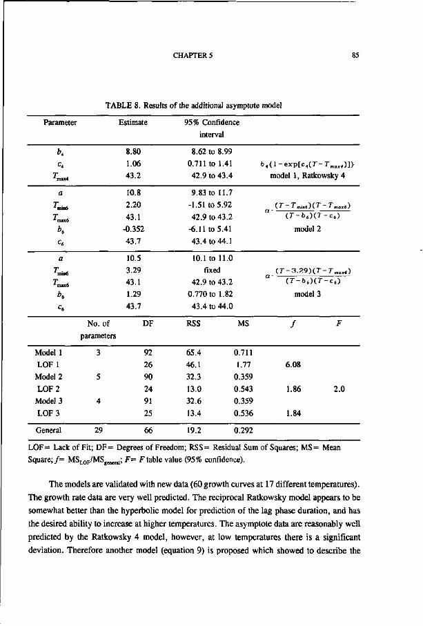
CHAPTER 5 85
TABLE 8. Results of the additional asymptote model
Parameter Estimate 95% Confidence interval
K c*
T nux4
a
T mm6
T max6 h c„ a
T min6 T
max6 b6
Ce,
8.80
1.06
43.2
10.8
2.20
43.1
-0.352
43.7
10.5
3.29
43.1
1.29
43.7
8.62 to 8.99
0.711 to 1.41
42.9 to 43.4
9.83 to 11.7
-1.51 to 5.92
42.9 to 43.2
-6.11 to 5.41
43.4 to 44.1
10.1 to 11.0
fixed
42.9 to 43.2
0.770 to 1.82
43.4 to 44.0
b 4{l-exp[c , (7-- : r „„ , ) ]}
model 1, Ratkowsky 4
(T - Tmin6^(.T ~ Tnax() a ( r - b 6 ) ( r - c 6 )
model 2
( r - 3 . 2 9 ) ( T - r m o » 5 ) a ( r - b 6 ) ( r - c 6 )
model 3
No. of parameters
DF RSS MS ƒ
Model 1
LOF 1
Model 2
LOF 2
Model 3
LOF 3
3
5
4
92
26
90
24
91
25
65.4
46.1
32.3
13.0
32.6
13.4
0.711
1.77
0.359
0.543
0.359
0.536
6.08
1.86
1.84
2.0
General 29 66 19.2 0.292
LOF= Lack of Fit; DF= Degrees of Freedom; RSS= Residual Sum of Squares; MS= Mean Square; ƒ= MSLOF/MSgcnerI1; F= F table value (95% confidence).
The models are validated with new data (60 growth curves at 17 different temperatures).
The growth rate data are very well predicted. The reciprocal Ratkowsky model appears to be
somewhat better than the hyperbolic model for prediction of the lag phase duration, and has
the desired ability to increase at higher temperatures. The asymptote data are reasonably well
predicted by the Ratkowsky 4 model, however, at low temperatures there is a significant
deviation. Therefore another model (equation 9) is proposed which showed to describe the

86 MODEL VALIDATION
behaviour at low temperatures much better. The decline at low temperatures could now be
proven statistically with the current 95 observations. For kinetic predictions the lag time and
the growth rate are the most important parameters.
ACKNOWLEDGMENTS
This work was partly funded by Unilever Research Laboratory Vlaardingen. The authors wish
to thank P.M. Klapwijk, P.F. ter Steeg, and J.P.P.M. Smelt for valuable discussions and H.H.
Beeftink for reading the manuscript. The authors wish to thank L.A. Ledelay, B.A. Campfens, and
E.W. Oosterom for carrying out most of the experiments.
REFERENCES
1. Alber, S.A., and D.W. Schaffner. 1992. Evaluation of data transformations used with the
square root and Schoolfield models for predicting bacterial growth rate. Appl. Environ.
Microbiol. 58:3337-3342.
2. Chandler, R.E., and T.A. McMeekin. 1985. Temperature function integration and its
relationship to the spoilage of pasteurized homogenized milk. Austr. J. Dairy Technol.
40:37-40.
3. Ratkowsky, D.A. 1992. Predicting response times in predictive food microbiology. Dept. of
Primary Industry, Fisheries and Energy, Tasmania, Research and Development Unit,
Biometrics Section, Occasional Paper No. 1992/1.
4. Simpson, R., K.Y. Li, and J.A. Torres. 1989. A management tool to improve the microbial
quality of refrigerated foods, p. 155-168. In Proceedings of an international conference on
technical innovations in freezing and refrigeration of fruits and vegetables, University of
California, Davis USA Publ. International Institute of Refrigeration.
5. Smith, M.G. 1985. The generation time, lag time, and minimum temperature of growth of
coliform organisms on meat, and the implication for codes of practice in abattoirs. J. Hyg.
Camb. 94:289-300.
6. Zwietering, M.H., I. Jongenburger, F.M. Rombouts, and K. van 't Riet. 1990. Modeling
of the bacterial growth curve. Appl. Environ. Microbiol. 56:1875-1881. Chapter 2 of this
thesis.
7. Zwietering, M.H., J.T. de Koos, B.E. Hasenack, J.C. de Wit, and K. van 't Riet. 1991.
Modeling of bacterial growth as function of temperature. Appl. Environ. Microbiol.
57:1094-1101. Chapter 4 of this thesis.

CHAPTER 6
MODELING OF BACTERIAL GROWTH WITH SHIFTS IN TEMPERATURE
ABSTRACT
The temperature of chilled foods is an important variable for the shelf life of a product
in a production and distribution chain. To predict the number of organisms as a function of
temperature and time, it is essential to model the growth as a function of temperature. The
temperature is often not constant in various stages of distribution. The objective of this
research was to determine the effect of shifts in temperature. The suitability and usefulness
of several models to describe the growth associated with fluctuating temperatures was
evaluated. An assumption can be that temperature shifts within the lag phase can be handled
by adding relative parts of the lag time to be completed and that temperature shifts within the
exponential phase result in no additional lag phase. With these assumptions the kinetic
behaviour of temperature shift experiments was reasonably well predicted. Only shifts of
temperature around the minimum temperature of growth showed very large deviations
compared to the model prediction. Even better results were obtained with the assumption that
a temperature shift (within the lag phase as well as within the exponential phase) results in an
additional lag phase of one-fourth of the lag time normally found at the temperature after the
shift.
INTRODUCTION
Temperature is a major factor determining the kinetics of food deterioration reactions.
As microbial spoilage is of major concern the effect of temperature on the specific growth
rate of microorganisms is important. Various models to describe the effect of a constant
temperature are given by Zwietering et al. (6, 8). However, the temperature is often not
This chapter is submitted as:
Modeling of Bacterial Growth with Shifts in Temperature
M.H. Zwietering, H.G.A.M. Cuppers, J.C. de Wit, K. van 't Riet

88 TEMPERATURE STEPS
constant during distribution. It can be assumed for instance, that the microorganisms respond
instantaneously to changes in temperature. Another possibility is that the organisms need to
adapt to the new temperature, so that they run through a lag phase due to the stress of the
temperature shift.
Simpson et al. (5) propose to calculate the lag time during changing temperature
conditions, by adding the relative parts of the lag phase. So, if a culture has completed half
of the lag time at the first temperature of incubation, and then is transferred to a new
temperature, it still has to complete half of the lag time at the new temperature. Langeveld
and Cuperus (2) found that bacteria respond immediately to a change in temperature within
the exponential phase. Ng et al. (3) and Shaw (4) also carried out experiments with
temperature shifts within the exponential phase, and they found that shifts in the moderate
temperature region resulted in immediate exponential growth at the growth rate of the new
temperature. However, they found that steps to or from low temperatures resulted in an
adaptation period. Fu et al. (1) found a significant effect of a temperature step, both for the
exponential and the lag phase. Biologically this can be expected, since the cells are 'out of
balance' and need to adjust, for instance, their enzyme pool to a new equilibrium.
It can be concluded that the literature gives no consistent procedure to handle
temperature shifts. The objective of this research was to determine the effect of shifts in
temperature for bacteria that are still within their lag phase and for bacteria that are growing
exponentially. With a large data set and a statistical analysis, it will be determined, what
procedure can be used to handle temperature changes. Several models are proposed and
compared to make kinetic predictions of the bacterial growth taking into account a change in
temperature. The suitability and usefulness of these models will be discussed.
THEORY
Description of the experimental bacterial growth data. Growth curves are defined as
the logarithm of the relative population size [y = ln(/V/yvo)] as a function of time. A
growth model with three parameters can describe the growth curve (7). One method to
describe a growth curve is to assume no growth within the lag phase as well as within the
asymptotic phase, and to assume exponential growth within the exponential phase:
y = 0 t<\
y = M. - ( t - \ ) \<t<A/^ + \ (1)
y = A t>A/\i+\

CHAPTER 6 89
Since bacterial growth curves often show a sigmoidal shape a second method is to
describe the data by a sigmoidal function, for example the modified Gompertz equation. The
specific growth rate ( [im), the lag time ( \ ) , and the asymptote (A), can be determined from
growth data by fitting them with this modified Gompertz model (7):
y = Aexpi-exp —-— ( \ - t )+ 1 (2)
Growth/temperature relations. Models to describe the effect of a constant temperature
on the asymptote (A), specific growth rate ( \i ) and lag time ( K ), with parameter values are
given in Table 1 (6).
TABLE 1. Parameter values and models for the effect of temperature on the asymptote (/I), specific growth rate (n) and lag time (x.) for Lactobacillusplantarum in MRS-medium (6)
Asymptote
(T- TmM)(T- Tmax6) A = a
( r - b 6 ) ( 7 - - c 6 )
a
T min6
T max6
K C6
b2
T min2
c2
T max2
b5
T minS C5
T max5
10.5
3.29
43.1
1.29
43.7
0.0385
3.29
0.247
44.8
0.0276
3.29
0.247
44.8
Specific growth rate, Ratkowsky
^ = b 2 ( T - r m i „ 2 ) { l - e X p [ c 2 ( r - T m „ 2 ) ] >
Lag time, reciprocal Ratkowsky
l n ( \ ) - - 2 1 n f b s ( 7 " - 7 " m i . S ) < l - e x p [ c 5 ( T - 7 m a j ( 5 ) ] }
For the parameter a, 23.62-in(W0) must be used if another inoculation level is used.
Growth with temperature changes. Cultures are shifted at time ts from temperature Tx
to T2. Growth parameters (at constant temperature, determined from Table 1) before the
temperature shift have index 1 and after the shift index 2 [ / l ( T 1 ) = / l 1 ; A(T2)= A 2 ;
(J. ( 7" ! ) = (j. ! ; M.(7"2) = ^ 2 ; \ ( T i ) = \ 1 ; X ( T z ) = \ 2 ] . The dimensionless time of shift
(fs*) is defined as ts divided by \ , . From the growth data after the shift, a lag time A. shift
can be estimated. In order to predict this Xshift several hypotheses can be proposed.

90 TEMPERATURE STEPS
Temperature shift within the lag phase (tl<Kl, t* < 1). If bacteria are subjected to a
temperature shift from 7j to T2 during their lag phase, they will not have completed their lag
period and will still show a lag phase at the new temperature. Three hypotheses are being
tested:
i) The effect of the temperature shift results in a new lag phase that is equal to the lag
phase normally found at Tv
^ shift = ^2 ( 3 )
In this case it is assumed that the preincubation at 7", had no effect, and that the shift disturbs
the cells in such a manner, that they start over again their full lag period.
ii) The effect of the temperature shift results in a new lag phase that is equal to the
relative part of the lag phase that still has to be completed. So, if for instance one-third of the
lag phase is completed during incubation at the first temperature ( t ^ j A - ^ t ' ^ j ) still
two-third of the lag time has to be completed at the temperature after the shift ( A. shift = \ A. 2 ).
For a general case this can be written as:
A., a..«,«- h - r - - k 2 = ( i -0 :*.2 w
iii) It can also be expected that a temperature shift results in an additional lag phase since
the cells are stressed by the temperature shift. Therefore, it is assumed that the effect of a
temperature shift results in a new lag phase that is equal to the relative part of the lag phase
that still has to be completed plus an additional lag due to the shift in temperature:
*-,«/.= ( 1 - 0 ) - k 2+ * -x ( 5 )
with A. x the additional lag due to the shift in temperature.
If we now assume that the additional lag due to the shift in temperature is proportional
to the lag phase at T2 ( \ x = a • K2 ) we get:
*-.*/. = ( l - a - O 1 ^ <6)
with a the proportionality constant.

CHAPTER 6 91
Temperature shift within the exponential phase (f,>X.i, f,*>l). Again three
hypotheses are being tested:
i) The effect of the temperature shift gives such a disturbance that it results in a new lag
phase that is equal to the lag phase normally found at T2.
^ shift = ^2 (')
ii) If it is assumed that the bacteria show no surplus lag phase due to a change in
temperature during the exponential phase, the growth continues immediately with the specific
growth rate of T7.
^ „ = 0 (8)
iii) It can also be assumed that a temperature shift results in an additional lag phase
(analogous to equation 5 and 6) since the cells are stressed by the temperature shift:
with Kx the additional lag due to the shift in temperature and a the proportionality constant.
Summary of the hypotheses. In all the above mentioned hypothesis, the lag time after
the shift ( X shift ) is proportional to X 2 • Therefore, a relative lag time can be defined as :
X'-hoil (10) X2
A summary of the effect of shifts within the lag and exponential phase for the three
hypotheses on this X. * value is given in Table 2. Note that hypothesis 3 is equal to hypothesis
2 with a = 0 .
TABLE 2. Relative lag time ~K' resulting from the three hypotheses
Hypothesis Shift within lag phase Shift within exponential phase
(t;<i) (C>i)
1 1 1 2 i - , ; o
3 1 + a-f, a

92 TEMPERATURE STEPS
MATERIALS AND METHODS
Microbial experiments. The culture of Lactobacillus plantarum (American Type
Culture Collection [ATCC]-determined; no ATCC-number) was stored frozen (-16°C). The
bacteria were cultivated twice at 30°C, first for 24 hours, and secondly for 16 hours. The
inoculation level from this last preculture into the test-tube was 0.01% (about 5 105
organisms) and in some cases was 0.0001% (about 5 103 organisms). All incubations were
performed in MRS medium (Difco Laboratories) in a temperature gradient incubator (8).
Growth was measured with plate counts on pour plates (MRS medium with 12 g of agar [Agar
Technical Oxoid Ltd.] per liter).
At each of the temperatures 10, 15, 20, and 25°C, 10 independent growth curves were
measured. The combined datum points for each temperature were compared with model
predictions, and the resulting residual sum of squares (RSS) was used to estimate the
experimental measuring error.
Temperature shifts within the lag phase were carried out in 71 experiments.
Temperature shifts within the exponential phase were carried out in 53 experiments.
Temperature shifts. Temperature shifts were carried out by moving tubes from one
temperature to another temperature in the gradient incubator. Tubes had an inner diameter of
1.35 cm and were filled with 10 ml medium, resulting in a liquid height of 7 cm. Temperature
responses were measured with different temperature steps. After 8 minutes the temperature
difference between the tube and the incubator was less than 10% of the step value, after 16
minutes this value was less than 1 %.
Comparison of the models. The lag time predicted by the various models was
compared to the measured lag time with the use of a t test.
The variance of the measuring error at different temperatures was determined by
calculating the residual sum of squares of the data at these temperatures (10, 15, 20, and
25°C, 10 independent growth curves) compared to the model prediction (modified Gompertz
function with parameter values from Table 1). The pooled variance (varmc) was calculated by
dividing the pooled RSS by the total number of datum points (no parameters used).
The growth after the temperature shift was examined by fitting v-data to the modified
Gompertz equation (equation 2). For the lag time experiments the y value was used as such,
since this represents the growth after the temperature shift as there is no significant change in
bacterial numbers during the incubation at temperature 7, (still within the lag phase). For the

CHAPTER 6 93
experiments in the exponential phase the growth after the temperature shift is given by
y _ y s, where y s was taken as the y value at the time of shift. The time after the shift was
used as the time value.
The 95% confidence interval of the lag time was calculated with:
^mln.max = ^ ± ^ l / ^ - v a r m B (11)
with X the estimated lag time value, t the student t value, VXK the diagonal value
corresponding to X in the Jacobian matrix (results from the Marquardt fitting procedure),
and varm(. the variance of the measuring error.
RESULTS AND DISCUSSION
Constant temperature experiments. At the temperatures 10, 15, 20, and 25°C, 10
independent growth curves were measured and the combined datum points for each
temperature were compared with model predictions from formerly built and validated models
(Fig. 1 and 2, Table 1). Fig. 1 and 2 show that the dynamic behaviour of bacterial growth
can be predicted very well. However exact predictions can not be made due to experimental
errors. The resulting residual sum of squares (RSS) was used to estimate the experimental
error (Table 3).
TABLE 3. RSS of the combined datum points for different temperatures described with model predictions from previously validated models (6)
Temperature
10
15
20
25
Pooled
RSS
71.3
25.4
22.6
28.1
147.5
n points
191
151
170
134
646
var
0.374
0.168
0.133
0.210
0.2283 (=varme)
RSS= Residual Sum of Squares; n points= number of datum points; var= variance (RSS/« points).
The variances differ at different temperatures, nevertheless they are pooled to calculate
the variance of the measuring error (varme).
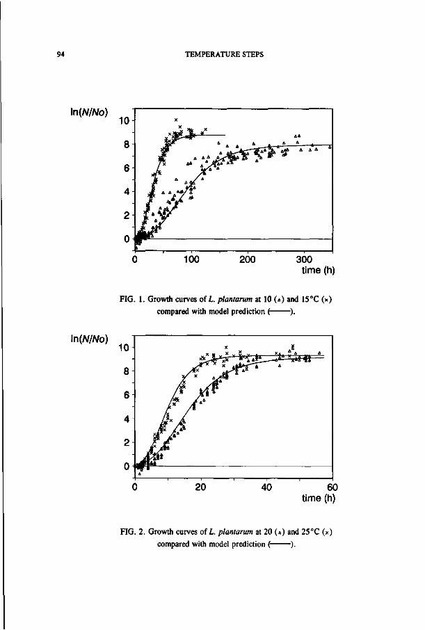
94 TEMPERATURE STEPS
\n(N/No) 10-
8
6
4
2
0
X
ÎSr 4 « , A « . 4 A A
/ X 44 4A J Ç 4 4 4 Ï^
/ 4V^ 4
i A **̂ S f , 4 Jf 4 4 4 ^ 4
je *j|»t
100 200 300 time (h)
FIG. 1. Growth curves of L. plantarum at 10 (4) and 15°C (x)
compared with model prediction ( ).
HNINo) 10
8
6
4
2
0 .
yfix
Jx jfc
rfî*É
4
/ x
x A
A*
X
^<r*J1
x)rx *-\Aï__
/*X »4-^S *
X ./IT
x*4 i A . *« * —-** X*4 TÎ4
4
20 40 60 time (h)
FIG. 2. Growth curves of L. plantarum at 20 (4) and 25°C (x)
compared with model prediction ( ).

CHAPTER 6 95
Temperature shift experiments. From the growth curves after the temperature shift
(r-f,), the lag time (A.5W/I) was estimated. This A.sW/, value was divided by the lag time
normally found at T2 to get the relative lag time ( \ * ). The three hypotheses can be tested by
plotting this relative lag time (X.*) versus r,* (Fig. 3, Table 2). Fig. 3 shows that the relative
lag time decreases if tt' goes from zero to one, and remains constant at higher t,' values.
Hypothesis 1 assumes that the relative lag time is equal to one in all cases. Fig. 3 shows that
the data do not support this assumption. Therefore, hypothesis 1 can be rejected.
Furthermore, it can be seen that most of the data are above the line predicted by hypothesis
2 ( a = 0) . This indicates that a temperature shift results in an additional lag phase. It was
already mentioned that this could be expected, since the cells will be stressed by the
temperature shift.
The a value was estimated by optimising the statistical acceptance of hypothesis 3 and
was found to be 0.2S, indicating that a temperature shift results in a new extra lag time ( \ x )
equal to one-fourth of the lag time normally found at the temperature after the shift (7"2).
\ 2.b
2
1.5
1
0.5-
0
0.5
0
o
0
V 1 A
v ! • • ° "o 1"'"* * Î
0
0
0 0 v
0
0
10
FIG. 3. Relative lag time (o ) plotted versus the relative time of shift, compared with model predictions. ( = hypothesis 1; = hypothesis 2; = hypothesis 3 with a =0.25).

96 TEMPERATURE STEPS
The three hypotheses were tested with the t test by calculating the confidence interval
of the estimated lag time of the growth data after the shift. For the various model predictions
it was tested whether the predictions are within this confidence interval. The experiments with
steps within the lag phase are given in Table 4 and the experiments with steps within the
exponential phase are given in Table 5.
TABLE 4. Results of temperature shifts within the lag phase
no"
LI L2 L3 14 L5 L6 L7 L8 L9
L10 L l l L12 L13 L14 L15 L16 L17 L18 L19 L20 L21 L22 L23 L24 L25 L26 L27 L28 L29 L30 L31 L32 L33 L34 L35 L36 L37 L38 L39 L40 L41 L42 L43 L44 L45 L46 L47 L48 L49 L50
r. 14.9 25.1 24.8 25.0 24.8 14.9 25.1 24.8 25.0 24.8 10.5 9.9 9.9 9.9 9.6
25.1 24.8 25.0 24.8 10.5 9.9 9.9 9.6 9.6
25.1 24.8 25.0 24.8 10.5 9.9 9.9 9.6 9.6
14.9 25.1 24.8 25.0 24.8 10.5 9.9 9.9 9.6 9.6 14.9 25.1 24.8 25.0 24.8 10.5 9.9
h 10.1 10.1 10.0 9.9 9.7 10.1 10.1 10.0 9.9 9.7
15.3 15.1 15.1 15.0 14.9 15.2 15.1 15.0 15.0 15.3 15.1 15.1 15.0 14.9 15.2 15.1 15.0 15.0 20.2 19.9 19.9 20.0 19.6 20.3 20.3 19.8 19.8 19.9 20.2 19.9 19.9 20.0 19.6 20.3 20.3 19.8 19.8 19.9 25.0 24.9
<s" 2.50 1.25 1.25 1.25 1.25 5.00 2.50 2.50 2.50 2.50 10.0 6.00 6.00 6.00 6.00 1.25 1.25 1.25 1.25 15.0 12.0 12.0 12.0 12.0 2.50 2.50 2.50 2.50 10.0 6.00 6.00 6.00 6.00 2.50 1.25 1.25 1.25 1.25 15.0 12.0 12.0 12.0 12.0 5.00 2.50 2.50 2.50 2.50 10.0 6.00
nc
17 15 18 18 21 17 15 18 18 21 13 12 14 16 17 12 14 17 18 12 11 14 15 16 12 12 16 17 15 14 14 16 16 13 14 14 13 14 12 12 11 13 13 13 13 13 13 15 13 11
\ ,
9.76 2.81 2.88 2.83 2.88 9.76 2.81 2.88 2.83 2.88
25.30 30.10 30.10 30.10 33.03 2.81 2.88 2.83 2.88
25.30 30.10 30.10 33.03 33.03 2.81 2.88 2.83 2.88
25.30 30.10 30.10 33.03 33.03 9.76 2.81 2.88 2.83 2.88
25.30 30.10 30.10 33.03 33.03 9.76 2.81 2.88 2.83 2.88
25.30 30.10
^
28.36 28.36 29.21 30.10 32.01 28.36 28.36 29.21 30.10 32.01 9.13 9.44 9.44 9.60 9.76 9.28 9.44 9.60 9.60 9.13 9.44 9.44 9.60 9.76 9.28 9.44 9.60 9.60 4.62 4.78 4.78 4.73 4.96 4.56 4.56 4.84 4.84 4.78 4.62 4.78 4.78 4.73 4.96 4.56 4.56 4.84 4.84 4.78 2.83 2.86
cf
0.256 0.445 0.434 0.442 0.434 0.512 0.891 0.868 0.883 0.868 0.395 0.199 0.199 0.199 0.182 0.445 0.434 0.442 0.434 0.593 0.399 0.399 0.363 0.363 0.891 0.868 0.883 0.868 0.395 0.199 0.199 0.182 0.182 0.256 0.445 0.434 0.442 0.434 0.593 0.399 0.399 0.363 0.363 0.512 0.891 0.868 0.883 0.868 0.395 0.199
X.S
15.11 11.43 6.90
11.09 16.77 21.52 6.95 5.28 7.79
12.83 8.92
10.80 11.23 11.43 8.45 8.11 8.01 8.22 6.30 9.22 7.43 9.45 6.39 5.50 4.47 4.08 4.47 3.55 3.91 5.06 6.56 6.58 4.28 4.64 3.87 4.23 4.96 4.23 4.64 2.12 5.47 4.63 3.87 4.77 2.54 1.59 2.56 2.11 3.19 3.54
minh
4.31 -0.60 -4.57 -0.24 6.85 9.88 -2.99 -5.32 -2.52 3.94 5.00 6.46 7.39 7.65 4.57 4.26 4.23 4.51 2.62 5.18 3.01 5.80 2.55 1.70 0.69 0.50 0.90 -0.25 2.32 3.25 4.49 4.57 2.46 2.33 1.96 2.33 2.94 2.35 2.57
-0.28 2.52 1.86 1.21 2.08 0.54
-0.24 0.71 0.39 1.96 2.17
raaxh
25.91 23.45 18.37 22.43 26.69 33.15 16.89 15.88 18.11 21.71 12.85 15.15 15.06 15.20 12.34 11.97 11.79 11.93 9.98
13.25 11.85 13.09 10.24 9.30 8.24 7.66 8.04 7.34 5.51 6.86 8.63 8.58 6.09 6.96 5.77 6.14 6.97 6.11 6.72 4.52 8.42 7.41 6.53 7.46 4.54 3.41 4.41 3.84 4.42 4.91
a = 0 j
21.10 15.73 16.54 16.81 18.12 13.84 3.09 3.87 3.52 4.24 5.52 7.56 7.56 7.69 7.99 5.15 5.34 5.36 5.43 3.72 5.68 5.68 6.11 6.22 1.01 1.25 1.12 1.27 2.79 3.83 3.83 3.87 4.06 3.40 2.53 2.74 2.70 2.71 1.88 2.88 2.88 3.01 3.16 2.23 0.50 0.64 0.57 0.63 1.71 2.29
I k
28.19 22.82 23.84 24.34 26.13 20.93 10.18 11.17 11.04 12.24 7.80 9.92 9.92
10.09 10.43 7.47 7.70 7.76 7.83 6.00 8.03 8.03 8.51 8.66 3.33 3.61 3.52 3.67 3.95 5.03 5.03 5.05 5.30 4.54 3.67 3.95 3.91 3.91 3.03 4.07 4.07 4.19 4.40 3.37 1.64 1.85 1.78 1.83 2.42 3.00

CHAPTER 6 97
TABLE 4 continued.
no"
L51 L52 L53 L54 L55 L56 L57 L58 L59 L60 L61 L62 L63 L64 L65 L66 L67 L68 L69 L70 L71
Ti
9.9 9.6 9.6
14.9 20.2 10.5 9.9 9.9 9.6 9.6 14.9 20.2 10.2 10.2 4.0 4.0 14.0 14.0 14.7 14.7 20.0
Tl
24.9 25.0 24.7 25.1 25.1 25.0 24.9 24.9 25.0 24.7 25.1 25.1 30.7 30.7 20.0 35.0 24.0 24.0 20.0 20.0 30.0
's" 6.00 6.00 6.00 2.50 1.33 15.0 12.0 12.0 12.0 12.0 5.00 2.67 19.5 24.0 1873 1873 5.25 2.25 5.00 2.50 2.50
rf
14 12 15 12 15 13 10 11 12 12 10 13 11 10 22 18 16 17 16 16 8
*•!
30.10 33.03 33.03 9.76 4.62
25.30 30.10 30.10 33.03 33.03 9.76 4.62
27.55 27.55 2616 2616 11.47 11.47 10.11 10.11 4.73
\2*
2.86 2.83 2.91 2.81 2.81 2.83 2.86 2.86 2.83 2.91 2.81 2.81 1.86 1.86 4.73 1.57 3.10 3.10 4.73 4.73 1.94
'." 0.199 0.182 0.182 0.256 0.288 0.593 0.399 0.399 0.363 0.363 0.512 0.578 0.708 0.871 0.716 0.716 0.458 0.196 0.495 0.247 0.529
\ s
3.94 3.98 3.05 3.68 1.95 1.79 3.94 4.34 6.11 2.86 2.18 2.80 1.57 1.13
22.56 15.14 3.64 5.58 4.48 4.95 1.50
minh
2.69 2.66 1.84 2.46 1.01 0.43 1.48 1.49 2.14 0.95 0.63 1.65 0.82 0.27
19.83 14.11 1.43 3.55 2.57 2.94 0.29
maxh
5.18 5.29 4.27 4.89 2.88 3.14 6.40 7.18 10.09 4.77 3.73 3.95 2.33 1.99
25.30 16.16 5.85 7.62 6.39 6.95 2.71
a = 0 j
2.29 2.32 2.38 2.09 2.00 1.15 1.72 1.72 1.80 1.85 1.37 1.18 0.54 0.24 1.34 0.45 1.68 2.49 2.39 3.56 0.91
l k
3.00 3.02 3.11 2.79 2.70 1.86 2.43 2.43 2.51 2.58 2.07 1.89 1.01 0.70 2.52 0.84 2.46 3.27 3.57 4.74 1.40
"Experimental number, bold code = curve plotted in graph (Fig. 4 to 13);bfs= time of shift (h); °n= number of datum points in growth curve; d bold value indicates that hypothesis 1 is accepted by t test; ffs*=?s/\,; t\= estimated lag time from growth data; hmin, max = minimum and maximum 95% confidence limit of lag time, 95% confidence intervals are calculated with f =1.96 (at infinite degrees of freedom, the variance of the measuring error was calculated with 646 datum points); ' bold value indicates that hypothesis 2 is accepted by t test; k bold value indicates that hypothesis 3 is accepted by t test.
Table 4 shows that hypothesis 1 and hypothesis 2 are accepted for most of the
experiments and hypothesis 3 is accepted for almost all experiments.
In two cases (curves L65 and L66) there were very large deviations between the
confidence interval of the measured lag phase duration and the model predictions. In Fig. 4
the data for these temperature shift experiments are plotted. The kinetic behaviour appears to
be reasonably well predicted, except for the dying during incubation at 4°C. However, if the
time axis of the part of the curve after the temperature shift is extended (Fig. 5), it can be
seen that the predicted lag time is much smaller than the actual lag time. In these experiments
the first incubation is around the minimal temperature of growth [Tmia value is 3.29°C (Table
1)]. Incubation at very low temperatures (around or below 7"min) may be damaging to the cells,
resulting in (slow) dying, and increased lag times, when transferred to higher temperatures.
More work is needed to quantify these effects. These two experiments will not be taken into
account for the following. For no other cases a significant effect could be found resulting from
the time of the shift, the first or second incubation temperature, or the size of the step.

98 TEMPERATURE STEPS
ln(/V/Ato) 10
8
1500 2000 time (h)
FIG. 4. Growth curve with a shift from 4°C to 20 (L65) and 35°C (L66) at 1873 h compared with model prediction (• , = 20°C; + , = 35°C).
\n(N/No) 1 0
1900 1950 2000 time (h)
FIG. 5. Growth curve after a shift from 4°C to 20 (L65) and 35°C (L66) at 1873 h compared with
model prediction (• , = 20°C; • , = 35°C).
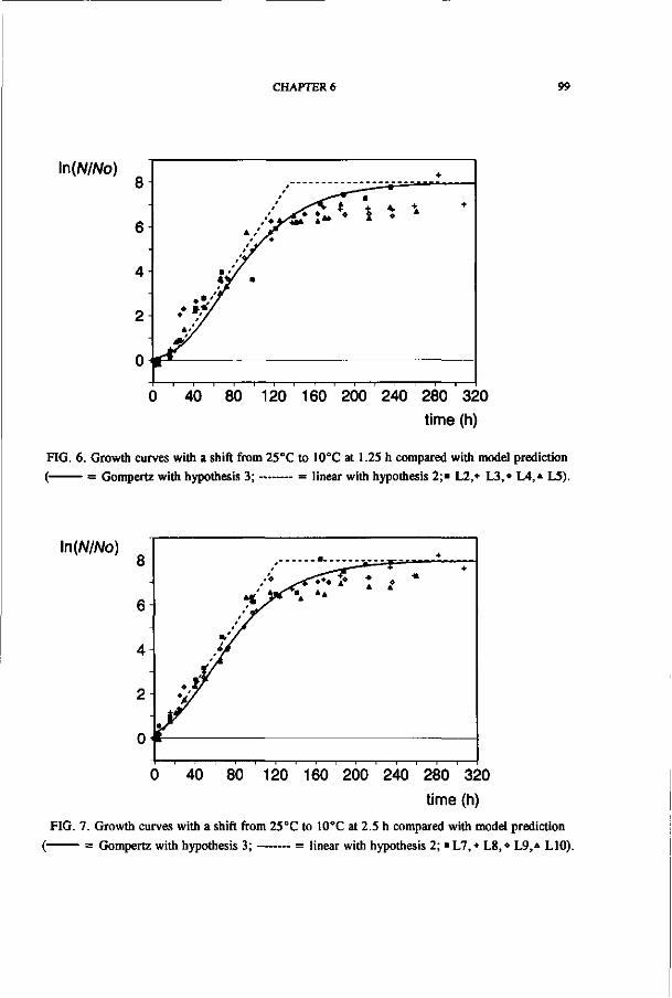
CHAPTER 6 99
ln(A//Afo)
-I 1 1 r-0 40 80 120 160 200 240 280 320
time (h)
FIG. 6. Growth curves with a shift from 25CC to 10°C at 1.25 h compared with model prediction ( = Gompertz with hypothesis 3; = linear with hypothesis 2;» L2,+ L3,» L4,* L5).
\n(N/No)
0 40 80 120 160 200 240 280 320
time (h)
FIG. 7. Growth curves with a shift from 25°C to 10°C at 2.5 h compared with model prediction
( = Gompertz with hypothesis 3; = linear with hypothesis 2; "L7,+ L8, • L9,* L10).

100 TEMPERATURE STEPS
TABLE 5. Results of temperature shifts within the exponential phase
no"
El E2 E3 E4 E5 E6 E7 E8 E9
E10 E l l E12 E13 E14 E15 E16 E17 E18 E19 E20 E21 E22 E23 E24 E25 E26 E27 E28 E29 E30 E31 E32 E33 E34 E35 E36 E37 E38 E39 E40 E41 E42 E43 E44 E45 E46 E47 E48 E49 E50 E51 E52 E53
Tl
8.9 8.9 8.9 8.9
14.0 14.0 14.0 14.0 14.0 14.0 14.7 14.7 14.7 14.7 14.7 14.7 16.7 16.7 16.7 16.7 18.0 18.0 18.0 18.0 40.8 40.8 9.0 8.0
11.7 14.2 14.2 14.5 14.5 14.5 15.3 15.0 16.6 16.8 20.2 25.0 25.0 25.0 25.0 25.0 26.0 30.7 30.6 35.0 35.0 35.0 35.0 35.0 35.0
Ti
14.2 16.5 17.8 20.1 24.0 24.0 24.0 24.0 24.0 24.0 20.0 20.0 20.0 20.0 20.0 20.0 10.4 12.5 14.6 18.8 13.9 22.1 13.9 22.1 25.0 25.0 14.0 20.7 16.6 17.3 20.5 24.8 30.3 34.8 30.5 25.0 11.7 8.0 8.0
14.2 17.3 18.9 9.0
11.0 36.8 10.1 10.5 20.0 20.0 25.0 25.0 30.0 30.0
',b
119 119 119 119
72.5 70.0 43.0 25.0 20.0 17.5 64.5 43.0 24.0 19.0 16.0 13.5 26.5 26.5 26.5 26.5 20.0 20.0 32.0 32.0 18.0 3.50 50.5 70.0 22.5 18.5 18.5 20.0 20.0 20.0 19.0 22.0 22.5 20.0 20.0 4.50 4.50 4.50 6.50 6.50 3.00 2.00 3.00 2.00 6.00 2.50 6.00 2.00 6.00
nc
21 17 17 17 15 17 6 11 12 14 15 14 14 16 16 17 16 16 15 15 21 17 16 12 10 13 15 8
14 11 12 12 11 10 5 9 17 15 15 10 10 10 28 26 9 9 8 9 6 10 6 11 6
X,
41.79 41.79 41.79 41.79 11.47 11.47 11.47 11.47 11.47 11.47 10.11 10.11 10.11 10.11 10.11 10.11 7.32 7.32 7.32 7.32 6.09 6.09 6.09 6.09 2.35 2.35
40.34 59.29 18.60 11.06 11.06 10.47 10.47 10.47 9.13 9.60 7.43 7.22 4.62 2.83 2.83 2.83 2.83 2.83 2.60 1.86 1.87 1.57 1.57 1.57 1.57 1.57 1.57
^ d
11.06 7.55 6.26 4.67 3.10 3.10 3.10 3.10 3.10 3.10 4.73 4.73 4.73 4.73 4.73 4.73
26.02 15.51 10.29 5.48 11.69 3.74
11.69 3.74 2.83 2.83 11.47 4.36 7.43 6.71 4.46 2.88 1.91 1.58 1.88 2.83 18.60 59.29 59.29 11.06 6.71 5.41
40.34 22.13 1.57
28.36 25.30 4.73 4.73 2.83 2.83 1.94 1.94
cf
2.848 2.848 2.848 2.848 6.320 6.102 3.748 2.179 1.743 1.525 6.380 4.254 2.374 1.879 1.583 1.335 3.618 3.618 3.618 3.618 3.284 3.284 5.254 5.254 7.653 1.488 1.252 1.181 1.210 1.673 1.673 1.910 1.910 1.910 2.082 2.292 3.027 2.772 4.331 1.590 1.590 1.590 2.296 2.296 1.155 1.075 1.603 1.272 3.817 1.590 3.817 1.272 3.817
As
4.51 4.82 3.00 2.70 -0.22 0.56 0.49 0.92 0.67 0.35 1.04 1.09 1.77 1.19 1.17 1.27 7.75 4.93 5.29 3.07 7.99 1.71 2.36 1.70 0.47 2.27 6.69 4.04 4.44 2.52 1.75
-0.01 -0.13 0.17 0.24 0.67 0.15 14.22 1.69 4.15 1.16 1.22
24.71 0.06 0.31 10.35 5.47 -0.71 -0.04 0.24 0.04 -0.11 -0.13
minh
1.39 2.33 0.94 1.10
-1.77 -0.92 -1.27 -0.26 -0.53 -0.93 -1.10 -0.85 -0.25 -0.31 -0.28 -0.23 -0.86 -0.85 0.82 0.28 4.34 0.14
-3.17 -1.09 -1.68 0.74 -0.07 1.78 0.07 1.13 0.39 -1.25 -1.02 -0.58 -1.48 -0.47 -9.97 -9.36
-34.30 -0.73 -2.11 -1.28 8.05
-7.48 -0.36 1.04
-5.36 -2.21 -1.68 -0.90 -1.06 -0.74 -1.12
max'
7.63 7.31 5.06 4.30 1.33 2.04 2.25 2.10 1.88 1.62 3.18 3.04 3.80 2.69 2.62 2.78
16.36 10.71 9.76 5.85 11.64 3.27 7.89 4.50 2.63 3.80
13.46 6.30 8.80 3.91 3.11 1.23 0.76 0.92 1.97 1.81
10.26 37.79 37.68 9.02 4.43 3.72
41.37 7.61 0.98 19.65 16.30 0.79 1.60 1.38 1.13 0.52 0.87
Ik
2.76 1.89 1.56 1.17 0.78 0.78 0.78 0.78 0.78 0.78 1.18 1.18 1.18 1.18 1.18 1.18 6.50 3.88 2.57 1.37 2.92 0.94 2.92 0.94 0.71 0.71 2.87 1.09 1.86 1.68 1.11 0.72 0.48 0.39 0.47 0.71 4.65
14.82 14.82 2.76 1.68 1.35
10.08 5.53 0.39 7.09 6.33 1.18 1.18 0.71 0.71 0.49 0.49
"Experimental number, bold code = curve plotted in graph (Fig. 10 to 13); bfs= time of shift (h); cn= number of datum points in growth curve; d bold value indicates that hypothesis 1 is accepted by t test; ftt'=tJ\, ; 6 X- = estimated lag time from growth data; hmin= minimum 95% confidence limit of lag time, bold value indicates that a = 0 is within the confidence interval (hypothesis 2); 'max = maximum 95% confidence limit of lag time, 95% confidence intervals are calculated with f =1.96 (at infinite degrees of freedom, the variance of the measuring error was calculated with 646 datum points); k bold value indicates that hypothesis 3 is accepted by t test.

CHAPTER 6 101
Table 5 shows that hypothesis 1 is accepted for only a few experiments. Hypothesis 2
is accepted for most of the experiments and hypothesis 3 is accepted for almost all
experiments.
In Table 6 the total number of accepted cases of each hypothesis is given for all curves
(except for the curves L65 and L66). Table 6 shows that hypothesis 1 is accepted only in 47%
of the cases and does not appear to be appropriate (see also Fig. 3). Hypothesis 2 is accepted
in most of the cases (73%) and hypothesis 3 is accepted in almost all cases (93%). Therefore,
hypothesis 3 appears to be the most appropriate.
TABLE 6. Acceptance rates of the three hypotheses (% between brackets)
Hypothesis Lag phase Exp. phase Total
1
2
3
49 (71)
51 (74)
65 (94)
8(15)
38 (72)
48 (91)
57 (47)
89 (73)
113(93)
Total 69 53 122
Predictions compared with experiments. Now the measured data can be compared to
the model predictions. For several temperature shift experiments growth data and model
predictions (following hypothesis 3 with a = 0 .25) are compared. For shifts within the lag
phase examples are given in Fig. 6 to 9. The model predictions have been calculated using
equations 12 and 13 (see Appendix). Curves L3 and L4 are examples for which hypothesis 3
was rejected.
In Fig. 10 to 13 results of temperature changes at different times are given. For shifts
within the exponential phase the model predictions have been calculated with equations 14 and
15 (see Appendix). It can be seen that the predictions agree very well with the measured data.
It should be noted that the predictions arise from models based on earlier growth data (6) at
constant temperature, so no fitting occurred.
Hypothesis 2 was accepted in many cases (73%) and for simulation purposes this
assumption is more convenient, especially if there are many temperature changes during the
shelf life of a product or during dynamically changing temperatures. In Fig. 8 and 9 the
predictions using this assumption ( a = 0) are also given. It can be seen that this model also
describes the kinetic behaviour of the data well enough for a number of practical applications.
Curves L51, L52, and L59 are examples for which hypothesis 2 was rejected, for temperature
shifts within the lag phase.
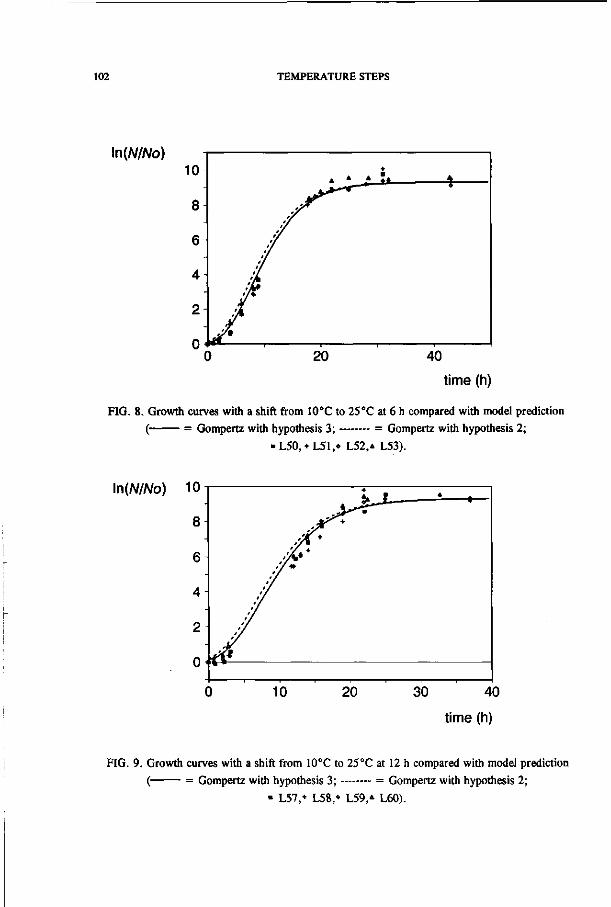
102 TEMPERATURE STEPS
\r\(N/No)
time (h)
FIG. 8. Growth curves with a shift from 10°C to 25°C at 6 h compared with model prediction
( = Gompertz with hypothesis 3; = Gompertz with hypothesis 2;
• L50. + L51,» L52,* L53).
ln(A//A/o) 10
10 20
V +
4 ,</
2 //
0 ^ -
30 40
time (h)
FIG. 9. Growth curves with a shift from 10°C to 25°C at 12 h compared with model prediction
( = Gompertz with hypothesis 3; = Gompertz with hypothesis 2;
• L57,+ L58,» L59 / L60).

CHAPTER 6 103
HN/No) 1 4 I I -
12
10
8
6
4
2
0^
(
1
t 1 A
1 /
»IK
IL If
j/A k
j^3r • / •
^<"E
' / if
if if
m i y1^ t f , - - ^ - - - - * - - - - -
f £>"^~~ 3 •'M''
J' / •
• ^
) 20 40 60 80 100 120 time (h)
FIG. 10. Growth curves with shifts from 14°C to 24°C compared with model prediction
( = Gompertz with hypothesis 3; = linear with hypothesis 2;
-E5.+ E7,» E9,»L67).
In(WAfo) I H -
12
10
8
6
4
2
0^
*s*w^
' & ' / J ' ¥ ' / ' / 'd 7 'A
if if if i L J if
'L i f
»7 / i if l a
f WEM
* * • " • * f a .1 . 'Y*/ ^-*~~~—
T ^ S ^ * ^ rmS^
'X a
/m
•
20 40 60 80 100 120 140
time (h)
FIG. 11. Growth curves with shifts from 14°C to 24°C compared with model prediction
( = Gompertz with hypothesis 3; = linear with hypothesis 2;
•E6,*E8,« E10,* L68).

104 TEMPERATURE STEPS
ln(A//A/o) 14
12
10
fi
6 -
4 "
2
n U
L / A /
/ 1*1 / r *&
J Mar
Jf
//Y* / /+ / V+ y
/ / B
/ ^ # / •
/ •
ySW
#
1-• . •
'*' 20 40 60 80 100 120
time (h)
FIG. 12. Growth curves with shifts from 15°C to 20°C compared with model prediction
( = Gompertz with hypothesis 3; • El 1, + E13, »E15, * L69).
\r\(N/No)
100 120 time (h)
FIG. 13. Growth curves with shifts from 15°C to 20°C compared with model prediction
( = Gompertz with hypothesis 3; • E12, • E14, « E16, *L70).

CHAPTER 6 105
By using both hypotheses 2, and the linear growth model (equation 1) instead of the
modified Gompertz model, the calculations become easier. The predictions of the linear
model (with the use of hypothesis 2) are compared with the modified Gompertz model (with
hypothesis 3), in Fig. 6, 7, 10 and 11. Curve L68 is an example for which hypothesis 3 was
rejected. The linear model gives comparable results to the modified Gompertz model, only
where the growth curve bends off towards the asymptote, the linear model fails to describe
the data. The asymptotic level [ln(JV/A/„)]is dependent strongly on the inoculum level,
and shows often large experimental error (6, 8). Moreover, the asymptotic level is often of
no real practical importance, since food products are generally spoiled, before the asymptotic
level is reached. For a number of applications the global kinetic behaviour will be sufficient
and the linear model could be chosen, since this model has the advantage of simplicity.
CONCLUSIONS
It can be assumed that temperature shifts within the lag phase can be handled by adding
relative parts of the lag time still to be completed and that temperature shifts within the
exponential phase result in no additional lag. These two assumptions were accepted
statistically in more than 70% of the experiments. The kinetic behaviour was well predicted
using these assumptions. The hypothesis that a temperature shift results in an additional lag
phase of one-fourth of the lag time normally found at the second temperature is accepted in
more than 90% of the experiments. This observation shows that the bacteria are exposed to
stress by a shift in temperature in the lag phase as well as in the exponential phase.
With this knowledge growth curves can be predicted with the modified Gompertz
equation. For a number of practical applications the procedure can be simplified by neglecting
the additional lag time. Also the linear growth equation predicts data within a certain range
and therefore can be preferred when simplicity of the function is preferred.
Shifts of temperature around the minimum temperature of growth showed firstly dying
of the cells and secondly very large deviations compared to the model prediction. This
observation indicates the need for more experimental work around the minimum temperature
of growth.
ACKNOWLEDGMENTS
This work was partly funded by Unilever research lab Vlaardingen. The authors wish to thank P.M. Klapwijk, J.P.P.M. Smelt, and P.F. ter Steeg for valuable discussions. The authors wish to thank L.A. Ledelay, B.A. Campfens, and E.W. Oosterom for carrying out most of the experiments.

106 TEMPERATURE STEPS
REFERENCES
1. Fu, B., P.S. Taoukis, and T.P. Labuza. 1991. Predictive microbiology for monitoring
spoilage of dairy products with time-temperature integrators. J. Food Sei. 56:1209-1215.
2. Langeveld, L.P.M., and F. Cuperus. 1980. The relation between temperature and growth rate
in pasteurized milk of different types of bacteria which are important to the deterioration of that
milk. Neth. Milk Dairy J. 34:106-125.
3. Ng, H., J.L. Ingraham, and A.G. Marr. 1962. Damage and derepression in Escherichia coli
resulting from growth at low temperatures. J. Bacteriol. 84:331-339.
4. Shaw, M.K. 1967. Effect of abrupt temperature shift on the growth of mesophilic and
psychrophilic yeasts. J. Bacteriol. 93:1332-1336.
5. Simpson R., K.Y. Li, and J.A. Torres. 1989. A management tool to improve the microbial
quality of refrigerated foods, p. 155-168. In Proceedings of an international conference on
technical innovations in freezing and refrigeration of fruits and vegetables, University of
California, Davis USA Publ. International Institute of Refrigeration.
6. Zwietering, M.H., H.G.A.M. Cuppers, J.C. de Wit, and K. van 't Riet. 1993. Evaluation
of data transformations and validation of models for the effect of temperature on bacterial
growth. Chapter 5 of this thesis.
7. Zwietering, M.H., I. Jongenburger, F.M. Rombouts, and K. van 't Riet. 1990. Modeling
of the bacterial growth curve. Appl. Environ. Microb. 56:1875-1881. Chapter 2 of this thesis.
8. Zwietering, M.H., J.T. de Koos, B.E. Hasenack, J.C. de Wit, K. van 't Riet. 1991.
Modeling of the bacterial growth as function of the temperature. Appl. Environ. Microb.
57:1094-1101. Chapl T 4 of this thesis.
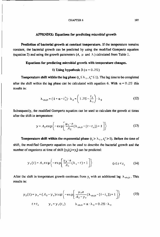
CHAPTER 6 107
APPENDIX: Equations for predicting microbial growth
Prediction of bacterial growth at constant temperature. If the temperature remains
constant, the bacterial growth can be predicted by using the modified Gompertz equation
(equation 2) and using the growth parameters (A, [i and A.) calculated from Table 1.
Equations for predicting microbial growth with temperature changes.
1) Using hypothesis 3 ( a = 0 .25)
Temperature shift within the lag phase (rs < A t , fs* S 1). The lag time to be completed
after the shift within the lag phase can be calculated with equation 6. With a = 0 .25 this
results in:
^ w / ( = ( l + a - U ' ^ 2 = 1-25-\ ,
(12)
Subsequently, the modified Gompertz equation can be used to calculate the growth at times
after the shift in temperature:
y = /42exp< - e xp H2 '
e
A, ( ^ s / , 1 / ( - [ f - ' s ] ) + l (13)
Temperature shift within the exponential phase (fs> X ! , tt' > 1). Before the time of
shift, the modified Gompertz equation can be used to describe the bacterial growth and the
number of organisms at time of shift ty,(0 =yj can be predicted:
yl(t) = Alexp{ - e xp M - x - e
( \ , - 0 + l 0 < t < ( , (14)
After the shift in temperature growth continues from ys with an additional lag X shift. This
results in:
y 2 ( 0 = y s + ( / 4 2 - y s ) exp - e xp
^ e • ( k , W / , - [ t - U ) + i
A2-ys
t>ts y s = y i ( ' s ) \sllifl = a-\2 = 0.25-\2
(15)

108 TEMPERATURE STEPS
2) Using hypothesis 2 (a = 0)
Temperature shift within the lag phase (t, < X,, t,' < 1). The lag time to be completed
after a shift within the lag phase can be calculated by assuming a = 0 in equation 6:
^ s M f t - ^ + oi-ts)-X2-^\-—j-X2 (16)
Subsequently, the modified Gompertz equation (equation 13) can be used to calculate the
growth at times after the shift in temperature.
Temperature shift within the exponential phase (ts> Ky , ?s*> 1). The number of
organisms before the time of shift can be predicted by equation 14. The number of organisms
after the time of shift can be predicted by:
y 2 ( 0 = y , + M 2 - y s ) e x p \ - e x p i i 2 e
( - [ t - t . ] ) - l (17) A2-y
t>t, y , = y i ( U
3) Using linear growth
It will be even more convenient to use linear growth and hypothesis 2 ( a = 0) .
Temperature shift within the lag phase (rs < K,, t,' < 1). The lag time to be completed
after a shift within the lag phase can be calculated by equation 16. After the lag time is
completed exponential growth will occur until the asymptote is reached:
y = o t-ts<\shift
y = H 2 - ( ' - t s - k s h i / i ) Xstull<t-ts<A2/Vi2 + KshLn (18)
y = ^ 2 t-ts>A2/\i2 + \s>l,f,

CHAPTER 6 109
Temperature shift within the exponential phase (ta> K-i, f„*>l). The number of
organisms before the time of shift can be predicted by:
(19)
(20)
y = 0 t<\t
y - u , - ( t - \ , ) \x<t<t,
and the growth after the time of shift (ta) results in:
y - m - C t . - k ^ + u ^ C t - t . ) ts<t<Az l i l ' i t s Kl) + ts
t A2-Vi- ( t s - ^ i ) t y = A2 t> + ts 1*2
This equation can be expanded very easily to more temperature shifts.
Various temperature shifts. If many temperature shifts occur or during dynamically
changing temperature conditions it will be better and easier to use hypothesis 2 ( a = 0) and
linear growth. The modified Gompertz equation is far to complex to be used with many shifts.
Temperature shift within the lag phase. The lag time to be completed after many
shifts within the lag phase can be calculated by assuming a = 0 in equation 6 and adding all
relative parts of the lag time that are completed until one is reached:
4> = ) —- until * = 1 (21)
or for dynamically changing temperatures:
4>= f ^ until *= 1 (22) J A.

110 TEMPERATURE STEPS
Temperature shift within the exponential phase. As soon as * = 1 the exponential
phase sets in. The time at which <i> = 1 is defined as £+.
y = M-iC«s i - f • ) + M ' s z ~ t s l ) + \i3(t-1s2)
, , , A-V-i(tsl-tt)-[i2(ts2-tsl) t*2
(23) y = 0 t<tt
y - u , - ( t - t # ) «*<«<«,/
and the growth after the first time of shift (f9l) in the exponential phase results in:
y = Vi(ts]-t*) + ii2(t-ts]) tsl<t<tsZ (24)
and the growth after the second time of shift (fs2) in the exponential phase results in:
(25)
until the asymptote is reached:
y = A t> + ts2 (26) M-3

CHAPTER 7
A DECISION SUPPORT SYSTEM FOR PREDICTION OF THE MICROBIAL SPOILAGE IN FOODS
ABSTRACT
A method was developed to combine qualitative and quantitative information to predict
possible growth of microorganisms in foods. The pH, water activity, temperature, and
oxygen availability of foods are coupled to the growth characteristics of microorganisms.
Therefore, a database with characteristics of foods and a database of kinetic parameters of
microorganisms were built. In the first database, a tree structure based on physical similarity
was built, for the case that information about the characteristics of a particular food is
unknown. The product information can be estimated by comparing with similar products at
the same level of the tree or the level above. A method is developed to make an estimation of
the microbial growth kinetics on the basis of models. This is done by introducing a growth
factor, which can be calculated on the basis of readily available data from literature. Since all
the information can be altered, the system can give better predictions when more and more
accurate information is added.
INTRODUCTION
Food Quality. Food quality can be defined as the sum of the characteristics of a food
that determines the satisfaction of the consumer and compliance to legal standards. Thus,
food quality is a combination of numerous factors, such as organoleptic properties (e.g.,
texture, flavor, color), nutritional value (e.g., caloric content, fatty acid composition), and
safety conditions (e.g., microbial number, toxins, hormones). Some of these factors (e.g.,
microbial numbers) can be quantified relatively easily, others (e.g., flavor) are very difficult
to assess quantitatively. Food quality thus cannot be quantified in every detail, and overall
This chapter has been published as:
A Decision Support System for Prediction of the Microbial Spoilage in Foods
M.H. Zwietering, T. Wijtzes, J.C. de Wit, and K. van 't Riet (1992)
J. Food Prot. 55:973-979

112 MICROBIAL SPOILAGE PREDICTION
quantification depends strongly on the priority of the different aspects determining the quality.
To determine the total food quality, quality indicators are needed and must be weighted,
depending on the product, trends, producer, and market.
Food quality is gaining more and more interest for a number of reasons. The food
market deals in most cases with satiation; therefore, quality becomes more important than
quantity. There are new quality attributes which are highly appreciated by the modern
consumer (in contrast to traditional quality demands). Consumers show an increasing interest
in convenience foods with the appearance and taste of fresh products and food quality aspects
such as flavor and (assumed) health aspects (e.g., nutrition, fatty acid quantity and
composition, energy content, salt concentration, additives, such as preservatives).
Prediction of the kinetics of possible quality loss is important for the following reasons.
Consumers are willing to pay a higher price for quality. The manufacturer wants to produce
constant quality products at the lowest costs. Many products have a limited shelf life.
Production and storage conditions affect quality very strongly; therefore, production and
distribution are often critical. From the past there are many dried, salted, frozen, and
sterilized products, while nowadays chilled and intermediate-moisture foods are becoming
more important. The shelf life of a product should match the distribution regime: daily
delivery for perishable products such as fresh milk, bread, fresh vegetables, and fresh meat,
or less frequently as for salads, margarine, etc. Distribution routes have become longer, and
therefore, there is a need for an increase in shelf life. In some areas there is a rather rapid
product development (changes in product formulation). Consequently, it will be very useful
to make an estimation of the shelf life during product development. Formulation of products
may be different in different countries or regions, because of legal requirements or regional
food preferences. Therefore, it would be useful to know the effects of different compositions
on the shelf life, so that each formulation does not require a laborious shelf-life test.
New techniques are being developed to meet these quality demands, such as new
technologies (e.g., microwave, ultrahigh temperature processes, modified atmosphere
packaging, irradiation), and new strategies (e.g., logistics, and modeling).
Quality loss. Quality loss can be a result of microbial, chemical, enzymatic, or physical
reactions. Different factors influence quality loss, such as the composition of the product, and
the processing and storage conditions. Deterioration reactions may occur when the physical
variables of the product are within the range of the specific reaction. For quantification of the
reaction rate, the kinetics of the reaction should be known. This can be done by models that
include the range in which spoilage can occur and the physical variables of the product. As

CHAPTER 7 113
soon as good models are available and values for the physical variables are estimated, the rate
of spoilage processes can be predicted. The resulting quantitative estimation can be compared
with quality parameters.
A considerable amount of research has been conducted on the deterioration of food
(e.g., 2, 10). This research yielded a large amount of quantitative data. Also, much qualitative
information is available. Yet, for a quantitative prediction of the quality of a given food
product, there are often not enough data, or the data show too large a measuring error to be
used. It is difficult to combine a broad range of information, from qualitative to quantitative.
However, it will be very useful to combine all this information in a structured manner, to
predict product quality in the best possible way.
The objective of this work is to develop a system in which quantitative data can be
combined in a structured manner with qualitative data, quantitative information, and models.
Such a system would be a useful tool in product development, predicting possible spoilage
and estimating the kinetics of possible deterioration. As soon as more data, knowledge, or
new models are gathered, this can be added, resulting in more valuable predictions.
SYSTEM STRUCTURE
The system. A system was developed that determines the possible growth of
microorganisms on a certain food product. Numerous factors can influence growth. From the
most important factors, pH, water activity (aw), temperature (7), and oxygen availability are
taken into account. These physical properties of the product are compared with the properties
of the microorganisms (Fig. 1). The physical variables of various foods are collected in a
database (database 1) as are the growth data of microbes (database 2). The data for each
microorganism are matched with the physical variables of the food product, by simply
determining if the physical variables of the product are within the growth limits of that
microorganism ("pattern matching"). For these organisms, an estimate of the growth rate is
calculated on the basis of the value of the physical variables. The estimation of growth is
carried out by using models that describe growth over the range of physical variables.
The list of organisms that may spoil the product is sorted by growth rate. This list can
be altered by applying rules to diminish the number of organisms in the list or to improve the
value of the predictions. Some of these rules are dependent on the product, some on the
properties of organisms, and some are of general application. In this way the final list of
organisms is obtained, which is now based on physical variables of the product, growth
parameters of microorganisms, models, and qualitative reasoning.

114 MICROBIAL SPOILAGE PREDICTION
database 1 database 2
physical parameters
Foods (components)
pH,aw , T, O,
kinetics: m.o.
"
matching — i ^ knowledge — * • estimate of growth rate
FIG. 1. Structure of the system.
TABLE 1. An example of the information stored in the product database
Name Identification code Temperature (7) PH
Oxygen availability
yogurt S.A.B.A.C 5 4.2 0.990 no oxygen
It should be noted that spoilage of a product will only occur if an organism is present
and able to grow in that product. Until now it is assumed that all organisms can be present
everywhere. This can result in predictions of growth of organisms that are unlikely to be
present in such a product. Therefore, knowledge of the presence of organisms on certain
products can be included in the information database. Another possibility is that the usual
microflora of products is included in the food database. However, organisms that up to now
have not caused problems in a product are often not known to be present in a product. If the
composition or processing of such a product is changed, these organisms may start to cause
problems. Therefore, it is assumed that all organisms can be present everywhere.

CHAPTER 7 115
Food database. Database 1 (Fig. 1) contains the physical variables of different foods,
as shown in Table 1. The physical variables are known only for a limited number of products.
The remainder contains name and identification code (I.D.). The I.D. of a product determines
the position of the product in the classification tree (Fig. 2). The first letter (S) stands for
food, addition of the second for the first subdivision of food [dairy (S.A), bakery (S.D),
vegetables (S.F), meat (S.H), etc.]. These groups of products are divided by addition of the
third letter of the I.D., etc.
fresh milk skim milk (S.A.A.A) (S.A.A.C)
cheese (S.A.B.C)
buttermilk (S.A.B.A.A) yoghurt (S.A.B.A.C)
FIG. 2. Structure of database 1, in which foods are sorted by their physical characteristics.
The number of food products is more or less infinite and, as may be expected, not all
the physical variables of all different foods are known. Therefore, the database is structured
in such a way that the products are sorted with respect to their physical properties so that foods
that are grouped together are closely related (Fig. 2). The classification system proposed by
Jowitt (4) based on the physical properties of foods is therefore used. In such a way, missing
information, even when a product is absent, can be substituted with knowledge from
comparable products.
Moreover, the physical variables can always be altered. If comparable products are not
found, estimated variables can be entered.

116 MICROBIAL SPOILAGE PREDICTION
Organism database. A database is built for microorganisms, to contain the information
as given in Table 2. The database contains the name of the organism and the growth ranges
of the physical variables: oxygen requirement, the minimum and maximum pH, aw, and
temperature. Additionally, the optimum growth rate and the optimum values of pH and
temperature are stored to be used in kinetic models. Furthermore, the Gram staining, type,
and spore-forming abilities are stored to be used for further selection procedures (qualitative
reasoning) or future use. The possibility exists to alter all information.
TABLE 2. An example of the information stored in the organism database
Genus Pseudomonas
Species putida
Oxygen necessity aerobic
Type (bacterium, yeast, mould) bacterium
Gram stain (only for bacteria) negative
Spore forming no
T: min max opt -8 43 30
pH: min max opt 4.7 8.5 7.8
aw: min max opt* max 0.96 1.000
optimum growth rate (jar1) 1
Selection of organisms that can grow on a particular product. As soon as the
physical variables of a product are known, a matching is carried out with the organisms
database. All the organisms that can grow on that product on the basis of the physical
variables are found by "pattern matching". First, the total list of organisms is reduced to those
organisms that can grow at the pH of the product, then at the temperature of the product, and
then at the aw of the product. Lastly, the effect of the availability of oxygen is included. The
procedure results in a list of organisms which can grow in a certain product with particular
physical variables.
Kinetic models. To estimate the growth rate of organisms at suboptimum conditions for
T, aw, and pH, models have to be used. The growth rate can be estimated using models
relating growth at the actual value of a variable to the optimum value and the limits. Each
variable that is not at the optimum value can reduce the growth rate. Therefore, a method to
combine these effects must be established. This is done by introducing a growth factor:

CHAPTER 7 117
y1 opt
with n the actual growth rate (h1), M-oPi the growth rate (h1) at optimum conditions, and y
the actual growth factor.
This growth factor is equal to 1 at optimum conditions and between 0 and 1 for all other
conditions. Others have shown that the inhibitory effect of temperature and aw and the effect
of temperature and pH can be multiplied (1, 6). It is assumed therefore that the growth factor
can be calculated by multiplying all Y ( x ) values, with y ( x ) defined for each of the
variables separately, independent of the value of the other variables:
Y = Y (7 - ) -Y(pH) -Y(aJ -Y(0 2 ) (2)
If all variables are at optimum conditions, the growth rate is equal to [iopt. If one of
the variables is below the minimum or above the maximum value, this results in one of the
Y ' s to be zero, resulting in a growth rate of zero.
Each Y ( x ) factor can be determined from the database data, in combination with a
model for that variable. In the microorganism database, the minimum, optimum, and
maximum temperatures for growth of different organisms can be found. If these data are
known, the parameter c of the Ratkowsky equation (9) can be calculated:
H = [ ö ( 7 - 7 m i n ) { l - e x p [ c ( 7 - 7 m a x ) ] } ) (3)
7 < 7 < 7 1 min ' — 1 max
with b, c, 7min, T^: Ratkowsky parameters, and T the actual temperature (°C)
If c is known, the growth factor Y(7") for each temperature value can be evaluated with:
, ^ \i f ( 7 " - 7 - m i „ ) { ] - e x p [ c ( 7 - 7 m a x ) ] } V Y ( 7 ) = = (4)
M-opi \(.Topt-Tmin){\ - e x p [ c ( 7 0 p ( - 7 m a x ) ] } ;
The value of c can be calculated from the known 7min, 7max, and T as follows. The derivative
of equation 3 can be calculated as:

118 MICROBIAL SPOILAGE PREDICTION
^ = 2 ' b ( T - 7 m i n ) { l - e x p [ c ( 7 - 7 m a x ) ] } -(5)
b{ 1 - exp [c(T-Tmax)]-c-(T-Tmin)-exp[c(T-Tmax)]]
At T= 7" this derivative is zero. Since b cannot equal zero and T^ cannot equal Tmia or rm i ,
the first part of the equation cannot equal zero. Therefore, the second part of the equation
must be zero:
1 -exp [ c ( T o p l - T m a x ) ] - c - ( T o p l - r m i n ) - e x p [ c ( T o p ( - T m a x ) ] = 0 (6)
This can be rewritten as:
l - ( c 7 o p ( - c T m i n + l ) . e x p [ c ( r o p ( - T m a x ) ] = 0 (7)
c can be calculated iteratively from this equation, to be used in equation 4.
The same procedure is carried out for the pH. The same formula from Ratkowsky (9)
is used, only Tis substituted for pH:
p = [ / ( p H - p H m i n ) { l - e x p [ g ( p H - p H m a x ) ] } V
PHm i n<pH<pHm a x
with/, g, pH^ , p H ^ : Ratkowsky parameters, and pH the actual pH.
(8)
2 , „ . M- f ( pH-pH m i n ) { l - exp [g (pH-pH m a x ) ] } Y(pH)= = (9)
V-oPt V(pH„p (-pHm i n){l - e xp [g ( pH o p ( - pH m a x ) ]> /
with g to be calculated from:
l - ( g p H 0 p ( - g p H m i n + l ) - e x p [ g ( p H o p , - p H m a x ) ] = 0 (10)
McMeekin et al. (6) show that the growth rate is linear with aw at suboptimum water
activity levels. For the water activity therefore, a linear relation is assumed:

CHAPTER 7 119
Y(aJ = aw-a. 1 - a » , n , i n
a.>a„ (11)
" w, mm
with ÜW „^ minimum water activity, aw actual water activity.
Oxygen availability is used as a selection parameter (y (O 2 ) = 0 o r 1, Table 3). For
oxygen availability, this segmentation model is used, since for most microorganisms the
growth kinetics as a function of the oxygen availability are not known. The same is true for
the oxygen concentration in products. If models and model parameters are known, this can
be altered, since the segmentation model as shown in Table 3 is a very rigorous one.
The combination model selected and used here is not yet thoroughly validated.
However, it can be used to make kinetic predictions, although the numerical value is indeed
a prediction only. Yet, a good estimate is made about the growth rate. Whenever more
knowledge is present for models describing the effect of the variables used here, these models
can be incorporated. It should be noted that there are no correlation effects assumed between
T, aw, pH, and 02 .
TABLE 3. The effect of the availability of oxygen on y(Oz)
Aerobic
Organism
Facultative anaerobic
Anaerobic
Product with oxygen Product with very little oxygen Product with no oxygen
There are many more variables determining the growth rate of microorganisms, such
as preservatives (sorbic and benzoic acid, alcohol, nitrite). These compounds will often be
present in specific products, such as alcohol in alcoholic beverages and nitrite in meat
products. The effect of these compounds can be incorporated by applying knowledge rules.
This method is better than the use of kinetic models, since at present models and model
parameters are not well established for these compounds.
Only if all information is present can exact predictions be made. This is an impossible
situation; therefore, every result will always be an approximation.

120 MICROBIAL SPOILAGE PREDICTION
Addition of qualitative reasoning. Information can be added to the system to decrease
the number of possible organisms that can cause problems. Four types of rules are
implemented in the system (Table 4); i) relationship between microorganisms and product
characteristics (example: In high moisture food and low acid products molds and yeasts will
be overgrown by bacteria if the temperature is below 35 °C); ii) interaction among
microorganisms (example: Antagonists of Salmonella spp. are lactic acid bacteria); iii)
interaction among microorganisms in combination with the product [example: On meat if
either Pseudomonas spp., Moraxella spp., or Acinetobacter spp. is present, all three are
likely to be present (7)]; iv) general rules (example: If pasteurization is carried out, only
thermoduric organisms will survive).
Before these rules are applied, the user is asked if this rule is applicable, since they can
be too stringent sometimes.
TABLE 4. Knowledge rules used in the system
On raw meat, yeasts and molds will be overgrown by bacteria. On raw fish, yeasts and molds will be overgrown by bacteria. On products that are comparable to bread, only molds will grow. On meat, the Achromobacter-combination will be present: if Pseudomonas spp., or Moraxella spp. or Acinetobacter spp. is present, all three are likely to be present (7). On vegetables, only yeasts and molds will grow. On fruits, only yeasts and molds will grow. On products with a low water activity, spore-forming microorganisms can be present (no growth). If bacteria are present, they will overgrow molds in low acid and high moisture products. If bacteria are present, they will overgrow yeasts in low acid and high moisture products. If the growth rate of an organism is less than 10% of that of the fastest growing organism on that product, this organism will be overgrown. If the growth rate of an organism is zero, this organism will be overgrown. Antagonists of Clostridium perfringens : Lactic acid bacteria. Antagonists of Salmonella spp. : Lactic acid bacteria. Antagonists of Staphylococcus aureus : Lactic acid bacteria.
RESULTS AND DISCUSSION
The program was developed using TURBO-Pascal 5.0 (Borland). No expert system
shells are used, because a shell that exactly fulfils our needs could not be found. Furthermore,

CHAPTER 7 121
programming in a second generation language has the advantage that all necessary procedures
can be programmed. Then the problem does not need to be fitted into the possibilities of a
shell.
The system is started entering the name of a food. The program then searches database
1 for the name of that food, or foods, with a very similar name. Within this list of names, a
final selection can be made for the food of interest. The physical variables of this product are
displayed when present in the database. If the physical variables of the product are not known,
comparable products (if any) are given (Fig. 2). An estimation of the physical variables can
be obtained by a selection from this list.
With the physical variables of the food, a matching is carried out with the organisms
database. The organisms that can grow on that product considering the physical variables
(pH, T, am, and oxygen availability) are determined on basis of the growth ranges of the
organisms by "pattern matching". This results in a list of microorganisms that can cause
spoilage together with the growth factor (equation 2). Now rules can be applied to diminish
the number of organisms in the list or to improve the value of the predictions. The knowledge
rules that are implemented are given in Table 4.
In total, 845 products are collected in database 1 at present. For 153 of these products,
this database contains information as given in Table 1. In total, 20 gram-negative bacteria, 19
gram-positive bacteria, 10 yeast species, and 9 molds are incorporated in database 2 at
present. If the optimum growth rate of organisms is not known, for bacteria 1 h1, for yeasts
0.5 h1, and for molds 0.1 h1 is assumed.
Open structure. The parameters of the organisms, the physical variables of the
products, and the qualitative rules can be altered and expanded. It should be noted, however,
that the value of the system is dependent mainly on the quality of the data that are stored.
Therefore, changes in the databases can only be made by authorized users.
Output. Two lists of possible spoilage organisms are generated. The first list contains
the possible spoilage organisms, based on physical variables. The second list contains the
knowledge rules that are applied and the list of spoilage organisms that are likely to spoil the
product, after the knowledge rules are applied. As output, not only the final list should be
considered, the first list also contains valuable information. (For example, if pasteurization is
carried out, the final list will give no thermosensitive organisms. However, if the product is
contaminated after pasteurization, the thermosensitive organisms can be of interest).

122 MICROBIAL SPOILAGE PREDICTION
The possibility exists to remove certain groups of organisms (gram positive, gram
negative, all nonspore-forming organisms, molds, and yeasts). This can be valuable for
instance if a product is pasteurized (e.g., remove all nonspore-forming organisms).
Example for milk. In the following part, an example for milk stored at refrigeration
temperature is given.
Selection of organisms. During storage of milk, a temperature of 5°C can be achieved.
The atmosphere is aerobic. In the components database, the following data can be found for
milk: pH= 6.6; av= 0.993. In the organism database, the data of all organisms are examined.
For instance, for Pseudomonas the data are given in Table 2. Combining this information
results in the deduction that Pseudomonas can grow in milk stored at 5°C. If this is carried
out for all organisms, the system comes up with 11 bacteria, 6 molds, and 6 yeast species
(Table 5). All bacteria are reported to grow in milk at 5°C by Gilmour and Rowe (3).
If this exercise was done for skim milk, it may have appeared that the database did not
have the physical variables for skim milk. The system would then have searched for a product
that is physically comparable to skim milk, which would have been milk (Fig. 2).
Kinetic estimation. For all organisms that can grow on milk, the growth factor will be
calculated (equation 2). This will be done as an example for Pseudomonas.
For the temperature, equation 7 can be used, using the kinetic data of Pseudomonas
(Table 2), resulting in:
l - ( 3 8 c + l ) - e x p ( - 1 3 c ) = 0 (12)
This equation can be solved iteratively and results in c=0.143. With equation 4, the y(T~)
can be calculated at every temperature.
m f ( r + 8 ) < 1 - e x P [ ° - 1 4 3 ( r - 4 3 ) ] > V f ( r + 8 ) ( l -exp[0 .143(7- -43)] )y Yl ' \ 38{l-exp[0.143(-13)]} ) \ 32.08 J (13)
For the pH, equation 10 can be used resulting in:
l - ( 3 . 1 g + l ) - e x p [ g ( - 0 . 7 ) ] = 0 (14)

CHAPTER 7 123
This equation can be solved iteratively and results in g=3.55. With equation 9, the v ( pH )
can be calculated.
TABLE 5. Prediction of the microorganisms
that can grow in milk stored at 5°C (alphabetized)
Lit. Bacteria
* Acinetobacter * Aeromonas * Bacillus subtilis * Brochotrix spp. (thermosphacta) * Enterobacter spp. + Enterobacter aerogenes (aerobacter) * Lactobacillus plantarum * Listeria spp.(monocytogenes) * Moraxella spp. * Proteus spp. * Pseudomonas fluorescens + Pseudomonas putida/fragi * Yersinia enterocolitica
Yeasts
Rodotorula spp. * Candida spp. (macedoniensis) * Debaryomyces spp. (hansenii)
Hansenula spp. (anomala) Pichia spp.fmembranaefaciens)
* Torulopsis spp.(psychrophilica) + Torulopsis Candida
Molds
Aspergillus spp. Botrytis spp. Cladosporium spp. Geotrichum candidum (o.lactis) Mucor spp.
* Pénicillium spp.
* = microorganisms able to grow in milk at 5°C given by (3).

124 MICROBIAL SPOILAGE PREDICTION
f f ( p H - 4 . 7 ) < l - e x p [ 3 . 5 5 ( P H - 8 . 5 ) m Y("P ' \ 3 . 1 { l - e x p [ 3 . 5 5 ( - 0 . 7 ) ] } J
J { l - e x p [ 3 . 5 5 ( p H - 8 . 5 ) ] } V V ' 2.842 J
For the aw, equation 11 can be used resulting in:
(15)
aw-0.96 V ( a J ° 0.04 ( 1 6 )
For milk, the following growth factors are calculated:
f o r r=5 , Y(7") = 0 .163;
forpH=6.6, v(pH)=0.446;and
foröw=0.993, y(aa)- 0 . 83 .
Y = Y(7- ) -Y(pH)-Y(aJ = 0.060 (17)
M-oP1=l h"1
Now the growth rate can be estimated with equation 1.
H = Y-H„P, = 0.060 (18)
Addition of qualitative reasoning. In the reasoning, the knowledge about the heat
treatment of the milk can be added to the system. If no pasteurization is used, we have to deal
with the natural contamination of milk. The bacteria will grow much faster than the yeasts
and the molds (because milk has a very high water activity and a neutral pH). An estimation
of the growth rate can be made on the basis of models, describing the effect of the physical
variables on the growth rate. In the example given above, the conditions in milk are not
optimum for Pseudomonas; therefore, the growth rate will be smaller than the optimum
growth rate. It is assumed that the fastest growing organisms will cause problems (10% rule).
If this knowledge is used, the system comes up with four species (Table 6), including
Pseudomonas and Enterobacter which are reported to be main spoilers of milk (3,5, 8). The
kinetic predictions are not yet very precise.

0.322
0.134
0.060
0.057
0.075 (5)
-
0.18(8) -
CHAPTER 7 125
If a pasteurization is carried out, only the thermoduric organisms will survive. This
results in 1 bacterium (Bacillus), 6 yeasts, and 6 molds. As the spores of yeasts and molds
are less likely to grow out very fast, it can be concluded that the bacterium Bacillus will be
the main spoiler. Of course, the product may be contaminated after the heat treatment;
therefore, the information that is produced before the effects of the heat treatment is of
importance. It must be stressed that all the information, from the beginning to the end, must
be studied, as it is always a result of a number of models, i.e., simplification.
TABLE 6. Microorganisms that are predicted to cause spoilage in milk stored at 5°C
Species Growth rate (h1) Literature value
Enterobacter Proteus Pseudomonas Brochotrix
Possible expansion of the system. A great deal of information is present on quality loss
processes in foods, depending on composition, process variables, and kinetics. It could be
useful to develop a system in which this information is combined. The system can be
expanded by including chemical, enzymatic, and physical spoilage in the same manner as
described. In this way, effects of a large number of changes in the product or process can be
evaluated. This can be done for instance for the addition of onions to a salad dressing
(microbial, enzymatic, physical). The effect of chemical and microbial spoilage when a heat
treatment is carried out at a higher temperature can be evaluated, as can the effect of storage
in a modified atmosphere (if the effects of gases are known). For new product development,
the possible spoilage reactions, the order of magnitude of these reactions, the approximate
shelf life, and distribution temperature can be evaluated. By using more or less complicated
models and kinetic parameters, predictions can be made of these deterioration reactions.
CONCLUSIONS
A system was developed which shows a promising potential for product development
and shelf-life prediction. Quantitative and qualitative information and predictive models can
be combined to predict possible spoilage reactions, with an estimate of their kinetics, on the
basis of models. To that purpose, a database was built and filled with physical variables of
foods, as was a database with organisms with their growth limits for the same physical

126 MICROBIAL SPOILAGE PREDICTION
variables. A combined model was built to be able to make a kinetic estimation, on basis of
the data in the databases. Furthermore, an information base is built which can be used to add
qualitative information concerning products and microorganisms. The system combines all
this information. Since it is impossible to collect quantitative data for all possible deterioration
reactions on different products, a prediction is made on the basis of the data and knowledge
collected in the system until now.
The program can help to determine possible spoilage organisms. It can estimate the
change in growth rates of organisms, when the physical properties are changed. It should be
noted that the program does not give an exact, complete list of all possible spoilage
organisms, since it is based on limited information. The more information that is combined
and added to the program, the better the predictions will be.
REFERENCES
1. Adams, M.R., C.L. Little, and M.C. Easter. 1991. Modelling the effect of pH, acidulant and temperature on the growth rate of Yersinia enterocolitica. J. Appl. Bacteriol. 71:65-71.
2. Fennema O.R. (ed.). 1985. Food chemistry, 2M ed. Marcel Dekker, New York. 3. Gilmour, A., and M.T. Rowe. 1981. Microorganisms associated with milk. In Dairy
microbiology, vol. 1, Applied Science Publishers Ltd, London and New Jersey.
4. Jowitt, R. 1989. A classification of foods and physical properties. Food Science Publishers, London, England.
5. Langeveld, L.P.M., and F. Cuperus. 1980. The relation between temperature and growth rate in pasteurized milk of different types of bacteria which are important to the deterioration of that milk. Neth. Milk Dairy J. 34:106-125.
6. McMeekin, T.A., R.E. Chandler, P.E. Doe, CD . Garland, J. Olley, S. Putro, and D.A. Ratkowsky. 1987. Model for combined effect of temperature and salt concentration/water activity on the growth rate of Staphylococcus xylosus. J. Appl. Bacteriol. 62:543-550.
7. Mossel, D.A.A. 1982. Microbiology of foods, the ecological essentials of assurance and assessment of safety and quality. University of Utrecht, Faculty of Veterinary Medicine, Utrecht, The Netherlands.
8. Nelson, F.E. 1981. The microbiology of market milk. In Robinson, R.K. (ed.) Dairy microbiology, vol. 1. Applied Science Publishers, London.
9. Ratkowsky, D.A., R.K. Lowry, T.A. McMeekin, A.N. Stokes, and R.E. Chandler. 1983. Model for bacterial culture growth rate throughout the entire biokinetic temperature range. J. Bacteriol. 154:1222-1226.
10. Silliker, J.H., R.P. Elliot, A.C. Baird-Parker, F.L. Bryan, J.H.B. Christian, D.S. Clark, J.C. Olson, and T.A. Roberts. 1980. Microbial ecology of foods, vol. 1, Academic press, New York.

CHAPTER 8
CONCLUDING REMARKS:
EXTENDED USE OF PREDICTIVE MODELING
ABSTRACT
The kinetics of food deterioration reactions are important for the optimization of food
chains. Different types of models for prediction of deterioration kinetics are briefly discussed.
Examples of the use of models are given. Some possibilities for expanding modeling
techniques into decision support systems are given. Predictive models, kinetic data, expertise,
logistics, and simulation and optimization routines can be combined to support decisions in
production, distribution, and product development.
PREDICTIVE MODELING
Values and needs in predictive modeling. In Chapter 1 the most important needs in
predictive modeling were mentioned. Some of these needs have been given attention in this
thesis:
A procedure was developed to estimate the maximum specific growth rate, lag time and
asymptote out of growth data (see Chapters 2 and 3).
Formal criteria were proposed to discriminate between models (Chapters 2, 4, 5 and 6).
A model for the effect of temperature on bacterial growth was validated with a large
number of experimental data (Chapters 4 and 5).
A model was developed to take into account shifts in temperature (Chapter 6); This
model was validated with a large number of experimental data.
Part of this chapter was used for the publication:
Some Aspects of Modelling Microbial Quality of Food
M.H. Zwietering, F.M. Rombouts, and K. van 't Riet (1993)
Food Control 4:89-96

128 CONCLUSIONS
A procedure was developed to link quantitative and qualitative information in a
structured manner (Chapter 7).
The work done in this thesis mainly focuses on the effect of temperature, since
temperature is a variable that can be easily changed along a chain, without inherent product
changes. In general, literature focuses on the variables T, av, and pH. To be able to make
predictions for different formulations of a product, more work is needed on the effect of
different product characteristics, i.e. on following subjects:
Models to describe the effect of additional variables, e.g. gas atmosphere, presence of
organic acids, preservatives.
Integrated models for the simultaneous effect of different factors, and the determination
of interaction terms.
Relevance of modeling. For the validation of the models numerous measurements are
needed. However, once the model is validated, predictions can be made with none, or only
very few, experiments, and insight into the process is gained. With the square-root model of
Ratkowsky et al. (11), microbial product spoilage by Lactobacillus plantation can be
predicted if temperature, pH, and av are known (Fig. 1). Moreover, an estimate can be made
of the effect of changes in the process, for example of uncooled transport. The difference in
product quality (e.g., microbial count), and the difference in the shelf-life can be calculated
easily (Fig. 1). Furthermore, it can be easily seen (Fig. 1) that quality is mainly lost in this
case during storage by the consumer. This insight into kinetics is a great advantage of the
modeling procedure compared to fragmentary sampling for quality control.
Types of models. In order to build and/or validate models, large amounts of
experimental data must be gathered. Fig. 2 illustrates the procedure to validate a model for
the effect of temperature on microbial growth. First, a number of growth curves is measured
at different temperatures. These growth data are then analysed with a growth model, e.g.
Gompertz (6). In doing so, the values of the kinetic parameters are estimated. Then these
parameters of the different growth curves at different temperatures can be used to select a
model that describes the effect of temperature on these parameters. In Fig. 2, the expanded
square root model of Ratkowsky (10) is given as an example. This model then can be used to
predict growth curves at any temperature, and graphs such as Fig. 1 can be calculated. The
same procedure can also be used for other variables such as pH and aw. In this manner, a total
model can be developed for microbial spoilage.
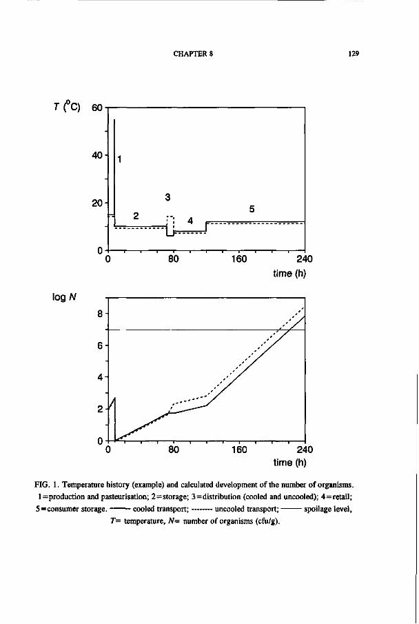
CHAPTER 8 129
7(°C) 60
time (h)
log/V
240 time (h)
FIG. 1. Temperature history (example) and calculated development of the number of organisms.
l=production and pasteurisation; 2=storage; 3=distribution (cooled and uncooled); 4=retail;
5=consumer storage. cooled transport; uncooled transport; spoilage level,
T= temperature, N= number of organisms (cfu/g).

130 CONCLUSIONS
Ln(/V//Vo) 18.2°C
0 40 80 120 160
(h1) 1.2
0.8
0.4
jU A
'
y
l time (h]
A \
Y
"0 10 20 30 40 50
V/i
T(°C)
= b(T-Tmit)V-exp[c(T-Tmax)]}
1
In N = / l exp {-exp [ ̂ 0 - 0 + 1 ] }
FIG. 2. Pathway of model building for bacterial growth as function of temperature (ji = specific
growth rate (h1), A = asymptotic level, \ = lag time (h), N = Number of organisms (cfu/ml),
N0 = number at time zero, e=exp(l), t = time (h), b, c, Tmiri, Tnax are Ratkowsky parameters).

CHAPTER 8 131
To describe the effect of physical and chemical conditions on deterioration, many
models are already proposed and many new ones can be generated. Selection procedures are
therefore needed. It is difficult to discriminate between models. Some advantages and
disadvantages of different modeling techniques will be presented.
Polynomial models: Polynomial models have the advantage that they are easy to use
(linear regression can be used), very straightforward and no knowledge is needed of the
process that is described. The disadvantages are: they do not contribute to knowledge about
the mechanisms underlying the process, they often have numerous parameters, because of the
numerous terms they can become unclear, problems can be encountered by fitting data that
disagree totally with the chosen polynomial function, and they are valid simply and solely
within the range of variables of the underlying measurements.
Empirical models: Empirical models (other than polynomials) have the advantage that
they can describe any curvature, and often need only few parameters. They do not contribute
much to insight, although often more so than polynomial models. Also these models can be
used only in a limited interval.
Mechanistic models: Mechanistic models have the advantage that they may increase the
insight into the process. They often can be combined more easily with other mechanistic
models. On the other hand, they often contain a large number of parameters and also are
applicable within a limited range. Often the model does not exactly describe what is
happening and discrepancies are tolerated, to keep the advantages of the mechanistic model.
In an Arrhenius plot, for instance, it is not unusual for the data to deviate from linearity in
one or more temperature regions [The Arrhenius model (1) was given a fundamental basis by
Eyring (4, 5)].
Use of models. In this thesis it has been shown that several descriptions of the effect of
temperature can be used to predict the growth of Lactobacillus plantarum. The temperature
is often one of the main variables that determine deterioration kinetics. To get a first
quantification of the development of the microbial numbers in a chilled product, several
growth curves of the main spoiler(s) have to be measured at different temperatures. The
growth parameters can be estimated from the resulting bacterial numbers using the modified
Gompertz equation (see Chapter 2). Firstly the effect of temperature (at suboptimum
temperatures) on the maximum specific growth rate can be described by the square-root
equation of Ratkowsky (11):
^ ; = ö ( 7 - 7 m i n ) a )

132 CONCLUSIONS
With linear regression, the parameters b and TmiB can be estimated. At different
temperatures the maximum specific growth rate can be calculated from these parameters. If
it is assumed that the bacteria are adapted to the environment (no lag time), that substrate
levels are sufficient, that metabolic product concentrations are not relevant, and that the initial
spoilage level ( N 0 ) is known, then exponential growth can be assumed and the number of
bacteria in time can be calculated from:
A/(0 = N„exp (n m - t ) (2)
With the parameters determined from these experiments we can calculate the microbial
quality at different temperatures, at any time during storage. Also the shelf-life ( 6 ) can be
calculated at different temperatures, if the maximum allowed spoilage level ( N e ) is known:
v °' (3) b 2 - ( 7 - - T m i n r
It is shown in Chapter 6 that in most cases the effect of temperature steps can be
neglected (immediate change of growth rate at a change of temperature) and that the
exponential growth, preceded by an eventual lag phase gives a reasonable prediction of the
development of the microorganisms. The above mentioned procedure can already give
valuable results concerning the progression of deterioration.
An example. As stated, a large amount of experimental data is essential to build and
validate models. As soon as a model is assumed to be correct it can be used with a much
smaller amount of experimental data. If, for instance, a chilled salad is mainly spoiled by
Lactobacillus, the growth rate of these bacteria is of importance. If the product should remain
unchanged, i.e. pH, water content, antimicrobial agents etc. are fixed, the temperature is the
variable left to control the spoilage. If equation 1 is used and the growth rate of Lactobacillus
at three temperatures (say 15°C, 20°C, and 25°C) is measured, the parameters Tmjn and b can
be calculated by linear regression, resulting in the following equation for the data given in
Table 1:
^ = 0 . 0 3 ( 7 - 5 . 2 5 ) (4)

CHAPTER 8 133
The data and the regression line are given in Fig. 3. If we assume exponential growth
we get:
ln[ jj- ) = 0 . 0 0 0 9 ( 7 - 5 . 2 5 ) 2 - 1 (5)
TABLE 1. Growth of lactobacilli in a salad (example)
T nm (h-')
(°C) (measured)
15 0.092
20 0.177
25 0.364
Regression
parameters
*=0.030
7^=5.25
nm (h-1)
(predicted)
0.086
0.196
0.351
VF (h ) 0.8
Tit)
FIG. 3. Ratkowsky plot of the specific growth rate of Lactobacillus in a salad (with 90% confidence interval).
With these three experiments equation 5 gives the microbial load at any desired
temperature between 15°C and 25°C, at any time during storage, if the initial spoilage level
is known. There is also some confidence that the model can be extrapolated to cover a larger
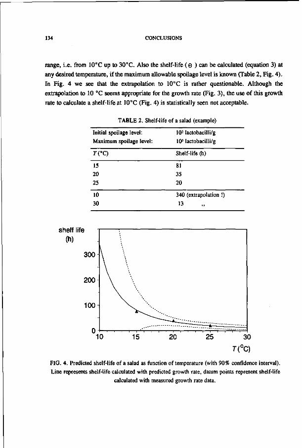
134 CONCLUSIONS
range, i.e. from 10°C up to 30°C. Also the shelf-life ( e ) can be calculated (equation 3) at
any desired temperature, if the maximum allowable spoilage level is known (Table 2, Fig. 4).
In Fig. 4 we see that the extrapolation to 10°C is rather questionable. Although the
extrapolation to 10 °C seems appropriate for the growth rate (Fig. 3), the use of this growth
rate to calculate a shelf-life at 10°C (Fig. 4) is statistically seen not acceptable.
TABLE 2. Shelf-life of a salad (example)
Initial spoilage level: Maximum spoilage level:
r(°C)
15 20
25
10
30
102 lactobacilli/g 105 lactobacilli/g
Shelf-life (h)
81 35 20
340 (extrapolation !)
13
shelf life (h)
300
200
100
FIG. 4. Predicted shelf-life of a salad as function of temperature (with 90% confidence interval). Line represents shelf-life calculated with predicted growth rate, datum points represent shelf-life
calculated with measured growth rate data.

CHAPTER 8 135
As shown, we can get preliminary insight from only a few experiments, once we have
a good model. Effects of temperature and initial spoilage level can be examined. It should be
noted, however, that more datum points give more accurate parameter values (with smaller
confidence intervals) and thus more accurate predictions. Furthermore, for every case
appropriate assumptions must be made.
The square-root relation (equation 1) is validated on par-fried fries and on chicken.
Specific growth rates at different temperatures are taken from literature data and from own
unpublished data. These measurements were all at suboptimum temperatures, therefore the
square-root relation can be used. The square-root of the specific growth rate is plotted versus
temperature, and the data are very well described by a straight line (Fig. 5 and 6). The fact
that the specific growth rates of both Wieringa and Viering (13) and Michener et al. (8) match
very well is very promising for the use of predictive models, since they were obtained in
studies using Dutch and American potatoes, in different laboratories (Fig. 5). Furthermore,
the total aerobic count is used, and the linear behaviour over a considerable range of
temperatures shows that there is no change resulting in a new flora with a totally different
kinetic behaviour. Also, the data on chicken (Fig. 6) agree very well. The data of Regez et
al. (12) were aerobic counts on chicken skin, our own unpublished data are Pseudomonas on
chicken skin, and the data of Pooni and Mead (9) and Barnes (2, 3) were Pseudomonas in
Heart Infusion Broth. These data from different laboratories, with different strains, on
different media all agree. The Ratkowsky parameters of these curves are given in Table 3.
TABLE 3. Rat
Fries
Chicken
cowsky parameters
b (°C-'h05)
0.0215
0.0301
on fries and chicken
T • CC) mm >• '
-7.36
-6.04
The main spoilage organism on both products was Pseudomonas spp, and both
parameter sets are of comparable order of magnitude. These examples demonstrate that with
relatively few experiments, or even with literature data only, a simple model can be
constructed which can be used for (preliminary) shelf-life prediction and optimization.
If the spoilage level of chicken is 5 107 (c.f.u./g) and the initial contamination after
production is 103 (c.f.u./g) and the storage temperature is 0°C, the shelf-life can be calculated
with equation 3 to be 14 days. In the distribution chain, it is difficult to maintain a temperature
of 0°C. If a producer has control over the distribution during the first 5 days and keeps the
temperature at 0°C, the number of bacteria can be calculated with equation 2 to increase to
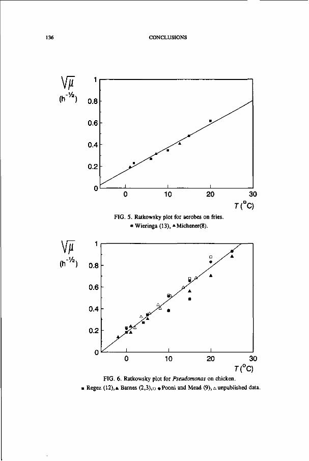
136 CONCLUSIONS
W 1
FIG. 5. Ratkowsky plot for aerobes on fries.
• Wieringa (13), * Michener(8).
FIG. 6. Ratkowsky plot for Pseudomonas on chicken.
Regez (12), A Barnes (2,3),a «Pooni and Mead (9), A unpublished data.

CHAPTER 8 137
5 104. If the product is then kept at 4°C (e.g., during retail display) the remaining shelf-life
can be calculated to be 3 days. So the total shelf-life is reduced from 14 days to 8 days and
the shelf-life during retail display is reduced from 9 days to 3 days. This can also be shown
graphically (Fig. 7). This kind of calculations can be used to show the importance of
supercooling to all parties participating in the food chain.
log(W) 12
15 20 time (days)
FIG. 7. Spoilage of chicken at 0°C and 5 days at 0°C and the remainder at 4°C ( 0°C; 5 days 0°C, then 4°C; spoilage level); N in c.f.u./g).
EXPANSION OF THE MODELS
These simple models can be expanded in several ways (resulting in more complex equations):
Incorporate a lag time and asymptote (See Chapters 4, 5 and 6).
Use of a sigmoidal growth curve for the predictions (see Chapters 2 and 6).
Use of the expanded square-root equation (necessary if also temperatures around or
above the optimum temperature are of importance) (Chapter 4).
Incorporate the effect of heat transport (see Heat Transport, below).
Incorporate logistics (operations research) (see Logistics, below).
Include other quality reactions, for instance chemical or physical (see Other
Deterioration Reactions, below).

138 CONCLUSIONS
Logistics. From the process variables in food production and distribution (e.g.,
temperature), the growth parameters ( A , [im, X.) of the organisms can be predicted (see Fig.
8). With these growth parameters the number of organisms with time can be predicted, and
feedback can follow, resulting eventually in adjustments in production or distribution (e.g.,
the temperature during distribution). This cycle of prediction and feedback can be repeated
many times.
Logistics Expert system
Production Distribution
N
7\pH, aw , r
\
M A a
FIG. 8. Optimization cycle of bacterial numbers.
It can also be worthwhile to incorporate logistics into this procedure, so that not only
the effect of changes in physical parameters of the process (e.g., temperature during
distribution) can be evaluated, but also the effect of changes in duration of the different stages
(e.g., duration of processing, holding, transportation, storage, break-down, or switch time).
Furthermore, the effect of distributions in several variables can be evaluated, such as
distributions in raw-material contamination, storage time in the retail display, temperature,
etc.
A preliminary program is developed to calculate costs of cooling in different stages of
a cooling chain. The optimum temperatures in a cooling chain can be calculated, combining
the square-root model and the maximum allowed bacterial number in a product. Three steps
in the distribution chain of milk are chosen as an example (factory storage, distribution,
supermarket storage). An overview of the most important contributions to energy costs is

CHAPTER 8 139
made. The most important contributions to energy costs for cooling are found to be the losses
through wall, floor, and roof; losses by opening of the door; and heat to be removed from the
product to reach the desired temperature.
With dynamic programming (backwards dynamic programming with fixed grid-points)
the optimum temperatures in the three phases are determined, with minimal costs, given a
certain quality. This procedure can be used for short term decisions. At present research on
this subject is in progress.
Management Tool. The quality functions given in this thesis can also be used for
long-term strategic decisions. For instance, the effect of an extra distribution centre, more
trucks for transportation, machinery with a lower technical failure chance etc. can be
evaluated. For these strategic decisions quality models are essential.
Other deterioration reactions. For other deterioration reactions (chemical, physical)
the same procedure can be followed. For chemical spoilage reactions, theory and application
are illustrated by Labuza (7). The progression of chemical and physical spoilage indicators
can be calculated simultaneously with the bacterial numbers, as a function of the physical
parameters. In this manner it can be evaluated which quality reaction determines the
shelf-life.
Knowledge-based system. As can be expected, all these procedures require a large
number of parameter values, such as the growth parameters of bacteria in different foods,
depending on different physical parameters, and the physical parameters of the different
foods. Therefore a large number of datum points must be collected and a large number of
experiments must be carried out, which can be collected in a database (Fig. 8). For practical
purposes it is impossible to have a database with all necessary information; therefore, it could
be useful to incorporate some knowledge into the database.
A combination of quantitative and qualitative data is of large importance, since there is
already a large quantity of these data. A start is made to develop a method to combine
qualitative and quantitative information. If this is done in a structured manner the method can
be used to predict product quality in the best possible way, given a limited amount of
information. This has been shown to result in a powerful tool to predict possible microbial
growth in different foods (see Chapter 7).

140 CONCLUSIONS
Residence Time Distribution. Growth models of microorganisms can be coupled to
residence time distributions (RTD) and computational fluid dynamics (CFD) programs to
calculate the effect of fluid flow in, for example, storage tanks or pipes. The effect of
residence time distribution and stagnant zones can be evaluated. In parts were the product will
stay long(er), more growth can occur, and due to mixing with the main stream a continuous
contamination occurs.
Heat transport. The above-mentioned square-root model for the temperature
dependency of [i m can be combined with a model for heat conductance in a product. This
will be explained by some examples. For the case that heat production can be neglected,
Fourier's second law for an infinite slab with thickness 2L, surrounded by fluid of
temperature Tf at both sides gives:
dJ _ d2T (6)
with a the thermal diffusivity (m2 s1), T the temperature (K), t the time (s), x the
location (m).
The boundary conditions are:
1) Due to the symmetry in the centre:
>-±) -o (7)
2) Since the transport through the surface of the slab is equal to the heat transport from the
fluid to the slab:
,dT\ (8)
with a the external heat transfer coefficient (Wm-'K1), and k the thermal conductivity
(W m1 K1). Equation 6 can be solved numerically by using difference equations.

CHAPTER 8 141
100 120
time (h)
log (A/)
100 120 time (h)
FIG. 9. Temperature history and development of the number of Lactobacillus. Simulation 1.
centre; intermediate position; surface , T= temperature,
N= number of organisms (cfu/g).

142 CONCLUSIONS
7(°C) 18
20 40 60 80 100 120
time (h)
log (A/)
100 120
time (h)
FIG. 10. Temperature history and development of the number of Lactobacillus. Simulation 2.
centre; intermediate position; surface, T= temperature,
N= number of organisms (cfu/g).

CHAPTER 8 143
In the program that is developed several successive phases can be entered (e.g., storage
raw-materials, production, cooling, product storage), with the temperature of the fluid in that
phase, as can the product characteristics. The set of equations then can be solved for every
time step and the temperature is calculated as a function of the location inside the product,
and as a function of time. Subsequently, the bacterial growth can be calculated, with the
square-root model, at any time at any point in the product. In this manner the effect of heating
and cooling of the product on the bacterial growth can be evaluated.
An example of a simulation is given below. A product is stored during 24 hours at
10°C, and then enters the 20°C production. The product stays there for 2 hours. After
production the product is stored in a cooling cabin with ventilation at 10°C (Table 4, Fig. 9).
It is assumed that the organisms are already in their exponential phase (lag time = 0).
For simulation 2 everything is the same as in simulation 1 except that during cooling
the product is cooled with 5 product units together, therefore the characteristic radius R is
increased by a factor 5 (Fig. 10).
In Fig. 9 and 10 the calculated temperature and the number of microorganisms are given
at three different locations in the product; the surface, the centre and in between (intermediate
position). In Fig. 9 it can be seen that the fastest temperature increase occurs at the surface
of the product, and about 17°C is reached. In the centre of the product and in the intermediate
position the heat equalisation goes slower. The effect of the higher temperature during
production on the number of micro-organisms is very small, due to the short time span.
TABLE 4. Parameters for Simulation 1
Time(h) Phase ro(°C) T,CC)
Process
Product
0-24 storage
24-26 production
26-100 cooling
infinite slab
characteristic radius
thermal diffusivity
thermal conductivity
10 10
10 20 a = 25 (Wm-2K')
20 10 a = 400 (convection)
R=0.05 m
a = 0.143 10-« (m2s>)
k= 0.60 (W m1 K-i)
Organism L. plantarum: JV„= 100 fc=0.0385 rmin=3.29 c=0.247 riMX=44.8
T0= product temperature when product enters phase, Tf= temperature of fluid in phase.

144 CONCLUSIONS
If the characteristic radius is increased by a factor 5 during cooling (Fig. 10), by joining
5 product units together, the cooling-down goes 25 times slower (proportional to the square
of the radius). The cooling-down of the middle and in the intermediate position of the slab
goes dramatically slower, which strongly facilitates bacterial growth at these positions. In
products with surface contamination only, this will be no real problem; in products with an
interior contamination, however, this can result in a serious problem.
Also the growth of an additional organism can be calculated, for instance Pseudomonas
spp, which is more psychrophilic than Lactobacillus. In simulation 3 everything is the same
as in simulation 1 except that the growth of Pseudomonas spp. (Table 5) is calculated as is
the growth of L. plantarum.
TABLE 5. Parameters for Pseudomonas spp
Pseudomonas spp.: No=10 *=003 rmin=-6.0 0=0.157 7^=36.0
In Fig. 11 the growth of Lactobacillus (7Vo=100) and Pseudomonas (No=l0) is
compared. Although the initial contamination is lower, the psychrophilic organisms will be
the main spoiling organisms.
log (A/)
100 120
time (h)
FIG. 11. Development of the number of Lactobacillus ( ) and Pseudomonas (-on the surface. Simulation 3. N= number of organisms (cfu/g).

CHAPTER 8 145
With comparable simulations the effects of numerous changes in production, product,
etc. can be evaluated. This can be an important tool for process optimization. The growth of
different organisms can be calculated by changing the growth parameters, as can the effect of
a change in initial contamination. Furthermore, the effect of different time/temperature
histories can be examined, as can the effect of different heating and cooling procedures
(forced convection, steam vs. water or air, different characteristic radii).
FESTAL CONCLUSION
Predictive modeling has shown to be a promising tool in food research, to be used to
optimize food chains. Various models are developed and validated to be used to describe
deterioration reactions.
A tool is developed to discriminate between different models and to restrict the number
of parameters in models. Models to describe a growth curve and to describe the effect of
temperature, and the effect of shifts in temperatures, are developed and validated with a large
amount of experimental data.
Furthermore, a procedure is developed to couple quantitative and qualitative
information in a structured manner. Simple procedures to make (preliminary) shelf-life
predictions are given, as are procedures to extend these (simple) models.
The most important advantage of modeling is that insight is gained in the progression
of microbial growth within a product chain. Furthermore, these models are shown to be
essential to calculate quality changes with the use of decision support systems (DSS).
REFERENCES
1. Arrhenius, S. 1889. Über die Reaktionsgeschwindigkeit bei der Inversion von Rohrzucker
durch Säuren. Z. Phys. Chem. 4:226-248.
2. Barnes E.M. 1976. Microbiological problems of poultry at refrigerator temperatures - a
review. J. Sei. Food Agric. 27:777-782.
3. Barnes E.M., G.C. Mead, C.S. Impey, and B.W. Adams. 1979. Spoilage organisms of
refrigerated poultry meat, p. 101-116. In Russell A.D. (ed.), Cold tolerant microbes in spoilage
and the environment. Academic Press, London.
4. Eyring, H. 1935. The activated complex in chemical reactions. J. Chem. Phys. 3:107-115.
5. Eyring, H., and J.L. Magee. 1942. Application of the theory of absolute reaction rates to
bacterial luminescence. J. Cell. Comp. Physiol. 20:169-177.

146 CONCLUSIONS
6. Gompertz, B. 182S. On the nature of the function expressive of the law of human mortality
and a new mode of determining the value of life contingencies. Philos. Trans. R. Soc. London
115:513-585.
7. Labuza T.P. 1985. An integrated approach to food chemistry: Illustrative cases. In O.R.
Fennema (ed.), Food Chemistry. Marcel Dekker Inc., New York.
8. Michener H.D., F.P. Boyle, G.K. Notter, and D.G. Guadagni. 1968. Microbiological
deterioration of frozen par-fried potatoes upon holding after thawing. Appl. Microbiol.
15:759-761.
9. Pooni G.S., and G.C. Mead. 1984. Prospective use of temperature function integration for
predicting the shelf-life of non-frozen poultry-meat products. Food Microbiol. 1:67-78.
10. Ratkowsky, D.A., R.K. Lowry, T.A. McMeekin, A.N. Stokes, and R.E. Chandler. 1983.
Model for bacterial culture growth rate throughout the entire biokinetic temperature range. J.
Bacteriol. 154:1222-1226.
11. Ratkowsky, D.A., J. Olley, T.A. McMeekin, and A. Ball. 1982. Relationship between
temperature and growth rate of bacterial cultures. J. Bacteriol. 149:1-5.
12. Regez P., L. Gallo, R.E. Schmitt, and W. Schmidt-Lorenz. 1988. Microbial spoilage of
refrigerated fresh broilers. Ill Effect of storage on the microbial association of poultry
carcasses. Lebensmittel Wiss. Technol. 21: 229-233.
13. Wieringa G.W., and J. Viering. 1973. Growth rate of microbes in par-fried french fries.
Mitteilungen IBVL (Institute for Storage and Processing of Agricultural Produce), Wageningen
8: 6 p.

147
SUMMARY
Growth of spoilage microorganisms in foods receives much attention since there is a
trend towards minimally processed foods. In these products growth of microorganisms is
possible. Therefore it is useful to know how fast microorganisms grow and which factors
determine this growth.
In this thesis different models are described to predict deterioration reactions. Models
are simplified descriptions of reality. By making appropriate assumptions, reality can be
described with mathematical relations. With these mathematical equations predictions can be
made of the progress of a process. This can give insight in these kinetics. These equations can
also be used to optimize processes.
Various factors determine the growth of microorganisms like temperature, pH, water
activity, gas-atmosphere and the presence of preservatives. Some of these factors not only
influence the growth rate of microorganisms but also the properties of the product (pH, water
activity, salt concentration, preservatives). A change in storage temperature or
gas-atmosphere (within certain limits) only changes the growth rate of the microorganisms.
With these two factors it is possible to alter the spoilage rate of a product and thus the shelf
life, without changing the product. In this thesis mainly the effect of temperature is
investigated.
A tool to discriminate between different models is proposed, leading to restriction of
the number of parameters in the models applied. Models are developed to describe a bacterial
growth curve. Furthermore, models are developed to describe the effect of temperature, and
the effect of shifts in temperature. These models are validated with a large number of
experimental data. Simple procedures to make shelf life predictions with these models are
given, as are procedures to extend these models.
In order to make shelf-life predictions of products with varying composition, several
parameters are needed. For some of these, quantitative information is available, for others
only qualitative. Therefore, a procedure is developed to couple quantitative and qualitative
information in a structured manner. In this manner an estimate of the shelf life can be made
on the basis of parameter values combined with qualitative information, in order to get a
prediction as good as possible, on basis of available knowledge.

148
The most important advantage of modeling is that insight is gained in the kinetics of
microbial growth within a product chain. Furthermore, these models are essential to calculate
quality changes in decision support systems (DSS).
149
SAMENVATTING
Groei van bederfveroorzakende micro-organismen in levensmiddelen staat sterk in de
belangstelling, aangezien veel produkten momenteel minder conserveringsbewerkingen
ondergaan dan voorheen. Door het geheel of gedeeltelijk ontbreken van deze bewerkingen
(zoals bijvoorbeeld sterilisatie, zouten, het gebruik van conserveermiddelen), wordt groei van
micro-organismen begunstigd. Het is dan nuttig te weten hoe snel de micro-organismen
groeien en welke factoren die groei beïnvloeden.
In dit proefschrift worden verschillende modellen beschreven, die microbiologische
bederfreacties kunnen beschrijven. Modellen zijn vereenvoudigde voorstellingen van de
werkelijkheid. Door geschikt gekozen veronderstellingen te doen kan de werkelijkheid
beschreven worden met wiskundige relaties. Met deze wiskundige relaties kunnen dan
voorspellingen gedaan worden over het verloop van bepaalde processen. Hierdoor kan inzicht
verkregen worden in de kinetiek van die processen. Deze relaties kunnen ook gebruikt
worden om processen te optimaliseren.
Verschillende factoren zijn van invloed op de groei van micro-organismen, zoals de
temperatuur, de pH, de wateractiviteit, de gasatmosfeer en de aanwezigheid van
groeiremmende stoffen. Sommige van deze factoren veranderen behalve de groeisnelheid van
de micro-organismen echter ook de aard van het produkt (pH, wateractiviteit,
zoutconcentratie, conserveringsmiddelen). Verandering van de bewaartemperatuur of de
gasatmosfeer (binnen bepaalde grenzen) verandert alleen de groeisnelheid van de
micro-organismen. Bij een gegeven produktsamenstelling is het dus mogelijk de
bederfsnelheid en daarmee de houdbaarheid te beïnvloeden, zonder het produkt te
veranderen. In dit proefschrift is voornamelijk onderzoek verricht naar het effect van de
temperatuur.
Er is een methode opgesteld om tussen verschillende modellen te discrimineren om zo
het aantal parameters in de modellen te minimaliseren. Allereerst zijn er modellen ontwikkeld
om een groeicurve van micro-organismen te beschrijven. Verder zijn er modellen ontwikkeld
om het effect van de temperatuur en het effect van temperatuurstappen te voorspellen. Deze
modellen zijn getoetst met een groot aantal experimentele gegevens. Eenvoudige procedures
om houdbaarheidsvoorspellingen te doen worden gegeven, evenals procedures om deze
modellen uit te breiden.

150
Om houdbaarheidsvoorspellingen te kunnen doen van allerlei produkten met
verschillende samenstelling zijn verschillende parameters nodig. Over enkele hiervan is
kwantitatieve kennis beschikbaar, over andere slechts kwalitatieve. Daarom is er een
procedure ontwikkeld om kwantitatieve en kwalitatieve gegevens op een gestructureerde
manier te koppelen. Op deze manier kan de best haalbare schatting van de houdbaarheid
gemaakt worden op basis van parameterwaarden gekoppeld aan kwalitatieve kennis.
Het grootste voordeel van modelleren is dat inzicht kan worden verkregen in de kinetiek
van de groei van micro-organismen in produktketens. Verder zijn deze modellen essentieel
om kwaliteitsveranderingen te berekenen in beslissings-ondersteunende systemen (BOS).

151
NAWOORD
Het in dit proefschrift beschreven onderzoek is tot stand gekomen dankzij de hulp en
inzet van een groot aantal personen, waarvan ik er hier enkele wil bedanken.
In de eerste plaats wil ik Klaas van 't Riet noemen. Klaas, die een goede manager is,
maar toch meer een vriend dan een meerdere, is een ideale baas. Frans Rombouts en Jacora
de Wit hebben mij op zeer vriendelijke wijze een aantal aspecten van de
levensmiddelenmicrobiologie bijgebracht. Verder hebben ze mij bijgestaan in raad en daad
bij het schrijven van publikaties. Rik Beeftink, die een gezellige en stimulerende kamergenoot
was, heeft hier ook zijn steentje aan bijgedragen. Rhea Rekker wil ik bedanken voor de hulp
bij het ontwerp van de omslag en het commentaar op de lay-out. Paul Verlaan wil ik bedanken
voor het aanzwengelen van dit onderzoek en voor zijn begeleiding in de beginfase.
Binnen het kader van dit onderzoek heeft een tweetal analisten een grote hoeveelheid
werk verzet, te weten Birgit Hasenack en Ida Günther. Verder heeft een groot aantal
studenten een bijdrage geleverd aan het onderzoek in de vorm van een afstudeervak bij
Proceskunde of Levensmiddelenmicrobiologie, te weten: Jolanda de Koos, Ida Jongenburger,
Monique Mellema, Lucas Ledelay, Jaap Roosma, Jolanda Zondag, Carin Groen, John van
den Broek, Liesbeth Oosterom, Chusnul Hidayat, Taco Wijtzes, Onno de Waart, Erwin Kaal,
Liesbeth Elbertsen, Brigitte Campfens, Nanette Koers, Noor van Hapert en Rob Verhagen.
Het project is mede gefinancierd door het Unilever Research Laboratorium
Vlaardingen. Piet Klapwijk, Jan Smelt, Henk Cuppers, en Pieter ter Steeg wil ik bedanken
voor hun nuttige inbreng bij de wederzijdse bezoeken.
De medewerkers van de werkplaats, fotolocatie, tekenkamer, afdeling automatisering,
en de magazijnen van de Centrale Dienst Biotechnion wil ik bedanken voor hun verrichte
diensten.
Als laatste maar zeker niet als onbelangrijkste wil ik de gehele sectie proceskunde
bedanken. Het is een prima groep om in te werken, ik denk niet dat er veel plaatsten zijn waar
je op zo een prettige wijze met je collega's om kunt gaan.

152
CURRICULUM VITAE
Marcel Zwietering werd op 10 augustus 1963 geboren in Sittard. In 1981 behaalde hij
het diploma VWO-B met lof aan de Serviam scholengemeenschap in Sittard. In datzelfde jaar
begon hij met zijn studie aan de toenmalige Landbouwhogeschool Wageningen.
In mei 1985 legde hij het kandidaatsexamen in de richting Moleculaire Wetenschappen
met lof af. In de doctoraalfase van deze studie deed hij de hoofdvakken Microbiologie en
Proceskunde en de bijvakken Wiskunde en Meet- Regel- en Systeemtechniek. Zijn
stage-periode bracht hij door bij het Department of Chemical Engineering, MIT, Cambridge,
USA, bij professor Cooney. In november 1987 studeerde hij met lof af. Hij werd in 1987
onderscheiden met een Unilever Research Prijs.
Van december 1987 tot en met december 1988 was hij als AIO verbonden aan de sectie
Proceskunde van de Landbouwuniversiteit Wageningen. Van januari 1989 tot heden is hij
werkzaam als universitair docent bij dezelfde sectie. Van december 1987 tot december 1992
verrichtte hij het onderzoek (mede gefinancierd door Unilever Research) dat leidde tot dit
proefschrift.