MODELING OF STATIC AND KINETIC FRICTION IN RUBBER...
37
MODELING OF STATIC AND KINETIC FRICTION IN RUBBER-PAD FORMING PROCESS by MAZIAR RAMEZANI Thesis submitted in fulfillment of the requirements for the degree of Doctor of Philosophy November 2009
Transcript of MODELING OF STATIC AND KINETIC FRICTION IN RUBBER...

MODELING OF STATIC AND KINETIC
FRICTION IN RUBBER-PAD FORMING
PROCESS
by
MAZIAR RAMEZANI
Thesis submitted in fulfillment of the requirements
for the degree of
Doctor of Philosophy
November 2009

ii
Acknowledgements
I would like to express my sincere gratitude to my supervisor, Assoc. Prof. Dr.
Zaidi Mohd Ripin for his continuing encouragement, intellectual discussions and
insightful suggestions. I benefited a lot from him both professionally and personally.
It is an honor to be his graduate student. I would also like to thank my co-supervisor,
Assoc. Prof. Dr. Roslan Ahmad for all the help.
My thanks are due to the technicians of School of Mechanical Engineering, who
have helped me in my experimental works.
I would like to thank my parents for their constant support and love. They inspired
and strengthened me emotionally, spiritually, and intellectually in every step of my
life.
Finally, I want to thank my wife for all the support. During my research activities,
her patience, understanding, encouragement and love helped me go through every
obstacle and make my life here enjoyable and productive.

iii
TABLE OF CONTENTS
Acknowledgements…………………………………………………...…………..ii
Table of contents…………………………………………………...…………….iii
List of tables…………………………………………………………...…………vi
List of figures……………………………………………………………………vii
Nomenclature…………………………………………………………….………x
Abstrak………………………………………………………………………..…xii
Abstract…………………………………………………………………………xiii
1. Introduction
1.1 Rubber-pad forming process…………………………...…………………1
1.2 Friction in rubber-pad forming process…………………………………..5
1.2.1 Static friction……………………………………..……………….6
1.2.2 Kinetic friction……………………………...…………………….8
1.3 Objectives ……………..…………………………………………..……10
1.4 Overview……………………………………………….………………..10
2. Literature review
2.1 Introduction………………………………………...……………………12
2.2 Rubber-pad forming process……………………………………….……12
2.3 Asperity contact models…………………………………………………13
2.4 Static friction in rubber/metal contact….………………………………..15
2.5 Kinetic friction in metal/metal contact………………………….………18
2.6 Conclusion……………...……………………………………….………20
3. Static and kinetic friction models for rubber-pad forming
3.1 Introduction…………………………………………….………………..21
3.2 Coulomb friction model…………………………………...…………….21

iv
3.3 Single-asperity static friction model for rubber/metal contact….………22
3.3.1 Normal loading of a viscoelastic/rigid asperity couple…….……25
3.3.2 Tangential loading of viscoelastic/rigid asperity couple…..……27
3.4 Multi-asperity static friction model for rubber/metal contact………..….29
3.4.1 Normal loading of viscoelastic/rigid multi-asperity contact…….31
3.4.2 Tangential loading of viscoelastic/rigid multi-asperity contact…32
3.5 Stribeck-type kinetic friction model for metal/metal contact………...…36
3.6 Conclusion…………………………………………………………....…43
4. Rubber-pad forming process; Experiments and finite element validation
4.1 Introduction…………………………..………………………………….45
4.2 Experimental set-up and finite element simulation……..………………45
4.3 Results and discussion ……………………………………………….…52
4.3.1 Forming stages……………………………………….………….52
4.3.2 In-plane maximum principal stress……………………...………53
4.3.3 Thickness distribution…………………………….……………..56
4.3.4 Load-stroke curves…………………………………...………….57
4.3.5 FE validation………………………………………………...…..58
4.3.6 Effect of rubber-pad thickness………………………………..…59
4.3.7 Effect of Coulomb coefficient of friction…………………….…61
4.3.8 Stress-strain analysis…………………………………………….62
4.4 Conclusions…………………………………………………………...…65
5. Results of static and kinetic friction models
5.1 Introduction………………………………………..…………………….67
5.2 Static friction results …………………………..………………………..67
5.3 Kinetic friction results…………………………………….……………..74

v
5.4 Effect of contact conditions on coefficient of friction…………………..78
5.5 Conclusions………………………………………………………….…..80
6. Conclusions and Recommendations
6.1 Conclusions…………………………………………………………...…82
6.2 Recommendations……………………………………………….………83
References……………………………………………………………...……….84
List of publications…………………………….……………………………….89

vi
LIST OF TABLES Page
Table 4.1 Ogden (N=3) constants for natural rubber 51
Table 4.2 Ogden (N=3) constants for silicon rubber 51
Table 5.1 Values of the input parameters for static friction model 70
Table 5.2 Values of the input parameters for kinetic friction model 75
vii
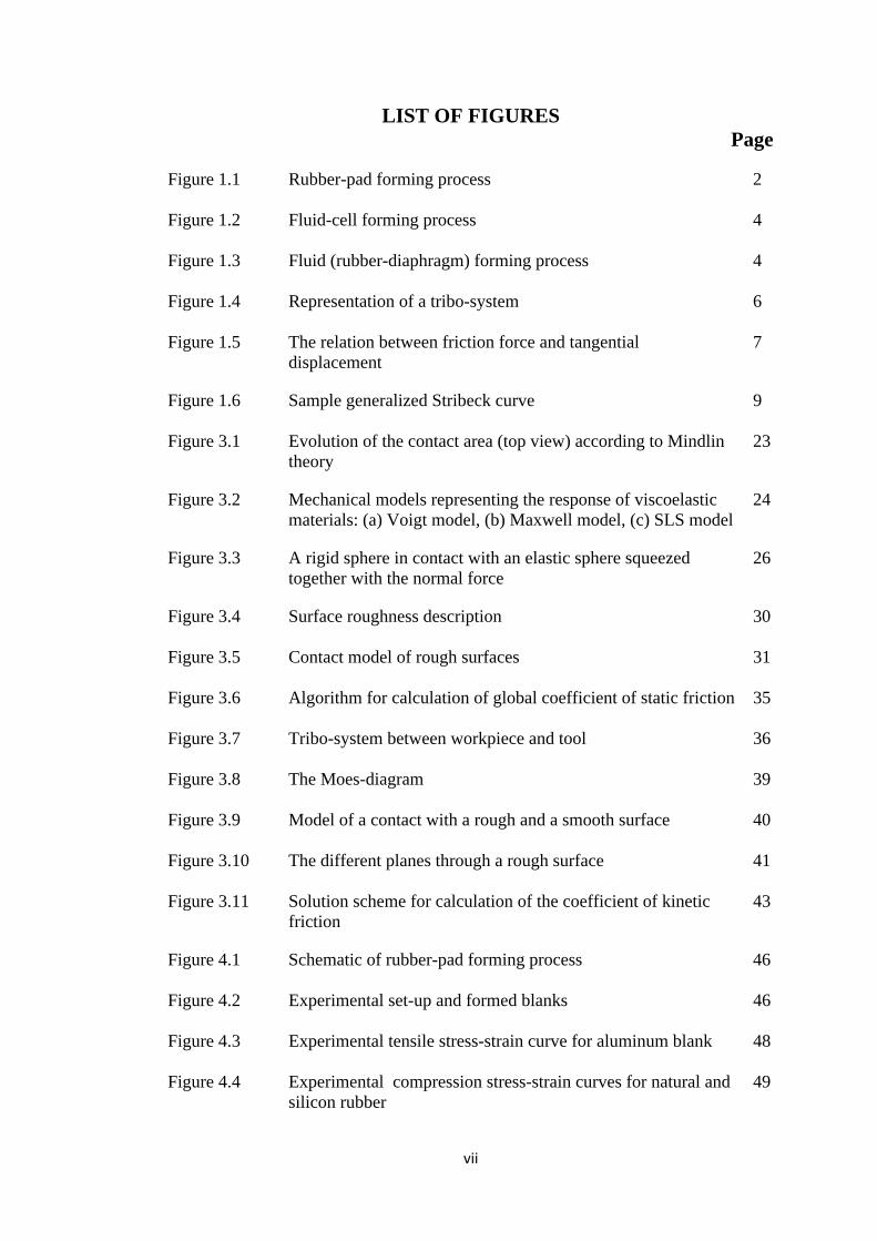
LIST OF FIGURES Page
Figure 1.1 Rubber-pad forming process 2
Figure 1.2 Fluid-cell forming process 4
Figure 1.3 Fluid (rubber-diaphragm) forming process 4
Figure 1.4 Representation of a tribo-system 6
Figure 1.5 The relation between friction force and tangential displacement
7
Figure 1.6 Sample generalized Stribeck curve 9
Figure 3.1 Evolution of the contact area (top view) according to Mindlin theory
23
Figure 3.2 Mechanical models representing the response of viscoelastic materials: (a) Voigt model, (b) Maxwell model, (c) SLS model
24
Figure 3.3 A rigid sphere in contact with an elastic sphere squeezed together with the normal force
26
Figure 3.4 Surface roughness description 30
Figure 3.5 Contact model of rough surfaces 31
Figure 3.6 Algorithm for calculation of global coefficient of static friction 35
Figure 3.7 Tribo-system between workpiece and tool 36
Figure 3.8 The Moes-diagram 39
Figure 3.9 Model of a contact with a rough and a smooth surface 40
Figure 3.10 The different planes through a rough surface 41
Figure 3.11 Solution scheme for calculation of the coefficient of kinetic friction
43
Figure 4.1 Schematic of rubber-pad forming process 46
Figure 4.2 Experimental set-up and formed blanks 46
Figure 4.3 Experimental tensile stress-strain curve for aluminum blank 48
Figure 4.4 Experimental compression stress-strain curves for natural and silicon rubber
49

viii
Figure 4.5 Comparison of Mooney-Rivlin and Ogden hyper-elastic models
51
Figure 4.6 Three stages of rubber-pad forming process 52
Figure 4.7(a) Specimen cross section after cutting measured by Alicona microscope
53
Figure 4.7(b) FE model of rubber-pad forming. The numbers labeled are the locations for thickness measurement
53
Figure 4.8 Symbol plots of in-plane maximum principal stress 55
Figure 4.9 Experimental thickness distribution of the formed part at 1min.5 −= mmV p
57
Figure 4.10 Experimental load-stroke curves using natural and silicon rubber as flexible punches
58
Figure 4.11 Comparison of experimental and FEM thinning results for specimen formed by natural rubber
59
Figure 4.12 Von-Mises stress distribution with different rubber-pad thicknesses
60
Figure 4.13 Thickness distribution of formed parts with different rubber-pad thicknesses
61
Figure 4.14 Thickness distribution of formed parts with different coefficients of friction
62
Figure 4.15 Stress distribution during rubber-pad forming simulation with natural rubber
64
Figure 4.16 Strain distribution during rubber-pad forming simulation with natural rubber
64
Figure 5.1 Asperity and valley distribution in the surface of natural rubber obtained from Alicona optical microscope
68
Figure 5.2 Roughness profile for natural rubber 68
Figure 5.3 Stress relaxation modulus as a function of time for natural rubber Shore A hardness 50
69
Figure 5.4 Coefficient of static friction (for natural rubber/AA6061-T4 contact) as a function of normal load
70
Figure 5.5 Punch load-stroke curve using different static friction models 73
Figure 5.6 Thickness distribution using different static friction models 73
ix
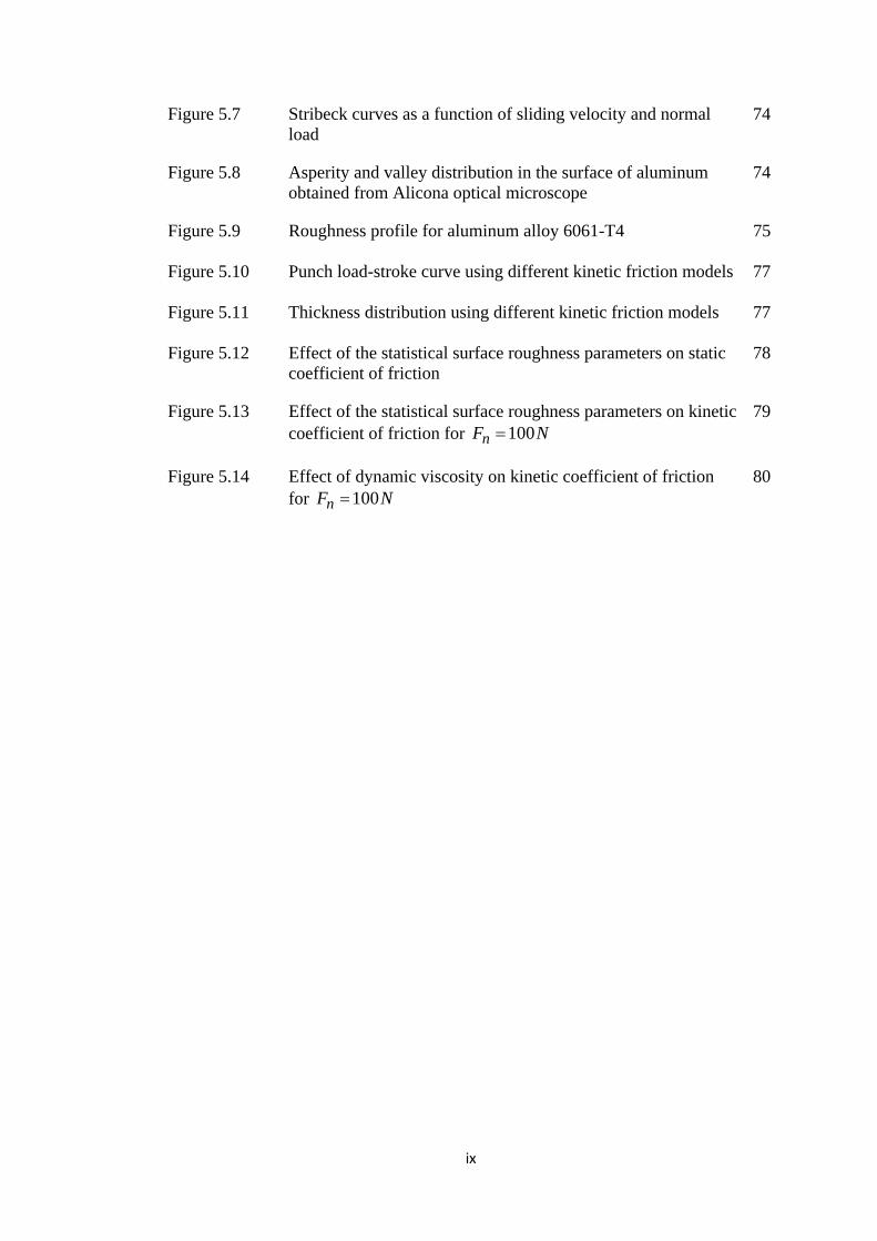
Figure 5.7 Stribeck curves as a function of sliding velocity and normal load
74
Figure 5.8 Asperity and valley distribution in the surface of aluminum obtained from Alicona optical microscope
74
Figure 5.9 Roughness profile for aluminum alloy 6061-T4 75
Figure 5.10 Punch load-stroke curve using different kinetic friction models 77
Figure 5.11 Thickness distribution using different kinetic friction models 77
Figure 5.12 Effect of the statistical surface roughness parameters on static coefficient of friction
78
Figure 5.13 Effect of the statistical surface roughness parameters on kinetic coefficient of friction for NFn 100=
79
Figure 5.14 Effect of dynamic viscosity on kinetic coefficient of friction for NFn 100=
80

x
NOMENCLATURE Roman symbols a contact radius, m
a′ half width of Hertzian contact, m
nA nominal contact area, 2m
rA real contact area, 2m
B contact length, m c radius of the stick zone, m
dd distance between mean line of asperity and mean line of surface, m
E Young’s modulus, Pa
E′ equivalent modulus of elasticity, Pa
fF sliding friction force, N
cfF , friction force from asperity interaction, N
hfF , hydrodynamic friction force, N
nF normal load, N
maxstF maximum static friction force, N
tF tangential load, N
g elasticity of the springs in SLS model, Pa
G shear modulus, Pa
h separation, m
ch lubricant film thickness, m
n density of asperities, 2−m p pressure, Pa
hP maximum Hertzian pressure, Pa
mP mean Hertzian pressure, Pa
R′ equivalent radius, m
s asperity height, m
t time, s
u sliding velocity, 1−ms z surface height, m

xi
Greek symbols
β mean radius of asperity, m
0β slope of the limiting shear stress-pressure relation, 0.047
η dynamic viscosity at zero pressure and Co40 temperature, sPa.
0η dynamic viscosity at ambient pressure, sPa.
dη viscosity of dashpot in SLS model, sPa.
τ shear stress, Pa
Lτ limiting shear stress, Pa
0Lτ limiting shear stress at ambient pressure, Pa
nδ normal approach, m
tδ tangential displacement, m
)(tϕ creep compliance function, 1−Pa
)(tψ stress relaxation function
μ local coefficient of friction
cμ Coulomb coefficient of friction
kμ kinetic coefficient of friction
sμ static coefficient of friction
ρ density, 3. −mkg
γ scaling factor
ν Poisson’s ratio
)(sθ normalized Gaussian height distribution
sσ standard deviation of the asperity heights, m
Abbreviations
BL Boundary Lubrication EHL Elasto-Hydrodynamic Lubrication FEM Finite Element Method ML Mixed Lubrication SMF Sheet Metal Forming

xii
MODEL GESERAN STATIK DAN KINETIK DI DALAM PROSES
PEMBENTUKAN BERLAPIK GETAH
ABSTRAK Keadaan geseran di dalam simulasi proses pembentukan kepingan logam biasanyna
dikira dengan menggunakan pekali geseran malar (model Coulumb). Tesis ini
membangunkan model geseran statik dan kinetik berasaskan keadaan sentuhan dan
mengambilkira kesan tekanan, halaju, kekasaran permukaan dan kelikatan pelincir
terhadap pekali geseran. Puncak-puncak pada permukaan dimodel secara statistik
dengan taburan Gauss dan puncak-puncak pada permukaan getah dianggap sebagai
elastik-likat. Pada permukaan bersentuh di antara acuan dan kepingan logam jumlah
daya di dalam arah normal di anggap di kongsi bersama oleh daya angkatan
hidrodinamik dan daya-daya saling tindak puncak-puncak pada permukaan. Model
geseran yang dibangunkan menunjukkan pada daya normal yang rendah, pekali
geseran mengurang dengan banyak apabila beban meningkat dan mencapai tahap
malar pada beban tinggi. Pekali geseran kinetik mengurang dengan pertambahan
halaju gelinciran dan daya arah normal. Secara teorinya dapat ditunjukkan pekali
geseran menjadi lebih besar bagi permukaan yang lebih kasar dan dengan pelincir
yang lebih likat, pekali geseran kinetik berkurangan. Sebagai tambahan ujikaji dan
simulasi pembentukan berlapik getah dilakukan. Lengkuk gesearan daripada
pengiraan menggunakan model geseran yang baru dilaksanakan di dalam kod unsur
terhingga ABAQUS/Standard. Keputusan simulasi menunjukkan model geseran
yang baru memberikan korrelasi yang lebih baik dengan keputusan ujikaji
berbanding menggunakan model Coulumb dari segi lengkuk beban hentam-lejang
dan ramalan penipisan. Ralat bagi ramalan kaedah unsur terhingga ialah 8% bagi
model geseran Coulumb dan 5.6% bagi model geseran kinetik. Ralat ini berkurangan
kepada 4.8% bila model geseran statik digunakan.
xiii
MODELING OF STATIC AND KINETIC FRICTION IN RUBBER-PAD
FORMING PROCESS
ABSTRACT
The frictional behaviour in sheet metal forming simulations is often taken into
account by using a constant coefficient of friction (Coulomb model). This thesis
develops static and kinetic friction models which are based on local contact
conditions and consider the effect of pressure, velocity, surface roughness and
lubricant viscosity on coefficient of friction. The surface asperities were modeled
using statistical Gaussian distribution and the behavior of rubber asperities was
assumed to be viscoelastic. In lubricated contact surface between die and sheet, the
total normal load was assumed to share by the hydrodynamic lifting force and the
asperity interacting force. According to developed friction models, at low normal
loads the static friction coefficient decreases sharply with increasing normal load and
reaches a quite stable level at higher loads. The coefficient of kinetic friction
decreases with increasing the sliding velocity and normal load. It was shown
theoretically that the coefficient of friction is larger for rougher surfaces, and by
increasing the lubricant viscosity, the coefficient of kinetic friction decreases.
Furthermore, rubber-pad forming experiments and simulations were performed. The
calculated friction curves using the new friction models were implemented in the
finite element code ABAQUS/Standard. From the results of simulations it was found
that the new friction models have better correlation with experimental results
compared to traditional Coulomb friction model, in terms of punch load-stroke curve
and thinning prediction. The FE prediction error for maximum punch load is 8%
using Coulomb friction model and 5.6% using the kinetic friction model. The error
decreases to 4.8% using the static friction model.
1
Chapter 1
Introduction
1.1 Rubber-pad forming process
All Sheet Metal Forming (SMF) processes have in common that they are mostly
performed with the aid of presses which drive the tools to deform the initially flat
sheet material into a product. The sliding of a plastically deforming sheet against the
tools makes both tribological as well as mechanical knowledge necessary for
optimum processing.
The conventional SMF process is performed through a rigid punch, which together
with a blank-holder, forces the sheet metal to slide into a die and comply with the
shape of the die itself. Rubber forming adopts a rubber pad contained in a rigid box
in which one of the tools (die or punch) is replaced by the rubber pad. The elastomer
incompressibility is exploited: deforming at constant volume, it exerts a hydrostatic
pressure on the sheet metal. Such a technology possesses several advantages: in this
process, only a single rigid tool half is required to form a part. One rubber pad takes
the place of many different die shapes, returning to its original shape when the
pressure is released. Tools can be made of low cost, easy-to-machine materials due to
the hydrostatic pressure exerted on the tools. The bending radii changes
progressively during forming process. Using rubber as flexible punch, thinning of the
workpiece, as occurs in conventional deep drawing, is reduced considerably. The
same tool set-up can be used to stamp different materials and different thicknesses.
Components with excellent surface finish can be formed as no tool marks are
created. The set-up time is reduced, because the punch-to-die alignment procedure is

2
no longer necessary. Lubrication is usually not needed. Disadvantages consist of the
short operating life of the rubber pads, lower stamping pressure which results in parts
with less sharpness that may require subsequent hand works and the production rate
is low. Rubber forming technology is particularly suited to the production of
prototypes and small series (Thiruvarudchelvan, 1993 and Sala, 2001).
Rubber forming can be divided into three main categories: i.e., rubber-pad forming,
fluid-cell forming and fluid forming. Among these techniques, rubber-pad forming
process (see, Figure 1.1) is the oldest and simplest, its advantages consisting of
tooling profitability and production flexibility, suited for small series. The rubber
pads in this method may be constructed either solidly or laminated. The laminated
pad comprised of sheets of rubber placed over one another. The advantage they have
is that the working surface can be restored by turning the top layer over or replacing
it. The rubber chamber and form block are made of steel or cast iron (able to sustain
forming pressures of 50-140 MPa) and the rubber pad is made of a soft (50-75 Shore
hardness) elastomer. Maximum stamping depth seldom exceeds 50 mm, which can
be increased by using thicker pads and more powerful presses (Sala, 2001).
Figure 1.1 Rubber-pad forming process (Sala, 2001).

3
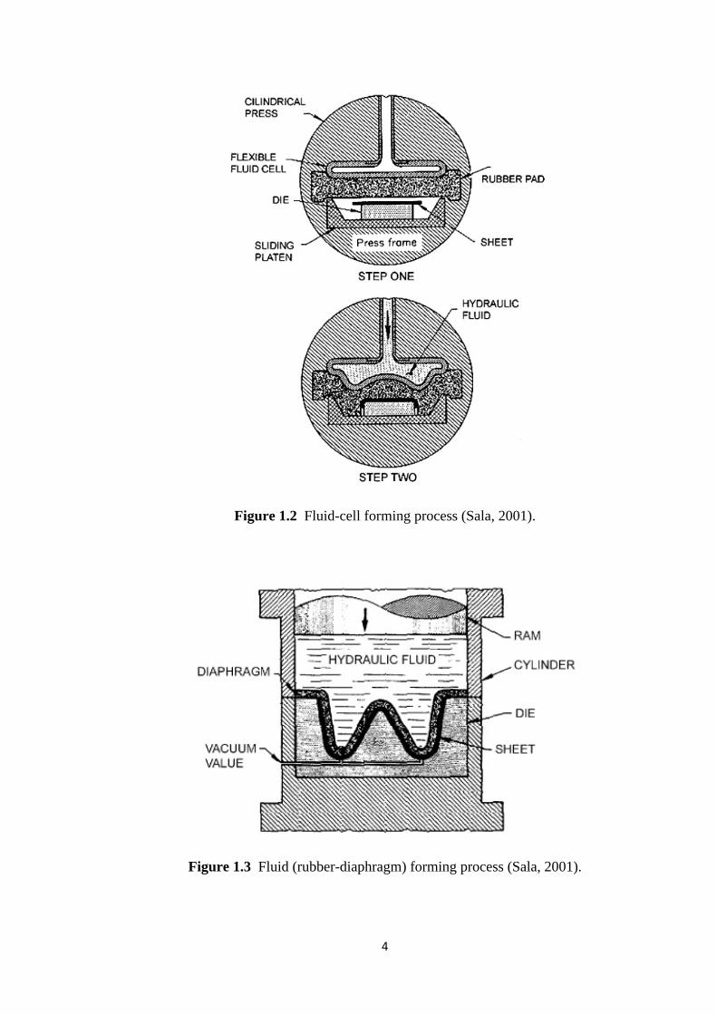
The methods belonging to fluid-cell forming category (see, e.g., Figure 1.2) use the
elastomer as a medium placed between sheet metal and a flexible container (fluid
cell) filled with a hydraulic fluid and able to apply a hydrostatic pressure to the
workpiece. These methods can produce deep (up to 400-450 mm), undercut and
intricate components. In the fluid-cell forming method shown in Figure 1.2, a pump
pressurizes a flexible fluid cell. The fluid cell wall is protected from the contact with
sheet metal by a soft rubber pad. Without punch movements, the fluid cell expansion
forces the rubber pad to comply to the die contour, thus exerting a hydrostatic
pressure on the sheet metal to take the shape of the die (Sala, 2001).
Fluid forming (or rubber-diaphragm forming) technologies (see, e.g., Figure 1.3)
also exploit flexible punch to prevent stress concentrations, they differ from rubber-
pad and fluid-cell forming processes because the forming pressure depends on the
forming depth. In the fluid forming method shown in Figure 1.3, a hydraulic fluid,
pressurized by an actuator forces the sheet metal against the die contour, while an
inlet valve removes trapped air; a rubber diaphragm shields the sheet metal and
distributes pressure.
Compared to fluid-cell forming and rubber-diaphragm forming, rubber-pad
forming has a further advantage that sealing problems and the possibility of leakage
of the high-pressure liquid are eliminated (Thiruvarudchelvan, 2002). Up to 60% of
all sheet metal parts in aircraft industry such as frames, seat parts, ribs, windows and
doors are fabricated using rubber-pad forming processes (Lascoe, 1988). In other
industries, for instance automotive industry, this process is mainly used for
prototypes or pilot productions. In this thesis, rubber-pad forming process is adopted
for analysis and experiments, because both static and kinetic friction regimes are
available simultaneously during this process.
4
Figure 1.2 Fluid-cell forming process (Sala, 2001).
Figure 1.3 Fluid (rubber-diaphragm) forming process (Sala, 2001).

5
1.2 Friction in rubber-pad forming process
“Tribology” is the science and technology of interacting surfaces in relative
motion. It is best studied by looking at the system of parameters influencing the
frictional behaviour of bodies in contact with each other. This means that not only
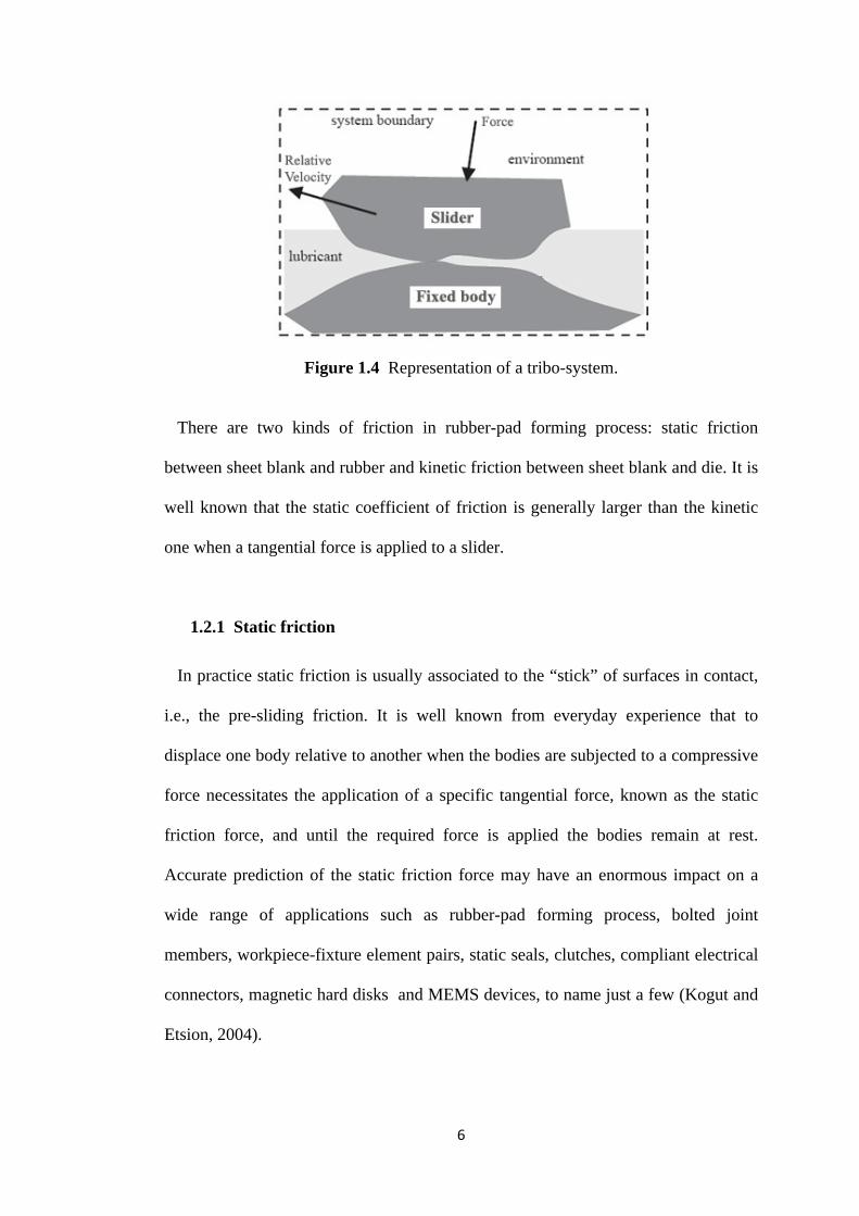
the contact itself is of importance but also that the environment of the contact plays a
role. A general tribo-system is shown in Figure 1.4. This system consists of the
following elements: two bodies which interact with each other, a lubricant and the
environment.
In recent years, the finite element method (FEM) has been widely used to simulate
SMF operations. The simulations are used for quality control and problem analysis
such as tearing, wrinkling and surface distortion. The usefulness of such analysis is
limited by the accuracy of the description of the friction phenomena in the sheet/tool
contact area (Lee et al., 2002). For SMF processes, the frictional behaviour depends
on several parameters such as the contact pressure, sliding speed, sheet and tool
material, surface roughness, lubricant and concurrent deformation (Wilson, 1979).
Especially when the blank thickness/blank area ratio is small, the friction influences
the material flow and with this the final strain distribution. Since all of these
variables influence friction, the question arises as whether the Coulomb simple
friction model is capable of describing the real frictional properties of sheet metal
forming processes. Some results have pointed out that a friction model based on local
contact conditions is more advantageous than the Coulomb friction model, especially
in a range of higher sliding velocities (see, e.g., Matuszak, 2000).
6
Figure 1.4 Representation of a tribo-system.
There are two kinds of friction in rubber-pad forming process: static friction
between sheet blank and rubber and kinetic friction between sheet blank and die. It is
well known that the static coefficient of friction is generally larger than the kinetic
one when a tangential force is applied to a slider.
1.2.1 Static friction
In practice static friction is usually associated to the “stick” of surfaces in contact,
i.e., the pre-sliding friction. It is well known from everyday experience that to
displace one body relative to another when the bodies are subjected to a compressive
force necessitates the application of a specific tangential force, known as the static
friction force, and until the required force is applied the bodies remain at rest.
Accurate prediction of the static friction force may have an enormous impact on a
wide range of applications such as rubber-pad forming process, bolted joint
members, workpiece-fixture element pairs, static seals, clutches, compliant electrical
connectors, magnetic hard disks and MEMS devices, to name just a few (Kogut and
Etsion, 2004).

7
Figure 1.5 The relation between friction force and tangential displacement.
In the static friction regime, the friction force increases with increasing tangential
displacement up to the value necessary to initiate macro-sliding of the bodies in
contact, as depicted in Figure 1.5. Although, the bodies are macroscopically in rest, a
micro-displacement occurs at the interface which precedes the macro-sliding
situation (Persson et al., 2003). This micro-displacement can reach relatively large
values when one of the surfaces in contact has a low tangential stiffness compared to
the other surface, as for instance in the rubber/metal contact (Deladi et al., 2007).
The main characteristic parameters of the static friction regime are the maximum
static friction force at which macro-sliding initiates and the corresponding micro-
displacement. This maximum force is given by the peak seen in Figure 1.5. A
comprehensive analysis of the mechanisms and parameters involved in this
preliminary stage of friction is presented in Chapter 4. Once the bodies are set in
motion, a certain force is required to sustain it. This is the kinetic friction force which
will be discussed in the next section.
8
1.2.2 Kinetic friction
As depicted in Figure 1.4, most of the tribo-systems consist of two or more
interacting bodies and a lubricant. In the case of metal/tool tribo-systems in metal
forming processes a liquid lubricant is often applied; animal fats and natural oils
were used in the past. Application of lubricants can have several reasons:
● Lowering the total force needed for the operation, usually the friction force for
lubricated contacts is much lower than for dry contacts.
● Prevention of wear of the metal and the tools, caused by adhesion and adhesion
related problems.
● Assurance that the products will meet the quality requirements. It is possible to
control the material flow into the die by means of friction and lubrication (Schey,
1983).
Often, the friction force in a lubricated tribo-system is described as a function of
one or more of the operational parameters. Depending on the value of the
parameter(s) used, a tribo-system can operate in the following lubrication regimes:
■ (Elasto) Hydrodynamic Lubrication ((E)HL) regime: there is no physical contact
between the interacting surfaces of the contact, the load is carried completely by the
lubricant film between the surfaces. The coefficient of friction, μ, therefore has a
rather low value, of the order of 0.01.
■ Boundary Lubrication (BL) regime: there is physical contact between the
interacting surfaces, the load is carried entirely by the surface roughness peaks which
are in physical contact with each other. Friction is determined by the layers adhered
to the surfaces.

9
■ Mixed Lubrication (ML) regime: this is the regime in-between the BL-regime
and the (E)HL-regime, the load on the contact is partly carried by the lubricant and
partly by the interacting surface roughness peaks.
Figure 1.6 Sample generalized Stribeck curve.
As cited by Jacobson (2003), in the beginning of last century, Stribeck (1902) was
the first who reported the dependence of the coefficient of friction on the shaft
velocity in journal bearings. He presented μ vs. shaft velocity curves which show the
three described lubrication regimes referred to as Stribeck curves. Most lubricated
tribo-systems show Stribeck-type frictional behavior. This seems also the case for
metal/die contacts under metal forming conditions which is because of the
lubrication generally applies to metal/die interface and roughness of sheet and die. In
Figure 1.6, a generalized Stribeck curve is shown. In this figure, the three lubrication
regimes can be distinguished. The boundary regime is situated on the left-hand part
of the curve. The right-hand part of the curve shows a relatively low coefficient of
friction, this is the (elasto) hydrodynamic regime. In between these two regimes, the
mixed regime can be found, this is the part of the curve in which the coefficient of

10
friction depends strongly on the Stribeck number PN.η , where η is dynamic
lubricant viscosity, N is the rotational velocity and P is the mean contact pressure.
1.3 Objectives
The main objectives of this research are:
(1) Development of FE model for rubber-pad forming process and the study of
process parameters such as rubber material, stamping velocity, rubber-pad thickness
and coefficient of friction.
(2) Developing static and kinetic friction models based on local contact conditions
such as normal pressure, surface characteristics, lubricant viscosity and sliding
velocity which are suitable for rubber-pad forming process to overcome the problem
of accuracy of sheet metal forming simulations, and
(3) Verification of new friction models integrated in FE models with experimental
data.
1.4 Overview
A review of the available literature will be presented in Chapter 2. The finite
element simulation and experimental procedure of quasi-static rubber-pad forming
process will be explained in Chapter 3. Some key process parameters such as rubber
material, stamping velocity, rubber-pad thickness and friction conditions are
investigated in details. Non-linear finite element analysis using commercial software
ABAQUS/Standard is conducted to analyze stress and strain distribution and
deformation mechanisms during an axisymmetric rubber-pad forming process.
Chapter 4 deals with theoretical modeling of static friction in rubber/metal contact

11
and kinetic friction in metal/metal contact which happens between rubber/workpiece
and die/workpiece in rubber-pad forming process. The friction models which
developed extensively in Chapter 4 will be implemented to rubber-pad forming
simulation to investigate its efficacy and the results will be presented in Chapter 5.
The results of proposed friction models will be compared with traditional Coulomb
friction model. Chapter 6 lists the conclusions and future work for the different
studies undertaken. The motivation for those studies, the method used in them and
the new insights gained from them are summarized.
12
Chapter 2
Literature review
2.1 Introduction
In this chapter, the review of available literature is presented. It starts with rubber-
pad forming process and follows with the works performed on contact mechanics
and static and kinetic friction modeling. A brief discussion is presented at the end of
the chapter.
2.2 Rubber-pad forming process
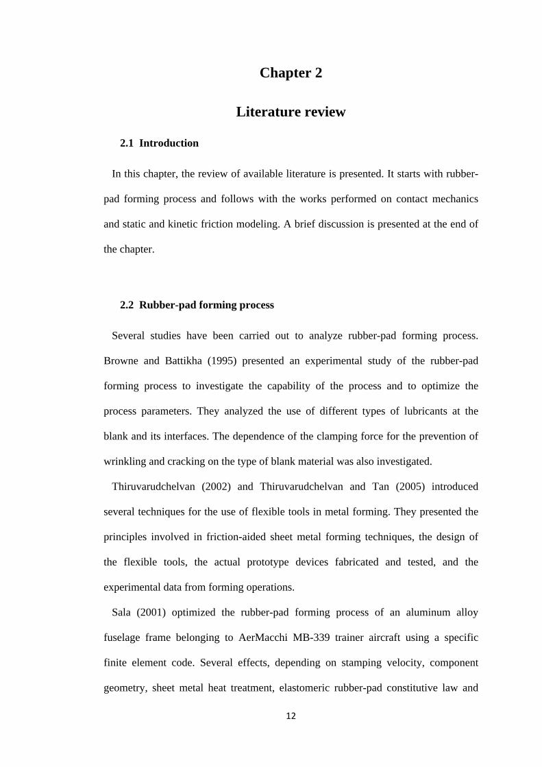
Several studies have been carried out to analyze rubber-pad forming process.
Browne and Battikha (1995) presented an experimental study of the rubber-pad
forming process to investigate the capability of the process and to optimize the
process parameters. They analyzed the use of different types of lubricants at the
blank and its interfaces. The dependence of the clamping force for the prevention of
wrinkling and cracking on the type of blank material was also investigated.
Thiruvarudchelvan (2002) and Thiruvarudchelvan and Tan (2005) introduced
several techniques for the use of flexible tools in metal forming. They presented the
principles involved in friction-aided sheet metal forming techniques, the design of
the flexible tools, the actual prototype devices fabricated and tested, and the
experimental data from forming operations.
Sala (2001) optimized the rubber-pad forming process of an aluminum alloy
fuselage frame belonging to AerMacchi MB-339 trainer aircraft using a specific
finite element code. Several effects, depending on stamping velocity, component
geometry, sheet metal heat treatment, elastomeric rubber-pad constitutive law and

13
thickness were taken into account. It was shown by his work that how the
preliminary tuning of these parameters lead to minimizing defects, increasing
component quality and reducing set-up times.
Dirikolu and Akdemir (2004) carried out a 3D finite element simulation study
concerning the flexible forming process to investigate the influence of rubber
hardness and blank material type on stress distribution in the formed blank. Their
investigations showed the effectiveness of finite element simulations in process
design and exposed the rubber hardness, blank material type, contact friction and die
design as crucial parameters that require adjustment before actual operations.
Peng et al. (2009) investigated the sheet soft punch stamping process to fabricate
micro channels via numerical simulations and experiments. Grain size of sheet metal,
hardness of soft punch and lubricant condition, were studied in details and the
numerical results were partially validated by experiments. They found that sheet
metal with small grain size is prone to obtain high formability. Larger friction
coefficient (up to 0.3) between the sheet and the rigid die may make the sheet
thinning quickly which decreases the formability, while the friction between the
sheet metal and the soft punch does not play an important role. They also reported
that the hardness of soft punch is not a decisive parameter to the final quality of the
workpiece.
2.3 Asperity contact models
When two solids are squeezed together they will in general not make atomic
contact everywhere within the apparent contact area and contact happens only on
peak asperities of surfaces. Tabor (1981) reviewed the state of understanding of
friction phenomenon as it existed three decades ago. Friction was originally thought

14
to be due to the resistance of asperities on one surface riding over the asperities of
the mating surface. The distinction between static and kinetic friction was attributed
to the asperities jumping over the gap between neighboring asperities on the other
surface during sliding.
Surface contact modeling is an essential part of any friction model (Adams et al.,
2003). It consists of two related steps. First, the equations representing the contact of
a single pair of asperities are determined. Second, the cumulative effects of
individual asperities are determined. Conventional multi-asperity contact models
may be categorized as predominately uncoupled or predominately coupled.
Uncoupled contact models represent surface roughness as a set of asperities, often
with statistically distributed parameters. The effect of each individual asperity is
local and considered separately from the other asperities; the cumulative effect is the
summation of the actions of individual asperities. Coupled models include the effect
of the loading on one asperity on the deformation of neighboring asperities. Such
models are far more complex mathematically than the uncoupled models and for that
reason have been used less frequently.
Hertz in 1882, presented the solution for the single asperity contact area between
two elastic bodies. The assumptions of Hertz contact problem are: (1) the contact
area is elliptical; (2) Each body is approximated by an elastic asperity loaded over an
elliptical contact area; (3) the dimensions of the contact area are small compared to
the dimensions of each body and to the radius of curvature of the surfaces; (4) the
strains are sufficiently small for linear elasticity to be valid; and (5) the contact is
frictionless and only a normal pressure is transmitted. In Hertz contact theory, area of
contact, contact radius and maximum contact pressure are given by simple equations
15
which depend upon the Young’s moduli, the Poisson’s ratios, the radius of curvature,
and the applied force (Carbone and Bottiglione, 2008).
In a pioneering study, Archard (1957) showed that in a more realistic model of
rough surfaces, where the roughness was described by a hierarchical model
consisting of small spherical bumps on top of larger spherical bumps and so on, the
area of real contact is proportional to the load. This model explains the basic physics
in a clear manner, but it cannot be used in practical calculations because real surfaces
cannot be represented by the idealized surface roughness assumed by Archard. A
somewhat more useful model, from the point of view of applications, was presented
by Greenwood and Williamson (1966). The Greenwood and Williamson model
assumes that in the contact between one rough and one smooth surface: (1) the rough
surface is isotropic; (2) asperities are spherical near their summits; (3) all asperity
summits have the same radius of curvature while their heights vary randomly with a
Gaussian distribution; (4) there is no interaction between neighboring asperities; and
(5) there is no bulk deformation. This model predicts that the area of real contact is
nearly proportional to the load. A more refined model based on the same picture was
developed by Bush et al. (1975). They approximated the asperities with paraboloids
to which they applied the Hertzian contact theory. The height distribution was
described by a random process, and they found that at low squeezing force the area
of real contact increases linearly with normal force. Several other contact theories are
reviewed in Carbone and Bottiglione (2008) and Persson (2006).
2.4 Static friction in rubber/metal contact
Static friction, defined as the tangential force required to initiate relative motion of
two contacting bodies, is associated with many important mechanical devices and
16
machines. A great amount of research work has been done in measuring and
modeling static friction. The elastic-plastic spherical contact under combined normal
and tangential loading is a classical problem in contact mechanics which is
applicable in modeling of friction between rough surfaces. The treatment of
combined normal and tangential loading of elastic spherical contact stems from the
classical work of Mindlin (1949). According to the Mindlin model, the contact area
between two spheres under combined loading consists of a central stick region
surrounded by an annular slip zone. As the tangential load increases, the central stick
region gradually diminishes and finally disappears. At this moment full sliding
begins which satisfies the Coulomb friction law, that is, the tangential load equals the
product of the normal load and a predefined static friction coefficient. The normal
loading in this work is assumed frictionless, and the contact area and pressure
distribution follow the Hertz solution even when the tangential load is applied.
Chang, Etsion and Bogy (1988) presented a model (CEB friction model) for
predicting the static friction coefficient of rough metallic surfaces. The CEB friction
model uses a statistical representation of surface roughness following a Gaussian
distribution and calculates the static friction force that is required to fail all of the
contacting asperities, taking into account their normal preloading. In CEB model, the
mechanism involves plastic flow of pre-stressed asperities. Related to the
temperature, possible static friction mechanisms are the asperity creep at lower
temperatures and welding of asperities at higher temperatures.
Rubber/metal contact is found in a large variety of applications, such as rubber-pad
forming processes, vibration control applications, power transmission systems and
seals. There are many papers in the literature about rubber friction regarding kinetic
friction (see, e.g., Persson et al., 2003), but only a few concerning static friction. The

17
static friction force was investigated by Roberts and Thomas (1976) for smooth
rubber hemispheres in contact with glass plates. Their experiments carried out on soft
rubber suggest that the magnitude of the static friction force is related to the elastic
deformation of rubber prior to the appearance of the elastic instabilities.
The preliminary stage of friction was studied experimentally by Barquins (1993) in
rubber/glass contact. The evolution of the contact area was recorded by means of a
camera mounted on an optical microscope. Superimposing the frames has shown a
contact area which comprises a central adhesive zone, surrounded by an annulus of
slip. Friction forces were measured with the help of an elastic system and
displacement transducers.
The experiments of Adachi et al. (2004) carried out on rubber balls in contact with
glass plates revealed also the process of partial slip and its propagation with
increasing tangential load as described theoretically by Mindlin (1949).
Deladi et al. (2007) developed a static friction model for rubber/metal contact that
takes into account the viscoelastic behaviour of rubber. This model is based on the
contact of a viscoelastic/rigid asperity couple. Single asperity contact was modeled in
such a way that the asperities stick together in a central region and slip over an
annulus at the edge of the contact. The slip area increases with increasing tangential
load. Consequently, the static friction force is the force when the slip area is equal to
the contact area. Using the model, the traction distributions, contact area, tangential
and normal displacement of two contacting asperities were calculated. The single
asperity model was then extended to multi-asperity contact, suitable for rough
surfaces.

18
2.5 Kinetic friction in metal/metal contact
From the early experimental work of Amontons in 1699, it was observed that
friction is directly proportional to the applied load and independent of the surface
nominal contact area. Coulomb in 1785, completed Amontons work with the third
law that kinetic friction force is independent of sliding velocity. These early
observations gave rise to the classic laws of friction, which resulted in a
proportionality constant, known as the friction coefficient. However, today it is well
recognized that friction coefficient values depend on many other conditions besides
the contacting material pairs, such as surface roughness, lubricant viscosity, surface
energy, contact load and temperature.
The development of kinetic friction models for SMF simulations is complicated by
the fact that any of a variety of lubrication regimes may co-exist in the sheet/tooling
interface. Wilson (1979) described four basic lubrication regimes in metal working:
thick film, thin film, mixed and boundary lubrication regimes. Moreover, he showed
that the traditional Coulomb friction model is inappropriate for sheet metal forming
simulations, because it does not predict the lubrication regimes. Schey (1983)
provided a review of many different ways of measuring or inferring friction in metal
forming operations. One of the most useful methods is that of Schey (1996) who
explored the effect of drawing speed and lubricant viscosity on coefficient of friction
using drawbead simulation tests. The results showed that the coefficient of friction
decreases with increasing the viscosity × velocity product. Saha et al. (1996)
investigated the relationship between friction and process variables including sliding
speed, strip strain and strain rate in the boundary lubrication regime using a sheet
metal forming simulator which stretches a strip around a cylindrical pin. Friction was
found to decrease with increasing sliding velocity for all test conditions.
19
Stribeck (1902) is credited for carrying out the first systematic experiments
unfolding a clear view of the characteristic curve of the coefficient of kinetic friction
versus speed. In recognition of his contribution, this curve is called the “Stribeck
curve” (Jacobson, 2003). Works on the Stribeck curve fall into two categories: one is
the experimental examination of its variation by altering the material property, the
surface finish, the viscosity of the oil, and the operating conditions; the other is
theoretical exploration of its behavior that parallels the development of the modeling
of mixed lubrication.
In Gelinck and Schipper (2000), a model is presented in order to predict the
Stribeck curves for line contacts. This model is based on the combination of the
Greenwood and Williamson (1966) contact model and the full film theory using the
mixed lubrication model of Johnson et al. (1972). With this model, one is able to
predict friction and determine the transitions between the different lubrication
regimes: elasto-hydrodynamic lubrication (EHL), mixed lubrication (ML), and
boundary lubrication (BL) regimes. This model is based on the assumption that
enough lubricant is supplied to the contact, e.g., fully flooded conditions.
Faraon and Schipper (2007) developed a mixed lubrication model in order to
predict the Stribeck curves for starved lubricated line contact. This model is based on
a combination of the contact model of Greenwood and Williamson (1966) and the
elasto-hydrodynamic (EHL) film thickness for starved line contacts.
In the work of Wolveridge et al. (1971), a correction on the film thickness formula
for line contacts due to starvation is presented. Combining this modified film
thickness relation for starved line contacts with the model of Gelinck and Schipper
(2000) will result in a mixed lubrication model for starved lubricated line contacts.

20
Lu et al. (2006) presented the Stribeck curves of a series of experiments under
various oil inlet temperatures and loads and verified the curves with a theoretical
model. This model is based on the Bair and Winer model (1979) to describe the shear
stress of the lubricant. Their theoretical analysis provided a simple, but realistic
model, for prediction of Stribeck curves.
2.6 Conclusion
The various literature reviewed in this chapter has shown that to date, the models
of friction which take into account the various local contact conditions such as
velocity, pressure, lubricant viscosity, roughness and temperature are available and
have been well researched. The published work to date only used Coulomb friction
model in the rubber-pad forming simulations. The application of such static and
kinetic friction models on rubber-pad forming simulations have not been reported
anywhere. The existence of various lubrication regimes in metal working would
suggest that Coulomb friction model is inadequate for application in SMF
simulations. It necessitates the application of new friction models in SMF
simulations to ensure the accuracy and efficiency of finite element simulations and
therefore the static and kinetic friction models suitable for rubber-pad forming
process are studied in this thesis.

21
Chapter 3
Static and kinetic friction models for rubber-pad forming
3.1 Introduction
When a metal forming process is observed, it is clear that the conditions in all the
different contacts are very different. For most forming simulations the value of
coefficient of friction is taken as a constant, neglecting the fact that friction depends
on a large number of parameters, e.g., the micro-geometry, the macro-geometry, the
lubricant and the operational parameters: velocity, temperature and normal load. If
one of the parameters changes, the coefficient of friction will also change (Matuszak,
2000). Often, several metal forming simulations with different values for the
coefficient of friction have to be performed before the simulation provides acceptable
results. It is clear that these simulations have no predicting power at all (Lee et al.,
2002) and friction models based on local contact conditions are needed.
In this chapter, at first a single-asperity static friction model is presented and
subsequently, a multi-asperity static friction model between viscoelastic asperities
and a rigid flat under combined normal and tangential loading condition is developed
for rubber-pad/metal sheet contact taking into account the viscoelastic behaviour of
rubber and local contact conditions. Subsequently, a kinetic friction model is
developed for die/metal sheet contact based on Stribeck frictional behavior.
3.2 Coulomb friction model
The easiest and probably the most well known friction model is Coulomb friction
model. Though it greatly over simplifies the frictional phenomena it is widely used to

22
describe the friction in mechanical contacts. In this model, the ratio between friction
force and normal force, defined as the coefficient of friction, is considered to be
constant. Coulomb friction model can be formulated as
ncf FF μ= (3.1)
where cμ is the Coulomb coefficient of friction, fF is the sliding friction force and
nF the normal load in the contact.
3.3 Single-asperity static friction model for rubber/metal contact
The contact between surfaces is composed of many asperity couples that carry the
load. The first step in modeling two surfaces in contact is based on the determination
of the contact parameters between a pair of asperities (Deladi et al., 2007). When two
elastic spherical asperities are loaded by a normal force nF , the radius of the contact
circle, the pressure and the normal approach are given by Hertz theory. If,
subsequently, a tangential force tF is applied, the shear stress within the contact and
the tangential displacement of bodies are specified by Mindlin theory. According to
Mindlin (1949), the resulting infinite tangential traction at the edge of the contact is
released by micro-slip and the contact area comprises a stick region surrounded by an
annulus of slip (see, Figure 3.1). This micro-slip can be calculated using the solution
proposed by Johnson (1985).

23
Figure 3.1 Evolution of the contact area (top view) according to Mindlin theory (Mindlin, 1949).
Rubber materials exhibit both elasticity and viscous resistance to deformation. The
materials can retain the recoverable (elastic) strain energy partially, but they also
dissipate energy if the deformation is maintained. Viscoelasticity is the property of
materials that exhibit both viscous and elastic characteristics when undergoing
deformation. Viscous materials resist shear flow and strain linearly with time when a
stress is applied. Elastic materials strain instantaneously when stretched and just as
quickly return to their original state once the stress is removed. Viscoelastic materials
behaviour can be modeled using springs and dashpots connected in series and/or in
parallel. A dashpot is connected in parallel with a spring in Figure 3.2(a). This is
known as a Voigt element. If deformed, the force in the spring is assumed to be
proportional to the elongation of the assembly, and the force in the dashpot is
assumed to be proportional to the rate of elongation of the assembly. With no force
acting upon it, the assembly will return to its reference state that is dictated by the

24
rest length of the spring. In this model, if a sudden tensile force is applied, some of
the work performed in the assembly is dissipated in the dashpot while the remainder
is stored in the spring. The applied force is analogous to the deforming stress and the
elongation is analogous to the resulting strain. The viscous resistance to deformation
represented by the dashpot introduces time dependency to the response of the
assembly where this dependency is dictated by the spring and dashpot constants.
A dashpot is connected in series with a spring is shown in Figure 3.2(b). This is
called a Maxwell element. In this assembly, if a sudden tensile force is applied, it is
the same in both the spring and the dashpot. The total displacement experienced by
the element is the sum of the displacements of the spring and the dashpot. The
response of rubber to changes in stress or strain is actually a combination of elements
of both mechanical models (see, Figure 3.2(c)). The response is always time-
dependent and involves both the elastic storage of energy and viscous loss.
Figure 3.2 Mechanical models representing the response of viscoelastic materials: (a) Voigt model, (b) Maxwell model, (c) SLS model.
The Standard Linear Solid (SLS) model gives a relatively good description of both
stress relaxation and creep behavior. Stress relaxation is the time-dependent decrease